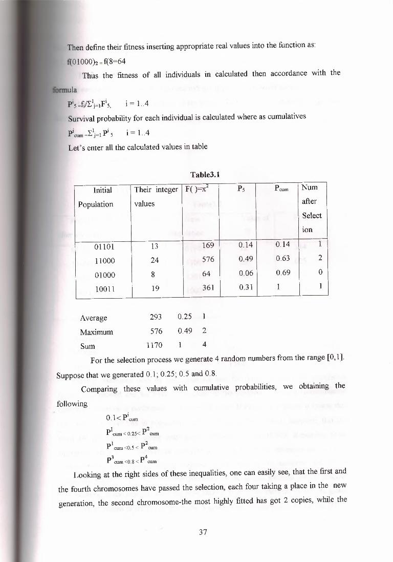
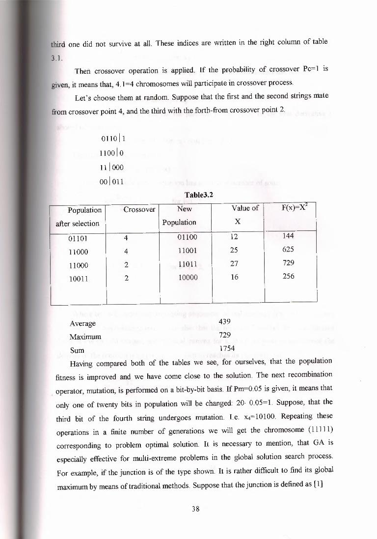
NEAR EAST UNIVERSITY Faculty of Engineering Department of Computer Engineering Genetic Algorithm Based Optimization Graduation Project COM-400 Student: Yahya Safarinı I ~Supervisor: Assoc. Prof. Dr. Rahib Abiyev Nicosia - 2003
Transcript
NEAR EAST UNIVERSITY
Faculty of Engineering
Department of Computer Engineering
Genetic Algorithm Based Optimization
Graduation ProjectCOM-400
Student: Yahya Safarinı
I
~Supervisor: Assoc. Prof. Dr. Rahib Abiyev
Nicosia - 2003
ACKNOWLEDGEMENTS
"First I would like to thank my supervisor Assoc. Prof Dr. Rahib Abiyevfor his great
advice andrecommendations tofinish this workproperly.
Although Ifaced manyproblem collections data but has guiding me the appropriate
references.(DR Rahib) thanks a lotfor your invaluable and continual support.
Second, I would like to thank myfamilyfor their constant encouragement and support
during thepreparation of this work specially my brothers (Mohammed and Ahmed) .
Third, I thank all the staff of thef acuity of engineeringfor giving me thefacilities to
practice and solving any problem I was.facing during working in thisproject.
Forth I do not want toforget my bestfriends (Mana.I),(Saleh),(Abu habib) and all
friendsfor helping me tofinish this work in short time by their invaluable
encouragement.
Finally thanksfor all of myfriends for their advices and support specially Terak
Ahmed,Mohammed Darabie ,Anas Badran,Adham Sheweiki ,Bilal Qarqour and
Mohammad Qunj.
ABSTRACT
By increasing complexity of processes, it has become very difficult to control them on the base of
traditional methods. In such condition it is necessary to use modem methods for solving these
problems. One of such method is global optimization algorithm based on mechanics of natural
selection and natural genetics, which is called Genetic Algorithms. In this project the application
problems of genetic algorithms for optimization problems, its specific characters and structures
are given. The basic genetic operation: Selections, reproduction, crossover and mutation
operations are widely described the affectivity of genetic algorithms for optimization problem
solving is shown. After the representation of optimizations problem, structural optimization and
the finding of optimal solution of quadratic equation are given.
The practical application for selection, reproduction, crossover, and mutation operation are
shown. The fiınctional implementation of GA based optimization in MATLAB programming
language is considered. Also the multi-modal optimization problem, some methods for global
optimization and the application of Niching method for multi-modal optimization are discussed.
11
TABLE OF CONTENTS
ACKNOWLEDGEMENTSABSTRACTTABLE OF CONTENTSINTRODUCTIONCHAPTER ONE: WHAT ARE GENETIC ALGORITHMS (GAs)?
l. 1 What are Genetic Algorithms (GAs)?1.2 Defining Genetic Algorithms1.3 Genetic Algorithms: A Natural Perspective1. 4 TheIteration Loop of a Basic Genetic Algorithm1.5 Biology1.6 An Initial Population of Random Bit Strings is Generated1. 7 Genetic Algorithm Overview
1. 7.1 A Number of Parameters Control The Precise Operation of The GeneticAlgorithm, viz.
2.7 Multi-Objective Optimization for Highway Management ProgrammingCHAPTER THREE: A GENETIC ALGORITHM-BASED
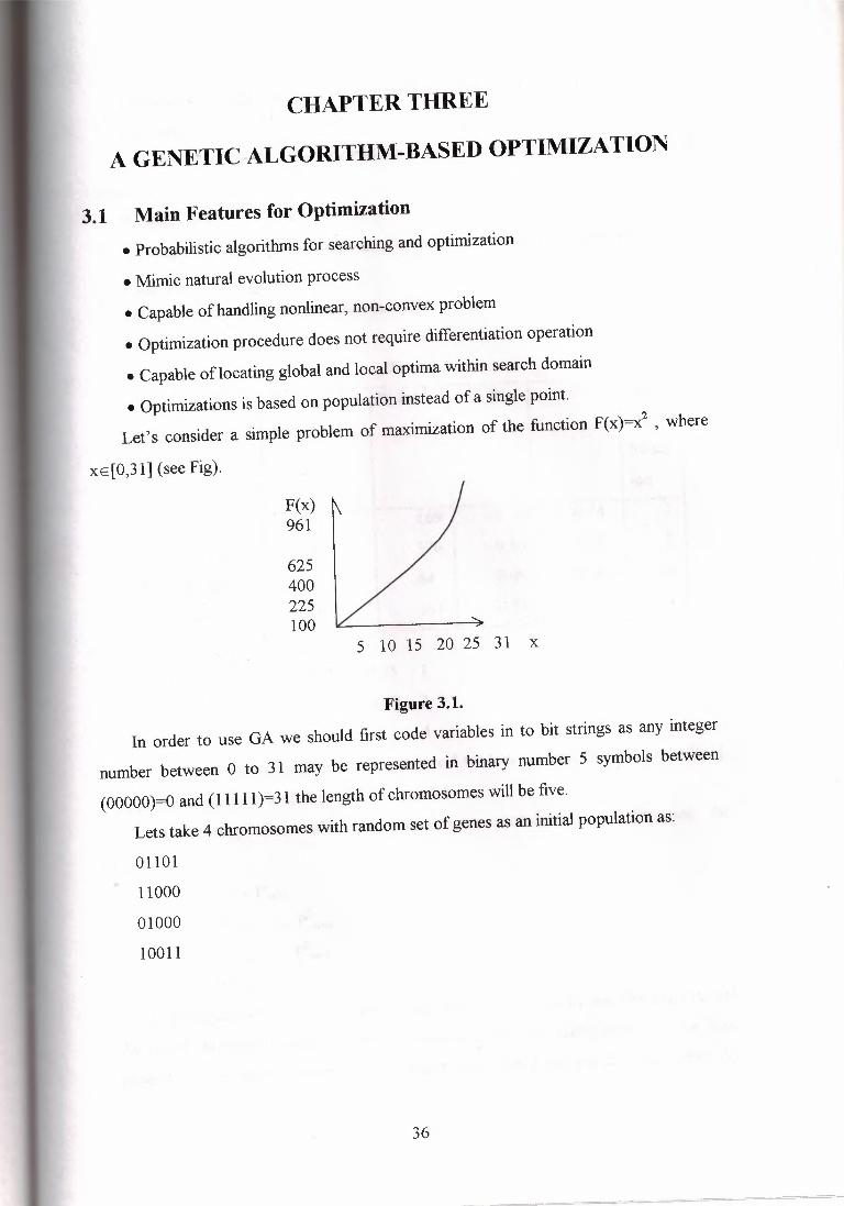
OPTIMIZATION3 .1 Main Features for Optimization
3. 1. 1 Representation3.2 Applications
3 .2.1 Difficulties3.2.2 Deception
3 .3 The Neighborhood Constraint Method:A Genetic Algorithm-BasedMultiobjeetive Optimization Technique3.3. l. Overview3.3.2 Literature Review: GAs in Mo Analysis
iii
.I..
il...Ill
133345556
79
101011
121414141618182429 2930303132
36 3640 434445
464648
INTRODUCTION
This is an introduction to genetic algorithm methods for optimization. Genetic
Algorithms were formally introduced in the United States in the 1970s by John Holland
at University of Michigan. The continuing price/performance improvements of
computational systems has made them attractive for some types of optimization. In
Particular, genetic algorithms work very well on mixed (continuous and discrete),
Combinatorial problems. They are less susceptible to getting 'stuck' at local optima than
gradient search methods. But they tend to be computationally expensive.
To use a genetic algorithm, you must represent a solution to your problem as a
genome (or chromosome). The genetic algorithm then creates a population of solutions
and applies genetic operators such as mutation and crossover to evolve the solutions in
order to find the best one(s).This presentation outlines some of the basics of genetic algorithms. The three most
important aspects of using genetic algorithms are: (1) definition of the objective
function, (2) definition and implementation of the genetic representation, and (3)
definition and implementation of the genetic operators. Once these three have been
defined, the generic genetic algorithm should work fairly well. Beyond that you can try
many different variations to improve performance, find multiple optima (species - if
they exist), or parallelizethe algorithms.The genetic algorithm uses stochastic processes, but the result is distinctly non
random (better than random).GENETIC Algorithms are used for a number of different application areas. An
example of this would be multidimensional OPTIMIZATION problems in which the
character string of the CHROMOSOME can be used to encode the values for the
different parameters being optimized.In practice, therefore, we can implement this genetic model of computation by
having arrays of bits or characters to represent the Chromosomes. Simple bit
manipulation operations allow the implementation of CROSSOVER, MUTATION and
other operations. Although a substantial amount of research has been performed on
variable- length strings and other structures, the majority of work with GENETIC
Algorithms is focused on fixed-length character strings. We should focus on both this
aspect of fixed-length ness and the need to encode the representation of the solution
1
being sought as a character string, since these are crucial aspects that distinguish
GENETIC PROGRAMMING, which does not have a fixed length representation and
there is typically no encoding of the problem.
When the GENETIC ALGORITHM is implemented it is usually done in a manner
that involves the following cycle: Evaluate the FITNESS of all of the Individuals in the
POPULATION. Create a new population by performing operations such as
CROSSOVER, fitness-proportionate REPRODUCTION and MUTATION on the
individuals whose fitness has just been measured. Discard the old population and iterate
using the new population.
One iteration of this loop is referred to as a GENERATION. There is no
theoretical reason for this as an implementation model. Indeed, we do not see this
punctuated behavior in Populations in nature as a whole, but it is a convenient
implementation model.
The first GENERATION (generation O) of this process operates on a
POPULATION of randomly generated Individuals. From there on, the genetic
operations, in concert with the FITNESS measure, operate to improve the population.
2
CHAPTER ONE
WHAT ARE GENETIC ALGORITHMS (GAs)?
1.1 What Are Genetic Algorithms (GAs)?
Genetic Algorithms (GAs) are adaptive heuristic search algorithm based on
the evolutionary ideas of natural selection and genetics. As such they represent an
intelligent exploitation of a random search used to solve optimization problems.
Although randomised, GAs are by no means random, instead they exploit historical
information to direct the search into the region of better performance within the search
space. The basic techniques of the GAs are designed to simulate processes in natural
systems necessary for evolution, specially those follow the principles first laid down by
Charles Darwin of "survival of the fittest.". Since in nature, competition among
individuals for scanty resources results in the fittest individuals dominating over the
weaker ones.
1.2 Defining Genetic Algorithms
What exactly do we mean by the term Genetic Algorithms Goldberg (1989) defines
it as:
Genetic algorithms are search algorithms based on the mechanics of natural
selection and natural genetics.
Bauer (1993) gives a similar definition in his book:
Genetic algorithms are software, procedures modeled after genetics and evolution.
GAs exploits the idea of the survival of the fittest and an interbreeding population
to create a novel and innovative search strategy. A population of strings, representing
solutions to a specified problem, is maintained by the GA. The GA then iteratively
creates new populations from the old by ranking the strings and interbreeding the fittest
to create new strings, which are (hopefully) closer to the optimum solution to the
problem at hand. So in each generation, the GA creates a set of strings from the bits and
pieces of the previous strings, occasionally adding random new data to keep the
population from stagnating. The end result is a search strategy that is tailored for vast,
complex, multimodal search spaces. GAs are a form of randomized search, in that the
way in which strings are choisen and combined is a stochastic process. This is a
radically different approach to the problem solving methods used by more traditional
3
;a:1g-0ridm:ıs, whlclh tend to /be mor-e rdeterministirc in nature, :sur.ch as tlre :gm<lfient methods
used to find ııınifilinm iırn gra,pıh. theory."l"'iı., :·,;ıı., of .·· ·'·'ı,-.x-.;riL, il!:ı,.,,....'.·, ,_,j' .. ··,11-:· ... ··•.····· ·•· .....•. ,-, .. 1,.... ,,·,ı.._. G·.. ;A,-!L,uı.e ıaea o, sııfVi!Va or me :u1ı.te.,,L ts oı g,ı:rea:1. ım:portance to .geootrc aıgor,ıtmus. , -~
use wıhat is ter.med as a fitness fü;fl.'ction in order to :s-e'rett tlre fütest string that wiU he"'"'""';;ı .•....,, '"'f-~"'4'C '"'""'"""" '"..,,,;.ı "''"'""·O· ..;;,,c.,ıı,.·~·u better '1'1""''fi"1'"'h""'""' n.'f. ,.,..,...,.,,..l('TI;!_ T·!ı...,. 4!.t· ness -~···.....-,...t· '"""'·u.:,.v.Uıı.-v~, ·\ı..laıl.1- · )liıv:v,v., ~ıdi ·vv:ı'.r·,\;11.··v'a!IJJ:~j , ·."'' :L',;.,'1~ )l-"V,t'-u.i,a.:t(ı,\..!M.:ıııı ·,Jv ;~:vıtılUJJ!iı.:r... ' il.1""1 il· :111~3 ..,t!U,;1,1\.:i· lıuaıı
takes 'a ,,.,+,.;;..,,,o """",ıı '"''S'.S''"'"""·S .,. 11',,;t,.,,:+;;~,,,,. fitness "~-~'""' to ...;t,..e· 'S;ı...:;...,,_o-'. '7':'l,.e·· ,.,.,.;1,.,,.,.,;ı bv n,,t.:;,C. 'IL ;,.ilf.cv.t\j\,;,. ,. ,.:Ml.tL'.lı~t:, :wu,U ı.u ·~J;,;,ıı,\ı,. s:a .iJ.1\ı;:,\l·af\:.ıN1.\a:, 111:UJ. , .. , 'v0W·uv 1ı: liff,, 't.1.;1/1.i.J,::,·· lllll. · llıI\ı:ı't..:llvU U_-.:7 ·.vv!llf,:ı... aa -1ıiL-
does this and tllre tı.:ature of the füness vahıe does n:ot matter.. The o-ftly tm~gthat thefitness function m.:ust do is to rank the strl@gs in some w~y by -pırodurdng the fitnessv:allue.. These values are thm used to select the fitte-st :strings. The connept of a fi'.me,ss.il::--,,-+:· ' ,... :' ~ . t . . .,,.;.'.· .. 1.~' '.•.... t' - ' • ··r' - ' " •' . " .... --,1 ..ıı.;r - ,· " .... ' ·' :t..,. ' l.,>, ' ; .• .;ı;mı\,;\,,ı:on ıs, m rao ., a pa<,d'CU.'ıar ımsc ance o- ;a more :gerreıw. ,h;ı "'o:ncept, tı,e ouJectıve
fu.m.tion.
1.3 Genetic Algorithms: A Natural PerspectiveThe popula:tron can be 'siın;p:iy viewed as a ooUreotion ,of il1I-terarct'i~g creatures. As
each ,geı:rerationcf creatures eomes :antl goes, tke weaker ones ttre:rı'd to dire away without
pr-0:durci~g ,dlnl-d:ren~ wmle the stronger mate, 'C'omlrimng :attributıes of both pasrrems, toproduce ft'ew, :a;nd p:erha;ps unique children to ron'.tinue t1tre cycle. Oooa:srorrally~ a'"''"U"''"' .•. ~""""" IA'f'°'JelO(rı,·s ;,.,..,,,. 'O'"'"" ,,..,r· the creanrres d' :ı·.•,..,..•.•..;,;~,,_,,.,o ·11-'il-,z. fi·o· ··p· .,.,.....,-;.,,.... ""'"'"""' "'"''O' ,,,,,.-:u:ı: · .!ı..ıwu,v.1.<.1. vı,, '-'F .ı.ıiı.<J.il,O r :.u.v 'V1 ıvıı · \ ..:ı:ı:\,,;,O. · , -: ; ·v..""'ı~a.j'\ı:ı~.e,:vu-".\., t'· .·; ;:..wıcu.ıu.;1a.ı. '\,,:ı'\""1:;:J.iı. qıı.,1. ·:i.l.".'.\.:.ı-.
Rreme:mber thaıt in nature, a diverse population within a species ite.tıd:s to al'low the
species to :ad:a;pt to i:t':s en.vironm.ınt with more ease. The same holds true for genetic:aJJ.gori'thms,.
4
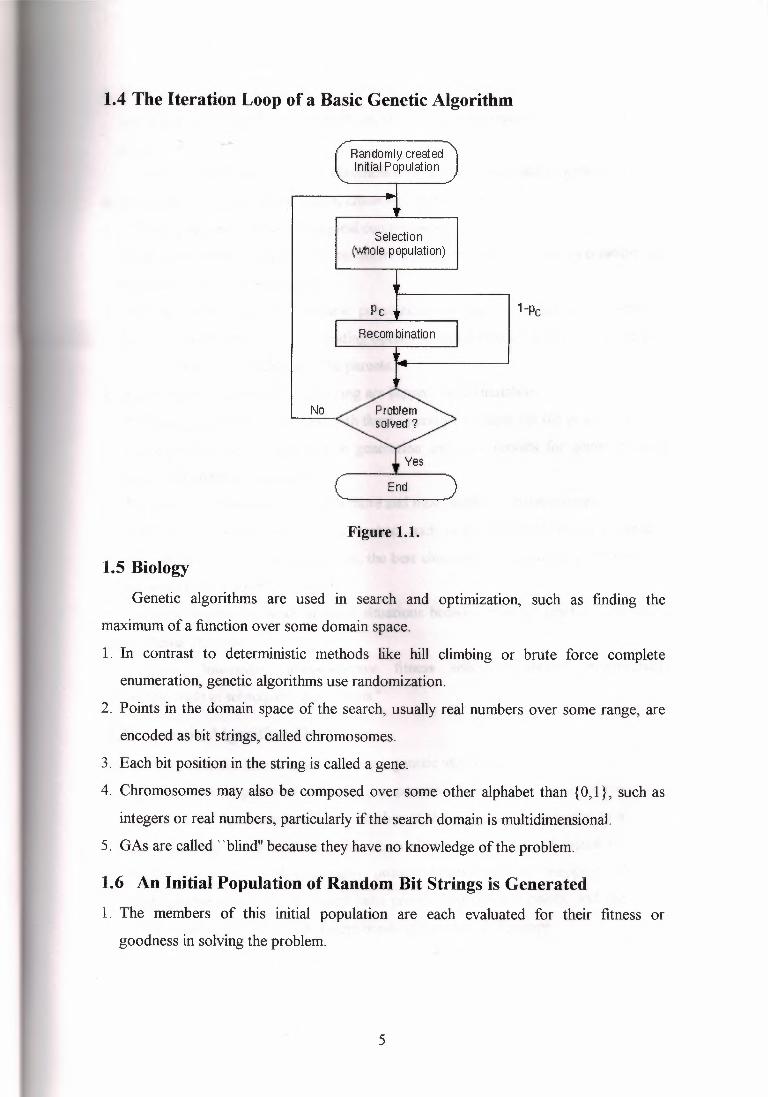
1.4 The Iteration Loop of a Basic Genetic Algorithm
Rarıdomlycreatedlnltial Population
Selection(v.ıtıoıe population)
Pc 1-Pc
Recom bination
No
End
Figure 1.1.
1.5 BiologyGenetic algorithms are used in search and optimization, such as finding the
maximumof a function over some domain space.
1. In contrast to deterministic methods like hill climbing or brute force complete
enumeration, genetic algorithmsuse randomization.
2. Points in the domain space of the search, usually real numbers over some range, are
encoded as bit strings, called chromosomes.
3. Each bit position in the string is called a gene.
4. Chromosomes may also be composed over some other alphabet than {0,1}, such as
integers or real numbers, particularly if the search domain is multidimensional.
5. GAs are called "blind" because they have no knowledge of the problem.
1.6 An Initial Population of Random Bit Strings is Generated1. The members of this initial population are each evaluated for their fitness or
goodness in solving the problem.
5
2. If the problem is to maximize a function f(x) over some range [a,b] of real numbers
and if f(x) is nonnegative over the range, then f(x) can be used as the fitness of the bit
string encoding the value x.
From the initial population of chromosomes, a new population is generated using
three genetic operators: reproduction, crossover, and mutation.
1. These are modeled on their biological counterparts.
2. With probabilities proportional to their fitness, members of the population are
selected for the new population.3. Pairs of chromosomes in the new population are chosen at random to exchange
genetic material, their bits, in a mating operation called crossover. This produces two
new chromosomes that replace the parents.
4. Randomly chosen bits in the offspringare flipped, called mutation.
The new population generated with these operators replaces the old population.
1. The algorithm has performed one generation and then repeats for some specified
number of additional generations.2. The population evolves, containingmore and more highlyfit chromosomes.
3. When the convergence criterion is reached, such as no significant further increase in
the average fitness of the population, the best chromosome produced is decoded into
the search space point it represents.Genetic algorithms work in many situations because of some hand waving called
The Schema Theorem.'' Short, low-order, above-average fitness schemata receive exponentially
increasing trials in subsequent generations."
1.7 Genetic Algorithm OverviewGOLD optimises the fitness score by using a genetic algorithm.
1. A population of potential solutions (i.e. possible docked orientations of the
ligand) is set up at random. Each member of the population is encoded as a
chromosome, which contains information about the mapping of ligand H
bond atoms on (complementary) protein H-bond atoms, mapping of
hydrophobic points on the ligand onto protein hydrophobic points, and the
conformation around flexibleligand bonds and protein OH groups.
6
2. Each chromosome is assigned a fitness score based on its predicted binding
affinity and the chromosomes within the population are ranked according to
fitness.
3. The population of chromosomes is iteratively optimised. At each step, a
point mutation may occur in a chromosome, or two chromosomes may mate
to give a child. The selection of parent chromosomes is biased towards fitter
members of the population, i.e. chromosomes corresponding to ligand
<lockings with good fitness scores.
1.7.1 A Number of Parameters Control The Precise Operation of TheGenetic Algorithm, viz.
1. Population size.
2. Selection pressure.
3. Number of operations.
4. Number of islands.
5. Niche size.
6. Operator weights: migrate, mutate, crossover.
7. Annealingparameters: van der Waals, hydrogen bonding.
1.7.1.1 Population Size
1. The genetic algorithm maintains a set of possible solutions to the problem. Each
possible 'solution is known as a chromosome and the set of solutions is termed apopulation.
2. The variable Population Size (or popsize) is the number of chromosomes in
the population. If n_islands is greater than one (i.e. the genetic algorithm is
split over two or more islands), pop size is the population on each island.
1.7.1.2 Selection Pressure
1. Each of the genetic operations (crossover, migration, mutation) takes
information from parent chromosomes and assembles this information in
child chromosomes. The child chromosomes then replace the worst
members of the population.
2. The selection of parent chromosomes is biased towards those of high fitness,
i.e. a fit chromosome is more likelyto be a parent than an unfit one.
. 3. The selection pressure is defined as the ratio between the probability that the
most fit member of the population is selected as a parent to the probability
7
that an average member is selected as a parent. Too high a selection pressure
will result in the population converging too early.
4. For the GOLD docking algorithm, a selection pressure of 1. 1 seems
appropriate, although 1. 125 may be better for library screening since the aim
is for faster oonvergeeoe
1.7.1.3 Number of Operations
1. The genetic algorithm starts off with a random population (each value in
every chromosome is set to a random number). Genetic operations
(crossover, migration, mutation are then applied iteratively to the population.
The parameter Number of Operations (or maxops) is the number of
operators that are applied over the course of a GA run.
2. It is the key parameter in determininghow long a GOLD run will take.
1.7.1.4 Number of Islands
1 . Rather than maintaining a single population, the genetic algorithm can
maintain a number of populations that are arranged as a ring of islands.
Specifically, the algorithm maintains n_islands populations, each of size
popsıze.
2. Individuals can migrate between adjacent islands using the migration
operator.
3. The effect of n_islands on the efficiencyof the genetic algorithm is uncertain.
1.7.1.5 Niche Size
1 . Niching is a common technique used in genetic algorithms to preserve diversity
within the population.
2. In GOLD, two individuals share the same niche if the rmsd between the coordinates
of their donor and acceptor atoms is less than 1. O A.3. When adding a new individual to the population, a count is made of the number of
individuals in the population that inhabit the same niche as the new chromosome. If
there are more than NicheSize individuals in the niche, then the new individual
replaces the worst member of the niche rather than the worst member of the total
1. The operator weights are the parameters Mutate, Migrate and Crossover (or
Pt_cross).2. They govern the relative frequencies of the three types of operations that can
occur during a genetic optimization: point mutation of the chromosome,
migration of a population member from one island to another, and crossover
(sexual mating) of two chromosomes.3. Each time the genetic algorithm selects an operator, it does so at random. Any
bias in this choice is determined by the operator weights. For example, if
Mutate is 40 and Crossover is 1 O then, on average, four mutations will be
applied for every crossover.4. The migrate weight should be zero if there is only one island, otherwise
migration should occur about 5% of the time.
1.7.1.7 Annealing Parameters: van der Waals, hydrogen bonding
1. The annealing parameters, van der Waals and Hydrogen Bonding, allow poor
hydrogen bonds to occur at the beginning of a genetic algorithm run, in the
expectation that they will evolve to better solutions.2. At the start of a GOLD run, external van der Waals (vdw) energies are cut off
when Eij > van der Waals * kij, where kij is the depth of the vdw well
between atoms i and j. At the end of the run, the cut-off value is FINISH
VDW LINEAR CUTOFF.3. This allows a few bad bumps to be tolerated at the beginning of the run.
4. Similatlythe parameters Hydrogen Bonding andFINAL_VIRTUAL_PT~MATCH_MAX are used to set starting and finishing
values ofmax distance (the distance between donor hydrogen and fitting
point must be less than max_distance for the bond to count towards the
fitness score). This allows poor hydrogen bonds to occur at the beginning of a
GA run.5. Both the vdw and H-bond annealing must be gradual and the population
allowed plenty oftime to adapt to changes in the fitness function.
1.8 Genetic OperationsIn order to improve the current population, genetic algorithms commonly use three
different genetic operations. These are reproduction, crossover, and mutation. Both
9
reproduction and crossover can be viewed as operations that force the population to
converge. They do this by promoting genetic qualities that are already present in the
population. Conversely, mutation promotes diversity within the population. In general,
reproduction is a fitness preserving operation, crossover attempts to use current positive
attributes to enhance fitness, and mutation introduces new qualities in an attempt to
increase fitness.
1.8.1 Reproduction
The reproduction genetic operation is an asexual operation. Reproduction involves
making an exact copy of an individual from the current population into the next
generation. The selection of which individuals will be copied into the next generation is
done probabilistically based upon relative fitness. Suppose that a gene g exists such
that \Ih F (g) ~ F (h) . Then the reproduction operation will be performed on gene h
with a probability;~;~ . This selection method ensures all valid genes (i.e. genes that
actually solve the problem) have a probability of being chosen for the reproduction
operation since F(h) > O for all genes h that represent a valid solution to the problem
that is being solved.
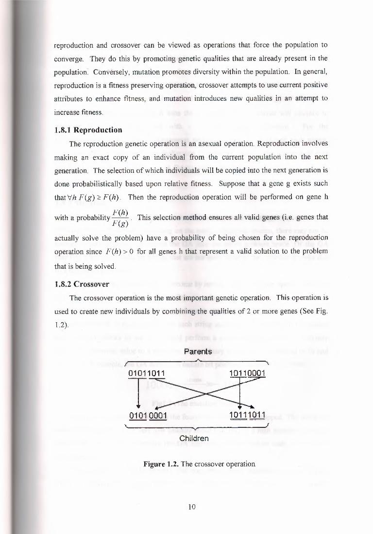
1.8.2 Crossover
The crossover operation is the most important genetic op,eration. This operation is
used to create new individuals by combining the qualities of 2 or more genes (See Fig.
1.2).
Parents
01011011
T10110001
0101 0001--- 10111011~~
Children
Figure 1.2. The crossover operation
10
A decision must be made as to which individuals are to be involved in the
crossover operation. The method that was used to make this decision in the genetic
algorithms under consideration is a form of Boltzmann tournament selection. A
Boltzmann tournament proceeds as follows: two genes g and h are selected at random
from the current population and are entered into a tournament. If F(g) > F(h) then g
wins the tournament, otherwise h wins the tournament. The winner will advance to
compete in another tournament with a randomly chosen individual. For the
implementation, there were 3 tournaments performed in order to choose each parent.
The most general statement of a Boltzmann tournament requires the selection of h to
satisfyIF (g) - F(h)! 2 <f; , for some ¢> [Mafoud9l]. For the implementations, a value of
</> = O was used.
1.8.3 Mutation
Selection and crossover alone can obviously generate a staggering amount of
differing strings. However, depending on the initial population chosen, there may not be
enough variety of strings to ensure the GA sees the entire problem space. Or the GA
may find itself converging on strings that are not quite close to the optimum it seeks due
to a bad initialpopulation.
Some of these problems are overcome by introducing a mutation operator into the
GA. The GA has a mutation probability, m, which dictates the frequency at which
mutation occurs. Mutation can be performed either during selection or crossover
(though crossover is more usual). For each string element in each string in the mating
pool, the GA checks to see if it should perform a mutation. If it should, it randomly
changes the element value to a new one. In our binary strings, 1 s are changed to Os and
Os to 1 s. For example, the GA decides to mutate bit position 4 in the string 10000:
10000 Mutate :ıııı 10010
Figl.3 .The mutation operator
The resulting string is 1001 O as the fourth bit in the string is flipped. The mutation
probability should be kept very low (usually about 0.001%) as a high mutation rate will
destroy fit strings and degenerate the GA algorithm into a random walk, with all the
associated problems.
But mutation will help prevent the population from stagnating, adding "fresh
blood", as it were, to a population. Remember that much of the power of a GA comes
11
from the fact that it contains a rich set of strings of great diversity. Mutation helps to
maintain that diversity throughout the GA's iterations.
1.9 Four Differences Separate Genetic Algorithms from More
Conventional Optimization Techniques:
1. Direct manipulationof a coding:Genetic algorithms manipulate decision or control variable representations at a
string level to exploit similarities among high-performance strings. Other methods
usually deal with functions and their control variables directly.GA' s deal with parameters of finite length, which are coded using a finite alphabet,
rather than directly manipulating the parameters themselves. This means that the search
is unconstrained neither by the continuity of the function under investigation, nor the
existence of a derivative function. Moreover, by exploring similarities in coding, GAs
can deal effectively with a broader class of functions than can many other procedures
(see BuildingBlock Hypothesis).Evaluation of the performance of candidate solutions is found using objective,
payoff information. While this makes the search domain transparent to the algorithm
and frees it from the constraint of having to use auxiliary or derivative information, it
also means that there is an upper bound to its performance potential.
2. Search from a population, not a singlepoint:In this way, GAs finds safety in numbers. By maintaining a population of well
adapted sample points, the probability of reaching a false peak is reduced. The search
starts from a population of many points, rather than starting from just one point. This
parallelism means that the search will not become trapped on a local maxima -
especially if a measure of diversity-maintenance is incorporated into the algorithm, for
then, one candidate may become trapped on a local maxima, but the need to maintain
diverity in the search population means that other candidates will therefore avoid that
particular area of'dıe search space.
3. Search via sampling,a blind search:GAs achieves much of their breadth by ignoring information except that
concerning payoff Other methods rely heavily on such information, and in problems
where the necessary information is not available or difficult to obtain, these other
techniques break down. GAs remain general by exploiting information available in any
search problem. GAs process similarities in the underlying coding together with
12
information ranking the structures according to their survival capability in the current
environment. By exploiting·such widely-available information, GAs may be applied to
virtually any problem.4. Search using stochastic operators, not deterministicrules:
The transition rules used by genetic algorithms are probabilistic,not deterministic.
A distinction, however, exists between the randomised operators of GAs and other
methods that are simple random walks. GAs use random choice to guide a highly
exploitative search.
13
CHAPTER TWO
OPTIMIZATION PROBLEM
2.1 Definition for OptimizationA series of operations that can be performed periodically to keep a computer in
optimum shape. Optimization is done by running a maintenance check, .scanning for
viruses, and defragmenting the hard disk. Norton Utilities is one program used for
optimizing.
2.2 The OptimizationProblemThe gradient-based optimization algorithms most often used with structural
equation models (Levenberg-Marquardt, Newton-Raphson, quasi-Newton) are
inadequate because they too often fail to find the global maximum of the likelihood
function. The discrepancy function is not globally convex. Multiple, local minima and
saddle points often exist, so that there is no guarantee that gradient-based methods will
converge to the global maximum. Indeed, saddle points and other complexities in the
curvature of the likelihood function can make it difficult for gradient-based optimization
methods to find any maximum at all. Such difficulties are intrinsic to linear structure
models for two reasons. First, the LISREL likelihood is not globally concave. Second,
linear structure models' identification conditions do not require and do not guarantee
that the model (as a function of the data) will determine a unique set of parameter
values outside a neighborhood of the true values. The derivatives of the likelihood
function with respect to the parameters are not well defined outside of the neighborhood
of the solution. Therefore, outside of the neighborhood of the solution, derivative based
methods often have little or no information upon which to advance to the global
maxımum.
Bootstrap methodology accentuates optimization difficulties, because the bootstrap
resampling distribution draws from the entire distribution of the parameter estimates.
Even if optimization in the original sample is not problematic, one can expect to
encounter difficulties in a significant number of bootstrap resamples. Even if the model
being estimated is correctly specified, problematic resamples contain crucial
information about the tails of the distribution of the parameter estimates. Indeed, what
14
bootstrap methods primarily do is make corrections for skewness-for asymmetry
between the tails of the distribution of each parameter estimate=that is ignored by
normal-theory confidence limit estimates. Tossing out the tail information basically
defeats the purpose of using the bootstrap to improve estimated confidence intervals. In
general? any procedure of replacing problematic resamples with new resampling draws
until optimization is easy must fail, as making such replacements would induce
incomplete coverage of the parameter estimates' sampling distribution and therefore
incorrect inferences. Ichikawa and Konishi ( 1995) make this mistake.'
Because the nonexistence of good MLEs in bootstrap resamples is evidence of
misspecification and because the occurrence of failures affects the coverage of the
bootstrap confidence intervals, it is crucial to use an optimization method that finds the
global minimum of the discrepancy function if one exists. In order to overcome the
problems of local minima and nonconvergence from poor starting values, GENBLIS
combines a gradient-based method with an evolutionary programming (EP) algorithm.
Our EP algorithm uses a collection of random and homotopy search operators that
combine members of a population of candidate solutions to produce a population that on
average better fits the current data. Nix and Vose (1992; Vose 1993) prove that genetic
algorithms are asymptotically correct, in the sense that the probability of converging to
the best possible population of candidate solutions goes to one as the population size
increases to infinity.Because they have a similarMarkov chain structure, EP algorithms
of the kind we use are asymptotically correct in the same sense. For a linear structure
model and a data set for which a good MLE (global minimum)exists, the best possible
population is the one in which all but a small fraction of the candidate solutions have
that value. A fraction of the population will have different values because the algorithm
must include certain random variations in order to have effective global search
properties. The probability of not finding a good MLE when one exists can be made
arbitrarily smallby increasing the population size used in the algorithm.
The EP is very good at finding a neighborhood of the global minimumin which the
discrepancy function is convex. But the search operators, which do not use derivatives,
are quite slow at getting from an arbitrary point in that neighborhood to the global
minimum value. We add the Broyden-Fletcher-Goldfarb-Shanno (BFGS) quasi-Newton
optimizer as an operator to do the final hill-climbing.We developed and implemented a
general form of this EP-B,FGS algorithm in a C program called Genetic Optimization
15
Using Derivatives (GENOUD). GENBLIS is a version of GENOUD specifically tuned
to estimate linear structure models.
In our experience the program finds the global minimum solution for the LISREL
estimation problem in all cases where the most widely used software fails, except where
extensive examination suggests that a solution does not exist.
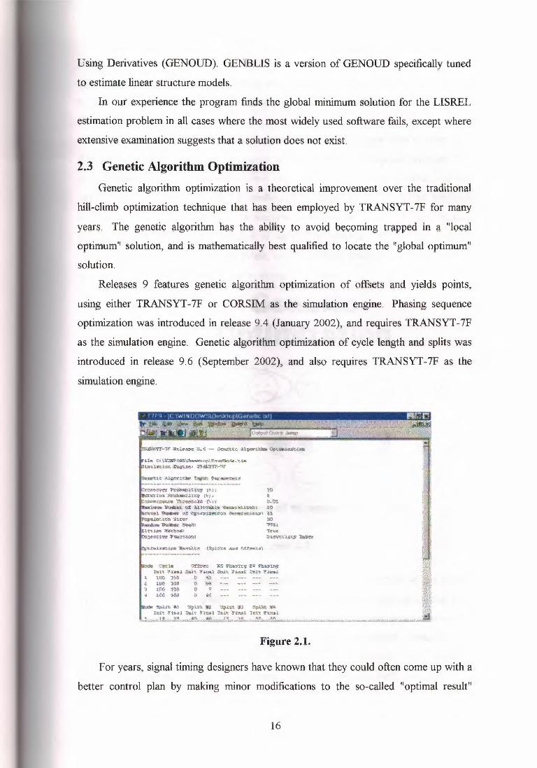
2.3 Genetic Algorithm OptimizationGenetic algorithm optimization is a theoretical improvement over the traditional
hill-climb optimization technique that has been employed by TRANSYT-7F for many
years, The genetic algorithm has the ability to avoid becoming trapped in a "local
optimum" solution, and is mathematicallybest qualified to locate the "global optimum"
solution.
Releases 9 features genetic algorithm optimization of offsets and yields points,using either TRANSYT-7F or CORSIM as the simulation engine. Phasing sequence
optimization was introduced in release 9.4 (January 2002), and requires TRANSYT-7F
as the simulation engine. Genetic algorithm optimization of cycle length and splits was
introduced in release 9.6 (September 2002), and also requires TRANSYT~7F as the
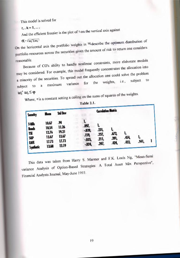
The nonlinear least squares problem has the general form
min{r(x): x E Ik" ı Where r is the function defined by r(x) = _.!._\\J(x)\\~ for some2
vector-valued function fthat maps R"toRm.
27
Least squares problems often arise in data-fitting applications. Suppose that some
physical or economic process is modeled by a nonlinear function ıp that depends on a
parameter vector x and time t. If bi is the actual output of the system at time r, , then the
residual </>( x, tJ - b, measures the discrepancy between the predicted and observed
outputs of the. system at time t; . A reasonable estimate for the parameter x may be
obtained by defining the ith component off by I, ( x) :::; t/)(x, t;) - b, ,
And solving the least squares problem with this definition off.From an algorithmic point of view, the feature that distinguishes least squares
problems from the general unconstrained optimization problem is the structure of the
Hessian matrix of r. The Jacobian matrix off, f'(x) = (aJ(x), ... .ô nf (x)) ,a be used to
express the gradient of r since Vr(x) = f '(x/ f (x). similarly, j'(x) is part of the
Hessian matrix V2r(x) sincem
V2r(x) = f'(x/ j'(x) + Lf;(x)V2J;(x).i=I
To calculate the gradient of r, we need to calculate the Jacobian matrixf'(x).
Having done so, we know the first term in the Hessian matrix V2r(x) without doing any
further evaluations. Nonlinear least squares algorithms exploit this structure.
In many practical circumstances, the first term f'(xl f'(x) in V2r(x) is more
importantthan the second term, most notably when the residuals t. (x) are small at the
solution. Specifically, we say that a problem has small residuals if, for all x near a
solution, the quantities\JJx)\\\v2 j;(x)\\, i = 1,2, ... ,n are small relative to the smallest
eigenvalue ofj'(xl f'(x).
• , Gauss-Newton Method
• Levenberg-Marquardt Method
• Hybrid Methods
• Large Scale Methods• Techniques for solving L.S. problems with constraints
• Notes and References
28
2.5 Global Optimization (GO)
A globally optimal solution is one where there are no other feasible solutions with
better objective function values. A locally optimal solution is one where there are no
other feasible solutions "in the vicinity" with better objective function values. You can
picture this as a point at the top of a "peak" or at the bottom of a "valley" ·which may be
formed by the objective function and/or the constraints -- but there may be a higher
peak or a deeper valley far away from the current point.
In certain types of problems, a locally optimal solution is also globally optimal.
These include LP problems; QP problems where the objective is positive definite (if
minimizing; negative definite if maximizing); and NLP problems where the objective is
a convex function (if minimizing; concave if maximizing) and the constraints form a
convex set. But most nonlinear problems are likely to have multiple locally optimal
solutions.
Global optimization seeks to find the globally optimal solution. GO problems are
intrinsically very difficult to solve; based on both theoretical analysis and practical
experience, you should expect the time required to solve a GO problem to increase
rapidly -- perhaps exponentially -- with the number of variables and constraints.
2.5.1 Complexity of the Global Optimization ProblemThe global optimization problem is indeed hard. Rinnooy Kan and Timmer [ 16]
claim that the global optimization problem is unsolvable in a finite number of steps.
Their argument is as follows:
For any continuously differentiable function f, any point S.and any neighborhood
B of .ı:,., there exists a functıio11tJ such that f + J is continuously differentiable, f + J equals f for all points outside B and the global minimum off+ J is s •. ((j + /) is an of
f) Thus, for any point s,., one cannot guarantee that it is not the global minimum
without evaluating the function in at least one point in every neighborhood B of s •. As
B can be chosen arbitrarily small, it follows that any method designed to solve the
global optimization problem would require an unbounded number of steps.
The indentation argument is certainly valid if one wishes to guarantee that an exact
poıimıt:., s., is a global mimmi~er. indeed, should the exact global minimieer be an
irrational number, it is obviously impossible, in a finite number of steps, to numerically.>
29
represent this solution. However, one can, in a finite amount of time, guarantee that
/(s.) =I~. . .IS Wilfüm
2.5.2 Solving GO Problems
Multistart methods are a popular way to seek globally optimal solutions with the
aid of a "classical" smooth nonlinear solver (that by itself finds only locally optimal
solutions). The basic idea behind these methods is to automatically start the nonlinear
Solver from randomly selected starting points, reaching different locally optimal
solutions, then select the best of these as the proposed globally optimal solution.
Multistart methods have a limited guarantee that (given certain assumptions about the
problem) they will "converge in probability" to a globally optimal solution. This
means that as the number of runs of the nonlinear Solver increases, the probability that
the globallyoptimal solution has been found also increases towards 100%.
Where Multistart methods rely on random samplingof starting points, Continuous
Branch and Bound methods are designed to systematically subdivide the feasible
region into successively smaller subregions, and find locally optimal solutions in each
subregion. The best of the locally optimally solutions is proposed as the globally
optimal solution. Continuous Branch and Bound methods have a theoretical guarantee
of convergence to the globally optimal solution, but this guarantee usually cannot be
realized in a reasonable amount of computing time, for problems of more than a small
number of variables. Hence many Continuous Branch and Bound methods also use
some kind of random or statistical samplingto improve performance.
Genetic Algorithms, Tabu Search and Scatter Search are designed to find
"good" solutions to nonsmooth optimization problems, but they can also be applied to
smooth nonlinear problems to seek a globally optimal solution. They are often effective
at finding better solutions than a "classic" smooth nonlinear solver alone, but they
usually take much more computing time, and they offer no guarantees of convergence,
or tests for having reached the globallyoptimal solution.
2.6 Nonsmooth Optimization(NSP)The most difficult type of optimization problem to solve is a nonsmooth problem
(NSP). Such a problem may not only have multiple feasible regions and multiple locally
optimal points within each region -- because some of the functions are non-smooth or~r
even discontinuous, derivative or gradient information generally cannot be used to
30
determine the direction in which the function is increasing (or decreasing). In other
words, the situation at one possible solution gives very little information about where to
look for a better solution.
In all but the simplest problems, it is impractical to exhaustively enumerate all of
the possible solutions and pick the best one, even on a fast computer. Hence, most
methods rely on some sort of random sampling of possible solutions. Such methods are
nondeterministic or stochastic -- they may yield different solutions on different runs,
even when started from the same point on the same model, depending on which pointsare randomly sampled.
2.6.1 Solving NSP Problems
Genetic or Evolutionary Algorithms offer one way to find "good" solutions to
nonsmooth optimization problems. (In a genetic algorithm the problem is encoded in a
series of bit strings that are manipulated by the algorithm; in an "evolutionary
algorithm," the decision variables and problem functions are used directly. Most
commercial Solver products are based on evolutionary algorithms.)
These algorithmsmaintain a population of candidate solutions, rather than a single
best solution so far. From existing candidate solutions, they generate new solutions
through either random mutation of single points or crossover or recombination of two
or more existing points. The population is then subject to selection that tends to
eliminate the worst candidate solutions and keep the best ones. This process is repeated,
generating better and better solutions; however, there is no way for these methods to
determine that a given solution,is truly optimal.I
Tabu Search and Scatter Search offers another approach to find "good" solutions
to nonsmooth optimization problems. These algorithms also maintain a population of
candidate solutions, rather than a single best solution so far, and they generate new
solutions from old ones. However, they rely less on random selection and more on
deterministic methods. Tabu search uses memory of past search results to guide the
direction and intensity of future searches. These methods generate successively better
solutions, but as with genetic and evolutionary algorithms, there is no way for these
methods to determine that a given solution is truly optimal.
31
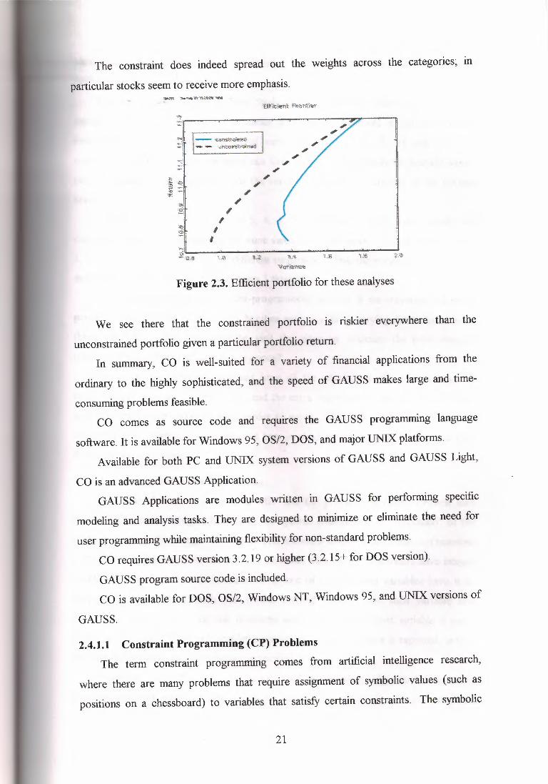
.7 Multi-Objective Optimization for Highway Management
Programming
Highway infi-astructwre is a major naıtioım:a[ investment, and a well-managed
highway network forms an integral element of a sustainable economy. An ideal
management program for a highway network is one that would maintain all highway
sections at a sufficientlyhigh level of service and structural condition, but requires only
a reasonably low budget and use of resources, without creating any significant adverse
impact on the environment, safe traffic operations, and social and community activities.
Unfortunately, many of these are conflicting requirements. For instance, more resources
and higher budgets may be needed if the highways are to be maintained at a high state
of operability. But this could lead to pavement activities causing longer traffic delays,
increased pollution, more disruption of social activities, and inconvenience to the
community. Therefore, the decision processes involved in highway management
activities requires a multi-objective consideration that addresses the competing
requirements of different objectives.
Practically all the pavement management-programming tools in use currently are
based on single-objective optimization. In single-objective analysis, the requirements
which are not incorporated into the objective function are imposed as constraints in the
formulation. This can be viewed as an interference of the optimization process, which
artificiallysets limits to selected problem parameters. As a result, the solutions obtained
from single-objectiveanalysis are sub-optimal with respect to one's derived from multiobjective formulations.
A genetic-algorithm (GA) based formulation for multi-objective programming of
highway management activities has been developed at the Centre for Transportation
Research. Genetic algorithms, which are a robust search technique formulated on the
principles of natural selection and natural genetics, are employed to generate and
identify-better solutions until convergence is reached. The selection of good solutions is
based on the so-called Pareto based fitness evaluation procedure by comparing the
relative strength of the generated solutions with respect to each of the adoptedobjectives.
An important aspect of multi-objective GA analysis is the definition of "fitness" of a
solution. The "fitness" of a solution directly influences the probability of the solution
being selected for reproduction to generate new offspring solutions. To overcome the
32
ore-mentioned problem, a rank-based fitness assignment scheme is used where all
non-dominated solutions in a given pool of solutions are assigned a rank of 1. Solutions
that are dominated by one solution will have a rank of 2, those dominated by two
solutions are given a rank of 3, and so on.
In the evaluation of a pool of solutions, one can identify a curve (for the case of
two-objective problems) or a surface (for the case three- or higher multi-objective
problems), which are composed of all non-dominated solutions. This curve or is known
as the Pareto frontier. The GA optimization process seeks to generate new solutions that
would give an improved frontier that dominates the existing frontier. This process
continues until, ideally, a set of globally non-dominated solutions is found. These
globally non-dominated solutions, called the Pareto optimal set, define the Pareto
optimal frontier.
The general procedure of GA operations and offspring generation in multi
objective programming is similar to that for single-objective programming. The main
difference lies with the evaluation of "fitness" of each solution, which is the driving
criterion of the search mechanism of genetic algorithms. An important consideration of
the optimization process is to produce representative solutions that are spread more or
less evenly along the Pareto frontier. This can be achieved by using an appropriate
reproduction scheme to generate offspring solutions and to form a new pool of parent
solutions.
The proposed procedure is illustrated by means of a highway maintenance
optimization problem at network level subject to five forms of resources and operation
constraints. The five constraints were production requirements, budget, manpower
availability, equipment availability, and rehabilitation schedule. The problem
considered four highway classes, four pavement defects and three levels of
maintenance-need urgency. Its objective was to select an optimal set of maintenance
activities for an analysis period of 45 working days.
The decision variables were the respective amounts of maintenance work,
measured in workdays, assigned to each maintenance treatment type. There were 48
treatment types referring to maintenance repairs arising from 4 distress forms of 3
maintenance-need urgency levels on 4 highway classes. The coded string structure of
GA representation thus consisted of 48 cells. Each cell could assume an integer value of<"
workdays from O to 45.
33
In this example, the following four objective functions were considered: (a)
minimization of the total maintenance cost; (b) maximization of overall network
pavement condition; (c) minimization of total manpower requirement, and (d)
maximizationof work production in total workday units. For the purpose of illustrating
the flexibilityof GAs in handling multi-objective problems, two different analyses were
performed. They consisted of a two-objective and a three-objective problem. The
objectives of the former were minimizationof total maintenance cost and maximization
of maintenance work production, while those of the latter were minimization of total
maintenance cost, maximization of maintenance work production, and maximization of
overall network condition.Figure 2.4 shows the convergence pattern of the Pareto frontier for the case with
two- objective problem. The convergence trend was apparent with the Pareto front
moving in the direction towards lower maintenance costs and higher maintenance work
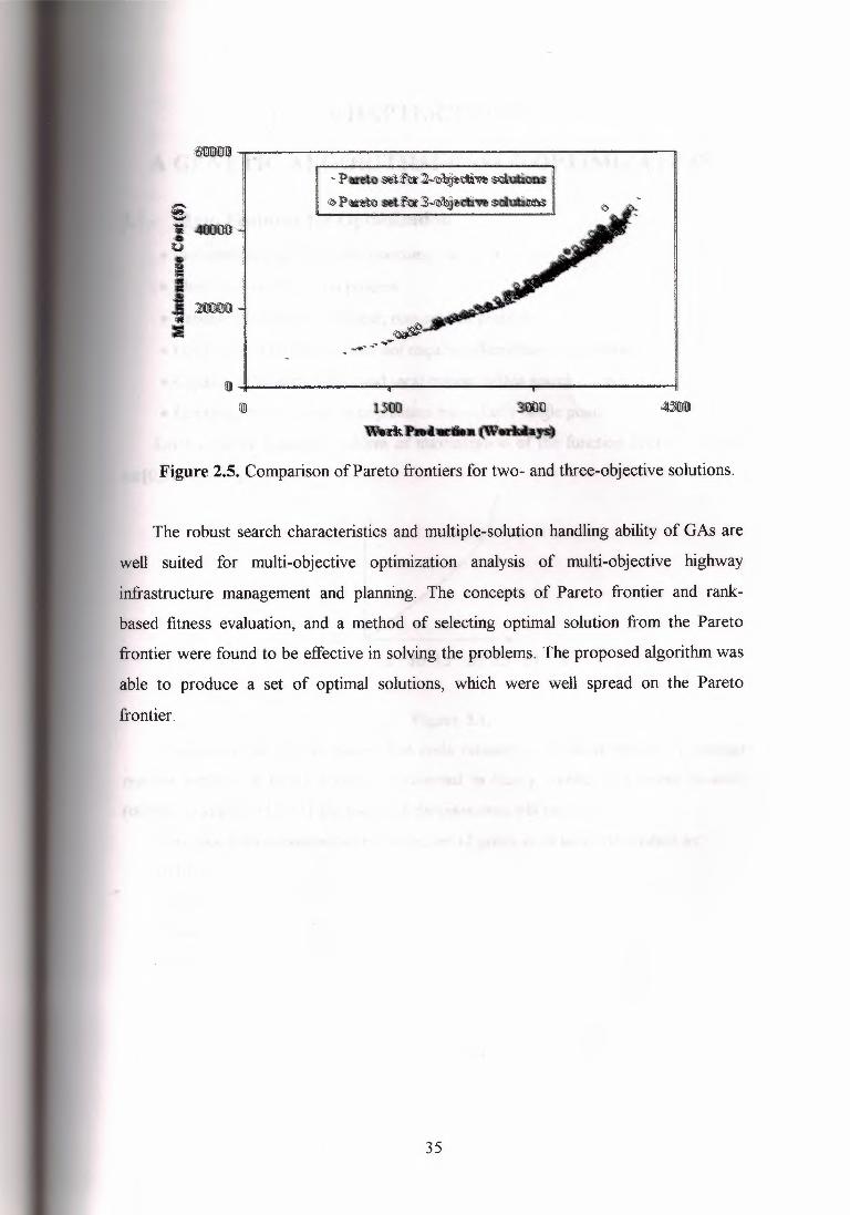
production. Figure2.5 presents the Pareto optimal frontiers of both the two-objective
and three-objective optimization solutions in the same two-dimensional plot of
(maintenance cost) vs. (work production) for comparison. It can be seen that although
the two Pareto frontiers are very close to each other, the Pareto frontier of the two
objective solutions appear to dominate the frontier of the three-objective solutions in
terms of maintenance cost and work production. This was clearly the effect of
introducing a third objective, i.e. maximizingpavement condition, in the three-objective
problem, in compromisingthe two initial objectives.
sİ 4[()1!IIOOu
I1500 )Q,1f!ij
w.t:Pıımırtiııll~
Figure 2.4. Convergence ofPareto frontier in GA Solutions
(A) All objectives except one are converted into constraints. The remaining
objective is maximized. The constraints are incremented and the model is run
iteratively. (B) All objectives are weighted and considered in the objective function
simultaneously.A different set of weights is used in each run.Alternatively, preference-based MO techniques, such as goal programming, may
require only a single optimization model run to identify the solution that best meets
prespecified "ideal" levels of each objective. Both classes of classical MO procedures
are discussed in detail by Cohon (1978).MO procedures have been used successfully within traditional mathematical
optimization procedures, such as linear programming, integer programming and
nonlinear programming. Many realistic problems, however, involve complex, nonlinear
relationshipsthat do not fit readily into one of these traditional frameworks.Recently, many such problems have been solved by employingnon-gradient-based,
probabilistic search techniques such as genetic algorithms (GAs) and simulated
annealing (SA). Both GA and SA may be used in the classical MO procedures.
However, the inherent parallel structure of a GA provides some important advantages in
MO analysis: with the appropriate schemes and operators, the population of solutions
carried in a GA can be directed to converge along the Pareto set in a single run. Several
multiobjective GA (MOGA) techniques that take advantage of this behavior are
summarizedin the following section.
47
The objective of this paper is to present a new method for MOGA, called the
neighborhood constraint method (NCM). NCM differs from previous MOGA
approaches by using a unique combination of a neighborhood selection technique and
location-dependent constraints. A description of NCM and its application to an
illustrative air quality management problem are provided. Performance of NCM is
compared with those of several other MOGA techniques, as well as with the
performance of a single-objective GA (SOGA) and an integer programming approach
using the classical MO constraint method.
3.3.2 Literature Review: GAs in Mo Analysis
In a review of multiobjective optimization techniques, Fonseca and Fleming (1995)
classify MOGA techniques into four major categories: plain aggregation methods,
population-based non-Pareto methods, Pareto-based approaches, and niche induction
schemes. Plain aggregation methods use GAs in classical MO procedures like those
depicted in Figure 3 .2. These methodologies do not take advantage of the GA
population-based search to generate the Pareto set in a single run, but instead require
much iteration.
The most well known population-based, non-Pareto method is the Vector
Evaluated Genetic Algorithm, or VEGA (Schaffer, 1991). In the VEGA scheme, the
population is divided into groups in each generation, and each group is evaluated with
only, a single objective. Individuals from different groups are allowed to mate with the
intent that offspring will perform well with respect to the objectives of both their
parents. While this approach and several of its variations have been successful in
locating the elbow and extreme points of the Pareto set, it is recognized that exploration
of the entire Pareto set is difficult..
In an intriguing non-Pareto technique, Hajela and Lin (1992) used a combination of
restrictive mating, objective weighting, and fitness sharing. Their variable weighting
approach treats the weights on objectives as decision variables that are encoded into the
GA chromosome for each individual. Combined with fitness sharing, this approach
allows individuals to evolve to represent a large number of different weightings.
Fleming and Pashkevich (1985) noted that any technique that aggregates objectives
linearly in the objective function, as in VEGA and Hajela and Lin's techniques, is not
capable of exploring concave regions of the Pareto set.
48
Pareto-based approaches were proposed by Goldberg (in 1989) and have become a
major focus of MOGA research. These techniques explicitly make use of the definition
of Pareto optimality. In Pareto schemes, the fitness of an individual is defined in terms
of rank. For each generation of the GA, the non-dominated set of solutions in the
population is given the top rank and then removed from that population. This step is
repeated, where in each iteration the non-dominated set of solutions remaining in the
population is given the next rank, until all solutions in the population are assigned a
rank. Rankings are then typically used in a tournament selection to encourage the
exploration in the direction of nondominated individuals.
Successful applications of this procedure have been reported by Cieniawski et al. (1995)
and Ritzel et al. (1994). Liepins et al. (1988) found the Pareto optimal ranking scheme
to be superior to VEGA An important advantage of Pareto approaches is that they are
able to identify solutions in concave areas of the Pareto set.
Pareto schemes typically suffer from population drift, where the population migrates to
a small portion of the Pareto set (Goldberg and Segrest, 1987). To assure a uniform
sampling of the Pareto set, recent applications of Pareto-based MOGA by Fonseca and
Fleming (1993), Horn et al. (1994), and Srinivas and Deb (1994) have incorporated
niching schemes.
In both the Pareto and niched-Pareto methods, there may be a likelihood of mating
between individuals that are far apart in the nondominated set. These solutions likely
will be very different in decision space, and as a result, their children may not meet
either objective satisfactorily (Goldberg, 1989). The niched-Parteto scheme by Fonseca
and Fleming (1993) and the non-Pareto scheme by Hajela and Lin (1992) deal with this
problem by restricting mating to individuals in similar regions in the objective space.
3.3.3 Neighborhood Constraint Method
Overview
· The Neighborhood Constraint Method (NCM) presented here is a MOGA technique
that:
• Samples effectivelyfrom along the entire Pareto set, includingthe endpoints
• Examines both convex and concave regions of the Pareto set, and
• Provides a computationally-efficientapproach
49
While MOGA techniques by Hom et al. (1994) and Fonesca and Fleming (1993)
also address these issues, NCM was developed concurrently and uses a very different
approach.NCM falls into the class of non-Pareto MOGA techniques because it does not make
explicit use of Pareto dominance in fitness evaluation. NCM is inspired by the natural
phenomena of adaptation to environmental conditions that are location ally, or
geographically, dependent (e.g. the gradual darkening of skin color seen in human
populations as one travels south from northern Europe to the equator). Adaptation, in
this case, arises either from the preferential selection of traits that perform well with
respect to the local environment, or through migration of traits to environments where
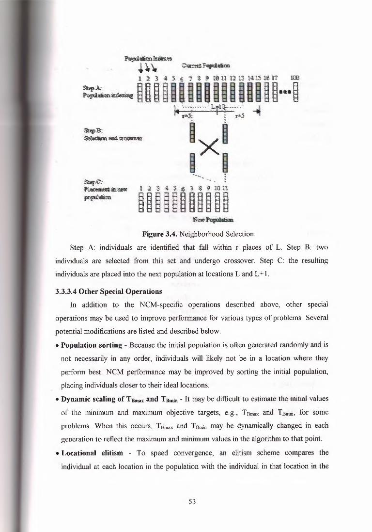
they are better suited.NCM includes the following major operations: population indexing, location-
dependent constraints, and restrictive mating using a neighborhood selection scheme.
These operations are described below.
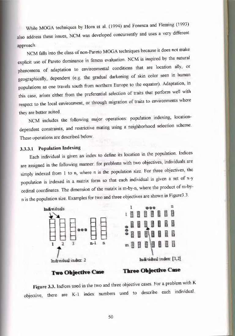
3.3.3.1 Population IndexingEach individual is given an index to define its location in the population. Indices
are assigned in the following manner: for problems with two objectives, individuals are
simply indexed from 1 to n, where n is the population size. For three objectives, the
population is indexed in a matrix form so that each individual is given a set of x-y
ordinal coordinates. The dimension of the matrix is m-by-n, where the product of m-by
n is the population size.Examples for two and three objectives are shown in Figure3.3.
İıtlııli-ıi~
i~~~~--·~··.~··l
ı I I RD IiD. o• I\ I .s I U> I·····.· ·'~ I· I u:.:ı Di I" O#itft. Bi 6 B . Bi ilO
ıttı~¥.~~itı~: •. [~~j····
-~iöıaJedhreC•
Figure 3.3. Indices used in the two and three objective cases. For a problem with K
objective, there are K-1 index numbers used to describe each individual.
50
For problems of four or more objectives, individuals are indexed in a similar fashion,
with the number of index values set equal to the number of objectives minus I.
3.3.3.2 Location-Dependent Constraints
NCM handles multiple objectives in a very similar manner to the classical
MO constraint method. For a K-objective problem, K-1 objectives are converted into
constraints while the remaining objective is optimized. What makes this method unique
is that the values of the constrained objectives are gradually varied at each index
location in the population.
Consider the two-objective problem with objectives A and B and a
population size of n. The individual with index I would be constrained to satisfy
objective B at a minimumtarget level TBrnin- The individualwith index n would instead
be constrained to a maximum target level TBmax- The constraint for any individual i in
the population is generalizedby:
Conversion of these targets to constraints in the GA is done through the use of
penalties. Although the form of the penalty function may be problem specific, it
generallycan be incorporated in the fitness function as:
Where: C is the total cost; Aj is the cost at source i. Cj,t is the binary variable
representing whether control option tis used at source j; Uj is the emissions at source j;
ej,t is the removal efficiencyof control t at source j, and T is the target level of emissions
reduction. The problem is described in more detail by Laughlin (1995).
This problem can be modeled and solved as an integer programming (IP)
formulation, allowing the comparison of the GA results with the actual Pareto otimal
solutions obtained using the IP. Also, this problem is closely related to another
formulation that we have been examining in our research, in which a highly nonlinear
air quality model is used in the eyaluation function to predict air quality impacts. This
alternative GA formulation seeks to minimize costs subject to an ambient air quality
constraint. The complexity of the atmospheric transport and chemistry makes the use ofmore classical intractable.optimization methodologies
Also, because of the duration of an atmospheric model run, the efficiency and
quick convergence of a MOGA technique are important, providing the impetus for thework presented in this paper.
55
3.3.4.1 Methodology
Four MO methods were tested and compared for the case study problem. Eachmethod is 'describedbriefly.
1. Integer Programming
First, an integer-programming (IP) model was set up and solved to determine the
true Pareto optimal costs for achieving emissions reductions of 5%, 10%, 15%, 20%,
25%, 30%, 35%, 40%, 45%, 50%, and 55%. The IP model contained approximately1300 binary decision variables.
2. Single-Objective GA
Next, a single-objective GA (SOGA) was run iteratively, one run for each level of
reduction, i.e. 5%, 10%, etc. The SOGA, as well as the MOGA techniques tested in this
paper, used real-coded genes. Coding of the decision variables is discussed by Laughlin(1995).
Other parameters used in the SOGA runs included: a mutation rate of O. 1 %, a
uniform crossover rate of 35%, tournament selection, and elitism to preserve the best
individual in each generation. 30% of genes that underwent crossover were subjected to
a linear recombination. These parameter values were found to perform well through
trials of various parameterizations. Population sizes of 50 and 150 individuals were
tested, each for 15 different random number seeds. The runs were terminated when no
improvement in fitness was observed in 20 consecutive generations.
3. The Neighborhood Constraint Method
NCM was then used to generate the tradeoff curve in a single run. The NCM
specificparameters used in this problem are listed in Table 3.4.
i;~~~~:ı
56
For NCM, only 10% of the genes that underwent crossover were linearly
recombined. While this value may appear low, trials suggested that a low value allowed
for better gene migration across the population with less chance of disruption.
Once again, runs were made for population sizes of 50 and 150 individuals for 15
different random number seeds. Termination occurred after 20 generations with no
improvement in the average cost of individuals in the population.
Pareto Ranking and Hybrid Niched-Pareto MOGAs
Pareto ranking and a hybrid niched-Pareto MOGA technique were implemented
and tested for the same population sizes and random seeds. The Pareto ranking scheme
was based on the procedure described by Goldberg (1989).
The hybrid technique was a combination of two techniques described in the literature,and made use of
• Objective sharing - Combined with tournament selection, this technique
encouraged exploration of the tradeoff curve by promoting selection of individuals
in relatively nonpopulated areas. The objective sharing implementation was basedon the procedure described by Horn et al. (1994).
• Restrictive mating - This technique, adapted from Fonseca and Fleming (1993),
used a parameter, mating, to encourage the mating of individuals that are similar inobjective space.
Tournament selection was used in this hybrid method. A number of individuals
equal to 10% (arbitrarily chosen) of the population size was sampled. If there was a tie
in the ranking of the best individuals in the sample, continuously- updated objective
sharing was used to identify the winner, as described by Horn et al. (1994). Another
samplingof roughly 10% of the population was taken to find a mate. After the sampling
was completed, the new set of individuals was evaluated to determine whether the
individuals fell within an objective-space distance, mating, from the winner of the first
tournament. The fitness of individuals that fell within this distance was increased to
encourage selection. If there was a tie, objective sharing was carried out in the secondsampled set to identifythe mate.
57
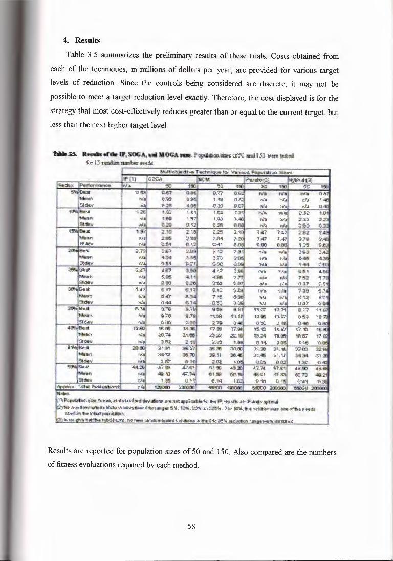
4. Results
Table. J.5 summarizes the preliminary results of these trials. Costs obtained from
each of the techniques, in millions of dollars per year, are provided for various target
levels of reduction. Since the controls being considered are discrete, it may not be
possible to meet a target reduction level exactly. Therefore, the cost displayed is for the
strategy that most cost-effectively reduces greater than or equal to the current target, but
less than the next higher target level.
Results are reported for population sizes of 50 and 150. Also compared are the numbers
of fitness evaluations required by each method.
58
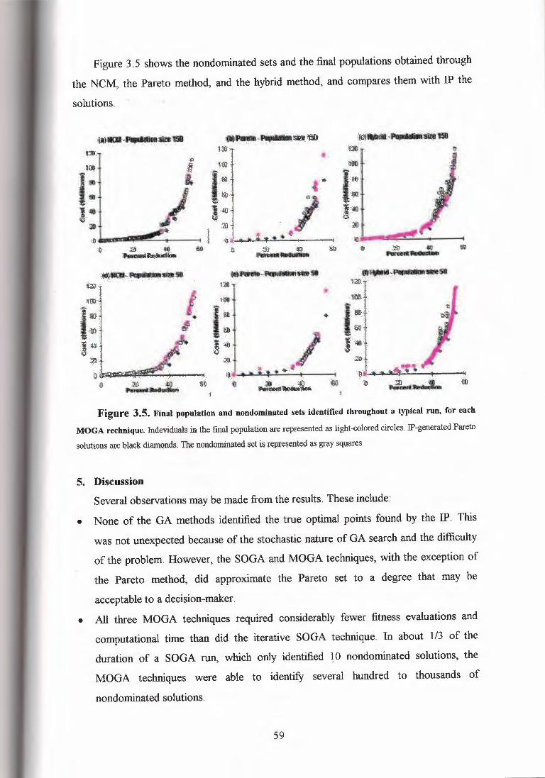
Figure 3. 5 shows the nondominated sets and the final populations obtained through
the NCM, the Pareto method, and the hybrid method, and compares them with IP the
solutions.
iiı~:o
.•. ,,,y-·r~•~
•J®Y~~~••• 5:,ı
O;~'-~)- )n ~~~~ ~~• ıtı·•
.<r/
.. tın·· ~~~
Figure 3.5. Final population and nondominated sets identified throughout a typical run, for each
MOGA rechnique. Indeviduals in the final population are represented as light-colored circles. IP-generated Pareto
solutions are Plack diamonds. The noııdominated set is represented as gray squares
5. DiscussionSeveral observations may be made from the results. These include:
• None of the GA methods identified the true optimal points found by the IP. This
was not unexpected because of the stochastic nature of GA search and the difficulty
of the problem. However, the SOGA and MOGA techniques, with the exception of
the Pareto method, did approximate the Pareto set to a degree that may be
acceptable to a decision-maker.
• All three MOGA techniques required considerably fewer fitness evaluations and
computational time than did the iterative SOGA technique. In about 1/3 of the
duration of a SOGA run, which only identified l O nondominated solutions, the
MOGA techniques were able to identify several hundred to thousands of
nondominated solutions.
59
• The Pareto method found better solutions near the elbow region of the curve,
compared to the hybrid, NCM, and SOGA The results suggest that the Pareto
technique was superior at the elbow because it tended to direct more search effort in
that region than did the NCM and hybrid.
• Of the MOGA runs, the hybrid technique, with a population size of 150, identified
the best-nondominated solutions (Fig.3.5 c.f); providing good coverage of the entire
curve. However, the hybrid technique was more dependent on the random number
seed than NCM, and in several runs failed to identify solutions in the lower portion
of the tradeoff curve. Although the hybrid technique was able to find good
nondominated solutions, it was unable to maintain them throughout the search. The
final population tended to converge toward the elbow. NCM was able to cover the
noninferior set well, and also maintained the nondominated solutions throughout the
search (Fig.3.5 a, d). This behavior may be desirable because it reduces the book
keeping required to maintain records of solutions along the set. The Pareto
technique did poorly in covering the noninferior set and maintaining the
nondominated solutions.
• NCM exhibited better coverage of the Pareto set than the hybrid technique for runs
where the population was 50.
3.3.5 Summary
This paper presents a new multiobjective genetic algorithm technique, the
neighborhood constraint method (NCM). NCM uses a restrictive mating scheme and
location-dependent constraints to promote and maintain diversity in the GA population.
The application of the NCM technique to a realistic problem was demonstrated and
its performance was compared with those of an integer programming procedure, an
iterative procedure using a single-objectiveGA optimization, and a Pareto and a hybrid
niched-Pareto multiobjectiveGA (MOGA) techniques.
Preliminary results show that NCM performs better than the SOGA and the other
MOGA techniques. NCM appears to provide good coverage of the Pareto set, and is
capable of promoting and maintainingpopulation diversity throughout the GA run with
a relatively small population size. It does appear, however, that the Pareto-based
techniques may be better at identifying regions near the elbow of the Pareto set.
60
These results suggest that NCM is a viable MOGA technique, and point to the need
for a more comprehensive investigation of NCM to better identify the effects of the
restrictive mating and the location-dependent constraints. A determination of the best
selection approach (i.e., roulette wheel, tournament, etc.), selection radius, and
recombination and crossover rates to use with NCM would be beneficial. NCM should
also undergo a more rigorous comparison with the other MOGA techniques for a set of
well-known problems.
Another potential use of NCM that deserves attention is in parallel GAs, since the
methodology adapts well to -the decentralized selection schemes discussed by De Jongand Sarma (1995).
61
CONCLUSION
A couple of conclusions from building block theory are of importance to note.
Strings with very fit schemata of short length will have a high likelihood of being selected
to create the next population, and thus pass on those schemata to strings in the new
population. It has been shown that schemata of this form increase in number from one
population to the next in an exponential fashion. In other words, n3 useful schemata are
processed per generation, and the majority of these have small orders and lengths
associated with them. These schemata are what give a GA the power to efficiently search
through a-problem space. This n3 feature is so important to GAs that it has been given a
special name, implicit parallelism.If the conception of a computer algorithms being based on the evolutionary of
organism is surprising, the extensiveness with which this algorithms is applied in so manyareas is no less than astonishing. These applications, be they commercial, educational and
scientific, are increasingly dependent on this algorithms, the Genetic Algorithms. Its
usefulness and gracefulness of solving problems has made it the more favorite choiceamong the traditional methods, namely gradient search, random search and others. GAs are
very helpful when the developer does not have precise domain expertise, because GAs
possess the ability to explore and learn from their domain.In this project, the use of operators of GAs in optimization of engineering and
commerce are considered. We believe that, by these interesting examples, one could grasp
the idea of GAs with greater ease. The different optimization problems are described. The
application of GA to solve optimization problem are given the selection procedure modelparameters by using GA operators are represented. Also different problems solution, by
using GA, is given.In future, the developments of variants of GAs to tailor for some very specific tasks
will be interesting. This might defy the very principle of GAs that it is ignorant of the
problem domain when used to solve problem.But we would realize that this practice could
make GAs even more powerful
62
REFERENCES
[1] Water Resources Research, Cieniawski, S. E., Eheart, J. W., and Ranjithan, S.
(1995).[2] Genetic Algorithms in Engineering and Computer Science, edited by G.Winter,
J.Periaux& M.Galan, publishedby JOHN WILEY & SON Ltd. in 1995.
[3] [Louis 1993] Genetic Algorithms as a Computational Tool/or Design, by Sushil J_
Louis, in August 1993
[4] Algorithms and Complexity, by Herbert S.Wilf, in 1986 publishedby Prentice-Hall
Inc.Obtained: Central Library oflmperial College (3 Computing 5.25 WIL)
[5] Proceedings of the Sixth International Conference on Genetic Algorithms, De
Jong, K. A and Jayshree Sarma (1995).[6] Recombination Variability and Evolution: algorithms of estimation and
population-genetic models, by AB.Korol, I.A.Preygel & S.I.Preygel, in 1994 published
by Chapman& Hall.Obtained: Central Library of Imperial College (4 Life Sciences575.116.12 KOR)
[7] Learning Robot Behaviours using Genetic Algoeithms, bv ALAN C.Schultz. Na
Center for AppliedResearch in ArtificialIntelligneee
[8] Genetic Algorithms for Order Dependent Proa:s:ses tlJJPlied to Robot Path-
Planning, by Yuval Davidor, in April 1989 publishedby I:nperial College
[9] Genetic Algorithms in Business and Their SııpptWıi•ıe Role in Decision Makin
by Tom Bodnovich, in 16 November 1995, pı;.,ı-->Esbed by College of Business