Page 1
Near Maximum Likelihood Sequential
Search Decoding Algorithms for
Binary Convolutional Codes
Shin-Lin Shieh
Directed by: Prof. Po-Ning Chen and Prof. Yunghsiang S. Han
Department of Communications Engineering,
National Chiao-Tung University
June 19, 2008
1
Page 2
Outline
• Introduction
• Sequential Decoding Algorithms & Fano Metric
• MLSDA and the Proposed Early Elimination Scheme
• Performance Analysis & Window Size with Negligible Performance
Degradation
• Decoding Complexity Analysis
• Concluding Remarks
2
Page 3
Chapter 1 :
Introduction
3
Page 4
Viterbi decoding
• The most popular decoding algorithm for convolutional codes
• Decoding complexity increases exponentially with respect to the code
constraint length
• Limited to constraint lengths of 10 or less
• When the information length is long, path truncation in practical decoder
design
– majority vote strategy
– best state strategy
– random state (fixed state) strategy
4
Page 5
• Best state strategy is commonly used
– Forney (1974) proved using random coding argument that a truncation
window of 5.8-fold of the constraint length in enough
– Hemmati & Costello (1977) derived performance bound as a function of the
truncation window for a specific convolutional encoder and obtained a similar
conclusion
5
Page 6
Sequential decoding (stack algorithm)
• The sequential decoding (stack algorithm or ZJ algorithm) was introduced by
Zigangirov in 1966 and Jelinek in 1969
• Decoding complexity is almost irrelevant to the code constraint length.
Suitable for convolutional codes with memory order 12, 16, or even higher
• After the development of the Viterbi algorithm in 1967, sequential decoding
received little attention during the past 30 years due to its sub-optimum
performance and lack of efficient hardware implementation
• New application (Heegard 2003): Channel equalization of “super-code”
considering the joint effect of multi-path channel & convolutional code
6
Page 7
• Maximum-Likelihood Sequential Decoding Algorithm (MLSDA) :
– proposed by Han, Chen, and Wu in 2002
– change the decoding metric
– achieve maximum-likelihood performance
– decoding complexity considerably lower than Viterbi algorithm for medium to
high SNRs from a software implementation standpoint
– operate in trellis rather than tree due to the implementation of closed stack
7
Page 8
Modification of MLSDA decoding
• Directly eliminate the top path with small level compared with the farest
explored node
�� �
• Provide timely output (elimination:∆, decision:5 × (m + 1))
8
Page 9
Performance & complexity analysis
• Level threshold ∆ introduces a tradeoff between performance and complexity
• Analyze the smallest ∆ value with negligible performance degradation
– BSC: (random coding argument)
∗ 2.2-fold constraint length for rate 1/2
∗ 1.2-fold constraint length for rate 1/3
– AWGN: (specific encoder)
∗ 3-fold constraint length for rate 1/2
∗ 2-fold constraint length for rate 1/3
• Analyze the decoding complexity using the large deviations technique & the
Berry-Esseen theorem to find out how much decoding effort we can at least
save
9
Page 10
Chapter 2 :
Convolutional Codes &Stack Algorithm with Fano Metric
10
Page 11
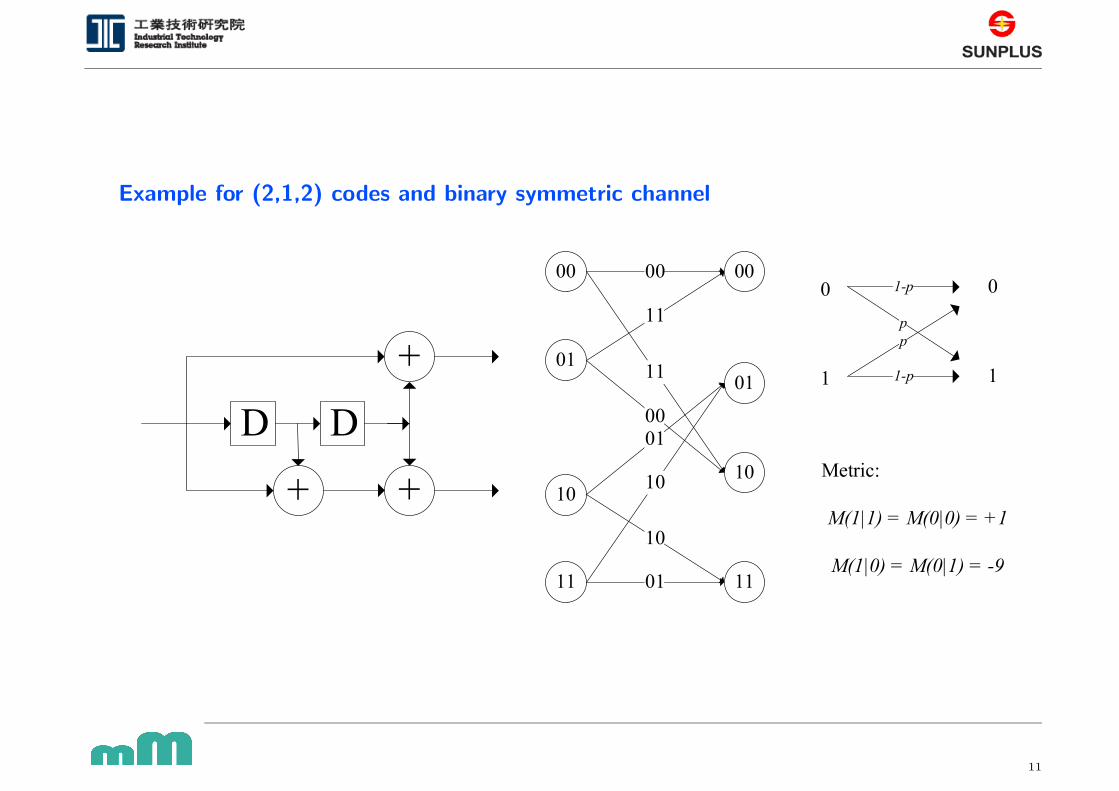
Example for (2,1,2) codes and binary symmetric channel
�� �
�
�
�� �
� � �� �� � � � � � � � � � �
� � �� � � � � � � �� � � � �
11
Page 12
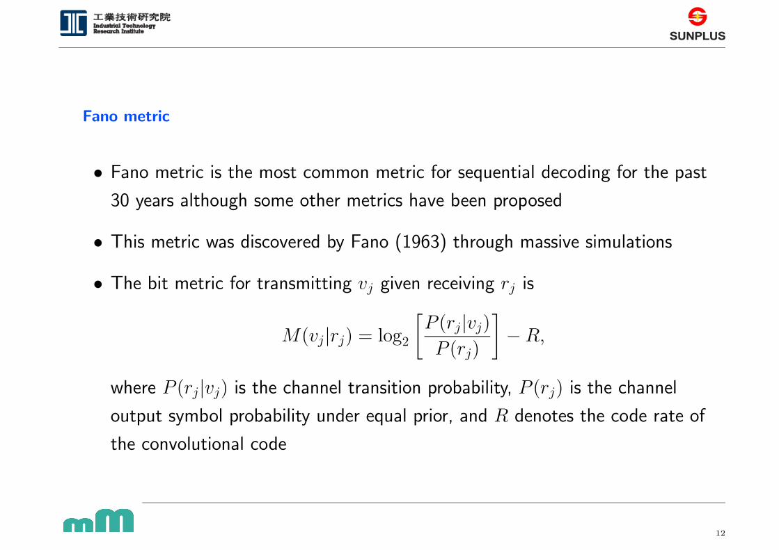
Fano metric
• Fano metric is the most common metric for sequential decoding for the past
30 years although some other metrics have been proposed
• This metric was discovered by Fano (1963) through massive simulations
• The bit metric for transmitting vj given receiving rj is
M(vj|rj) = log2
[
P (rj|vj)
P (rj)
]
− R,
where P (rj|vj) is the channel transition probability, P (rj) is the channel
output symbol probability under equal prior, and R denotes the code rate of
the convolutional code
12
Page 13
• For example, under Binary Symmetric Channel (BSC) with crossover
probability p,
M(vj|rj) =
log2(1 − p)+1 − R , for vj = rj;
log2(p)+1 − R , for vj 6= rj.
For code rate R = 1/2 and crossover probability p = 0.045,
M(vj|rj) =
0.434 , for vj = rj;
−3.974 , for vj 6= rj,
which can be scaled to
M(vj|rj) =
0.434 × 2.30415 ≈ 1 , for vj = rj;
−3.974 × 2.30415 ≈ −9 , for vj 6= rj.
• Note that Fano metric can be positive or negative!
13
Page 15
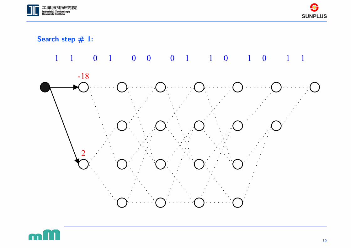
Search step # 1:
15
Page 16
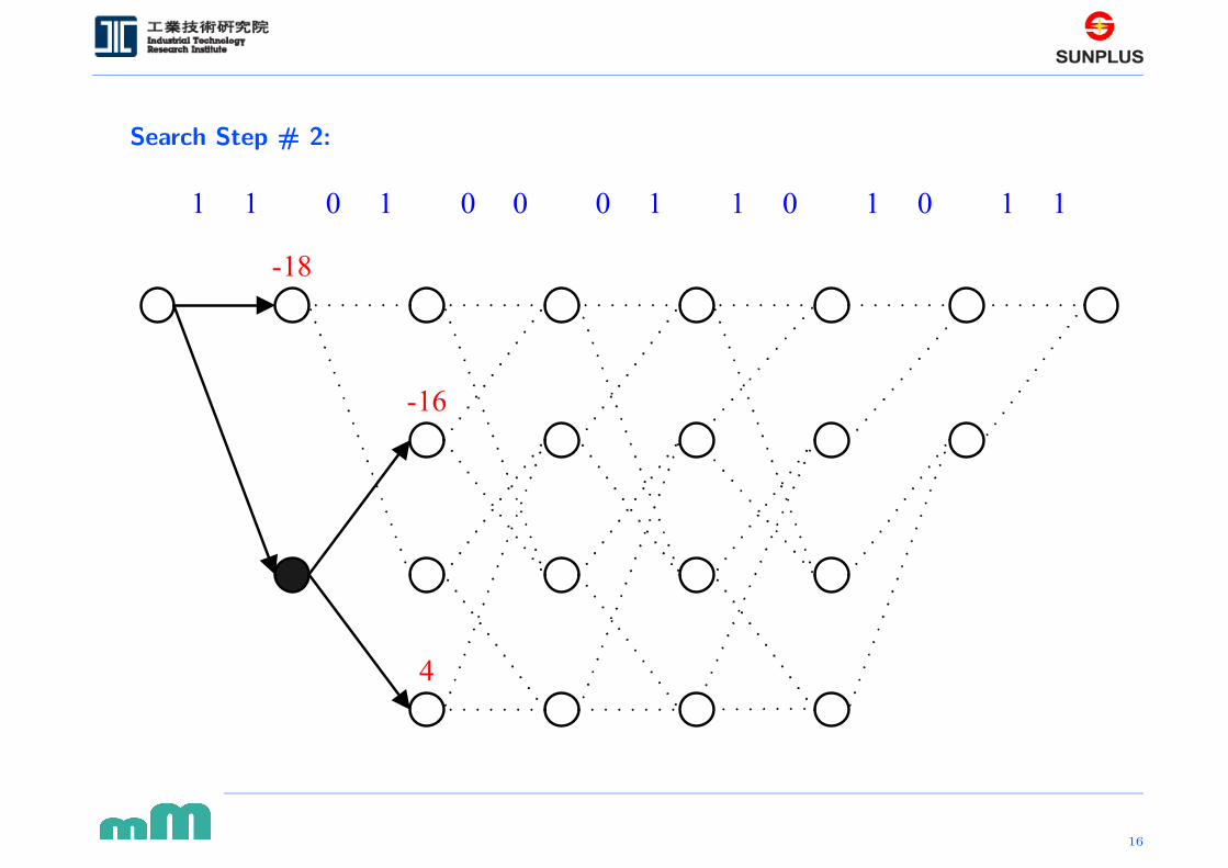
Search Step # 2:
16
Page 17
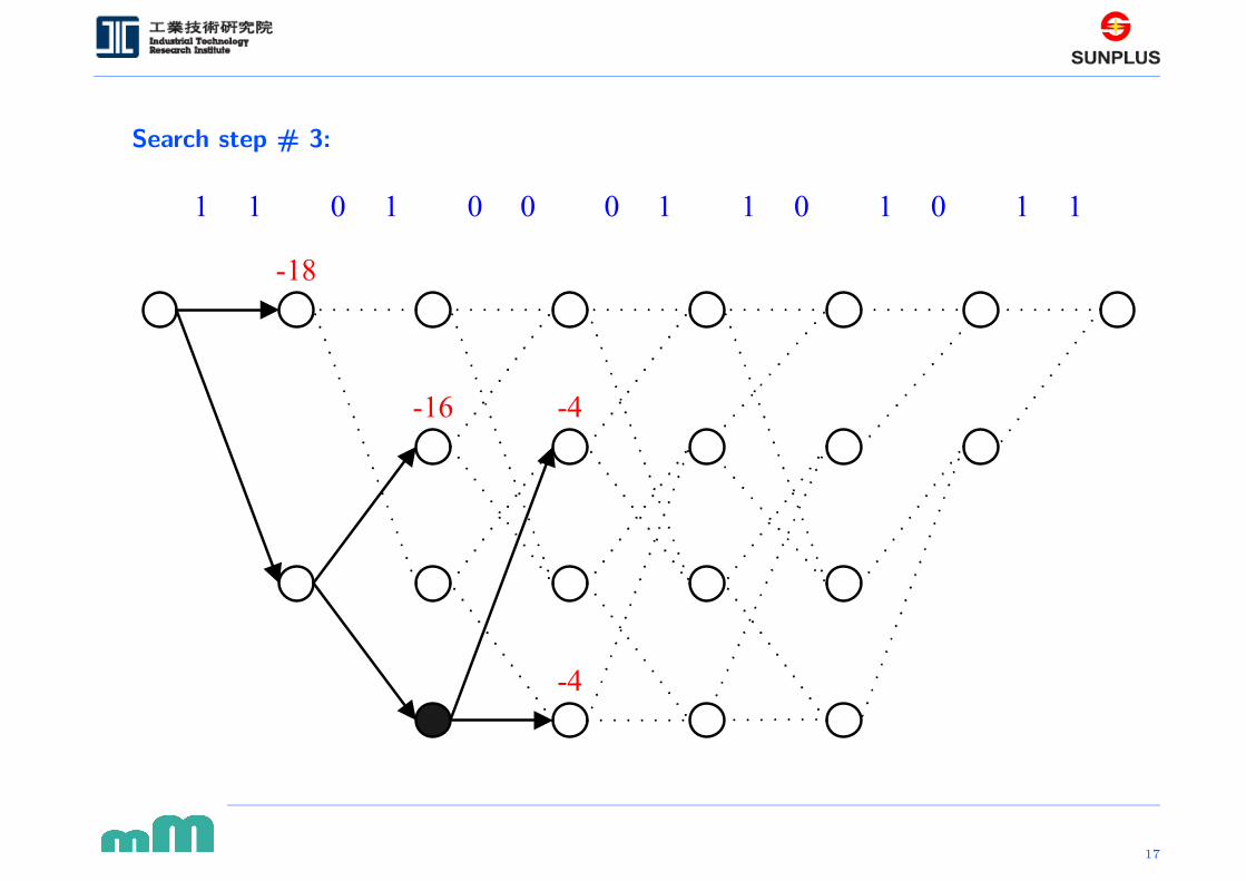
Search step # 3:
17
Page 18
Search step # 4:
�� �
� � � � � � � � � � � � � � � � � � � � � � � � � � � � � � � � � � � � � � � � � � � � � � � � � � � � � � � � � � � � � � � � � � � � � � � � � � � � � � � � � � � � � � � � � � � � � � � � � � � � � � �
�� � ��
�� �
��
18
Page 19
Search step # 5:
�� �
� � � � � � � � � � � � � � � � � � � � � � � � � � � � � � � � � � � � � � � � � � � � � � � � � � � � � � � � � � � � � � � � � � � � � � � � � � � � � � � � � � � � � � � � � � � � � � � � � � � � � � �
�� � ��
�� �
�� �
�� �
19
Page 20
Search step # 6:
�� �
� � � � � � � � � � � � � � � � � � � � � � � � � � � � � � � � � � � � � � � � � � � � � � � � � � � � � � � � � � � � � � � � � � � � � � � � � � � � � � � � � � � � � � � � � � � � � � � � � � � � � � �
�� �
�� �
�� �
�� �
�� �
�� �
20
Page 21
Search step # 7:
�� �
� � � � � � � � � � � � � � � � � � � � � � � � � � � � � � � � � � � � � � � � � � � � � � � � � � � � � � � � � � � � � � � � � � � � � � � � � � � � � � � � � � � � � � � � � � � � � � � � � � � � � � �
�� �
�� �
�� �
�� �
�� �
�� �
21
Page 22
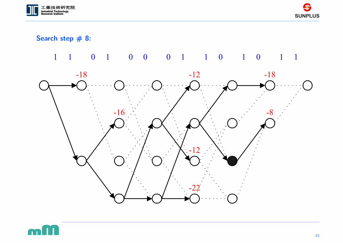
Search step # 8:
�� �
� � � � � � � � � � � � � � � � � � � � � � � � � � � � � � � � � � � � � � � � � � � � � � � � � � � � � � � � � � � � � � � � � � � � � � � � � � � � � � � � � � � � � � � � � � � � � � � � � � � � � � �
�� �
�� �
�� �
��
�� �
�� �
22
Page 23
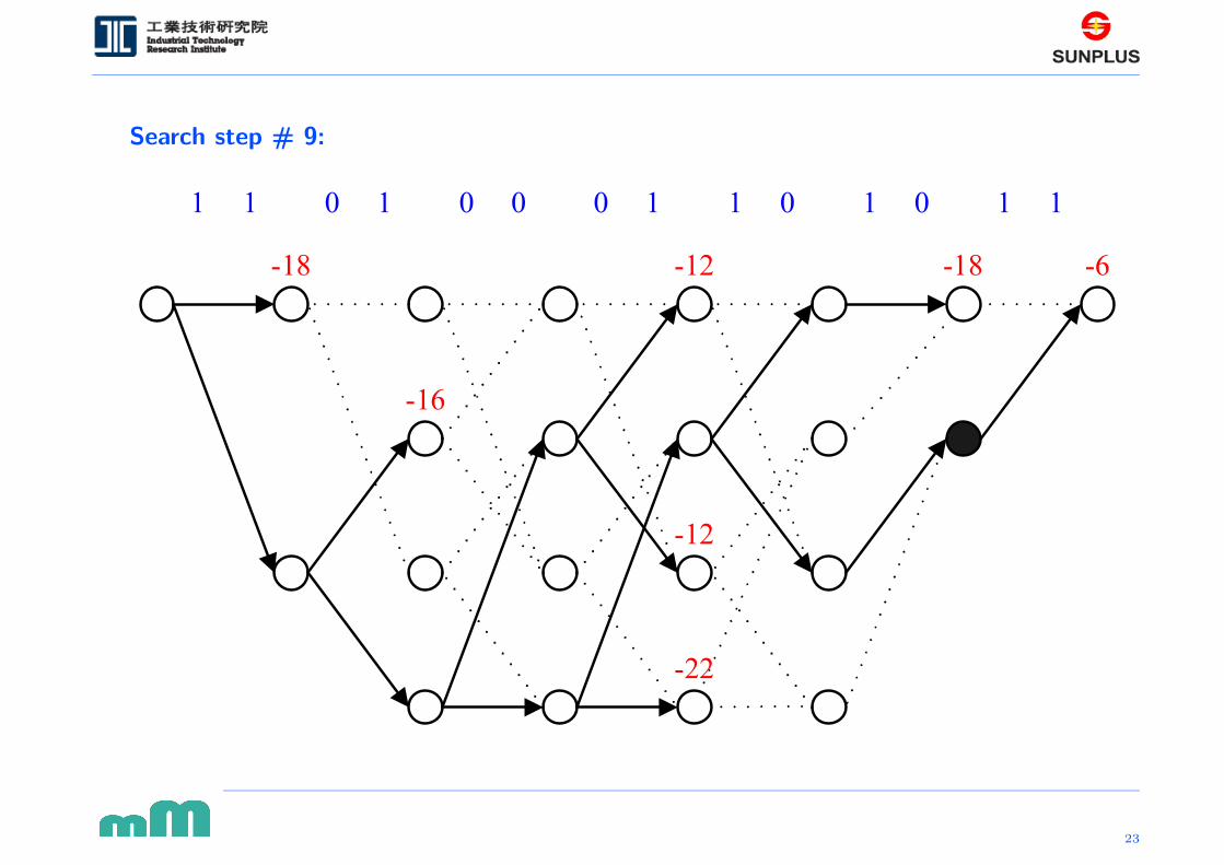
Search step # 9:
23
Page 24
Final Output
�������������������������������������������������������������������������������������������������������
24
Page 25
Sub-optimality
• Massey (1972) proved that extending path with largest metric minimize the
probability that the extending path does not belong to the optimal path
• However, not always guarantee the finding of the global optimal path since
the Fano metric may be positive
25
Page 26
Come back from behind due to positive metric?
26
Page 27
Performance with Fano metric (no quantization, no time out, perfect SNR est.)
1 1.5 2 2.5 3 3.5 4 4.5 510
−6
10−5
10−4
10−3
10−2
10−1
Eb / N
0
Bit
Err
or R
ate
(2,1,6) Viterbi(2,1,6) Sequential(2,1,12) Viterbi(2,1,12) Sequential
27
Page 28
Performance with Fano metric (quantization)
1 1.2 1.4 1.6 1.8 2 2.2 2.4 2.6 2.8 310
−6
10−5
10−4
10−3
10−2
10−1
100
Eb / N
0
Bit
Err
or R
ate
(2,1,16), Message Length 100
BER Fano Metric Q=3BER Fano Metric Q=4BER Fano Metric Q=5BER MLSDA Q=3BER MLSDA Q=4BER ML Q=∞
28
Page 29
Complexity with Fano metric (code tree)
1 1.5 2 2.5 3 3.5 4 4.5 510
0
101
102
Eb / N
0
Ave
rage
Dec
odin
g C
ompl
exity
Per
Info
rmat
ion
Bit
(2,1,6)(2,1,12)
2.70 cf. (2,1,6) Viterbi = 128
3.21 cf. (2,1,12) Viterbi = 8192
29
Page 30
Chapter 3 :
MLSDA &Early Elimination Scheme
30
Page 31
Novel metric with ML performance & low complexity
• Han, Chen, and Wu (2002) derived another metric based on the Wagner rule
• The path metric is defined as
µ(xj) , (yj ⊕ xj)|φj|,
where φj is the log-likelihood ratio, yj is the hard decision and xj is the
encoder output
• This metric is non-negative. It was proved that the metric is a
maximum-likelihood metric
31
Page 32
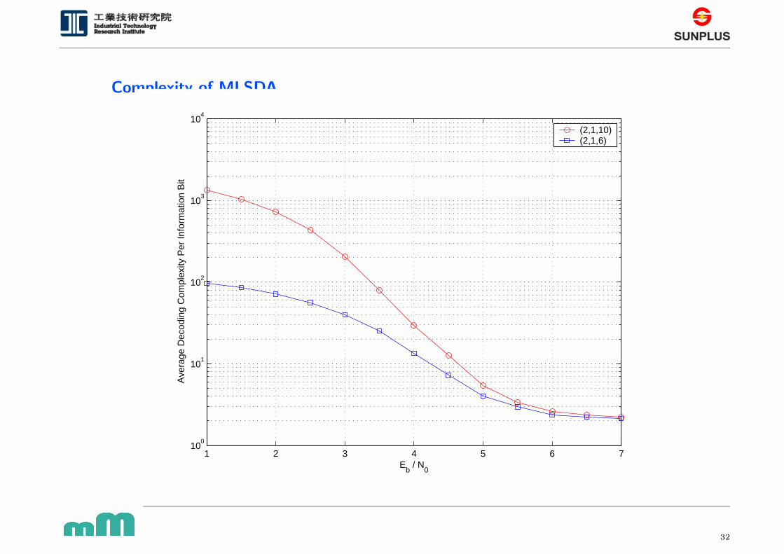
Complexity of MLSDA
1 2 3 4 5 6 710
0
101
102
103
104
Eb / N
0
Ave
rage
Dec
odin
g C
ompl
exity
Per
Info
rmat
ion
Bit
(2,1,10)(2,1,6)
32
Page 33
Average decoding complexity per information bit of MLSDA
50 100 150 200 250 300 35010
1
102
103
Message Length
Ave
rage
Dec
odin
g C
ompl
exity
Per
Info
rmat
ion
Bit
(2,1,10) Codes, AWGN, Eb/N
0 = 3.5 dB
33
Page 34
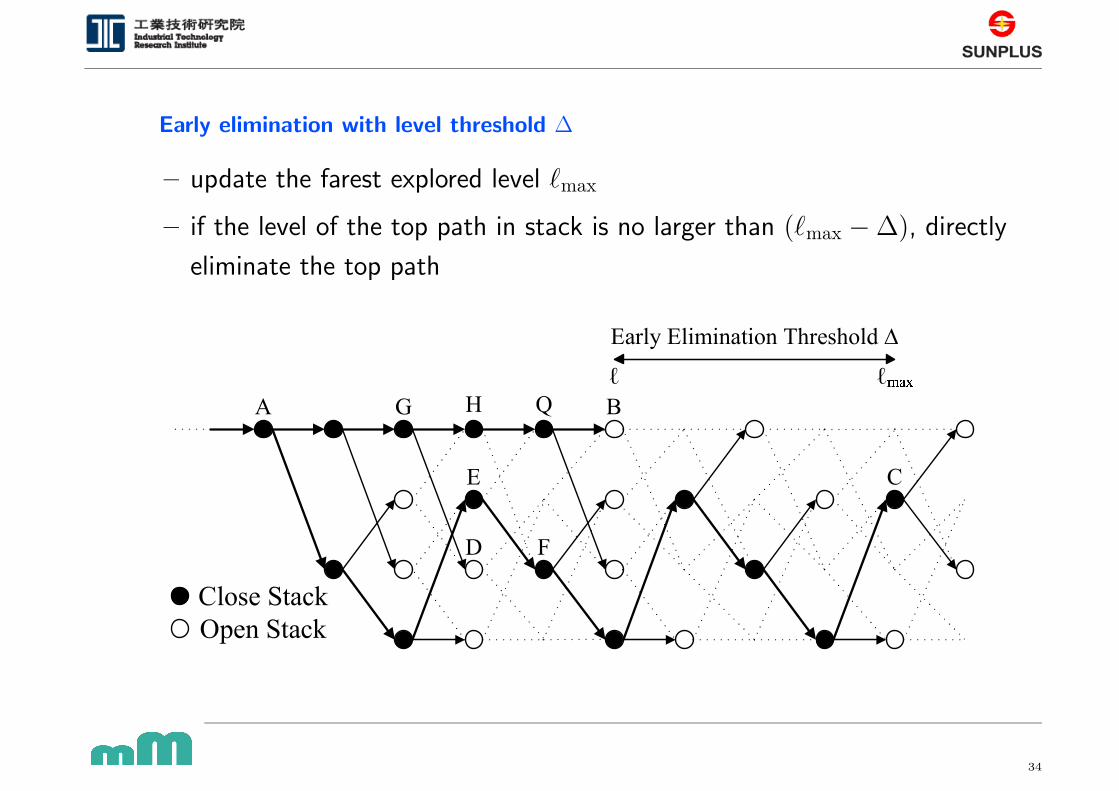
Early elimination with level threshold ∆
– update the farest explored level `max
– if the level of the top path in stack is no larger than (`max − ∆), directly
eliminate the top path
�� �
34
Page 35
Chapter 4 :
Random Coding Argument &Performance Analysis for BSC channel
35
Page 36
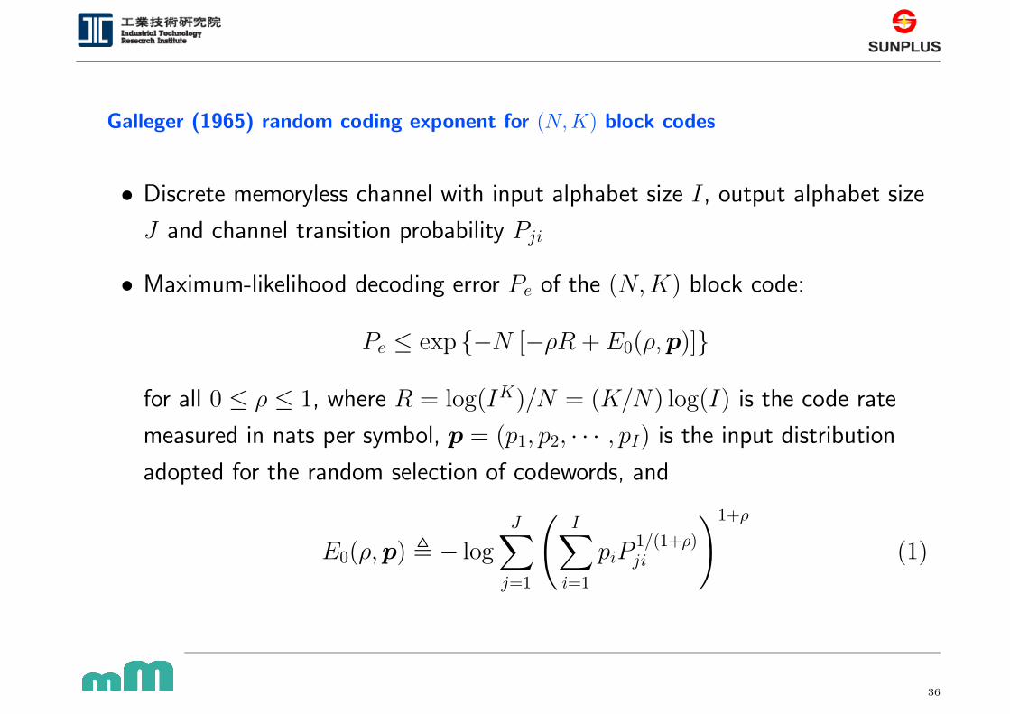
Galleger (1965) random coding exponent for (N, K) block codes
• Discrete memoryless channel with input alphabet size I, output alphabet size
J and channel transition probability Pji
• Maximum-likelihood decoding error Pe of the (N, K) block code:
Pe ≤ exp {−N [−ρR + E0(ρ, p)]}
for all 0 ≤ ρ ≤ 1, where R = log(IK)/N = (K/N) log(I) is the code rate
measured in nats per symbol, p = (p1, p2, · · · , pI) is the input distribution
adopted for the random selection of codewords, and
E0(ρ, p) , − logJ∑
j=1
(
I∑
i=1
piP1/(1+ρ)ji
)1+ρ
(1)
36
Page 37
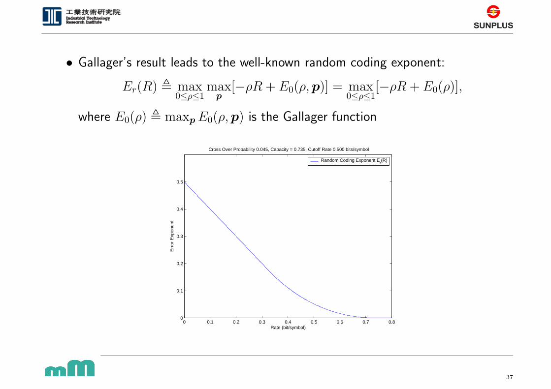
• Gallager’s result leads to the well-known random coding exponent:
Er(R) , max0≤ρ≤1
maxp
[−ρR + E0(ρ, p)] = max0≤ρ≤1
[−ρR + E0(ρ)],
where E0(ρ) , maxp E0(ρ, p) is the Gallager function
0 0.1 0.2 0.3 0.4 0.5 0.6 0.7 0.80
0.1
0.2
0.3
0.4
0.5
Rate (bit/symbol)
Err
or E
xpon
ent
Cross Over Probability 0.045, Capacity = 0.735, Cutoff Rate 0.500 bits/symbol
Random Coding Exponent Er(R)
37
Page 38
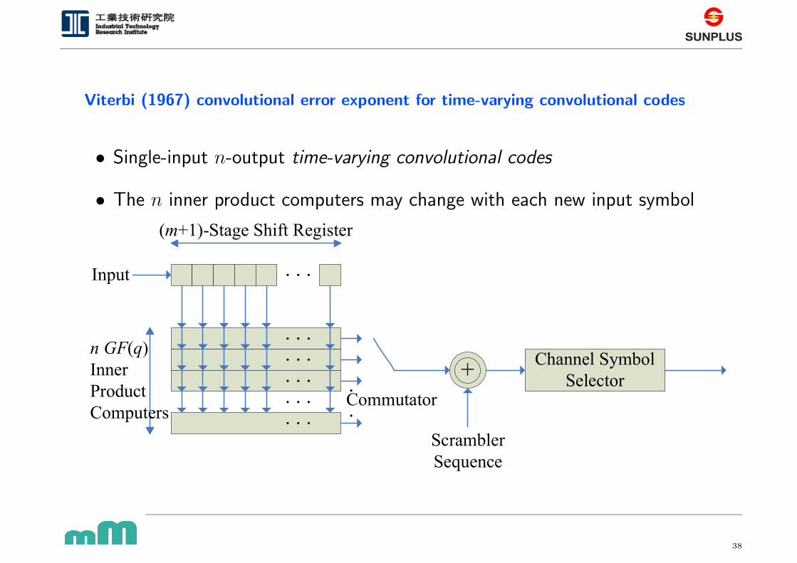
Viterbi (1967) convolutional error exponent for time-varying convolutional codes
• Single-input n-output time-varying convolutional codes
• The n inner product computers may change with each new input symbol
38
Page 39
• Viterbi showed that the ML decoding error Pe,c for time-varying convolutional
codes can be upper-bounded by:
Pe,c ≤1
1 − 2−λ/Rexp[−n(m + 1)E0(ρ)] (2)
for all 0 ≤ ρ ≤ 1, where R , log(2)/n is the code rate in unit of nats per
symbol, and λ , E0(ρ) − ρR is a constant independent of n(m + 1)
• λ is required to be positive
• For symmetric channels, E0(ρ) is an increasing and concave function in ρ
with E0(0) = 0; therefore, Ec(R) can be reduced to:
Ec(R) , max{ρ∈[0,1] : E0(ρ)>ρR}
E0(ρ) =
R0, if 0 ≤ R < R0;
E0(ρ∗), if R0 ≤ R < C;
0, if R ≥ C,
(3)
39
Page 40
where R0 = E0(1) is the cutoff rate, C = E ′0(0) is the channel capacity, and
ρ∗ = ρ∗(R) is the unique solution of E0(ρ) = ρR. It is also shown in the
same work that Ec(R) is a tight exponent for R ≥ R0
0 0.1 0.2 0.3 0.4 0.5 0.6 0.7 0.80
0.1
0.2
0.3
0.4
0.5
Rate (bit/symbol)
Err
or E
xpon
ent
Cross Over Probability 0.045, Capacity = 0.735, Cutoff Rate 0.500 bits/symbol
Convolutional Code Exponent Ec(R)
Random Coding Exponent Er(R)
40
Page 41
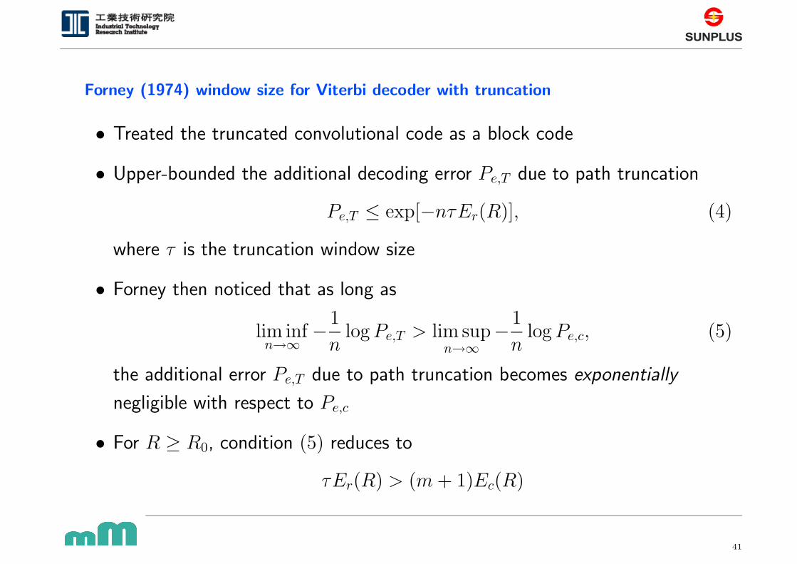
Forney (1974) window size for Viterbi decoder with truncation
• Treated the truncated convolutional code as a block code
• Upper-bounded the additional decoding error Pe,T due to path truncation
Pe,T ≤ exp[−nτEr(R)], (4)
where τ is the truncation window size
• Forney then noticed that as long as
lim infn→∞
−1
nlog Pe,T > lim sup
n→∞−1
nlog Pe,c, (5)
the additional error Pe,T due to path truncation becomes exponentially
negligible with respect to Pe,c
• For R ≥ R0, condition (5) reduces to
τEr(R) > (m + 1)Ec(R)
41
Page 42
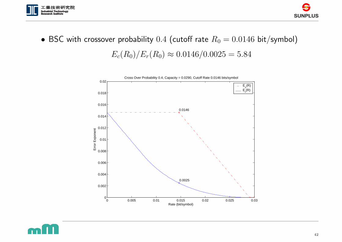
• BSC with crossover probability 0.4 (cutoff rate R0 = 0.0146 bit/symbol)
Ec(R0)/Er(R0) ≈ 0.0146/0.0025 = 5.84
0 0.005 0.01 0.015 0.02 0.025 0.030
0.002
0.004
0.006
0.008
0.01
0.012
0.014
0.016
0.018
0.02
Rate (bit/symbol)
Err
or E
xpon
ent
Cross Over Probability 0.4, Capacity = 0.0290, Cutoff Rate 0.0146 bits/symbol
Ec(R)
Er(R)
0.0146
0.0025
42
Page 43
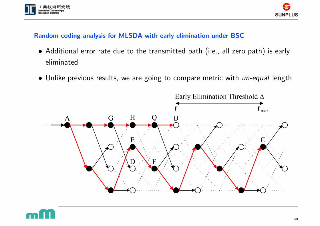
Random coding analysis for MLSDA with early elimination under BSC
• Additional error rate due to the transmitted path (i.e., all zero path) is early
eliminated
• Unlike previous results, we are going to compare metric with un-equal length
43
Page 44
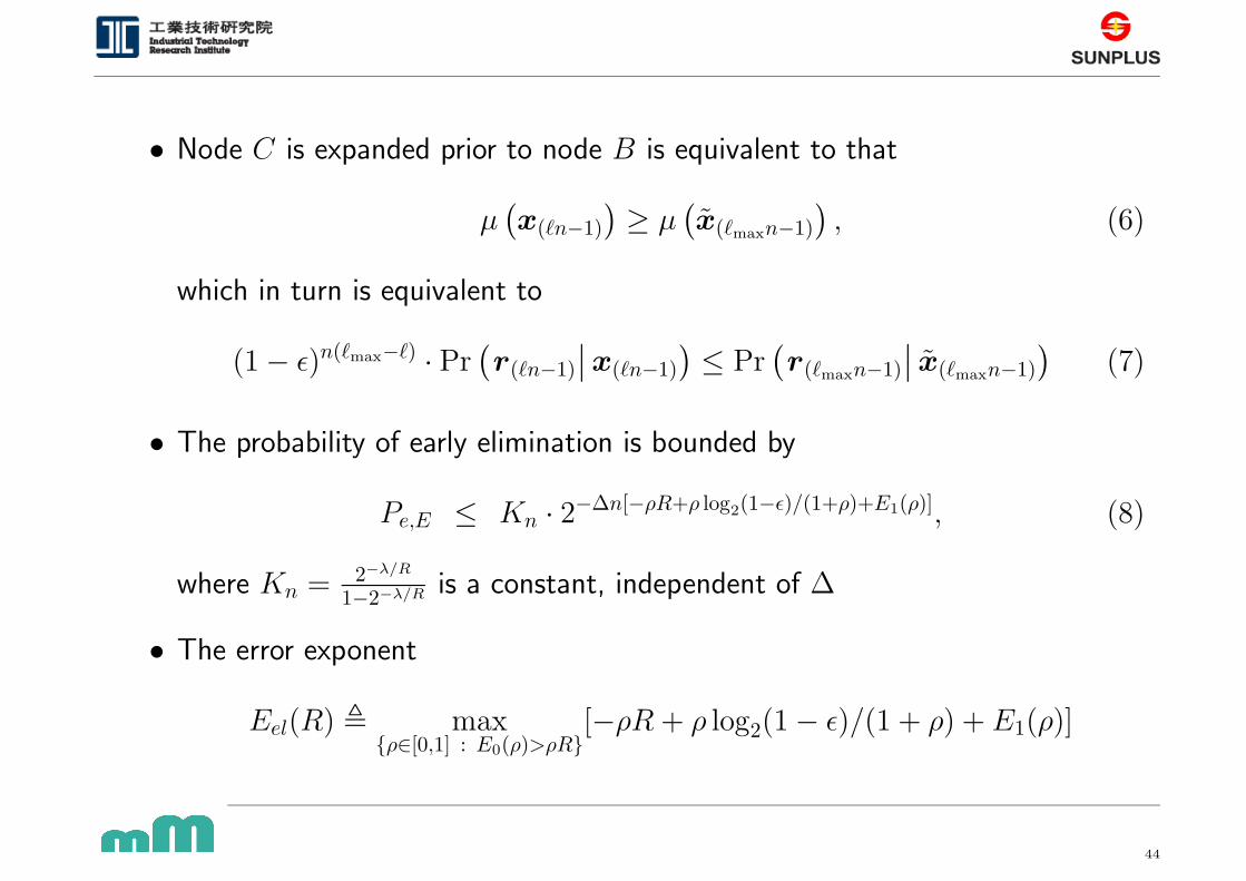
• Node C is expanded prior to node B is equivalent to that
µ(
x(`n−1)
)
≥ µ(
x(`maxn−1)
)
, (6)
which in turn is equivalent to
(1 − ε)n(`max−`) · Pr(
r(`n−1)
∣
∣x(`n−1)
)
≤ Pr(
r(`maxn−1)
∣
∣ x(`maxn−1)
)
(7)
• The probability of early elimination is bounded by
Pe,E ≤ Kn · 2−∆n[−ρR+ρ log2(1−ε)/(1+ρ)+E1(ρ)], (8)
where Kn = 2−λ/R
1−2−λ/R is a constant, independent of ∆
• The error exponent
Eel(R) , max{ρ∈[0,1] : E0(ρ)>ρR}
[−ρR + ρ log2(1 − ε)/(1 + ρ) + E1(ρ)]
44
Page 45
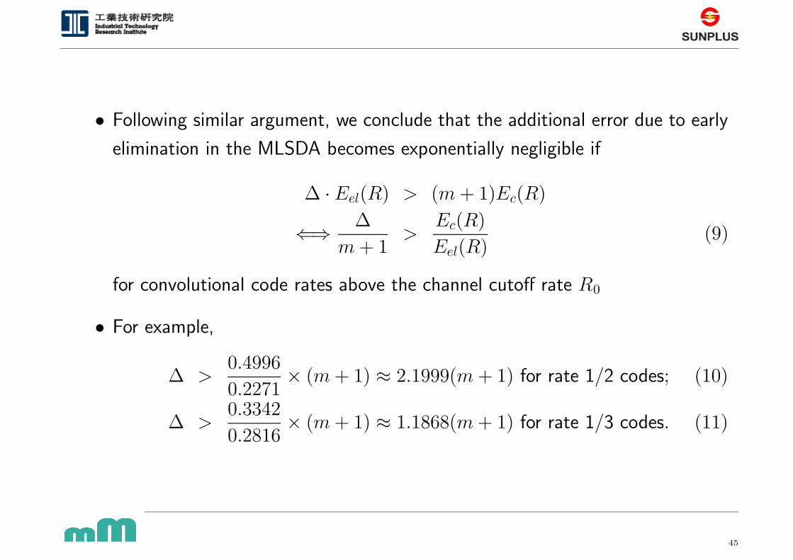
• Following similar argument, we conclude that the additional error due to early
elimination in the MLSDA becomes exponentially negligible if
∆ · Eel(R) > (m + 1)Ec(R)
⇐⇒ ∆
m + 1>
Ec(R)
Eel(R)(9)
for convolutional code rates above the channel cutoff rate R0
• For example,
∆ >0.4996
0.2271× (m + 1) ≈ 2.1999(m + 1) for rate 1/2 codes; (10)
∆ >0.3342
0.2816× (m + 1) ≈ 1.1868(m + 1) for rate 1/3 codes. (11)
45
Page 46
BSC with crossover probability 0.045
0 0.1 0.2 0.3 0.4 0.5 0.6 0.7 0.8 0.9 10
0.1
0.2
0.3
0.4
0.5
0.6
0.7
0.8
0.9
1
Rate (in bit/symbol)
Err
or E
xpon
ent
Cross Over Probability 0.045, Cutoff Rate 0.5 bit/symbol
Random Convolutional Code Ec(R)
MLSDA Early Elimination Eel
(R)
46
Page 47
BSC with crossover probability 0.095
0 0.1 0.2 0.3 0.4 0.5 0.6 0.70
0.1
0.2
0.3
0.4
0.5
0.6
0.7
Rate (in bit/symbol)
Err
or E
xpon
ent
Cross Over Probability 0.095, Cutoff Rate 0.334 bit/symbol
Random Convolutional Code Ec(R)
MLSDA Early Elimination Eel
(R)
47
Page 48
Simulation results for (2,1,12) codes under BSC (∆ > 2.2 × 13 = 28.6)
1 1.5 2 2.5 3 3.5 4 4.5 510
−5
10−4
10−3
10−2
10−1
100
Eb / N
0
Bit
Err
or R
ate
∆=26∆=29ML
48
Page 49
Simulation results for (3,1,8) codes under BSC (∆ > 1.2 × 9 = 10.8)
2 2.5 3 3.5 4 4.5 5 5.5
10−4
10−3
10−2
10−1
Eb / N
0
Bit
Err
or R
ate
MLSDA (∆= 9)MLSDA (∆= 11)ML
49
Page 50
Chapter 5 :
Performance Analysis to a Specific Encoder underAWGN channel
50
Page 51
Main idea of this chapter
• Find the BLER of ML decoder
• Analyze the additional BLER (as a function of early elimination threshold ∆)
due to the introduce of early elimination in MLSDA
• Find the smallest value of ∆ such that the additional BLER is small
compared with the BLER of ML decoder
51
Page 52
Block error rate upper bound for finite-length convolutional codes with ML decoder
• The weight enumerator function (WEF) A(x) is defined as
A(x) =∞∑
d=dfree
Adxd,
where dfree is the free distance and Ad denote the number of codewords with
weight d
• For example, the WEF for (2,1,6) convolutional code with generator
polynomial [554,744] (in oct) is
A(x) = 11x10 + 38x12 + 193x14 + 1331x16 + 7275x18 + 40406x20 + · · ·
52
Page 53
• Define the first event error is made at time unit t if the correct path is
eliminated (in Viterbi decoder) for the first time at time unit t in favor of a
competitor path
• For infinite-length convolutional code under binary-input AWGN channel, the
first event error probability Pev can be obtained
Pev ≤∞∑
d=dfree
AdQ
(
√
2dREb
N0
)
(12)
• For finite-length convolutional code, the above upper bound is still valid
• With finite information length L, we obtain the BLER upper bound PB as
PB = L · Pev (13)
53
Page 54
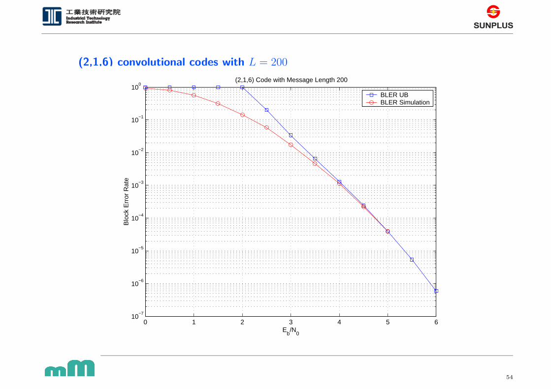
(2,1,6) convolutional codes with L = 200
0 1 2 3 4 5 610
−7
10−6
10−5
10−4
10−3
10−2
10−1
100
Eb/N
0
Blo
ck E
rror
Rat
e
(2,1,6) Code with Message Length 200
BLER UB BLER Simulation
54
Page 55
(2,1,10) convolutional codes with L = 200
0 0.5 1 1.5 2 2.5 3 3.5 4 4.510
−6
10−5
10−4
10−3
10−2
10−1
100
Eb/N
0
Err
or R
ate
(2,1,10) Code with Message Length 200
BLER UB = 200 * NER UBBLER Simulation
55
Page 56
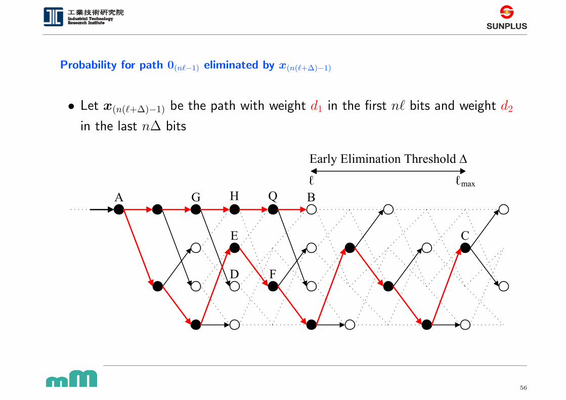
Probability for path 0(n`−1) eliminated by x(n(`+∆)−1)
• Let x(n(`+∆)−1) be the path with weight d1 in the first n` bits and weight d2
in the last n∆ bits
�� � �
� � � � � � � � � � � � � � � � � � � � �
�
�
�
�
� �
�
�
�
�
56
Page 57
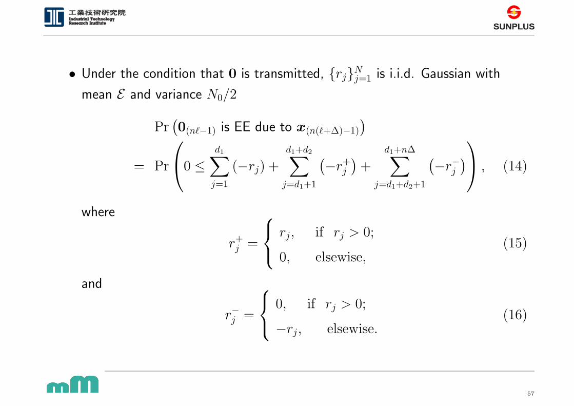
• Under the condition that 0 is transmitted, {rj}Nj=1 is i.i.d. Gaussian with
mean E and variance N0/2
Pr(
0(n`−1) is EE due to x(n(`+∆)−1)
)
= Pr
0 ≤d1∑
j=1
(−rj) +
d1+d2∑
j=d1+1
(
−r+j
)
+
d1+n∆∑
j=d1+d2+1
(
−r−j)
, (14)
where
r+j =
rj, if rj > 0;
0, elsewise,(15)
and
r−j =
0, if rj > 0;
−rj, elsewise.(16)
57
Page 58
Moment generating bound
• The moment generating functions M(t), M+(t), and M−(t) are as follows:
M(t) = exp
(
N0t2
4− Et
)
M+(t) = Q
(
E√
N0/2
)
+ exp
(
N0t2
4− Et
)
Q
(
N0t − 2E√2N0
)
M−(t) = 1 − Q
(
E√
N0/2
)
+ exp
(
N0t2
4+ Et
)
Q
(
N0t + 2E√2N0
)
• The probability is therefore upper bound by the moment generating bound
Pr
0 ≤d1∑
j=1
(−rj) +
d1+d2∑
j=d1+1
(
−r+j
)
+
d1+n∆∑
j=d1+d2+1
(
−r−j)
≤ [M(t)]d1 · [M+(t)]d2 · [M−(t)]n∆−d2 , for t > 0. (17)
58
Page 59
Weight distribution function
• Let P `+∆ be the set of paths of length n(` + ∆) that diverge from 0(n`−1) at
level 0 and never return to all zero state
• Define the weight distribution function for all paths in P `+∆ by
W (`, ∆) =∑
d1,d2
Ad1,d2(`, ∆) · wd1
1 · wd2
2 , (18)
where Ad1,d2(`, ∆) is the number of paths with weight d1 in the first n` bits
and weight d2 in the last n∆ bits.
• For example, for (2,1,6) convolutional code with g(x) = [554, 744],
W (2, 3) = 2w31w2 + 3w3
1w22 + 6w3
1w32 + 4w3
1w42 + w3
1w62.
• Therefore, for each early elimination threshold ∆
Pr(
0(n`−1) is EE)
≤∑
d1,d2
Ad1,d2(`, ∆) · min
t>0
[
M(t)d1 · M+(t)d2 · M−(t)n∆−d2]
59
Page 60
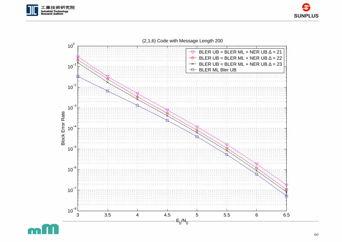
3 3.5 4 4.5 5 5.5 6 6.510
−8
10−7
10−6
10−5
10−4
10−3
10−2
10−1
100
Eb/N
0
Blo
ck E
rror
Rat
e
(2,1,6) Code with Message Length 200
BLER UB = BLER ML + NER UB ∆ = 21BLER UB = BLER ML + NER UB ∆ = 22BLER UB = BLER ML + NER UB ∆ = 23BLER ML Bler UB
60
Page 61
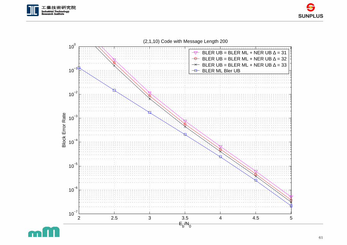
2 2.5 3 3.5 4 4.5 510
−7
10−6
10−5
10−4
10−3
10−2
10−1
100
Eb/N
0
Blo
ck E
rror
Rat
e
(2,1,10) Code with Message Length 200
BLER UB = BLER ML + NER UB ∆ = 31BLER UB = BLER ML + NER UB ∆ = 32BLER UB = BLER ML + NER UB ∆ = 33BLER ML Bler UB
61
Page 62
2 2.5 3 3.5 4 4.5 510
−5
10−4
10−3
10−2
10−1
100
Eb / N
0
Blo
ck E
rror
Rat
e
(2,1,6), Message Length 200
∆=16∆=18∆=20ML
62
Page 63
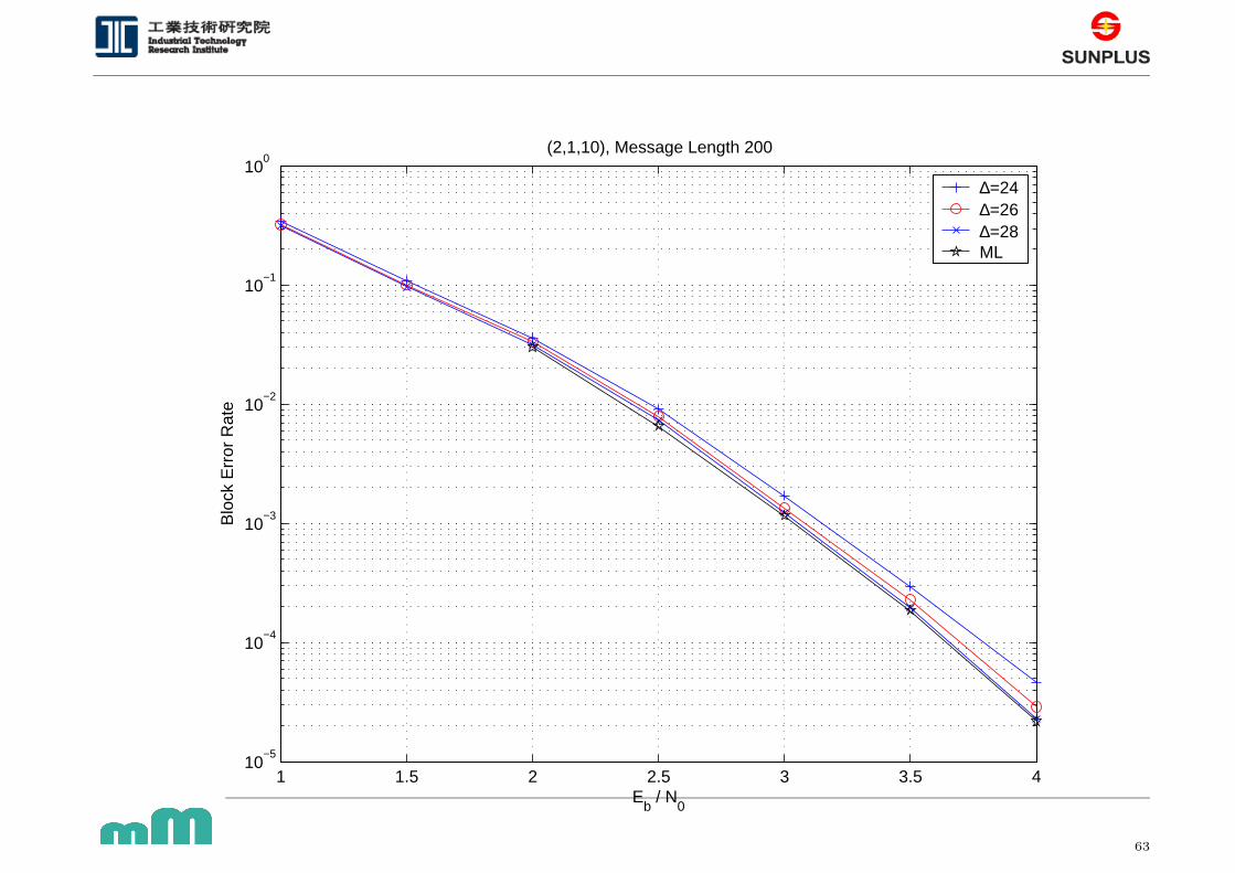
1 1.5 2 2.5 3 3.5 410
−5
10−4
10−3
10−2
10−1
100
Eb / N
0
Blo
ck E
rror
Rat
e
(2,1,10), Message Length 200
∆=24∆=26∆=28ML
63
Page 64
Table 1: Suggested ∆ values for rate one-half convolutional codes
Memory Order m 6 8 10 12 14 16
Generator Polynomial 554 561 4672 42554 56721 716502
744 753 7542 77304 61713 514576
Minimum Distance dmin 10 12 14 16 18 20
Sufficiently Large ∆ by UB 23 29 33 38 42 46
Sufficiently Large ∆ by Simulation 20 24 28 32 36 40
64
Page 65
Chapter 6 :
Complexity Analysis Based on Large DeviationsTechnique & Berry-Esseen Theorem
65
Page 66
Berry-Esseen theorem
• The large deviations technique is generally applied to compute the exponent
of an exponentially decaying probability mass.
• The Berry-Esseen inequality to evaluate the subexponential detail of the
concerned probability to obtain a better complexity upper bound.
• Let {Xi}ni=1 be independent zero-mean random variables. For every a ∈ <,
∣
∣
∣
∣
Pr
{
1
sn(X1 + · · · + Xn) ≤ a
}
− Φ(a)
∣
∣
∣
∣
≤ Crn
s3n
, (19)
where Φ(·) represents the unit Gaussian cdf, s2n and rn are, respectively, the
sums of the marginal variances and the marginal absolute third moments, and
the Berry-Esseen coefficient, C, is an absolute constant.
66
Page 67
Upper bound for sum of i.i.d. non-Gaussian rv
Lemma 1 (main idea) Let Yn =∑n
i=1 Xi be the sum of i.i.d. random variables.
Then, for every θ < 0,
Pr {Yn ≤ −nα} ≤ An(θ, α)eθαnMn(θ),
where M(θ) , E[eθX1] and
An(θ, α) = min{Bn(θ, α), 1} ≈ min{2C ρ(θ)
σ3(θ)√
n, 1}.
• Note: Chernoff bound eθαnMn(θ)
67
Page 68
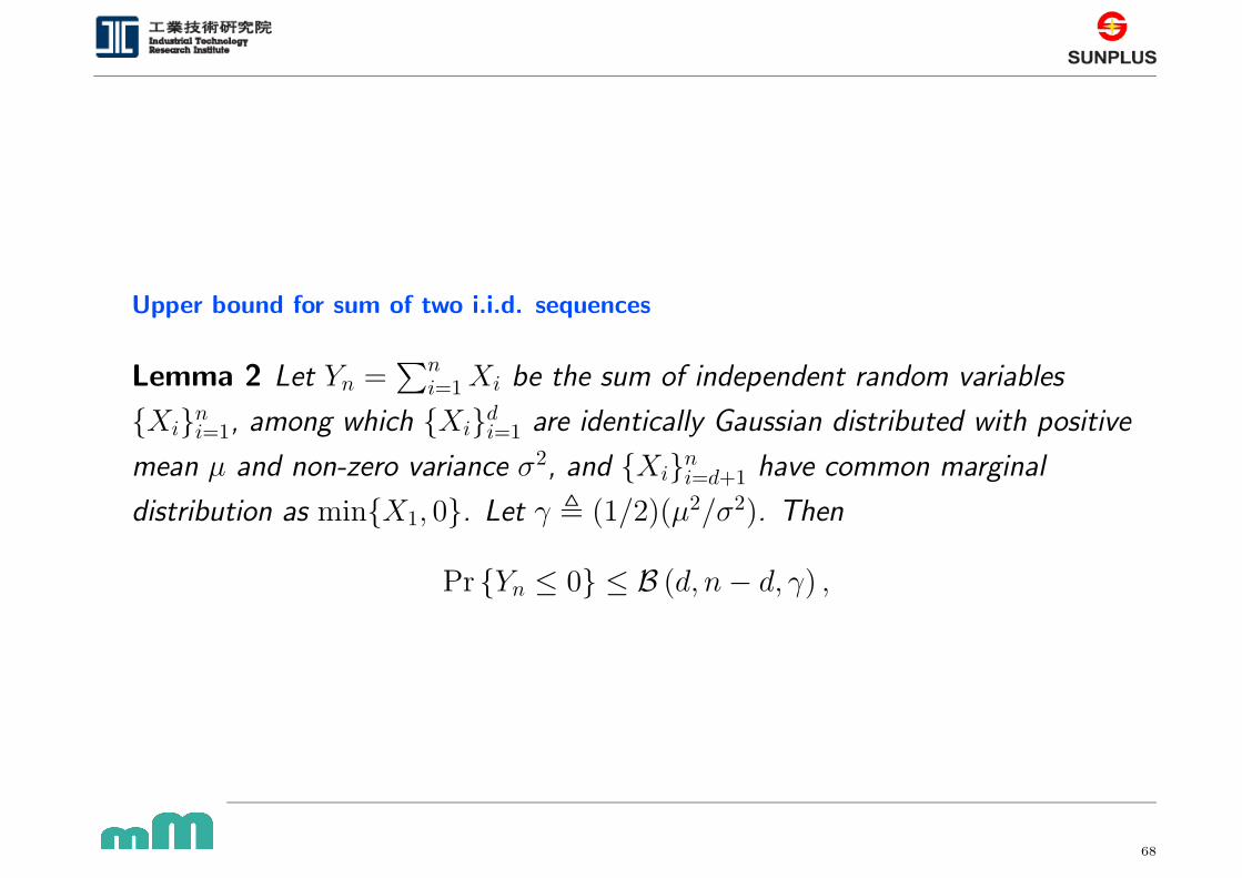
Upper bound for sum of two i.i.d. sequences
Lemma 2 Let Yn =∑n
i=1 Xi be the sum of independent random variables
{Xi}ni=1, among which {Xi}d
i=1 are identically Gaussian distributed with positive
mean µ and non-zero variance σ2, and {Xi}ni=d+1 have common marginal
distribution as min{X1, 0}. Let γ , (1/2)(µ2/σ2). Then
Pr {Yn ≤ 0} ≤ B (d, n − d, γ) ,
68
Page 69
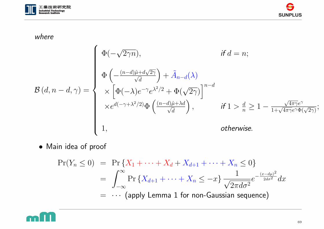
where
B (d, n − d, γ) =
Φ(−√2γn), if d = n;
Φ(
− (n−d)µ+d√
2γ√d
)
+ An−d(λ)
×[
Φ(−λ)e−γeλ2/2 + Φ(√
2γ)]n−d
×ed(−γ+λ2/2)Φ(
(n−d)µ+λd√d
)
, if 1 > dn ≥ 1 −
√4πγeγ
1+√
4πγeγΦ(√
2γ);
1, otherwise.
• Main idea of proof
Pr(Yn ≤ 0) = Pr {X1 + · · · + Xd + Xd+1 + · · · + Xn ≤ 0}
=
∫ ∞
−∞Pr {Xd+1 + · · · + Xn ≤ −x} 1√
2πdσ2e−
(x−dµ)2
2dσ2 dx
= · · · (apply Lemma 1 for non-Gaussian sequence)
69
Page 70
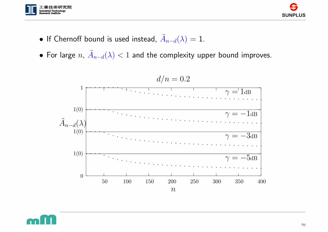
• If Chernoff bound is used instead, An−d(λ) = 1.
• For large n, An−d(λ) < 1 and the complexity upper bound improves.
0
1(0)
1(0)
1(0)
1
50 100 150 200 250 300 350 400
n
d/n = 0.2
γ = −5dB
γ = −3dB
γ = −1dB
γ = 1dB
An−d(λ)
70
Page 71
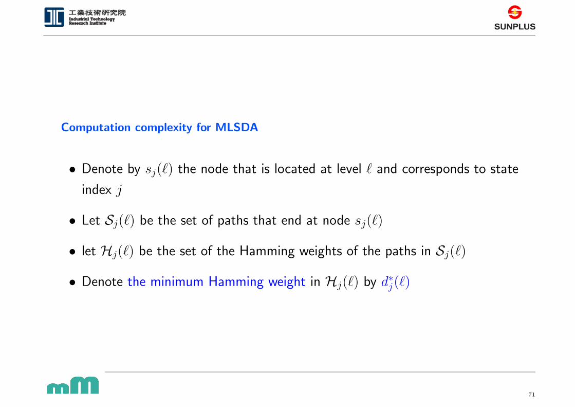
Computation complexity for MLSDA
• Denote by sj(`) the node that is located at level ` and corresponds to state
index j
• Let Sj(`) be the set of paths that end at node sj(`)
• let Hj(`) be the set of the Hamming weights of the paths in Sj(`)
• Denote the minimum Hamming weight in Hj(`) by d∗j(`)
71
Page 72
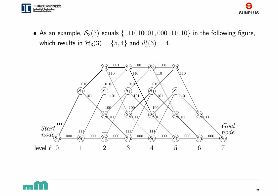
• As an example, S3(3) equals {111010001, 000111010} in the following figure,
which results in H3(3) = {5, 4} and d∗3(3) = 4.
n n n n n n n ns0 s0 s0 s0 s0 s0 s0 s0
n n n n ns1 s1 s1 s1 s1
n n n n ns2 s2 s2 s2 s2
n n n ns3 s3 s3 s3
���������
���������
���������
���������
���������
��
��
��
��
��
��
��
��
@@
@@
@@
@@
@@
@@
@@
@@
@@
@@
@@
@@
@@
@@
@@
@@
@@
@@
@@
@@
AAAAAAAAA
AAAAAAAAA
AAAAAAAAA
AAAAAAAAA�
��
�
��
��
��
��
Startnode
Goalnode
level ` 0 1 2 3 4 5 6 7
000 000 000 000 000 000 000
111
111 111 111 111
101 101 101 101 101
010 010 010 010
001 001 001
110 110 110 110
100 100 100
011 011 011 011 011
���������
��
�� A
AAAAAAAA �
��
� @@
@@
@@
@@
72
Page 73
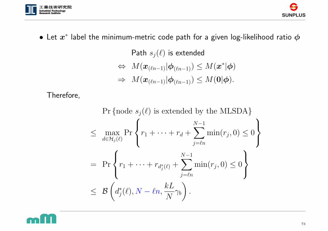
• Let x∗ label the minimum-metric code path for a given log-likelihood ratio φ
Path sj(`) is extended
⇔ M(x(`n−1)|φ(`n−1)) ≤ M(x∗|φ)
⇒ M(x(`n−1)|φ(`n−1)) ≤ M(0|φ).
Therefore,
Pr {node sj(`) is extended by the MLSDA}
≤ maxd∈Hj(`)
Pr
r1 + · · · + rd +N−1∑
j=`n
min(rj, 0) ≤ 0
= Pr
r1 + · · · + rd∗j (`)+
N−1∑
j=`n
min(rj, 0) ≤ 0
≤ B(
d∗j(`), N − `n,kL
Nγb
)
.
73
Page 74
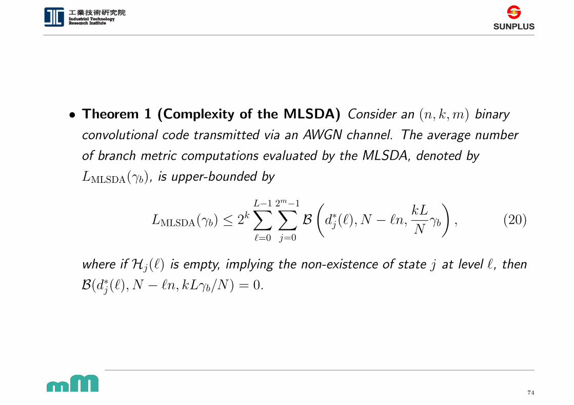
• Theorem 1 (Complexity of the MLSDA) Consider an (n, k, m) binary
convolutional code transmitted via an AWGN channel. The average number
of branch metric computations evaluated by the MLSDA, denoted by
LMLSDA(γb), is upper-bounded by
LMLSDA(γb) ≤ 2kL−1∑
`=0
2m−1∑
j=0
B(
d∗j(`), N − `n,kL
Nγb
)
, (20)
where if Hj(`) is empty, implying the non-existence of state j at level `, then
B(d∗j(`), N − `n, kLγb/N) = 0.
74
Page 75
Computation complexity for MLSDA with early elimination
• MLSDA with early elimination, in the “normal case”
Pr {node sj(`) is extended by the MLSDA with EE in the normal case}
≤ B(
d∗j(`), ∆n,kL
Nγb
)
.
(( ) 1)o
nC x +∆ −=�
( 1)nA x −=� *
(( ) 1)nB x +∆ −=�
(( ) 1)0 nD +∆ −=�
'C
'D
'B
Threshold ∆
O
75
Page 76
• ”Abnormal case”: The first expanded path x◦((`+∆)n−1) > 0((`+∆)n−1)
– x◦((`+∆)n−1) may not be the best path at the same level
– abnormal case ⇒ early elimination of 0((`+∆)n−1)
– probability can be upper bounded by the BLER of MLSDA with EE
• Overall complexity upper bound
LEE(γb) ≤ 2kL−1∑
`=0
2m−1∑
j=0
[
PEE(γb, ∆) + B(
d∗j(`), ∆n,kL
Nγb
)]
,
= L · 2k+m · PEE(γb, ∆) + 2kL−1∑
`=0
2m−1∑
j=0
B(
d∗j(`), ∆n,kL
Nγb
)
,
where PEE(γb, ∆) denotes the block error rate of MLSDA with early
elimination window ∆ under SNR γb.
76
Page 77
Complexity UB vs simulation result for (2,1,10) code with L = 100
1 2 3 4 5 6 710
0
101
102
103
104
Eb / N
0
Ave
rage
Dec
odin
g C
ompl
exity
Per
Out
put B
it
(2,1,10) Convolutional codes, ∆ = 30
UB MLSDASim MLSDAUB MLSDA with EEUB MLSDA with EE ignoring BLER termSimulation
77
Page 78
Complexity UB vs simulation result for (2,1,10) code with SNR = 3.5 dB
50 100 150 200 250 300 35010
0
101
102
103
104
Message Length
Ave
rage
Dec
odin
g C
ompl
exity
Per
Info
rmat
ion
Bit
UB MLSDASim MLSDAUB MLSDA with EESim MLSDA with EE
78
Page 79
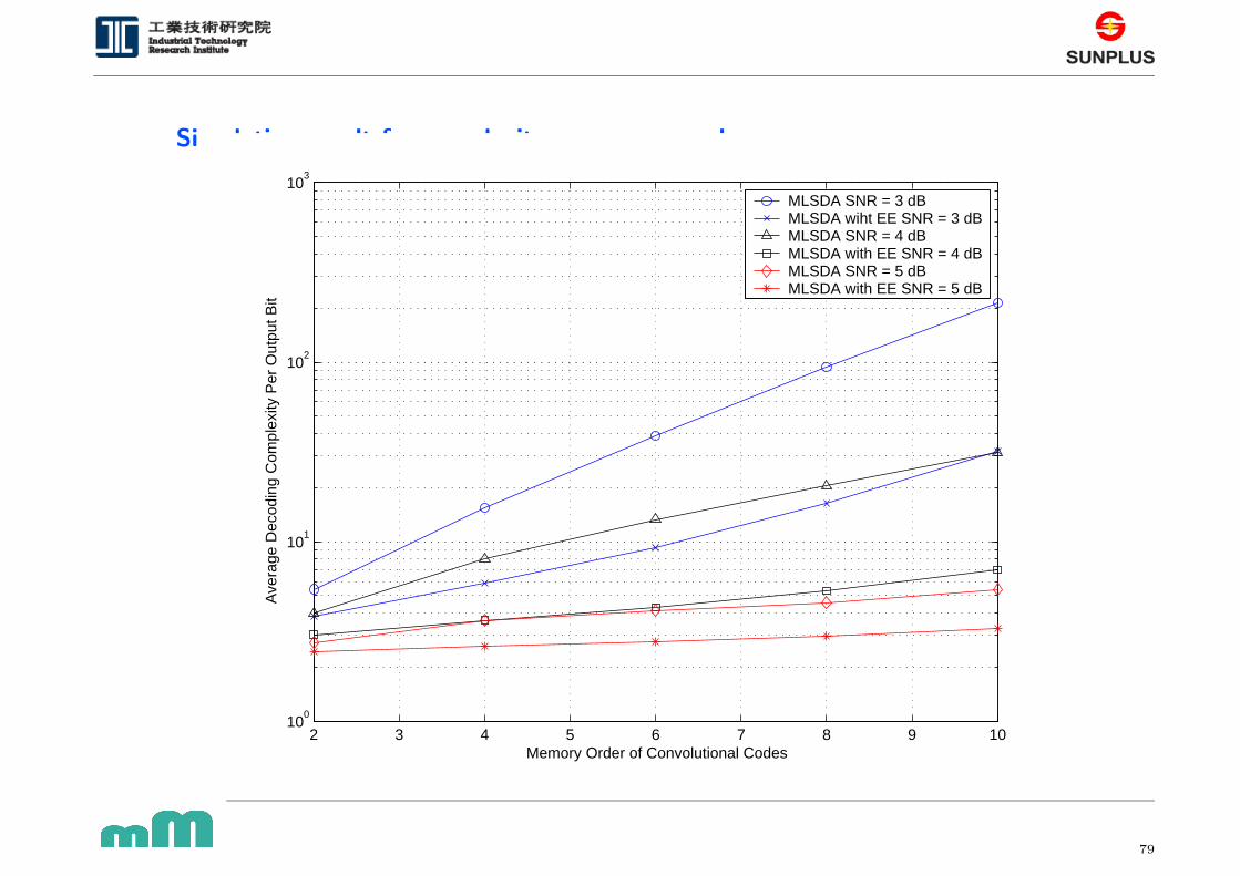
Simulation result for complexity vs memory order
2 3 4 5 6 7 8 9 1010
0
101
102
103
Memory Order of Convolutional Codes
Ave
rage
Dec
odin
g C
ompl
exity
Per
Out
put B
it
MLSDA SNR = 3 dBMLSDA wiht EE SNR = 3 dBMLSDA SNR = 4 dBMLSDA with EE SNR = 4 dBMLSDA SNR = 5 dBMLSDA with EE SNR = 5 dB
79
Page 80
Chapter 7 :
Concluding Remarks
80
Page 81
• Early elimination is proposed to reduce decoding complexity of MLSDA
• Performance analyses suggest the sufficient threshold value for negligible
performance degradation
• Complexity analysis confirms the large complexity reduction compared with
the original MLSDA
• The performance and complexity analytic results are further justified by
simulation results
81
Page 82
Acknowledgement
• Industrial Technology Research Institute (ITRI)
• Sunplus Technology Co., Ltd. (Sunplus)
• Sunplus mMobile Inc. (SunplusMM)
82
Page 83
Thank You for Your Attention!
Questions & Answers
83