Necessary and Sufficient Informativity Conditions for ...

Necessary and Sufficient Informativity Conditions for Robust Network

Reconstruction Using Dynamical Structure Functions

Vasu Chetty

A thesis submitted to the faculty ofBrigham Young University

in partial fulfillment of the requirements for the degree of

Master of Science

Sean Warnick, ChairJulianne GroseDaniel Zappala

Department of Computer Science

Brigham Young University

December 2012

Copyright c© 2012 Vasu Chetty

All Rights Reserved

ABSTRACT

Necessary and Sufficient Informativity Conditions for Robust NetworkReconstruction Using Dynamical Structure Functions

Vasu ChettyDepartment of Computer Science, BYU

Master of Science

Dynamical structure functions were developed as a partial structure representationof linear time-invariant systems to be used in the reconstruction of biological networks.Dynamical structure functions contain more information about structure than a system’stransfer function, while requiring less a priori information for reconstruction than the completecomputational structure associated with the state space realization. Early sufficient conditionsfor network reconstruction with dynamical structure functions severely restricted the possibleapplications of the reconstruction process to networks where each input independently controlsa measured state.

The first contribution of this thesis is to extend the previously established sufficientconditions to incorporate both necessary and sufficient conditions for reconstruction. Thesenew conditions allow for the reconstruction of a larger number of networks, even networkswhere independent control of measured states is not possible.

The second contribution of this thesis is to extend the robust reconstruction algorithmto all reconstructible networks. This extension is important because it allows for thereconstruction of networks from real data, where noise is present in the measurements of thesystem.

The third contribution of this thesis is a Matlab toolbox that implements the robustreconstruction algorithm discussed above. The Matlab toolbox takes in input-output datafrom simulations or real-life perturbation experiments and returns the proposed Booleanstructure of the network.

The final contribution of this thesis is to increase the applicability of dynamicalstructure functions to more than just biological networks by applying our reconstructionmethod to wireless communication networks. The reconstruction of wireless networks producesa dynamic interference map that can be used to improve network performance or interpretchanges of link rates in terms of changes in network structure, enabling novel anomalydetection and security schemes.

Keywords: Realization theory, dynamical structure functions, informativity conditions, net-work reconstruction, network inference, system identification, dynamic interference maps,wireless networks, PAS Kinase pathway, chemical reaction networks, partial structure repre-sentation, linear time-invariant systems

ACKNOWLEDGMENTS

I would like to thank my wonderful wife, Leticia Chetty, for all her help and support.

I would also like to thank all my colleagues in the IDeA Labs at Brigham Young University,

especially Julius Adebayo, Anurag Rai, and Devon Harbaugh for all their ideas and contri-

butions to this thesis. Finally, I would like to thank my thesis committee, my advisor Sean

Warnick, Julianne Grose, and Daniel Zappala, and all our other contributors with our work

in Dynamical Structure Functions, especially Ye Yuan and Jorge Goncalves.

Table of Contents

List of Figures vii

List of Tables ix

1 Introduction 1

1.1 Modeling Wireless Networks . . . . . . . . . . . . . . . . . . . . . . . . . . . 2

1.2 Modeling Biological Networks . . . . . . . . . . . . . . . . . . . . . . . . . . 5

1.2.1 The Hill Equation . . . . . . . . . . . . . . . . . . . . . . . . . . . . . 7

1.3 Network Structure Representations . . . . . . . . . . . . . . . . . . . . . . . 9

1.3.1 Complete Computational Structure . . . . . . . . . . . . . . . . . . . 11

1.3.2 Subsystem Structure . . . . . . . . . . . . . . . . . . . . . . . . . . . 13

1.3.3 Signal Structure . . . . . . . . . . . . . . . . . . . . . . . . . . . . . . 14

1.3.4 Network Reconstruction . . . . . . . . . . . . . . . . . . . . . . . . . 15

2 Related Work 18

2.1 Correlation Methods . . . . . . . . . . . . . . . . . . . . . . . . . . . . . . . 18

2.2 Bayesian Networks . . . . . . . . . . . . . . . . . . . . . . . . . . . . . . . . 19

2.3 Dynamic Models . . . . . . . . . . . . . . . . . . . . . . . . . . . . . . . . . 20

2.4 Direction of Research in Systems Biology . . . . . . . . . . . . . . . . . . . . 21

2.5 Interference Maps for Wireless Networks . . . . . . . . . . . . . . . . . . . . 22

3 Foundational Material 24

3.1 Sufficient Informativity Conditions for Network Reconstruction . . . . . . . . 25

iv

3.2 Robust Reconstruction from G . . . . . . . . . . . . . . . . . . . . . . . . . . 26

3.3 Robust Reconstruction from Data . . . . . . . . . . . . . . . . . . . . . . . . 27

3.4 Penalizing Connections using an Information Criterion . . . . . . . . . . . . 28

4 Necessary and Sufficient Informativity Conditions 30

4.1 Necessary and Sufficient Conditions for Network Reconstruction . . . . . . . 30

4.2 Necessary and Sufficient Informativity Conditions Examples . . . . . . . . . 33

5 Robust Network Reconstruction 38

5.1 Robust Reconstruction Problem . . . . . . . . . . . . . . . . . . . . . . . . . 38

5.2 Robust Reconstruction Algorithm . . . . . . . . . . . . . . . . . . . . . . . . 40

5.2.1 Total Least Squares . . . . . . . . . . . . . . . . . . . . . . . . . . . . 41

5.2.2 Penalizing Connections using an Information Criterion . . . . . . . . 42

5.3 Robust Reconstruction Examples . . . . . . . . . . . . . . . . . . . . . . . . 43

5.3.1 Example 1: Diagonal P . . . . . . . . . . . . . . . . . . . . . . . . . . 43

5.3.2 Example 2: Diagonal P with Noise . . . . . . . . . . . . . . . . . . . 45

5.3.3 Example 3: Non-Diagonal P . . . . . . . . . . . . . . . . . . . . . . . 46

5.3.4 Non-Diagonal P with Noise . . . . . . . . . . . . . . . . . . . . . . . 48

6 Matlab Toolbox 50

6.1 List of Functions . . . . . . . . . . . . . . . . . . . . . . . . . . . . . . . . . 50

6.2 Verification of Matlab Toolbox Functions . . . . . . . . . . . . . . . . . . . . 54

7 Validation and Analysis of Reconstruction Technique 65

7.1 Comparison of VICc to Distance, α . . . . . . . . . . . . . . . . . . . . . . . 65

7.2 Accuracy of Robust Reconstruction . . . . . . . . . . . . . . . . . . . . . . . 66

7.3 Specificity and Sensitivity of Robust Reconstruction Technique . . . . . . . . 68

8 Applications to Biological Networks 70

8.1 PAS Kinase Pathway . . . . . . . . . . . . . . . . . . . . . . . . . . . . . . . 70

v

8.2 Reconstruction for PAS Kinase Pathway . . . . . . . . . . . . . . . . . . . . 73

8.3 Simulation of the PAS Kinase Pathway . . . . . . . . . . . . . . . . . . . . . 75

9 Applications to Wireless Networks 77

9.1 Reconstruction Without Transitory Interference . . . . . . . . . . . . . . . . 77

9.2 Reconstruction With Transitory Interference . . . . . . . . . . . . . . . . . . 81

10 Overview of Contributions and Future Work with Dynamical Structure

Functions 84

10.1 Major Contribution 1: Necessary and Sufficient Identifiability Conditions . . 84

10.2 Major Contribution 2: Robust Reconstruction Algorithm for Networks with

Non-Diagonal P . . . . . . . . . . . . . . . . . . . . . . . . . . . . . . . . . . 85

10.3 Major Contribution 3: Matlab Toolbox for Robust Network Reconstruction . 85

10.4 Major Contribution 4: Applying Dynamical Structure Functions to Wireless

Networks . . . . . . . . . . . . . . . . . . . . . . . . . . . . . . . . . . . . . . 86

10.5 Future Work: Theoretical Results . . . . . . . . . . . . . . . . . . . . . . . . 86

10.6 Future Work: Applications . . . . . . . . . . . . . . . . . . . . . . . . . . . . 87

11 References 89

12 Appendix 96

vi

List of Figures

1.1 (a) Stable limit cycle, (b) Unstable limit cycle . . . . . . . . . . . . . . . . . 11

1.2 Complete Computational Structure . . . . . . . . . . . . . . . . . . . . . . . 12

1.3 Subsystem Structure . . . . . . . . . . . . . . . . . . . . . . . . . . . . . . . 13

1.4 Signal Structure . . . . . . . . . . . . . . . . . . . . . . . . . . . . . . . . . . 15

1.5 The Reconstruction Process . . . . . . . . . . . . . . . . . . . . . . . . . . . 16

4.1 Simple Two-Node Network with Non-Diagonal P . . . . . . . . . . . . . . . 37

5.1 Additive uncertainty on P . . . . . . . . . . . . . . . . . . . . . . . . . . . . 38

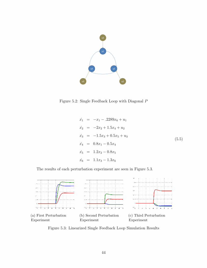
5.2 Single Feedback Loop with Diagonal P . . . . . . . . . . . . . . . . . . . . . 44

5.3 Linearized Single Feedback Loop Simulation Results . . . . . . . . . . . . . . 44

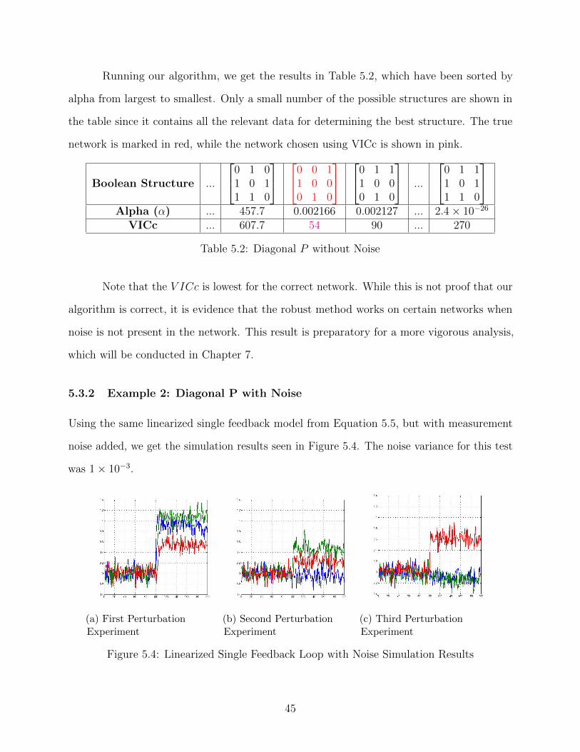
5.4 Linearized Single Feedback Loop with Noise Simulation Results . . . . . . . 45

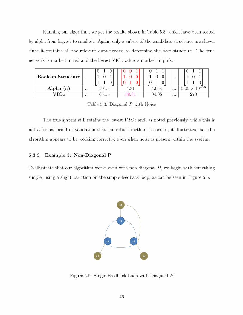
5.5 Single Feedback Loop with Diagonal P . . . . . . . . . . . . . . . . . . . . . 46

5.6 Linearized Single Feedback Loop with Non-Diagonal P Simulation Results . 47

5.7 Linearized Single Feedback Loop with Non-Diagonal P and Noise Simulation

Results . . . . . . . . . . . . . . . . . . . . . . . . . . . . . . . . . . . . . . . 48

6.1 Hierarchy of Function Calls in Matlab Toolbox . . . . . . . . . . . . . . . . . 54

7.1 Comparing VICc to α Values . . . . . . . . . . . . . . . . . . . . . . . . . . 66

7.2 Closer Inspection of VICc and α Comparison . . . . . . . . . . . . . . . . . . 67

7.3 Accuracy of Reconstruction with increasing Noise Variance . . . . . . . . . . 67

7.4 Accuracy of Reconstruction using Noise Averaging . . . . . . . . . . . . . . . 68

vii

8.1 PAS Kinase Pathway with H1 and H2 representing networks of unobserved

nodes . . . . . . . . . . . . . . . . . . . . . . . . . . . . . . . . . . . . . . . . 71

8.2 Experimental setup for PAS Kinase Pathway . . . . . . . . . . . . . . . . . . 72

9.1 Example wireless network, with transitory devices shown in red, along with

corresponding contention graph. . . . . . . . . . . . . . . . . . . . . . . . . . 78

9.2 Structure of the DSF before and after intrusion. . . . . . . . . . . . . . . . . 79

9.3 Perturbation Experiments for Wireless Network without Transitory Interference 80

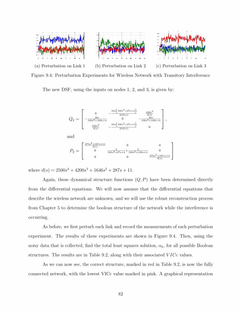
9.4 Perturbation Experiments for Wireless Network with Transitory Interference 82

viii

List of Tables

5.1 Total Least Squares Algorithm . . . . . . . . . . . . . . . . . . . . . . . . . . 42

5.2 Diagonal P without Noise . . . . . . . . . . . . . . . . . . . . . . . . . . . . 45

5.3 Diagonal P with Noise . . . . . . . . . . . . . . . . . . . . . . . . . . . . . . 46

5.4 Non-Diagonal P without Noise . . . . . . . . . . . . . . . . . . . . . . . . . 47

5.5 Non-Diagonal P with Noise . . . . . . . . . . . . . . . . . . . . . . . . . . . 48

6.1 Functions created for Matlab Toolbox . . . . . . . . . . . . . . . . . . . . . . 53

6.2 Test Cases for function createDiag . . . . . . . . . . . . . . . . . . . . . . . . 54

6.3 Test Cases for function findT . . . . . . . . . . . . . . . . . . . . . . . . . . 57

6.4 Test Cases for function findCombs . . . . . . . . . . . . . . . . . . . . . . . . 58

6.5 Test Cases for function getAlpha: Finding Points on the Unit Circle . . . . . 59

6.6 Test Cases for function getAlpha: Removing Columns of M . . . . . . . . . 59

6.7 Test Cases for function zTransform . . . . . . . . . . . . . . . . . . . . . . . 60

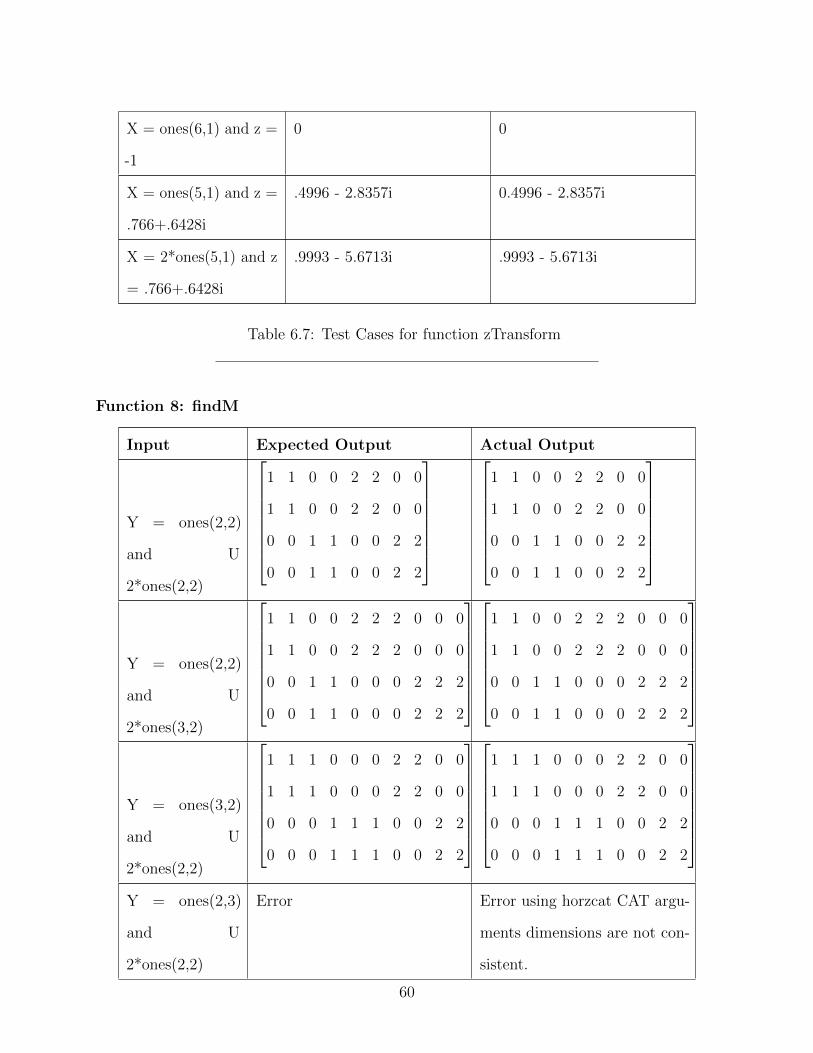
6.8 Test Cases for function findM . . . . . . . . . . . . . . . . . . . . . . . . . . 61

6.9 Test Cases for function vectorize . . . . . . . . . . . . . . . . . . . . . . . . . 61

6.10 Test Cases for function numNonZero . . . . . . . . . . . . . . . . . . . . . . 62

6.11 Test Cases for function vicc . . . . . . . . . . . . . . . . . . . . . . . . . . . 62

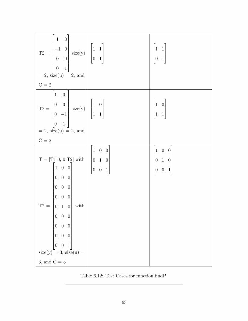
6.12 Test Cases for function findP . . . . . . . . . . . . . . . . . . . . . . . . . . 63

9.1 Reconstruction Without Transient Interference . . . . . . . . . . . . . . . . . 80

9.2 Reconstruction With Transient Interference . . . . . . . . . . . . . . . . . . 83

ix

Chapter 1

Introduction

The problem of network reconstruction, also known as reverse engineering or network

inference, is defined differently for varying applications. However, no matter what the

application, the network reconstruction problem is the attempt to discover the underlying

structure of a particular system, [1].

Network reconstruction in biological systems has been of recent interest in the systems

biology community, [2], [3], [4], [5], [6], [7]. The network reconstruction process has aided

biologists in understanding the interactions of systems at the molecular level. This improved

knowledge has been essential for numerous applications, such as cancer research [8], weight

control [9], and understanding the immune system response during bacterial infection [10].

For computer networks, both wired and wireless, the network reconstruction problem

is the discovery of the network topology or the interference map associated with the network.

The reconstruction problem has also been a topic of interest recently in the networking

community, [11], [12], [13]. For this thesis we look specifically at the creation of dynamic

interference maps for wireless networks. This representation of the network is useful for

network management as well as improving security.

The first step in applying any network reconstruction algorithm for a given application

is to ensure that we understand the notion of structure for the system. There are various

views of the structure of a system. A complete view of the system’s structure is defined in

Section 1.3, and it uses differential equations to create a comprehensive model or blueprint of

1

the system detailing the physical interconnection of system components. Differing views of

structure reflect different ways of simplifying the complete view of this blueprint.

In order to ensure that we can create these blueprints for the applications of wireless

networks and biological systems, we begin by modeling them in Sections 1.1 and 1.2 using

systems of differential equations. Given these models we are then equipped to discuss various

views of structure in Section 1.3.

1.1 Modeling Wireless Networks

Modeling wireless networks as a system of differential equations is somewhat difficult because

they are discrete event systems, where the dynamics of the system are determined by the

choices of the sending nodes on when to send packets. In [14] it was shown that although

wireless networks are discrete event systems, their equilibrium properties as well as the

transition dynamics can be captured using differential equations.

The wireless network model captures carrier sensing and backoff behavior of the 802.11

MAC, meaning that a link is only active if no other links within a certain range, known as

the carrier sensing range, is broadcasting. Packets sent to the MAC layer from TCP and IP

are queued and sent as soon as possible, i.e. once no other links are broadcasting, leading

the MAC to consume all available bandwidth. This results in instantaneous sending rates

that are either zero or the full link speed. Since the instantaneous sending rate contained

discontinuities, the average rate over a sliding window was considered. This smoothed the

discontinuities of instantaneous rates and allowed for accurate modeling of rate dynamics

with differential equations.

The wireless network is a link-based model, so each state in the model represents the

state of a link, not that of a sender or receiver. We denote the normalized sending rate of link

i as xi and denote the buffer size as bi. The rate of change in the buffer size is the difference

between the rate of packet arrival and departure from the buffer, i.e. dbidt

= ui − xi where ui

is the rate at which packets are sent from higher layers to the MAC layer.

2

To determine how much bandwidth is available to link xi, normalized rates are used to

show the probability that a particular link is active at a given time. The bandwidth available

to link i is the probability that none of the links are active which contend with link i.

Let Xi denote a Bernoulli random variable indicating whether link i is broadcasting,

i.e., P (Xi = 1) = xi and P (Xi = 0) = 1−xi. Similarly, let Xi be a Bernoulli random variable

indicating whether any link contending with link i is broadcasting. By the Law of Total

Probability, the bandwidth available to link i is:

P (Xi = 0) =P (Xi = 1)P (Xi = 0 |Xi = 1) + P (Xi = 0)P (Xi = 0 |Xi = 0). (1.1)

Assuming that two contending links never broadcast concurrently we get P (Xi =

0 |Xi = 1) = 1.We begin by assuming that link i is the only common link between cliques,

before generalizing our results to the case when there are multiple common links between

cliques. The probability that all links in clique j are silent given link i is silent is 1 −1

1−xi

∑k∈(Lj\i) xk where Lj is the set of links in clique j. The non-contending links between

two overlapping cliques are independent after conditioning on the common links (here just

link i). Then

P (Xi = 0 |Xi = 0) =∏j∈Ci

1− 1

1− xi

∑k∈(Lj\i)

xk

where Ci is the set of a maximal cliques containing link i. Combining these intermediate

steps, (1.1) can be rewritten as

P (Xi = 0) = xi + (1− xi)∏j∈Ci

1− 1

1− xi

∑k∈(Lj\i)

xk

To avoid wasting bandwidth, the available rate should only influence the dynamics

for link i when there are buffered packets ready to be sent. A sigmoid function is used as

a continuous approximation of the step function to ensure there are no discontinuities in

3

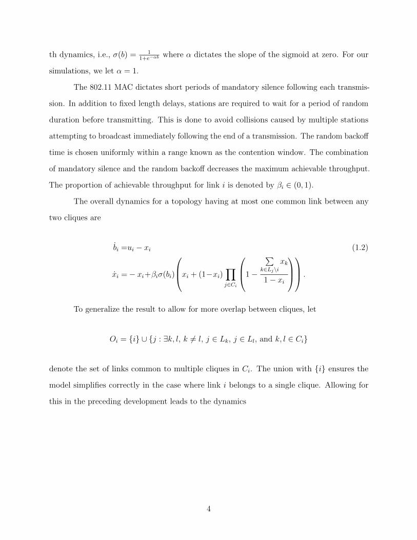
th dynamics, i.e., σ(b) = 11+e−αb

where α dictates the slope of the sigmoid at zero. For our

simulations, we let α = 1.

The 802.11 MAC dictates short periods of mandatory silence following each transmis-

sion. In addition to fixed length delays, stations are required to wait for a period of random

duration before transmitting. This is done to avoid collisions caused by multiple stations

attempting to broadcast immediately following the end of a transmission. The random backoff

time is chosen uniformly within a range known as the contention window. The combination

of mandatory silence and the random backoff decreases the maximum achievable throughput.

The proportion of achievable throughput for link i is denoted by βi ∈ (0, 1).

The overall dynamics for a topology having at most one common link between any

two cliques are

bi =ui − xi (1.2)

xi =− xi+βiσ(bi)

xi + (1−xi)∏j∈Ci

1−

∑k∈Lj\i

xk

1− xi

.

To generalize the result to allow for more overlap between cliques, let

Oi = {i} ∪ {j : ∃k, l, k 6= l, j ∈ Lk, j ∈ Ll, and k, l ∈ Ci}

denote the set of links common to multiple cliques in Ci. The union with {i} ensures the

model simplifies correctly in the case where link i belongs to a single clique. Allowing for

this in the preceding development leads to the dynamics

4

bi =ui − xi (1.3)

xi =− xi + βiσ(bi)

(xi +

∏j∈Oi

(1− xj)∏j∈Ci

1−

∑k∈Lj\Oi

xk

1−∑

k∈Oi∩Ljxk

.

Validation for this model can be found in [14], where Matlab simulations of various

topologies compare favorably to the results of packet-level ns-3 simulations.

1.2 Modeling Biological Networks

Now that we’ve established how to model wireless networks using differential equations, we

show how the same is possible for biological networks. First, we note that chemical reaction

networks describe a sequence of elementary chemical reactions, which are collisions of reactant

molecules that form certain products, absorbing and releasing energy in the process, [15],

[16]. A simple example of an elementary reaction would be:

X + Yk1−→ Z (1.4)

where X, Y, and Z are chemical species and k1 ∈ R+ is a number characterizing how quickly

or slowly the reaction takes place (small k1 describes a slow reaction, while large k1 describes

a fast reaction). For this chemical reaction, a molecule of X combines with Y to generate a

molecule Z at a rate of k1. We call X and Y the reactants, and Z the product of the reaction.

Chemical kinetic equations can be represented by a series of differential equations

by applying the law of mass action, which states that the rate of the forward reaction is

proportional to the product of the concentrations of the reactants, each raised to the power

of its coefficient in the balanced equation, [17]. It has been purported that the law of mass

action may not hold if the medium is not “well-mixed,” [16].

5

By applying the law of mass action, the chemical kinetics associated with the reaction

Equation 1.4 can be represented mathematically as follows:

x = −k1xy

y = −k1xy

z = k1xy

(1.5)

Note that there is a differential equation for each molecule, each defining how the concentration

of a molecule in the elementary reaction step changes over time. Chemical concentrations

of the chemical species X, Y, and Z are denoted by their lowercase counterparts x, y, and

z, respectively, using the systems biology notation as in [16]. The equivalent in traditional

chemistry is to denote the chemical concentrations using square brackets, so the chemical

concentration for X would be denoted [X].

If the reverse reaction of Equation 1.4 also occurred, Zk2−→ X + Y, then the series of

differential equations representing these chemical reactions becomes:

x = −k1xy + k2z

y = −k1xy + k2z

z = k1xy − k2z

(1.6)

The combination of Equation 1.4 with its reverse reaction can be simplified to the chemical

kinetic equation:

X + Yk1−⇀↽−k2

Z

Chemical reactions often involve more than one of the same molecule. The different

numbers of molecules that are necessary to form the desired compounds in various quantities

are called the stoichiometry of the reaction. For example, the chemical reaction 2 A + 3 Bk3−→ C

6

has stoichiometry 2 : 3 : 1 and is modeled by the series of differential equations:

a = −k3a2b3

b = −k3a2b3

c = k3a2b3

Using the above theory for chemical kinetics, we will now look at an example of a chemical

reaction network, which is essentially the interactions between a set of elementary reaction

steps.

Example 1. Consider the following set of chemical reactions:

A + Ek1−→ C

k2−⇀↽−k3

2 B + E

Under mass-action assumptions, these reactions suggest the following chemical kinetics:

a = −k1ae

b = k3b2e− k2c

c = k1ae− k3b2e+ k2c

e = −k1ae+ k3b2e− k2c

(1.7)

1.2.1 The Hill Equation

In order to complete our understanding of modeling biological systems using differential

equations we now add a quick note on the Hill equation. The Hill equation was first proposed

by A.V. Hill in 1910 in order to describe the equilibrium relationship between oxygen tension

and the saturation of haemoglobin [18]. More recently the Hill qeuation has been used for

other applications, such as describing the drug concentration-effect relationship, [19].

7

The general form of the Hill equation is a three parameter equation describing the

relationship between two variables, x (the independent variable) and y (the dependent

variable):

y =ymaxx

α

cα

the three parameters are ymax, c, and α, [19].

Since there are many possible uses of the Hill equation, we will focus now on just two

specific uses of the Hill equation that are prevalent today. The Michaelis-Menten equation,

[20], is a special example of the Hill Equation and describes the relationship between the

velocity of a reaction, v, and the concentration of a substrate, s, with the following expression:

v =(Vmax)s

Km + s

where v is the initial velocity, Vmax is the maximum reaction rate, s is the substrate concen-

tration and Km is concentration of substrate at which the rate of the enzymatic reaction is

half Vmax, [19].

Another important application of the Hill equation is with regards to physiochemical

equilibrium. Let us consider the notion of a single equilibrium reaction between two molecules,

L and M , and their combination, LM . This can be denoted using chemical reaction kinetics

as

L + M −−⇀↽−− LM.

The Hill equation defining y, the ratio of molecules of L that have reacted, is:

y =m

KD +m

where m is the concentration of the molecule M and KD represents the concentration ofM

for which y is equal to 0.5 (i.e. ymax2

).

8

This result can be extended for multiple binding patterns, such as multiple molecules

of a ligand binding to a receptor, by considering the following equilibrium:

Ln + nM −−⇀↽−− LnM.

The corresponding Hill equation then becomes:

yn =mn

Kn +mn.

1.3 Network Structure Representations

Thus we have shown that we can produce a series of differential equations representing the

the behavior of links in a wireless network as well as chemical kinetics of a biological network.

Once we have these systems of equations for our particular application, they can then be

stacked into vector to yield an equation of the form:

x = f(x). (1.8)

For example, the equations in (1.7) would become:

x =

a

b

c

e

and f(x) =

−k1ae

k3b2e− k2c

k1ae− k3b2e+ k2c

−k1ae+ k3b2e− k2c

In this particular case f(x) contains nonlinear functions. When the functions are

linear the equation in (1.8) becomes:

x = Ax, (1.9)

9

where A ∈ Rn×n is the matrix of coefficients, often referred to as the dynamics matrix, and

x ∈ Rn. The A matrix contains all the information about the structure of the network. When

there is an external input, u ∈ Rm, into the system and output, y ∈ Rp, from the system, the

nonlinear system is denoted:

x = f(x, u)

y = g(x, u)(1.10)

The linear equivalent of (1.10) is defined as:

x = Ax+Bu

y = Cx+Du(1.11)

where A is defined as in (1.9), B ∈ Rn×m is called the control matrix, C ∈ Rp×n is called the

sensor matrix, and D ∈ Rp×m is the direct term. Note that frequently systems will not have

a direct term, indicating that the control signal does not influence the output directly, [21].

Many systems, including wireless computer networks and biological networks, are

nonlinear, with behavior that is difficult to study. By linearizing the system in (1.10) around

an equilibrium point we can apply linear systems theory to understand the behavior of the

system close to this equilibrium. An equilibrium point is defined as a pair (xeq, ueq) ∈ Rn×Rk

such that f(xeq, ueq) = 0, resulting in x = 0. The local linearization around an equilibrium

point is the linear time-invariant system:

x = Ax+Bu

y = Cu(1.12)

where A = ∂f(xeq ,ueq)∂x

, B = ∂f(xeq ,ueq)∂u

and C = ∂g(xeq ,ueq)∂x

, where f and g are the equations

from (1.10), [22].

Note that for nonlinear systems, it is also possible that the system cycles through a

specific trajectory continuously, rather than staying at a specific point, until perturbed. This

type of phenomenon is referred to as a limit cycle. A limit cycle exists when a system has

10

a nontrivial periodic solution such that x(t+ T ) = x(t),∀t ≥ 0, also referred to as a closed

curve, [23]. If we let C be a closed curve, and if every trajectory moves asymptotically onto

C as t→∞, then C is called a stable limit cycle, shown in Figure 1.1a. If every trajectory

moves asymptotically onto C as t→ −∞, then C is called an unstable limit cycle, shown in

Figure 1.1b, [24].

Figure 1.1: (a) Stable limit cycle, (b) Unstable limit cycle

It is possible to linearize around the limit cycle in order to apply linear systems theory,

but the linearization process is beyond the scope of this thesis. It is sufficient to note that

nonlinear systems can be linearized about an equilibrium, point or cycle, in order to get

them into the form shown in Equation 1.11, [25]. From this point on we will ignore the

nonlinear dynamics of our applications and focus on results related to linear time-invariant

(LTI) systems. Once we have linearized our system about an equilibrium, its complete

computational structure can then be represented graphically.

1.3.1 Complete Computational Structure

The complete computational structure of the system, without taking into account the concept

of intricacy, [26], in (1.11) is defined as the graphical representation of the dependency among

input, state, and output variables that is in direct, one-to-one correspondence with the

system’s state space realization, denoted C . C is a weighted directed graph with vertex

set V (C ) and edge set E(C ). The vertex associated with the ith input is labeled ui for

11

i = 1, ...,m and the vertex associated with the jth state is labeled j for j = 1, ..., n. The edge

set contains an edge from node i to node j if the function associated with the label of node

j depends on the variable or input labeled node i. Edges that show the dependence of a

state on an input are denoted bj,i, while the edges showing dependence among states are

denoted aj,i. Note, in some cases auxiliary variables are used to characterize intermediate

computations, but since it is standard practice to eliminate auxiliary variables for simplicity,

we will ignore them.

Example 2. Consider the following system:

x1

x2

x3

x4

x5

x6

x7

x8

x9

˙x10

˙x11

˙x12

˙x13

=

a1,1 0 0 0 0 0 0 0 0 0 0 0 a1,13

0 a2,2 0 0 0 0 0 0 0 a2,10 0 0 0

0 0 a3,3 0 0 0 0 0 a3,9 0 0 a3,12 0

0 0 0 a4,4 0 0 0 a4,8 0 0 0 0 0

0 0 0 0 a5,5 a5,6 0 0 0 0 0 0 0

0 0 0 a6,4 0 a6,6 0 0 0 0 0 0 0

0 0 0 0 a7,5 0 a7,7 0 0 0 0 0 0

a8,1 a8,2 0 0 0 0 a8,7 a8,8 0 0 0 0 0

0 0 0 a9,4 0 0 0 0 a9,9 0 0 0 0

0 0 0 0 0 0 0 0 0 a10,10 a10,11 0 0

0 0 a11,3 0 0 0 0 0 0 0 a11,11 0 0

0 0 0 0 0 0 0 0 0 0 0 a12,12 0

0 0 0 0 0 0 0 0 0 0 0 0 a13,13

x1

x2

x3

x4

x5

x6

x7

x8

x9

x10

x11

x12

x13

+

0 0 0

b2,1 0 0

0 0 0

0 0 b4,3

0 0 0

0 0 0

0 0 0

0 0 0

0 0 0

0 0 0

0 0 0

0 b12,2 0

b13,1 0 0

u1

u2

u3

(1.13)

The complete computational structure associated with the system in Equation 1.13 is:

Figure 1.2: Complete Computational Structure

The complete computational structure describes both the system’s structure and

dynamics, but it can often be too complicated to understand the nature of the whole system

12

with this representation. In this case, simpler representations of the network, such as the

subsystem structure or signal structure, could be more useful, [26].

1.3.2 Subsystem Structure

Subsystem structure refers to the interconnection structure of the subsystems of a given

system. Given the system with realization (1.11) and associated computational structure,

the subsystem structure is a condensation graph, a graph created by collapsing several nodes

in the complete computational structure into a single node for each subsystem, S of C with

vertex set V (S ) and edge set E(S ) given by:

• V (S ) = {S1, ..., Sq} are the elements of an admissible partition of V (C ), where q is

the number of distinct subsystems, and

• E(S ) has an edge (Si, Sj), labeled yk, if E(C ) has an edge from some component of Si

to some component of Sj

We label the nodes of V (S ) with the transfer function of the associated subsystem, which

we also denote Si, and the edges of E(S ) with the associated variable from E(C ).

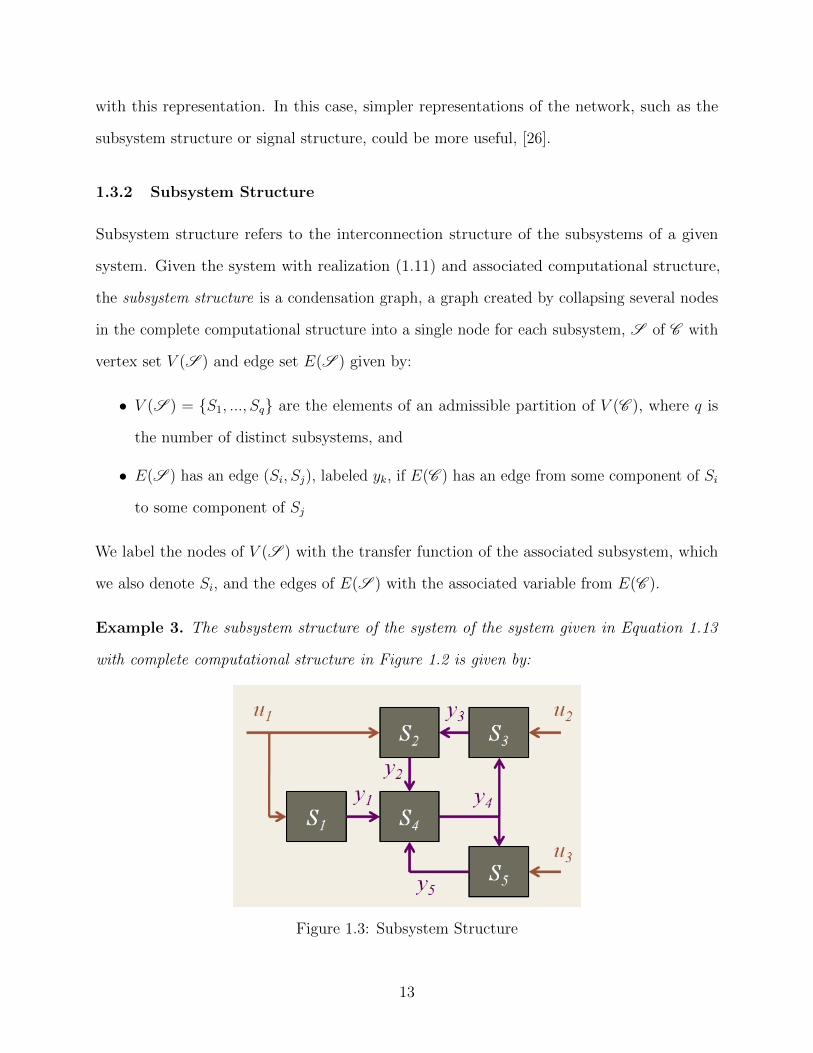
Example 3. The subsystem structure of the system of the system given in Equation 1.13

with complete computational structure in Figure 1.2 is given by:

Figure 1.3: Subsystem Structure

13

The subsystems in Figure 1.4 are S1 = {1, 13}, S2 = {2, 10, 11}, S3 = {3, 9, 12},

S4 = {4, 7, 8} and S5 = {5, 6}.

1.3.3 Signal Structure

Another natural way to partially describe the structure of a system is to characterize the

open-loop causal dependence among each of its manifest variables. The state space of the

system is shown in Equation 1.11 and we will consider the case when C =

[I 0

]. This will

split the state variables into two parts:

x1

x2

, where x1 contains the measured states and x2

contains the hidden states.

The full derivation for dynamical structure functions can be found in [26], but the

main result is:

X1 = Q(s)X1 + P (s)U (1.14)

where X1 and U are the Laplacians for x1 and u, respectively, Q(s) = (sI −D(s))−1(W (s)−

D(s)) and P (s) = (sI −D(s))−1V (s). Furthermore, W (s) =

[A11 + A12(sI − A22)−1A21

],

V (s) =

[B1 + A12(sI − A22)−1B2

]and D(s) is defined to be a diagonal matrix whose entries

are the diagonal values of W (s). The matrices (Q(s), P (s)) are called the dynamical structure

functions of the system.

The signal structure of a system with realization (1.11) and dynamical structure

function (Q(s), P (s)) characterized by (1.14), is a graph W , with a vertex set V (W ) and

edge set E(W ) given by:

• V (W ) = {u1, ..., um, y11, ..., y1p1 , y21, ..., y2p2}, each representing a manifest variable of

the system, and

• E(W ) has an edge from ui to y1j or y1i to y1j if the associated entry in P (s) or Q(s)

(as given in Equation (1.14)) is nonzero, respectively.

14

We label the nodes of V (W ) with the number of the associated variable, and the edges of

E(W ) with the associated transfer function entry of Q(s) or P (s) from Equation (1.14).

Example 4. The signal structure of the system in Equation 1.11 with complete computational

structure in Figure 1.2 is:

Figure 1.4: Signal Structure

With these different notions of structure defined, we can discuss how they each affect

the reconstruction process.

1.3.4 Network Reconstruction

The reconstruction process begins with data, usually input-output data, from the system and

attempts to determine the parameters of a model of the system. The first step, as shown in

Figure 1.5, is referred to as system identification.

The purpose of system identification is to determine the mathematical model of

input-output behavior of a system from data. This model is referred to as the system’s

transfer function, G, which represents the input-output relationship of a linear time invariant

system by:

y = Gu (1.15)

15

Data Models Reconstruction Realization

Identification

Transfer Function

Dynamical Structure Function

State Realization

Structural Informativity

G (Q,P) (A,B,C,D)

Figure 1.5: The Reconstruction Process

where u ∈ Rm is the input to a system and y ∈ Rp is the output of the system. G is a black

box representation of the system, containing no information about the structure. The system

identification process for determining a system’s transfer function from input-output data

has been well studied and there exist many methods for transfer function identification, [27].

The transition from a system’s transfer function to its state space form is called

realizing the system, as shown in Figure 1.5. Attempting to determine the state space

realization for a system given the system’s transfer function, G, is an ill-posed problem since

there are many state space realizations for a single transfer function matrix. The only way to

realize the system and yield the state space model is if the system has full state feedback,

meaning that every node in the system is measured. Since this is not generally possible for

biological networks, various assumptions are made about the system a priori before the state

space realization can be determined.

Thus, reconstructing the system to a partial structure representation, so that less extra

information is required, would be more desirable than attempting to realize the entire system.

The process of network reconstruction from a system’s transfer function to its subsystem

structure, (N,S), is known to be difficult, evidenced by the lack of literature in the field.

So, in order to reconstruct a biological network with weak a priori information, dynamical

structure functions were developed to represent the system’s signal structure.

16

Dynamical structure functions represent networks in terms of Q and P as defined

in (1.14). The relationship between a system’s dynamical structure function (Q,P ) and its

transfer function G is given by:

G = (I −Q)−1P

In [28], sufficient conditions for reconstruction of biological networks using dynamical structure

functions were shown for diagonal P . This work seeks to extend these results to determine

necessary and sufficient informativity conditions as well as detailing a methodology for robust

reconstruction of networks.

17

Chapter 2

Related Work

With the network reconstruction process detailed, it is also pertinent to understand

the various network reconstruction methods that are available. Improvements in technology

have led to the advent of a plethora of reconstruction algorithms that are being developed at

a rate that is doubling every two years, [29]. The flood of algorithms led to the creation of

the DREAM (Dialogue on Reverse Engineering Assessment and Methods) competition at

MIT, whose purpose it is to assess the performance of network reconstruction algorithms.

Available inference techniques include correlation-based methods (discussed in Section 2.1),

Bayesian network predictions (discussed in Section 2.2), and methods based on dynamical

models (discussed in Section 2.3), [29]. After looking at the reconstruction methods, we

discuss reconstruction as is relates specifically to the applications of biological systems in

Section 2.4 and wireless networks in Section 2.5.

2.1 Correlation Methods

The first attempts at network reconstruction came by way of correlation studies, which was

invented over a century ago by Francis Galton who stated that correlation between two

variables measured the extent to which the variables were governed by “common causes,”

[30]. Modern correlation methods attempt to determine correlations between species through

perturbation experiments, [31] and [32]. However, Karl Pearson and his assistant G. Udny

Yule, whose works came roughly a decade after Galton and who were instrumental in the

18

development of correlation analysis, discussed a limitation of correlation analysis, namely

“misleading,” or “spurious” correlations: which refers to variables A and B that are not

directly causally related, but are both effects of C, [33]. This reveals an inherent problem

in the application of correlation studies to network inference. While certain species may

appear correlated, that does not necessarily guarantee that connections exist between them.

Moreover, although there have been efforts to remove spurious connections after performing

the correlation analysis, it may not be possible to remove all the spurious edges in order to

determine the correct network, [34].

2.2 Bayesian Networks

In order to overcome the weakness of correlation methods, a popular technique for reconstruc-

tion has been to infer the probability of connections between species using Bayesian networks.

Bayesian networks are graphical models in which each node represents a random variable

and each edge represents the probabilistic dependence among the corresponding random

variables. The main problem with applying Bayesian networks to the network reconstruction

of biochemical networks is that their structure corresponds to a directed acyclic graph (DAG),

while cycles tend to appear frequently in biochemical and wireless networks, [35].

Due to this limitation, some researchers in biology have focused on network recon-

struction in areas of biology where DAGs are common, such as pedigree analysis, where the

distribution of a genotype depends on the genotype of its biological parents, or phylogenetic

models, which studies the probability of different evolutionary sequences occurring in species,

[36]. Wireless network researchers also tend towards problems where DAGs are prevalent,

such as the analysis of cognitive networks [37] or indoor positioning systems for location

estimation of wireless devices [38].

Another approach has been to use dynamic Bayesian networks, which are able to

handle cyclic networks by using time series information, [39]. However, inference using

dynamic Bayesian networks is slow, even when the network is sparse, since the minimum

19

size of the posterior distribution for any arbitrary time slice is generally exponential in the

number of variables that have parents in the previous slice, [40].

Many inference algorithms suffer from issues with time complexity, even network

reconstruction with DSF contains a combinatoric search when noise is present in the system

and robust reconstruction is necessary, although it has been shown that under certain

conditions this time complexity can be reduced to polynomial time, [41]. There have

been attempts by several researchers to rectify this issue, such as the Reverse Engineering

Algorithm developed in [42] which utilizes dynamical models and was developed specifically

for the reconstruction of large networks, but even that still has problems with computational

complexity.

2.3 Dynamic Models

Dynamic models are defined as models that take the following as input: (1) interactions

and regulatory relationships between components, (2) how the strength of the interactions

depends on the state of the interacting components and (3) initial state of each component

in the system, and produce as output the time evolution of the state of the system, [43].

Since the description of a dynamic model is so broad, they are often modeled with varying

degrees of detail and model flexibility. The highest level of detail are found in differential

equations and stochastic models, which contain the most information about the system

computationally demanding when attempting to reconstruct a network and often require

accurate measurements. At the other end of the spectrum lies promotion-inhibition networks,

which are incredibly simple in that they assume a chemical species is either on or off and

have the advantage of being easy to interpret and robust, [44].

The state space model, as outlined in Section 1.3, falls into the category of being

an extremely detailed dynamic model. As noted in Section 1.3.4, the realization of the

state space model from a system’s transfer function is ill-posed. In order to overcome this,

researchers attempted to find the state space that fit the assumption that the sparsest system

20

was the actual system, [45]. However, this is a poor assumption because “parsimony is not

the correct criterion for selection of biological regulatory networks since the evolution selects

the networks that are robust and redundant rather than parsimonious,” [46].

Another common assumption is that the structure of a system is known a priori

in a very strong sense, such as an entire partition of the overall state space is assumed

to be known, [47], [48]. However, while “assuming knowledge of such a partition may be

reasonable in some cases, especially when considering engineered systems... in other situations,

however, assuming a priori knowledge of a partition over the entire state space of the complex

system could be unreasonable. For example, when modeling a chemical reaction network of a

biological system,” [49]. Therefore, a more suitable network reconstruction technique would

require less a priori information.

A look at the other end of the spectrum are simplified models such as a promotion-

inhibition model in biological networks, [50]. While simple representations have their benefits,

their dynamics are often too strict. In the promotion-inhibition example, not every species in

a network can be measured, the connections between certain species may be promoting in

some instances and inhibiting in other instances, depending on the hidden variables in the

system. A more accurate model of the system would not compromise these dynamics.

The benefit of utilizing dynamical structure functions is that it requires only weak

a priori information when compared to the realization process, [49], and it contains more

information about the dynamics of the system than a simple promotion-inhibition graph.

Although current results only hold for a diagonal P , this thesis presents necessary and

sufficient conditions for network reconstruction even without assuming target specificity of

controlled inputs.

2.4 Direction of Research in Systems Biology

Having reviewed the reconstruction process in general, we now take a quick look at how systems

biology has been evolving in recent years, leading to a renewed interest in improvements

21

in the field, such as that of network reconstruction. In the preface to [51] the editors note

several reasons for increased interest in systems biology recently as well as the direction of

research in the area. Firstly, a greater understanding of molecular mechanisms has led to an

increased focus on cell physiology. Secondly, experimental techniques have improved, allowing

for new opportunities for investigating cellular behavior, including new “high-throughput”

technologies allowing for the analysis of system-wide behavior.

According to [52], computational modeling and analysis have now become useful in

providing useful biological insights and predictions for well understood such as the bifurcation

analysis of the cell cycle, metabolic analysis or comparative studies of robustness of biological

oscillation circuits. This is not only because of improvements in biological experiments and the

understanding of cell structure, but also because of advances in software and computational

power has enabled the creation and analysis of reasonably realistic yet intricate biological

models.

2.5 Interference Maps for Wireless Networks

Just as improved technology has helped in systems biology, it has been imperative in

the development of wireless network technology. As noted in [14] wireless networking is

increasingly being used to deploy enterprise LANs and multi-hop mesh networks, especially

in rural areas. One of the difficulties that arises in deploying and maintaining a wireless

network is dealing with contention and interference, which can cause performance degradation,

[53–55].

One way to manage contention and interference in a wireless network is to develop an

interference map of the network [11, 56]. Using the interference map a network manager can

then rearrange nodes in order to reduction contention and interference, [57, 58].

There are two main approaches for developing an interference map of a wireless

network. The first approach uses controlled offline experiments, measuring the contention

between two nodes at a time in the network, [11, 56, 59]. Using broadcast measurements,

22

this approach only requires experiments on the order of O(n2) [11, 56]. One attempt of this

approach reduced the complexity to O(n), but ignored remote interferers, [59], although

it has been shown that remote interferers are the main source of interference in a wireless

network, [11].

The second approach for developing an interference map uses online, passive measure-

ments of the network to determine contention and interference relationships. Some attempts

of this approach have used packet sniffing, [60, 61]. However, one disadvantage of using packet

sniffing is that nodes must be synchronized. Another attempt at this approach collected traffic

from existing network flows, then used regression analysis to infer relationships among them

[62]. However, this technique is unable to distinguish between direct and indirect relationships.

Another online method is known as microprobing, where two nodes are synchronized to

simultaneously send a small probe packet in order to determine the relationship between

them, [63].

This thesis presents a method for determining a type of interference map of a wireless

network, in this case the open-loop causal dependencies between sending rates on links, i.e.

how the sending rate of one link affects the rates of other links. The benefit of the method

presented is that we can create the map while the network is online and we are able to detect

the presence of transitory unidentified nodes and devices which are not part of the managed

structure.

23

Chapter 3

Foundational Material

Before delving into the new results, we begin by outlining the evolution of the network

reconstruction process associated with Dynamical Structure Functions. First, we note that

the dynamical structure function (Q, P ) is not uniquely specified for a given transfer function

G without a priori information. Thus, we require informativity conditions that state exactly

what information about the network is required so that the pair (Q, P ) is uniquely specified.

In [28] sufficient informativity conditions were given for reconstruction when no noise is

present within the system, discussed in Section 3.1.

Having shown that reconstruction was possible under certain conditions without

noise present in the system, [1] presents two robust reconstruction techniques allowing for

reconstruction when noise is present in the system. The first reconstruction technique

calculates Q and P from G while the other reconstructs directly from input-output data. In

Sections 3.2 and 3.3 we outline each method, as well as the advantages and disadvantages of

each.

Finally, in Section 3.4 we highlight an important aspect of the robust reconstruction

process: using an information criterion to penalize extra connections. This is useful in the

reconstruction process since the robust reconstruction methods tend to favor networks that

contain more links, even when the actual network is sparse.

24

3.1 Sufficient Informativity Conditions for Network

Reconstruction

Sufficient informativity conditions for network reconstruction with dynamical structure

functions was outlined in [28], first noting that reconstruction without a priori information

about the system was not possible in the following theorem:

Theorem 1. Given any p ×m transfer function G, with p > 1 and no other information

about the system, dynamical and Boolean reconstruction. Moreover, for any internal structure

Q, there is a dynamical structure function (Q,P ) that is consistent with G.

The sufficient conditions for reconstruction, noting what a priori information allowed

for reconstruction, were then outlined in the following theorem:

Theorem 2. Given a p × m transfer function G, dynamical structure reconstruction is

possible from partial structure information if p− 1 elements in each column of

[Q P

]′are

known that uniquely specify the component of (Q,P ) in the nullspace of

[G′ I

].

Using these sufficient conditions, the authors of [28] noted that a diagonal P is a

sufficient condition for reconstruction in the following corollary:

Corollary 1. If m = p, G is full rank, and there is no information about the internal

structure of the system Q, then the dynamical structure can be reconstructed if each input

directly controls a measured state independently (i.e., without loss of generality, the inputs

can be numbered such that P is diagonal). Moreover, H = G−1 characterizes the dynamical

structure as follows:

Qij = −Hij

Hii

and Pii =1

Hii

.

A system with diagonal P , as this corollary notes, is one one where each measured

state can be independently controlled. This sufficient condition for reconstruction severely

restricted the systems that could be reconstructed. This thesis extends these results to show

25

exactly what information is necessary and sufficient for reconstruction, even when P is not

diagonal. Note that this does not mean that we can reconstruct every network, we simply

determine under what conditions a system can be reconstructed without the restriction that

P is diagonal.

3.2 Robust Reconstruction from G

While we can solve for Q and P exactly from G under the conditions in Corollary 1, finding

Q and P exactly is almost impossible for real or simulated systems when noise is present in

the system. So, in [1], it was shown that if noise is present, one can determine the dynamical

structure function from a stable transfer function G using a robust reconstruction method

when P was diagonal.

First, the transfer function is identified from noisy time-series data using standard

system identification tools, [64]. Since noise is present in the system, reconstructing perfectly

from G is no longer possible using Corollary 1 since the noise would lead to a dynamical

structure function in which the internal structure function Q would appear to be fully

connected, even if it wasn’t. In order to overcome this, the distance from G to all possible

boolean structures (of which there are 2p2−p of them) is quantified. Structures with small

distances are candidates for the correct structure of the network, while those that have large

distances associated with them are unlikely to be the correct structure, a thresholding process

is used to determine what constitutes “small” and what constitutes “large”.

There are many ways to model input-output data with noise and nonlinearities, in

[1] a feedback uncertainty on the output was considered as it yielded a convex optimization

problem, [65]. Using this framework, the true system is given by (I + ∆)−1G, where ∆

represents unmodelled dynamics, such as noise and nonlinearities. Given the true system, the

distance from data to a particular Boolean structure is chosen by minimizing ||∆|| such that

Q obtained from (I + ∆)−1G = (I −Q)−1P has the desired Boolean structure. Solving for

∆, we can rewrite the above equation as ∆ = GP−1(I −Q)− I. Letting X = P−1(I −Q),

26

the Boolean structure constraint on Q can be reformulated on X, i.e., non-diagonal zero

elements in X correspond to those in Q since Xij = P−1ii Qij for i 6= j.

Now ordering all Boolean structures from 1 to 2p2−p, and defining a set χk containing

transfer function matrices that satisfy the following conditions: (i) for i 6= j, Xij(s) = 0 if for

the considered kth Boolean structure Qij(s) = 0; all other Xij(s) are free variables; (ii) when

i = j, Xii(s) is a free variable. The distance from G to a particular Boolean structure can be

written as αk = infX∈χk ||GX − I||2, which is a convex minimization problem with a careful

choice of norm. Next, we show that this problem can be cast as a least squares optimization

problem. If we use the norm defined by ||∆||2 = sum of all ||∆ij||22, where || · ||2 stands as

the L2-norm over s = jω, then using the projection theorem [66] the problem reduces to:

αk =∑i

||Ai(A∗iAi)−1A∗i ei − ei||22

where Ai is obtained by deleting the jth columns of G when the corresponding elements Xi[j]

are 0 for all j, and (·)∗ denotes transpose conjugate.

3.3 Robust Reconstruction from Data

Although the previous method for robust reconstruction works well, information can be lost

when determining a system’s transfer function G from data and then reconstructing to find

the dynamical structure function (Q,P ) from G. Thus, another method was also proposed

in [1] that allows for the reconstruction of the dynamical structure function (Q,P ) directly

from data. Rather than feedback uncertainty, this method considers additive uncertainty on

the output, i.e., Y = G∆(U + ∆). In this case, the distance is how much the input much be

changed in order for the reconstructed system to fit a particular Boolean structure. Since

G∆ = (I −Q)−1P = X−1, the equality Y = G∆(U + ∆) can be written as

∆ = XY − U,

27

where X ∈ χk for some particular Boolean network k. Recall that structural constraints in

Q can be imposed directly on X from the equality X = P−1(I − Q). Then, using system

identification tools for non-causal auto-regression models under the structural constraints

one can identify X (which might be non-causal). In this case the distance is defined as the

maximum likelihood of the estimation problem.

3.4 Penalizing Connections using an Information Criterion

While the two robust reconstruction methods are theoretically sound, there is an inherent

flaw associated with both of them. Namely, that there are several candidate structures with

distances smaller than the true structure of the system. For example, since the fully connected

network has extra degrees of freedom its corresponding distance αk is the smallest of all.

This is similar to the problem of noisy data over-fitting encountered in system identification

when attempting to determine the correct transfer function of a system, where a higher order

transfer function yields a better fit. The typical approach in system identification to pick

a more correct transfer function is to penalize higher dimensions and the analogy in the

network reconstruction case is to penalize extra network connections, [1].

Consider the case that the true network has l non-existent connections, i.e. l off-

diagonal elements in Q are zero, then there are 2l − 1 different Boolean networks that have

a smaller or equal distance due to the extra degrees of freedom provided by the additional

connections for those network structures. In the case when noise is present, the true network

structure will typically have a distance similar to those other l structures. The question of how

to find the true network from among these candidate structures then arises. With repeated

experiments, small enough noise (i.e., large enough signal-to-noise ratio) and negligible

nonlinearities, the distances associated with those l networks are comparable, and they are

usually much smaller than those of the other networks.

Now, in order to determine the correct network structure, one must find a balance

between network complexity and data fitness by taking into account the associated distance

28

along with penalizing extra connections. There are several ways to do this, one of which

is Akaikes Information Criterion (AIC) [67], or some of its variants such as AICc, which is

AIC with a second correction for small sample sizes, and the Bayesian Information Criterion

(BIC) [68].

AIC is tool for model selection, so, given a data set, several competing models may

be ranked according to their AIC value, with the one having the lowest AIC being the best

model. The AIC value for a particular Boolean network Bk is defined in [1] as

AICk = 2Lk + 2ln(αk),

where Lk is the number of (non-zero) connections in the Boolean network Bk and αk is the

optimal distance for this Boolean network.

29

Chapter 4

Necessary and Sufficient Informativity Conditions

As noted in Section 3.1, previous results only provided sufficient informativity condi-

tions for the reconstruction of a network. The first contribution of this thesis are conditions

that are both necessary and sufficient for network reconstruction using dynamical structure

functions, found in Section 4.1. Having established the necessary and sufficient informativity

conditions, in Section 4.2 several examples of the reconstruction of dynamical structure

functions utilizing these conditions are detailed.

4.1 Necessary and Sufficient Conditions for Network Reconstruc-

tion

As in Section 3.2, we will assume that the system’s transfer function has been successfully

identified from data using standard system identification tools, [64]. Thus, we will focus

on necessary and sufficient informativity conditions that detail exactly what information is

needed a priori to ensure that for a given transfer function G the corresponding dynamical

structure function (Q,P ) is uniquely specified. To accomplish this, we will construct a

mapping from the elements of the dynamical structure function to the associated transfer

function and establish conditions to ensure this mapping is injective.

To facilitate the discussion, we introduce the following notation. Let A ∈ Cn×m and

B ∈ Ck×l. Then:

30

• blckdiag(A,B) is the block diagonal matrix given by

A 0

0 B

,

• ai is the ith column of matrix A,

• A−i is the matrix A without it’s ith column,

• aij is the (i, j)th entry of matrix A,

• A′ is the conjugate transpose of matrix A,

• R(A) is the range of A,

• −→a is the vector stack of the columns of A, given by

a1

a2

...

am

• and ←−a is the vector stack of the columns of A′.

The construction of a map from elements of the dynamical structure function to the

associated transfer function begins by rearranging Equation (4.1) from the following Lemma,

which was proven in [69]:

Lemma 1. The transfer function, G, of the system

y

x

=

A11 A12

A21 A22

y

x

+

B1

B2

u, y =

[I 0

] y

x

, is related to its dynamical structure, (Q,P ), by

G = (I −Q)−1P (4.1)

31

to get:

[I G′

] P ′

Q′

= G′ (4.2)

Noting that

AX = B ⇐⇒ blckdiag(A, ...,A)~x = ~b

and defining X =

[P ′ Q′

]′then allows us to rewrite Equation (4.2) as

[I blckdiag(G′, ..., G′)

]←−x =←−g . (4.3)

Further noting that since the diagonal elements of Q are identically zero and the dimensions

of P , Q, and G are p × m, p × p, and p × m respectively, then exactly p elements of ←−x

are always zero. Abusing notation, we can then redefine ←−x to remove these zero elements,

reducing Equation (4.3) to the following:

[I blckdiag(G′−1, G

′−2, ..., G

′−p)

]←−x =←−g . (4.4)

Equation (4.4) reveals the mapping from elements of the dynamical structure function,

contained in←−x , to its associated transfer function, represented by←−g . The mapping is clearly a

linear transformation represented by the matrix operator


′−2, ..., G

′−p)

].

This matrix has dimensions (pm)× (pm+ p2 − p), and thus the transformation is certainly

not injective. This is why not even the Boolean structure of a system’s dynamical structure

function can be identified – even from perfect information about the system’s transfer function

– without additional a priori structural information.

Identifiability conditions will thus be established by determining which elements of ←−x

must be known a priori in order to reduce the corresponding transformation to an injective

32

map. To accomplish this, consider the (pm+ p2 − p)× k transformation T such that

←−x = Tz (4.5)

where z is an arbitrary vector of k transfer functions.

Lemma 2. Let

M = LT, (4.6)

where L =


′−2, ..., G

′−p)

]and T is a (pm+ p2 − p)× k matrix operator

as in Equation (4.5). Then M is injective if and only if rank(M) = k.

Proof. This stems from the fact that M is a pm× k matrix, and M is injective iff it has full

column rank, meaning rank(M) = k.

Theorem 3. (Identifiability Conditions) Given a system characterized by the transfer function

G, its dynamical structure function (Q,P ) can be identified if and only if

1. M , defined as in Equation (4.6), is injective, and

2. ←−g ∈ R(M).

Proof. The proof follows immediately from the observation that M is the mapping from

unidentified model parameters to the system transfer function, i.e. Mz =←−g . Under these

conditions one can clearly solve for z given G and then construct the dynamical structure

function.

4.2 Necessary and Sufficient Informativity Conditions Examples

We will now illustrate this reconstruction result on some simple examples.

33

Example 5. Consider a system with square transfer function given by

G =

G11 G12 ... G1p

G21 G22 G2p

.... . .

...

Gp1 Gp2 ... Gpp

.

Previous work has shown that if G is full rank and it is known, a priori, that the control

structure P is diagonal that reconstruction is possible [69]. Here we validate that claim by

demonstrating that the associated T matrix becomes:

P11

P12

...

P21

P22

...

Ppp

Q12

...

Qp(p− 1)

=

1 0 ... 0 0

0 0 ... 0 0

......

. . ....

0 0 ... 0 0

0 1 ... 0 0

.... . . . . .

...

0 ... 1 ... 0

0 ... 0 1 0

.... . .

.... . .

...

0 ... 0 0 1

P11

P22

...

Ppp

Q12

...

Qp(p−1)

yielding the operator M = LT as:

M =

e1 0 0 G′−1 ... 0

0. . . 0 0

. . . 0

0 ... ep 0 ... G′−p

34

where ei is a zero vector with 1 in the ith position. Note that M is a square matrix with

dimensions p2× p2 and will be invertible provided G is full rank, thus enabling reconstruction.

Example 6. Given the following transfer function of a system:

G =

s+2s2+3s+1

− s2+3s+3(s+2)(s2+3s+1)

s+2(s+1)(s2+3s+1)

s2+s−1(s+1)(s2+3s+1)

We attempt to find the dynamical structure functions (Q,P ) of the system:

Q =

0 Q12

Q21 0

and P =

P11 P12

P21 P22

yielding the vector of unknowns ~x =

[P11 P12 P21 P22 Q12 Q21

]′. This gives us the

system of equations of the form L~x = ~b:

1 0 0 0 s+2(s+1)(s2+3s+1)

0

0 1 0 0 s2+s−1(s+1)(s2+3s+1)

0

0 0 1 0 0 s+2s2+3s+1

0 0 0 1 0 − s2+3s+3(s+2)(s2+3s+1)

P11

P12

P21

P22

Q12

Q21

=

s+2s2+3s+1

− s2+3s+3(s+2)(s2+3s+1)

s+2(s+1)(s2+3s+1)

s2+s−1(s+1)(s2+3s+1)

Without additional information a priori structural information, we can not reconstruct.

Suppose, however, that we know a priori that P takes the form:

P =

P11 −P11

0 P22

35

Note that this non-diagonal P fails to meet the previous conditions for reconstruction [69], [1].

Nevertheless, the vector of unknowns ~x can then be decomposed into the form T~z as follows:

T =

1 0 0 0

−1 0 0 0

0 0 0 0

0 1 0 0

0 0 1 0

0 0 0 1

and ~z =

[P11 P22 Q12 Q21

]′

Replacing ~x with T~z above yields the system of equations of the form M~z = ~b, where M = LT :

1 0 s+2(s+1)(s2+3s+1)

0

−1 0 s2+s−1(s+1)(s2+3s+1)

0

0 0 0 s+2s2+3s+1

0 1 0 − s2+3s+3(s+2)(s2+3s+1)

P11

P22

Q12

Q21

=

s+2s2+3s+1

− s2+3s+3(s+2)(s2+3s+1)

s+2(s+1)(s2+3s+1)

s2+s−1(s+1)(s2+3s+1)

In this case M is full rank, from Theorem 3 we know that the system is reconstructible. By

solving for ~z = (M)−1~b we get the DSF to be:

Q =

0 1s+2

1s+1

0

and P =

1s+1

− 1s+1

0 1s+2

The signal structure of the system is shown in Figure 4.1

36

u1

u2

y2

y1

Figure 4.1: Simple Two-Node Network with Non-Diagonal P

37

Chapter 5

Robust Network Reconstruction

Now that we have shown that it is possible to reconstruct a system when P is not

diagonal, we need new results to show how to reconstruct a system with non-diagonal P

when noise is present in the system. First, we define the robust reconstruction problem in

Section 5.1, which prepares us to develop a robust reconstruction algorithm for solving the

problem in Section 5.2. Given a robust reconstruction algorithm, in Section 5.3 we conclude

with examples of robust reconstruction for both diagonal and non-diagonal P .

5.1 Robust Reconstruction Problem

We begin by considering an additive uncertainty on the control structure P , as seen in Figure

5.1. Note that additive uncertainty over Q or both Q and P would be more interesting to

consider, but since they do not appear to produce convex minimization problems we are still

investigating their properties. Any results involving them will be the product of future work.

Figure 5.1: Additive uncertainty on P

38

The relationship we get from the block diagram in Figure 5.1 is Y = (I−Q)−1(P+∆)U ,

where ∆ represents noise and nonlinearities. Multiplying both sides by I−Q we get Y −QY =

(P + ∆)U . Then, if we solve for ∆U , we get ∆U = Y −QY −PU . This result is equivalent to

∆U = Y −[Q P

]YU

. Since U is a diagonal matrix, ||∆U || = ||c∆I|| = ||c∆|| = |c|||∆||,

where c 6= 0 is the amount each input is perturbed. Thus, we note that minimizing ||∆U ||

is equivalent to minimizing ||∆||, so to minimize the noise on the system, we minimize the

norm:

α = ||Y −[Q P

]YU

||Stacking the unknowns from Q and P into a vector d, this can be written as w −Md,

where w is the matrix Y stacked into a vector row by row and

M =

y2 ... yn 0 ... ... 0 u1 ... un 0 ... ... 0

0 ... 0. . . 0 ... 0 0 ... 0

. . . 0 ... 0

0 ... ... 0 y1 ... yn−1 0 ... ... 0 u1 ... un

(5.1)

where yi and ui are the ith columns of Y T and UT , respectively.

Therefore, we have reorganized the problem so that the norm we minimize is now

||w−Md||, which can be solved using least squares. Note, when the system has measurement

or sensor noise, both w and M will contain noise (since elements of Y are contained in both

w and M). The problem then becomes the minimization of:

α = ||(w + e1)− (M + e2)d|| (5.2)

where e1 and e2 represent noise in the system. This new representation of the problem can

then be solved using total least squares.

39

5.2 Robust Reconstruction Algorithm

The first step of implementation, given the input u and output y is to determine the z-

transform of each to yield Y (z) and U(z). We do this using the finite z-transform, which is

defined as:

X(z) =N∑k=0

x[k]z−k

Now that we have Y (z) and U(z), we can create M(z) as defined in Equation 5.1.

Next, we find every possible Boolean structure for the unknowns of Q and P , that fit

the a priori information given. For each structure we do the following:

1. Use the a priori information combined with information about the current Boolean

structure to restructure M . To do this, we create the matrix T defined in Equation

(4.5). Then, the matrix MT incorporates the a priori information about the network.

We then remove the columns of MT that correspond to the current Boolean structure.

2. For a large number of points on the unit circle, calculate α as given in 5.2, using total

least squares (discussed in Section 5.2.1). Note, in theory total least squares would

appear to yield better results, but in practice least squares works well. Thus, for the

current Boolean structure, there will be a large number of α values associated with

each point from the unit circle from which it was calculated.

3. Return the largest α value for the current Boolean structure.

Given an α for each boolean structure, we then use an information criterion to penalize

connections (discussed in Section 5.2.2). The boolean structure with the smallest information

criterion value should be the correct structure of the network.

40

5.2.1 Total Least Squares

The linear approximation problem AX ≈ B, where A ∈ Rm×n, X ∈ Rn×d, B ∈ Rm×d,

specified by

minX,E,G

||[ G | E ]||F subject to (A+ E)X = B +G

is called the total least squares (TLS) problem with the TLS solution XTLS ≡ X and the

correction matrix [ G | E ], with G ∈ Rm×d, E ∈ Rm×n.

Total Least Squares Solution

The solution to the Total Least Squares problem, as detailed in [70], is as follows: let UΣV T

be the SVD of the matrix [ B | A ], where U−1 = UT , V −1 = V T , Σ = diag(σ1, ..., σs, 0),

s ≡ rank([B|A]) with the partitioning given by Σ =[Σ

(∆)1 Σ

(∆)2

], where Σ

(∆)1 ∈ Rm×(n−∆),

Σ(∆)2 ∈ Rm×(d+∆), and V =

V (∆)11 V

(∆)12

V(∆)

21 V(∆)

22

where V(∆)

11 ∈ Rd×(n−∆), V(∆)

12 ∈ Rd×(d+∆), V(∆)

21 ∈

Rn×(n−∆), V(∆)

22 ∈ Rn×(d+∆).

Furthermore, ∆ ≡ κ, 0 ≤ κ ≤ n, where κ is the smallest integer such that:

1. the submatrix V(κ)

12 is full row rank, and

2. either σn−κ > σn−κ+1, or κ = n.

Then X(κ) = −V (κ)22 V

(κ)†12 is the solution of the system (A + E)X = B + G, where †

denotes the Moore-Penrose pseudoinverse of a matrix.

Total Least Squares Algorithm

The algorithm for solving the Total Least Squares, using the aforementioned solution, is given

in [70] as the following:

41

00: Set j = 0

01: If rank(V(j)

12 ) = d and j = n, then goto line 05

02: If rank(V(j)

12 ) = d and σn−j > σn−j+1, then goto line 0503: Set j = j + 104: Goto line 0105: Set κ = j

06: Compute X(κ) = −V (κ)22 V

(κ)†12

07: Return κ, X(κ)

Table 5.1: Total Least Squares Algorithm

5.2.2 Penalizing Connections using an Information Criterion

As mentioned previously, finding optimal α yields a series of candidate solutions because

network structures with more degrees of freedom than the true network have low values for

α. In previous work, [1], Akaike’s Information Criterion (AIC) was used to penalize the extra

connections, where AIC is defined as:

AIC = 2k − 2ln(L)

where k is the number of parameters in the model and L is the maximized value of the

likelihood function for the model.

Akaike’s Information Criterion with correction for finite sample sizes is defined as:

AICc = AIC +2k(k + 1)

n− k + 1

where n is the sample size.

Applying the AIC to our reconstruction algorithm did not yield good results, since

it favored the full Boolean structure too heavily. By observing α values of reconstructed

networks, we determined a variation of the AIC that can be used to find the correct Boolean

structure. We call this information criterion Vasu’s Information Criterion (VIC) and Vasu’s

42

Information Criterion with correction for finite sample sizes (VICc):

V IC = 10k + α (5.3)

V ICc = V IC +10k(k + 1)

n− k − 1(5.4)

where k and n are defined the same as in Akaike’s Information Criterion.

The coefficients were chosen so as to ensure that structures with large numbers of

connections were heavily penalized, while still taking into account the importance of the

smallest distance on the discovery of the true structure. Further discussion on how the VIC

and VICc was developed is found in Section 7.1

5.3 Robust Reconstruction Examples

We now present several examples for both diagonal and non-diagonal P . Note, in these

examples the system is searching for the boolean structure of Q only (we assume the structure

of P is known) since it is not unreasonable to assume that you know how you can affect the

network.

5.3.1 Example 1: Diagonal P

First, we simulate the linearized single feedback loop from [1] as shown in Figure 5.2, by

performing three experiments and perturbing each input.

The linearized state space equations of the single feedback loop are as follows:

43

u1

u3 u2

y3 y2

y1

Figure 5.2: Single Feedback Loop with Diagonal P

x1 = −x1 − .2289x6 + u1

x2 = −2x2 + 1.5x4 + u2

x3 = −1.5x3 + 0.5x5 + u3

x4 = 0.8x1 − 0.5x4

x5 = 1.2x2 − 0.8x5

x6 = 1.1x3 − 1.3x6

(5.5)

The results of each perturbation experiment are seen in Figure 5.3.

(a) First PerturbationExperiment

(b) Second PerturbationExperiment

(c) Third PerturbationExperiment

Figure 5.3: Linearized Single Feedback Loop Simulation Results

44

Running our algorithm, we get the results in Table 5.2, which have been sorted by

alpha from largest to smallest. Only a small number of the possible structures are shown in

the table since it contains all the relevant data for determining the best structure. The true

network is marked in red, while the network chosen using VICc is shown in pink.

Boolean Structure ...

0 1 01 0 11 1 0

0 0 11 0 00 1 0

0 1 11 0 00 1 0

...

0 1 11 0 11 1 0

Alpha (α) ... 457.7 0.002166 0.002127 ... 2.4× 10−26

VICc ... 607.7 54 90 ... 270

Table 5.2: Diagonal P without Noise

Note that the V ICc is lowest for the correct network. While this is not proof that our

algorithm is correct, it is evidence that the robust method works on certain networks when

noise is not present in the network. This result is preparatory for a more vigorous analysis,

which will be conducted in Chapter 7.

5.3.2 Example 2: Diagonal P with Noise

Using the same linearized single feedback model from Equation 5.5, but with measurement

noise added, we get the simulation results seen in Figure 5.4. The noise variance for this test

was 1× 10−3.




Figure 5.4: Linearized Single Feedback Loop with Noise Simulation Results

45

Running our algorithm, we get the results shown in Table 5.3, which have been sorted

by alpha from largest to smallest. Again, only a subset of the candidate structures are shown

since it contains all the relevant data needed to determine the best structure. The true

network is marked in red and the lowest VICc value is marked in pink.


0 1 01 0 11 1 0

0 0 11 0 00 1 0

0 1 11 0 00 1 0

...

0 1 11 0 11 1 0

Alpha (α) ... 501.5 4.31 4.054 ... 5.05× 10−26

VICc ... 651.5 58.31 94.05 ... 270

Table 5.3: Diagonal P with Noise

The true system still retains the lowest V ICc and, as noted previously, while this is

not a formal proof or validation that the robust method is correct, it illustrates that the

algorithm appears to be working correctly, even when noise is present within the system.

5.3.3 Example 3: Non-Diagonal P

To illustrate that our algorithm works even with non-diagonal P , we begin with something

simple, using a slight variation on the simple feedback loop, as can be seen in Figure 5.5.

u1

u3 u2

y3 y2

y1

Figure 5.5: Single Feedback Loop with Diagonal P

46

The state space equations of the non-diagonal P feedback loop are the same as those

in Equation (5.5), except for the definition of x2 which is defined as:

x2 = −2x2 + 1.5x4 − u1 + u2 (5.6)

Simulating the system without noise yields the results seen in Figure 5.6.




Figure 5.6: Linearized Single Feedback Loop with Non-Diagonal P Simulation Results

Running our algorithm, we get the results shown in Table 5.4, which has again been

sorted by alpha from largest to smallest. Only relevant data for determining the best structure

is shown. The true network is marked in red with the lowest VICc score marked in pink.


0 1 01 0 11 1 0

0 0 11 0 00 1 0

0 1 11 0 00 1 0

...

0 1 11 0 11 1 0

Alpha (α) ... 145.2 0.001528 0.001517 ... 8.681× 10−27

VICc ... 295.2 54 90 ... 270

Table 5.4: Non-Diagonal P without Noise

Note that the V ICc is again lowest for the true network, this is promising because

we have now shown that our robust results extend beyond the previously reconstructible

networks that required P to be diagonal, at least for the example of this network with no

noise present.

47

5.3.4 Non-Diagonal P with Noise

Simulating the system in Equation (5.6) with measurement noise gives us the results seen in

Figure 5.7. As in the case with the diagonal P network, the noise variance for this test was

1× 10−3.




Figure 5.7: Linearized Single Feedback Loop with Non-Diagonal P and Noise SimulationResults

Running our algorithm, we get the results shown in Table 5.5, which have again

been sorted by alpha from largest to smallest. Only relevant data for determining the best

structure is shown. The true network is marked in red and the lowest VICc score is given in

pink.


0 1 01 0 11 1 0

0 0 11 0 00 1 0

0 1 11 0 00 1 0

...

0 1 11 0 11 1 0

Alpha (α) ... 168.5 8.301 6.377 ... 5.665× 10−27

VICc ... 318.5 62.3 96.38 ... 270

Table 5.5: Non-Diagonal P with Noise

In this final example, the AICc is again lowest for the true network, so we have shown

that for both diagonal and non-diagonal P with and without noise, reconstruction is possible.

Before we begin a thorough analysis of the new reconstruction method, we first present the

Matlab toolbox that implements the robust network reconstruction algorithm. This Matlab

48

toolbox was used to generate the examples in this chapter and will be helpful in facilitating

an analysis of the reconstruction algorithm.

49

Chapter 6

Matlab Toolbox

The Matlab toolbox developed for this thesis implements the robust reconstruction

algorithm described in Chapter 5. A list of the functions created for this toolbox are outlined

in Section 6.1. Then, in Section 6.2 verification of the various functions outlined is conducted.

The code fore each of the functions can be found in the Appendix (Chapter 12).

6.1 List of Functions

Table 6.1 contains a list of all the functions that are available in the Matlab toolbox.

Function Name Input Output Purpose of Function

createDiag Size N Coefficient cell ma-

trices Qcoff and

Pcoff , and their

corresponding un-

knowns they mul-

tiply, Qstruct and

Pstruct, along with

the total number

of unknowns in Q

and P , count1 and

count2

This function creates

the basic structure con-

straints for a diagonal P

system. Can be edited

to create other networks,

such as non-diagonal P ,

easily.

50

findT Qcoff , Qstruct,

Pcoff , Pstruct,

count1 and

count2

The a priori infor-

mation about the

network, T

This function takes in a

priori information about

the network and creates

the matrix T

robustRecon A priori informa-

tion, T , input-

output data, y

and u, number

of unknowns in

Q and P , N

and C, flag stat-

ing whether or

not to display α

and V ICc val-

ues, displ

Dynamical Struc-

ture Functions Q

and P

Given input-output data

and a priori information

about the network, this

function returns the pro-

posed Boolean structure

of the network

findAlphas T , y, u, N A list of alpha val-

ues aalpha

Given information about

the network, this function

returns the alpha values

associated with each pos-

sible Boolean structure

findCombs N List of all possi-

ble Boolean struc-

ture allQ

Creates a list of all pos-

sible Boolean structures

based on the number of

unknowns in Q

51

getAlpha T , y, u, allQ{i} Alpha α Given a Boolean struc-

ture, this function finds

it’s α value

zTransform A vector f and a

point on the unit

circle z

F , the z-transform

of f

Determines the z-

transform of a vector f

at the point z

findM Y , U The matrix M Given the z-transforms Y

and U , we now find M

as defined in Equation 5.1

before taking a priori in-

formation into account

vectorize A matrix X A vector x Given a matrix, this func-

tion turns it into a vec-

tor by stacking each row

transposed on top of each

other

vectorizeCell A cell matrix X A vector x Given a cell matrix, this

function turns it into a

vector by stacking each

row transposed on top of

each other

solveAlpha M and Y α Given M and Y , this

function returns the value

of α

52

findBest aalpha, N , displ,

and y

Boolean structure

Q

Given all α values, this

function returns the pro-

posed Boolean structure

for Q

numNonZero A matrix X Number of non-zero

values in X

Counts the number of

non-zero values in a ma-

trix, X, and returns it in

the variable N

vicc aalpha(i), e, the

size of Q, and

L, the number

of non-zero ele-

ments of the cur-

rent structure

V IC and V ICc Given L and α for a par-

ticular Boolean structure,

calculates the V IC and

V ICc as defined in equa-

tions (5.3) and (5.4)

findP T , C, y, u Boolean structure

P

Given T and the num-

ber on unknowns in P , re-

turns the Boolean struc-

ture

findQ T , N , y, u, and

bestX

Boolean structure

Q

Given T and the best

Boolean structure as

a vector returns the

Boolean structure of Q

as a matrix

Table 6.1: Functions created for Matlab Toolbox

53

robustRecon

findAlphas findBest

findCombs getAlpha

zTransform findM solveAlpha vectorize

vectorize

vicc

findT

findQ

numNonZero

vectorizeCell

findP

createDiag

Figure 6.1: Hierarchy of Function Calls in Matlab Toolbox

Figure 6.1 is a decomposition of the Matlab toolbox into all the functions outlined in

Table 6.1. The Matlab toolbox implements the robust reconstruction algorithm outlined in

Section 5.2.

6.2 Verification of Matlab Toolbox Functions

Function 1: createDiag

Input Expected Output Actual Output-1 Error Error using createDiag (line 6) You

must provide a positive number0 Error Error using createDiag (line 6) You

must provide a positive number1 [0], [0], [1], [1], 0, 1 [0], [0], [1], [1], 0, 1

2

[0 11 0

],

[0 12 0

],

[1 00 1

],

[1 00 2

], 2, 2

[0 11 0

],

[0 12 0

],

[1 00 1

],

[1 00 2

], 2, 2

Table 6.2: Test Cases for function createDiag

54

Function 2: findT

Input Expected Output Actual Output

N = 2, P diagonal,

Qcoff{1, 1} = [2 3],

Qstruct{1, 1} = [1 2]

Error Error using findT (line

31) Q structure con-

tains non-zero diago-

nal values.

Qcoff and Qstruct different sizes Error Error using findT (line

16) Qcoff and Qstruct

must be the same di-

mensions

Qcoff not square Error Error using findT (line

10) Qcoff must be a

square matrix

Qstruct not square Error Error using findT (line

13) Qstruct must be a

square matrix

Qcoff and Qstruct with different

number of rows than Pcoff and

Pstruct

Error Error using findT (line

25) Pcoff and Pstruct

must have the same

number of rows as

Qcoff and Qstruct

Pcoff and Pstruct different sizes Error Error using findT (line

22) Pcoff and Pstruct

must be the same di-

mensions

N = 1, P diagonal [0 1]’ [0 1]’

55

N = 2, P diagonal

0 0 0 0

1 0 0 0

0 1 0 0

0 0 0 0

0 0 1 0

0 0 0 0

0 0 0 0

0 0 0 1

0 0 0 0

1 0 0 0

0 1 0 0

0 0 0 0

0 0 1 0

0 0 0 0

0 0 0 0

0 0 0 1

N = 2, P diagonal,

Pcoff{1, 1} = [1 2],

Pstruct{1, 1} = [1 2]

0 0 0 0

1 0 0 0

0 1 0 0

0 0 0 0

0 0 1 2

0 0 0 0

0 0 0 0

0 0 0 1

0 0 0 0

1 0 0 0

0 1 0 0

0 0 0 0

0 0 1 2

0 0 0 0

0 0 0 0

0 0 0 1

N = 2, P diagonal,

Pcoff{1, 1} = [2 3],

Pstruct{1, 1} = [1 2]

0 0 0 0

1 0 0 0

0 1 0 0

0 0 0 0

0 0 2 3

0 0 0 0

0 0 0 0

0 0 0 1

0 0 0 0

1 0 0 0

0 1 0 0

0 0 0 0

0 0 2 3

0 0 0 0

0 0 0 0

0 0 0 1

56

N = 2, P diagonal,

Qcoff{1, 2} = [1 2],

Qstruct{1, 2} = [1 2]

0 0 0 0

1 2 0 0

0 1 0 0

0 0 0 0

0 0 1 0

0 0 0 0

0 0 0 0

0 0 0 1

0 0 0 0

1 2 0 0

0 1 0 0

0 0 0 0

0 0 1 0

0 0 0 0

0 0 0 0

0 0 0 1

N = 2, P non-diagonal,

Pcoff{1, 2} = [1 2],

Pstruct{1, 2} = [1 2]

0 0 0 0

1 0 0 0

0 1 0 0

0 0 0 0

0 0 1 0

0 0 1 2

0 0 0 0

0 0 0 1

0 0 0 0

1 0 0 0

0 1 0 0

0 0 0 0

0 0 1 0

0 0 1 2

0 0 0 0

0 0 0 1

Table 6.3: Test Cases for function findT

Function 3: robustRecon

Purpose of robustRecon is to make function calls to findAlphas, findBest, findQ,

and findP. No other calculations are performed, so vigorous testing was not required.

Function 4: findAlphas

Purpose of findAplhas is to make function calls to findCombs, getAlpha, vectorize,

and sortrows (a built-in Matlab function). No other calculations are performed, so vigorous

testing was not required.

57

Function 5: findCombs

Input Expected Output Actual Output-1 Error Error using findCombs (line

4) You must enter a positivenumber.

0 Error Error using findCombs (line4) You must enter a positivenumber.

1 [0], [1] [0], [1]2 [0 0], [0 1], [1 0], [1 1] [0 0], [0 1], [1 0], [1 1]3 [0 0 0], [0 1 0], [1 0 0], [1 1

0] [0 0 1], [0 1 1], [1 0 1], [11 1]

[0 0 0], [0 1 0], [1 0 0], [1 10] [0 0 1], [0 1 1], [1 0 1], [11 1]

Table 6.4: Test Cases for function findCombs

Function 6: getAlpha

Purpose of getAlpha is to make function calls to zTransform, findM, vectorize,

and solveAplha. Two calculations are also performed, one chooses points on the unit circle,

while the other removes columns of M based on the zero structure of the current Boolean

structure being tested. Vigorous testing for each of these calculations are found below:

Find Points on the Unit Circle (input is the number of points, default input is 10)


1 1 1.0000 - 0.0000i

2 1, 1 1, 1.0000 - 0.0000i

3 1,-1,1 1, -1.0000 + 0.0000i, 1.0000

- 0.0000

58

10 1, .766+0.6428i,

.1736+.9848i, -.5+.866i,

-.9397+.342i, -.9397 -.342i,

-.5-.866i, .1736 - .9848i,

.766-.6428i, 1

1, 0.7660+0.6428i,

0.17360+.9848i, -

0.5000+0.8660i, -

0.9397+0.3420i, -0.9397

-0.3420i, -0.5000-0.8660i,

0.1736 - 0.9848i, 0.7660-

0.6428i, 1.0000 - 0.0000i

Table 6.5: Test Cases for function getAlpha: Finding Points on the Unit Circle

Remove Columns of M

Input Expected Output Actual Outputx = zeros(2,1) and M= ones(3,3)

[1 1 1]’ [1 1 1]’

x = ones(2,1) and M= ones(3,3)

1 1 11 1 11 1 1

1 1 11 1 11 1 1

x = [1 0 1]’ andM = [.1*ones(3,1).2*ones(3,1).3*ones(3,1)]

.1 .3.1 .3.1 .3

.1 .3.1 .3.1 .3

Table 6.6: Test Cases for function getAlpha: Removing Columns of M

Function 7: zTransform


X = ones(5,1) and z =

1

5 5


-1

1 1

59


-1

0 0


.766+.6428i

.4996 - 2.8357i 0.4996 - 2.8357i

X = 2*ones(5,1) and z

= .766+.6428i

.9993 - 5.6713i .9993 - 5.6713i

Table 6.7: Test Cases for function zTransform

Function 8: findM


Y = ones(2,2)

and U

2*ones(2,2)

1 1 0 0 2 2 0 0

1 1 0 0 2 2 0 0

0 0 1 1 0 0 2 2

0 0 1 1 0 0 2 2

1 1 0 0 2 2 0 0

1 1 0 0 2 2 0 0

0 0 1 1 0 0 2 2

0 0 1 1 0 0 2 2

Y = ones(2,2)

and U

2*ones(3,2)

1 1 0 0 2 2 2 0 0 0

1 1 0 0 2 2 2 0 0 0

0 0 1 1 0 0 0 2 2 2

0 0 1 1 0 0 0 2 2 2

1 1 0 0 2 2 2 0 0 0

1 1 0 0 2 2 2 0 0 0

0 0 1 1 0 0 0 2 2 2

0 0 1 1 0 0 0 2 2 2

Y = ones(3,2)

and U

2*ones(2,2)

1 1 1 0 0 0 2 2 0 0

1 1 1 0 0 0 2 2 0 0

0 0 0 1 1 1 0 0 2 2

0 0 0 1 1 1 0 0 2 2

1 1 1 0 0 0 2 2 0 0

1 1 1 0 0 0 2 2 0 0

0 0 0 1 1 1 0 0 2 2

0 0 0 1 1 1 0 0 2 2

Y = ones(2,3)

and U

2*ones(2,2)

Error Error using horzcat CAT argu-

ments dimensions are not con-

sistent.

60

Y = ones(2,2)

and U

2*ones(2,3)

Error Error using horzcat CAT argu-

ments dimensions are not con-

sistent.

Table 6.8: Test Cases for function findM

Function 9: vectorize

Input Expected Output Actual Outputones(2,2) [1 1 1 1]’ [1 1 1 1]’ones(2,1) [1 1]’ [1 1]’ones(1,2) [1 1]’ [1 1]’

Table 6.9: Test Cases for function vectorize

Function 10: vectorizeCell

The function vectorizeCell is exactly the same as vectorize with the constraint

that the input must be a cell matrix or vector rather than a normal matrix or vector. Since

vigorous testing was conducted on vectorize, more testing was not needed here.

Function 11: solveAlpha

Purpose of solveAplha is to make function calls to vectorize, pinv (a built-in

Matlab function), and norm (another built-in Matlab function). The only other calculation is

simple (squaring the norm), so vigorous testing was not required.

Function 12: findBest

Purpose of findBest is to find the Boolean structure with the lowest VICc value.

This is a trivial operation and does not require vigorous testing.

Function 13: numNonZero

61


zeros(3,3) 0 0

ones(3,3) 9 91 2 0

−1 0 4

0 0 −5

5 5

[1 2 0] 2 2

[-1 -2 0]’ 2 2

Table 6.10: Test Cases for function numNonZero

Function 14: vicc

Input Expected Output Actual Output.1, 0, 3 .1,.1 .1, .11, 6, 4 61,107.66667 61,107.666710, 20, 25 210, 216.95364 210, 216.9536

Table 6.11: Test Cases for function vicc

Function 15: findP


T2 =

1 0

0 0

0 0

0 1

size(y) =

2, size(u) = 2, and C

= 2

1 0

0 1

1 0

0 1

62

T2 =

1 0

−1 0

0 0

0 1

size(y)

= 2, size(u) = 2, and

C = 2

1 1

0 1

1 1

0 1

T2 =

1 0

0 0

0 −1

0 1

size(y)

= 2, size(u) = 2, and

C = 2

1 0

1 1

1 0

1 1

T = [T1 0; 0 T2] with

T2 =

1 0 0

0 0 0

0 0 0

0 0 0

0 1 0

0 0 0

0 0 0

0 0 0

0 0 1

with

size(y) = 3, size(u) =

3, and C = 3

1 0 0

0 1 0

0 0 1

1 0 0

0 1 0

0 0 1

Table 6.12: Test Cases for function findP

63

Function 16: findQ

The function findQ is exactly the same as findP with the added stipulation that

instead of having ones everywhere, the zeros of the proposed Boolean structure is also added.

Since vigorous testing was conducted on findP, more testing was not needed here.

64

Chapter 7

Validation and Analysis of Reconstruction Technique

To begin, in Section 7.1 we compare the distance α, characterizing how well a given

network structure fits the data, to their corresponding VICc values, penalizing complex

network structures, to illustrate why the VICc finds the correct network with low levels of

noise on the data. Then, in Section 7.2 we compare the accuracy of the robust reconstruction

process as we increase the amount of noise in the network. Finally, in Section 7.3 we introduce

the concepts of specificity and sensitivity to determine how close to the actual network we

can reconstruct when large amounts of noise are present in the system.

7.1 Comparison of VICc to Distance, α

First, we compare the VICc values to the distance α for each structure in Figure 7.1. These

VICc and α values were taken from the linearized single feedback loop with diagonal P with

no noise, but non-diagonal P or noise does not change the underlying concepts associated

with the comparison.

There are several important things to note, the first being that there are several

plateaus and jumps in the figure. Each jump refers to a structure that has included 0’s that

are not part of the correct network (even if there are 0’s in the structure that are part of

the correct network). The network with the largest distance is the empty network, while the

network with the smallest distance is the full network. This is because the extra degrees of

freedom ensure that the value for α is low. The correct network structure is the value at the

65

Figure 7.1: Comparing VICc to α Values

left end of the first plateau, since that plateau contains all the correct zeros of the network

and anything on that plateau has zeros in the correct spot, with extra degrees of freedom

somewhere.

Now it is difficult to see the difference between the α values and the VICc values from

Figure 7.1, so in Figure 7.2 we focus on the first plateau. The α values are in blue, with

the VICc values in green. As the figure shows, the first plateau in blue increases as alpha

increases as the structure loses degrees of freedom, until it reaches the correct network and

then jumps up to a much higher value. The purpose of the VICc is to penalize these extra

defrees of freedom, so instead of an increasing line, the compensation for extra connections

causes the green line to decrease until it reaches the correct network, before jumping up to a

higher value.

So, while the VICc values don’t guarantee reconstruction, we can see how with small

amounts of noise, they make reconstruction possible.

7.2 Accuracy of Robust Reconstruction

To test exactly how much noise the system can handle, we turn to Figure 7.3, which shows the

accuracy of the reconstruction, which refers to what percentage of 100 attempts to reconstruct

yielded the correct Boolean structure, as we increase noise variance. The experiments were

66

Figure 7.2: Closer Inspection of VICc and α Comparison

conducted on the single feedback loop with non-diagonal P , although the analysis is general

enough that it should apply to all reconstructed networks.

Figure 7.3: Accuracy of Reconstruction with increasing Noise Variance

As the figure shows, the accuracy steadily decreases as the noise variance increases,

which is as expected. As the noise variance gets too large, the α value for the correct network

gets larger, while the α values for the networks with more degrees of freedom grow slower.

One way to counteract the decreasing accuracy is to include noise averaging, which

relies on running the experiments multiple times to reduce the effects of noise on the network.

Doing this, we get the results shown in Figure 7.4. As the figure shows, with 2× 10−3 noise

variance, the accuracy has increased from below 20% to around 75%. Therefore, although

67

the accuracy is still decreasing over time, the rate of decay is drastically reduced by using

noise averaging.

Figure 7.4: Accuracy of Reconstruction using Noise Averaging

As noise variance increases and the accuracy of perfect reconstruction of the Boolean

structure becomes poorer, we may want to ask, how close to the actual network are we

reconstructing?

7.3 Specificity and Sensitivity of Robust Reconstruction Technique

Thus, we can introduce the notions of specificity, the ability to accurately discern where

the absence of a reaction is, and sensitivity, the ability to detect the incidence of a reaction

between two species. To test this, we chose a noise variance of 2 × 10−3 without noise

averaging, which in our examples means the network reconstructs correctly most of the time

(around 70− 80% accuracy). We want to evaluate how close to the correct network we get

when we don’t correctly reconstruct. To do this we created random networks with three

nodes, to ensure that we captured the entire scope of possible networks, we generated every

possible network of three nodes, starting with an empty network all the way to a full network.

To improve the accuracy of our results, we also ran each type of network 100 times.

The results we obtained were as follows: the accuracy was 69.39%, the specificity was

82.16%, and the sensitivity was 99.09%. Firstly, we note that we were only able to reconstruct

the Boolean structure perfectly about 70% of the time, due to the amount of noise in the

68

system. Comparing the sensitivity to the specificity, we see that when we didn’t reconstruct

correctly, it was more likely because we couldn’t detect the absence of a reaction more often

than the fact that we couldn’t correctly identify a reaction. This was expected since our α

values tend to favor networks with higher degrees of freedom. So, when the noise variance

increases, the correct network’s VICc value starts to lose more often to networks with higher

degrees of freedom.

69

Chapter 8

Applications to Biological Networks

The motivation for extending the reconstruction method to include networks with non-

diagonal P was the network known as the Per-Arnt-Sim (PAS) Kinase pathway, which is being

studied by Julianne Grose and John Prince in the Biology and Biochemistry departments

at Brigham Young University. The PAS Kinase pathway is an important and interesting

application for network reconstruction because human mutations in the PAS Kinase pathway

have recently been linked to the early development of type 2 diabetes [71].

In Section 8.1 we describe in detail the machanics of the PAS Kinase network. A

theoretical reconstruction of the PAS Kinase network is then performed in Section 8.2. Finally,

simulations of the PAS Kinase network were conducted and Section 8.3 provides results and

analysis.

8.1 PAS Kinase Pathway

The PAS Kinase pathway is composed of proteins that interact in specific ways to direct the

metabolism of sugars in eukaryotic cells. Each of these proteins have both an activated and a

deactivated form that serves a distinct function within the network. The identification of

network structure in this system is an ideal application of signal structure theory. Several

PAS Kinase networks have been proposed such as in [72], so analysis of such a pathway with

the dynamical structure function method would help to indicate flaws or validate proposed

biological pathways. Yeast serves as a model biological organism for understanding the basic

70

processes of life due to the ease of study and the conservation of many pathways. In fact, the

best characterized PAS Kinase pathway, the Ugp1 pathway, was first identified in yeast [73].

One of the proposed networks for the PAS Kinase Ugp1 pathway is indicated in Fig.

1. In this pathway there are three proteins that are directly formed from a gene: PSK,

Ugp1, and Glc7; the others are activated forms or complexes involving these three proteins.

The species of interest in the pathway are Ugp1, Ugp1* and the Ugp1*Glc7. The asterisk

(Upg1*) implies an activated form of Ugp1 that is produced when PAS Kinase modifies the

Ugp1 protein [73]. Once Ugp1 is activated, it partitions the use of cellular glucose towards

structural components at the expense of storage carbohydrates [74].

The last species, Ugp1*Glc7, is theoretical and may be formed by a direct interaction

between Ugp1* and Glc7 [73]. It is hypothesized that Ugp1* is deactivated by this process,

however this needs to be verified. Other key network players include the Snf1 protein, which

is required for the activation of PAS Kinase in response to available nutrients [75].

H1

SNF1

PSK PSK*

H2

PSK*Ugp1

Ugp1*

Ugp1*Glc7

Ugp1

Glc7

Transcriptionproduct

Transcriptionproduct

Measured species Hidden species PutativeKnown

Figure 8.1: PAS Kinase Pathway with H1 and H2 representing networks of unobserved nodes

As shown, the current theoretical network involves ten species, with the majority of

the pathway verified. It is not easy to directly perturb each of the three nodes of interest

since PSK affects two of the observed nodes however, it is possible to create experiments

that directly affect two of the species, meaning P is not diagonal. These experiments consist

of turning on or off a specified gene by modifying the yeast cell or its environment. This is

71

commonly done through the use of a plasmid, a small circular piece of DNA inserted into the

yeast cell that expresses the protein in response to external stimulus (such as the addition of

a particular chemical to the growth media).

The experiments for the PAS kinase network include manipulation of the genes Glc7,

Ugp1, and PSK. The plasmids with Glc7 and PSK will directly affect two observed nodes:

Ugp1* and Ugp1. However, this will be done in an equal amount; it will increase the activated

form of Ugp1* while decreasing the inactive form, Ugp1 . The experimental setup is shown

below in Fig. 8.2.

Ugp1

Ugp1*

Ugp1*Glc7

pGDP-PSK

pGDP-Glc7

pGDP-Ugp1

Control Input Observed Nodes RepressionInteraction

1

2

3

Figure 8.2: Experimental setup for PAS Kinase Pathway

As expected, the exact mechanisms by which phosphorylation and dephosphorylation

occur are hidden in this formulation. As indicated earlier, previous formulation required

a direct perturbation for each observed node in any given network. However, methods or

experimental conditions that independently perturb observed nodes in biological networks

are usually not feasible. This becomes even more difficult to do when biological networks

have several observed nodes; in many cases it is even impossible to independently perturb all

the observed nodes.

However, as the new necessary and sufficient conditions shown in this thesis have

indicated, reconstruction is still possible despite multiple perturbations of observed nodes in

72

a given experiment. This is demonstrated for the PAS Kinase pathway as indicated in Fig.

8.2.

8.2 Reconstruction for PAS Kinase Pathway

From Fig. 8.2, we can define Q, P , and G for the pathway as follows:

GPAS =

G1 G2 G3

G4 G5 G6

G7 G8 G9

(8.1)

QPAS =

0 Q1 Q2

Q3 0 Q4

Q5 Q6 0

(8.2)

PPAS =

P1 P2 P3

P4 P5 P6

P7 P8 P9

(8.3)

However, from the experimental design indicated in Fig. 8.2, we know the true representation

of the control matrix P is as follows:

PPAS =

−PPSK PUgp1 0

PPSK 0 0

0 0 PGlc7

73

Where PPSK = P1, PUgp1 = P2, andPGlc7 = P9.This true representation of P serves as the

prior knowledge for this system. Given L~x = ~b such that:

I

G4 G7 0 0 0 0

G5 G8 0 0 0 0

G6 G9 0 0 0 0

0 0 G1 G7 0 0

0 0 G2 G8 0 0

0 0 G3 G9 0 0

0 0 0 0 G1 G4

0 0 0 0 G2 G5

0 0 0 0 G3 G6

×

P1

P2

...

P9

Q1

...

Q6

=

G1

G2

...

G9

This system has 15 unknowns and 9 equations, so it is easy to see that no unique solution

exists as is. However, taking into account a priori information given the true structure of P ,

we can decompose ~x into T~z as follows:

74

T =

1 0 0 0 0 0 0 0 0

0 1 0 0 0 0 0 0 0

0 0 0 0 0 0 0 0 0

−1 0 0 0 0 0 0 0 0

0 0 0 0 0 0 0 0 0

0 0 0 0 0 0 0 0 0

0 0 0 0 0 0 0 0 0

0 0 0 0 0 0 0 0 0

0 0 1 0 0 0 0 0 0

0 0 0 1 0 0 0 0 0

0 0 0 0 1 0 0 0 0

0 0 0 0 0 1 0 0 0

0 0 0 0 0 0 1 0 0

0 0 0 0 0 0 0 1 0

0 0 0 0 0 0 0 0 1

and ~z =

P1

P2

P9

Q1

...

Q6

The total number of variables in ~z is 9, and T is full column rank. In this case, k = pm,

given M~z = ~b (M = LT ), and since M is square and full rank, (M)−1 exists. Therefore,

~z = (M)−1~b, hence reconstrcution is possible, and the signal structure of the system can be

uniquely identified from the overall structure of Q

8.3 Simulation of the PAS Kinase Pathway

Since we don’t have chemical kinetic equations that describe the PAS Kinase Pathway, in

order to simulate the system, we generated 10,000 random networks that had similar features

to the PAS Kinase Pathway and simulated those with a noise variance of 2× 10−3 without

noise averaging.

75

The accuracy of this process was 77.58%, the specificity was 93.97% and the sensitivity

was 97.34%. These results show that even when we can’t reconstruct correctly, there is a high

chance that we can reconstruct close to the correct network. Furthermore, utilizing noise

averaging would greatly increase the accuracy of our results.

Discussions with biologists have shown that the amount of noise used in our simulations

is likely much more than the noise we are likely to see in data from real experiments. This

means that there is a high chance that we will be able to reconstruct correctly given data

from perturbation experiments.

76

Chapter 9

Applications to Wireless Networks

We now use the differential model of the MAC presented in Section 1.1 to show that

the DSF of the system changes when interfering devices are physically present in a wireless

network. Whenever new wireless devices intrude on an existing network, the map changes

because of the coupling it creates. Since the map is easy to create, whenever the performance

of the links changes, we can recalculate the map in order to examine the network for possible

interference from transitory devices. These devices could be other computers with WiFi

interfaces or any device that emits an RF signal on the same frequency as the managed WiFi

network. Section 9.1 discusses the procedure for determining an initial dynamic interference

map of the network. Using the map, we note in Section 9.2 how external intruders or

interferers can cause the map to change and thereby be detected.

9.1 Reconstruction Without Transitory Interference

Consider the wireless network as shown in Figure 9.1a, but without link 4 present. The

contention graph for this network is given in Figure 9.1b, but without the node 4 and without

any of the edges connected to node 4. We show how to derive the exact DSF for this network,

assuming we know the differential equation model for the MAC. This will provide a “ground

truth” for the network, which the reconstruction algorithm should match.

For this network, the equations describing the rates obtained by these links are given

by:

77

Link 1

Link 2

Link 3

Link 4

Contention Region 1

Contention Region 2

(a) Topology

1

4

3

2

Clique 1

Clique 2

(b) Contention graph

Figure 9.1: Example wireless network, with transitory devices shown in red, along withcorresponding contention graph.

˙b1

b2

b3

=

u1 − x1

u2 − x2

u3 − x3

(9.1)

˙x1

x2

x3

=

−x1+β1σ(b1)(x1+(1−x1)

(1− x2

1−x1

))−x2+β2σ(b2)

(x2+(1−x2)

(1− x1

1−x2

)(1− x3

1−x2

))−x3+β3σ(b3)

(x3+(1−x3)

(1− x2

1−x3

))

Assume that a rate controller is being used on all the links to give fair network

performance. The equilibrium rates for this network are u1 = 0.4, u2 = 0.4, and u3 = 0.4.

We linearize the system of equations in (9.1) around this equilibrium to get:

˙ x1x2x3b1b2b3

=

−1 −0.66 0 0.11 0 0−0.29 −0.62 −0.29 0 0.02 0

0 −0.66 −1 0 0 0.11−1 0 0 0 0 00 −1 0 0 0 00 0 −1 0 0 0

x1x2x3b1b2b3

+

[ 0 0 00 0 00 0 01 0 00 1 00 0 1

] [u1u2u3

][y1y2y3

]=[

1 0 0 0 0 00 1 0 0 0 00 0 1 0 0 0

] x1x2x3b1b2b3

The exact (Q,P ) for this system is:

78

Q =

0 − 66 s100 s2+100 s+11

0

− 29 s2 (50 s2+31 s+1)

0 − 29 s2 (50 s2+31 s+1)

0 − 66 s100 s2+100 s+11

0

, and

P =

[ 11100 s2+100 s+11

0 0

0 150 s2+31 s+1

0

0 0 11100 s2+100 s+11

].

A graphical representation of this DSF is shown in Figure 9.2a.

1

3

2

(a) Before intrusion

1

3

2

(b) After intrusion

Figure 9.2: Structure of the DSF before and after intrusion.

In practical situations, it is not possible to know the system of differential equations

that describe the wireless network. In this case, we must use the robust reconstruction

method described in Chapter 5 to determine the Boolean structure of the DSF.

For our example, we simulated the nonlinear system with noise in order to get a

response similar to that of a real wireless network. First, we perturb each link and record

the measurements of each perturbation experiment. The results of these experiments are

shown in Figure 9.3. Then, using the noisy data that is collected, find the total least squares

solution, αk, for all possible boolean structures. Note that since we know the structure is

symmetric (because if link i interferes with link j, it is obvious that link j interferes with

link i), we only need to search over eight possible structures. The results are in Table 9.1,

along with their associated V ICc values.

In Table 9.1, we see that although the correct structure, marked in red, does not have

the lowest α score, by using V ICc we can discriminate against structures with more non-zero

elements to determine the correct structure. The lowest VICc score is marked in pink.

79

(a) Perturbation on Link 1 (b) Perturbation on Link 2 (c) Perturbation on Link 3

Figure 9.3: Perturbation Experiments for Wireless Network without Transitory Interference

Results of Reconstruction ProcessBoolean Structure alpha VICc0 0 0

0 0 00 0 0

489.1 489.10 0 10 0 01 0 0

488.7 518.70 0 00 0 10 1 0

241.6 271.60 0 10 0 11 1 0

241.2 331.20 1 01 0 00 0 0

237.4 267.40 1 11 0 01 0 0

237.3 327.30 1 01 0 10 1 0

1.304 91.30 1 11 0 11 1 0

0.06828 270.1

Table 9.1: Reconstruction Without Transient Interference

80

9.2 Reconstruction With Transitory Interference

Now let us assume that new network devices begin operating within the contention region of

our original network, creating link 4 as shown in Figure 9.1a. The nonlinear model of this

network is given by:

˙[ b1b2b3b4

]=

[u1−x1u2−x2u3−x3u4−x4

](9.2)

x1=−x1+β1σ(b1)(x1+(1−x1)

(1−x2+x4

1−x1

))x2=−x2+β2σ(b2)

(x2+(1−x2)(1−x4)

(1− x1

1−x2−x4

)(1− x3

1−x2−x4

))x3=−x3+β3σ(b3)

(x3+(1−x3)

(1−x2+x4

1−x3

))x4=−x4+β4σ(b4)

(x4+(1−x2)(1−x4)

(1− x1

1−x2−x4

)(1− x3

1−x2−x4

))

The new devices decide to set their load to u4 = 0.2. This gives them the equilibrium

sending rates of x4 = 0.2. To keep the buffer from growing too large, link 2 has to recalibrate

its sending rate to u2 = 0.2 decreasing its rate to 0.2. Linearizing around the new equilibrium,

[b1 b2 b3 b4 x1 x2 x3 x4

]=[

1 1.5 1 1.5 0.4 0.2 0.4 0.2

]yields:

˙x1x2x3x4b1b2b3b4

=

−1 −0.66 0 −0.66 0.11 0 0 0−0.26 −0.68 −0.26 −0.41 0 0.04 0 0

0 −0.66 −1 −0.66 0 0 0.11 0−0.26 −0.41 −0.26 −0.68 0 0 0 0.04−1 0 0 0 0 0 0 00 −1 0 0 0 0 0 00 0 −1 0 0 0 0 00 0 0 −1 0 0 0 0

x1x2x3x4b1b2b3b4

+

0 0 0 00 0 0 00 0 0 00 0 0 01 0 0 00 1 0 00 0 1 00 0 0 1

[ u1u2u3u4

]

[y1y2y3

]=[

1 0 0 0 0 0 0 00 1 0 0 0 0 0 00 0 1 0 0 0 0 0

]x1x2x3x4b1b2b3b4

81

(a) Perturbation on Link 1 (b) Perturbation on Link 2 (c) Perturbation on Link 3

Figure 9.4: Perturbation Experiments for Wireless Network with Transitory Interference

The new DSF, using the inputs on nodes 1, 2, and 3, is given by:

Q2 =

0 −33s(100s2+27s+4)

2(d(s))429s2

d(s)

− 26s100s2+109s+4

0 − 26s100s2+109s+4

429s2

d(s)−

33s(100s2+27s+4)2(d(s))

0

,and

P2 =

275s2+187s+11d(s)

0 0

0 2100s2+27s+4

+ 2100s2+109s+4

0

0 0 275s2+187s+11d(s)

where d(s) = 2500s4 + 4200s3 + 1646s2 + 287s+ 11.

Again, these dynamical structure functions (Q,P ) have been determined directly

from the differential equations. We will now assume that the differential equations that

describe the wireless network are unknown, and we will use the robust reconstruction process

from Chapter 5 to determine the boolean structure of the network while the interference is

occurring.

As before, we first perturb each link and record the measurements of each perturbation

experiment. The results of these experiments are shown in Figure 9.4. Then, using the

noisy data that is collected, find the total least squares solution, αk, for all possible Boolean

structures. The results are in Table 9.2, along with their associated V ICc values.

As we can now see, the correct structure, marked in red in Table 9.2, is now the fully

connected network, with the lowest VICc value marked in pink. A graphical representation

82

Results of Reconstruction ProcessBoolean Structure alpha AIC0 0 0

0 0 00 0 0

6844 68440 0 10 0 01 0 0

5039 50690 1 01 0 00 0 0

4727 47570 0 00 0 10 1 0

4705 47350 1 01 0 10 1 0

2608 26980 1 11 0 01 0 0

2511 26010 0 10 0 10 1 1

2506 25960 1 11 0 11 1 0

0.00003131 270

Table 9.2: Reconstruction With Transient Interference

of this DSF is shown in Figure 9.2b. We can see that the links 1 and 3 were not coupled in

Figure 9.2a, but now they appear coupled. This signals the presence of interfering wireless

devices.

If the new devices do not create new links in the DSF, but do change the transfer

functions contained in Q and P , then the presence of such an intruder is harder to detect.

83

Chapter 10

Overview of Contributions and Future Work with Dynamical Struc-

ture Functions

To conclude this thesis we now present an overview of the major contributions of this

thesis as well as discussing ideas for future work based upon the progress of this thesis.

10.1 Major Contribution 1: Necessary and Sufficient Identifiabil-

ity Conditions

The first contribution of this thesis was to develop necessary and sufficient informativity

condtions for the reconstruction of a network. This allows for reconstruction even when each

measured state cannot be independently controlled by an input. This was an important

contribution because it increased the applicability of network reconstruction with dynamical

structure functions to networks that were not previously known to be reconstructible.

The necessary and sufficient informativity conditions are detailed in Chapter 4, the

specific theorem stating the necessary and sufficient conditions for perfect reconstruction was

Theorem 3, which stated that given a system characterized by the transfer function G, its

dynamical structure function (Q,P ) can be identified if and only if

1. M , defined as in Equation (4.6), is injective, and

2. ←−g ∈ R(M).

84

where ←−g is the vector stack of the columns of G′, the conjugate transpose of the transfer

function matrix.

10.2 Major Contribution 2: Robust Reconstruction Algorithm for

Networks with Non-Diagonal P

The second major contribution of this thesis spawned from the creation of the new necessary

and sufficient informativity conditions for network reconstruction using dynamical structure

functions. Previous robust reconstruction methods were based upon the assumption that P

was diagonal. The new conditions showed that this was not always the case, so a new robust

reconstruction method was required.

The method seeks to minimize ∆, which represents the additive noise and nonlinearities

on P . We showed that this was equivalent to minimizing the norm ||Y −[Q P

]YU

||,which could be rearranged into a total least squares problem. The algorithm for solving the

robust reconstruction problem is to solve this total least squares problem for every possible

Boolean structure of Q and P and using the result as our distance. Then, applying VICc we

penalize connections and determine the correct network structure. A detailed version of the

algorithm is found in Section 5.2.

10.3 Major Contribution 3: Matlab Toolbox for Robust Network

Reconstruction

The third major contribution of this thesis is a Matlab Toolbox that implements the

algorithm for robust reconstruction of networks with both diagonal and non-diagonal P . The

Matlab Toolbox creates all possible combinations of Boolean structures and calculates α for

each structure. The code then calculates V ICc values for each structure given their α values.

Finally, the code finds the lowest V ICc value, and the associated structure becomes the

85

proposed structure for the network. Verification of the Matlab code can be found in Chapter

6.

10.4 Major Contribution 4: Applying Dynamical Structure

Functions to Wireless Networks

In conjunction with the expansion of network reconstruction techniques associated

with dynamical structure functions, we also developed theory to allow us to apply dynamical

structure functions to wireless networks. This results was important because it shows how

dynamical structure functions can be used beyond biological networks, for which purpose it

was initially created.

There were two aspects of applying dynamical structure functions to wireless networks.

First, the process was used to create a dynamic interference map while the network was

online (Section 9.1) and, secondly, to use the dynamic map to determine whether intruders

or other interfering devices were present within the network (Section 9.2).

10.5 Future Work: Theoretical Results

An interesting theoretical result to look at would be some way to tie the necessary and

sufficient conditions developed in this thesis, which required G, to the robust results, which

allowed us to reconstruct networks from data. Determining necessary and sufficient conditions

directly from data would tie this together, but would require determining conditions on the

input, u, and output, y, directly, which is much more complicated than determining under

what conditions on G a network would be reconstructible.

As mentioned previously, we looked at the additive uncertainty on P , but it would be

very interesting to look at additive uncertainty on Q or even additive uncertainty on both Q

and P . Including Q in the additive uncertainty will represent the noise within the system

more realistically.

86

Another possible theoretical result would be to apply dynamical structure functions to

nonlinear systems. The current results only hold for linear time-invariant systems, so the only

way to reconstruct nonlinear systems is to linearize them about an equilibrium. Developing

results for reconstruction of nonlinear systems would greatly increase the applicability of

dynamical structure functions.

For some applications, like biological networks, it is easier to perform experiments

and collect data. For other applications, such as wireless networks, it is more difficult to

ensure the network is in equilibrium in order to conduct experiments. Another interesting

theoretical result would be to determine if the reconstruction of a network could be done

using previously collected data rather than relying on the results of perturbation experiments.

Perhaps the most important theoretical result would probably be to improve the

combinatoric search over all possible Boolean structures. Reducing this search to polynomial

time has been attempted in [41], but this search currently has too many restrictions to make

it applicable to a large number of networks.

10.6 Future Work: Applications

With regards to the specific applications discussed in this thesis, for biological networks, now

that we have solid theoretical results and computer simulations, the next step is to perform

network reconstruction on actual data provided by the biologists with which we currently

collaborate.

Similarly, we would like to perform network reconstruction from actual data from

wireless networks as well as trying to improve the network reconstruction process by deter-

mining how to reconstruct the network without a central controller. Currently, we need rate

controllers to ensure that the system is in equilibrium and these controllers would need to

be set by some sort of central controllers, it would be interesting to determine if we could

determine the correct rates at which to send by using only local information as well as

coordinating the perturbation experiments locally.

87

Finally, dynamical structure functions seem to lend themselves well to networks with

fluid-like dynamics, such as biological systems and wireless networks. Another interesting

application with a similar style of dynamics are social networks. The first step in applying

dynamical structure functions to social networks would be to determine how to model them

using differential equations in order to understand the notion of structure in those type of

networks.

88

Chapter 11

References

[1] Y. Yuan, G. Stan, S. Warnick, and J. Goncalves, “Robust dynamical network recon-

struction,” Automatica, vol. 47:6, pp. 1230–1235, 2011.

[2] M. Andrec, B. Kholodenko, R. Levy, and E. Sontag, “Inference of signaling and gene

regulatory networks by steady-state perturbation experiments: structure and accuracy,”

Journal of Theoretical Biology, vol. 232:3, pp. 427–441, 2005.

[3] T. Lenser, T. Hinze, B. Ibrahim, and P. Dittrich, “Towards evolutionary network

reconstruction tools for systems biology,” Lecture Notes in Computer Science, vol. 4447,

pp. 132–142, 2007.

[4] E. Novikov and E. Barillot, “Regulatory network reconstruction using an integral additive

model with flexible kernel functions,” BMC Systems Biology, vol. 2:8, 2008.

[5] R. H. Dejan Stokic and S. Thurner, “A fast and efficient gene-network reconstruction

method from multiple over-expression experiments,” BMC Bioinformatics, vol. 10:253,

2009.

[6] S. Baginsky, L. Hennig, P. Zimmermann, and W. Gruissem, “Gene expression analysis,

proteomics, and network discovery,” Plant Physiology, vol. 152:2, pp. 402–410, 2010.

[7] Y. Zhou, J. Gerhart, and A. Sacan, “Reconstruction of gene regulatory networks by

stepwise multiple linear regression from time-series microarray data,” in Proceedings

of the International Symposium on Health Informatics and Bioinformatics, pp. 76–81,

2012.

[8] B. Mlecnik, M. Tosolini, P. Charoentong, A. Kirilovsky, G. Bindea, A. Berger, M. Camus,

M. Gillard, P. Bruneval, W. Fridman, F. Pages, Z. Trajanosk, and J. Galon, “Biomolec-

ular network reconstruction identifies t-cell homing factors associated with survival in

colorectal cancer,” Gastroenterology, vol. 138:4, pp. 1429–1440, 2010.

89

[9] N. Duarte, S. Becker, N. Jamshidi, I. Thiele, M. Mo, T. Vo, R. Srivas, and B. Palssonr,

“Global reconstruction of the human metabolic network based on genomic and bibliomic

data,” Proceedings of the National Academy of Sciences, vol. 104:6, pp. 1777–1782, 2007.

[10] R. Guthke, U. Mller, M. Hoffmann, F. Thies, and S. Topfe, “Dynamic network re-

construction from gene expression data applied to immune response during bacterial

infection,” Bioinformatics, vol. 21:8, pp. 1626–1634, 2005.

[11] D. Niculescu, “Interference map for 802.11 networks,” in Proceedings of the ACM

SIGCOMM Conference on Internet Measurement, pp. 339–350, 2007.

[12] B. Eriksson, G. Dasarathy, P. Barford, and R. Nowak, “Toward the practical use of

network tomography for internet topology discovery.,” in Proceedings of the Conference

on Information Communications, pp. 1–9, 2010.

[13] Y. Qiao, G. Wang, X.-S. Qiu, and R. Gu, “Network loss tomography using link inde-

pendence,” in Proceedings of the IEEE Symposium on Computers and Communications,

pp. 569–574, 2012.

[14] V. Chetty, D.Harbaugh, A. Rai, J. Wu, E. Vaziripour, S. Warnick, and D. Zappala,

“Using signal structure to map and detect interference in wireless networks,” in submitted

to the Conference on Information Communications 2012.

[15] A. Papachristodoulou and B. Recht, “Determining interconnections in chemical reaction

networks,” in Proceedings of the American Control Conference, pp. 4872–4877, 2007.

[16] E. Sontag, “Lecture notes on mathematical systems biology.” http://www.math.

rutgers.edu/~sontag/FTP_DIR/systems_biology_notes.pdf, 2011.

[17] S. Berline and C. Bricker, “The law of mass action,” Journal of Chemical Education,

vol. 46:8, pp. 499–501, 1969.

[18] A. Hill, “The possible effects of the aggregation of the molecules of haemoglobin on its

dissociation curves,” Journal of Physiology, vol. 40, pp. iv–vii, 1910.

[19] S. Goutelle, M. Maurin, F. Rougier, X. Barbaut, L. Bourguignon, M. Ducher, and

P. Maire, “The hill equation: a review of its capabilities in pharmacological modelling,”

Fundamental & Clinical Pharmacology, vol. 22:6, pp. 633–648, 2008.

[20] L. Michaelis, M. Menten, K. Johnson, and R. Goody, “The original Michaelis constant:

translation of the 1913 Michaelis-Menten paper,” Biochemistry, vol. 50:39, pp. 8264–8269,

2011.

90

http://www.math.rutgers.edu/~sontag/FTP_DIR/systems_biology_notes.pdf

http://www.math.rutgers.edu/~sontag/FTP_DIR/systems_biology_notes.pdf

[21] K. Astrom and R. Murray, Feedback Systems: An Introduction for Scientists and

Engineers. Princeton University Press, 2008.

[22] J. Hespanha, Linear Systems Theory. Princeton University Press, 2009.

[23] H. Khalil, Nonlinear Systems Third Edition. Prentice Hall, Inc., 2002.

[24] J. Leigh, Essentials of Nonlinear Control Theory, Volume 2. Peter Peregrinus Ltd., 1983.

[25] J. Ramos, “Piecewise-linearized methods for oscillators with limit cycles,” Chaos, Solitons

& Fractals, vol. 27:5, pp. 1229–1238, 2006.

[26] E. Yeung, J. Goncalves, H. Sandberg, and S. Warnick, “Representing structure in linear

interconnected dynamical systems,” in Proceedings of the Conference on Decision and

Control, pp. 6010–6015, 2010.

[27] W. Zheng, “A least-squares based algorithm for transfer function identification,” in

Proceedings of the International Symposium on Signal Processing and its Applications,

vol. 1, pp. 183–186, 1999.

[28] J. Goncalves and S. Warnick, “Necessary and sufficient conditions for dynamical structure

reconstruction of LTI networks,” IEEE Transactions on Automatic Control, vol. 53:7,

pp. 1670–74, 2008.

[29] D. Marbacha, R. Prillc, T. Schafftera, C. Mattiussia, D. Floreanoa, and G. Stolovitzkyc,

“Revealing strengths and weaknesses of methods for gene network inference,” in Proceed-

ings of the National Academy of Sciences, vol. 107:14, pp. 6286–6291, 2010.

[30] F. Galton, “Co-relations and their measurement,” in Proceedings of the Royal Society,

vol. 45, pp. 135–145, 1888.

[31] J. Rice, Y. Tu, and G. Stolovitzky, “Reconstructing biological networks using conditional

correlation analysis,” Bioinformatics, vol. 21:6, pp. 765–773, 2005.

[32] A. Arkin, P. Shen, and J. Ross, “A test case of correlation metric construction of a

reaction pathway from measurements,” Science, vol. 277:5330, pp. 1275–1279, 1997.

[33] J. Aldrich, “Correlations genuine and spurious in pearson and yule,” Statistical Science,

vol. 10:4, pp. 364–376, 1995.

[34] E. Neto, C. Ferrara, A. Attie, and B. Yandell, “Inferring causal phenotype networks

from segregating populations,” Genetics, vol. 179:2, pp. 1089–1100, 2008.

91

[35] F. Ruggeri, F. Faltin, and R. Kenett, Encyclopedia of Statistics in Quality & Reliability.

Wiley & Sons, 2007.

[36] N. Friedman, “Inferring cellular networks using probabilistic graphical models,” Science,

vol. 303, pp. 799–805, 2004.

[37] G. Quer, H. Meenakshisundaram, B. Tamma, B. Manoj, R. Rao, and M. Zorzi, “Using

Bayesian networks for cognitive control of multi-hop wireless networks,” pp. 201–206,

2010.

[38] D. Madigan, W.-H. Ju, P. Krishnan, A. Krishnakumar, and I. Zorych, “Location

estimation in wireless networks: A Bayesian approach,” Statistica Sinista, vol. 16:2,

pp. 495–522, 2006.

[39] S. Kim, S. Imoto, and S. Miyano, “Inferring gene networks from time series microarray

data using dynamic Bayesian networks,” Briefings in Bioinformatics, vol. 4:3, pp. 228–

235, 2003.

[40] N. Friedman, K. Murphy, and S. Russell, “Learning the structure of dynamic probabilistic

networks,” in Proceedings of the Conference on the Uncertainty in Artificial Intelligence,

pp. 139–147, 1998.

[41] D. Hayden, Y. Yuan, and J. Goncalves, “Robust reconstruction in polynomial time,” in

accepted to the Conference on Decision and Control 2012.

[42] J. Tegner, M. Yeung, J. Hasty, and J. Collins, “Reverse engineering gene networks:

Integrating genetic perturbations with dynamical modeling,” in Proceedings of the

National Academy of Sciences, vol. 100, pp. 5944–5949, 2003.

[43] S. Li, S. Assmann, and R. Albert, “Predicting essential components of signal transduction

networks: A dynamic model of guard cell abscisic acid signaling,” PLoS Biology, vol. 4:10,

p. e312, 2006.

[44] R. Bonneau, D. Reiss, P. Shannon, M. Facciotti, L. Hood, N. Baliga, and V. Thorsson,

“The inferelator: an algorithm for learning parsimonious regulatory networks from

systems-biology data sets de novo,” Genome Biology, vol. 7:5, pp. 1–16, 2006.

[45] A. Julius, M. Zavlanos, S. Boyd, and G. Pappas, “Genetic network identification using

convex programming,” IET Systems Biology, vol. 3, pp. 155–166, 2009.

92

[46] B. Wilczynski and J. Tiury, “Regulatory network reconstruction using stochastic logical

networks,” in Proceedings of the International Conference on Computational Methods in

Systems Biology, pp. 142–154, 2006.

[47] C. Beck, J. Doyle, and K. Glover, “Model reduction of multidimensional and uncertain

systems,” IEEE Transactions on Automatic Control, vol. 41:10, pp. 1466–1477, 1996.

[48] H. Sandberg and R. Murray, “Frequency-weighted model reduction with applications to

structured models,” in Proceedings of the American Control Conference, pp. 941–946,

2007.

[49] E. Yeung, J. Goncalves, H. Sandberg, and S. Warnick, “Network structure preserving

model reduction with weak a priori structural information,” in Proceedings of the

Conference on Decision and Control, pp. 3256–3263, 2009.

[50] A. Aswani and C. Tomlin, “Reachability algorithm for biological piecewise-affine hybrid

systems,” Lecture Notes in Computer Science, vol. 4416, pp. 633–636, 2007.

[51] P. Iglesias and B. Ingalls, Control Theory and Systems Biology. MIT Press, 2010.

[52] H. Kitano, “Computational systems biology,” Nature, vol. 420:6912, pp. 206–210, 2002.

[53] R. de Oliveira and T. Braun, “A dynamic adaptive acknowledgment strategy for TCP

over multihop wireless networks,” in Proceedings of the Conference on Information

Communications, vol. 3, pp. 1863–1874, 2005.

[54] Z. Fu, P. Zerfos, H. Luo, S. Lu, L. Zhang, and M. Gerla, “The impact of multihop

wireless channel on TCP throughput and loss,” in Proceedings of the Conference on

Information Communications, vol. 3, pp. 1744–1753, 2003.

[55] T. Nandagopal, T.-E. Kim, X. Gao, and V. Bharghavan, “Achieving MAC layer fairness

in wireless packet networks,” in Proceedings of the International Conference on Mobile

Computing and Networking, pp. 87–98, 2000.

[56] J. Padhye, S. Agarwal, V. Padmanabhan, L. Qiu, A. Rao, and B. Zill, “Estimation

of link interference in static multi-hop wireless networks,” in Proceedings of the ACM

SIGCOMM Conference on Internet Measurement, pp. 305–310, 2005.

[57] Y. Li, L. Qiu, Y. Zhang, R. Mahajan, and E. Rozner, “Predictable performance opti-

mization for wireless networks,” in Proceedings of the ACM SIGCOMM Conference on

Data Communication, pp. 413–426, 2008.

93

[58] T. Salonidis, G. Sotiropoulos, R. Guerin, and R. Govindan, “Online optimization of

802.11 mesh networks,” in Proceedings of the International Conference on Emerging

Networking Experiments and Technologies, pp. 61–72, 2009.

[59] C. Reis, R. Mahajan, M. Rodrig, D. Wetherall, and J. Zahorjan, “Measurement-based

models of delivery and interference in static wireless networks,” in Proceedings of the

Conference on Applications, Technologies, Architectures, and Protocols for Computer

Communications, pp. 51–62, 2006.

[60] K.-Y. Jang, M. Carrera, K. Psounis, and R. Govindan, “Passive on-line in-band inter-

ference inference in centralized WLANs.” Technical Report, Department of Computer

Science, University of Southern California.

[61] V. Shrivastava, S. Rayanchu, S. Banerjee, and K. Papagiannaki, “PIE in the sky: online

passive interference estimation for enterprise WLANs,” in Proceedings of the Conference

on Networked Systems Design and Implementation, p. 25, 2011.

[62] K. Cai, M. Blackstock, M. J. Feeley, and C. Krasic, “Non-intrusive, dynamic interference

detection for 802.11 networks,” in Proceedings of the ACM SIGCOMM Conference on

Internet Measurement, pp. 377–383, 2009.

[63] N. Ahmed, U. Ismail, S. Keshav, and K. Papagiannaki, “Online estimation of RF

interference,” in Proceedings of the International Conference on Emerging Networking

Experiments and Technologies, pp. 4:1–4:12, 2008.

[64] L. Ljung, System Identification: Theory for the User. Prentice Hall, 1987.

[65] K. Zhou, J. Doyle, and K. Glover, Robust and Optimal Control. Prentice Hall, 1995.

[66] N. Young, An Introduction to Hilbert Space. Cambridge University Press, 1988.

[67] A. Hirotugu, “A new look at the statistical model identification,” IEEE Transactions on

Automatic Control, vol. 19:6, pp. 716–723, 1974.

[68] K. Burnham and D. Anderson, Model Selection and Inference: A Practical Information-

Theoretic Approach. Springer-Verlag, 1998.

[69] J. Goncalves, R. Howes, and S. Warnick, “Dynamical structure function for the reverse

engineering of LTI networks,” in Proceedings of the Conference on Decision and Control,

pp. 1516–1522, 2007.

94

[70] M. Plesinger, The Total Least Squares Problem and Reduction of Data in AX ≈ B. PhD

Thesis, 2008.

[71] F. Semplici, M. Vaxillaire, S. Fogarty, M. Semache, A. Bonnefond, G. Fontes, J. Philippe,

G. Meur, F. Diraison, R. Sessions, J. Rutter, V. Poitout, P. Froguel, and G. Rutter,

“Human mutation within Per-Arnt-Sim (PAS) domain-contaning protein kinase (PASK)

causes basal insulin hypersection,” Journal of Biological Chemistry, vol. 286:51, pp. 44005–

44014, 2011.

[72] C. Kikani, S. Antonysamy, J. Bonanno, R. Romero, F. Zhang, M. Russell, T. Gheyi,

M. Iizuka, S. Emtage, J. Sauder, B. Turk, S. Burley, and J. Rutter, “Structural bases

of PAS domain-regulated kinase (PASK) activation in the absence of activation loop

phosphorylation,” The Journal of Biological Chemistry, vol. 285:52, pp. 41034–41043,

2010.

[73] J. Rutter, B. Probst, and S. McKnight, “Coordinate regulation of sugar flux and

translation by PAS kinase,” Cell, vol. 111:1, pp. 17–28, 2002.

[74] T. Smith and J. Rutter, “Regulation of glucose partitioning by PAS kinase and Ugp1

phosphorylation,” Molecular Cell, vol. 26:4, pp. 491–499, 2007.

[75] J. Grose, T. Smith, H. Sabic, and J. Rutter, “Yeast PAS kinase coordinates glucose par-

titioning in response to metabolic and cell integrity signaling,” The European Molecular

Biology Organization, vol. 26:23, pp. 4824–4830, 2007.

95

Chapter 12

Appendix

Function 1: createDiag

function [Qcoff, Qstruct, Pcoff, Pstruct, count1, count2] = createDiag(N)

N = ceil(N);

% Check to ensure input is positive

if N < 1

error(’You must provide a positive number’)

end

% A priori information, the structure of Q and P

Qcoff = cell(N,N);

Qstruct = cell(N,N);

Pcoff = cell(N,N);

Pstruct = cell(N,N);

count1 = 0;

count2 = 0;

for i = 1:N

for j = 1:N

if i ~= j

% Place 1 in each offdiagonal of Qcoff and increasing numbers

% in each offdiagonal of Qstruct

count1 = count1 + 1;

Qcoff{i,j} = 1;

Qstruct{i,j} = count1;

96

Pcoff{i,j} = 0;

Pstruct{i,j} = 0;

else

% Place 1 in each diagonal of Pcoff and increasing numbers in

% each diagonal of Pstruct

count2 = count2 + 1;

Pcoff{i,j} = 1;

Pstruct{i,j} = count2;

Qcoff{i,j} = 0;

Qstruct{i,j} = 0;

end

end

end

Function 2: findT

function T = findT(Qcoff, Pcoff, Qstruct, Pstruct, c1, c2)

% Variables

[r,s] = size(Qcoff);

[u,v] = size(Qstruct);

[w,~] = size(Pcoff);

[c,~] = size(Pstruct);

% Ensure that Qcoff and Qstruct are square and same size

if r ~= s

error(’Qcoff must be a square matrix’);

end

if u ~= v

error(’Qstruct must be a square matrix’);

end

if u ~= r

error(’Qcoff and Qstruct must be the same dimensions’);

end

97

% Ensure that Pcoff and Pstruct are the same size and have the same number

% of rows as Q

if w ~= c

error(’Pcoff and Pstruct must be the same dimensions’);

end

if w ~= r

error(’Pcoff and Pstruct must have the same number of

rows as Qcoff and Qstruct’);

end

% Make sure Q has zeros on the diagonal

for i = 1:r

if Qcoff{i,i} ~= 0 | Qstruct{i,i} ~= 0

error(’Q structure contains non-zero diagonal values.’);

end

end

% Stack the a priori information into a vector

q1 = vectorizeCell(Qstruct);

p1 = vectorizeCell(Pstruct);

q2 = vectorizeCell(Qcoff);

p2 = vectorizeCell(Pcoff);

% Create the part of T that affects Q

[a,~] = size(q1);

T1 = zeros(a, c1);

cut = 0;

for i = a:-1:1

% Ensure that the cell sizes of Qcoff and Qstruct are the same

if size(q1{i}) ~= size(q2{i})

error(’Cell sizes must be the same in Qcoff and Qstruct’);

end

for j = 1:size(q1{i})

% Qstruct tells us which rows are affected

98

if q1{i,j} ~= 0

% Qcoff tells us by how much

T1(i,q1{i,j}) = q2{i,j};

end

end

end

% Create the part of T that affects P

[b,~] = size(p1);

T2 = zeros(b, c2);

for i = 1:b

% Ensure that the cell sizes of Pcoff and Pstruct are the same

if size(p1{i}) ~= size(p2{i})

error(’Cell sizes must be the same in Pcoff and Pstruct’);

end

for j = 1:size(p1{i})

% Pstruct tells us which rows are affected

if p1{i,j} ~= 0

% Pcoff tells us by how much

T2(i,p1{i,j}) = p2{i,j};

end

end

end

% Create T by making the block diagonal matrix [T1 0; 0 T2];

T = [T1 zeros(a-cut,c2); zeros(b,c1) T2];

Function 3: robustRecon

function [Q,P] = robustrecon(T, y, u, N, C, displ)

% Find delta for every possible boolean structure

aalphas = findAlphas(T, y, u, N);

% Given all deltas, use AICc to determine the correct structure for Q

bestX = findBest(aalphas, N, displ, y);

99

% From previous information, find the Boolean structure of P and Q

P = findP(T,C,y,u);

Q = findQ(T,N,y,bestX);

Function 4: findAlphas

function aalphas = findAlphas(T, y, u, N)

% Find all possible Boolean structures

allX = findCombs(N);

[h,~] = size(allX);

% Variables

aalpha = zeros(2^N,1+N);

count = 1;

% For each boolean structure, find alpha and store in aalpha

for i = 1:h

alpha = getAlpha(T, y, u, allX{i});

aalpha(count,:) = [alpha vectorize(allX{i})’];

count = count + 1;

end

% Sort structures by alpha values

aalphas = sortrows(aalpha, -1);

Function 5: findCombs

function allX = findCombs(N)

N = ceil(N);

% Ensure N is positive

if N < 1

error(’You must enter a positive number.’)

end

% Find number of possible combinations

100

p = 2^(N);

for i = 0:p-1

% For each number, find the binary value

str = dec2bin(i);

[~,k] = size(str);

% Convert binary value to an array

x = zeros(1,N);

count = k;

for m = N:-1:1

x(1,m) = str2double(str(1,count));

count = count - 1;

if count <= 0

break

end

end

% Store binary array in matrix

allX{i+1,1} = x; %#ok<AGROW>

end

Function 6: getAlpha

function alpha = getAlpha(T, y, u, X)

% Find x number of points on the unit circle, where x = numPoints

numPoints = 10;

t = linspace(0,2*pi,numPoints);

a = cos(t);

b = sin(t);

alpha = 0;

% For each point on the unit circle, find the score of XY-U

for c = 1:numPoints

% Find the Z-transform of Y and U

z = a(c)+1i*b(c);

Y = zTransform(y, z);

U = zTransform(u, z);

101

% Find Mx = vecY, where x is the vector of unknowns

M = findM(Y,U);

M = M*T;

% Remove columns in M that correspond to zeros in the current Boolean

% structure

x = vectorize(X);

[d,~] = size(x);

for i = d:-1:1

if x(i,1) == 0

M(:,i) = [];

end

end

% Use total least squares (or least squares) to determine delta for the

% current point

alphaNow = solveAlpha(M,Y);

% Find the largest delta value from all the points on the unit circle

if alphaNow > alpha

alpha = alphaNow;

end

end

Function 7: zTransform

function X = zTransform(x, z)

% Calculate the Z-transform of x at the point z

[row,col] = size(x);

X = zeros(row,col);

for i = 1:row

for j = 1:col

[m,~] = size(x{i,j});

for k = 1:m

102

% Equation for finite Z-transform

X(i,j) = X(i,j) + x{i,j}(k,1)*z^-(k-1);

end

end

end

Function 8: findM

function M = findM(Y,U)

% Variables

[q,r] = size(Y);

Z = zeros(r,q);

% Create blockdiag(Y’, Y’, ..., Y’)

X = [];

for j = 1:r

for i = 0:(j-2)

X = [X Z];

end

X = [X Y.’];

for i = j:(r-1)

X = [X Z];

end

if j == 1

D = X;

else

D = [D;X];

end

X = [];

end

% Create blockdiag(U’, U’, ..., U’)

[q,r] = size(U);

Z = zeros(r,q);

X = [];

103

for j = 1:r

for i = 0:(j-2)

X = [X Z];

end

X = [X U.’];

for i = j:(r-1)

X = [X Z];

end

if j == 1

B = X;

else

B = [B;X];

end

X = [];

end

% Append D and B to get M (without columns removed for zeros in Q)

M = [D B];

Function 9: vectorize

function v = vectorize(M)

% Stacks each row of M into the vector v

[p,m] = size(M);

v = zeros(1, p*m);

count = 1;

for i = 1:p

for j = 1:m

v(1, count) = M(i,j);

count = count + 1;

end

end

v = v’;

104

Function 10: vectorizeCell

function v = vectorizeCell(M)

% Stacks each row of M into the vector v

[p,m] = size(M);

v = cell(1, p*m);

count = 1;

for i = 1:p

for j = 1:m

v(1, count) = M(i,j);

count = count + 1;

end

end

v = v’;

Function 11: solveAlpha

function a = solveAlpha(M, Y)

% Use total least squares to find the vector of unknowns

vecY = vectorize(Y);

solX = pinv(M)*vecY;

% Use the 2-norm squared to solve for alpha

a = norm(M*solX-vecY);

a = a’*a;

Function 12: findBest

function bestX = findBest(aalphas, N, displ,y)

% Variables

score = intmax;

bestX = zeros(1,N);

[q,~] = size(aalphas);

% For each boolean structure, given alpha, calculate VIC and VICc

for j = 1:q

105

% Count number of nonzero values in current Boolean structure

L = numNonZero(aalphas(j,2:1+N));

[e,~] = size(y);

% Calculate VIC and VICc

[a1,a2] = vicc(aalphas(j,1),L,e);

aalphas(j,N+2:N+3) = [a1,a2];

% Display results if flag is set

if displ == 1

disp([mat2str(aalphas(j,2:1+N)) ’ alpha = ’

mat2str(aalphas(j,1),4) ’, VIC = ’

mat2str(aalphas(j,N+2),4) ’, VICc = ’

mat2str(aalphas(j,N+3),4)])

end

% Determine the structure with the current lowest score

if a2 < score

score = a2;

bestX = aalphas(j,2:1+N);

end

end

Function 13: numNonZero

function N = numNonZero(V)

% Variables

[n,m] = size(V);

N = 0;

% Count number of nonzero values in matrix V

for i = 1:n

for j = 1:m

if V(i,j) ~= 0

N = N + 1;

end

end

end

106

Function 14: vicc

% Vasu’s Information Criterion

function [vic,vicc] = vicc(alpha, L, N)

% Returns vasu’s scores (VIC and VICc)

vic = 10*L + alpha;

vicc = vic + 10*L*(L+1)/(N*N-L-1);

Function 15: findP

function P = findP(T,C,y,u)

% Variables

[a,b] = size(T);

[p,~] = size(y);

[m,~] = size(u);

T = T(a-p*m+1:a,b-C+1:b);

P = zeros(p,m);

[a,~] = size(T);

% Go through the rows of T corresponding to P, if it is non-zero place in

% the same row as T

for i = 1:a

for j = 1:C

if T(i,j) ~= 0

n = mod(i,C);

if n == 0

n = C;

end

P(ceil(i/p),n) = 1;

end

end

end

107

Function 16: findQ

function Q = findQ(T,N,y,bestX)

% Variables

[a,b] = size(T);

[p,~] = size(y);

T = T(1:p^2,1:N);

Q = zeros(p,p);

[a,~] = size(T);

% Go through the rows of T corresponding to P, if it is non-zero place in

% the same row as T

count = 1;

for i = 1:a

for j = 1:N

if T(i,j) ~= 0

n = mod(i,p);

if n == 0

n = p;

end

Q(ceil(i/p),n) = bestX(1,count);

count = count + 1;

end

end

end

108

Date post:	05-Apr-2022
Category:	Documents
Upload:	others
View:	2 times
Download:	0 times

Necessary and Sufficient Informativity Conditions for ...

Documents