Neighborhood effects on food consumption

Accepted Manuscript

Title: Neighborhood Effects on Food Consumption

Author: Tammy Leonard Caitlin McKillop Jo Ann CarsonKerem Shuval

PII: S2214-8043(14)00053-6DOI: http://dx.doi.org/doi:10.1016/j.socec.2014.04.002Reference: JBEE 33

To appear in:

Received date: 10-12-2013Revised date: 28-4-2014Accepted date: 29-4-2014

Please cite this article as: Leonard, T., McKillop, C., Carson, J.A., Shuval,K.,Neighborhood Effects on Food Consumption, Journal of Behavioral andExperimental Economics (2014), http://dx.doi.org/10.1016/j.socec.2014.04.002

This is a PDF file of an unedited manuscript that has been accepted for publication.As a service to our customers we are providing this early version of the manuscript.The manuscript will undergo copyediting, typesetting, and review of the resulting proofbefore it is published in its final form. Please note that during the production processerrors may be discovered which could affect the content, and all legal disclaimers thatapply to the journal pertain.

http://dx.doi.org/doi:10.1016/j.socec.2014.04.002

http://dx.doi.org/10.1016/j.socec.2014.04.002

Page 1 of 42

Accep

ted

Man

uscr

ipt

1

Neighborhood Effects on Food Consumption Tammy Leonarda*, Caitlin McKillopa, Jo Ann Carsonb, and Kerem Shuvalc

*Corresponding Author: Tammy Leonard, 800 W. Campbell Rd, GR31, Richardson, TX 75080; 972-883-2970; [email protected] a University of Texas at Dallas, School of Economic, Political and Policy Sciences, Economics Department, Dallas, Texas. b Department of Clinical Nutrition, The University of Texas Southwestern Medical Center, Dallas, TX, USA c Kerem Shuval, American Cancer Society, Intramural Research Department, Economics and Health Policy Research Program, Atlanta, Georgia

Acknowledgements: We are grateful for the helpful comments of Dr. James C. Murdoch, Dr. Rodney Andrews, participants in the University of Texas at Dallas Brown Bag Seminar Series and participants at the North American Regional Science Association Annual Meeting.

Abstract Food consumption behavior is likely a result of environmental stimuli, access, and personal

preferences, making policy aimed at increasing the nutritional content of food consumption

challenging. We examine the dual role of the social and physical neighborhood environment as

they relate to the eating behaviors of residents of a low-income minority urban neighborhood.

We find that both proximity to different types of food sources (a characteristic of the physical

neighborhood environment) and dietary intake of neighbors (a characteristic of the

neighborhood’s social environment) are related to dietary intake. The relationships are most

robust for fruits and vegetables consumption. Proximity to fast food sources is related to less

fruits and vegetables consumption while the opposite is found for individuals residing closer to

fresh food sources. Additionally, individuals whose neighbors report increased fruits and

vegetables intake also report higher fruits and vegetables consumption, while controlling for

proximity to food sources. Instrumental variable and quasi-experimental robustness checks

suggest that correlation in neighbors’ fruits and vegetables consumption is likely due to social

interactions among neighboring residents. The results elucidate important inter-relationships

between access and social norms that influence dietary behavior.

Page 2 of 42

Accep

ted

Man

uscr

ipt

2

JEL Codes: H51, H31, I14, I15 Key words: Neighborhood effects; Nutrition; Spatial econometrics; Social Influence Number Tables: 7 Number Figures: 1

Page 3 of 42

Accep

ted

Man

uscr

ipt

3

1. Introduction Poor nutrition increases the risk of obesity, cancer and cardiovascular disease (Block,

Patterson et al. 1992; Hung, Joshipura et al. 2004; Hill 2006; Getz and Reardon 2007; Satija and

Hu 2012; Wang, Manson et al. 2012; Jung, Spiegelman et al. 2013; Threapleton, Greenwood et

al. 2013). The cost of increased obesity is significant. Compared to normal weight individuals,

obese individuals will experience 14-25% more physician visits per year, 6 times more pharmacy

dispenses for diabetes medication, and 3.4 times more pharmacy dispenses for cardiovascular

medications (Finkelstein, Strombotne et al. 2010). Additionally, studies have found that

overweight and obese individuals are valued less in labor markets as evidenced by lower wages

(Wada and Tekin 2010). The paramount importance of adhering to a healthful diet to improve

health outcomes and reduce subsequent medical costs has led economists, public health

researchers, and policy advocates to study environmental factors impacting dietary consumption

(US House of Representatives Select Committee on Hunger 1987; US House of Representatives

Select Committee on Hunger 1992; Turrell 1996). The United States Department of Agriculture

estimates that only 2.2 percent of the U.S. population live further than a mile from a major

supermarket or grocery store (Ver Ploeg, Breneman et al. 2009). However, aggregate measures

of food access often fail to account for many factors that impact food accessibility and are often

impeded by challenges associated with obtaining timely food source data. Policy focused on

decreasing the distance to grocery stores alone may not be effective in addressing nutrition

disparities. Additionally, behavioral economists, sociologists, and social psychologists would

contend that factors such as social norms jointly influence the food availability in a community

and the food choices made by community residents (Elster 1989; Akerlof 1997; Azar 2004;

Ioannides 2012). We analyzed data from a low-income minority community to better understand

the social and access-related correlates of food consumption.

Page 4 of 42

Accep

ted

Man

uscr

ipt

4

To date a significant gap remains in our understanding of how the physical and social

environments combine to influence nutrition behavior (Townshend and Lake 2009). We bridge

this gap by examining a unique dataset that includes geographically referenced (e.g. home

addresses) nutritional intake of survey respondents and information about the location of all

commercial and the largest non-profit food sources in a low-income minority food desert

neighborhood. In our analysis, we apply concepts from the rich literature on neighborhood

effects (e.g. (Manski 1993; Dietz 2002; Durlauf 2004)) to the research question. Our research

question has primarily been examined by public health researchers, and the approaches used

have yet to sufficiently incorporate the full set of geographic, social and individual level

determinants impacting nutrition behavior. Specifically, our research contributes to the extant

literature by examining the role of neighbors’ food consumption on individuals’ dietary choices.

2. Background

Food expenditure data indicate that habits play a significant role in food purchasing

behavior (Naik and Moore 1996; Zhen, Wohlgenant et al. 2011). If policy initiatives are going to

promote changes in nutrition behaviors, they must effectively overcome the inertia created by

habitual behaviors. In a longitudinal study, habitual food consumption was found to account for

50 percent of all food expenditures (Naik and Moore 1996).

The determinants of nutrition behavior may be considered from the perspective of

identifying key factors influencing nutrition habits. Observed habitual behavior may be rooted in

social norms, peer effects, or factors related to food cost or availability (Elster 1989). One reason

habits may develop and strongly influence dietary intake is that food environments, particularly

for low-income consumers, often constitute a very limited choice-set due to high prices and

limited selection. Additionally, social factors may influence eating habits through a preference

Page 5 of 42

Accep

ted

Man

uscr

ipt

5

for conformity and/or costs imposed by going against social norms. Social factors may also

reinforce inertia as long as the peer group or norm remains stable. Finally, individual specific

tastes, preferences and demographic characteristics are related to dietary intake and are relatively

stable—or at least do not rapidly change.

2.1 Food Deserts and Access to Affordable Nutritious Food

Disparities in access to healthy food sources exist for minorities and low-income

households (Zenk, Schulz et al. 2005; Powell, Slater et al. 2007) who also have a higher

prevalence of obesity (Ford, Giles et al. 2002; Black and Macinko 2008). However, a review of

the literature linking the availability of neighborhood food sources and obesity revealed no

consistent causal relationship between food resources and health disparities (Black and Macinko

2008). Some studies have linked the presence of large chain grocers to decreased body mass

index (BMI) (Morland, Diez Roux et al. 2006; Moore, Diez Roux et al. 2008; Morland and

Evenson 2009), while others have found the opposite, no association, or associations only for

specific subpopulations (Wang, Kim et al. 2007; Chen, Florax et al. 2010; An and Sturm 2012;

Wen and Maloney 2013). The results for proximity to unhealthy food sources (such as

convenience stores or fast food restaurants) (Burdette and Whitaker 2004; Maddock 2004;

Simmons, McKenzie et al. 2005; Morland and Evenson 2009) and the relationship between

neighborhood context and BMI (Do, Dubowitz et al. 2007; Wen and Maloney 2013) are

similarly mixed.

One explanation for the lack of consensus regarding the relationship between access and

nutrition-related health outcomes may be the inability to model neighborhood contexts that shape

behavior. For households without private vehicles, the ability to secure alternative travel

arrangements was a far greater factor in shopping decisions than distance to food sources

(Coveney and O'Dwyer 2009); and individuals who walk to food sources have been shown to

Page 6 of 42

Accep

ted

Man

uscr

ipt

6

have relatively poorer diets (Morland et al., 2002; White et al., 2003; Wrigley, 2002). Chen et al.

(Chen, Florax et al. 2010) found a negative relationship between prevalence of chain grocers and

BMI only for low-income neighborhoods. In one of the only studies examining an exogenous

change in food access, Wrigley et al. (Wrigley, Warm et al. 2003) studied the impact of opening

a new chain grocery store in a food desert neighborhood in the United Kingdom. They found

that improved access was associated with better nutrition for only certain subgroups within the

neighborhood.

Another factor that must be taken into consideration when assessing relationships

between the food environment and food consumption is consumer demand. Consumer demand

may drive location choices of commercial food sources. Individuals with above average BMI

and below average nutrition preferences may sort into neighborhoods with fewer nutritious food

resources. However, since large chain grocers generally provide both healthy and non-healthy

food, it is unlikely that these factors alone would support associations between lack of

commercial food resources and poor nutrition and/or weight gain. Alternately, low-income

neighborhoods may not provide sufficient consumer demand for commercial food sources

because non-profit food sources are also available. These demand-driven explanations for the

spatial distribution of commercial food sources may contribute to the heterogeneity in

associations between food source location and health/nutrition outcomes. A recent review of the

food desert literature concluded that there is a need for additional research focusing on the causal

role of food access disparities on dietary intake. This work acknowledges the need to disentangle

the complex supply/demand relationships that shape the food access landscape (Walker, Keane

et al. 2010).

2.2 Social Factors which Influence Nutrition Choices

Page 7 of 42

Accep

ted

Man

uscr

ipt

7

Studies examining food access have not accounted for social influences (Ichiro, Daniel et

al. 2004; Viswanath 2006; Viswanath and Bond 2007), which may be an important aspect of

neighborhood context that might explain the variability in results in the food access literature.

Other consumption behaviors, such as consumption of environmentally-conscious products, has

been associated with peers’ consumption behavior (Starr 2009). Focusing specifically on dietary

consumption, evidence is also available. In a large qualitative study of a US multi-ethnic

population, African Americans reported that a diet rich in saturated fat served during church

functions was a key impediment to a healthful diet (Yeh, Ickes et al. 2008). A review of the

determinants of child nutrition also revealed important family and social correlates (Patrick and

Nicklas 2005), and recent studies observed familial influences on vegetable consumption

patterns among African American parent-teen dyads (Zhylyevskyy, Jensen et al. 2012). In

addition, experimental economic evidence has found reciprocal relationships between peers with

regards to restaurant selection and food choices (Keane, Lafky et al. 2012). Further, being part

of a social group where other members recently gained weight has been related to an individual’s

adoption of obesity-related peer behaviors (Eisenberg and Quinn 2006) and likelihood of obesity

(Christakis and Fowler 2007). However, much controversy remains regarding the causal nature

of these associations (Cohen-Cole and Fletcher 2008; Cohen-Cole and Fletcher 2008; Sainsbury

2008; Lyons 2011; Noel and Nyhan 2011; Shalizi and Thomas 2011).

Social influence may be reinforced by individual characteristics that are often shared

among social peers and residents of similar neighborhoods. For example, first, income is related

to differences in food purchasing behavior due to cost concerns (Glanz, Basil et al. 1998; Turrell

and Kavanagh 2005); and second, cultural values and traditions more effectively establish and

reinforce social norms related to nutrition in neighborhoods that are more homogeneous in terms

Page 8 of 42

Accep

ted

Man

uscr

ipt

8

of race and ethnicity (Habyarimana, Humphreys et al. 2007). Taken together, these factors

suggest that preferences or constraints related to individual race/ethnicity and socioeconomic

status might be reinforced within peer networks. These factors may be key moderators of the

social and access correlates of nutrition behavior.

To the extent that social norms or peer influence is related to nutrition decisions, these

factors may be leveraged to support healthier behavior. In theoretical work, social norms which

produce undesirable outcomes (e.g. a norm for eating fast food) may be more amenable to policy

focused on changing the norm itself, rather than fiscal policy (e.g. taxes) (Kallbekken, Westskog

et al. 2010). Additionally, considerable work has been done to understand malleability of social

norms by considering the different types of actors within a social system (e.g. leaders and

followers) (Lopez-Perez 2009).

3. Methods

3.1 Econometric Model

Our econometric model is based on the theoretical foundations of the human capital

model of the demand for health (Grossman 1972; Grossman 2000). In the initial version of the

Grossman model, education was proposed as the primary exogenous variable that affects the

efficiency of health production. The list of potential modifiers that impact health production

efficiency was later expanded to include “non-cognitive” skills (Chiteji 2010) and “socio-

cultural” factors (Huston and Finke 2003). We add to this list, characteristics of the physical and

social environment that may impact the efficiency of health production. Therefore, we propose

that investment in health is achieved through a household production function defined at every

time, t, as:

(1)

Page 9 of 42

Accep

ted

Man

uscr

ipt

9

where Mt is a vector of inputs. We are focused on the food consumption (c) health input. THt is

time devoted to health improving activities and is endogenous. E is education, S are individual

socio-cultural characteristics; Nt are characteristics of the individual’s social environment and Dt

are characteristics of the individual’s physical environment. The characteristics of an individual’s

social environment may improve the efficiency of health production by making it easier to adopt

healthy behaviors both in terms of social costs (e.g. difficulty going against social norms and not

consuming unhealthy food at social gatherings) and in terms of real costs (e.g. friends who

prepare healthy meals may share their expertise lowering the time-cost associated with learning

to cook). Characteristics of an individual’s physical environment improve efficiency of health

production primarily from lowering the costs associated with accessing health inputs. One may

also consider the physical environment’s negative role from the perspective of lowering the costs

of unhealthy inputs.

We then follow the work of Grossman (Grossman 1972; Grossman 2000), and assert that

household production affects the stock of health capital, and consumers maximize utility subject

to a budget constraint. Individuals will choose health inputs based on the efficiency factors

(education, socio-cultural characteristics, and characteristics of the physical and social

environment) and the price of health inputs.

We, therefore, propose a cross-sectional, multivariate model for food consumption:

(2)

Food consumption, c, is a function of health production efficiency modifiers: individual

educational attainment (E), socio-cultural characteristics (S), characteristics of the individual’s

social network--which includes both network characteristics (N) and peers’ food consumption

Page 10 of 42

Accep

ted

Man

uscr

ipt

10

( ), the physical environment described by access to different food options (D), and financial

characteristics related to health input prices (P).

The weights matrix, W, specifies the peer group relevant for each individual, where

geographic proximity defines peers. Within the very low-income, low mobility sample that we

examined it is plausible that neighbors are a source of social influence, particularly since 44% of

the sample report all or most friends and family live in their neighborhood. Educational

attainment (E) was measured by the highest degree achieved. Socio-cultural characteristics

included in S were gender, age, marital status, presence of children in the households, whether or

not the household has adequate health insurance, obesity, and self-reported health status. Obesity

and self-reported health status were included because the public health literature supports the

possibility that they may confound the relationship with the social and physical environment

(Moore, Roux et al. 2013). However, we recognize that they are likely endogenously determined

with food consumption, and do not assert the existence of any causal relationship.1 The social

characteristics (N) examined are the extent to which the individual’s contacts exercised (a

measure of positive orientation towards preventive health behaviors), whether contacts live in the

same neighborhood as the respondent (a measure of the social network’s geographic closure) and

the interaction of these two characteristics. Average food consumption of geographically close

peers (ρWc) is also a measure of the social environment. Characteristics of the physical

environment included in D were perceived quality of neighborhood grocery stores, and the

Euclidean distance from the individual’s home to the nearest fast food restaurant, commercial

fresh food source, and major non-profit food pantry. Major non-profit food pantries are defined

1 The results of the paper do not change materially when these variables are included/excluded and estimates of models without obesity and self-reported health status are available from the authors upon request.

Page 11 of 42

Accep

ted

Man

uscr

ipt

11

as charitable food providers who are members of the North Texas Food Bank, the primary

charitable food distribution organization in the region. Finally, variables relating to the price of

health inputs (P) were income, monthly food expenditures, and home food production frequency.

Table 1 provides a complete description of the variables included in the model. The model

specified is a classic spatial lag model (Anselin 1988) which was estimated using maximum

likelihood estimation techniques (LeSage 2012).

We must be cautious in our interpretation of the geographic peer effects observed in a

cross-sectional model. Correlations in the behavior of neighbors may be attributed to three

potential sources: endogenous effects, exogenous effects (also called contextual effects), and

correlated effects (Manski 1993). Each of these effects is independently controlled for in (2) and

non-linearity in the model allows for identification (Lee 2007; Bramoulle, Djebbari et al. 2009;

Davezies, D'Haultfoeuille et al. 2009; Durlauf and Ioannides 2010). The geographic peer effects

are endogenous effects. Individual decisions are endogenously related to the decisions made by

one’s peer group. Exogenous effects are captured in D and N. Similar social and physical

environments, which may exogenously influence nutrition behavior, influence individuals living

near to each other. Correlated effects are accounted for with the individual education, socio-

cultural, and financial controls. One reason we may observe correlation in behavior within

neighborhoods is because individuals with similar characteristics sort into similar

neighborhoods.

This model applied to cross-sectional data, however, has its limitations. Rather than

modeling time dependence in nutrition behavior directly (i.e. the choice to eat a high-fat fast-

food meal because my friend first made this decision), the spatial lag model in (2) models the

resulting equilibrium generated by time-dependent decisions made by individuals located at

Page 12 of 42

Accep

ted

Man

uscr

ipt

12

various points in space whose decisions may have been shaped by their neighbors (LeSage and

Pace 2009). Estimated endogenous peer effects obtained from the cross-sectional model may

result in biased inference if they are correlated with an omitted, spatially dependent variable

(Corrado and Fingleton 2012). In what follows, we first estimated the cross-sectional model and

then employed instrumental variables and additional data measuring neighborhood social

cohesion to better understand the degree to which the estimated spatial lag term, ρ, is related to

social influence of geographic peers.

3.2 Data

3.2.1 Study Sample

Data is derived from the second cross-sectional wave of the FairPark Study (October

2009-February 2010), a longitudinal research project studying the effects of public investment on

light rail public transportation in a low-income, minority neighborhood in Dallas, Texas

(Leonard, Caughy et al. 2011). This urban neighborhood has approximately 20,000 residents

and the median annual income is $19,939. Neighborhood residents are primarily African

American (70 percent) and Hispanics (26 percent). The neighborhood is a 2000-acre area

comprised of 32 block-groups that fall into seven census tracts. A Geodatabase was constructed

for the project, and the location and offerings of all commercial food sources was recorded.

Within the neighborhood, there is one small chain grocery store, and only 20 stores that sell fresh

foods such as fresh fruits or vegetables. Our numeration of fresh food sources was very broad;

we included convenience stores or restaurants that offered fruit such as bananas or apples for

purchase. In contrast to the availability of fresh food, there are 42 fast food sources in the

neighborhood. Several retailers offered both fresh and fast foods. Figure 1 shows the distribution

of study participants and neighborhood food sources.

Page 13 of 42

Accep

ted

Man

uscr

ipt

13

In total, 496 neighborhood residents provided data for the variables summarized in Table

1. Any observations that were missing data for variables used in the analysis were dropped from

the sample. Most cases of missing data were a result of missing educational attainment (38

observations), detailed financial information needed to calculate per capita food expenditures (46

observations) or missing information about food consumption needed to calculate the dependent

variables (18 observations). Additionally, 31 observations could not be geo-coded. The final

study is based on a sample of 298 participants with the complete set of variables necessary for

the analysis.

Summary statistics for each variable used in the study are shown in Table 2. Males

comprised 43 percent of the sample and the average respondent’s age was 44. Seventy-seven

percent of the sample had at least a high school degree. Most (93 percent) were African

American. About half (47 percent) lived in households with children, but only 25 percent were

married or living with a partner. The sample is of very low income, with nearly half (49 percent)

living in households that made less than $10,000 annually. Forty-one percent lacked adequate

health insurance, but 71 percent reported being in good or better health. Despite the poor food

landscape in the neighborhood, 37 percent of respondents reported that the assortment of grocery

stores in their neighborhood was adequate. Respondents generally cooked very few meals at

home; 62 percent prepared 5 or fewer meals per week. Many respondents’ social networks were

rooted in the neighborhood; 44 percent reported that all or most family and friends lived in their

neighborhood. As expected given the low number of neighborhood grocery options, on average

respondents were 33 percent closer to a fast food source than a fresh food source. The

neighborhood is very low-income and the nearest large food pantry was on average as close as

the nearest fast food source.

Page 14 of 42

Accep

ted

Man

uscr

ipt

14

3.2.2 Measures

The dependent variables were calculated from responses to the National Cancer Institute

(NCI) Multifactor Screener (NCI 2000). The Multifactor Screener is comprised of a series of 16

questions regarding the type and frequency of food consumption. Based on responses to these

questions and the participants’ gender and age, three measures of nutritional intake were

calculated: percent of energy from fat (Fat), pyramid servings of fruits and vegetables consumed

(excluding French fries) (Fruit &Vegetable), and grams of fiber consumed (Fiber). In validation

studies, the correlation between the Multifactor Screener estimates of dietary intake and true

intake were 0.5-0.8 (Thompson, Midthune et al. 2004). In the analysis that follows, we use the

variance-adjusted values of these variables (Thompson, Midthune et al. 2005).

Obesity status (Normal Weight, Overweight, Obese) was based on the world health

organization’s categorization of BMI (World Health Organization 2013). BMI was computed

using the standard formula (kg/m2) using objectively measured height and weight. All other

variables were based on self-report. Nutrition-related perceptions and behaviors were measured

based on perceptions of the adequacy of grocery stores in the neighborhood (Perceived Good

Access) and the number of meals prepared at home in a typical week. The social network was

characterized as “close family and friends” and respondents were asked to report about the

characteristics of their network by answering a series of questions where the response choice was

“all of them, more than half, fewer than half, or none”. Our measure of a geographically close

network (Friends in Neighborhood) indicates observations in which more than half close family

and friends lived in the neighborhood. We used whether or not more than half of the

respondent’s friends and family exercised on a regular basis (Friends Exercise) as an indicator of

the health consciousness of the social network. Access to food sources was calculated in ArcMap

using straight-line distances between the respondent’s address and the location of food sources.

Page 15 of 42

Accep

ted

Man

uscr

ipt

15

The food source data was obtained through direct observation. All commercial properties in the

study area and the area immediately surrounding the study area were coded to avoid any

potential edge effects.

4. Estimation and Results

We first used Ordinary Least Squares (OLS) to estimate (2) excluding the term which

measures peer effects, . This allowed us to assess the impact of excluding this potentially

important variable in the analysis. We estimated one model for each of the dependent variables

that measures dietary intake. Next we used maximum likelihood estimation to estimate (2)

including the peer effects term. Finally, we conducted sensitivity analysis to further investigate

the nature and potential mechanisms behind geographic peer effects.

4.1 Ordinary Least Squares (OLS) Results

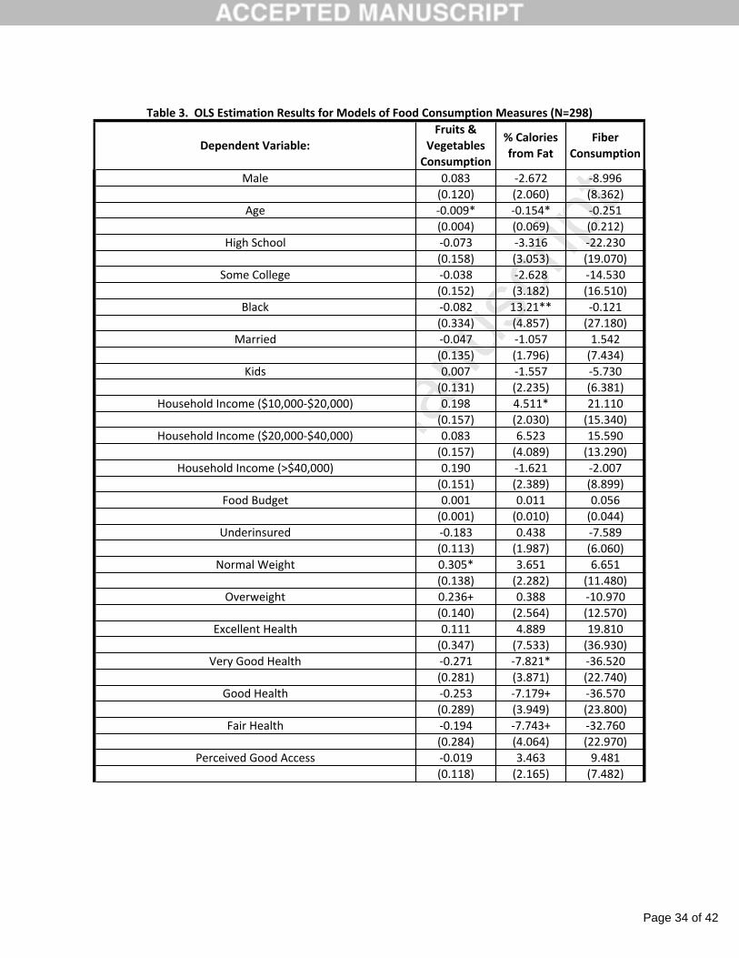
Estimation results and heteroskedasticity robust standard errors are displayed in Table 3.

Only a few socio-cultural and financial characteristics display statistically significant estimated

relationships with dietary intake. This is likely due to the homogenous low-income, minority

composition of the sample. Older individuals tended to consume fewer calories from fat and

fewer fruits and vegetables. Lower income and African American respondents consumed a

higher percentage of calories from fat. Normal weight respondents consumed a higher

proportion of fat (compared to fat consumption among obese respondents), but they also

consumed more fruits and vegetables.

Individual nutrition-related perceptions and behaviors are important correlates of dietary

intake. Individuals who perceived the local supply of grocery stores as adequate tended to

consume more fats whereas more frequent home meal preparation was related to more fruit,

vegetable and fiber consumption.

Page 16 of 42

Accep

ted

Man

uscr

ipt

16

Respondents whose social network was primarily composed of neighborhood residents

consumed a higher percentage of calories from fat. This may be reflective of cultural norms

within the neighborhood. However, individuals whose social network members exercised on a

regular basis ate more fruits and vegetables. These results suggest that the behavioral choices of

geographic peers are related to both more and less healthy decision making.

Variables measuring access to neighborhood food sources were statistically significant

only in the model for fruits and vegetables. For this model, living nearer to a fresh food source

was related to increased fruits and vegetables consumption while living nearer to fast food

restaurants was associated with reduced fruits and vegetables consumption.

The relationships with proximity to food sources would be more meaningful if proximity

was also related to utilization of the food source. Although we were unable to assess this for fast

food restaurants and pantries, we did collect data regarding where participants shopped for

groceries. Grocery shopping behavior was assessed by asking participants for the location of the

grocery store they went to for major grocery shopping trips and the store they went to most often

for smaller trips in between the major grocery trips. This data was only available for 256 of the

study respondents. Sixty-four percent reported shopping at neighborhood fresh food sources. We

estimated a logistic regression model with use of neighborhood fresh food sources for either

major or smaller trips as the dependent variable and proximity to neighborhood fresh food

sources as the key independent variable. Estimation results are presented in Table 4. Proximity to

the neighborhood fresh food sources was the largest determinant of shopping at a neighborhood

fresh food source.

4.2 Geographic Peer Effects in Dietary Intake

Page 17 of 42

Accep

ted

Man

uscr

ipt

17

Next we examined the full spatial lag model indicated in (2). The robust Lagrange

Multiplier tests (Florax, Folmer et al. 2003) indicated that the spatial lag model was the

appropriate model for both fruits and vegetables (LM lag statistic=9.9 vs LM error statistic=6.3)

and fat (LM lag statistic=7.1 vs LM error statistic=6.3); however, the results were inconclusive

for the fiber model (LM lag statistic=0.004 vs LM error statistic=0.006). We based our primary

analysis on a weights matrix for the “8 nearest neighbors” of each individual. Each of the 8

nearest study participants was weighted by inverse straight-line distance, and the W matrix was

row-standardized. All study participants had at least one neighbor within 1/3 of a mile and the

farthest neighbor considered in the analysis was less than 1 mile away. The median distance

between neighbors was 0.11 miles. Inverse distance weighting of neighbors allowed for the

nearest neighbors to have the greatest influence as suggested by Tobler’s first law of geography

(Tobler 1970). Results are robust to alternative specifications of the spatial weights matrix (i.e. 6

nearest neighbors, 10 nearest neighbors and equal weighting of all nearest neighbors).

The estimation results for the spatial lag model and heteroskedasticity robust standard

errors are displayed in Table 5. The coefficient on the average of geographic peers' dietary

intake, ρ, is statistically significant only in the fruits and vegetables model: fruits and vegetables

consumption of geographic peers is positively associated with an individual’s fruits and

vegetables consumption.

The relationships between education, financial, socio-cultural, and social and physical

environment characteristics remain unchanged with only a few exceptions: age is no longer

significant for any outcome, while those with a higher food budget are slightly more likely to

consume a higher percentage of calories from fat and fiber. Also, the correlation between home

food preparation and dietary intake is more pronounced in the spatial models: compared to the

Page 18 of 42

Accep

ted

Man

uscr

ipt

18

reference group who do not cook at home, respondents who cook 1-5 meals at home consume

over a half serving more fruits and vegetables in their diet while those who cook 20 or more

meals at home consume slightly over one additional serving of fruits and vegetables per day (in

comparison to the reference group who do not cook at home). However, while cooking at home

is related to a more healthy diet in terms of fruits and vegetables consumption, the opposite

appears true when considering the percent of calories consumed from fat: more meals prepared at

home is related to a higher percentage of calories from fat.

Both the OLS and spatial lag models find that respondents living nearer to fast food

restaurants incorporate fewer fruits and vegetables into their diet. However, only the OLS

estimation indicates that living closer to fresh food sources is associated with increased in fruits

and vegetables consumption.

4.3 Identification Checks for Geographic Peer Effects

Thus far we have assumed the ρWc term is capturing geographic peer effects in food

consumption. If geographic proximity is a proxy for social influence we expect that the influence

of a respondent’s eight closest neighbors will be greater than the next closest group of eight

neighbors. To evaluate this we compared the fruits and vegetables model (with a weight matrix

of nearest neighbors 1 through 8) to an alternative specification using the same spatial model but

replacing the original weight matrix with a weight matrix containing the next set of eight

neighbors (nearest neighbors 9 through 16). The coefficient of the peer effects term, , in the

alternative specification is insignificant.2

Another concern with the estimated geographic peer effects may be characterized as an

endogeneity issue. While we have referred to the estimated coefficient for the spatially weighted

2 Results available from the authors upon request.

Page 19 of 42

Accep

ted

Man

uscr

ipt

19

fruits and vegetables consumption of geographic peers as a “peer effect” and the model defined

in (2) satisfies the identification criteria for peer effects (Lee 2007; Bramoulle, Djebbari et al.

2009), the causal mechanism for the relationship is unresolved. Of particular concern is the

possibility that the geographic peer effect is being driven by an omitted spatially dependent

variable. This concern is similar to recent critiques regarding the proper causal interpretation of

spatially lagged explanatory variables (Corrado and Fingleton 2012; Partridge, Boarnet et al.

2012). To investigate this possibility, we use instrumental variables to better understand the

nature of the mechanism through which fruits and vegetables consumption of geographic peers is

related to individual fruits and vegetables consumption.

For instruments, we are interested in variables related to fruits and vegetables

consumption of geographic peers, but not related to the individual’s specific fruits and vegetables

consumption. The spatial lag of the geographic peers’ education, financial, socio-cultural, and

social and physical environment characteristics satisfy this condition. Neighbors’ education,

financial, and socio-cultural characteristics (e.g. income, race/ethnicity, education) should not

influence the individual’s own dietary intake unless social influences are at work. The same

argument applies to neighbors' social network measures. The access measures of neighbors may

influence individuals' own dietary intake without social influence if the shared food environment

or some other omitted variable that similarly varies over space (e.g. commercial development,

access to retail, etc.) is responsible for the observed geographic peer effects. As a further test of

the validity of the instruments, we have included them as independent variables in the fruits and

vegetables model and the estimated coefficients were not significant (F-statistic=1.28, p=.1623).

Further the spatial lag of geographic peers’ demographic, network and access variables were

significantly related to the average fruits and vegetables consumption of the peers. In what

Page 20 of 42

Accep

ted

Man

uscr

ipt

20

follows, we use 3 sets of instruments: (1) the full set of spatially lagged education, financial,

socio-cultural, and social and physical environment characteristics variables (F-statistic=10.18,

p=0.000); (2) only the spatially lagged education, financial, socio-cultural, and social network

variables (F-statistic=9.58, p=0.000); and (3) only the spatially lagged physical environment

(access) variables (F-statistic=3.80, p=0.000).

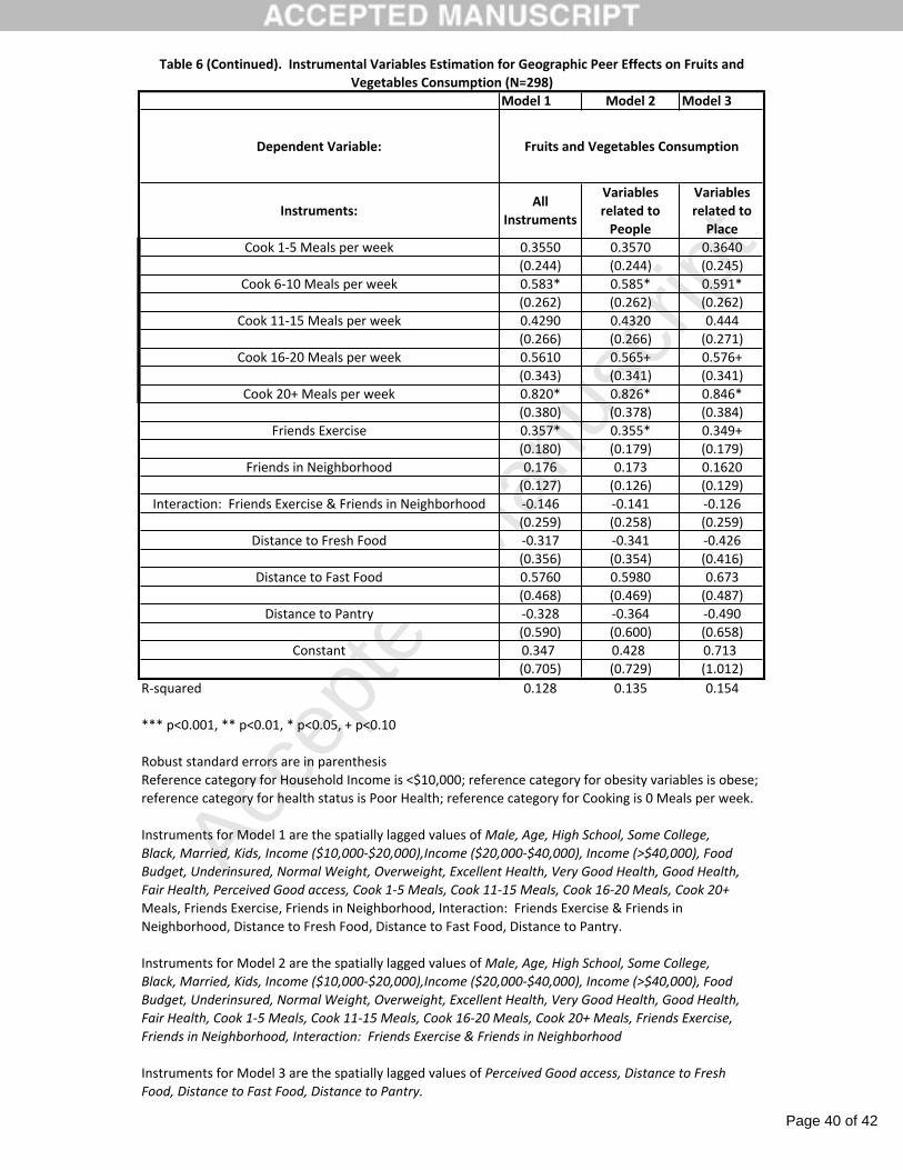
Table 6 presents the results for the fruits and vegetables model where the geographic peer

term (Wc) is instrumented in each of the 3 different ways. First, we observed that the

instrumented Wc term is statistically significant in Model 1 (when the full set of instruments was

used) and Model 2 (when the spatially lagged characteristics of the people were used as

instruments), but not in Model 3 (when the spatially lagged characteristics of the place were used

as instruments).

The estimated results for Models 1 through 3 suggest geographic peers, or some

characteristic of people in the neighborhood, is driving the relationship between geographic

peers’ nutrition and individual nutrition behavior; however, it can be argued, that the results do

not conclusively point to a social mechanism. First, the instruments for Model 3 (those based on

spatially lagged characteristics of the place) are weaker than the instruments for Models 1 and 2.

One might argue that this is precisely because the geographic peer effects are less related to

physical attributes of the environment, but there is also the possibility that we are missing some

important aspect of the environment that would make a stronger instrument. Second, the peer

effects observed in Model 2 (those based upon spatially lagged characteristics of the people) may

be related to geographic sorting: individuals choose their housing location based on shared

interests and characteristics. However, this is unlikely in our sample for a number of reasons.

The sorting hypothesis would require individuals to sort on a very small scale. Usually we

Page 21 of 42

Accep

ted

Man

uscr

ipt

21

consider individuals to sort into neighborhoods, areas of a city, school districts or subdivisions.

If the observed geographic peer effects were a result of sorting, it would require sorting on a

much finer geographic scale—sorting at the block level within a neighborhood. Also, it is

unlikely that this very low-income sample has the means to freely choose their housing location.

The last potential mechanism driving the geographic peer effects is actual social interactions

within the neighborhood among the geographic peers.

These three competing explanations for the IV results reported in Models 1-3 are related

to the critique of Gibbons & Overman (Gibbons and Overman 2012): the crucial assumption

underlying the ability to causally identify endogenous peer effects relies on knowing the proper

specification of the spatial weights matrix. If we know with certainty that the spatial weights

matrix, W, represents true social interactions, then the causal role of geographic peers supported

by Models 1-3 is valid. In the absence of this definitive knowledge of spatially-based social

networks, more experimental approaches that depend upon exploiting variation within the

sample have been advocated (Gibbons and Overman 2012). Next, we use additional information

about the neighborhood environment to exploit such variation.

We do not observe the extent to which geographic peers interact, but we do have data

regarding sociability of the neighborhood. In the first wave of data collection in the

neighborhood, we obtained a spatially weighted sample of 1412 individuals. Each of these

individuals provided answers to two questions pertaining to geographic peer interactions: (1) the

number of people outside of their household that they talk to on a daily basis when they are at

their home and (2) whether they feel comfortable asking someone on the sidewalk for help

carrying something to their home. The crucial element of these survey questions is that they

gauged social interaction behavior near the home—the exact element of social behavior that

Page 22 of 42

Accep

ted

Man

uscr

ipt

22

would generate geographic peer effects. The answers to these questions were categorical and we

used them to create two binary variables: Talk is an indicator variable for individuals who talked

with 6 or more non-household members on days that they were home3; and help is an indicator

variable for individuals who were always or sometimes willing to ask a passerby for help

carrying something to their home. For each of the current study participants (the N=298

sample), we calculated the percentage of first wave respondents (the N=1412 sample) within 400

meters of their home for which talk took on a value of 1 (pct_talk) and the percentage of

respondents within 400 meters of their home for which help took on a value of 1 (pct_help).

Pct_talk and pct_help were then normalized for our sample of 298 observations, and we

stratified the sample based on the normalized values. Estimation results based on the stratified

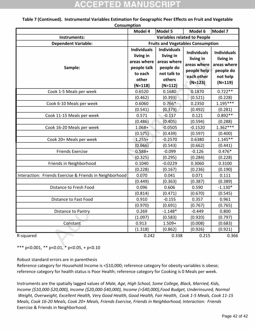
samples are presented in Table 7. Model 4 reports the instrumental variables regression using

the “people” instruments (spatially lagged demographic and network characteristics) when

pct_talk is more than 0.25 standard deviations greater than the average, and Model 5 reports the

same regression results for the sub-sample in which pct_talk is more than 0.25 standard

deviations less than the average. Likewise, Model 5 is based on the sample for pct_help more

than 0.25 standard deviations above the average, and Model 6 is based on the sample for

pct_help more than 0.25 standard deviations below the average. Geographic peer effects are

statistically significant only for individuals living in neighborhoods where neighbors reported

talking to others (Model 4) and felt able to ask each other for help (Model 6). These results

strongly imply a social mechanism for the estimated relationship between individual and

geographic peer consumption of fruits and vegetables.

5. Discussion and Conclusions

3 Response choices for the question upon which Talk is based were less than 3, 3‐5, 6‐10 or more than 10. We chose 6 as the cut‐point because it was the mid‐point of the possible answer choices.

Page 23 of 42

Accep

ted

Man

uscr

ipt

23

The results highlight the role of social factors in nutrition determinants and point to a

need for comprehensive solutions to improve dietary behavior of low-income individuals.

However, these findings should be considered in light of the limitations of the study. First, the

sample came from a single low-income neighborhood, thus impacting the generalizability and

external validity of study findings to other low income minority neighborhoods. Second, we

have incomplete data on the geographic peer network because network members were restricted

to being in the study’s sample. Additionally, we only have self-report information about the

social network characteristics, and we do not know the degree to which social and geographic

peer networks overlapped in the sample. Third, the distance between study participants and food

sources were calculated using straight-line distance, which often underestimates the actual

distance using the road network. Associations using distance measured along the road network

may differ from those reported here. Fourth, beyond social and environmental factors, individual

attitudes, knowledge and preferences impact dietary intake. The Socio-Ecological model

emphasizes the multitude of factors affecting health behaviors on the intrapersonal,

interpersonal, and community levels (National Cancer Institute 2005). While the current study

takes into account aspects of the social and physical environment (i.e. interpersonal and

community levels), the intrapersonal level is not comprehensively examined. For example,

participants’ knowledge of the importance of a healthful diet, self-efficacy to modify nutritional

behavior, and perceived threats, benefits, and cues for action for adhering to healthful diet

(components of the Health Belief Model) have been found to affect dietary intake and are not

taken into account in the current study (National Cancer Institute 2005; Shaikh, Yaroch et al.

2008). Finally, the measures of dietary intake are derived from a validated instrument developed

by the National Cancer Institute, but the instrument is only viewed as a screener for nutrition

Page 24 of 42

Accep

ted

Man

uscr

ipt

24

factors related to cancer and other health outcomes. A more comprehensive dietary

questionnaire, such as the Food Frequency Questionnaire (Willett and Lenart 1998; Flagg,

Coates et al. 2000) or biochemical markers of food consumption (Day, McKeown et al. 2001)

might have provided a more accurate measure of dietary intake.

The association between proximity to healthy food sources (i.e. fresh food sources and

pantries) and diet was smaller in magnitude and not statistically significant in the spatial models.

However, the estimated magnitude of the association between proximity to fast food and diet

was larger and more statistically significant in the spatial models. This may be because peer

behavior is an important modifier of the relationship between the environment and dietary intake.

Results also suggest that perhaps chain grocery outlets (often the primary focus when

considering access) might need to be considered along with an array of other food sources. Our

measures of healthy food sources included a variety of different food sources commonly found in

low-income communities: charitable pantries, chain grocers, and small, non-traditional food

sources. Further, we found that proximity to the nearest fresh food source was positively related

to whether or not participants listed a neighborhood food source as their primary or secondary

grocery store. However, further work is needed to elucidate the causal nature of this correlative

relationship since individuals sort into neighborhoods, and likewise commercial and non-profit

food sources are purposefully located near prospective consumers.

Our findings pertaining to the role of proximity and social influences in determining

dietary intake emphasize the need for policymakers and intervention designers to acknowledge

the reciprocal relationship between people and place. Social marketing and education campaigns

can be designed to address dietary norms, the types of foods provided by non-profit agencies,

and peer behaviors. Our results suggest that these initiatives will be most effective if they are

Page 25 of 42

Accep

ted

Man

uscr

ipt

25

implemented to target specific geographic locations on multiple fronts to effectively address both

the demand and supply of healthy foods.

Finally, study results highlight the potential role of geographic peer effects in individual

nutrition behavior which is consistent with previous research finding a relationship between

nutrition intake and social ties among African Americans (Yeh, Ickes et al. 2008; Zhylyevskyy,

Jensen et al. 2012). While we modeled social influence as peer effects, our work was unable to

distinguish direct peer-to-peer influences from social norms. Future studies should re-examine

the endogenous relationship between peers' nutritional behavior using well-defined social

network data (rather than geographic proximity). Behavioral economists might additionally

focus on understanding the external validity of peer effects on nutritional behavior across

different preferences for time and risk—factors which have been shown to impact obesity related

outcomes/behaviors (Lusk and Coble 2005; Anderson and Mellor 2008; Richards and Hamilton

2012). Additionally, future behavioral interventions may be designed to produce an exogenous

change in nutrition behavior that leverages and facilitates measurement of social multiplier

effects in peers’ nutrition outcomes.

Funding: This study was funded by the National Science Foundation (NSF/SES-0827350).

Page 26 of 42

Accep

ted

Man

uscr

ipt

26

References

Health Impact Assessment (HIA). The Determinants of Health. W. H. O. (WHO). Akerlof, G. A. (1997). "Social distance and social decisions." Econometrica: Journal of the Econometric

Society: 1005‐1027. An, R. and R. Sturm (2012). "School and Residential Neighborhood Food Environment and Diet Among

California Youth." American Journal of Preventive Medicine 42(2): 129‐135. Anderson, L. R. and J. M. Mellor (2008). "Predicting health behaviors with an experimental measure of

risk preference." Journal of Health Economics 27(5): 1260‐1274. Anselin, L. (1988). Spatial Econometrics: Methods and Models, Kluwer Academic Publishers. Azar, O. H. (2004). "What sustains social norms and how they evolve?: The case of tipping." Journal of

Economic Behavior & Organization 54(1): 49‐64. Block, G., B. Patterson, et al. (1992). "Fruit, vegetables, and cancer prevention: A review of the

epidemiological evidence." Nutrition and Cancer 18(1): 1‐29. Bramoulle, Y., H. Djebbari, et al. (2009). "Identification of peer effects through social networks." Journal

of Econometrics 150(1): 41‐55. Burdette, H. L. and R. C. Whitaker (2004). "Neighborhood playgrounds, fast food restaurants, and crime:

relationships to overweight in low‐income preschool children." Preventive Medicine 38(1): 57‐63.

Chen, S., R. J. G. M. Florax, et al. (2010). "Obesity and Access to Chain Grocers." Economic Geography 86(4): 431‐452.

Chiteji, N. (2010). "Time‐preference, Non‐cognitive Skills and Well‐being across the Life Course: Do Non‐cognitive Skills Encourage Healthy Behavior?" The American Economic Review 100(2): 200.

Christakis, N. A. and J. H. Fowler (2007). "The Spread of Obesity in a Large Social Network over 32 Years." New England Journal of Medicine 357(4): 370‐379.

Cohen‐Cole, E. and J. M. Fletcher (2008). "Detecting implausible social network effects in acne, height, and headaches: longitudinal analysis." BMJ: British Medical Journal 337.

Cohen‐Cole, E. and J. M. Fletcher (2008). "Is obesity contagious? Social networks vs. environmental factors in the obesity epidemic." Journal of Health Economics 27(5): 1382‐1387.

Corrado, L. and B. Fingleton (2012). "Where is the economics in spatial econometrics? ." Journal of Regional Science 52(2): 210‐239.

Corrado, L. and B. Fingleton (2012). "WHERE IS THE ECONOMICS IN SPATIAL ECONOMETRICS?*." Journal of Regional Science 52(2): 210‐239.

Davezies, L., X. D'Haultfoeuille, et al. (2009). "Identification of peer effects using group size variation." Econometrics Journal 12(3): 397‐413.

Day, N. E., N. McKeown, et al. (2001). "Epidemiological assessment of diet: a comparison of a 7‐day diary with a food frequency questionnaire using urinary markers of nitrogen, potassium and sodium." International Journal of Epidemiology 30(2): 309‐317.

Dietz, R. D. (2002). "The estimation of neighborhood effects in the social sciences: An interdisciplinary approach." Social Science Research 31(4): 539‐575.

Do, D. P., T. Dubowitz, et al. (2007). "Neighborhood context and ethnicity differences in body mass index: a multilevel analysis using the NHANES III survey (1988‚Äì1994)." Economics & Human Biology 5(2): 179‐203.

Durlauf, S. N. (2004). "Neighborhood effects." Handbook of regional and urban economics 4: 2173‐2242. Durlauf, S. N. and Y. M. Ioannides (2010). "Social interactions." Annu. Rev. Econ. 2(1): 451‐478.

Page 27 of 42

Accep

ted

Man

uscr

ipt

27

Eisenberg, D. and B. C. Quinn (2006). "Estimating the Effect of Smoking Cessation on Weight Gain: An Instrumental Variable Approach." Health Services Research 41(6): 2255‐2266.

Elster, J. (1989). "Social norms and economic theory." The Journal of Economic Perspectives 3(4): 99‐117.

Finkelstein, E. A., K. L. Strombotne, et al. (2010). "The Costs of Obesity and Implications for Policymakers." Choices 25(3).

Flagg, E. W., R. J. Coates, et al. (2000). "Validation of the American Cancer Society Cancer Prevention Study II Nutrition Survey Cohort Food Frequency Questionnaire." Epidemiology 11(4).

Florax, R. J. G. M., H. Folmer, et al. (2003). "Specification searches in spatial econometrics: the relevance of Hendry‚Äôs methodology." Regional Science and Urban Economics 33(5): 557‐579.

Getz, G. S. and C. A. Reardon (2007). "Nutrition and Cardiovascular Disease." Arteriosclerosis, Thrombosis, and Vascular Biology 27(12): 2499‐2506.

Gibbons, S. and H. G. Overman (2012). "MOSTLY POINTLESS SPATIAL ECONOMETRICS?*." Journal of Regional Science 52(2): 172‐191.

Glanz, K., M. Basil, et al. (1998). "Why Americans Eat What They Do: Taste, Nutrition, Cost, Convenience, and Weight Control Concerns as Influences on Food Consumption." Journal of the American Dietetic Association 98(10): 1118‐1126.

Grossman, M. (1972). "On the concept of health capital and the demand for health." The journal of political economy 80(2): 223‐255.

Grossman, M. (2000). "The human capital model." Handbook of health economics 1: 347‐408. Habyarimana, J., M. Humphreys, et al. (2007). "Why Does Ethnic Diversity Undermine Public Goods

Provision?" American Political Science Review 101(04): 709‐725. Hill, J. O. (2006). "Understanding and Addressing the Epidemic of Obesity: An Energy Balance

Perspective." Endocrine Reviews 27(7): 750‐761. Hung, H.‐C., K. J. Joshipura, et al. (2004). "Fruit and vegetable intake and risk of major chronic disease."

Journal of the National Cancer Institute 96(21): 1577‐1584. Huston, S. J. and M. S. Finke (2003). "Diet choice and the role of time preference." Journal of Consumer

Affairs 37(1): 143‐160. Ichiro, K., K. Daniel, et al. (2004). "Commentary: Reconciling the three accounts of social capital."

International Journal of Epidemiology 33(4): 682‐690. Ioannides, Y. (2012). From Neighborhoods to Nations‐The Economics of Social Interactions, Princeton

University Press. Jung, S., D. Spiegelman, et al. (2013). "Fruit and Vegetable intake and risk of Breast cancer by Hormone

receptor Status." Journal of the National Cancer Institute 105(3): 219‐236. Kallbekken, S., H. Westskog, et al. (2010). "Appeals to social norms as policy instruments to address

consumption externalities." The Journal of Socio‐Economics 39(4): 447‐454. Keane, C. R., J. M. Lafky, et al. (2012). "Altruism, reciprocity and health: A social experiment in restaurant

choice." Food Policy 37(2): 143‐150. Lee, L. (2007). "Identification and estimation of econometric models with group interactions, contextual

factors and fixed effects." Journal of Econometrics 140(2): 333‐374. LeSage, J. (2012). "Econometrics Toolbox." Retrieved March 25, 2012, from http://www.spatial‐

econometrics.com/. LeSage, J. and R. K. Pace (2009). Introduction to Spatial Econometrics, CRC Press/Taylor & Francis Group. Lopez‐Perez, R. (2009). "Followers and leaders: Reciprocity, social norms and group behavior." The

Journal of Socio‐Economics 38(4): 557‐567. Lusk, J. L. and K. H. Coble (2005). "Risk perceptions, risk preference, and acceptance of risky food."

American Journal of Agricultural Economics 87(2): 393‐405.

Page 28 of 42

Accep

ted

Man

uscr

ipt

28

Lyons, R. (2011). "The spread of evidence‐poor medicine via flawed social‐network analysis." Statistics, Politics, and Policy 2(1).

Maddock, J. (2004). "The relationship between obesity and the prevalence of fast food restaurants: state‐level analysis." American journal of health promotion : AJHP 19(2): 137‐143.

Manski, C. F. (1993). "Identification of endogenous social effects: The reflection problem." The review of economic studies 60(3): 531‐542.

Moore, K., A. V. D. Roux, et al. (2013). "Home and work neighbourhood environments in relation to body mass index: the Multi‐Ethnic Study of Atherosclerosis (MESA)." Journal of Epidemiology and Community Health.

Moore, L. V., A. V. Diez Roux, et al. (2008). "Associations of the Local Food Environment with Diet Quality‚ÄîA Comparison of Assessments based on Surveys and Geographic Information Systems." American Journal of Epidemiology 167(8): 917‐924.

Morland, K., A. V. Diez Roux, et al. (2006). "Supermarkets, Other Food Stores, and Obesity: The Atherosclerosis Risk in Communities Study." American Journal of Preventive Medicine 30(4): 333‐339.

Morland, K. B. and K. R. Evenson (2009). "Obesity prevalence and the local food environment." Health & Place 15(2): 491‐495.

Naik, N. Y. and M. J. Moore (1996). "Habit Formation and Intertemporal Substitution in Individual Food Consumption." The Review of Economics and Statistics 78(2): 321‐328.

National Cancer Institute (2005). A Guide For Health Promotion Practice. Theory at A Glance. Washington, DC, National Institutes of Health.

Noel, H. and B. Nyhan (2011). "The ‚Äúunfriending‚Äù problem: The consequences of homophily in friendship retention for causal estimates of social influence." Social Networks 33(3): 211‐218.

Partridge, M. D., M. Boarnet, et al. (2012). "Introduction: Whither Spatial Econometrics?" Journal of Regional Science 52(2): 167‐171.

Patrick, H. and T. A. Nicklas (2005). "A Review of Family and Social Determinants of Children‚Äôs Eating Patterns and Diet Quality." Journal of the American College of Nutrition 24(2): 83‐92.

Richards, T. J. and S. F. Hamilton (2012). "Obesity and Hyperbolic Discounting: An Experimental Analysis." Journal of Agricultural and Resource Economics 37(2): 181.

Sainsbury, P. (2008). "Commentary: Understanding social network analysis." BMJ 337. Satija, A. and F. B. Hu (2012). "Cardiovascular Benefits of Dietary Fiber." Current Atherosclerosis Reports

14(6): 505‐514. Shaikh, A. R., A. L. Yaroch, et al. (2008). "Psychosocial predictors of fruit and vegetable consumption in

adults: A review of the literature." American Journal of Preventive Medicine 34(6): 535‐543. e511.

Shalizi, C. R. and A. C. Thomas (2011). "Homophily and contagion are generically confounded in observational social network studies." Sociological Methods & Research 40(2): 211‐239.

Simmons, D., A. McKenzie, et al. (2005). "Choice and availability of takeaway and restaurant food is not related to the prevalence of adult obesity in rural communities in Australia." Int J Obes Relat Metab Disord 29(6): 703‐710.

Starr, M. A. (2009). "The social economics of ethical consumption: Theoretical considerations and empirical evidence." The Journal of Socio‐Economics 38(6): 916‐925.

Threapleton, D. E., D. C. Greenwood, et al. (2013). "Dietary Fiber Intake and Risk of First Stroke A Systematic Review and Meta‐Analysis." Stroke 44(5): 1360‐1368.

Tobler, W. R. (1970). "A computer movie simulating urban growth in the Detroit region." Economic Geography 46: 234‐240.

Turrell, G. (1996). "Structural, material and economic influences on the food‐purchasing choices of socioeconomic groups." Australian and New Zealand Journal of Public Health 20(6): 611‐617.

Page 29 of 42

Accep

ted

Man

uscr

ipt

29

Turrell, G. and A. M. Kavanagh (2005). "Socio‐economic pathways to diet: modelling the association between socio‐economic position and food purchasing behaviour." Public Health Nutrition 9(3): 8.

US House of Representatives Select Committee on Hunger (1987). Obtaining Food: Shopping constraints on the Poor. Washington, DC, US Government Printing Office.

US House of Representatives Select Committee on Hunger (1992). Urban Grocery Gap. Washington, DC, US Government Printing Office: 20‐21.

Ver Ploeg, M., V. Breneman, et al. (2009). Access to Affordable and Nutritious Food‐‐Measuring and Understanding Food Desserts and Their Consequences: Report to Congress. E. R. Service: 160.

Viswanath, K. and K. Bond (2007). "Social Determinants and Nutrition: Reflections on the Role of Communication." Journal of Nutrition Education and Behavior 39(2, Supplement): S20‐S24.

Viswanath, K. W. R. J. J. R. (2006). "Social Capital and Health: Civic Engagement, Community Size, and Recall of Health Messages." American Journal of Public Health 96(8): 1456‐1461.

Wada, R. and E. Tekin (2010). "Body composition and wages." Economics & Human Biology 8(2): 242‐254.

Walker, R. E., C. R. Keane, et al. (2010). "Disparities and access to healthy food in the United States: a review of food deserts literature." Health & Place 16(5): 876‐884.

Wang, L., J. E. Manson, et al. (2012). "Fruit and vegetable intake and the risk of hypertension in middle‐aged and older women." American journal of hypertension 25(2): 180‐189.

Wang, M. C., S. Kim, et al. (2007). "Socioeconomic and food‐related physical characteristics of the neighbourhood environment are associated with body mass index." Journal of Epidemiology and Community Health 61(6): 491‐498.

Wen, M. and T. N. Maloney (2013). "Neighborhood socioeconomic status and BMI differences by immigrant and legal status: Evidence from Utah." Economics & Human Biology.

Willett, W. and E. Lenart, Eds. (1998). Reproducibility and validity of food‐frequency questionnaires. Nutritional Epidemiology. Oxford, United Kingdom, Oxford University Press.

World Health Organization. (2013). "Obesity and overweight fact sheet." Retrieved March 17, 2014, 2014, from http://www.who.int/mediacentre/factsheets/fs311/en/.

Yeh, M.‐C., S. B. Ickes, et al. (2008). "Understanding barriers and facilitators of fruit and vegetable consumption among a diverse multi‐ethnic population in the USA." Health Promotion International 23(1): 42‐51.

Zhen, C., M. K. Wohlgenant, et al. (2011). "Habit Formation and Demand for Sugar‐Sweetened Beverages." American Journal of Agricultural Economics 93(1): 175‐193.

Zhylyevskyy, O., H. H. Jensen, et al. (2012). "Effects of Family, Friends, and Relative Prices on Fruit and Vegetable Consumption by African Americans." Southern Economic Journal.

Page 30 of 42

Accep

ted

Man

uscr

ipt

30

Highlights

We analyze neighborhood correlates of nutrition in a low‐income, neighborhood.

Access to food sources and social influence were found to impact dietary intake.

Social influence is strongest where neighbors report more neighborhood interaction.

Neighborhood social environment is important for nutrition choices.

Page 31 of 42

Accep

ted

Man

uscr

ipt

")

")

")

")")

")

")")

")

")")

")

")

") ")

")")

")

")

")

" "

"""

"""

"""

""

"

""""

"

"

""""

"

"

" "

"

" ""

"

"

"""

"

"

""

"

")

")")

")

")

")

")

")

")

")

")

")

")

")

")

")

")")")")

")

")

")

")

")

")

")

")

")

")

")

")

")

")

")

")")

")

")

")

")

")

")

")")

")

")

")

")

")

")

!(

!(

!(

!(

!(

!(

!(

!(

!(!( !(!(!(!( !(

!(!(!(!(!(!(!( !(!( !(!(!( !(!(!( !( !( !(!(!( !(!( !(!( !(!( !( !(!(!( !(!( !(!( !(!(!(!( !( !(!( !(!( !( !(!( !(!(!( !( !(!( !( !(!( !(!( !( !(!( !(!(!(!( !(!( !(!(!(!( !(!(!(!(!(

!(!( !(!(!( !(!(!( !(

!(!( !( !(!( !(!( !(!(!(!( !(

!(!(!(!(

!( !(!( !(!(!( !(!( !(!( !( !(!(

!( !(!(!(!(

!( !(!(!(!(

!(!(!(!( !(!( !( !(!(!( !( !(!( !(!(!(!( !(!(!( !(!( !(!( !(!( !(!( !(!(!(!( !( !(!(!( !( !(!(!(!(!( !(!( !( !( !(!(!( !(!( !( !(!( !(!( !(!(!( !(!(

!( !(!(!(!(!( !( !(!(!( !(!(!(!( !( !(!(!(!( !(!(!(!( !(!(!(

!(!(!( !(!(!(!(!(

!(

!(!(!(

!(!(

!(!(

!(!(

!(

!( !(!(!(!( !(

!(!(

!( !(!( !(!(!( !(!(

!(!(!(!(

!(!(!(!(!( !(!( !(!( !(!( !(!(

!( !( !(!(!(!(!( !(!( !(!( !(!(!(!( !(!( !(!( !( !(!(!( !(!(

!(!( !(!( !(!(!( !(!(!( !(!( !( !(!(!(!(

!(!(!(!(

!(!(!( !(!(!(!( !(!(!(!(!(!( !(!( !(

!(

!( !(!(!( !(!( !(!(!(!( !(!( !(!( !(!(!( !( !(!( !(!( !(!(!( !(!(!(!(!(

!(!(

!(!(

!(!(

!(

!(!(!(!(!(!(!(!(!(!(

!(!(!(!(!(!(

!(!(!(!(!(!(!(!(

!(!(!(!(!(!(!(!(!(!(!(!(!(!(!(!(!(!(!(!(!(!(!(!(!(!(!(!(!(!(

!(

!(

!(!(!(

!(

!(!(

!(

!(

!(!(

!(

!(

!(

!(

!(

!(

!(

!(

!(

!(

!(!(

!(

!(!(!(

!(!(

!(

!(

!(

!(!(!(!(!(!(!(!(!(!(!(!(!(!(!(!(!(

!(!(

!(

!(

!(

!(!(!(

!(

Legend!( Survey Participants

" Fast Food Source

") Fresh and Fast food Source

") Fresh Food Source

") Charitable Food Pantries

Highways

Fair Park Boundary

N0 0.55 1.10.275 Miles

Figure 1. Location of Survey Participants and Food Sources

Table

Page 32 of 42

Accep

ted

Man

uscr

ipt

Table&1.&&Variable&DeffinitionsVariable DescriptionDependent&VariablesFat Variance*adjusted*percent*calories*obtained*from*fat

Fruit*&*Vegetables*(no*fries)Variance*adjusted*fruit*and*vegetable*intake*excluding*fried*potatoes*(pyramid*servings)

Fiber Variance*adjusted*grams*of*fiber*consumed*Educational&AttainmentLess*than*High*School Respondent*did*not*complete*a*college*degree*or*equivalentHigh*School Respondent*has*a*high*school*degree*or*equivalentSome*College Respondent*has*completed*at*least*some*college*coursesSocio:Cultural&CharacteristicsMale Respondent*is*maleAge Respondent's*ageBlack Respondent*is*African*AmericanMarried Respondent*is*married*or*living*with*a*partnerKids Respondent's*household*includes*kids*less*than*18*years*of*ageUnderinsured Respondent*has*inadquate*health*insuranceNormal*Weight BMI*is*less*than*25*kg/m^2Overweight BMI*is*25U29.9*kg/m^2Obese BMI*is*>29.9*kg/m^2Excellent*Health SelfUreported*health*is*excellentVery*Good*Health SelfUreported*health*is*very*goodGood*Health SelfUreported*health*is*goodFair*Health SelfUreported*health*is*fairPoor*Health SelfUreported*health*is*poorCharacteristics&of&the&Social&EnvironmentFriends*Exercise Many*or*all*close*friends*and*family*exercise*on*a*regular*basisFriends*in*Neighborhood Many*or*all*close*friends*and*family*live*in*the*neighborhoodFriends*Exercise*&*in*Neighborhood

Interaction:**Many*or*all*close*friends*and*family*exercise*and*live*in*neighborhood

Characteristics&of&the&Physical&EnvironmentDistance*to*Fresh*Food Miles*from*home*to*the*nearest*neighborhood*fresh*food*sourceDistance*to*Fast*Food Miles*from*home*to*the*nearest*fast*food*sourceDistance*to*Pantry Miles*from*home*to*the*nearest*charitable*food*pantryPerceived*Good*Access Agrees*or*strongly*agrees*neighborhood*grocery*stores*are*adequateCharacteristics&of&health&input&pricesIncome*(<$10,000) Household*income*is*less*than*$10,000Income*($10,000U$20,000) Household*income*is*between*$10,000*and*$20,000Income*($20,000U$40,000) Household*income*is*between*$20,000*and*$40,000Income*(>$40,000) Household*income*is*greater*than*$40,000Food*Budget Monthly*food*expenditures*divided*by*household*sizeDon't*Cook Respondent*typically*prepares*no*meals*at*homeCook*1U5*Meals Respondent*typically*prepares*1U5*meals*per*week*at*homeCook*6U10*Meals Respondent*typically*prepares*6U10*meals*per*week*at*homeCook*11U15*Meals Respondent*typically*prepares*11U15*meals*per*week*at*homeCook*16U20*Meals Respondent*typically*prepares*16U20*meals*per*week*at*homeCook*20+*Meals Respondent*typically*prepares*more*than*20*meals*per*week*at*home

Page 33 of 42

Accep

ted

Man

uscr

ipt

Table&2.&&Summary&Statistics&for&Variables&Included&in&the&Regression&ModelsVariable Mean Standard&Deviation Minimum Maximum

Dependent&VariablesFat 38.60 13.11 16.88 158.36

Fat+males 37.70 6.32 30.58 66.76Fat+females 39.27 16.41 16.88 158.36

Fruit&&&Vegetables&(no&fries) 3.49 3.58 0.00 22.33Fruit8&8Vegetables8(no8fries)+males 3.71 3.42 0.00 20.05Fruit8&8Vegetables8(no8fries)+females 3.33 3.70 0.00 22.33

Fiber 26.11 49.78 6.49 660.75Fiber+males 24.24 20.56 9.05 132.84Fiber+females 27.49 63.30 6.49 660.75

Educational&AttainmentLess&than&High&School 0.23 0.42 0 1

High&School 0.40 0.49 0 1Some&College 0.37 0.48 0 1

SocioICultural&CharacteristicsMale 0.43 0.50 0 1Age 44.53 14.09 18 88Black 0.93 0.26 0 1

Married 0.25 0.43 0 1Kids 0.47 0.50 0 1

Underinsured 0.41 0.49 0 1Normal&Weight 0.30 0.46 0 1Overweight 0.26 0.44 0 1

Obese 0.44 0.50 0 1Excellent&Health 0.10 0.30 0 1Very&Good&Health 0.25 0.43 0 1

Good&Health 0.36 0.48 0 1Fair&Health 0.24 0.43 0 1Poor&Health 0.05 0.21 0 1

Characteristics&of&the&Social&EnvironmentFriends&Exercise 0.29 0.46 0 1

Friends&in&Neighborhood 0.44 0.50 0 1Interaction:&&Friends&Exercise&&&Friends&in&Neighborhood 0.14 0.35 0 1

Characteristics&of&the&Physical&EnvironmentPerceived&Good&Access 0.37 0.48 0 1

Distance&to&Fresh&Food&(miles) 0.24 0.15 0 0.84Distance&to&Fast&Food&(miles) 0.18 0.11 0 0.55Distance&to&Pantry&(miles) 0.17 0.12 0 0.62

Characteristics&of&health&input&pricesHousehold&Income&(<$10,000) 0.49 0.50 0 1

Household&Income&($10,000I$20,000) 0.24 0.43 0 1Household&Income&($20,000I$40,000) 0.19 0.40 0 1

Household&Income&(>$40,000) 0.15 0.35 0 1Food&Budget&($/Month/person) 136.25 117.76 0 800

Don't&Cook 0.07 0.25 0 1Cook&1I5&Meals&per&week 0.55 0.50 0 1Cook&6I10&Meals&per&week 0.17 0.38 0 1Cook&11I15&Meals&per&week 0.09 0.28 0 1Cook&16I20&Meals&per&week 0.06 0.24 0 1Cook&20+&Meals&per&week 0.06 0.24 0 1

Page 34 of 42

Accep

ted

Man

uscr

ipt

Dependent'Variable:Fruits'&'

Vegetables'Consumption

%'Calories'from'Fat

Fiber'Consumption

Male 0.083 )2.672 )8.996(0.120) (2.060) (8.362)

Age )0.009* )0.154* )0.251(0.004) (0.069) (0.212)

High9School )0.073 )3.316 )22.230(0.158) (3.053) (19.070)

Some9College )0.038 )2.628 )14.530(0.152) (3.182) (16.510)

Black )0.082 13.21** )0.121(0.334) (4.857) (27.180)

Married )0.047 )1.057 1.542(0.135) (1.796) (7.434)

Kids 0.007 )1.557 )5.730(0.131) (2.235) (6.381)

Household9Income9($10,000)$20,000) 0.198 4.511* 21.110(0.157) (2.030) (15.340)

Household9Income9($20,000)$40,000) 0.083 6.523 15.590(0.157) (4.089) (13.290)

Household9Income9(>$40,000) 0.190 )1.621 )2.007(0.151) (2.389) (8.899)

Food9Budget 0.001 0.011 0.056(0.001) (0.010) (0.044)

Underinsured )0.183 0.438 )7.589(0.113) (1.987) (6.060)

Normal9Weight 0.305* 3.651 6.651(0.138) (2.282) (11.480)

Overweight 0.236+ 0.388 )10.970(0.140) (2.564) (12.570)

Excellent9Health 0.111 4.889 19.810(0.347) (7.533) (36.930)

Very9Good9Health )0.271 )7.821* )36.520(0.281) (3.871) (22.740)

Good9Health )0.253 )7.179+ )36.570(0.289) (3.949) (23.800)

Fair9Health )0.194 )7.743+ )32.760(0.284) (4.064) (22.970)

Perceived9Good9Access )0.019 3.463 9.481(0.118) (2.165) (7.482)

Table'3.''OLS'Estimation'Results'for'Models'of'Food'Consumption'Measures'(N=298)

Page 35 of 42

Accep

ted

Man

uscr

ipt



%'Calories'from'Fat

Fiber'Consumption

Table'3'(Continued).''OLS'Estimation'Results'for'Models'of'Food'Consumption'Measures'(N=298)

Cook$1&5$Meals$per$week 0.388 3.241 7.973(0.265) (3.320) (12.370)

Cook$6&10$Meals$per$week 0.614* 3.725 9.491(0.281) (3.117) (12.450)


Cook$16&20$Meals$per$week 0.619+ 8.177 58.490(0.355) (6.181) (52.970)

Cook$20+$Meals$per$week 0.917* 14.240 59.570(0.398) (8.754) (40.380)

Friends$Exercise 0.324+ 1.825 3.375(0.182) (2.142) (7.513)

Friends$in$Neighborhood 0.124 5.685* 8.649(0.133) (2.486) (8.723)

Interaction:$$Friends$Exercise$&$Friends$in$Neighborhood &0.069 &5.400 14.750(0.263) (4.290) (25.500)

Distance$to$Fresh$Food &0.734* &4.688 &22.250(0.360) (8.381) (33.180)

Distance$to$Fast$Food 0.948+ &2.048 &6.493(0.487) (8.138) (30.630)

Distance$to$Pantry &0.950 3.629 13.940(0.584) (11.500) (48.680)

Constant 1.751** 31.44*** 57.980(0.653) (8.765) (54.080)

***$p<0.001,$**$p<0.01,$*$p<0.05,$+$p<0.10

Robust$standard$errors$are$in$parenthesisReference$category$for$Household$Income$is$<$10,000;$reference$category$for$obesity$variables$is$obese;$reference$category$for$health$status$is$Poor$Health;$reference$category$for$Cooking$is$0$Meals$per$week.

Page 36 of 42

Accep

ted

Man

uscr

ipt

Dependent'Variable: Individual'shops'at'a'neighborhood'fresh'food'source

Distance)to)Fresh)Food /1.980*(0.899)

Male 0.210(0.290)

Age 0.0274*(0.012)

High)School /0.307(0.378)

Some)College /0.283(0.397)

Black 0.566(0.682)

Married 0.224(0.345)

Kids 0.309(0.318)

Household)Income)($10,000/$20,000) /0.026(0.347)

Household)Income)($20,000/$40,000) /0.016(0.387)

Household)Income)(>$40,000) 0.094(0.428)

Food)Budget 0.000(0.001)

Underinsured 0.135(0.286)

Normal)Weight /0.634+(0.351)

Overweight /0.633+(0.349)

Excellent)Health /0.584(0.867)

Very)Good)Health /0.232(0.803)

Good)Health /0.534(0.791)

Fair)Health /0.563(0.790)

Constant 0.040(1.138)

***)p<0.001,)**)p<0.01,)*)p<0.05,)+)p<0.10

Robust)standard)errors)are)in)parenthesisReference)category)for)Household)Income)is)<$10,000;)reference)category)for)obesity)variables)is)obese;)reference)category)for)health)status)is)Poor)Health.

Table'4.''Logistic'Regression'for'Utilization'of'Neighborhood'Fresh'Food'Sources'(N=256)

Page 37 of 42

Accep

ted

Man

uscr

ipt



%'Calories'from'Fat

Fiber'Consumption

Rho 0.175* 0.079 +0.008(0.084) (0.084) (0.097)

Male 0.111 +2.286 +8.499(0.112) (1.914) (8.435)

Age +0.004 +0.053 +0.031(0.004) (0.071) (0.308)

High;School +0.017 +2.048 +19.975+(0.143) (2.458) (10.826)

Some;College 0.027 +1.424 +12.427(0.151) (2.580) (11.363)

Black 0.255 19.971*** 13.722(0.240) (4.173) (18.035)

Married +0.052 +1.004 1.528(0.134) (2.296) (10.121)

Kids 0.092 0.177 +2.062(0.120) (2.063) (9.052)

Household;Income;($10,000+$20,000) 0.162 4.086+ 20.387*(0.135) (2.307) (10.167)

Household;Income;($20,000+$40,000) 0.083 6.604** 15.789(0.149) (2.557) (11.272)

Household;Income;(>$40,000) 0.195 +1.224 +1.445(0.173) (2.972) (13.098)

Food;Budget 0.001 0.014+ 0.061+(0.001) (0.008) (0.036)

Underinsured +0.155 1.087 +6.295(0.111) (1.895) (8.351)

Normal;Weight 0.379** 5.285* 10.308(0.130) (2.239) (9.816)

Overweight 0.248+ 0.740 +10.096(0.134) (2.305) (10.151)

Excellent;Health 0.430 10.722* 32.049(0.295) (5.091) (22.179)

Very;Good;Health 0.042 +2.118 +24.464(0.265) (4.558) (19.834)

Good;Health 0.070 +1.298 +24.297(0.256) (4.397) (19.120)

Fair;Health 0.097 +2.446 +21.654(0.262) (4.509) (19.672)

Perceived;Good;Access 0.031 4.526* 11.898(0.115) (1.977) (8.681)

Table'5.''SAR'Estimation'Results'(8NN)'for'Models'of'Food'Consumption'Measures'(N=298)

Page 38 of 42

Accep

ted

Man

uscr

ipt



%'Calories'from'Fat

Fiber'Consumption

Table'5'(Continued).''SAR'Estimation'Results'(8NN)'for'Models'of'Food'Consumption'Measures'(N=298)

Cook$1&5$Meals$per$week 0.614** 7.753* 17.853(0.209) (3.594) (15.644)

Cook$6&10$Meals$per$week 0.847*** 8.470* 19.633(0.228) (3.918) (17.114)

Cook$11&15$Meals$per$week 0.727** 5.048 17.300(0.259) (4.450) (19.466)

Cook$16&20$Meals$per$week 0.800** 11.962* 66.784**(0.299) (5.131) (22.549)

Cook$20+$Meals$per$week 1.196*** 20.023*** 72.327***(0.288) (4.961) (21.604)

Friends$Exercise 0.392* 3.151 5.831(0.164) (2.807) (12.367)

Friends$in$Neighborhood 0.217 7.528*** 11.938(0.133) (2.277) (10.014)

Interaction:$$Friends$Exercise$&$Friends$in$Neighborhood &0.109 &6.035 13.883(0.240) (4.119) (18.149)

Distance$to$Fresh$Food &0.554 &3.834 &19.341(0.377) (6.444) (28.414)

Distance$to$Fast$Food 1.047* 3.302 1.544(0.498) (8.451) (37.242)

Distance$to$Pantry &0.481 11.433 26.708(0.512) (8.784) (38.652)

***$p<0.001,$**$p<0.01,$*$p<0.05,$+$p<0.10


Page 39 of 42

Accep

ted

Man

uscr

ipt

Model&1 Model&2 Model&3

Dependent&Variable:

Instruments:All&

Instruments

Variables&related&to&People

Variables&related&to&Place

Rho 0.679*** 0.640** 0.502

(0.203) (0.220) (0.392)

Male 0.142 0.138 0.126

(0.118) (0.117) (0.117)

Age 80.00893* 80.00894* 80.00897*

(0.004) (0.004) (0.004)

High;School 80.069 80.069 80.070

(0.152) (0.151) (0.150)

Some;College 0.014 0.011 0.000

(0.150) (0.150) (0.149)

Black 80.057 80.059 80.0636

(0.294) (0.294) (0.298)

Married 80.065 80.064 80.060

(0.133) (0.133) (0.131)

Kids 0.001 0.001 0.002

(0.128) (0.127) (0.125)

Household;Income;($10,0008$20,000) 0.134 0.138 0.1510

(0.148) (0.147) (0.153)

Household;Income;($20,0008$40,000) 0.061 0.062 0.0666

(0.156) (0.155) (0.155)

Household;Income;(>$40,000) 0.157 0.158 0.165

(0.147) (0.147) (0.146)

Food;Budget 0.001 0.001 0.0005

(0.001) (0.001) (0.001)

Underinsured 80.196+ 80.195+ 80.193+

(0.108) (0.108) (0.107)

Normal;Weight 0.256+ 0.259+ 0.269*

(0.133) (0.133) (0.133)

Overweight 0.2070 0.2090 0.215

(0.135) (0.135) (0.134)

Excellent;Health 0.213 0.207 0.1860

(0.330) (0.329) (0.328)

Very;Good;Health 80.169 80.175 80.195

(0.272) (0.271) (0.271)

Good;Health 80.135 80.142 80.166

(0.275) (0.275) (0.275)

Fair;Health 80.092 80.098 80.118

(0.271) (0.270) (0.267)

Perceived;Good;Access 80.045 80.044 80.0384

(0.117) (0.116) (0.115)

Table&6.&&Instrumental&Variables&Estimation&for&Geographic&Peer&Effects&on&Fruits&and&Vegetables&Consumption&(N=298)&

Fruits&and&Vegetables&Consumption

Page 40 of 42

Accep

ted

Man

uscr

ipt

Model&1 Model&2 Model&3

Dependent&Variable:

Instruments:All&

Instruments

Variables&related&to&People

Variables&related&to&Place

Table&6&(Continued).&&Instrumental&Variables&Estimation&for&Geographic&Peer&Effects&on&Fruits&and&Vegetables&Consumption&(N=298)&

Fruits&and&Vegetables&Consumption


Cook$6&10$Meals$per$week 0.583* 0.585* 0.591*(0.262) (0.262) (0.262)


Cook$16&20$Meals$per$week 0.5610 0.565+ 0.576+(0.343) (0.341) (0.341)

Cook$20+$Meals$per$week 0.820* 0.826* 0.846*(0.380) (0.378) (0.384)

Friends$Exercise 0.357* 0.355* 0.349+(0.180) (0.179) (0.179)

Friends$in$Neighborhood 0.176 0.173 0.1620(0.127) (0.126) (0.129)

Interaction:$$Friends$Exercise$&$Friends$in$Neighborhood &0.146 &0.141 &0.126(0.259) (0.258) (0.259)

Distance$to$Fresh$Food &0.317 &0.341 &0.426(0.356) (0.354) (0.416)

Distance$to$Fast$Food 0.5760 0.5980 0.673(0.468) (0.469) (0.487)

Distance$to$Pantry &0.328 &0.364 &0.490(0.590) (0.600) (0.658)

Constant 0.347 0.428 0.713(0.705) (0.729) (1.012)

R&squared 0.128 0.135 0.154

***$p<0.001,$**$p<0.01,$*$p<0.05,$+$p<0.10


Food,%Distance%to%Fast%Food,%Distance%to%Pantry.

Meals,$Friends$Exercise,$Friends$in$Neighborhood,$Interaction:$$Friends$Exercise$&$Friends$inNeighborhood,$Distance$to$Fresh$Food,$Distance$to$Fast$Food,$Distance$to$Pantry.

Instruments$for$Model$2$are$the$spatially$lagged$values$of%Male,%Age,%High%School,%Some%College,%Black,%Married,%Kids,%Income%($10,000C$20,000),Income%($20,000C$40,000),%Income%(>$40,000),%Food%Budget,%Underinsured,%Normal%Weight,%Overweight,%Excellent%Health,%Very%Good%Health,%Good%Health,%Fair%Health,%Cook%1C5%Meals,%Cook%11C15%Meals,%Cook%16C20%Meals,%Cook%20+%Meals,%Friends%Exercise,Friends%in%Neighborhood,%Interaction:%%Friends%Exercise%&%Friends%in%Neighborhood

Instruments$for$Model$3$are$the$spatially$lagged$values$of%Perceived%Good%access,%Distance%to%Fresh%

Instruments$for$Model$1$are$the$spatially$lagged$values$of%Male,%Age,%High%School,%Some%College,%Black,%Married,%Kids,%Income%($10,000C$20,000),Income%($20,000C$40,000),%Income%(>$40,000),%Food%Budget,%Underinsured,%Normal%Weight,%Overweight,%Excellent%Health,%Very%Good%Health,%Good%Health,%Fair%Health,%Perceived%Good%access,%Cook%1C5%Meals,%Cook%11C15%Meals,%Cook%16C20%Meals,%Cook%20+%

Page 41 of 42

Accep

ted

Man

uscr

ipt

Model&4 Model&5 Model&6 Model&7Instruments:

Dependent&Variable:

Sample:

Individuals&living&in&

areas&where&people&talk&to&each&other&

(N=118)


areas&where&people&do&not&talk&to&others&(N=112)


areas&where&people&help&each&other&(N=123)


areas&where&people&do&not&help&(N=119)

Rho 0.715* 0.545 0.738** 0.385(0.326) (0.340) (0.247) (0.301)

Male 0.107 0.384* 50.019 0.156(0.183) (0.180) (0.225) (0.143)

Age 50.0127+ 50.009 0.001 50.00986*(0.007) (0.005) (0.007) (0.004)

High<School 50.225 0.261 0.112 50.110(0.274) (0.206) (0.239) (0.170)

Some<College 0.015 0.212 50.074 0.232(0.280) (0.190) (0.250) (0.218)

Black 50.1650 51.014+ 50.3510 0.2650(0.459) (0.532) (0.339) (0.346)

Married 50.112 0.019 0.538* 50.286+(0.235) (0.189) (0.230) (0.166)

Kids 50.164 50.055 0.151 0.036(0.240) (0.196) (0.282) (0.160)

Household<Income<($10,0005$20,000) 50.1210 0.543* 50.1720 0.2830(0.244) (0.216) (0.223) (0.210)

Household<Income<($20,0005$40,000) 0.0727 50.0486 50.0965 0.1320(0.251) (0.194) (0.411) (0.176)

Household<Income<(>$40,000) 0.041 0.450* 0.657 0.072(0.292) (0.214) (0.424) (0.194)

Food<Budget 0.0001 50.0005 50.0006 0.00144+(0.001) (0.001) (0.001) (0.001)

Underinsured 50.395+ 50.113 50.247 50.145(0.205) (0.149) (0.183) (0.151)

Normal<Weight 0.1310 0.382+ 0.438* 0.1620(0.229) (0.214) (0.223) (0.195)

Overweight 0.193 0.279 0.265 0.018(0.243) (0.190) (0.247) (0.185)

Excellent<Health 50.0896 50.3850 0.0133 1.120*(0.700) (0.394) (0.511) (0.564)

Very<Good<Health 50.629 50.265 50.255 0.441(0.536) (0.257) (0.348) (0.389)

Good<Health 50.723 0.104 0.114 0.353(0.517) (0.180) (0.318) (0.400)

Fair<Health 50.601 50.031 50.170 0.647(0.523) (0.180) (0.331) (0.444)

Perceived<Good<Access 0.2000 50.377* 0.1680 50.2340(0.238) (0.171) (0.182) (0.143)

Table&7.&&Instrumental&Variables&Estimation&for&Geographic&Peer&Effects&on&Fruit&and&Vegetable&Consumption&

Variables&related&to&PeopleFruits&and&Vegetables&Consumption

Page 42 of 42

Accep

ted

Man

uscr

ipt

Model&4 Model&5 Model&6 Model&7Instruments:

Dependent&Variable:

Sample:


areas&where&people&talk&to&each&other&

(N=118)


areas&where&people&do&not&talk&to&others&(N=112)


areas&where&people&help&each&other&(N=123)


areas&where&people&do&not&help&(N=119)

Table&7&(Continued).&&Instrumental&Variables&Estimation&for&Geographic&Peer&Effects&on&Fruit&and&Vegetable&Consumption&

Variables&related&to&PeopleFruits&and&Vegetables&Consumption

Cook$1&5$Meals$per$week 0.6520 0.1680 0.1870 0.722**(0.462) (0.393) (0.521) (0.228)

Cook$6&10$Meals$per$week 0.6060 0.766* 0.2350 1.195***(0.541) (0.379) (0.492) (0.281)

Cook$11&15$Meals$per$week 0.571 &0.117 0.121 0.892**(0.486) (0.405) (0.594) (0.288)

Cook$16&20$Meals$per$week 1.068+ &0.0505 &0.1520 1.362***(0.575) (0.439) (0.597) (0.400)

Cook$20+$Meals$per$week 1.255+ &0.2570 0.6380 1.145**(0.666) (0.543) (0.662) (0.441)

Friends$Exercise 0.588+ &0.099 &0.126 0.476*(0.325) (0.295) (0.284) (0.228)

Friends$in$Neighborhood 0.1040 &0.0229 0.3060 0.3100(0.228) (0.167) (0.236) (0.190)

Interaction:$$Friends$Exercise$&$Friends$in$Neighborhood 0.070 0.041 0.071 0.111(0.449) (0.363) (0.387) (0.389)

Distance$to$Fresh$Food 0.096 0.606 0.590 &1.130*(0.814) (0.471) (0.670) (0.545)

Distance$to$Fast$Food 0.910 &0.155 0.357 0.961(0.970) (0.691) (0.767) (0.765)

Distance$to$Pantry 0.269 &1.148* &0.449 0.800(1.097) (0.583) (0.920) (0.797)

Constant 0.913 1.509+ (0.008) (0.683)(1.318) (0.862) (0.926) (0.921)

R&squared 0.242 0.338 0.215 0.366

***$p<0.001,$**$p<0.01,$*$p<0.05,$+$p<0.10


Exercise$&$Friends$in$Neighborhood.

Instruments$are$the$spatially$lagged$values$of!Male,!Age,!High!School,!Some!College,!Black,!Married,!Kids,Income!($10,000=$20,000),!Income!($20,000=$40,000),!Income!(>$40,000),Food!Budget,!Underinsured,!Normal!!Weight,!Overweight,!Excellent!Health,!Very!Good!Health,!Good!Health,!Fair!Health,!!Cook!1=5!Meals,!Cook!11=15Meals,!Cook!16=20!Meals,!Cook!20+!Meals,!Friends!Exercise,!Friends!in!Neighborhood,!Interaction:!!Friends!

Date post:	30-Dec-2016
Category:	Documents
Upload:	kerem
View:	215 times
Download:	1 times

Neighborhood effects on food consumption

Documents