130
REAL LEFSCHETZ FIBRATIONS NERM ˙ IN SALEPC ˙ I OCTOBER 2007

REAL LEFSCHETZ FIBRATIONS
NERMIN SALEPCI
OCTOBER 2007

REAL LEFSCHETZ FIBRATIONS
A THESIS SUBMITTED TO
THE GRADUATE SCHOOL OF NATURAL AND APPLIED SCIENCES
OF
MIDDLE EAST TECHNICAL UNIVERSITY
AND
UNIVERSITE LOUIS PASTEUR
BY
NERMIN SALEPCI
IN PARTIAL FULFILLMENT OF THE REQUIREMENTS
FOR
THE DEGREE OF DOCTOR OF PHILOSOPHY
IN
MATHEMATICS
OCTOBER 2007

REAL LEFSCHETZ FIBRATIONS
submitted by NERMIN SALEPCI in partial fulfillment of the requirements for
the degree of Doctor of Philosophy in Mathematics Department, Middle
East Technical University and Universite Louis Pasteur by,
Prof. Dr. Canan Ozgen
Dean, Graduate School of Natural and Applied Sciences
Prof. Dr. Zafer Nurlu
Head of Department, Mathematics
Prof. Dr. Sergey Finashin
Supervisor, Mathematics, METU
Prof. Dr. Viatcheslav Kharlamov
Co-Supervisor, Mathematics, ULP, France
Examining Committee Members:
Prof. Dr. Jean-Jacques Risler
Mathematics Dept., Universite Pierre et Marie Curie (Paris 6), France
Prof. Dr. Sergey Finashin
Mathematics Dept., METU
Prof. Dr. Viatcheslav Kharlamov
Mathematics Dept, Universite Louis Pasteur (Strasbourg 1) , France
Prof. Dr. Athanase Papadopoulos
Mathematics Dept, Universite Louis Pasteur (Strasbourg 1), France
Prof. Dr. Turgut Onder
Mathematics Dept., METU
Date: 19 October 2007

I hereby declare that all information in this document has been ob-
tained and presented in accordance with academic rules and ethical con-
duct. I also declare that, as required by these rules and conduct, I have
fully cited and referenced all material and results that are not original to
this work.
Name, Last name : Nermin Salepci
Signature :
iii

ABSTRACT
REAL LEFSCHETZ FIBRATIONS
SALEPCI, Nermin
Ph.D., Department of Mathematics
Supervisor: Prof. Dr. Sergey FINASHIN
Co-supervisor: Prof. Dr. Viatcheslav KHARLAMOV
OCTOBER 2007, 116 pages
In this thesis, we present real Lefschetz fibrations. We first study real Lefschetz
fibrations around a real singular fiber. We obtain a classification of real Lefschetz
fibrations around a real singular fiber by a study of monodromy properties of real
Lefschetz fibrations. Using this classification, we obtain some invariants, called real
Lefschetz chains, of real Lefschetz fibrations which admit only real critical values.
We show that in case the fiber genus is greater then 1, the real Lefschetz chains
are complete invariants of directed real Lefschetz fibrations with only real critical
values. If the genus is 1, we obtain complete invariants by decorating real Lefschetz
chains.
For elliptic Lefschetz fibrations we define a combinatorial object which we call
necklace diagrams. Using necklace diagrams we obtain a classification of directed
elliptic real Lefschetz fibrations which admit a real section and which have only real
critical values. We obtain 25 real Lefschetz fibrations which admit a real section
and which have 12 critical values all of which are real. We show that among 25 real
Lefschetz fibrations, 8 of them are not algebraic. Moreover, using necklace diagrams
we show the existence of real elliptic Lefschetz fibrations which can not be written
as the fiber sum of two real elliptic Lefschetz fibrations. We define refined necklace
diagrams for real elliptic Lefschetz fibrations without a real section and show that
iv

refined necklace diagrams classify real elliptic Lefschetz fibrations which have only
real critical values.
Keywords : Lefschetz fibrations, real structure, real Lefschetz fibrations, real
Lefschetz chains, necklace diagrams.
v

OZ
REEL LEFSCHETZ LIFLENMELERI
SALEPCI, Nermin
Doktora, Matematik Bolumu
Tez Yoneticisi: Prof. Dr. Sergey FINASHIN
Ortak Tez Yoneticisi: Prof. Dr. Viatcheslav KHARLAMOV
EKIM 2007, 116 sayfa
Bu tezde reel Lefschetz liflenmeleri sunulmaktadır. Oncelikle reel Lefschetz liflen-
melerini herhangi bir reel singuler lif yakınında calıstık. Monodromy ozelliklerini kul-
lanarak, singuler bir lif etrafında ki reel Lefschetz liflenmelerinin bir sınıflandırmasını
verdik. Bu sınıflandırmayı kullanarak, sadece reel kritik degerleri olan reel Lefschetz
liflenmeleri icin reel Lefschetz zincirleri diye adlandırdıgımız bir degismez tanımladık.
Liflerin genus sayısı 1’ den buyuk ise, bu degismezin sadece reel kritik degerleri olan
yonlu reel Lefschetz liflenmelerinin tam degismezi oldugunu gosterdik. Lif genus
sayısı 1 ise reel Lefschetz zincirlerini decore ederek tam degismezler elde ettik.
Elipsel reel Lefschetz liflenmeleri icin kolye diyagramları diye adlandırdıgı mız
kombinatoryal nesneleri tanımladık. Kolye diyagramlarını kullanarak, reel kesit
kabul eden ve sadece reel kritik degerleri olan reel Lefschetz liflenmelerinin bir
sınıflandırmasını elde ettik. Bu sınıflandırmanın sonucu olarak 25 tane, reel kesit
kabul eden ve sadece reel kritik degerleri olan ve toplam kritik deger sayısı 12 olan
elipsel reel Lefschetz liflenmeleri elde ettik. Elde ettigimiz 25 tane liflenmelerin 8’i
haric hepsinin cebirsel oldugunu gosterdik. Bununla birlikte, kolye diyagramlarını
kullanarak iki elipsel reel Lefschetz liflenmesinin lif eklenmesi olarak yazılamayan
elipsel reel Lefschetz liflenmeleri orneklerini bulduk. Son olarak, reel kesit teskil
etmeyebilen liflenmeler icin rafine kolye diyagramlarını tanımladık ve sadece reel
kritik degerleri olan elipsel reel Lefschetz liflenmelerinin rafine kolye diyagramları ile
sınıflandırıldıgını gosterdik.
vi

Anahtar kelimeler : Lefschetz liflenmeleri, reel yapı, reel Lefschetz liflenmeleri,
reel Lefschetz zincirleri, kolye diyagramları.
vii

To my sisters, Yasemin and Nesrin, who let me learn how to share selflessly...
viii

ACKNOWLEDGMENTS
I would like to express my deep gratitude to my supervisors Sergey Finashin and
Viatcheslav Kharlamov. It was a great experience to carry out my thesis under their
supervision. They helped me a lot to find solutions not only to the mathematical
problems I was dealing with but also to all kinds of administrative problems I was
faced with during my doctoral studies. Their profound vision of mathematics has
guided me all the way long. They taught me with patience how to discover the beauty
of real Lefschetz fibrations. I wholeheartedly thank them for suggesting me to work
on real Lefschetz fibrations. Since I found the subject fascinating, I enjoyed learning
more and more about it as well as working seriously on its subtleties throughout my
Ph.D. Both Sergey Finashin and Viatcheslav Kharlamov were available anytime I
wished to discuss certain points with them. I feel that words are finite to express
my gratitude to them for having allowed me to acquire a part of their great research
experience.
I would like to thank Alexander Degtyarev, Turgut Onder, Athanase Papadopou-
los, Jean-Jacques Risler for accepting to be jury members and also for their valuable
suggestions.
I thank Ilia Itenberg, Mustafa Korkmaz, Yıldıray Ozan for being available to
discuss about my questions in their specialties. I am indebted to Yıldıray Ozan for
encouraging me ever since I started my studies in mathematics.
I am grateful to Caroline Series for her interest to my questions and for sending
me some of her articles, and also to Allen Hatcher for pointing out the reference
I needed as well as to Ivan Smith for responding to my questions on Lefschetz
fibrations.
I appreciate a lot fruitful discussions I made with my friends Fırat Arıkan, Erwan
Brugalle, Ozgur Ceyhan, Emrah Cakcak, Cyril Lecuire, Slava Matveyev, Ferihe
Atalan Ozan, Burak Ozbagcı, Arda Bugra Ozer, Ferit Ozturk, Szilard Szabo, Sukru
Yalcınkaya, Jean-Yves Welschinger, Andy Wand. I thank Andy for writing the
computer program to obtain the list of necklace diagrams and as well for checking
grammar mistakes of some parts of my thesis.
ix

I would like to thank also Olivier Dodane, Etienne Will, Emmanuel Rey for their
support and help, especially Olivier who helped me in all sorts of Latex problems
and the French translation of the introduction.
I thank The Scientific and Technological Research Council of Turkey, the Euro-
pean Doctoral College of Strasbourg and the French Embassy in Ankara for support-
ing me financially, and of course Universite Louis Pasteur and Middle East Technical
University for offering me a great environment during my research. I thank also
Adem Bulat, Claudine Bonnin, Yvonne Borell, Guldane Gumus, Catherine Naud,
Claudine Orphanides, Nuray Ozkan who helped me a lot in administrative duties.
Finally, I would like to send all my love to my friends Benedicte, Bora, Emete,
Emrah, Erinc, Judith, Kadriye, Setenay, Myriam, Odile, Sukru, Zelos who supported
me morally and were always by my side. I send my special thanks to Kadriye who
read some parts of my thesis till late at night in her visit to Strasbourg and suggested
me several grammatical changes.
Of course, I wouldn’t be where I am without my family. I wish to express my
indebtedness to my parents, to my dear sisters and to Laurent for their endless
support and love.
x

TABLE OF CONTENTS
abstract . . . . . . . . . . . . . . . . . . . . . . . . . . . . . . . . . . . . . . . . . . . . . . . . . . . . . . . . . . . . . . iv
oz . . . . . . . . . . . . . . . . . . . . . . . . . . . . . . . . . . . . . . . . . . . . . . . . . . . . . . . . . . . . . . . . . . . . . . vi
dedication . . . . . . . . . . . . . . . . . . . . . . . . . . . . . . . . . . . . . . . . . . . . . . . . . . . . . . . . . . . . viii
acknowledgments . . . . . . . . . . . . . . . . . . . . . . . . . . . . . . . . . . . . . . . . . . . . . . . . . . . ix
table of contents . . . . . . . . . . . . . . . . . . . . . . . . . . . . . . . . . . . . . . . . . . . . . . . . . . . xiii
CHAPTER
1 introduction . . . . . . . . . . . . . . . . . . . . . . . . . . . . . . . . . . . . . . . . . . . . . . . . . . . . . . 1
2 preliminaries . . . . . . . . . . . . . . . . . . . . . . . . . . . . . . . . . . . . . . . . . . . . . . . . . . . . . 9
2.1 Lefschetz fibrations . . . . . . . . . . . . . . . . . . . . . . . . . . . . 9
2.2 Real Lefschetz fibrations . . . . . . . . . . . . . . . . . . . . . . . . . 12
3 factorization of the monodromy of real lefschetz fibra-
tions . . . . . . . . . . . . . . . . . . . . . . . . . . . . . . . . . . . . . . . . . . . . . . . . . . . . . . . . . . . . . . . 16
3.1 Fundamental factorization theorem for real
Lefschetz fibrations . . . . . . . . . . . . . . . . . . . . . . . . . . . . 16
3.2 Homology monodromy factorization of elliptic F -fibrations . . . . . . 19
3.3 The modular action on the hyperbolic half-plane . . . . . . . . . . . 20
3.4 The Farey Tessellation . . . . . . . . . . . . . . . . . . . . . . . . . . 21
3.5 Elliptic and parabolic matrices . . . . . . . . . . . . . . . . . . . . . 22
3.6 Hyperbolic matrices . . . . . . . . . . . . . . . . . . . . . . . . . . . 24
3.7 Real factorization of elliptic and parabolic matrices . . . . . . . . . . 26
3.8 Criterion of factorizability for hyperbolic matrices . . . . . . . . . . 28
xi

4 real lefschetz fibrations around singular fibers . . . . . . . . . 33
4.1 Elementary Lefschetz fibrations . . . . . . . . . . . . . . . . . . . . . 33
4.2 Elementary Real Lefschetz fibrations . . . . . . . . . . . . . . . . . . 37
4.3 Vanishing cycles of real Lefschetz fibrations . . . . . . . . . . . . . . 43
4.4 Classification of elementary real Lefschetz fibrations with nonseparat-
ing vanishing cycles . . . . . . . . . . . . . . . . . . . . . . . . . . . . 45
4.5 Classification of elementary real Lefschetz fibrations with separating
vanishing cycles . . . . . . . . . . . . . . . . . . . . . . . . . . . . . . 49
5 invariants of real lefschetz fibrations with only real crit-
ical values . . . . . . . . . . . . . . . . . . . . . . . . . . . . . . . . . . . . . . . . . . . . . . . . . . . . . . . . 54
5.1 Boundary fiber sum of genus-g real Lefschetz fibrations . . . . . . . 54
5.2 Equivariant diffeomorphisms and the space of real structures . . . . 56
5.3 Real Lefschetz chains . . . . . . . . . . . . . . . . . . . . . . . . . . . 64
5.4 Real elliptic Lefschetz fibrations with real sections and pointed real
Lefschetz chains . . . . . . . . . . . . . . . . . . . . . . . . . . . . . . 66
5.5 Real elliptic Lefschetz fibrations without real sections . . . . . . . . 68
5.6 Weak real Lefschetz chains . . . . . . . . . . . . . . . . . . . . . . . . 76
6 necklace diagrams . . . . . . . . . . . . . . . . . . . . . . . . . . . . . . . . . . . . . . . . . . . . . . . 82
6.1 Real locus of real elliptic Lefschetz fibrations with real sections . . . 82
6.2 Monodromy representation of stones . . . . . . . . . . . . . . . . . . 85
6.3 The Correspondence Theorem . . . . . . . . . . . . . . . . . . . . . . 89
6.4 Refined necklace diagrams . . . . . . . . . . . . . . . . . . . . . . . . 89
6.5 The Euler characteristic and the Betti numbers of necklace diagrams 92
6.6 Horizontal and vertical transformations of necklace diagrams . . . . 93
6.7 Producing new necklace diagrams using necklace connected sum . . 95
6.8 Classification of real E(1) with real sections via necklace diagrams . 95
6.9 Real elliptic Lefschetz fibrations of type E(2) with real sections . . . 98
6.10 Some other applications of necklace diagrams . . . . . . . . . . . . . 100
bibliography . . . . . . . . . . . . . . . . . . . . . . . . . . . . . . . . . . . . . . . . . . . . . . . . . . . . . . . . . 101
xii

APPENDICES
A algebraicity of real elliptic lefschetz fibrations with a
section . . . . . . . . . . . . . . . . . . . . . . . . . . . . . . . . . . . . . . . . . . . . . . . . . . . . . . . . . . . . 106
A.1 Trigonal curves on Hirzebruch surfaces . . . . . . . . . . . . . . . . . 106
A.2 Real dessins d’enfants associated to trigonal curves . . . . . . . . . . 107
A.3 Correspondence between real schemes and real dessins d’enfants . . . 108
A.4 Algebraicity of real elliptic Lefschetz fibrations with real sections . . 111
vita . . . . . . . . . . . . . . . . . . . . . . . . . . . . . . . . . . . . . . . . . . . . . . . . . . . . . . . . . . . . . . . . . . . . 116
xiii

CHAPTER 1
introduction
The richness of complex manifolds is mainly due to the existence of two important
maps: multiplication by i and complex conjugation. To be able to obtain smooth
manifolds which resemble complex manifolds as much as possible, generalizations
of these maps to smooth even-dimensional manifolds are introduced. The general-
ization of multiplication by i is called an almost complex structure and of complex
conjugation is called a real structure.
In this thesis, we study Lefschetz fibrations which admit a real structure. Let us
recall that a Lefschetz fibration of a smooth 4-manifold is a fibration by surfaces such
that only a finite number of fibers are allowed to have a nodal type of singularity.
Lefschetz fibrations naturally appear on complex surfaces in complex projective 3-
space as blow ups of a pencil of planes, generic with respect to surfaces. It is
known that the monodromy of Lefschetz fibrations around a singular fiber is given
by a single (positive) Dehn twist along a simple closed curve (called the vanishing
cycle) [K] and that decompositions of the monodromy (up to Hurwitz moves and
conjugation by an element of the mapping class group) into a product of Dehn
twists classify Lefschetz fibrations over D2. One important property of the Lefschetz
fibrations is that they form the topological counterpart of symplectic 4-manifolds
(see S. Donaldson [Do], R. Gompf [GS]).
The study of real Lefschetz fibrations is motivated by the work of S. Yu. Orevkov
[O1] in which he presented a method of reading the (braid) monodromy of a fibration,
π : C → CP 1, of a (complex) curve C (which is invariant under complex conjugation)
in CP 2 from the part RP 2 ∩C → RP 1 where the fibration, π, of C is obtained from
a real pencil of lines in CP 2, generic with respect to C. He observed that the total
monodromy is quasipositive (product of conjugations of positive twists) if the curve
C is algebraic and used this observation to show that certain distributions of ovals in
RP 2 are not algebraically realizable. It is not hard to see that if his construction is
1

applied to surfaces in CP 3, what we obtain is nothing but a Lefschetz pencil which
commutes with the standard complex conjugation of CP 3. This gives a prototype
of the real Lefschetz fibrations.
We define a real structure on a smooth 2k-dimensional manifold as an orientation
reversing involution if k is odd and an orientation preserving involution if k is even.
We also require that the fixed point set, if it is not empty, has dimension k to
make the situation as similar as possible to that of an honest complex conjugation.
A manifold together with a real structure is called a real manifold and the set of
points fixed by the real structure is called the real part. Although, naturally, we
cannot talk about a real structure on an odd dimensional manifold, we also use
the term real for odd dimensional manifolds which appear as the boundary of real
manifolds.
A real structure on a Lefschetz fibration, π : X → B, is a pair, (cX , cB), of real
structures, cX : X → X and cB : B → B, such that π cX = cB π. We study
Lefschetz fibrations up to equivariant diffeomorphisms. We assume that fibrations
are relatively minimal (that is none of the vanishing cycles bounds a disc on the
fiber) and that the genus of the regular fibers is at least 1. We consider also real
fibrations over S1 which are boundaries of real Lefschetz fibrations over a disc.
In this thesis, we treat mainly the cases B = D2 and B = S2. In both cases,
we consider real structures which have nonempty real part. By abuse of notation,
we denote both real structures by conj . Indeed, one can identify S2 with CP 1 in a
way such that conj becomes the standard complex conjugation on CP 1. Similarly,
(D2, conj ) can be identified with a 2-disc in CP 1 which is invariant under complex
conjugation. Most of the time, we assume that the real part of (D2, conj ) is oriented.
We call such fibrations directed real Lefschetz fibrations.
The first chapter of the thesis gives some basic definitions. In Chapter 2 we
examine monodromies of real Lefschetz fibrations in terms of monodromies of real
fibrations over S1. Note that there are two real points, r±, of (S1, conj ) and the
fibers over them, F±, inherit a real structure, c±, from the real structure of X. The
main observation is that these two real structures are related by the monodromy, f ,
of the fibration: namely, c+ c− = f . This decomposition property is fundamental
for the results obtained in this thesis, so it is discussed in detail. In the last section
of Chapter 2, we give a classification of real fibrations over S1, whose fiber genus is
1, using the decomposition property of their monodromy.
2

Chapter 3 is devoted to the classification of real Lefschetz fibrations over a disc
with a unique nodal singular fiber, we call such fibrations elementary real Lefschetz
fibrations. Such fibrations give a local model for real Lefschetz fibrations around
a real singular fiber. Note that the compatibility of real structures with the fibra-
tion forces the critical value and the critical point of the elementary real Lefschetz
fibration to be real.
We mostly work with marked Lefschetz fibrations. This means that we fix a base
point b and an identification, ρ : Σg → Fb, of the fiber over b with an abstract genus-
g surface, Σg. On real Lefschetz fibrations, we consider two types of markings: R-
marking, (b, ρ), where b is a real boundary point and C-marking, (b, b, ρ, ρcX),where b, b is a pair of complex conjugate points on the boundary. In the case of
R-marking, Σg has a real structure c : Σg → Σg obtained as the pull back of the
inherited real structure on Fb, so we require that ρ satisfies cX ρ = ρ c. For
C-markings, Fb and hence Σg, have no real structure; however, one can obtain a real
structure by pulling back a real structure on a real fiber. This way we obtain a real
structure defined up to isotopy.
Let us choose a simple closed curve, a ⊂ Σg, representing the vanishing cycle on
Σg such that c(a) = a. We call the pair (c, a) with c(a) = a a real code. Two real
codes (c, a) and (c′, a′) are called isotopic if there exists a smooth family of orientation
preserving diffeomorphisms φt : Σg → Σg such that φ0 = id and φ1(a) = a′, cφ1c =
c′. We denote by [c, a] the isotopy class of the real code (c, a). Similarly, two real
codes (c, a) and (c′, a′) are called conjugate if there is an orientation preserving
diffeomorphism φ : Σg → Σg such that φ(a) = a′ and φ c = c′ φ. The conjugacy
class of the real code is denoted by c, a.The main theorem of Chapter 3 is the following.
Proposition 1.0.1. Up to equivariant diffeomorphisms preserving the marking, di-
rected C-marked elementary real Lefschetz fibrations are classified by the isotopy
classes, [c, a].
Up to equivariant diffeomorphisms, directed elementary real Lefschetz fibrations
are classified by the conjugacy classes, c, a.
By enumerating possible classes c, a, we have obtained the classification of
directed elementary real Lefschetz fibrations.
In Chapter 4, we generalize the classification of elementary real Lefschetz fibra-
tions to a classification of real Lefschetz fibration over D2 whose critical values are
all real. For this purpose we define a boundary fiber sum for real Lefschetz fibrations
3

over D2. Let us note that unlike the boundary fiber sum of Lefschetz fibrations the
boundary fiber sum of two real Lefschetz fibrations is not always defined since one
needs the compatibility of real structures on fibers to be glued. We have shown that
the boundary fiber sum (when it is defined) of two directed C-marked genus-g real
Lefschetz fibrations over D2 is well-defined if g > 1. In case of g = 1 (in this case we
call the fibration elliptic Lefschetz fibration), the boundary fiber sum is well-defined
provided fibrations admit a real section.
Let π : X → D2 be a C-marked real Lefschetz fibration with only real critical
values, q1 < q2 < · · · < qn. We divide D2 into smaller (topological) discs, each
containing a single critical value (see Figure 1.1). Let r0 = r−, r1, . . . , rn−1, rn = r+
denote the real boundary points of the obtained smaller discs.
x xxq q q
1 2 3
......
b
b
rr = r1+-0 rr = n
r2
Fig. 1.1.
Each fibration over such discs is determined by the pair [ci, ai] such that ci(ai) =
ai. And each pair of real structures ci−1, ci are related by the monodromy tai;
ci ci−1 = taiwhere ci is the real structure carried over from the real structure on
the fiber Fri and ai is the vanishing cycle corresponding to the critical value qi.
If g > 1 the classes [ci, ai] can be carried over to Σg canonically. Thus, we get a
sequence [c1, a1], [c2, a2], . . . , [cn, an] on Σg such that ci(ai) = ai and ci ci−1 = tai.
We call this sequence the real Lefschetz chain. In the case of g = 1, we can apply
the same idea for real Lefschetz fibrations which admit a real section, then the real
structures are determined up to isotopy relative to the points determined by the
section. Let us denote the relative isotopy class by [c, a]∗. We call the sequence
[c1, a1]∗, [c2, a2]
∗, . . . , [cn, an]∗ such that ci(ai) = ai and ci ci−1 = tai
the pointed
real Lefschetz chain.
Theorem 1.0.2. If g > 1, there is a one-to-one correspondence between the real
Lefschetz chains, [c1, a1], [c2, a2], . . . , [cn, an] on Σg and the isomorphism classes of
directed C-marked genus-g real Lefschetz fibrations over D2 with only real critical
4

values. If g = 1, there is a one to one correspondence between the pointed real
Lefschetz chains, [c1, a1]∗, [c2, a2]
∗, . . . , [cn, an]∗, on Σ1 and the isomorphism classes
of directed genus-g C-marked real Lefschetz fibrations over D2 with a real section
and with only real critical values.
Moreover, in the both cases, if the total monodromy is isotopic to the identity,
one can extend the fibration to a fibration over S2. We will show that such an
extension is unique in both cases.
A similar result can be obtained for directed real elliptic Lefschetz fibrations
which do not admit a real section. However, for such fibrations there is no canonical
way to carry the classes [ci, ai] to the fiber Σg. Thus, we consider the boundary fiber
sum of non-marked fibrations and work with the conjugacy classes ci, ai of real
codes. We see that the boundary fiber sum is not uniquely defined for certain cases
and hence the chain c1, a1, c2, a2, . . . , cn, an of conjugacy classes of real codes,
called the weak Lefschetz chain, is not sufficient for a correspondence theorem.
On Σ1, for certain real structures a special phenomenon may occur: two in-
variant curves can be isotopic without being equivariantly isotopic. When we glue
two elementary real Lefschetz fibrations at real fibers where the vanishing cycles are
such invariant curves, the boundary sum depends on whether or not we switch the
two such vanishing cycles while identifying the fibers. We mark such a gluing point
if we switch the two vanishing cycles. We consider the weak real Lefschetz chain,
c1, a1, c2, a2, . . . , cn, an and mark the real codes corresponding to marked glu-
ing points by ci, aiR (where R refers to the rotation exchanging the vanishing
cycles). The resulting chain is called the decorated weak real Lefschetz chain.
Theorem 1.0.3. There exists a one-to-one correspondence between the decorated
weak real Lefschetz chains and the isomorphism classes of directed (non-marked)
real elliptic Lefschetz fibrations over D2 with only real critical values.
(Let us note that if on the weak real Lefschetz chain, none of the real structures
ci has no real component and none of the real codes ci, ai is marked then the
corresponding real elliptic Lefschetz fibration admits a real section.)
If the total monodromy is the identity then we can talk about the extension of
the fibration over D2 to a fibration over S2. We show that such an extension is
unique, if the point of infinity does not require a marking; otherwise, the extension
is uniquely determined by the marking of infinity.
The remaining part of the thesis is devoted to the classification of real elliptic
Lefschetz fibrations over S2 with only real critical values. We see that elliptic Lef-
5

schetz fibrations, π : X → S2, with only real critical values are determined by their
real locus, πR : XR → S1, whereXR = Fix(cX) and πR : π|F ix(cX). In fact, under the
assumption that there is a real section, one can control the isotopy types of the real
structures over the regular fibers of πR. By encoding the types of the real structure
on the fibers (singular or nonsingular) on S1, we obtain a decoration. We introduce
a combinatorial object called necklace diagrams related to the decorated S1. When
the fibration is directed the associated necklace diagram is naturally oriented.
As was shown by B. Moishezon, [Mo] (non-real) elliptic Lefschetz fibrations are
classified by the number of critical values. The latter is divisible by 12 and one
denotes by E(n) the class of elliptic Lefschetz fibrations with 12n critical values. In
Chapter 5, we respond to the following question: how many real structures does the
fibration E(n) admit, for each n, such that all critical values are real? We give the
answer to the above question in terms of necklaces diagrams.
An oriented necklace diagram is an oriented circle, called the necklace chain on
which we have finitely many elements of the set S = , , >,<. The elements of
S are called the necklace stones. Two necklace diagrams will be considered identical
if their stones go in the same cyclic order.
An example of an oriented necklace diagram is shown in Figure 1.2.
Fig. 1.2.
There is a way to assign a matrix in PSL(2,Z) to each stone of S. We call such
a matrix the monodromy of the stone. The necklace monodromy is by definition the
product of the monodromies of the stones where the product is taken in accordance
with the orientation and relative to a base point on the necklace chain.
Clearly, the necklace monodromy relative to another base point is conjugate to
the previous one.
Theorem 1.0.4. There exists a one-to-one correspondence between the set of ori-
ented necklace diagrams with 6n stones whose monodromy is the identity and the set
of isomorphism classes of real directed fibrations E(n), n ∈ N, which have only real
critical values and admit a real section.
6

A non-directed real elliptic Lefschetz fibration corresponds to a pair of oriented
necklace diagrams, in which one is the mirror image of the other. By using an
algorithm which takes into account such symmetry equivalence to enumerate all
possible such necklace diagrams we obtain the following result for n = 1.
Theorem 1.0.5. There exist precisely 25 isomorphism classes of real non-directed
fibrations E(1) having only real critical values and admitting a real section. These
classes are characterized by the non-oriented necklace diagrams presented in Fig-
ure 1.3.
Fig. 1.3.
In Appendix, we will show that among the 25 isomorphism classes which we
obtain, there are 8 which are not algebraic. The proof uses the real dessins d’enfants
introduced by S. Yu. Orevkov [O2].
Using necklace diagrams, we found some interesting examples. For example,
there are real elliptic Lefschetz fibrations of type E(n) with only real critical values
which can not be decomposed into a fiber sum of a real E(n − 1) and a real E(1)
both with only real critical values. Note that for fibrations (non-real) without real
structure we have E(n) = E(n − 1)#ΣE(1), [Mo].
Necklace diagrams can be modified to cover the case of fibrations without a real
section. Namely, one needs to replace each -type stone by one of , , , without
changing the monodromy in PSL(2,Z). The resulted necklace diagrams are called
refined necklace diagrams. (Refined necklace diagrams whose circle-type stones are
all -type correspond to fibrations admitting a real section.)
7

Theorem 1.0.6. There is a one-to-one correspondence between the set of oriented
refined necklace diagrams with 6n stones whose monodromy is the identity and the
set of isomorphism classes of directed real fibrations E(n), n ∈ N, whose critical
values are all real.
8

CHAPTER 2
preliminaries
2.1 Lefschetz fibrations
Throughout the present work X will stand for a compact connected oriented smooth
4-manifold and B for a compact connected oriented smooth 2-manifold.
Definition 2.1.1. A Lefschetz fibration is a surjective smooth map π : X → B such
that:
• π(∂X) = ∂B and the restriction ∂X → ∂B of π is a submersion;
• π has only a finite number of critical points (that is the points where dπ is
degenerate), all the critical points belong to X \ ∂X and their images are
distinct points of B \ ∂B;
• around each of the critical points one can choose orientation-preserving charts
ψ : U → C2 and φ : V → C so that φ π ψ−1 is given by (z1, z2) → z12 + z2
2.
We will often address a Lefschetz fibration by its initials LF .
Let ∆ ⊂ B denote the set of critical values of π. As a consequence of the
definition above the restriction, π|π−1(B\∆) : π−1(B \ ∆) → B \∆, of π to B \∆ is a
fiber bundle whose fibers are closed oriented surfaces of the same genus; inheriting
a canonical orientation from the orientations of X and B. At critical values, the
fibers have nodal singularities.
When we want to specify the genus of the nonsingular fibers, we prefer calling
them genus-g Lefschetz fibrations. In particular, we will use the term elliptic Lef-
schetz fibrations when the genus is equal to one. For each integer g, we will fix a
closed oriented surface of genus g, which will serve as a model for the fibers, and
denote it by Σg.
9

In what follows we will always assume that a Lefschetz fibration is relatively
minimal, that is none of its fibers contains a self intersection -1 sphere. This is not
restrictive (if g ≥ 1) since any self intersection -1 sphere can be blown down while
preserving the projection a Lefschetz fibration.
Definition 2.1.2. A marked genus-g Lefschetz fibration is a triple (π, b, ρ) such that
π : X → B is an LF , b ∈ B is a regular value of π (if ∂B 6= ∅ then b ∈ ∂B) and
ρ : Σg → Fb = π−1(b) is a diffeomorphism. (Later on, when precision is not needed,
we will denote Fb simply as F .)
Definition 2.1.3. Two Lefschetz fibrations, π : X → B and π′ : X ′ → B′, are
called isomorphic if there exist orientation preserving diffeomorphisms H : X → X ′
and h : B → B′, such that the following diagram commutes
XH
//
π
X ′
π′
Bh
// B′.
Two marked Lefschetz fibrations, say (π, b, ρ) and (π′, b′, ρ′), are called isomor-
phic if H,h also satisfy h(b) = b′ and H ρ = ρ′.
Let Map(S) denote the mapping class group of a compact closed orientable sur-
face S, that is the group of isotopy classes of orientation preserving diffeomorphisms
S → S.
Definition 2.1.4. The monodromy homomorphism µ : π1(B \ ∆, b) → Map(Σg)
of a marked Lefschetz fibration (π, b, ρ) is defined as follows: pick an element γ ∈π1(B \∆, b), represent it by a smooth map γ : (S1, ∗) → (B \∆, b), and consider the
pull back γ∗(X), which is a fiber bundle over S1 with fibers Σg. This fiber bundle
does not depend on the choice of γ ∈ γ and can be obtained from the trivial bundle
Fb× I over an interval I by identifying both ends by a diffeomorphism fγ : Fb → Fb,
that is γ∗(X) = Fb × I(fγ(x),0)∼(x,1). The latter diffeomorphism is well defined up
to isotopy and the image of γ is defined as the isotopy class [ρ−1 fγ ρ] which is
called the monodromy of π along γ relative to the marking ρ.
Obviously, if ρ : Σg → F is replaced by ρ′ = ρ φ, where φ ∈ Map(Σg), we get
the monodromy µ′(γ) = φ−1 µ(γ) φ, which is φ-conjugate to the previous one.
Therefore, for Lefschetz fibrations without marking the monodromy is defined
up to conjugation.
10

Let us give an example of LFs obtained by blowing up the pencil of cubics in
CP 2.
Example 2.1.5. Take two generic cubics C1, C2 defined by degree three polynomials
Q1, Q2. Let p1, . . . , p9 denote the intersection points of C1 and C2.
The pencil t0C1+t1C2, [t0 : t1] ∈ CP 1, defines a projection π : CP 2\p1, ..., p9 →CP 1 where π−1([t0 : t1]) is the cubic t0Q1+t1Q2 = 0. By blowing up CP 2 at p1, .., p9
we obtain a Lefschetz fibration CP 2#9CP 2 → CP 1 whose nonsingular fibers are
smooth cubics, which are topologically closed genus-1 surfaces, while singular fibers
are nodal cubics. We will denote the manifold CP 2#9CP 2 considered with such a
Lefschetz fibration by E(1). The Lefschetz fibration E(1) that we obtain does not
depend, up to isomorphism, on the choice of C1, C2, due to the fact that the space
of generic pencils of cubics in CP 2 is connected (cf. [KRV]).
We have χ(CP 2#9CP 2) = 12 and χ(Σ1) = 0 while χ(Nodal Σ1) = 1. Therefore,
applying to E(1) the additivity and multiplicativity of the Euler characteristic, we
find that E(1) has 12 singular fibers.
Notice that E(1) is also unique, up to isomorphism, as a marked Lefschetz fibra-
tion.
Definition 2.1.6. Let us take two marked genus-g Lefschetz fibrations, (π : X →B, b, ρ) and (π′ : X ′ → B′, b′, ρ′), such that ∂B = ∂B′ = ∅. We consider small
neighborhoods of the fibers F and F ′ over b and b′, respectively, and identify them
both with Σg × D2. The fiber sum, X#ΣX′ → B#B′, is the Lefschetz fibration
obtained by gluing X \ (Σg ×D2) and X ′ \ (Σg ×D2) along their boundaries by a
map Φ : ∂(Σg ×D2) → ∂(Σg ×D2) given by Φ = (id, conj ) where conj stands for
the usual complex conjugation.
In order to define a fiber sum for LFs without marking, one can pick a diffeo-
morphism φ between two arbitrary chosen regular fibers F and F ′ of π : X → B and
π′ : X ′ → B′ respectively, then we will employ Φ = (φ, conj ), and will proceed in the
same manner as we have done in the definition above. Note that the diffeomorphism
type of the 4-manifold X#ΣX′ and the fibration depend, in general, on the choice
of the diffeomorphism φ : F → F ′. We denote the fiber sum as X#Σ,φX′ when the
gluing diffeomorphism φ is not the identity.
Let us take a fiber sum of E(1), n times with itself. The fibration we ob-
tain, E(n) = #nE(1), has got 12n singular fibers. It follows from the theorem of
11

B. Moishezon and R. Livne [Mo] that elliptic Lefschetz fibrations over S2 are classi-
fied by their number of singular fibers, which is a multiple of 12. As a consequence,
E(n) is well defined up to isomorphism and each elliptic LFs over S2 is isomorphic
to E(n) for suitable n.
Definition 2.1.7. The notion of Lefschetz fibration can be slightly generalized
to cover the case of fibers with boundary. Then X turns into a manifold with
corners and its boundary, ∂X, becomes naturally divided into two parts: the vertical
boundary ∂vX which is the inverse image π−1(∂B), and the horizontal boundary ∂hX
which is formed by the boundaries of the fibers. We call such fibrations Lefschetz
fibrations with boundary.
2.2 Real Lefschetz fibrations
Definition 2.2.1. A real structure on a smooth 4-manifold X is an orientation
preserving involution cX : X → X, c2X = id, such that the set of fixed points,
Fix(cX), of cX is empty or of the middle dimension.
Two real structures, cX and c′X , are said to be equivalent if there exists an
orientation preserving diffeomorphism ψ : X → X such that ψ cX = c′X ψ. A
real structure, cB , on a smooth 2-manifold B is an orientation reversing involution
B → B. Such structures are similarly considered up to conjugation by orientation
preserving diffeomorphisms of B.
The above definition mimics the properties of the standard complex conjugation
on complex manifolds. In fact, around a fixed point, every real structure defined as
above, behaves like the complex conjugation.
We will call a manifold together with a real structure a real manifold and the
set Fix(c) the real part of c.
It is well known that for given g there is a finite number of equivalence classes
of real genus-g surfaces (Σg, c), which can be distinguished by their types and the
number of real components. Namely, one distinguishes two types of real structures:
separating and nonseparating. A real structure is called separating if the complement
of its real part has two connected components, otherwise we call it nonseparating
(in fact, in the first case the quotient surface Σg/c is orientable, while in the second
case it is not). The number of real components of a real structure (note that the
real part forms the boundary of Σg/c), can be at most g + 1. This estimate is
known as Harnack inequality [KRV]. By looking at the possible number of connected
12
components of the real part, one can see that on Σg there are 1+ [g2 ] separating real
structures and g + 1 nonseparating ones. Let us also note that, in the case of genus
1, the number of real components, which can be 0, 1, or 2, is enough to distinguish
the real structures.
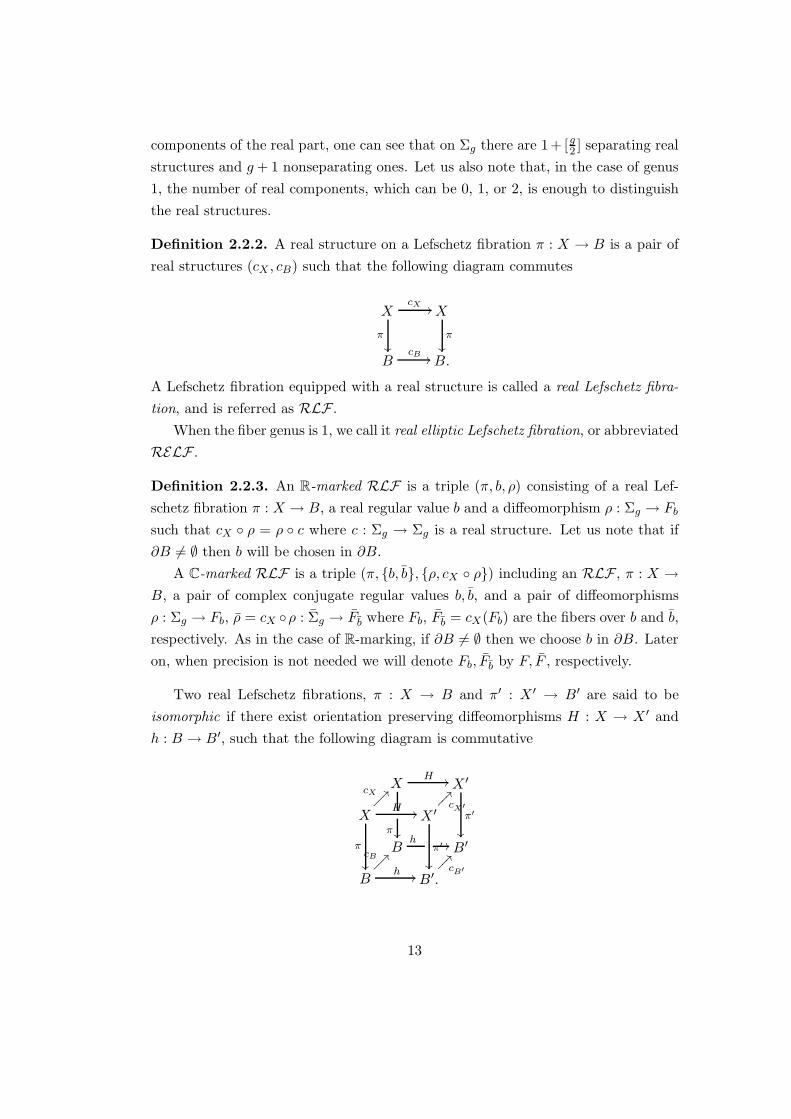
Definition 2.2.2. A real structure on a Lefschetz fibration π : X → B is a pair of
real structures (cX , cB) such that the following diagram commutes
XcX
//
π
X
π
BcB
// B.
A Lefschetz fibration equipped with a real structure is called a real Lefschetz fibra-
tion, and is referred as RLF .
When the fiber genus is 1, we call it real elliptic Lefschetz fibration, or abbreviated
RELF .
Definition 2.2.3. An R-marked RLF is a triple (π, b, ρ) consisting of a real Lef-
schetz fibration π : X → B, a real regular value b and a diffeomorphism ρ : Σg → Fb
such that cX ρ = ρ c where c : Σg → Σg is a real structure. Let us note that if
∂B 6= ∅ then b will be chosen in ∂B.
A C-marked RLF is a triple (π, b, b, ρ, cX ρ) including an RLF , π : X →B, a pair of complex conjugate regular values b, b, and a pair of diffeomorphisms
ρ : Σg → Fb, ρ = cX ρ : Σg → Fb where Fb, Fb = cX(Fb) are the fibers over b and b,
respectively. As in the case of R-marking, if ∂B 6= ∅ then we choose b in ∂B. Later
on, when precision is not needed we will denote Fb, Fb by F, F , respectively.
Two real Lefschetz fibrations, π : X → B and π′ : X ′ → B′ are said to be
isomorphic if there exist orientation preserving diffeomorphisms H : X → X ′ and
h : B → B′, such that the following diagram is commutative
XH
//
π
X ′
π′
X
cX ??
H//
π
X ′cX′
??
π′
Bh
// B′
Bh
//
cB ??
B′.cB′
??
13

Two R-marked RLFs, are called isomorphic if they are isomorphic as RLFs,h(b) = b′, and the following diagram is commutative
FH
//
cX
F ′
cX′
Σgρ′
::tttttρ
ddJJJJJ
c
FH
// F ′
Σg.ρ′
::ttttρ
ddJJJJJ
Two C-marked RLFs are called isomorphic if they are isomorphic as RLFs and
the following diagram is well defined and commutative
FH
//
cX
F ′
cX′
Σgρ′
::tttttρ
ddJJJJJ
id
FH
// F ′
Σg.ρ′
::ttttρ
ddJJJJJ
Definition 2.2.4. A real Lefschetz fibration π : X → B is called directed if the real
part of (B, cB) is oriented.
For example, if cB is separating then we consider an orientation on the real part
inherited from one of the halves B \ Fix(cB).
Two directed RLFs are isomorphic if they are isomorphic as RLFs with the
additional condition that the diffeomorphism h : B → B preserves the chosen ori-
entation on the real part.
Example 2.2.5. The construction given in Example 2.1.5 can be made equivariantly
to obtain an RLF . Namely, we pick out two generic real cubics C1, C2 in (CP 2, conj)
given by real degree three polynomials Q1, Q2 and consider, following Example 2.1.5,
the associated elliptic Lefschetz fibration CP 2#9CP 2 → CP 1. The set of 9 blown
up points and the fibration are clearly conj-invariant. In this way we obtain a real
E(1). Note that unlike in the complex case the real fibration does depend on the
choice of real cubics C1, C2 already since any even number of the 9 blown up points
can happen to be imaginary.
14
The fiber sum of two directed R-marked RLFs is defined as the fiber sum of
two marked LFs. Notice that by definition the gluing diffeomorphism is equivariant
once D2 is chosen equivariant. Evidently, the ultimate RLF is directed.
For RLFs without marking, one can start from choosing equivariantly diffeo-
morphic regular real fibers and then follow the construction with markings.
Remark 2.2.6. The construction of Example 2.2.5 can be applied to pencils of
curves of arbitrary degree d. In this way, we obtain RLFs over CP 1 ∼= S2 with
regular fibers diffeomorphic to a genus g = (d−1)(d−2)2 surface.
Definition 2.2.7. Let π : X → B be an LF . We define the conjugate LF as the
fibration π : X → B which coincides with π as a map and differs from the initial
LF only by changing the orientation of the base and the fibers.
To introduce a conjugate of a marked LF , we preselect an orientation reversing
diffeomorphism j : Σg → Σg and define the conjugate marked LF as (π, b, ρ j).
Remark 2.2.8. It is obvious that two conjugate Lefschetz fibrations have the same
set of critical points and critical values. Indeed, let ψ : U → C2 and φ : V → C be
the local charts of an LF such that φ π ψ−1 is (z1, z2) → z12 + z2
2. Then local
charts of the conjugate LF can be chosen as conj ψ : U → C2 and conj φ : V → C
with (z1, z2) → z21 + z2
2 .
Definition 2.2.9. An LF is called weakly real if it is equivalent to its conjugate,
or in other words if there exist an orientation reversing diffeomorphism, h, of B and
an orientation preserving diffeomorphism, H, of X such that the following diagram
commutes
XH
//
π
X
π
Bh
// B.
In particular, every RLF is weakly real. At this point, one can naturally doubt
if the converse is true or not. In case of g = 1, a partial answer will be given in
Section 3.7.
15

CHAPTER 3
factorization of the monodromy of
real lefschetz fibrations
3.1 Fundamental factorization theorem for real
Lefschetz fibrations
We will discuss below decomposability of the monodromy of real Lefschetz fibrations
over a 2-disc into a product of two involutions, presenting the real structures of the
two real fibers. This is a well-known fundamental fact, which we generalize to weakly
real Lefschetz fibrations in Theorem 3.1.2. The restriction of a Lefschetz fibration to
the boundary of the 2-disc is a usual fibration over a circle, and it will be convenient
to extend the terminology from the previous chapter to such fibrations.
More precisely, let π : Y → S1 be a fibration whose fiber is a compact connected
oriented smooth 2-manifold F . Shortly, such π will be called an F -fibration. In
particular, when the genus of F is equal to 1, we call π an elliptic F -fibration
Definition 3.1.1. An F -fibration π : Y → S1 is called weakly real if there is an
orientation preserving diffeomorphism H : Y → Y which sends fibers into fibers
reversing their orientations. If H2 = id, then H will be called a real structure on the
F -fibration Y → S1. An F -fibration equipped with a real structure will be called
real.
16

Note that H induces an orientation reversing diffeomorphism hS1 : S1 → S1
such that the following diagram commutes
YH
//
π
Y
π
S1h
S1// S1.
It is not difficult to see that the set of orientation reversing involutions form a
single conjugacy class in the diffeomorphism group of S1 (the crucial observation is
that any such involution has precisely two fixed points). So, any real F -fibration is
equivariantly isomorphic to an F -fibration whose involution hS1 is standard. Let it
be the complex conjugation cS1 : S1 → S1, z 7→ z, z ∈ S1 ⊂ C.
In the case of a weakly real F -fibration, hS1 may be not an involution, however,
it also has precisely two fixed points and can be changed into an involution by an
isotopy. It is not difficult to see that this isotopy can be lifted to an isotopy of H.
Thus, by modification of H we can always make hS1 an involution. So, it is not
restrictive for us to suppose always that hS1 = cS1 both for real and weakly real
F -fibrations.
The restrictions of H to the invariant fibers F± = π−1(±1) will be denoted
h± : F± → F±. In the case of real F -fibrations, we will prefer to use notation cY for
the involution H, and c± for the involutions h±.
It is well known that any F -fibration π : Y → S1 is isomorphic to the projection
Mf → S1 of a mapping torus Mf = F × I(f(x),0)∼(x,1) of some diffeomorphism
f : F → F . More precisely, if we fix a particular fiber F = Fb = π1(b), b ∈ S1, then
an isomorphism φ : Mf → Y can be chosen so that F × 0 and F × 1 are identified
with the fiber Fb, so that x× 0 7→ x and x× 1 7→ f(x).
An F -fibration π determines a diffeomorphism f up to isotopy and thus provides
a well-defined element in the mapping class group [f ] ∈ Map(F ) called the mon-
odromy of π (relative to the fiber F = Fb). A map f representing the class [f ] will
be also often called monodromy, or more precisely, a monodromy map.
In some cases, we fix a marking ρ : Σg → Fb. Then the diffeomorphism ρ−1fρ :
Σg → Σg (the pull-back of f) as well as its isotopy class [ρ−1 f ρ] ∈ Map(Σg) will
be called the monodromy of π relative to the marking ρ.
In what follows, we choose the point b in the upper semi-circle, S1+. The restric-
tion Y+ = π−1(S1+) → S1
+ of π admits a trivialization φ+ : Y+ → F × S1+ which is
identical on the fiber F = Fb. This allows us to consider the pull-back of c± via φ,
17

namely, the two involutions x 7→ φ+(c±(φ−1+ (x×±1))) on the same fiber F . We will
preserve notation c± for these involutions.
Theorem 3.1.2. Let π : Y → S1 be a weakly real F -fibration with a distinguished
fiber F = Fb, b ∈ S1+.
Then the two product diffeomorphisms of the fiber F , (h+)−1h−, and h+(h−)−1
are isotopic and describe the monodromy of π relative to the fiber F . In particular,
if π is a real F -fibration, then the monodromy can be factorized as f = c+ c−.
Proof. Consider a trivialization Y− → F×S1− of the restriction Y− = π−1(S1
−) →S1− of π over the lower semi-circle, S1
−, which is the composition of φ+ H : Y− →S1
+ × F , with the map F × S1+ → F × S1
−, (x, z) 7→ (x, cS1(z)).
b
x
x
x xx
x
x
xx
x
x
x
...
...
.
(1)
f
xxxxxxxxxxxxxxxxxxxxxxxxx
b
b
x
x
x xx
x
x
xx
x
x
x
...
...
c c
(2)
r r.. +-
+-
+
-
S1
S1
Fig. 3.1.
If S1 is split into several arcs and a fibration over S1 is glued from trivial fibra-
tions over these arc, then the monodromy is clearly the product of the gluing maps
of the fibers over the common points of the arcs, ordered in the counter-clockwise
direction beginning from a marked point b ∈ S1. In our case, the arcs are S1+,
S1−, their common points follow in the order −1, +1, and the corresponding gluing
maps, are h−1− and h+. This gives monodromy h+ (h−)−1. If we consider another
trivialization Y− → F × S1− replacing in its definition H by H−1, then the gluing
maps will be h− and h−1+ , and the monodromy is factorized as (h+)−1 h−. 2
Remark 3.1.3. It follows from Theorem 3.1.2 that the diffeomorphisms h−1 f has well as h f h−1, where h stands either for h+, or for h−, are all isotopic to
the inverse f−1 of the monodromy f of a weakly real F -fibration π (note that f−1
is the monodromy map of the conjugate F -fibration). In particular, if π is a real
F -fibration, then f−1 = c+ f c+ = c− f c−.
18

Corollary 3.1.4. Consider a weakly real F -fibration π : Y → S1, fix a trivialization
of π+ : Y+ → S1+, and consider the associated diffeomorphisms h± : F → F . Let
h stands for any of the four maps h±, h−1± . Then there exists a diffeomorphism
f : F → F representing the monodromy class [f ] ∈ Map(F ) of π, such that f−1 =
h f h−1.
In particular, if F -fibration π is real, then one can choose a monodromy map f
such that f−1 = c f c.
Definition 3.1.5. A diffeomorphism f : F → F as well as its isotopy class [f ] ∈Map(F ) will be called real (weakly real) if it is a monodromy of a real (weakly real,
respectively) F -fibration.
Proposition 3.1.6. An F -fibration is real (weakly real) if and only if its monodromy
f is real (weakly real).
Proof. We give the proof for real F -fibrations; the proof for weakly real ones is
analogous. Necessity of the condition in the Proposition is trivial. For proving the
converse, let π : Y → S1 be an F -fibration with the monodromy class [f ] ∈ Map(F ),
and f its representative such that f−1 = cf c, where c is some real structure on F .
Presenting Y as F ×I(f(x),0)∼(x,1), we obtain a well-defined involution cY : Y → Y
induced from the involution (x, t) 7→ (c(x), 1− t) in F × I. It preserves the fibration
structure and acts as c and f c on the real fibers F × 12 and F × 0 = F × 1 respec-
tively. 2
3.2 Homology monodromy factorization of elliptic F -
fibrations
We will characterize all real elliptic F -fibrations by answering the question: which
elements in Map(F ) are real in the case of torus, F = T ?
It is well known that Map(T ) = SL(2,Z), due to the fact that every diffeomor-
phism f : T → T is isotopic to a linear diffeomorphism. The latter diffeomorphisms
by definition are induced on T = R2/Z2 by a linear map R2 → R2 defined by a
matrix A ∈ SL(2,Z). Note that we can naturally identify T = H1(T,R)/H1(T,Z),
and interpret matrix A as the induced automorphism f∗ in H1(T,Z). The latter au-
tomorphism is called the homology monodromy. Since isotopic diffeomorphisms have
the same homology monodromy in H1(T,Z), we obtain well defined homomorphisms
19

Map(T ) → Aut+(H1(T,Z)) → SL(2,Z) which are in fact isomorphisms (here Aut+
stand for the orientation preserving automorphisms).
Let a denote the simple closed curve on T represented by the equivalence class
of the horizontal interval I × 0 ⊂ R2, and b is similarly represented by the vertical
interval 0 × I. We have a b = 1 hence, the homology classes represented by
these curves are integral generators of H1(T,Z). The mapping class group of T is
generated by the Dehn twists ta and tb, which can be characterized by their homology
monodromy homomorphism matrices ta∗ =(
1 0
1 1
)
, and tb∗ =(
1 −1
0 1
)
.
Therefore, for elliptic Lefschetz fibrations, the question of characterization of
real monodromy classes [f ] ∈ Map(T ) can be interpreted as the question on the
decomposability of their homology monodromy f∗ ∈ SL(2,Z) into a product of
two linear real structures. The latter structures by definition are linear orientation
reversing maps of order 2 defined by integral (2×2)-matrices. Such decomposability
is equivalent to the property that f∗ is conjugate to its inverse by a linear real
structure. Hence a necessary condition for a matrix A to be real is that both A and
A−1 lies in the same conjugacy classes in the group GL(2,Z).
Recall that there are three types of real structures on T distinguished by the
number of their real components: 0, 1, or 2. We will say that a real structure on T
is even if it has 0 or 2 components, and odd if it has 1 component. Note that the
automorphisms of H1(T,Z) induced by even real structures are diagonalizable over
Z, namely, their matrices are conjugate to(
1 0
0 −1
)
in GL(2,Z). So, we cannot
determine if the number of components 0 or 2 knowing only the matrix representing
the homology action of the real structure. The homology action of an odd real
structure is presented by a matrix conjugate to(
0 1
1 0
)
.
3.3 The modular action on the hyperbolic half-plane
Let C2 be considered as the vector space of 2 × 1 matrices over C. Then a matrix
A =(
a b
c d
)
in GL(2,Z) acts on C2 from the left as matrix multiplication.
(a b
c d
)(z1
z2
)
=
(az1 bz2
cz1 dz2
)
This action can be extended to CP 1 = C2 \ (0, 0)(z1 ,z2)∼(λz1,λz2) since
(a b
c d
)(λz1
λz2
)
=
(aλz1 λbz2
cλz1 λdz2
)
= λ
(az1 bz2
cz1 dz2
)
.
20

Let us identify CP 1 ∼= (z1, z2) ∈ C2, z2 6= 0 ∪ ∞ ∼= C ∪ ∞ and rewrite
the action of GL(2,Z). We obtain a linear fractional transformation z → az+bcz+d
where z = z1z2
. In particular, if A ∈ SL(2,Z), then the transformation preserves the
orientation of C and takes R∪∞ to itself preserving its orientation. Hence, it gives
rise to a diffeomorphism of the upper half plane H which can be seen as a model
for the hyperbolic plane where the geodesics are the semi-circles centered at a real
point or vertical half-lines which can also be considered as arcs of infinite radius. By
identifying the upper half plane with lower half plane by complex conjugation, one
extends the action of SL(2,Z) to an action of GL(2,Z). The standard fundamental
domain of the action is the set z| |Re(z)| ≤ 12 , |z| ≥ 1 which is shown in the Figure
below.
0-1 1-1/2 1/2
xxxxxxxxxxxxxxxxxxxxxxxxxxxxxxxxxxxxxxxxxxxxxxxxxxxxxxxxxxxxxxxxxxxxxxxxxxxxxxxxxxxxxxxxxxxxxxxxxxxxxxxxxxxxxxxxxxxxxxxxxxxxxxxxxxxxxxxxxxxxxxxxxxxxxxxxxxxxxxxxxxxxxxxxxxxxxxxxxxxxxxxxxxxxxxxxxxxxxxxxxxxxxxxxxxxxxxxxxxxxxxxxxxxxxxxxxxxxxxxxxxxxxxxxxxxxxxxxxxxxxxxxxxxxxxxxxxxxxxxxxxxxxxxxxxxxxxxxxxxxxxxxxxxxxxxxxxxxxxxxxxxxxxxxxxxxxxxxxxxxxxxxxxxxxxxxxxxxxxxxxxxxxxxxxxxxxxxxxxxxxxxxxxxxxxxxxxxxxxxxxxxxxxxxxxxxxxxxxxxxxxxxxxxxxxxxxxxxxxxxxxxxxxxxxxxxxxxxxxxxxxxxxxxxxxxxxxxxxxxxxxxxxxxxxxxxxxxxxxxxxxxxxxxxxxxxxxxxxxxxxxxxxxxxxxxxxxxxxxxxxxxxxxxxxxxxxxxxxxxxxxxxxxxxxxxxxxxxxxxxxxxxxxxxxxxxxxxxxxxxxxxxxxxxxxxxxxxxxxxxxxxxxxxxxxxxxxxxxxxxxxxxxxxxxxxxxxxxxxxxxxxxxxxxxxxxxxxxxxxxxxxxxxxxxxxxxxxxxxxxxxxxxxxxxxxxxxxxxxxxxxxxxxxxxxxxxxxxxxxxxxxxxxxxxxxxxxxxxxxxxxxxxxxxxxxxxxxxxxxxxxxxxxxxxxxxxxxxxxxxxxxxxxxxxxxxxxxxxxxxxxxxxxxxxxxxxxxxxxxxxxxxxxxxxxxxxxxxxxxxxxxxxxxxxxxxxxxxxxxxxxxxxxxxxxxxxxxxxxxxxxxxxxxxxxxxxxxxxxxxxxxxxxxxxxxxxxxxxxxxxxxxxxxxxxxxxxxxxxxxxxxxxxxxxxxxxxxxxxxxxxxxxxxxxxxxxxxxxxxxxxxxxxxxxxxxxxxxxxxxxxxxxxxxxxxxxxxxxxxxxxxxxxxxxxxxxxxxxxxxxxxxxxxxxxxxxxxxxxxxxxxxxxxxxxxxxxxxxxxxxxxxxxxxxxxxxxxxxxxxxxxxxxxxxxxxxxxxxxxxxxxxxxxxxxxxxxxxxxxxxxxxxxxxxxxxxxxxxxxxxxxxxxxxxxxxxxxxxxxxxxxxxxxxxxxxxxxxxxxxxxxxxxxxxxxxxxxxxxxxxxxxxxxxxxxxxxxxxxxxxxxxxxxxxxxxxxxxxxxxxxxxxxxxxxxxxxxxxxxxxxxxxxxxxxxxxxxxxxxxxxxxxxxxxxxxxxxxxxxxxxxxxxxxxxxxxxxxxxxxxxxxxxxxxxxxxxxxxxxxxxxxxxxxxxxxxxxxxxxxxxxxxxxxxxxxxxxxxxxxxxxxxxxxxxxxxxxxxxxxxxxxxxxxxxxxxxxxxxxxxxxxxxxxxxxxxxxxxxxxxxxxxxxxxxxxxxxxxxxxxxxxxxxxxxxxxxxxxxxxxxxxxxxxxxxxxxxxxxxxxxxxxxxxxxxxxxxxxxxxxxxxxxxxxxxxxxxxxxxxxxxxxxxxxxxxxxxxxxxxxxxxxxxxxxxxxxxxxxxxxxxxxxxxxxxxxxxxxxxxxxxxxxxxxxxxxxxxxxxxxxxxxxxxxxxxxxxxxxxxxxxxxxxxxxxxxxxxxxxxxxxxxxxxxxxxxxxxxxxxxxxxxxxxxxxxxxxxxxxxxxxxxxxxxxxxxxxxxxxxxxxxxxxxxxxxxxxxxxxxxxxxxxxxxxxxxxxxxxxxxxxxxxxxxxxxxxxxxxxxxxxxxxxxxxxxxxxxxxxxxxxxxxxxxxxxxxxxxxxxxxxxxxxxxxxxxxxxxxxxxxxxxxxxxxxxxxxxxxxxxxxxxxxxxxxxxxxxxxxxxxxxxxxxxxxxxxxxxxxxxxxxxxxxxxxxxxxxxxxxxxxxxxxxxxxxxxxxxxxxxxxxxxxxxxxxxxxxxxxxxxxxxxxxxxxxxxxxxxxxxxxxxxxxxxxxxxxxxxxxxxxxxxxxxxxxxxxxxxxxxxxxxxxxxxxxxxxxxxxxxxxxxxxxxxxxxxxxxxxxxxxxxxxxxxxxxxxxxxxxxxxxxxxxxxxxxxxxxxxxxxxxxxxxxxxxxxxxxxxxxxxxxxxxxxxxxxxxxxxxxxxxxxxxxxxxxxxxxxxxxxxxxxxxxxxxxxxxxxxxxxxxxxxxxxxxxxxxxxxxxxxxxxxxxxxxxxxxxxxxxxxxxxxxxxxxxxxxxxxxxxxxxxxxxxxxxxxxxxxxxxxxxxxxxxxxxxxxxxxxxxxxxxxxxxxxxxxxxxxxxxxxxxxxxxxxxxxxxxxxxxxxxxxxxxxxxxxxxxxxxxxxxxxxxxxxxxxxxxxxxxxxxxxxxxxxxxxxxxxxxxxxxxxxxxxxxxxxxxxxxxxxxxxxxxxxxxxxxxxxxxxxxxxxxxxxxxxxxxxxxxxxxxxxxxxxxxxxxxxxxxxxxxxxxxxxxxxxxxxxxxxxxxxxxxxxxxxxxxxxxxxxxxxxxxxxxxxxxxxxxxxxxxxxxxxxxxxxxxxxxxxxxxxxxxxxxxxxxxxxxxxxxxxxxxxxxxxxxxxxxxxxxxxxxxxxxxxxxxxxxxxxxxxxxxxxxxxxxxxxxxxxxxxxxxxxxxxxxxxxxxxxxxxxxxxxxxxxxxxxxxxxxxxxxxxxxxxxxxxxxxxxxxxxxxxxxxxxxxxxxxxxxxxxxxxxxxxxxxxxxxxxxxxxxxxxxxxxxxxxxxxxxxxxxxxxxxxxxxxxxxxxxxxxxxxxxxxxxxxxxxxxxxxxxxxxxxxxxxxxxxxxxxxxxxxxxxxxxxxxxxxxxxxxxxxxxxxxxxxxxxxxxxxxxxxxxxxxxxxxxxxxxxxxxxxxxxxxxxxxxxxxxxxxxxxxxxxxxxxxxxxxxxxxxxxxxxxxxxxxxxxxxxxxxxxxxxxxxxxxxxxxxxxxxxxxxxxxxxxxxxxxxxxxx
Fig. 3.2. The upper half plane model of hyperbolic space, and the standard fundamentaldomain of SL(2,Z).
3.4 The Farey Tessellation
Let us identify the upper half plane model with the Poincare disk model D. We will
consider the disk D together with its boundary R ∪∞ and define a tessellation on
D as follows:
Set ∞ as 10 and consider the two fractions 0
1 and 10 , spot them on D as the
south and the north poles respectively and connect them with a line which will be
the vertical diameter. Consider their mediant 0+11+0 = 1
1 and connect each of them
with a geodesic to the mediant. Apply the same to the fractions 01 ,
11 and 1
1 ,10.
Iterating this process one obtains a tessellation of the right semi-disk. By taking the
symmetry one extends the tessellation to D. (See Figure 3.3).
In the literature this tessellation is called the Farey tessellation. Let us denote
the disk together with the Farey tessellation by DF . Note that Farey tessellation is
21

0/1
1/0
1/1
0/1
1/0
1/1
2/1
1/2
3/1
3/2
2/3
1/3 0/1
1/0
1/1
2/1
1/2
3/1
3/2
2/3
1/3
-2/1
-1/1
-3/1
-3/2
-1/2
-2/3
-1/3
Fig. 3.3. Tessellation of D.
a tessellation of D by ideal triangles ( i.e. triangles with vertices on the boundary
DF ). In fact, the set of vertices of the triangles is exactly Q ∪ ∞. Moreover, two
fractions m1
n1, m2
n2are connected by a line iff m1n2 −m2n1 = ±1. Hence the action of
GL(2,Z) on D induces an action on DF which is transitive on the geodesics of DF.
Only ±I acts as the identity hence the modular group PGL(2,Z) = GL(2,Z)/ ± I
is the symmetry group of DF where the subgroup PSL(2,Z) = SL(2,Z)/ ± I gives
the orientation preserving symmetries. In what follows we denote by Γ the triangle
with vertices 0, 1,∞. Note that Γ splits in 3 copies of a fundamental region.
3.5 Elliptic and parabolic matrices
The fixed points of the modular action of a matrix A ∈ PSL(2,Z), A 6= I, in DF
are solutions of z = az+bcz+d . This gives a quadratic equation cz2 + (d − a)z − b = 0
with the discriminant (d − a)2 + 4bc = (d − a)2 + 4(ad − 1) = (a + d)2 − 4, and
we have 3 cases. If the trace |tr(A)| < 2 then the discriminant is negative and the
modular action is a rotation around an imaginary point (an interior point of DF ).
Such matrices are called elliptic. If |tr(A)| = 2, then the discriminant vanishes, and
A acts as a translation with one fixed rational point, d−a2 (on the boundary of DF ).
Such matrices are called parabolic. The hyperbolic matrices have |tr(A)| > 2 and
define a translation of DF with two fixed quadratically irrational real points (on the
boundary of DF ).
Elliptic Matrices: As mentioned above an elliptic matrix, A ∈ PSL(2,Z) act
on DF as rotation around a point in the interior of DF . The center of the rotation
belongs to one of the triangles of the tessellation. Without loss of generality let us
assume that the fixed point belongs to the triangle Γ. If the fixed point belongs to
an edge of Γ, then A rotates Γ by an angle π. The other possibility is rotation by
22

angle ±2π3 around the center of Γ. Note that the pair of rotations by angles ±2π
3
are conjugate to each other via an orientation reversing matrix from PGL(2,Z).
Since PGL(2,Z) acts transitively on the triangles of the tessellation rotation by
π around the center of an edge of Γ and rotation by 2π3 around the center of Γ defines
the conjugacy classes in PGL(2,Z) of elliptic matrices of PSL(2,Z).
0/1
1/0
1/1
2/1
1/2
3/1
3/2
2/3
1/3
-2/1
-1/1
-3/1
-3/2
-1/2
-2/3
-1/3
.π.
0/1
1/0
1/1
2/1
1/2
3/1
3/2
2/3
1/3
-2/1
-1/1
-3/1
-3/2
-1/2
-2/3
-1/3
.π/3
Fig. 3.4. Modular actions of elliptic matrices, Eπ,E 2π3
.
With respect to the triangle Γ, we can consider following matrices representing
these two conjugacy classes. Eπ =(
0 1
−1 0
)
, E 2π3
=(
0 1
−1 1
)
.
Each matrix A in PSL(2,Z) defines two matrices ±A in SL(2,Z). It is not
hard to see that the matrices ±Eπ are conjugate to each other via reflection with
respect to the edge containing the fixed point while ±E 2π3
are not, simply by the
fact that they have different traces. Hence, there are three conjugacy classes in
GL(2,Z), Eπ,±E 2π3
, of matrices in SL(2,Z) where E 2π3
gives the clockwise rotation
while −E 2π3
is conjugate to the clockwise rotation of DF with respect to the center
of the triangle Γ.
Parabolic Matrices: The fixed point of the action of a parabolic matrix in
PSL(2,Z) is rational, thus it is a common vertex of an infinite set of triangles of
DF . Since PGL(2,Z) acts transitively on the rational points, it is not restrictive to
assume that the fixed point of the translation is 0.
Hence, a parabolic element can shift the triangle Γ by arbitrary number n trian-
gles to the right or to the left(Figure 3.5) fixing 0. The left shift is conjugated to the
right shift by the reflection with respect to the vertical line. Hence the equivalence
classes in PGL(2,Z) are determined by the number n of shifts. Such a shift can be
represented by the matrix Pn =(
1 0
n 1
)
, n ∈ N.
23

0/1
1/0
1/1
2/1
1/2
3/1
3/2
2/3
1/3
-2/1
-1/1
-3/1
-3/2
-1/2
-2/3
-1/3 .
Fig. 3.5. Modular actions of parabolic matrices Pn.
The matrix Pn ∈ PSL(2,Z) corresponds to matrices ±Pn ∈ SL(2,Z). Note that
±Pn can not be in the same conjugacy class since they have different traces. Thus
the conjugacy classes in GL(2,Z) of parabolic matrices in SL(2,Z) are determined
by the integer ±n. A representative of conjugacy classes can be chosen as ±(
1 0
n 1
)
,
n ∈ N.
3.6 Hyperbolic matrices
A hyperbolic matrix A ∈ PSL(2,Z) acts on DF as translation fixing two irrational
points. The geodesic (a semicircle), lA, connecting these fixed points, oriented in
the direction of translation, remains invariant under the translation, so A preserves
also the set of the triangles of DF which are cut by lA.
0/1
1/0
1/1
2/1
1/2
3/1
3/2
2/3
1/3
-2/1
-1/1
-3/1
-3/2
-1/2
-2/3
-1/3
.
..
invariantgeodesic
Fig. 3.6. Modular action of a hyperbolic matrix.
With respect to the orientation of lA, such triangles are situated in two different
ways: a set of triangles with a common vertex lying on the left of lA followed by a
set of triangles with common vertex lying on the right of lA, see Figure 3.7.
24

0/1
1/0
1/1
2/1
1/2
3/1
3/2
2/3
1/3
-2/1
-1/1
-3/1
-3/2
-1/2
-2/3
-1/3
.l a
a
a1
2
3
a4
.........
......
......
...
a
a a1 3 n
2
a1
n
a
aa n
Fig. 3.7. Periodic pattern of the truncated triangles of the Farey tessellation.
Let us label right and left triangles by R and L, respectively. Then we encode
the arrangement of left and right triangles with respect to lA as an infinite word,
. . . LL . . . LRR . . . RLL . . . L . . ., of 2 letters. This word is called the cutting word
of lA. Let us fix a point p at the intersection of lA with an edge separating two
types of triangles. Relative to this point, we obtain a sequence, (a1, a2, a3, . . .)p,
from the cutting word where a2i−1 stands for the number of consecutive triangles
of one type while a2i, i = 1, 2, . . . is the number of consecutive triangles of the
other type. For example, if the cutting word with respect to p reduced to the word
LL . . . L︸ ︷︷ ︸
a1
RR . . . R︸ ︷︷ ︸
a2
LL . . . L︸ ︷︷ ︸
a3
. . . = La1Ra2La3 . . ., then we obtain (a1, a2, . . .)p. This
sequence is called the cutting sequence relative to the point p.
Left and right triangles form a periodic pattern and the action of A is a shift by
the period, so the cutting sequence has a period of even length. Note that choice
of the point p is not canonical, hence we can encode the period only as a cycle,
[a1a2 . . . a2n−1a2n]A, which we call the cutting period-cycle associated to the matrix
A.
Because of the fact that PGL(2,Z) is the full symmetry group of DF , the cut-
ting period-cycle of a hyperbolic matrix A ∈ PSL(2,Z) gives the complete in-
variant of the conjugacy class in PGL(2,Z) of A. In other words, two matrices
A,B ∈ PSL(2,Z) are in the same conjugacy class in PGL(2,Z) if and only if
[a1a2 . . . a2n]A = [aσ(1)aσ(2) . . . aσ(2n)]B for a cyclic permutation σ. Hence we will
denote the conjugacy classes in PGL(2,Z) of hyperbolic matrices of PSL(2,Z) by
the cycle [a1a2 . . . a2n] (defined up to cyclic ordering).
25

It can be seen geometrically that with respect to the triangle Γ a matrix repre-
senting a translation corresponding to the cutting period-cycle [a1, a2, . . . , an] can
be chosen as the following product of parabolic matrices.
(1 a1
0 1
) (1 0
a2 1
)
· · ·(
1 a2n−1
0 1
)(1 0
a2n 1
)
.
For the sake of simplicity, let us denote U =(
1 1
0 1
)
and V =(
1 0
1 1
)
. Then
the above product is written as Ua1V a2 . . . V a2n . Note that U is conjugate to V in
PGL(2,Z) but not in PSL(2,Z).
Let us note that in certain cases, namely if lA intersects the vertical line of DF ,
(since the action of PGL(2,Z) is transitive on the geodesics of DF , up to conjugation
this property is always satisfied), the cutting sequence of lA with respect to the
point of intersection of lA with the vertical line is related to the continued fraction
expansion of the fixed point, ξ, which is the “end point” of lA with respect to the
orientation. The corresponding theorem is due to C. Series [S1, S2].
Theorem 3.6.1 ([S1, S2]). Let x > 1, and let l be any geodesic ray joining some
point p on the vertical line of DF to x, oriented from p to x. Suppose that cutting
word of l with respect to p is La1Ra2La3 . . .. Then x = a1 + 1a2+ 1
a3+···
.
Note that if 0 < x < 1 then the sequence starts with R and x = 1a1+ 1
a2+ 1a3+···
.
If x < 0 everything applies with x replaced by −x and with R and L interchanged.
A matrix A ∈ PSL(2,Z) corresponds to ±A ∈ SL(2,Z). Since ±A have different
traces the cutting period-cycle [a1a2 . . . a2n]A, together with the sign determine the
conjugacy of ±A in GL(2,Z). A representative of the conjugacy classes of ±A can
be chosen as ±Ua1V a2 . . . V a2n .
3.7 Real factorization of elliptic and parabolic matrices
Let us first recall that the modular action of linear real structures(
1 0
0 −1
)
,(
0 1
1 0
)
on the hyperbolic plane D is z 7→ −z and z 7→ 1z
respectively. Geometrically, these
are reflections with respect to the vertical and, respectively, the horizontal lines, see
Figure 3.8. In particular, the first reflection takes our basic triangle Γ with vertices
0, 1,∞ to the triangle with vertices 0,−1,∞, and the second one takes Γ to
itself.
26

0/1
1/0
1/1
2/1
1/2
3/1
3/2
2/3
1/3
-2/1
-1/1
-3/1
-3/2
-1/2
-2/3
-1/3
Fig. 3.8. Modular actions of linear real structures.
Theorem 3.7.1. Every elliptic and parabolic matrices in SL(2,Z) is a product of
two linear real structures.
Proof. The explicit real decomposition for each conjugacy class of elliptic ma-
trices is given below.
E 2π3
=
(0 1
−1 1
)
=
(1 0
1 −1
) (0 1
1 0
)
−E 2π3
∼=(
−1 1
−1 0
)
=
(1 −1
0 −1
) (0 1
1 0
)
Eπ =
(0 1
−1 0
)
=
(1 0
0 −1
) (0 1
1 0
)
.
Figure 3.9 illustrates geometrically the above decompositions in terms of the
corresponding modular action of the matrices.
0/1
1/0
1/1
2/1
1/2
3/1
3/2
2/3
1/3
-2/1
-1/1
-3/1
-3/2
-1/2
-2/3
-1/3
.
0/1
1/0
1/1
2/1
1/2
3/1
3/2
2/3
1/3
-2/1
-1/1
-3/1
-3/2
-1/2
-2/3
-1/3
.
0/1
1/0
1/1
2/1
1/2
3/1
3/2
2/3
1/3
-2/1
-1/1
-3/1
-3/2
-1/2
-2/3
-1/3
.
Fig. 3.9. Decompositions of modular actions of elliptic matrices.
27

A real decomposition for each conjugacy class of parabolic matrices can be given
as follows.
Pn =
(1 0
n 1
)
=
(1 0
n −1
)(1 0
0 −1
)
−Pn =
(−1 0
−n −1
)
=
(1 0
n −1
)(−1 0
0 1
)
.
2
Example 3.7.2. Figure 3.10 shows the real decomposition of the modular action
of matrices(
1 0
n 1
)
for n = 1, 2.
0/1
1/0
1/1
2/1
1/2
3/1
3/2
2/3
1/3
-2/1
-1/1
-3/1
-3/2
-1/2
-2/3
-1/3.
0/1
1/0
1/1
2/1
1/2
3/1
3/2
2/3
1/3
-2/1
-1/1
-3/1
-3/2
-1/2
-2/3
-1/3.
Fig. 3.10. Decompositions of modular actions of parabolic matrices P1, P2.
3.8 Criterion of factorizability for hyperbolic matrices
Lemma 3.8.1. If the cutting period-cycle of a hyperbolic matrix A is [a1a2 . . . a2n]A,
then the cutting period-cycle of A−1 is [a2na2n−1 . . . a1]A−1 .
Proof. Note that lA = lA−1 with opposite orientation. So, the cutting word of
A−1 can be obtained from the cutting word of A by taking the mirror image of the
word and interchanging L with R. Interchanging L and R does not effect the cutting
period-cycle, hence the cutting period-cycle of A−1 is the reverse [a2na2n−1 . . . a1]A−1
of the cutting period-cycle [a1a2 . . . a2n] of A. 2
Definition 3.8.2. A finite sequence (a1a2 . . . ak) is called palindromic if it is equal
to the reversed sequence (akak−1 . . . a1). We call k the length of the sequence.
28

Definition 3.8.3. A cutting period-cycle is called bipalindromic if there is a cyclic
permutation of it such that the permuted period can be subdivided into two palin-
dromic sequences.
In particular, if the cutting period-cycle is subdivided into two palindromic se-
quences of odd length (even length) we call it odd-bipalindromic (respectively, even-
palindromic).
For example, if the period [1213] is odd-bipalindromic, while the period [1122] is
even-bipalindromic.
If A−1 = Q−1AQ for some Q ∈ PGL(2,Z) then by Lemma 3.8.1 we get that
[aσ(1), aσ(2), . . . , aσ(2n)] = [a2n, a2n−1, . . . , a1] for some cyclic permutation σ. This
implies that the cutting period-cycle [a1a2 . . . a2n] is bipalindromic.
Note that when the cutting period-cycle is odd-bipalindromic then the symmetry
of palindromic pieces lifts to a symmetry of left/ right triangles corresponding to
cutting period-cycle. This is not true for even-bipalindromic periods. For example,
for [1213] we have 121 ∼ LR2L = LRRL and 3 ∼ R3 = RRR while for [1122] we
have 11 ∼ LR and 22 ∼ L2R2 = LLRR.
Theorem 3.8.4. A hyperbolic matrix A is a product of two linear real structures if
and only if its cutting period-cycle [a1a2 . . . a2n]A is odd-bipalindromic.
Lemma 3.8.5. Let A ∈ PSL(2,Z) such that A−1 = Q−1AQ for some Q ∈ PGL(2,Z)
and let lA be the geodesic invariant under the action of A. Then Q(lA) = lA.
Proof. Clearly, if A(lA) = lA then A−1(lA) = lA. Hence,
A−1(lA) = Q−1AQ(lA) ⇔ Q(lA) = A(Q(lA)).
By the uniqueness of the invariant geodesic we get Q(lA) = lA. 2
Lemma 3.8.6. Let A,Q, lA as above. If the cutting period-cycle [a1a2 . . . a2n]A of
A is even-bipalindromic, then Q is orientation preserving.
Proof. By Lemma 3.8.5 we haveQ(lA) = lA, henceQ preserves triangles meeting
lA. The action of Q on DF is a linear fractional transformation, so it preserves
the angles. An analysis on the angles at meeting points of lA and the edges of
the triangles will forbid the existence of the orientation reversing map in the case
29

that the cutting period-cycle is even-bipalindromic. Let us assume that the cutting
period-cycle has the form
[a1a2 . . . akak . . . a2a1︸ ︷︷ ︸
P
a′1a′2 . . . a
′sa
′s . . . a2a
′1
︸ ︷︷ ︸
P ′
]
where s + k = n and P and P ′ are two palindromic pieces. Substituting the
pieces P,P ′ to the cutting sequence we obtain a sequence of P and P ′ of the form
PP ′PP ′ . . .. Clearly, the action of the matrix A on the sequence we obtain, corre-
sponds to a shift by two: it takes P to P , P ′ to P ′. Let us call edges which separate
the triangles corresponding to P from the triangles corresponding to P ′ as bound-
aries. There are two types of boundaries: if we go in the direction of translation
along lA we encounter boundaries where we pass from P to P ′ and boundaries where
we pass from P ′ to P . Let us denote such boundaries by ei and e′i respectively.
Each triangle of DF which is cut by lA splits into two pieces one of which is a
triangle. Let τi (τ ′i) be triangles having one edge ei (e′i, respectively) and obtained
as the union of triangle-pieces of triangles of DF with a common vertex of one side
of lA, see Figure 3.11. Let αi, (α′i) be the interior angles of τi (τ ′i , respectively)
between the edges ei (e′i, respectively) and lA. Let βi and β′i be the other interior
angles of τi and τ ′i corresponding to edges on lA.
Note that since A shift triangles by the period PP ′, A takes αi to αi+1 (similarly
α′i to α′
i+1). Hence all αi (similarly all α′i) are equal. Let α = αi for all i (and α′ = α′
i
for all i.)
0/1
1/0
1/1
2/1
1/2
3/1
3/2
2/3
1/3
-2/1
-1/1
-3/1
-3/2
-1/2
-2/3
-1/3
αxxxxxxxxxxxxxxxxxxxxxxxxxxxxxxxxxxxxxxxxxxxxxxxxxxxxxxxxxxxxxxxxxxxxxxxxxxxxxxxxxxxxxxxxxxxxxxxxxxxxxxxxxxxxxxxxxxxxxxxxxxxxxxxxxxxxxxxxxxxxxxxxxxxxxxxxxxxxxxxxxxxxxxxxxxxxxxxxxxxxxxxxxxxxxxxxxxxxxxxxxxxxxxxxxxxxxxxxxxxxxxxxxxxxxxxxxxxxxxxxxxxxxxxxxxxxxxxxxxxxxxxxxxxxxxxxxxxxxxxxxxxxxxxxxxxxxxxxxxxxxxxxxxxxxxxxxxxxxxxxxxxxxxxxxxxxxxxxxxxxxxxxxxxxxxxxxxxxxxxxxxxxxxxxxxxxxxxxxxxxxxxxxxxxxxxxxxxxxxxxxxxxxxxxxxxxxxxxxxxxxxxxxxxxxxxxxxxxxxxxxxxxxxxxxxxxxxxxxxxxxxxxxxxxxxxxxxxxxxxxxxxxxxxxxxxxxxxxxxxxxxxxxxxxxxxxxxxxxxxxxxxxxxxxxxxxxxxxxxxx
xxxxxxxxxxxxxxxxxxxxxxxxxxxxxxxxxxxxxxxxxxxxxxxxxxxxxxxxxxxxxxxxxxxxxxxxxxxxxxxxxxxxxxxxxxxxxxxxxxxxxxxxxxxxxxxxxxxxxxxxxxxxxxxxxxxxxxxxxxxxxxxxxxxxxxxxxxxxxxxxxxxxxxxxxxxxxxxxxxxxxxxxxxxxxxxxxxxxxxxxxxxxxxxxxxxxxxxxxxxxxxxx
αixxxxxxxxxxxxxxxxxxxxxxxxxxxxxxxxxxxxxxxxxxxxxxxxxxxxxxxxxxxxxxxxxxxxxxxxxxxxxxxxxxxxxxxxxxxxxxxxxxxxxxxxxxxxxxxxxxxxxxxxxxxxxxxxxxxxxxxxxxxxxxxxxxxxxxxxxxxxxxxxxxxxxxxxxxxxxxxxxxxxxxxxxxxxxxxxxxxxxxxxxxxxxxxxxxxxxxxxxxxxxxxxxxxxxxxxxxxxxxxxxxxxxxxxxxxxxxxxxxxxxxxxxxxxxxxxxxxxxxxxxxxxxxxxxxxxxxxxxxxxxxxxxxxxxxxxxxxxxxxxxxxxxxxxxxxxxxxxxxxxxxxxxxxxxxxxxxxxxxxxxxxxxxxxxxxxxxxxxxxxxxxxxxxxxxxxxxxxxxxxxxxxxxxxxxxxxxxxxxxxxxxxxxxxxxxxxxxxxxxxxxxxxxxxxxxxxxxxxxxxxxxxxxxxxxxxxxxxxxxxxxxxxxxxxxxxxxxxxxxxxxxxxxxxxxxxxxxxxxxxxxxxxxxxxxxxxxxxxxxxxxxxxxxxxxxxxxxxxxxxxxxxxxxxxxxxxxxxxxxxxxxxxxxxxxxxxxxxxxxxxxxxxxxxxxxxxxxxxxxxxxxxxxxxxxxxxxxxxxxxxxxxxxxxxxxxxxxxxxxxxxxxxxxxxxxxxxxxxxxxxxxxxxxxxxxxxxxxxxxxxxxxxxxxxxxxxxxxxxxxxxxxxxxxxxxxxxx
xxxxxxxxxxxx
xxxxxxxxxxxxxxx
iαi τiτ
i+1
' '
Fig. 3.11.
Moreover, there is an elliptic matrix in the conjugacy classes of Eπ which fixes
the point of intersection of lA with the middle edge of P or P ′(such edge exists since
30

the pieces have even length). Such matrix interchanges the edges ei to e′i. Hence
α = α′. (In the same way we obtain β = βi = β′i for all i.)
P
a aa
P'
e e' '
Fig. 3.12.
Let us assume that α < π2 . (If it is not so, we can replace α with β. Being two
interior angles of a triangle, α and β can not be both grater then π2 .)
0/1
1/0
1/1
2/1
1/2
3/1
3/2
2/3
1/3
-2/1
-1/1
-3/1
-3/2
-1/2
-2/3
-1/3
α
α
αββ
P
α αα
P'
vvv
vv v
111
222 ββ
Fig. 3.13.
Let us chose an orientation of DF by specifying (v1, v2) where v1 is a tangent
vector of lA and v2 is the tangent vector of ei or e′i such that the angle α between v1
and v2 is α < π2 , see Figure 3.13. The proof follows from the following observation.
The matrix Q takes (v1, v2) to itself since it preserves lA and the set of boundaries
of P and P ′ hence the angles between them. However, an orientation reversing map
can not preserve the angle both α < π2 between the vectors (v1, v2) and the vectors
at the same time.2
Proof of the Theorem 3.8.4 (⇒) The matrix A is a product of two liner
real structures, which implies that the cutting period-cycle is odd-bipalindromic by
Lemma 3.8.6.
31

(⇐) If the cutting period-cycle is odd-bipalindromic, then up to cyclic ordering,
the period cutting-cycle has two palindromic pieces of odd length. Let us assume
that the cutting period-cycle is of the form
[a1a2 . . . akak+1ak . . . a2a1a′1a
′2 . . . a
′sa
′s+1a
′s . . . a
′2a
′1]
where (2k+1)+(2s+1) = 2n. Then for some Q ∈ PGL(2,Z), we have B = Q−1AQ
such that B = Ua1V a2 . . . Ua2V a1Ua′1V a′
2 . . . Ua′2V a′
1 . Matrices Uai and V ai have the
following real decompositions,
Uai =
(1 −ai
0 −1
)(1 0
0 −1
)
andV ai =
(1 0
0 −1
)(1 0
−ai −1
)
.
Hence the product Ua1V a2 . . . Ua2V a1 can be rewritten in the form
(1 −a1
0 −1
)
· · ·(
1 0
−ak −1
)(1 −ak+1
0 −1
)(1 0
−ak −1
)
· · ·(
1 −a1
0 −1
)
.
This gives a linear real structure, since it is a conjugate of(
1 −ak+1
0 −1
)
. Sim-
ilarly, the product Ua′1V a′2 . . . Ua
′2V a′1 gives a linear real structure conjugate to
(1 −as+1
0 −1
)
. 2
Theorem 3.8.7. Every elliptic F -fibration is real if and only if it is weakly real.
Proof. Theorem follows from the following observations
(1) π : Y → S1 is real if and only if the monodromy f is real. i.e. f−1 = cf c,where c is a real structure. (Proposition 3.1.6).
(2) π : Y → S1 is weakly real if and only if the monodromy f is weakly real.
i.e. f−1 = h f h−1, where h is an orientation reversing diffeomorphism. (Propo-
sition 3.1.6).
(3) f−1 = c f c iff f−1 = h f h−1.
We only need to prove the observation (3).
Obviously f is real ⇒ f is weakly real.
For the converse note that, if f−1 = h f h, where h is orientation reversing,
then the cutting period-cycle [a1a2 . . . a2n−1a2n]f∗ of the corresponding homology
monodromy f∗ is odd-bipalindromic by Lemma 3.8.6. Then by Proposition 3.8.4,
we have f−1 = c f c, for a real structure c. 2
32

CHAPTER 4
real lefschetz fibrations around
singular fibers
It is well known that a singular fiber of a Lefschetz fibration is obtained from a nearby
regular fiber, F , by pinching a simple closed curve, a ⊂ F , the so-called vanishing
cycle. In a neighborhood of a singular fiber, a Lefschetz fibration is determined by
the monodromy, which is a positive Dehn twist, ta, along the vanishing cycle [K].
Recall that ta is a homeomorphism of F obtained by cutting F along a and gluing
back after one full twist in the positive direction.
In this chapter we classify and enumerate the real structures in a neighborhood
of a real singular fiber of a real Lefschetz fibration. Such a neighborhood can be
viewed as a Lefschetz fibration over a discD2 with a unique critical value q = 0 ∈ D2.
Without loss of generality, we may assume that the complex conjugation, conj in
D2 is the standard one, induced from C ⊃ D2. We call such fibrations elementary
Lefschetz fibrations (real or not). We start with an exposition of the techniques
giving the (well known) classification of Lefschetz fibrations in the non-real setting
and then generalize it for the real setting.
4.1 Elementary Lefschetz fibrations
Let (π : X → D2, b, ρ : Σg → Fb) be an elementary marked LF . By definition
there exist local charts (U, φU ), (V, φV ) around the critical point p ∈ π−1(0) and the
critical value 0 ∈ D2, respectively, such that U , V are closed discs and π|U : U → V
is isomorphic (via φU and φV ) to ξ : E → Dǫ, where E = (z1, z2) ∈ C2 : |z1| ≤
33

√ǫ,
∣∣z2
1 + z22
∣∣ ≤ ǫ2 and Dǫ = t ∈ C : |t| ≤ ǫ2, 0 < ǫ < 1 with ξ(z1, z2) = z2
1 + z22 .
Replacing the Lefschetz fibration by an isomorphic one over a smaller base, we can
assume that Dǫ = D2 and b ∈ ∂Dǫ and the critical value q = 0 ∈ Dǫ.
The projection (z1, z2) → z1 maps each fiber ξ−1(t) = (z1, z2) : z21 + z2
2 = tof ξ to the disc |z1| ≤ √
ǫ. This mapping represents the fiber ξ−1(t) as a two
sheeted covering ramified at z1 = ±√t. Therefore, topologically the regular fibers
ξ−1(t), t 6= 0, are cylinders and the fiber ξ−1(0) is a cone obtained from a nearby
fiber by pinching a simple closed curve, a, the vanishing cycle. Furthermore, such a
curve a realizes a non-trivial homology class in ξ−1(t) and, hence, it is unique up to
isotopy in ξ−1(t).
Recall that ∂E is naturally divided in two parts, ∂vE and ∂hE, see Defini-
tion 2.1.7. Let us fix a marking s : S1 × I → ξ−1(b), I = [0, 1]. Then, using the
double sheeted coverings of V ramified at z1 = ±√t, the vertical boundary ∂vE =
ξ−1(∂Dǫ) → ∂Dǫ can be identified with S1 × I × [0, 1](ta(x),0)∼(x,1) → [0, 1]0∼1
and the horizontal boundary ∂hE → Dǫ with S1 ×Dǫ → Dǫ.
The complement of U in π−1(V ) does not contain any critical point. Therefore,
X can be written as union of two LFs with boundary: one of them, U → V , is
isomorphic to E → Dǫ, and the other one is isomorphic to the trivial fiber bun-
dle R → Dǫ whose fibers are diffeomorphic to the complement of an open regular
neighborhood of the vanishing cycle a in Fb.
Let Ag be the set of isotopy classes of simple closed non-contractible (non-
oriented) curves on Σg, and let Vg be the set of isotopy classes of non-contractible
embeddings ν : S1 × I → Σg. We denote by Lg the set of isomorphism classes of
elementary marked genus-g Lefschetz fibrations and define Ω : Vg → Lg such that
Ω([ν]) = [Lν ] where [Lν ] stands for the isomorphism class of the Lefschetz fibration
Lν . The construction of Lν is as follows.
Let us choose a representative ν of [ν], and let Σνg denote the closure of Σg\ν(S1×
I). Consider the trivial fibration Rν = Σνg × Dǫ → Dǫ with horizontal boundary
∂Σνg × Dǫ → Dǫ. We take (ξ : E → Dǫ, b, s : S1 × I → ξ−1(b)) as above, switch
the marking to s ν−1 : ν(S1 × I) → ξ−1(b), and denote by Eν → Dǫ the marked
Lefschetz fibration (ξ : E → Dǫ, b, s ν−1 : ν(S1 × I) → ξ−1(b)). Then Lν → Dǫ
and its marking ρν : Σg → Fb is obtained by gluing Rν → Dǫ and Eν → Dǫ along
their trivial horizontal boundaries.
34

Lemma 4.1.1. Ω : Vg → Lg is a well defined map.
Proof. Let ν, ν ′ : S1 × I → Σg be two isotopic embeddings, and let ψt :
S1 × I → Σg, t ∈ [0, 1], be a continuous family of embeddings such that ψ0 = ν and
ψ1 = ν ′. Then, there exists an ambient isotopy Ψt : Σg → Σg such that Ψ0 = id and
ψt = Ψt ψ0. Clearly, Ψ1 induces diffeomorphisms Rν → Rν′ and Eν → Eν′ , which
respects the gluing and the fibrations, so that it gives an equivalence of Lν → Dǫ
and Lν′ → Dǫ as marked fibrations. Hence [Lν ] = [Lν′ ]. 2
We consider the map o : Vg → Ag such that o([ν]) = [ν(S1 ×12)] = [a]. Due to
the uniqueness of regular neighborhoods, the mapping o is a two sheeted covering:
the two elements of a fiber o−1([a]) corresponding to opposite orientations of a.
Since the automorphism (z1, z2) → (z1,−z2) of E → Dǫ is reversing the orientation
of the vanishing cycle (or, equivalently, since the Dehn twist does not depend on the
orientation on the vanishing cycle), the map Ω descends to a well defined map Ω
and the following diagram commutes
VgΩ
o// Ag
Ω~~||
||||
||
Lg.
Remark 4.1.2. The above diagram implies that the isomorphism class of resulting
fibration Lν → Dǫ does only depend on [a] = o([ν]). From now on we will denote
Lν by La.
Theorem 4.1.3. Ω : Ag → Lg is a bijection.
Proof. The surjectivity is already shown at the beginning of this section. Let
us show that Ω is injective. Consider [a], [a′] ∈ Ag such that Ωg([a]) = Ωg([a′]). We
will show that [a] = [a′]. Since Ω is well defined, for some representatives a, a′ of
[a], [a′] respectively, (La → Dǫ, b, ρν : Σg → Fb) is isomorphic to (La′ → Dǫ, b′, ρν′ :
Σg → F ′b′).
35

Then there exist orientation preserving diffeomorphisms H : La → La′ and
h : Dǫ → Dǫ such that we have the following commutative diagram
LaH
//
π
La′
π′
Dǫh
// Dǫ
where h(b) = b′ and H ρν = ρν′ .
The diffeomorphism H necessarily takes the critical point to the critical point
hence it takes the corresponding vanishing cycle a to a curve in a regular neighbor-
hood of a′. Since in a cylinder all non-contractible closed curves are isotopic, H(a)
is isotopic to a′. Moreover, since H ρ = ρ′, we have H(ρν(a)) = ρν′(a) and hence
ρν′(a) is isotopic to ρν′(a′).
Let ψt : F ′b′ → F ′
b′ , t ∈ [0, 1] such that ψ0 = id and ψ1(ρ′(a)) = ρ′(a′). Then
Ψt = ρ′−1 ψt ρ′ : Σg → Σg provides an isotopy from a to a′. 2
To deal with Lefschetz fibrations without marking we introduce the following
definition. Two simple closed curves, a and a′, on Σg are called conjugate if there
is an orientation preserving diffeomorphism of Σg which carries a to a′. Note that
isomorphic LFs give conjugate vanishing cycles by the following evident lemma.
Lemma 4.1.4. If there exists a diffeomorphism φ : Σg → Σg such that φ(a) is
isotopic to a then there exists a diffeomorphism ψ of Σg with ψ(a) = a′. 2
Proposition 4.1.5. There is a one-to-one correspondence between the classes of
elementary Lefschetz fibrations (non-marked) and the set of conjugacy classes of
non-contractible simple closed curves on Σg.
Proof. The proposition follows from Lemma 4.1.4 and Theorem 4.1.3. 2
Corollary 4.1.6. There are 1+[g2 ] isomorphism classes of elementary (non-marked)
genus-g Lefschetz fibrations.
Proof. Topologically, there are two types of simple closed curves on Σg: sepa-
rating and nonseparating. Up to diffeomorphism there exists only one nonseparating
curve.
The separating curves are determined by how they divide the genus in two pos-
itive integer summands (the summands are positive because we should exclude the
36

case when the curve bounds a disc in Σg, since pinching such a curve creates a sphere
with self intersection -1). Hence, totally we obtain 1 + [g2 ] many local models. 2
4.2 Elementary Real Lefschetz fibrations
Let (π : X → D2, b, ρ : Σg → Fb) be an R-marked elementary real Lefschetz
fibration. We classify such fibrations up to isomorphism then obtain a classification
of C-marked and non-marked RLFs.As in the non-real case, there exist equivariant local charts (U, φU ), (V, φV )
around the critical point p ∈ π−1(0) and the critical value 0 ∈ D2, respectively,
such that U and V are closed discs and π|U : (U, cU ) → (V, conj ) is equivariantly
isomorphic (via φU and φV ) to either of ξ± : (E±, conj ) → (Dǫ, conj ), where
E± = (z1, z2) ∈ C2 : |z1| ≤√ǫ,
∣∣z2
1 ± z22
∣∣ ≤ ǫ2
Dǫ = t ∈ C : |t| ≤ ǫ2, 0 < ǫ < 1
with ξ±(z1, z2) = z21 ± z2
2 ,
The above two real local models ξ± : E± → Dǫ can be seen as two real structures
on ξ : E → Dǫ. These two real structures are not equivalent. The difference can be
seen already at the level of the singular fibers: in the case of ξ+ the two branches
are imaginary and they are interchanged by the complex conjugation; in the case of
ξ− the two branches are both real (see Figure 4.1 where the two halves of the cone
correspond to the two branches so that the real structure becomes a corresponding
reflection).
To understand the action of the real structures on the regular real fibers of ξ±,
we can use the branched covering defined by the projection (z1, z2) → z1. Thus, we
obtain that:
• in the case of ξ+, there are two types of real regular fibers; the fibers Ft with
t < 0 have no real points, their vanishing cycles have invariant representatives
(that is c(at) = at set-theoretically), and in this case, c acts on the invariant
vanishing cycles as an antipodal involution; the fibers Ft with t > 0 has a circle
as their real part and this circle is an invariant, pointwise fixed, representative
of the vanishing cycle;
37

c
c
z + z z - z1
2 2222
21
real part
=0 =0
Fig. 4.1. Actions of real structures on the singular fibers of ξ±.
• in the case of ξ−, all the real regular fibers are of the same type and the
real part of such a fiber consists of two arcs each having its endpoints on the
two different boundary components of the fiber; the vanishing cycles have still
invariant representatives and c acts on them as a reflection.
(In Figure 4.2, all types of the real regular fibers and vanishing cycles of ξ± are
shown.)
z + z1222
Real Part
= -r
0 r-r
z + z1222=rz + z1
222=0
z + z1222(z , z )1 2
c ca a
z - z1222
Real Part
= -r
0 r-r
z - z1222 =rz - z1
222 =0
z - z1222(z , z )
1 2
c c
a a
Fig. 4.2. Nearby regular fibers of ξ± and vanishing cycles.
Using once more the ramified covering (z1, z2) → z1, we observe that the horizon-
tal part of the fibration ξ± is equivariantly trivial and, moreover, has a distinguished
equivariant trivialization. On the other hand, since the complement of U in π−1(V )
does not contain any critical point, X can be written as union of two RLFs with
boundary: one of them, U → V , is isomorphic to ξ± : E± → Dǫ, and the other one
is isomorphic to the trivial real fiber bundle R→ Dǫ whose fibers are equivariantly
38

diffeomorphic to the complement of an open regular neighborhood of the vanishing
cycle a in Fb. The two types of models, with ξ+ and with ξ−, can also be distin-
guished by the action of the complex conjugation on the boundary components of
the real fiber of R → Dǫ: in the case of ξ+ it switches the boundary components,
and in the case of ξ− they are preserved (and the complex conjugation acts as a
reflection on each of them).
Let Acg denote the set of equivariant isotopy classes of non-contractible curves
on the real surface (Σg, c) such that c(a) = a, and Vcg the set of equivariant isotopy
classes of non-contractible embeddings ν : S1 × I → Σg such that c ν = ν and LR,cg
the set of classes of directed R-marked elementary genus-g real Lefschetz fibrations.
Let [ν]c ∈ Vcg . We consider the map Ωc : Vcg → LR,cg such that Ωc([ν]c) =
[LRν ]c, where [LR
ν ]c denote the isomorphism class of directed R-marked real Lefschetz
fibration LRν . The construction of LR
ν is the equivariant version of the construction
of Lν . Let ν be a representative of [ν]c, we consider Σνg which is the closure of
Σg \ ν(S1 × I). Since c ν = ν, the surface Σνg inherits a real structure from
(Σg, c). On the boundary of Σνg the real structure acts in two ways, either it switches
two boundary components or acts as reflection on each boundary components. We
consider a trivial real fibration Rν = Σνg×Dǫ → Dǫ where cRν = (c, conj ) : Rν → Rν
is the real structure. Let Eν± → Dǫ denote the model ξ± : E → Dǫ whose marked
fiber is identified with ν(S1 × I). Depending on the real structure on the horizontal
boundary S1×Dǫ → Dǫ (where the real structure on S1×Dǫ is taken as (c∂Σνg, conj ))
of Rν → Dǫ, we choose either of Eν± → Dǫ and then glue Rν → Dǫ and the suitable
model Eν± → Dǫ along their horizontal trivial boundaries.
Lemma 4.2.1. Ωc : Vcg → LR,cg is well defined.
Proof. Let ν, ν ′ : S1 × I → Σg be two c-equivariant isotopic embeddings, and
let ψt : S1 × I → Σg, t ∈ [0, 1], be a continuous family of equivariant embeddings
such that ψ0 = ν and ψ1 = ν ′. Then, there exists an equivariant ambient isotopy
Ψt : Σg → Σg such that Ψ0 = id and ψt = Ψt ψ0 with Ψt c = c Ψt for all
t. Hence Ψ1 induces an equivariant diffeomorphisms Rν → Rν′ and Eν± → Eν′±,
which respects the fibrations, and the gluing thus it gives an equivalence of LRν → Dǫ
and LR
ν′ → Dǫ as R-marked fibrations. 2
Since c ν = ν, we have c(ν(S1 × 12)) = ν(S1 × 1
2)). Hence we can define
oc : Vcg → Acg such that o([ν]c) = [ν(S1 × 1
2)]c = [a]c. As in the case of LFs the
mapping oc is two-to-one. Since the monodromy does not depend on the orientation
39

of the vanishing cycle, there exists a well defined mapping, Ωc, such that the following
diagram commutes
VcgΩc
oc// Ac
g
Ωc
LR,cg .
Theorem 4.2.2. Ωc : Acg → LR,c
g is a bijection.
Proof. The proof is the equivariant version of the proof of 4.1.3. Let us denote
the image of Ωc by [LRa ]c. As it is discussed in the beginning of the section, any
elementary RLF can be divided equivariantly into two RLFs with boundary: an
equivariant neighborhood of the critical point (isomorphic to one of the models, ξ±),
and the complement of this neighborhood (isomorphic to a trivial real Lefschetz fi-
bration). Such a decomposition defines the equivariant isotopy class of the vanishing
cycle. This gives the surjectivity of Ωc.
To show that Ωc is injective let us consider [a]c, [a′]c ∈ Vcg such that Ωc([a]c) =
Ωc([a′]c). We will show that [a]c = [a′]c. Since Ωc is well defined we have [LRa ]c =
[LR
a′ ]c hence there exist equivariant orientation preserving diffeomorphismsH : LRa →
LR
a′ and h : Dǫ → Dǫ such that we have the following commutative diagrams
LRa
H//
π
LR
a′
π′
LRa
cLR
a ??H
//
π
LR
a′
cLR
a′
??
π′
Dǫh
// Dǫ
Dǫh
//
conj ??
Dǫconj
??
FH
//
cLR
a
F ′
cLR
a′
Σg
ρν′
::tttttρν
ddJJJJJ
c
FH
// F ′
Σg.ρν′
::ttttρν
ddJJJJJ
Clearly, H(ρν(a)) is equivariantly isotopic to ρν′(a′) where a and a′ are repre-
sentatives of [a]c and [a′]c respectively. Moreover, we have H ρν = ρν′ which gives
H(ρ(a)) = ρ′(a), so ρ′(a) is equivariant isotopic to ρ′(a′). Let ψt : F ′ → F ′,
t ∈ [0, 1] such that ψ0 = id and ψ1(ρ′(a)) = ρ′(a′), ψt c′ = c′ ψt. Then
Ψt = ρ′−1 ψt ρ′ : Σg → Σg is the required isotopy. 2
Theorem 4.2.2 shows that c-equivariant isotopy classes of vanishing cycles classify
the directed R-marked elementary RLFs. To obtain a classification for directed C-
marked RLFs we study the difference between two markings. We will be also
interested in the classification of non-marked RLFs.
40

m
m
b
F
FF
m
bm
Σgx
m
mx
cc
ρ
ρρb
Fig. 4.3.
A C-marking on a directed elementary RLF defines an R-marking up to iso-
topy. Let (m, m, ρm, cX ρm) be a C-marking on a directed RLF , π : X → D2.
The complement, ∂D2 \ m, m, has two pieces S± (upper/ lower semicircles) dis-
tinguished by the direction. By considering a trivialization of the fibration over
the piece of S+ connecting m to the real point, b, (the trivialization over the piece
connecting m to the real point obtain by the symmetry), we can pull the marking,
ρm : Σg → Fm, to Fb to obtain a marking, say ρb : Σg → Fb and a real structure
c = ρ−1b cX ρb : Σg → Σg. Any other trivialization results in an other marking
isotopic to ρb and a real structure isotopic to c : Σg → Σg.
Hence directed elementary C-marked RLFs defines a vanishing cycle defined up
to c-equivariant isotopy where the real structure c is considered up to isotopy.
Definition 4.2.3. A pair (c, a) of a real structure c : Σg → Σg and a non-
contractible simple closed curve a ∈ Σg, is called a real code of an elementary RLFif c(a) = a. Two real codes, (c0, a0), (c1, a1), will be called isotopic if there exist
an isotopy (ct, at), t ∈ [0, 1] such that ct(at) = at, ∀t. Moreover, two real codes,
(c0, a0) and (c1, a1), will be called conjugate if there is an orientation preserving
diffeomorphism φ : Σg → Σg such that φ c0 = c1 φ and that [φ(a0)]c1 = [a1]c1 .
We denote the isotopy class of the real code, (c, a), by [c, a] and the conjugacy class
by c, a.
Proposition 4.2.4. There is a one-to-one correspondence between the isomorphism
classes of directed C-marked elementary RLFs and the isotopy classes of real codes.
Proof. Let LC,[c]g denote the set of classes of directed C-marked elementary
genus-g real Lefschetz fibrations and A[c]g denote the isotopy classes, [c, a], of real
codes. We consider the map ω : LCg → A[c]
g . As it is discussed above, a directed
C-marked elementary RLF determines an isotopy class of a directed R-marked
41

elementary RLF . By Theorem 4.2.2 we obtain a vanishing cycle up to c-equivariant
isotopy. Since the real structure c is also determined up to isotopy we obtain the
real code [c, a]. Evidently, isomorphic directed C-marked elementary RLFs give
isotopic real codes. Hence ω is well-defined. Surjectivity of ω is also clear.
For the injectivity, we consider two isotopy classes [ci, ai], i = 1, 2 such that
[c1, a1] = [c2, a2]. Let (π1 : X1 → D2, m1, m1, ρm1, ρm1
) and (π2 : X2 →D2, m2, m2, ρm2
, ρm2) be two directed C-marked elementary RLFs, associated
to the classes [c1, a1] and [c2, a2], respectively. We need to show that π1 and π2 are
isomorphic as directed C-marked RLFs.Note that we can always choose a representative c for both [c1] and [c2] such that
[a1]c = [a2]c. Then by Theorem 4.2.2, π1 is isomorphic to π2 as R-marking RLFs.An isomorphism of R-marked RLFs may not preserve the C-markings. However, it
can be modified to preserve the C-markings:
b
m
m2
1S
S
+
+
1
Fig. 4.4.
Up to homotopy, one can identify X2 with a subset of X1. Letπ2:
X2→ D2 be
the corresponding fibration. Then, one can transformm2 to m1 preserving the real
marking and the trivializations over the corresponding paths, S+ andS+, see Fig-
ure 4.4 to obtain an isomorphism of C-marked RLFs, preserving the isomorphism
of R-marked RLFs. Since the difference X1\X2 has no singular fiber. 2
For fibrations without marking we allow to change [c, a] by an equivariant dif-
feomorphism. Hence we have the following proposition.
Proposition 4.2.5. There is a one-to-one correspondence between the set of con-
jugacy classes, c, a, of real codes and the set of classes of directed non-marked
elementary real Lefschetz fibrations. 2
42

4.3 Vanishing cycles of real Lefschetz fibrations
By definition any real code, (c, a), of directed elementary RLF satisfies c(a) = a.
Hence, the real structure acts on the vanishing cycle a. Such an action can be either
the identity, or an antipodal map, or a reflection. In the latter case, there are two
points fixed by c. They either belong to the same or different real components of c.
We call the curves on which c acts as an antipodal map totally imaginary and
those curves on which c acts as a reflection real-imaginary. (Recall that the curves
on which c acts as the identity are called real.)
In Figure 4.5 we show an invariant curve a together with the action of c. When
necessary, on figures, we will distinguish invariant curves by showing the action of
the real structure c.
Real curve Totally imaginary curve Real-imaginary curve
Fig. 4.5. Invariant curves together with the action of real structures.
Lemma 4.3.1. Let c be a real structure on a closed surface Σg, let a be an embedded
simple closed curve on Σg such that c(a) = a then c′ = ta c ( as well as c′′ = c ta)is a real structure on Σg.
Moreover, if a is real with respect to c then a is totally imaginary with respect to
c′, and vice versa. On the other hand, a is real-imaginary with respect to c if and
only if a is real-imaginary with respect to c′.
Proof. Clearly ta c is an orientation reversing diffeomorphism of Σg. Since c
is orientation reversing, the conjugation c ta c coincides with t−1c(a)
. Then we have
(ta c)2 = ta c ta c = ta t−1c(a) = ta t−1
a = id. This shows that ta c is a real
structure on Σg. (The proof of the case c ta is analogous.)
As for the second part, let us first recall the definition of the Dehn twist on
Σg along a. Let ν(a) be a regular neighborhood of a. We choose an orientation
preserving diffeomorphism φ : S1 × [0, 1] → ν(a) such that φ(S1 × 12) = a and
consider τ : S1 × [0, 1] → S1 × [0, 1] such that τ(θ, t) = (θ + 2πt, t). The Dehn twist
ta along a is the diffeomorphism obtained by taking φ τ φ−1 : ν(a) → ν(a) on
ν(a) and extending it to Σg by the identity. In particular, ta rotates a by an angle
43

of π. Hence, c|a is the identity if and only if (ta c)|a is the antipodal map and c|ais reflection if and only if (ta c)|a is reflection. See Figure 4.6. 2
ac ac a
c
RF RFa
RF
RF
Fig. 4.6. Actions of the real structure on nearby regular fibers of ξ±.
The next example shows a real surface together with some non-contractible c-
invariant curves.
Example 4.3.2. Let c′ be a reflection on a genus-5 surface whose real part is the
set of curves a1, a2, a3, a4 shown in Figure 4.7. We set c = ta1 c′ and consider
the real surface (Σ5, c). Figure 4.7 shows some examples of invariant curves on the
real surface (Σ5, c). Lemma 4.3.1 implies that c acts on a1 as the antipodal map,
hence the curve a1 is totally imaginary, while a2, a3, a4 are real. The curves, a5 and
a6 are real-imaginary. The real points of a5 belong to two different real curves, a2
and a3, whereas the real points of a6 belong to the real curve a4. Note that the
curves a1, a2, a3, a4, a5, a6 are nonseparating. While the curve a7 is an example of
separating real-imaginary curve.
a a a a
aa
1 2 3
5
4
6a7
Real curve Totally imaginary curve Real-imaginary curve
Fig. 4.7. c-invariant curves on (Σ5, c). We showed explicitly the action of c ona1, a2, a3, a4, a5, a6, a7.
44

4.4 Classification of elementary real Lefschetz fibrations
with nonseparating vanishing cycles
Let S∗g be the set of classes of real closed genus-g surfaces ( g ≥ 1) with two marked
points which are, as a set, invariant under the action of real structure and let Lcgbe the set of classes of directed non-marked elementary genus-g RLFs. We assume
that the vanishing cycle is nonseparating and define a map e : Lcg → S∗g−1 as follows.
Given a directed elementary RLF , we consider the associated real code (c, a). We
take a c-invariant regular closed neighborhood, ν(a), of a in (Σg, c). The complement
Σν(a)g = Σg \ ν(a) inherits the real structure from Σg and can be seen as a real
surface with two punctures. Let us consider the punctures as marked points on the
closed surface and define the image of e as the closed marked surface we obtain.
By construction the pair of marked points is invariant under the action of the real
structure. Clearly, equivalent real codes give equivalent real genus-(g − 1) surfaces,
hence e is well defined.
Lemma 4.4.1. The map e : Lcg → S∗g−1 is surjective.
Proof. Given (Σg−1, cg−1), a representative of a class in S∗g−1, by Proposi-
tion 4.2.5 it is enough to assign to it, a real code (c, a). Let s1, s2 be the marked
points on Σg−1, consider open neighborhoods ν(s1) , ν(s2) of s1 and s2, respectively
such that,
• if s1 and s2 are real then we have cg−1(ν(si)) = ν(si) for i = 1, 2,
• if one is the conjugate of the other then we set ν(s2) = cg−1(ν(s1)).
The complement, Σνg−1, of the neighborhoods ν(si), i = 1, 2, in Σg−1 is a real surface
with two boundary components. We consider S1 × [0, 1] and glue it to Σνg−1 along
the boundary components. The resulting surface has genus g.
The real structure of Σνg−1 can be extended to S1×[0, 1] to obtain a real structure
c on Σg such that a = S1 ×12 is a c-invariant curve. Thus, we obtain c : Σg → Σg
and a ⊂ Σg such that c(a) = a.
Clearly, any other representative (Σ′g−1, c
′g−1) give another code which is conju-
gate to (c, a). 2
45

Lemma 4.4.2.
|S∗g−1| =
9g−5
2 if g-1 even,9g−6
2 if g-1 odd.
Proof. Note that an invariant pair of marked points on a real surface can be
chosen:
• as a pair of complex conjugate points,
• as real points on a real component, if there is at least one real component,
• as real points on two different real components, if there are at least 2 real
components.
Up to equivariant diffeomorphisms such choices are unique. Thus, for each real
structure which has at least two real components we have 3 choices. When there is
only one real component, we get 2 choices and lastly if there are no real component,
we get only 1 choice for marked points. Recall that for each genus there is only one
real structure with no real component. There is one real structure with one real
component, if genus is odd and there are two such real structures if genus is even.
Since on Σg−1 there are g + 1 + [g−12 ] real structures, we obtain
|S∗g−1| = 3(g + 1 + [
g − 1
2]) − kwhere
k = 4 if g-1 even,
k = 3 if g-1 odd.
2
Proposition 4.4.3.
|Lcg| =
6 if g=1,
8g − 3 if g>1 odd,
8g − 4 if g>1 even.
Proof. Since e is surjective we will count the inverse images of (Σg−1, cg−1)
∈ S∗g−1. By Proposition 4.2.5, it is enough to count the real codes of elementary
RLFs.Case 1: Let (Σg−1, cg−1) be a real surface with a pair of conjugate marked
points, say s1, s2. As we discussed above we obtain the genus-g surface by gluing a
cylinder to the surface Σνg−1. Note that if marked points are conjugate pairs the real
structure switches the boundary components Σνg−1. Hence on the cylinder S1× [0, 1]
we consider a real structure which exchanges the boundaries. There are two such
46

real structures. One has a real component which is the central curve the other has
no real component. Hence, we have two inverse images for each real surface Σg−1.
...
*
*
... ...Real curve Totally imaginarycurve
Fig. 4.8. Gluing neighborhood of the vanishing cycle to a real genus-(g − 1) surface withtwo complex conjugated marked points.
Since the points, s1, s2 are not real, there is no condition on the number of real
components, so there are exactly 2(g + 1 + [g−12 ]) directed elementary RLFs.
Case 2: Let us assume that two marked points are chosen on a real component
of the real genus-(g − 1) surface. In this case, the real structure on the boundary
components of Σνg−1 is reflection hence each component has two real points. Recall
that there is a unique real structure up to diffeomorphism on the cylinder where
the action on the boundary is reflection. However, if we extend the real structure of
Σνg−1 to the cylinder we have two choices to connect the real points. These choices
result in different real structures since their number of real components are not the
same.
Excluding the case when the real structure has no real component we obtain
2(g + [g−12 ]) many local models.
Case 3: Finally, let us assume that the marked points are real points belonging
to different real components. This case can occur only if g−1 > 0. As in the case 2,
boundary components of Σνg−1 have two real points. Unlike the previous case, the
way we connect the real points does not effect the number of real components, see
Figure 4.10. However, it may change the type of the real structure.
Namely, if cg−1 is separating then we may obtain either separating or nonsep-
arating real structure. When cg−1 is nonseparating the resulting real structure is
nonseparating regardless of how we connect the real points.
47

...
... ...
Real curve* *
Real curves
Real curve
* *
Two real components One real component
Fig. 4.9. Gluing neighborhood of the vanishing cycle to a real genus-(g − 1) surface withtwo real marked points belonging to the same real component.
There are exactly g nonseparating real structures on a genus-(g − 1) surface.
Among nonseparating real structures there is one without real component and one
with a unique real component. The number of separating real structures on a genus-
(g− 1) surface whose real part has at least two real components is 1 + [g−12 ] if g− 1
is odd and [g−12 ] if g − 1 is even.
Hence, totally we have
g − 2 + 2(1 + [g−12 ]) real structures if g − 1 is odd and
g − 2 + 2[g−12 ] real structures if g − 1 is even.
Therefore,
• If g = 1, we have only cases 1 and 2, hence there are 4 + 2 = 6 directed
non-marked elementary RLFs with nonseparating vanishing cycle,
• if g > 1, is even then we have 2(g+1+[g−12 ])+2(g+[g−1
2 ])+2(1+[g−12 ])+g−2 =
8g − 4 directed non-marked elementary RLFs with nonseparating vanishing
cycle,
48

... Real curves
* *
... Real curve ... Real curve
* *
One real component One real component
Fig. 4.10. Gluing neighborhood of the vanishing cycle to a real genus-(g − 1) surface withtwo real marked points belonging to different real components.
• if g > 1, odd we have 2(g + 1 + [g−12 ]) + 2(g + [g−1
2 ]) + 2[g−12 ] + g− 2 = 8g − 3
directed non-marked elementary RLFs with nonseparating vanishing cycle.
2
4.5 Classification of elementary real Lefschetz fibrations
with separating vanishing cycles
In this section, we consider the real code (c, a) of an elementary RLF such that
a ⊂ Σg is a separating curve. Recall that we restrict ourselves to the study of
relatively minimal LFs. That is no fiber contains an exceptional sphere. Such
phenomenon corresponds to the case when the vanishing cycle bounds a disc. Hence,
we will assume that the vanishing cycle a does not bound a disc.
As before c acts on a. This action can be the identity, the antipodal map or
reflection. However, since a is separating if c acts on a as a reflection then two real
points of a necessarily belong to the same real component.
49
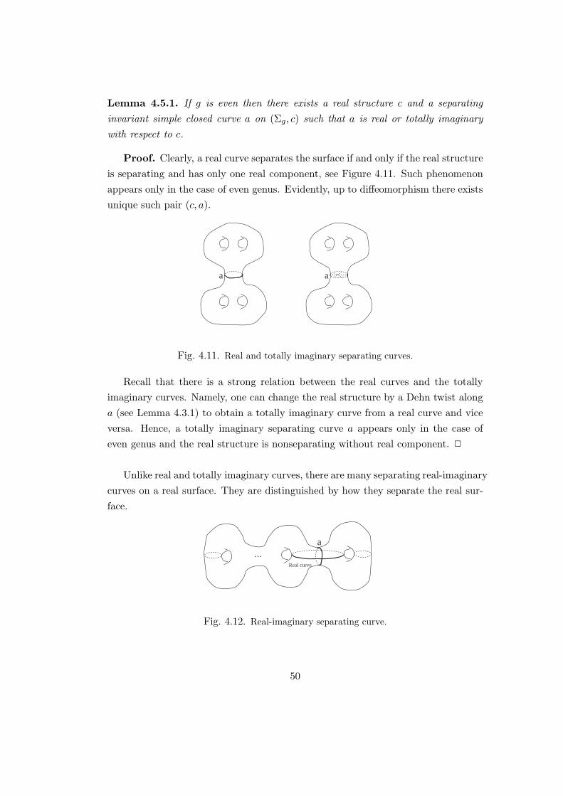
Lemma 4.5.1. If g is even then there exists a real structure c and a separating
invariant simple closed curve a on (Σg, c) such that a is real or totally imaginary
with respect to c.
Proof. Clearly, a real curve separates the surface if and only if the real structure
is separating and has only one real component, see Figure 4.11. Such phenomenon
appears only in the case of even genus. Evidently, up to diffeomorphism there exists
unique such pair (c, a).
a a
Fig. 4.11. Real and totally imaginary separating curves.
Recall that there is a strong relation between the real curves and the totally
imaginary curves. Namely, one can change the real structure by a Dehn twist along
a (see Lemma 4.3.1) to obtain a totally imaginary curve from a real curve and vice
versa. Hence, a totally imaginary separating curve a appears only in the case of
even genus and the real structure is nonseparating without real component. 2
Unlike real and totally imaginary curves, there are many separating real-imaginary
curves on a real surface. They are distinguished by how they separate the real sur-
face.
...Real curve
a
Fig. 4.12. Real-imaginary separating curve.
50

Note that if there is a real-imaginary curve then the real structure has necessarily
at least one real component. Let us fix a real surface (Σg, c) of genus g ≥ 1 such
that c has at least one real component. Then to calculate the possible separating
curves we will make use of the quotient Σg/c. For a nonseparating real structure c
on a genus-g surface with k > 0 real components, the quotient Σg/c is a disc with
k − 1 holes and l = g − k + 1 cross caps see Figure 4.13.
...
a
...
... ...
Fig. 4.13.
If the real structure is separating, the quotient Σg/c is an orientable genus g+1−k2
surface with k boundary components, see Figure 4.14. By abuse of notation we will
denote g+1−k2 also by l.
...
...
a
...
...
Fig. 4.14.
Hence in either case we have the following calculations.
Lemma 4.5.2. If both k−1 and l are even numbers then we have [k(l+1)2 ] separating
curves. Otherwise there are [k(l+1)2 ] − 1 separating curves.
Proof. This is a counting problem. A separating curve on Σg gives an arc on
Σg/c with endpoints lying on one of the boundary components. We count how many
different ways we can divide Σg/c by a such an arc.
When both k− 1 and l are even the arc can divide the Σg/c into two symmetric
pieces, Figure 4.15. Excluding such case we have (k−1+1)(l+1)−12 choices. Hence,
totally we obtain (k−1+1)(l+1)−12 +1. Finally, by subtracting the case when the curve
bounds a disc we obtain (k−1+1)(l+1)−12 + 1 − 1 = [ (k)(l+1)
2 ] such arc.
51

a a
Fig. 4.15. Examples of k = 3, l = 2.
When k− 1 or l is odd, we repeat the same idea. Note that in this case, such an
arc can not divide Σg/c symmetrically, hence we get (k−1+1)(l+1)2 −1 = [ (k)(l+1)
2 ]−1. 2
Proposition 4.5.3. The number of conjugacy classes of real codes c, a where a is
a separating curve is given as follows. By Proposition 4.2.5 this gives the number of
classes of directed R-marked elementary RLFs whose vanishing cycle is separating.
g even
g > 0
1 +∑
k∈1,3,...,g+1
l even
[k(l+1)2 ] +
∑
k∈1,3,...,g+1
l odd
([k(l+1)2 ] − 1) if c is separating,
1 +∑
k∈1,2,...,g
l even
[k(l+1)2 ] +
∑
k∈1,2,...,g
l odd
([k(l+1)2 ] − 1) if c is nonseparating,
g odd
∑
k∈2,4,...,g+1
([k(l+1)2 ] − 1) if c is separating,
∑
k∈1,2,...,g
([k(l+1)2 ] − 1) if c is nonseparating.
Proof. The proposition follows from Lemma 4.5.1 and Lemma 4.5.2.
Note that if c is nonseparating then k − 1 + l = g. Thus,
if g > 0 is even: (k − 1, l) = (even, even) or (k − 1, l) = (odd, odd)
if g is odd: (k − 1, l) = (even, odd) or (k − 1, l) = (odd, even).
52

If c is separating then k − 1 + 2l = g. Thus,
if g is even: (k − 1, l) = (even, even) or (k − 1, l) = (even, odd)
if g is odd: (k − 1, l) = (odd, even) or (k − 1, l) = (odd, odd).
2
53

CHAPTER 5
invariants of real lefschetz
fibrations with only real critical
values
The classification of elementary RLFs can be used to obtain certain invariants
for RLFs over a disc with only real critical values. For this reason we introduce
boundary fiber sum of real directed Lefschetz fibrations over D2. We will study
separately the cases of the fiber genus g > 1 and g = 1, since they are of different
nature with respect to the boundary fiber sum. On the other hand, if we assume
that fibration admits a real section then the case of g = 1 can be treated similar to
the case g > 1.
5.1 Boundary fiber sum of genus-g real Lefschetz fibra-
tions
Let π : X → D2 be a directed real Lefschetz fibration. Following the notation of
previous sections, we denote by S± the upper/ lower semicircles of ∂D2. We consider
also left/ right semicircles, denoted by S±, and the quarter-circles S±± = S± ∩ S±.
(Here directions right/ left and up/ down are determined by the orientation of
the real part.) Let r± be the real points of S±, and c± the real structures on
F± = π−1(r±).
54

S
S
S+++
-
--S+
-
r r+-
Fig. 5.1.
Definition 5.1.1. Let (π′ : X ′ → D2, b′, b′, ρ′, ρ′) and (π : X → D2, b, b,ρ, ρ) be two directed C-marked real Lefschetz fibrations such that the real struc-
tures c′+ on F ′+ and c− on F− induce (via the markings) isotopic real structures on
Σg. Then we define the boundary fiber sum, X ′ΣgX → D2D2, of C-marked RLFsas follows.
r'+
F'F'
b'+
b'
b'
Σg ρ
F
b
b
r
Fb
-
-
ρ'
c' c+ -
Fig. 5.2.
We choose trivializations of π′−1(S++) and π−1(S−
+) such that the pull backs of c′+
and c− give the same real structure c on Σg. Then the trivialization of π′−1(S+) can
be obtained as a union Σg ×S++ ∪Σg ×S+
−(x,1+)∼(c(x),1−) and similarly π−1(S−) =
Σg × S−+ ∪ Σg × S−
−(x,−1+)∼(c(x),−1−). Then the boundary fiber sum X ′ΣgX →D2D2 is obtained by gluing π′−1(S+) to π−1(S−) via the identity map.
Remark 5.1.2. 1. In fact, the construction described above creates a manifold with
corners but there is a canonical way to smooth the corners, hence the boundary fiber
sum is the manifold obtained by smoothing the corners.
2. By definition, the boundary fiber sum is associative but not commutative.
3. The boundary fiber sum of C-marked RLFs is naturally C-marked.
4. Note that D2D2 = D2 so when the precision is not needed we use D2 instead
of D2D2.
55

Proposition 5.1.3. If g > 1, then the boundary fiber sum, X ′ΣgX → D2, of
directed C-marked genus-g real Lefschetz fibrations is well-defined up to isomorphism
of C-marked RLFs.
Proof. Note that the boundary fiber sum does not effect the fibrations out-
side a small neighborhood of the intervals where the gluing is made. Let us slice a
topological disc D, a neighborhood (which does not contain a critical value) of the
gluing interval on D2 = D2D2. Let c′+ and c− denote the real structures on the
real fibers over the real boundary points of D, see Figure 5.3. Since D contains no
real critical value, real structures c′+, c− induce isotopic real structures on Σg. Hence
each real fibration over a disc without a critical value defines a path in the space of
real structures on Σg. Therefore, the difference of two boundary fiber sums gives a
loop in this space. The proof follows from contractibility of such loops discussed in
the next section, see Proposition 5.2.4. 2
b
b
.
xxxxxxxxxxxxxxxxxxxxxxxxxxxxxxxxxxxxxxxxxxxxxxxxxxxxxxxxxxxxxxxxxxxxxxxxxxxxxxxxxxxxxxxxxxxxxxxxxxxxxxxxxxxxxxxxxxxxxxxxxxxxxxxxxxxxxxxxxxxxxxxxxxxxxxxxxxxxxxxxxxxxxxxxxxxxxxxxxxxxxxxxxxxxxxxxxxxxxxxxxxxxxxxxxxxxxxxxxxxxxxxxxxxxxxxxxxxxxxxxxxxxxxxxxxxxxxxxxxxxxxxxxxxxxxxxxxxxxxxxxxxxxxxxxxxxxxxxxxxxxxxxxxxxxxxxxxxxxxxxxxxxxxxxxxxxxxxxxxxxxxxxxxxxxxxxxxxxxxxxxxxxxxxxxxxxxxxxxxxxxxxxxxxxxxxxxxxxxxxxxxxxxxxxxxxxxxxxxxxxxxxxxxxxxxxxxxxxxxxxxxxxxxxxxxxxxxxxxxxxxxxxxxxxxxxxxxxxxxxxxxxxxxxxxxxxxxxxxxxxxxxxxxxxxxxxxxxxxxxxxxxxxxxxxxxxxxxxxxxxxxxxxxxxxxxxxxxxxxxxxxxxxxxxxxxxxxxxxxxxxxxxxxxxxxxxxxxxxxxxxxxxxxxxxxxxxxxxxxxxxxxxxxxxxxxxxxxxxxxxxxxxxxxxxxxxxxxxxxxxxxxxxxxxxxxxxxxxxxxxxxxxxxxxxxxxxxxxxxxxxxxxxxxxxxxxxxxxxxxxxxxxxxxxxxxxxxxxxxxxxxxxxxxxxxxxxxxxxxxxxxxxxxxxxxxxxxxxxxxxxxxxxxxxxxxxxxxxxxxxxxxxxxxxxxxxxxxxxxxxxxxxxxxxxxxxxxxxxxxxxxxxxxxxxxxxxxxxxxxxxxxxxxxxxxxxxxxxxxxxxxxxxxxxxxxxxxxxxxxxxxxxxxxxxxxxxxxxxxxxxxxxxxxxxxxxxxxxxxxxxxxxxxxxxxxxxxxxxxxx
+
xxxxxxxxxxxxxxxxxxxxxxxxxxxxxxxxxxxxxxxxxxxxxxxxxxxxxxxxxxxxxxxxxxxxxxxxxxxxxxxxxxxxxxxxxxxxxxxxxxxxxxxxxxxxxxxxxxxxxxxxxxxxxxxxxxxxxxxxxxxxxxxxxxxxxxxxxxxxxxxxxxxxxxxxxxxxxxxxxxxxxxxxxxxxxxxxxxxxxxxxxxxxxxxxxxxxxxxxxxxxxxxxxxxxxxxxxxxxxxxxxxxxxxxxxxxxxxxxxxxxxxxxxxxxxxxxxxxxxxxxxxxxxxxxxxxxxxxxxxxxxxxxxxxxxxxxxxxxxxxxxxxxxxxxxxxxxxxxxxxxxxxxxxxxxxxxxxxxxxxx
FF' -c' c+ -
r r- +
Fig. 5.3.
5.2 Equivariant diffeomorphisms and the space of real
structures
Let Cc(Σg) denote the space of real structures on Σg which are isotopic to a fixed
real structure c, and let Diff0 (Σg) denote the group of orientation preserving dif-
feomorphisms of Σg which are isotopic to the identity. We consider the subgroup
of Diff0 (Σg), denoted Diff c0 (Σg), consisting of those diffeomorphisms which com-
mute with c and the subgroup Diff0 (Σg, c) of Diff0 (Σg) consisting of diffeomor-
phisms which are c-equivariantly isotopic to the identity. Note that the group
Diff0 (Σg) acts transitively on Cc(Σg) by conjugation. The stabilizer of this action is
56

the group Diff c0 (Σg). Hence Cc(Σg) can be identified with the homogeneous space
Diff0 (Σg)/Diff c0 (Σg).
Lemma 5.2.1. If g > 1 then Diff c0 (Σg) is connected for all c : Σg → Σg. However,
for g = 1, the space Diff c0 (Σg) is connected if c is an odd real structure (i.e. it has
1 real component).
Proof. (We will use different techniques for g > 1 and g = 1.) Let us first
discuss the case of g > 1. To show that Diff c0 (Σg) is connected, we consider the
fiber bundle description of conformal structures on Σg, introduced in [EE]. Let
Conf Σgdenote the space of conformal structures on Σg equipped with C∞-topology.
The group Diff0 (Σg) acts on Conf Σgby composition from right. This action is
proper, continuous, and effective hence Conf Σg→ Conf Σg
/Diff0 (Σg) is a principle
Diff0 (Σg)-fiber bundle, (cf. [EE]). The quotient is the Teichmuller space of Σg,
denoted TeichΣg . Note that conformal structures can be seen as equivalence classes
of Riemannian metrics with respect to the relation that two Riemannian metrics are
equivalent if they differ by a positive function on Σg. Let RiemΣg denote the space
of Riemannian metrics on Σg then we have the following fibrations
u : Σg → R : u > 0 // RiemΣg
p2
Diff0 (Σg) // Conf Σg
p1
TeichΣg.
The real structure c acts on Diff0 (Σg) by conjugation. This action can be ex-
tended to Conf Σgand RiemΣg as follows. We fix a section s : TeichΣg → Conf Σg
of
the bundle p1 and we consider a family of diffeomorphisms φsζ : Diff0 (Σg) → p−11 (ζ)
parametrized by TeichΣg such that φsζ(id) = s(ζ). Let [µx] denote a conformal struc-
ture where µx is a Riemannian metric on Σg. Then we have φsζ(f(x)) = [µf(x)] for all
f ∈ Diff0 (Σg), in particular φsζ(id) = s(ζ) = [µx]. The action of real structure, then,
can be written as c.[µf(x)] = [µcfc(x)]. Clearly the definition does not depend on
the choice of the representative of the class [µf(x)] so the action extends to RiemΣg .
Let FixConf Σg(c) denote the set of fixed points of the action of c on Conf Σg
and
FixRiemΣg(c), the set of fixed points on RiemΣg . Note that s(ζ) is in FixConf Σg
(c),
∀ζ ∈ TeichΣg . In fact each [µf(x)] where f ∈ Diff c0 (Σ1) is in FixConf Σg
(c). Our aim
is the show that FixConf Σg(c) is connected.
57

Note that if FixConf Σg(c) is disconnected then the inverse image (which is
FixRiemΣg(c)) is also disconnected in RiemΣg . It is known that RiemΣg is con-
vex and hence FixRiemΣg(c) is convex. However this contradicts to disconnectivity,
therefore FixConf Σg(c) is connected. Then FixConf Σg
(c) ∩Diff0 (Σg) = Diff c0 (Σg) is
connected since FixConf Σg(c) is a union of sections.
For the case of g = 1, we consider the quotient Σ1/c which is a Mobius band
(MB) when c is an odd structure. It is known that the space of diffeomorphisms
of Mobius band has two components: the identity component Diff0 (Σ1/c), and the
component of diffeomorphisms isotopic to the reflection h shown in Figure 5.4. Note
that when the Mobius band is obtained by from I × I by identifying appropriate
points of I × 0 with the points of I × 1, the diffeomorphism h can be seen as the
diffeomorphism induced from the reflection of I × I with respect to the I × 12 . The
diffeomorphism h is not isotopic to the identity, since before identifying the ends it
reverses the orientation of I × I.
real part
Mobius Band Real Torus
h
Fig. 5.4.
The diffeomorphism h lifts to the central symmetry h : Σ1 → Σ1 of Σ1. Central
symmetry is not isotopic to the identity on Σ1 since it reverses the orientation of
the real curve. Hence, we have
f : Σ1/c→ Σ1/c : f : Σ1 → Σ1 is isotopic to id = f : Σ1/c→ Σ1/c : f ∼= id.
The former is identified by Diff c0 (Σ1) and the latter is connected, hence Diff c
0 (Σ1)
is connected. 2
58

Lemma 5.2.2. For any real structure c : Σg → Σg
π1(Diff0 (Σg)/Diff0 (Σg, c), [id]) =
0 if g > 1
Z if g = 1
Proof. (When it is not needed we will omit the base point from the notation.)
Note that the subgroup Diff0 (Σg, c) acts from the left on Diff0 by composition.
Diff0 (Σg, c) × Diff0 (Σg) → Diff0 (Σg)
(f, g) → f g
Such action is free so Diff0 (Σg) → Diff0 (Σg)/Diff0 (Σg, c) is a Diff0 (Σg, c)-fiber
bundle. We consider the following long exact homotopy sequence of this fibration
...→ π2(Diff0 (Σg)) → π2(Diff0 (Σg)/Diff0 (Σg, c)) → π1(Diff0 (Σg, c)) →π1(Diff0 (Σg)) → π1(Diff0 (Σg)/Diff0 (Σg, c)) → π0(Diff0 (Σg)) → ...
Case of g > 1: it is known that Diff0 (Σg) is contractible if g > 1, so we have
πk(Diff0 (Σg), id) = 0 for all k [EE]. Using the exact homotopy sequence we obtain
π1(Diff0 (Σg)/Diff0 (Σg, c), [id]) ∼= π0(Diff0 (Σg, c), id).
Note that the group Diff0 (Σg, c) is isomorphic to Diff0 (Σg/c). Moreover, since
for any real structure c the Euler characteristic of Σg/c is negative, Diff0 (Σg/c) is
contractible [ES]. Hence, π1(Diff0 (Σg)/Diff0 (Σg, c), [id]) = 0.
Case of g = 1: it is known that Σ1 is deformation retract of Diff0 (Σ1). Hence up
to homotopy we consider Diff0 (Σ1) as a group generated by two rotations, shown in
Figure 5.5.
• If c has 2 real components, we consider an identification of Σ1 by C/Z2 such
that the real structure c is induced from the standard complex conjugation on C.
Let : C/Z2 → Σ1 be such an identification.
59

l
l
1
2
Fig. 5.5. Rotations generating Diff0 (Σ1).
We consider the following family of diffeomorphisms for t ∈ [0, 1],
R′1(t) : C/Z2 → C/Z2
(x+ iy)Z2 → (x+ t+ iy)Z2
R′2(t) : C/Z2 → C/Z2
(x+ iy)Z2 → (x+ i(y + t))Z2 .
where (x+ iy)Z2 denotes the equivalence class of x+ iy in C/Z2.
Note that R′i(0) = R′
i(1) = id and each R′i(t), t ∈ [0, 1] is isotopic to identity.
Hence Ri(t) = R′i(t) −1, i = 1, 2 form a bases of Diff0 (Σ1).
To understand Diff0 (Σ1, c) ⊂ Diff0 (Σ1) we consider the quotient Σ1/c which is
topologically an annulus. It is known that πk(Diff0 (Σ1/c), id) = πk(Diff0 (S1), id)
[I]. Hence, using the fact Diff0 (Σg, c) = Diff0 (Σg/c) we get
πk(Diff0 (Σ1, c), id) =
0 if k > 1
Z if k = 1
C
Fig. 5.6.
60

Note that with respect to the identification , diffeomorphismsR1(t) ∈ Diff0 (Σ1, c),
∀t ∈ [0, 1], hence R1(t) gives a loop in π1(Diff0 (Σ1, c), id). Thus we choose R1(t) as
a generator of π1(Diff0 (Σ1, c), id) = Z. Then from the exact sequence
0 → π1(Diff0 (Σg, c))f ′→ π1(Diff0 (Σg))
g′→ π1(Diff0 (Σg)/Diff0 (Σg, c)) → 0
0 → Zf ′→ Z + Z
g′→ π1(Diff0 (Σg)/Diff0 (Σg, c)) → 0
1 → (1, 0)
we get Im(f ′) = ker(g′) = π1(Diff0 (Σ1)/Diff0 (Σ1, c), [id]) = Z.
• If c has no real component, we consider : R2/Z2 → Σ1 such that the real
structure c is induced from the real structure c′ where
c′ = −1 c : R2/Z2 → R/Z2
(x, y)Z2 → (x+ 12 ,−y)Z2 .
Then we consider the family of diffeomorphisms R′i(t) : R2/Z2 → R2/Z2, t ∈
[0, 1] such that
R′1(t) : R2/Z2 → R2/Z2 R′
2(t) : R2/Z2 → R2/Z2
(x, y)Z2 → (x+ t, y)Z2 (x, y)Z2 → (x, y + t)Z2 .
Hence Ri(t) = R′i(t) −1, i = 1, 2 form a bases of Diff0 (Σ1). As above to
understand Diff0 (Σ1, c) we consider the quotient Σ1/c is a Klein bottle (KB). It is
known that Diff0 (KB) ∼= S1, [EE]. Hence we consider Diff0 (Σ1/c) as a group gener-
ated by the rotation which lifts to a translation in the universal cover of Klein bottle.
Such translation in the lattice and corresponding rotation shown in Figure 5.7.
Shift
Fig. 5.7.
61

Since Diff0 (Σ1, c) ∼= Diff0 (Σ1/c) ∼= S1 we have π1(Diff0 (Σ1, c), id) = Z. With
respect to the identification and the real structure c, R1(t) gives a generator of
π1(Diff0 (Σ1, c), id) = Z. Then from the exact sequence
0 → π1(Diff0 (Σ1, c)) → π1(Diff0 (Σ1)) → π1(Diff0 (Σ1)/Diff0 (Σ1, c)) → 0
1 → (1, 0)
we get π1(Diff0 (Σ1)/Diff0 (Σ1, c), [id]) = Z.
• If c is an odd real structure, Σ1 has unique real component, denoted C. The
restriction of f ∈ Diff0 (Σ1, c) to C defines a diffeomorphism of C. This restriction
gives a fibration with fibers isomorphic to
Diff0 (Σ1, C) = f ∈ Diff0 (Σ1, c) : f |C = id.
Note that Diff0 (Σ1, C) ∼= Diff0 (Σ1 \ C, ∂) where Σ1 \ C denote the closure of Σ1 \C and Diff0 (Σ1 \ C, ∂) diffeomorphisms of Σ1 \ C which are the identity on the
boundary. Note that Σ1 \ C is an annulus. It is known that Diff0 (Σ1 \ C, ∂) is
contractible [I]. Hence from the exact sequence of the fibration
Diff0 (Σ1,C) // Diff0 (Σ1, c)
Diff0 (C)
we get πk(Diff0 (Σ1, c), id) ∼= πk(Diff0 (C), id), ∀k.Let us choose the identification : C/Λ → Σ1 where Λ is the lattice generated
by v1 = (12 ,
12 ) and v2 = (1
2 ,−12), see Figure 5.8. Then the real structure c can be
taken as the one induced from the complex conjugation on C.
We consider R′i(t) : C/Λ → C/Λ, t ∈ [0, 1] such that
R′1(t) : C/Z2 → C/Z2 R′
2(t) : C/Z2 → C/Z2
(x+ iy)Λ → (x+ t+ iy)Λ (x+ iy)Λ → (x+ i(y + t))Λ.
Clearly, Ri(t) = R′i(t) −1 gives a bases for Diff0 (Σ1), since R1(t) commutes
with the real structure gives a generator for π1(Diff0 (Σ1, c)) = Z.
62

v
v
2
1
1
2
-1
1
2
-1
Fig. 5.8.
Therefore, we have
0 → π1(Diff0 (Σg, c))f→ π1(Diff0 (Σg))
g→ π1(Diff0 (Σg)/Diff0 (Σg, c)) → 0
0 → Zf→ Z + Z
g→ π1(Diff0 (Σ1)/Diff0 (Σ1, c)) → 0
1 → (1, 0)
Since the sequence is exact
Im(f) = ker(g) = π1(Diff0 (Σ1)/Diff0 (Σ1, c), [id]) = Z.
2
Definition 5.2.3. A rotation in Diff0 (Σ1) is called real rotation if it is in the
subgroup Diff0 (Σg, c), otherwise it will be called imaginary rotation.
Proposition 5.2.4. For any real structure c : Σg → Σg
π1(Diff0 (Σg)/Diff c0 (Σg), [id]) =
0 if g > 1
Z if g = 1
Proof. If g > 1, then Diff c0 (Σg) is connected ∀c; if g = 1, then Diff c
0 (Σg) is
connected for the real structures c which have 1 real component. Therefore, in these
cases we have Diff c0 (Σg) = Diff0 (Σ1, c) and thus the result follows from Lemma 5.2.2.
If g = 1 and c : Σ1 → Σ1 has 2 real components, then we consider the identi-
fication : C/Z2 → Σ1 and the diffeomorphism R2(12) induced from (x + iy)Z2 →
63

(x + i(y + 12))Z2 . Since y + 1
2 = y − 12 modulo Z, the diffeomorphism R2(
12) is
equivariant, however it is not equivariantly isotopic to the identity.
π
Fig. 5.9.
Similar construction can be made for real structure with no real component by
considering : R2/Z2 → Σ1. Therefore, if c is an even real structure (has either 2 or
no real components) on Σ1, then Diff c0 (Σ1) has two components: Diff0 (Σ1, c) and
the group of diffeomorphisms generated by the imaginary rotation R2(12 ). (In what
follows we denote R2(12) by R 1
2
.)
The quotient Diff0 (Σ1)/Diff c0 (Σ1) contains only imaginary rotations up to com-
position by R 1
2
. By letting (x + iy)Z2 → (x + i(y + t))Z2 −→ 2πt, we identify
imaginary rotations by S1. Then, rotations in Diff0 (Σ1)/Diff c0 (Σ1) are identified by
S1/α∼(α+π)∼= S1. Thus, we have π1(Diff0 (Σ1)/Diff c
0 (Σ1), [id]) = Z. 2
5.3 Real Lefschetz chains
Let us consider a directed RLF over D2 with only real critical values. We slice D2
up into smaller discs, Di, shown in Figure 5.10 such that over each Di, we have an
elementary C-marked RLF .
Let r0, r1, r2, . . . , rn be the real points on the boundaries of Di (ordered with
respect to the orientation of the real part of (D2, conj )). We denote by ci the real
structure on Σg which is the pulled back from the real structure on Fri . Then we
have ci ci−1 = taiwhere ai denotes the corresponding vanishing cycle. As we
have seen in the previous section that each C-marked elementary RLF over Di is
determined by the isotopy class, [ci, ai], of a real code. Hence, an RLF over D2 with
only real critical values gives a sequence of real codes [ci, ai] satisfying ci ci−1 = tai.
64

x xxq q q
1 2 3
......
b
b
rr = r1+-0 rr = n
r2
Fig. 5.10.
Definition 5.3.1. A sequence [c1, a1], [c2, a2], ..., [cn, an] of isotopy classes of real
codes is called the real Lefschetz chain if we have ci ci−1 = taifor all i = 2, ..., n.
Theorem 5.3.2. If g > 1, then there is a one-to-one correspondence between the
real Lefschetz chains, [c1, a1], [c2, a2], ...., [cn, an] on Σg and the isomorphism classes
of directed C-marked genus-g real Lefschetz fibrations over D2 with only real critical
values.
Proof. Above we have discussed how to associate a real Lefschetz chain to a
class of directed C-marked RLF . As for the converse, we consider a real Lefschetz
chain [c1, a1], [c2, a2], ...., [cn, an], by Theorem 4.2.4, we know that each code [ci, ai]
determines a unique isomorphism class of C-marked elementary RLFs. Using the
boundary fiber sum, we glue these fibrations from left to right respecting the order
determined by the chain. By Proposition 5.1.3 the boundary fiber sum is unique up
to isomorphism if g > 1. 2
When the total monodromy of a fibration π : X → D2 is the identity then we
can consider the extension of it to a fibration π : X → S2. Two such extensions,
π : X → S2 and π : X → S2, will be considered isomorphic if there is an equivariant
orientation preserving diffeomorphism H : X → X such that π = π H.
Proposition 5.3.3. In g > 1 and c0 = c1 ta1 is isotopic to cn, then the fibration
π : X → D2 can be extended uniquely up to isomorphism to a real Lefschetz fibration
over S2.
Proof. The real structure cn is isotopic to c0 if and only if the total monodromy,
cn c0, is isotopic to the identity hence we can glue to π : X → D2 a trivial real
65

Lefschetz fibration Σg ×D2 (with the real structure (cn, conj )) along their bound-
aries. This gives an extension of π over S2. A trivial fibration glued to π : X → D2
defines an isotopy between c0 and cn hence an extension gives a path in the space
of real structures connecting c0 and cn. The difference of two extensions give a loop
in this space. Thus, the result follows from Proposition 5.2.4. 2
5.4 Real elliptic Lefschetz fibrations with real sections
and pointed real Lefschetz chains
Definition 5.4.1. Let s : B → X be a section of a real Lefschetz fibration π : X →B. The section s is said to be real if s cB = cX s.
Two real Lefschetz fibrations (π : X → B, s) and (π′ : X ′ → B′, s′) with a real
section are called isomorphic as fibrations with a real section if there are orientation
preserving diffeomorphisms H : X → X ′ and h : B → B′ such that the following
diagram commutes
XH
//
π
X ′
π′
X
cX ??
H//
π
X ′cX′
??
π′
Bh
//
s
GG
B′
s′
WW
Bh
//
cB ??
s
GG
B′.cB′
??
s′
WW
If r denotes a real point on B, then we have c(s(r)) = s(r) where c denotes the
real structure on the fiber Fr.
Let us consider a directed C-marked elementary RELF (π : X → D2, b, b,ρ, ρ) with a real section s. The section s defines a point ∗ (the pull back of the
point s(b)) on Σ1 such that if (c, a) is a real code then c(∗) = ∗ and ∗ is disjoint
from a. Such a real code will be called the pointed real code. Recall that the real
code is determined up to an isotopy on Σ1. Let [c, a]∗ denote the isotopy class of
a pointed real code (c, a)∗, where the isotopy is taken relative to the point marked
by the section. In other words, the pointed real code considered up to the action of
the group Diff0∗(Σg), which is the connected component of the identity of the group
Diff ∗(Σg) formed by the orientation preserving diffeomorphisms of Σg which keep
fixed a marked point ∗.
66

Lemma 5.4.2. The isotopy classes of pointed real codes [c, a]∗ classify the directed
C-marked elementary RELFs endowed with a real section.
Proof. Above we have shown how we assign a pointed class [c, a]∗ to a given
directed C-marked elementary RELF (considered up to isomorphism of directed
C-marked RELFs).As for the converse, let us consider [c, a]∗ on Σ1 with a distinguished point ∗.
Let us consider the directed C-marked elementary RELF , π : X → D2, associated
to the underlying isotopy class [c, a]. We will construct the section s : D2 → X as
follows. Let us consider a continuous family of paths αr(t) on the upper half-disc of
D2 connecting the base point b to regular real points r of (D2, c), see Figure 5.11.
b
x r
α
r0 1
r0α r1
...
Fig. 5.11.
Using these paths we obtain a family of identifications ρr : Σ1 → Fr. Then by
setting s(r) = ρr(∗) we obtain a section over the real part of D2 except the singular
fiber. Since the vanishing cycle a does not contain the distinguished point ∗, this
section extends to the singular fiber.
The section s can be extended to real section over small neighborhood of the
real part. This finishes the proof because the fibration over a small neighborhood
of the real part of D2, is homotopically the same as π : X → D2 as π has only real
critical values. Note that changing the paths αr up to homotopy, defines a directed
C-marked elementary RELF with a section associated to a real code [c′, a′]∗ such
that [c, a]∗ = [c′, a′]∗. 2
With a Lefschetz fibration over D2 which has only real critical values and is
endowed with a section, we associate a sequence [c1, a1]∗, [c2, a2]
∗, ...., [cn, an]∗ of
isotopy classes of pointed real codes, such that ci ci−1 = t∗aifor all i = 2, ..., n. Here
t∗aidenotes a Dehn twist as an element of Diff ∗(Σg). This kind of sequence is called
pointed real Lefschetz chain.
67

Let us consider the subgroup Diff c0∗(Σg) ⊂ Diff0
∗(Σg) consisting of those diffeo-
morphisms which commute with c.
Lemma 5.4.3. π1(Diff0∗(Σ1)/Diff c
0∗(Σ1), [id]) = 0.
Proof. Basically we repeat the idea of the proof of Lemma 5.2.2. Note that
Diff0∗(Σ1) can be identified with Diff0 (Σ1 \ pt). The latter is known to be con-
tractible by [EE]. Moreover, Diff c0∗(Σ1) is a connected subgroup of Diff0
∗(Σ1). 2
Theorem 5.4.4. If g = 1, then there is a one to one correspondence between the
pointed real Lefschetz chains, [c1, a1]∗, [c2, a2]
∗, . . . , [cn, an]∗, on Σ1 and the isomor-
phism classes of directed C-marked real Lefschetz fibrations over D2 endowed with a
real section and having only real critical values.
Proof. The proof is analogous to the proof of Theorem 5.3.2 and it follows from
Lemma 5.4.2 and Lemma 5.4.3. 2
Proposition 5.4.5. If c0 = c1 ta1 is isotopic to cn then there is a unique extension
of π : X → D2 to a fibration with a section over S2.
Proof. The proof is analogous to the proof of Proposition 5.3.3. The result
follows from Lemma 5.4.3. 2
Remark 5.4.6. In fact, if two real Lefschetz fibrations with only real critical values
and with a real section are isomorphic then they are isomorphic as fibrations with
a real section. The result follows from the observation that any two sections can
be carried to each other (without changing the isomorphism type of the fibration)
by the twist transformations, TN and double TNsingwhich we introduce in the next
section.
5.5 Real elliptic Lefschetz fibrations without real sec-
tions
Let us recall that the boundary fiber sum of two C-marked RELFs without a real
section is not well-defined already because there is no canonical way to carry real
codes [ci, ai] to the surface Σg. So, in this section, we consider the boundary fiber
68

sum of directed non-marked RLFs. We show that for some elementary RLFs the
boundary fiber sum is well-defined.
Definition 5.5.1. Let π′ : X ′ → D2 and π : X → D2 be two directed non-marked
RLFs. We consider fibers, F ′+ and F− of π′ and π over the real points r′+ and r−,
respectively. Let us assume that the real structure c′+ : F ′+ → F ′
+ is equivalent to
c− : F− → F−, or in the other words, there is an orientation preserving equivariant
diffeomorphism φ : F ′+ → F−. Then we define the boundary fiber sum of non-marked
RLFs, X ′F,φX → D2, using the identification of the fibers F ′+ and F− via φ.
r' r+ -
F' F+ -φ
Fig. 5.12.
The boundary fiber sum does depend on the choice of φ, however, there is the
following (well-known and simple) criterion for a pair of such diffeomorphisms φ and
ψ to give isomorphic fibrations.
Lemma 5.5.2. The boundary fiber sums defined via equivariant diffeomorphisms
φ,ψ : F ′+ → F− are isomorphic, if ψ φ−1 : F− → F− can be extended to an
equivariant diffeomorphism of X → D2, or if φ−1 ψ : F ′+→ F ′
+can be extended to
an equivariant diffeomorphism of X ′ → D2. 2
We will call these two cases the right extendibility and the left extendibility re-
spectively.
The results in the previous chapter yield a condition for the right (and similarly,
for the left) extendibility in the case of elementary RLFs. Namely, ψ φ−1 :
F− → F− can be extended to an equivariant diffeomorphism of an elementary RLF ,
X → D2, if and only if ψ φ−1 takes the vanishing cycle, a, of X to a curve which
is equivariantly isotopic to a.
69

Lemma 5.5.3. Let g(F ) = 1. Then,
• if a real structure c on F has 1 real component, then F contains a unique
c-equivariant isotopy class of totally imaginary curves, a unique c-equivariant
isotopy class of non-contractible real-imaginary curves, and one real curve,
• if c has 2 real components, then there is a unique c-equivariant isotopy class of
non-contractible real-imaginary curves, no totally imaginary curves, and two
real curves,
• if c has no real components, then there exist two c-equivariant isotopy classes
of totally imaginary curves, but no real and real-imaginary curves.
Proof. If c has 1 real component, then the quotient F/c which is a Mobius band.
The quotient of a totally imaginary curve is a simple closed curve in F/c homologous
to the central curve of the band. Such curve has to be isotopic to the central curve.
The quotient of a real-imaginary curve is an arc connecting two boundary points
on F/c. There is a unique isotopy class of such arcs which are not contractible.
Namely, such arcs are isotopic to the fibers of the standard fibration of the Mobius
band, F/c→ S1 (see 5.13).
Fig. 5.13.
If c has 2 real components, then F/c is an annulus and the quotient of a real-
imaginary curve is a simple arc. It connects the opposite boundary components of
F/c if the curve is non-contractible. Such arcs are also obviously all isotopic.
If c has no real component, then F/c is the Klein bottle which can be viewed as a
pair of Mobius bands glued along their boundaries. The two central curves of these
two Mobius bands represent the quotients of the two c-equivariantly non-isotopic
totally imaginary curves in F . 2
Lemma 5.5.3 implies that the boundary fiber sum of elementary non-marked
RELFs may be not well-defined only in two cases: if c has 2 real components and
a is real, or if c has no real components and a is totally imaginary. In these cases
70

there are two c-equivariant isotopy classes of curves a, and we will be calling a pair of
representatives of different classes c-twin curves. Note that the imaginary rotation
R 1
2
(introduced in the proof of Proposition 5.2.4) switches the c-twin curves. Hence,
c-twin curves can be carried to each other via equivariant diffeomorphisms, although
they are not equivariantly isotopic. Thus a diffeomorphism on a real fiber which
switches the c-twin curves can not be extended to a fibration over D2. This shows
that in the above two cases there is an ambiguity in the definition of the boundary
fiber sum X ′X: it can be defined in two ways, and to resolve the ambiguity we
should specify how we identify the c-twin curves in the fiber F ′+ in X ′ with the
c-twin curves in the fiber F− in X.
c
Fig. 5.14.
However in certain cases the problem of switching c-twin curves can be elimi-
nated. For this reason we consider the following definition.
Definition 5.5.4. Let π : X → D2 be a directed RELF . We consider a real slice
N of D2 which contains no critical value, shown in Figure 5.15.
xxxN11
xxxxxxxxxxxxxxxxxxxxxxxxxxxxxxxxxxxxxxxxxxxxxxxxxxxxxxxxxxxxxxxxxxxxxxxxxxxxxxxxxxxxxxxxxxxxxxxxxxxxxxxxxxxxxxxxxxxxxxxxxxxxxxxxxxxxxxxxxxxxxxxxxxxxxxxxxxxxxxxxxxxxxxxxxxxxxxxxxxxxxxxxxxxxxxxxxxxxxxxxxxxxxxxxxxxxxxxxxxxxxxxxxxxxxxxxxxxxxxxxxxxxxxxxxxxxxxxxxxxxxxxxxxxxxxxxxxxxxxxxxxxxxxxxxxxxxxxxxxxxxxxxxxxxxxxxxxxxxxxxxxxxxxxxxxxxxxxxxxxxxxxxxxxxxxxxxxxxxxxxxxxxxxxxxxxxxxxxxxxxxxxxxxxxxxxxxxxxxxxxxxxxxxxxxxxxxxxxxxxxxxxxxxxxxxxxxxxxxxxxxxxxxxxxxxxxxxxxxxxxxxxxxxxxxxxxxxxxxxxxxxxxxxxxxxxxxxxxxxxxxxxxxxxxxxxxxxxxxxxxxxxxxxxxxxxxxxxxxxxxxxxxxxxxxxxxxxxxxxxxxxxxxxxxxxxxxxxxxxxxxxxxxxxxxxxxxxxxxxxxxxxxxxxxxxxxxxxxxxxxxxxxxxxxxxxxxxxxxxxxxxxxxxxxxxxxxxxxxxxxxxxxxxxxxxxxxxxxxxxxxxxxxxxxxxxxxxxxxxxxxxxxxxxxxxxxxxxxxxxxxxxxxxxxxxxxxxxxxxxxxxxxxxxxxxxxxxxxxxxxxxxxxxxxxxxxxxxxxxxxxxxxxxxxxxxxxxxxxxxxxxxxxxxxxxxxxxxxxxxxxxxxxxxxxxxxxxxxxxxxxxxxxxxxxxxxxxxxxxxxxxxxxxxxxxxxxxxxxxxxxxxxxxxxxxxxxxxxxxxxxxxxxxxxxxxxxxxxxxxxxxxxxxxxxxxxxxxxxxxxxxxxxxxxxxxxxxxxxxxxxxxxxxxxxxxxxxxxxxxxxxxxxxxxxxxxxxxxxxxxxxxxxxxxxxxxxxxxxxxxxxxxxxxxxxxxxxxxxxxxxxxxxxxxxxxxxxxxxxxxxxxxxxxxxxxxxxxxxxxxxxxxxxxxxxxxxxxxxxxxxxxxxxxxxxxxxxxxxxxxxxxxxxxxxxxxxxxxxxxxxxxxxxxxxxxxxxxxxxxxxxxxxxxxxxxxxxxxxxxxxxxxxxxxxxxxxxxxxxxxxxxxxxxxxxxxxxxxxxxxxxxxxxxxxxxxxxxxxxxxxxxxxxxxxxxxxxxxxxxxxxxxxxxxxxxxxxxxxxxxxxxxxxxxxxxxxxxxxxxxxxxxxxxxxxxxxxxxxxxxxxxxxxxxxxxxxxxxxxxxxxxxxxxxxxxxxxxxxxxxxxxxxxxxxxxxxxxxxxxxxxxxxxxxxxxxxxxxxxxxxxxxxxxxxxxxxxxxxxxxxxxxxxxxxxxxxxxxxxxxxxxxxxxxxxxxxxxxxxxxxxxxxxxxxxxxxxxxxxxxxxxxxxxxxxxxxxxxxxxxxxxxxxxxxxxxxxxxxxxxxxxxxxxxxxxxxxxxxxxxxxxxxxxxxxxxxxxxxxxxxxxxxxxxxxxxxxxxxxxxxxxxxxxxxxxxxxxxxxxxxxxxxxxxxxxxxxxxxxxx
N xx
Fig. 5.15.
Let ξ : I × I → N , I = [0, 1] be an orientation preserving diffeomorphism such
that first interval correspond to the real direction on N . The fibration over N has
no singular fiber hence it is trivializable.
71

Let us consider a trivialization Ξ : Σ1 × I × I → π−1(N) such that the following
diagram commutes
Σ1 × I × IΞ
//
π−1(N)
π
I × Iξ
// N.
Note that since N has no critical value the isotopy type of the real structure
on the fibers over the real part of N is constant. If the real structure c has 2 real
components then we consider the model : C/Z2 → Σ1 and set
¯ = (, id) : C/Z2 × I × I → Σ1 × I × I
then we consider the map,
T ′ : C/Z2 × I × I → C/Z2 × I × I
such that T ′((x+ iy)Z2 , t, s) = ((x+ t+ iy)Z2 , t, s). Then let
TN = Ξ (¯ T ′ ¯−1) Ξ−1 : π−1(N) → π−1(N).
Since at t = 0, 1, TN is the identity we can extend TN to X by the identity outside
of π−1(N). The map TN is called a twist of an RELF over N .
If c has 1 real component then we can construct the twist TN using : C/Λ → Σ1;
similarly if c has no real component then we repeat the same using : R2/Z2 → Σ1
(introduced in the previous section).
Remark 5.5.5. 1. Since the twist TN is defined by a real rotation, TN preserves
the isomorphism class of the real Lefschetz fibration.
2. The map TN depends only on the isotopy type of π−1(N).
One can define an equivariant twist for a slice Nsing which contains only one
critical value where the corresponding vanishing cycle is real-imaginary. Let us
divide the boundary of Nsing into to two pieces: left and right boundaries (left/
right being determined by the direction). Note that since the vanishing cycle is
real-imaginary, the real structures on the fibers over real boundary points of Nsing
have 1 real component on one side and 2 real components on the other side. Let us
assume that the real structure on the fiber over the left boundary point has 1 real
component.
72

xx xx
xxxxxxxxxxxxxxxxxxxxxxxxxxxxxxxxxxxxxxxxxxxxxxxxxxxxxxxxxxxxxxxxxxxxxxxxxxxxxxxxxxxxxxxxxxxxxxxxxxxxxxxxxxxxxxxxxxxxxxxxxxxxxxxxxxxxxxxxxxxxxxxxxxxxxxxxxxxxxxxxxxxxxxxxxxxxxxxxxxxxxxxxxxxxxxxxxxxxxxxxxxxxxxxxxxxxxxxxxxxxxxxxxxxxxxxxxxxxxxxxxxxxxxxxxxxxxxxxxxxxxxxxxxxxxxxxxxxxxxxxxxxxxxxxxxxxxxxxxxxxxxxxxxxxxxxxxxxxxxxxxxxxxxxxxxxxxxxxxxxxxxxxxxxxxxxxxxxxxxxxxxxxxxxxxxxxxxxxxxxxxxxxxxxxxxxxxxxxxxxxxxxxxxxxxxxxxxxxxxxxxxxxxxxxxxxxxxxxxxxxxxxxxxxxxxxxxxxxxxxxxxxxxxxxxxxxxxxxxxxxxxxxxxxxxxxxxxxxxxxxxxxxxxxxxxxxxxxxxxxxxxxxxxxxxxxxxxxxxxxxxxxxxxxxxxxxxxxxxxxxxxxxxxxxxxxxxxxxxxxxxxxxxxxxxxxxxxxxxxxxxxxxxxxxxxxxxxxxxxxxxxxxxxxxxxxxxxxxxxxxxxxxxxxxxxxxxxxxxxxxxxxxxxxxxxxxxxxxxxxxxxxxxxxxxxxxxxxxxxxxxxxxxxxxxxxxxxxxxxxxxxxxxxxxxxxxxxxxxxxxxxxxxxxxxxxxxxxxxxxxxxxxxxxxxxxxxxxxxxxxxxxxxxxxxxxxxxxxxxxxxxxxxxxxxxxxxxxxxxxxxxxxxxxxxxxxxxxxxxxxxxxxxxxxxxxxxxxxxxxxxxxxxxxxxxxxxxxxxxxxxxxxxxxxxxxxxxxxxxxxxxxxxxxxxxxxxxxxxxxxxxxxxxxxxxxxxxxxxxxxxxxxxxxxxxxxxxxxxxxxxxxxxxxxxxxxxxxxxxxxxxxxxxxxxxxxxxxxxxxxxxxxxxxxxxxxxxxxxxxxxxxxxxxxxxxxxxxxxxxxxxxxxxxxxxxxxxxxxxxxxxxxxxxxxxxxxxxxxxxxxxxxxxxxxxxxxxxxxxxxxxxxxxxxxxxxxxxxxxxxxxxxxxxxxxxxxxxxxxxxxxxxxxxxxxxxxxxxxxxxxxxxxxxxxxxxxxxxxxxxxxxxxxxxxxxxxxxxxxxxxxxxxxxxxxxxxxxxxxxxxxxxxxxxxxxxxxxxxxxxxxxxxxxxxxxxxxxxxxxxxxxxxxxxxxxxxxxxxxxxxxxxxxxxxxxxxxxxxxxxxxxxxxxxxxxxxxxxxxxxxxxxxxxxxxxxxxxxxxxxxxxxxxxxxxxxxxxxxxxxxxxxxxxxxxxxxxxxxxxxxxxxxxxxxxxxxxxxxxxxxxxxxxxxxxxxxxxxxxxxxxxxxxxxxxxxxxxxxxxxxxxxxxxxxxxxxxxxxxxxxxxxxxxxxxxxxxxxxxxxxx
x
Nsing
Fig. 5.16.
To construct TNsingwe consider the following well-known model for elementary
elliptic fibrations. Let Ω = z| |Re(z)| ≤ 12 , Im(z) ≥ 1∪∞, (the subset bounded by
Im(z) ≥ 1 of the one point compactification of the standard fundamental domain
z| |Re(z)| ≤ 12 , |z| ≥ 1 of the modular action on C, see Figure 5.17.)
0-1 1-1/2 1/2
xxxxxxxxxxxxxxxxxxxxxxxxxxxxxxxxxxxxxxxxxxxxxxxxxxxxxxxxxxxxxxxxxxxxxxxxxxxxxxxxxxxxxxxxxxxxxxxxxxxxxxxxxxxxxxxxxxxxxxxxxxxxxxxxxxxxxxxxxxxxxxxxxxxxxxxxxxxxxxxxxxxxxxxxxxxxxxxxxxxxxxxxxxxxxxxxxxxxxxxxxxxxxxxxxxxxxxxxxxxxxxxxxxxxxxxxxxxxxxxxxxxxxxxxxxxxxxxxxxxxxxxxxxxxxxxxxxxxxxxxxxxxxxxxxxxxxxxxxxxxxxxxxxxxxxxxxxxxxxxxxxxxxxxxxxxxxxxxxxxxxxxxxxxxxxxxxxxxxxxxxxxxxxxxxxxxxxxxxxxxxxxxxxxxxxxxxxxxxxxxxxxxxxxxxxxxxxxxxxxxxxxxxxxxxxxxxxxxxxxxxxxxxxxxxxxxxxxxxxxxxxxxxxxxxxxxxxxxxxxxxxxxxxxxxxxxxxxxxxxxxxxxxxxxxxxxxxxxxxxxxxxxxxxxxxxxxxxxxxxxxxxxxxxxxxxxxxxxxxxxxxxxxxxxxxxxxxxxxxxxxxxxxxxxxxxxxxxxxxxxxxxxxxxxxxxxxxxxxxxxxxxxxxxxxxxxxxxxxxxxxxxxxxxxxxxxxxxxxxxxxxxxxxxxxxxxxxxxxxxxxxxxxxxxxxxxxxxxxxxxxxxxxxxxxxxxxxxxxxxxxxxxxxxxxxxxxxxxxxxxxxxxxxxxxxxxxxxxxxxxxxxxxxxxxxxxxxxxxxxxxxxxxxxxxxxxxxxxxxxxxxxxxxxxxxxxxxxxxxxxxxxxxxxxxxxxxxxxxxxxxxxxxxxxxxxxxxxxxxxxxxxxxxxxxxxxxxxxxxxxxxxxxxxxxxxxxxxxxxxxxxxxxxxxxxxxxxxxxxxxxxxxxxxxxxxxxxxxxxxxxxxxxxxxxxxxxxxxxxxxxxxxxxxxxxxxxxxxxxxxxxxxxxxxxxxxxxxxxxxxxxxxxxxxxxxxxxxxxxxxxxxxxxxxxxxxxxxxxxxxxxxxxxxxxxxxxxxxxxxxxxxxxxxxxxxxxxxxxxxxxxxxxxxxxxxxxxxxxxxxxxxxxxxxxxxxxxxxxxxxxxxxxxxxxxxxxxxxxxxxxxxxxxxxxxxxxxxxxxxxxxxxxxxxxxxxxxxxxxxxxxxxxxxxxxxxxxxxxxxxxxxxxxxxxxxxxxxxxxxxxxxxxxxxxxxxxxxxxxxxxxxxxxxxxxxxxxxxxxxxxxxxxxxxxxxxxxxxxxxxxxxxxxxxxxxxxxxxxxxxxxxxxxxxxxxxxxxxxxxxxxxxxxxxxxxxxxxxxxxxxxxxxxxxxxxxxxxxxxxxxxxxxxxxxxxxxxxxxxxxxxxxxxxxxxxxxxxxxxxxxxxxxxxxxxxxxxxxxxxxxxxxxxxxxxxxxxxxxxxxxxxxxxxxxxxxxxxxxxxxxxxxxxxxxxxxxxxxxxxxxxxxxxxxxxxxxxxxxxxxxxxxxxxxxxxxxxxxxxxxxxxxxxxxxxxxxxxxxxxxxxxxxxxxxxxxxxxxxxxxxxxxxxxxxxxxxxxxxxxxxxxxxxxxxxxxxxxxxxxxxxxxxxxxxxxxxxxxxxxxxxxxxxxxxxxxxxxxxxxxxxxxxxxxxxxxxxxxxxxxxxxxxxxxxxxxxxxxxxxxxxxxxxxxxxxxxxxxxxxxxxxxxxxxxxxxxxxxxxxxxxxxxxxxxxxxxxxxxxxxxxxxxxxxxxxxxxxxxxxxxxxxxxxxxxxxxxxxxxxxxxxxxxxxxxxxxxxxxxxxxxxxxxxxxxxxxxxxxxxxxxxxxxxxxxxxxxxxxxxxxxxxxxxxxxxxxxxxxxxxxxxxxxxxxxxxxxxxxxxxxxxxxxxxxxxxxxxxxxxxxxxxxxxxxxxxxxxxxxxxxxxxxxxxxxxxxxxxxxxxxxxxxxxxxxxxxxxxxxxxxxxxxxxxxxxxxxxx
i
Ω
Ω
+iy12
iy
Fig. 5.17.
We consider the real structure cΩ : Ω → Ω such that cΩ(ω) = −ω. Let Ω denote
the quotient Ω 1
2+iy∼− 1
2+iy. The real structure cΩ induces a real structure on Ω.
Note that Ω is a topological real disc and can be identified with Nsing so that the
real part of Nsing corresponds to the union of the half-lines iy and 12 + iy where
y ≥ 1. For any ω ∈ Ω, the fiber over ω is given by Fω = C/(Z + ωZ), where the
fiber F∞ has a required nodal type singularity.
Let πΩ : XΩ → Ω denote the fibration such that ∀ω ∈ Ω we have π−1Ω (ω) = Fω =
C/(Z + ωZ). Then we consider the translation T ′sing defined by
T ′sing : XΩ → XΩ
zω ∈ Fω → (z + τ(w))ω ∈ Fω
73

where zω denotes the equivalence class of z in C/(Z + ωZ) and τ : Ω → Ω such
that
τ(ω) = −1
2+ (
1
2− f(Re(ω)) + i)exp(−Im(ω) + 1)
for some smooth mapping f : R/Z → R/Z satisfying the following properties:
01
2
1
2
1
2
The graph of f
• f(0) = 12 (modulo Z),
• f(1 − x) = 1 − f(x), (⇒ f(12) = 1
2 ) (modulo Z),
• f is linear on [14 ,34 ] (modulo Z).
Note that τ has the following properties. (Equations are considered modulo the
relation −12 + iy ∼ 1
2 + iy, y ≥ 1.)
• τ(−ω) = −τ(ω),
• τ(∞) = 12 ,
• τ(12 + iy) = −1
2 + iexp(−y + 1) = 12 + iexp(−y + 1),
in particular, if y = 1 then τ(12 + i) = 1
2 + i,
•τ(iy) = −12 + iexp(−y + 1) = 1
2 + iexp(−y + 1),
in particular, if y = 1 then τ(i) = 12 + i.
Let TNsingdenote the twist on π−1(Nsing) induced from the twist T ′
sing on XΩ.
By definition TNsingis equivariant and is the identity over the left boundary and
half rotation on the right boundary component of Nsing.
Lemma 5.5.6. Let π′ : X ′ → D2 and π : X → D2 be two non-marked elementary
RELFs such that both c′+ and c− have 2 real components. We assume that the
vanishing cycle a of π is real with respect to c−. Then boundary fiber sum X ′FX →D2 is well-defined if the vanishing cycle a′ of π′ is real-imaginary with respect to c′+.
Proof. Let φ and ψ be two equivariant diffeomorphism of F+ such that
φ ∈ Diff0 (F+, c) and ψ = φ′ R 1
2
where φ′ ∈ Diff0 (F+, c).
74

As we have discussed in the beginning of this section that the boundary fiber
sums X ′F,φX → D2 and X ′F,ψX → D2 obtained using diffeomorphisms φ and
ψ may not give isomorphic fibrations, since two gluing diffeomorphisms belong to
different components of Diff c0 (F+).
xx xx
TNsing
Fig. 5.18. The action of TNsingon the real part.
As the vanishing cycle of π′ is real-imaginary we can apply TNsingto X ′. At
the singular fiber TNsingacts as half rotation, hence the fiber TNsing
(F ′)− dif-
fers from the fiber F ′− by the rotation R 1
2
. Therefore, X ′F,φX is isomorphic to
TNsing(X ′)F,φR 1
2
X which is isomorphic to X ′F,ψX → D2. 2
Remark 5.5.7. Let π : X → S2 be a real elliptic Lefschetz fibration with only real
critical values. Let s and s′ be two real sections on X → D2. Using the twists TN
and double TNsingwe can modify the section s, over the intervals where s′ differs
from s, see Figure 5.20. The double twist operation is defined for real Lefschetz
fibrations with two critical values where the corresponding vanishing cycles are both
real-imaginary. The model we use to define the double twist is obtained as follows.
Let us consider the disc with two critical values as the double cover of a disc with one
critical value (where the corresponding vanishing cycle is real-imaginary) branched
at a regular real point. Let Nsing− and Nsing+ denote the two corresponding copies
of Nsing on the branched cover. By pulling back the fibration XΩ over Nsing, we
obtain a model fibration over Nsing− ∪ Nsing+ where the vanishing cycles are real-
imaginary. Thus, we can apply TNsingat the same time to fibrations over Nsing−
and Nsing+. This way we obtain a twist which is identity over the boundary of
Nsing− ∪Nsing+ and a half twist over the common boundary of Nsing− and Nsing+.
We use double TNsingto modify the section around the two neighboring singular
fibers with real-imaginary vanishing cycles. Possible modification on the real part
is shown in Figure 5.20.
75

xx xx
xxxxxxxxxxxxxxxxxxxxxxxxxxxxxxxxxxxxxxxxxxxxxxxxxxxxxxxxxxxxxxxxxxxxxxxxxxxxxxxxxxxxxxxxxxxxxxxxxxxxxxxxxxxxxxxxxxxxxxxxxxxxxxxxxxxxxxxxxxxxxxxxxxxxxxxxxxxxxxxxxxxxxxxxxxxxxxxxxxxxxxxxxxxxxxxxxxxxxxxxxxxxxxxxxxxxxxxxxxxxxxxxxxxxxxxxxxxxxxxxxxxxxxxxxxxxxxxxxxxxxxxxxxxxxxxxxxxxxxxxxxxxxxxxxxxxxxxxxxxxxxxxxxxxxxxxxxxxxxxxxxxxxxxxxxxxxxxxxxxxxxxxxxxxxxxxxxxxxxxxxxxxxxxxxxxxxxxxxxxxxxxxxxxxxxxxxxxxxxxxxxxxxxxxxxxxxxxxxxxxxxxxxxxxxxxxxxxxxxxxxxxxxxxxxxxxxxxxxxxxxxxxxxxxxxxxxxxxxxxxxxxxxxxxxxxxxxxxxxxxxxxxxxxxxxxxxxxxxxxxxxxxxxxxxxxxxxxxxxxxxxxxxxxxxxxxxxxxxxxxxxxxxxxxxxxxxxxxxxxxxxxxxxxxxxxxxxxxxxxxxxxxxxxxxxxxxxxxxxxxxxxxxxxxxxxxxxxxxxxxxxxxxxxxxxxxxxxxxxxxxxxxxxxxxxxxxxxxxxxxxxxxxxxxxxxxxxxxxxxxxxxxxxxxxxxxxxxxxxxxxxxxxxxxxxxxxxxxxxxxxxxxxxxxxxxxxxxxxxxxxxxxxxxxxxxxxxxxxxxxxxxxxxxxxxxxxxxxxxxxxxxxxxxxxxxxxxxxxxxxxxxxxxxxxxxxxxxxxxxxxxxxxxxxxxxxxxxxxxxxxxxxxxxxxxxxxxxxxxxxxxxxxxxxxxxxxxxxxxxxxxxxxxxxxxxxxxxxxxxxxxxxxxxxxxxxxxxxxxxxxxxxxxxxxxxxxxxxxxxxxxxxxxxxxxxxxxxxxxxxxxxxxxxxxxxxxxxxxxxxxxxxxxxxxxxxxxxxxxxxxxxxxxxxxxxxxxxxxxxxxxxxxxxxxxxxxxxxxxxxxxxxxxxxxxxxxxxxxxxxxxxxxxxxxxxxxxxxxxxxxxxxxxxxxxxxxxxxxxxxxxxxxxxxxxxxxxxxxxxxxxxxxxxxxxxxxxxxxxxxxxxxxxxxxxxxxxxxxxxxxxxxxxxxxxxxxxxxxxxxxxxxxxxxxxxxxxxxxxxxxxxxxxxxxxxxxxxxxxxxxxxxxxxxxxxxxxxxxxxxxxxxxxxxxxxxxxxxxxxxxxxxxxxxxxxxxxxxxxxxxxxxxxxxxxxxxxxxxxxxxxxxxxxxxxxxxxxxxxxxxxxxxxxxxxxxxxxxxxxxxxxxxxxxxxxxxxxxxxxxxxxxxxxxxxxxxxxxxxxxxxxxxxxxxxxxxxxxxxxxxxxxxxxxxxxxxxxxxxxxxxxxxxxxxxxxxxxxxxxxxxx
xN
sing-
xxxxxxxxxxxxxxxxxxxxxxxxxxxxxxxxxxxxxxxxxxxxxxxxxxxxxxxxxxxxxxxxxxxxxxxxxxxxxxxxxxxxxxxxxxxxxxxxxxxxxxxxxxxxxxxxxxxxxxxxxxxxxxxxxxxxxxxxxxxxxxxxxxxxxxxxxxxxxxxxxxxxxxxxxxxxxxxxxxxxxxxxxxxxxxxxxxxxxxxxxxxxxxxxxxxxxxxxxxxxxxxxxxxxxxxxxxxxxxxxxxxxxxxxxxxxxxxxxxxxxxxxxxxxxxxxxxxxxxxxxxxxxxxxxxxxxxxxxxxxxxxxxxxxxxxxxxxxxxxxxxxxxxxxxxxxxxxxxxxxxxxxxxxxxxxxxxxxxxxxxxxxxxxxxxxxxxxxxxxxxxxxxxxxxxxxxxxxxxxxxxxxxxxxxxxxxxxxxxxxxxxxxxxxxxxxxxxxxxxxxxxxxxxxxxxxxxxxxxxxxxxxxxxxxxxxxxxxxxxxxxxxxxxxxxxxxxxxxxxxxxxxxxxxxxxxxxxxxxxxxxxxxxxxxxxxxxxxxxxxxxxxxxxxxxxxxxxxxxxxxxxxxxxxxxxxxxxxxxxxxxxxxxxxxxxxxxxxxxxxxxxxxxxxxxxxxxxxxxxxxxxxxxxxxxxxxxxxxxxxxxxxxxxxxxxxxxxxxxxxxxxxxxxxxxxxxxxxxxxxxxxxxxxxxxxxxxxxxxxxxxxxxxxxxxxxxxxxxxxxxxxxxxxxxxxxxxxxxxxxxxxxxxxxxxxxxxxxxxxxxxxxxxxxxxxxxxxxxxxxxxxxxxxxxxxxxxxxxxxxxxxxxxxxxxxxxxxxxxxxxxxxxxxxxxxxxxxxxxxxxxxxxxxxxxxxxxxxxxxxxxxxxxxxxxxxxxxxxxxxxxxxxxxxxxxxxxxxxxxxxxxxxxxxxxxxxxxxxxxxxxxxxxxxxxxxxxxxxxxxxxxxxxxxxxxxxxxxxxxxxxxxxxxxxxxxxxxxxxxxxxxxxxxxxxxxxxxxxxxxxxxxxxxxxxxxxxxxxxxxxxxxxxxxxxxxxxxxxxxxxxxxxxxxxxxxxxxxxxxxxxxxxxxxxxxxxxxxxxxxxxxxxxxxxxxxxxxxxxxxxxxxxxxxxxxxxxxxxxxxxxxxxxxxxxxxxxxxxxxxxxxxxxxxxxxxxxxxxxxxxxxxxxxxxxxxxxxxxxxxxxxxxxxxxxxxxxxxxxxxxxxxxxxxxxxxxxxxxxxxxxxxxxxxxxxxxxxxxxxxxxxxxxxxxxxxxxxxxxxxxxxxxxxxxxxxxxxxxxxxxxxxxxxxxxxxxxxxxxxxxxxxxxxxxxxxxxxxxxxxxxxxxxxxxxxxxxxxxxxxxxxxxxxxxxxxxxxxxxxxxxxxxxxxxxxxxxxxxxxxxxxxxx
Nsing+
x
Fig. 5.19.
T
T
TN
N
N
singdouble
Fig. 5.20. Modification of the real section over the real part of D2.
Using TN and double TNsing, we obtain an isomorphism (as fibrations with a
section) of (π : X → D2, s) and (π : X → D2, s′). Since TN and double TNsingdo
not change (π : X → D2, s′) outside some slices of D2, if π can be extended to a
fibration over S2, then extensions of s and s′ match, by Lemma 5.4.3.
5.6 Weak real Lefschetz chains
Let us now consider a directed non-marked RELF over D2 with only real critical
values, q1 < q2 < ... < qn. Around each critical value qi we choose a real disc
Di such that Di ∩ q1, q2, ..., qn = qi and each Di ∩ Di+1 = ri ⊂ [qi, qi+1].
Each (non-marked) fibration over Di is classified by the conjugacy class ci, ai of
76

the real code. Thus we obtain a sequence c1, a1, c2, a2, ..., cn, an such that
ci taiis conjugate to ci−1 for all i = 2, ..., n. We will call this sequence the weak
real Lefschetz chain. Clearly, weak real Lefschetz chains are invariants of directed
non-marked RELFs over disc with only real critical values.
x x xx...
...
q q q q21 nn-1
Fig. 5.21.
The discussion about well-definedness of boundary fiber sum shows that weak
Lefschetz chains are not sufficient for the classification of the directed RELFs over
D2 with only real critical values. An additional information is needed if for some i,
the real structure ci has no real component or ci has 2 real components and vanishing
cycles corresponding to the critical values qi and qi+1 are real with respect to ci.
We fix the fiber Fri over a real point ri and consider the vanishing cycles ai
and ai+1 on Fri , corresponding to critical values qi and qi+1, respectively. When
the real structure ci has no real component then both ai and ai+1 are necessarily
totally imaginary with respect to ci. Either these curves are the same or they are
the ci-twin curves, see Figure 5.22.
X X
Real part
Fibers
q qi i+1i
r
:
Imaginary:
X Xq qr
i i+1i
Fig. 5.22.
Similarly, if ci has 2 real components and both ai and ai+1 on Fri are real with
respect to ci then either ai and ai+1 are the same curve or they are the ci-twin
curves on Fri . Note that when both vanishing cycles are the same curve on Fri then
77

the fibration admits a section over [qi, qi+1], otherwise there is no such section, see
Figure 5.23.
X Xq qr
i i+1i
Real part
Fibers
:
Imaginary:
X Xq qr
i i+1i
Fig. 5.23.
In the above situations if ai and ai+1 are ci-twin curves then we mark ri by rRi .
(Notation refers to imaginary rotation R 1
2
, since one can switch the vanishing cycle
by applying to the imaginary rotation R 1
2
). Then we decorate the weak real Lefschetz
chain by marking classes ci, aiR corresponding to the marked points. The weak
Lefschetz chain we obtain is called the decorated weak real Lefschetz chain.
Theorem 5.6.1. There exists a one-to-one correspondence between the decorated
weak real Lefschetz chains and the isomorphism classes of directed non-marked real
elliptic Lefschetz fibrations over D2 with only real critical values.
Proof. Above we discuss how to assign a decorated weak Lefschetz chain to a
directed non-marked RELF . As for the converse, we consider a decorated weak real
Lefschetz chain. Each real code ci, ai gives a unique class of directed non-marked
elementary RELFs then we consider boundary fiber sums respecting the decora-
tion from left to right with the order determined by the chain. We obtain unique
real Lefschetz fibration up to isomorphism since boundary fiber sum is determined
uniquely by the decoration. 2
If c1 ta1 is conjugate to cn then we can consider an extension of π : X → D2 to
a fibration over S2. As before, in case when cn has 2 real components and neither
a1 nor an is a real-imaginary curve or when cn has no real component a decoration
at infinity will be needed.
Proposition 5.6.2. If cn has 2 real components and either a1 or an is real-imaginary
or if cn has 1 real component then there exists a unique extension.
78

Otherwise, there are two extensions distinguished by the decoration at infinity.
Proof. Let π : X → D2 be the directed RELFs associated to a given deco-
rated weak real Lefschetz chain. An extension of π to a fibration over S2 defines a
trivialization, φ : Σ1 × S1 → π−1(∂D2) over the boundary ∂D2. Two trivializations
φ, φ′ correspond to isomorphic real fibrations if φ−1 φ′ : Σ1 ×S1 → Σ1 ×S1 can be
extended to an equivariant diffeomorphism of Σ1×D2 with respect to the real struc-
ture (cn, conj ) : Σ1 ×D2 → Σ1 ×D2. Let Φt = (φ−1 φ′)t : Σ1 → Σ1, t ∈ S1. Since
there is no fixed marking, up to change of marking we assume that Φt ∈ Diff0 (Σ1).
The real structure splits the boundary into two symmetric pieces, so instead of
considering an equivariant map over the entire boundary we consider a diffeomor-
phism over one the symmetric pieces. Let Φt, t ∈ [0, 1] denote the family of such
diffeomorphisms. The family, Φt, t ∈ [0, 1] defines a path in Diff0 (Σ1) whose end
points lie in Diff cn
0 (Σ1), thus Φt defines a relative loop in π1(Diff0 (Σ1),Diff cn
0 (Σ1)).
We will be interested in the contractibility of this relative loop.
As we have calculated in Section 5.2 we have π1(Diff0 (Σ1),Diff cn
0 (Σ1)) = Z.
However, there is a way to modify Φt without changing the isomorphism class of the
RELF such that Φt is transformed to a contractible relative loop. The proposition
follows from Lemma 5.6.3 below. 2
First, let us consider the exact sequence of the pair (Diff0 (Σ1),Diff cn
0 (Σ1))
... → π1(Diff cn
0 ) → π1(Diff0 )f→ π1(Diff0 ,Diff cn
0 )g→ π0(Diff cn
0 )h→ π0(Diff0 ) →
π0(Diff0 ,Diff cn
0 ) → 0.
In case when cn is an odd real structure, Diff cn
0 (Σ1) is connected so map h is
injective hence g is the zero map which implies that f is surjective. Hence any path
in π1(Diff0 (Σ1),Diff cn
0 (Σ1), [id]) can be seen as a loop in π1(Diff0 (Σ1), id). The
following Lemma shows that any loop in π1(Diff0 (Σ1), id) can be written in terms
of transformations TNi, for some regular slices Ni.
In other cases, Diff cn
0 (Σ1) has two components. Let us mark one of the compo-
nents. Then the map h restricted to the marked component is injective. Hence g is
the zero map and f is surjective over the marked component of Diff cn
0 . Note that
decoration of real Lefschetz chain distinguishes one of the component of Diff cn
0 (Σ1)
hence marking one component or other give the two different extension determined
by the decoration.
In the case cn has 2 real components and either a0 or an is real-imaginary, the
transformation TNsingchanges one marking to other.
79

Lemma 5.6.3. Let us assume that π : X → D2 has at least one real-imaginary
vanishing cycle. Then there exists a generating set for π1(Diff0 (Σ1), id) = Z + Z
consisting of transformations TNifor some nonsingular slices Ni.
Proof. Let ai denote the real-imaginary vanishing cycle and qi corresponding
critical value. Let N−, N+ be two nonsingular slices of D2 intersecting the real part
(qi−1, qi) and (qi, qi+1), respectively. Let r− and r+ be left boundary points of N−
and N+ shown in Figure 5.24, and c± be the real structures on the fibers π−1(r±).
xxxN
N1
1
q
xxxxxxxxxxxxxxxxxxxxxxxxxxxxxxxxxxxxxxxxxxxxxxxxxxxxxxxxxxxxxxxxxxxxxxxxxxxxxxxxxxxxxxxxxxxxxxxxxxxxxxxxxxxxxxxxxxxxxxxxxxxxxxxxxxxxxxxxxxxxxxxxxxxxxxxxxxxxxxxxxxxxxxxxxxxxxxxxxxxxxxxxxxxxxxxxxxxxxxxxxxxxxxxxxxxxxxxxxxxxxxxxxxxxxxxxxxxxxxxxxxxxxxxxxxxxxxxxxxxxxxxxxxxxxxxxxxxxxxxxxxxxxxxxxxxxxxxxxxxxxxxxxxxxxxxxxxxxxxxxxxxxxxxxxxxxxxxxxxxxxxxxxxxxxxxxxxxxxxxxxxxxxxxxxxxxxxxxxxxxxxxxxxxxxxxxxxxxxxxxxxxxxxxxxxxxxxxxxxxxxxxxxxxxxxxxxxxxxxxxxxxxxxxxxxxxxxxxxxxxxxxxxxxxxxxxxxxxxxxxxxxxxxxxxxxxxxxxxxxxxxxxxxxxxxxxxxxxxxxxxxxxxxxxxxxxxxxxxxxxxxxxxxxxxxxxxxxxxxxxxxxxxxxxxxxxxxxxxxxxxxxxxxxxxxxxxxxxxxxxxxxxxxxxxxxxxxxxxxxxxxxxxxxxxxxxxxxxxxxxxxxxxxxxxxxxxxxxxxxxxxxxxxxxxxxxxxxxxxxxxxxxxxxxxxxxxxxxxxxxxxxxxxxxxxxxxxxxxxxxxxxxxxxxxxxxxxxxxxxxxxxxxxxxxxxxxxxxxxxxxxxxxxxxxxxxxxxxxxxxxxxxxxxxxxxxxxxxxxxxxxxxxxxxxxxxxxxxxxxxxxxxxxxxxxxxxxxxxxxxxxxxxxxxxxxxxxxxxxxxxxxxxxxxxxxxxxxxxxxxxxxxxxxxxxxxxxxxxxxxxxxxxxxxxxxxxxxxxxxxxxxxxxxxxxxxxxxxxxxxxxxxxxxxxxxxxxxxxxxxxxxxxxxxxxxxxxxxxxxxxxxxxxxxxxxxxxxxxxxxxxxxxxxxxxxxxxxxxxxxxxxxxxxxxxxxxxxxxxxxxxxxxxxxxxxxxxxxxxxxxxxxxxxxxxxxxxxxxxxxxxxxxxxxxxxxxxxxxxxxxxxxxxxxxxxxxxxxxxxxxxxxxxxxxxxxxxxxxxxxxxxxxxxxxxxxxxxxxxxxxxxxxxxxxxxxxxxxxxxxxxxxxxxxxxxxxxxxxxxxxxxxxxxxxxxxxxxxxxxxxxxxxxxxxxxxxxxxxxxxxxxxxxxxxxxxxxxxxxxxxxxxxxxxxxxxxxxxxxxxxxxxxxxxxxxxxxxxxxxxxxxxxxxxxxxxxxxxxxxxxxxxxxxxxxxxxxxxxxxxxxxxxxxxxxxxxxxxxxxxxxxxxxxxxxxxxxxxxxxxxxxxxxxxxxxxxxxxxxxxxxxxxxxxxxxxxxxxxxxxxxxxxxxxxxxxxxxxxxxxxxxxxxxxxxxxxxxxxxxxxxxxxxxxxxxxxxxxxxxxxxxxxxxxxxxxxxxxxxxxxxxxxxxxxxxxxxxxxxxxxxxxxxxxxxxxxxxxxxxxxxxxxxxxxxxxxxxxxxxxxxxxxxxxxxxxxxxxxxxxxxxxxxxxxxxxxxxxxxxxxxxxxxxxxxxxxxxxxxxxxxxxxxxxxxxxxxxxxxxx
xxxxxxxxxxxxxxxxxxxxxxxxxxxxxxxxxxxxxxxxxxxxxxxxxxxxxxxxxxxxxxxxxxxxxxxxxxxxxxxxxxxxxxxxxxxxxxxxxxxxxxxxxxxxxxxxxxxxxxxxxxxxxxxxxxxxxxxxxxxxxxxxxxxxxxxxxxxxxxxxxxxxxxxxxxxxxxxxxxxxxxxxxxxxxxxxxxxxxxxxxxxxxxxxxxxxxxxxxxxxxxxxxxxxxxxxxxxxxxxxxxxxxxxxxxxxxxxxxxxxxxxxxxxxxxxxxxxxxxxxxxxxxxxxxxxxxxxxxxxxxxxxxxxxxxxxxxxxxxxxxxxxxxxxxxxxxxxxxxxxxxxxxxxxxxxxxxxxxxxxxxxxxxxxxxxxxxxxxxxxxxxxxxxxxxxxxxxxxxxxxxxxxxxxxxxxxxxxxxxxxxxxxxxxxxxxxxxxxxxxxxxxxxxxxxxxxxxxxxxxxxxxxxxxxxxxxxxxxxxxxxxxxxxxxxxxxxxxxxxxxxxxxxxxxxxxxxxxxxxxxxxxxxxxxxxxxxxxxxxxxxxxxxxxxxxxxxxxxxxxxxxxxxxxxxxxxxxxxxxxxxxxxxxxxxxxxxxxxxxxxxxxxxxxxxxxxxxxxxxxxxxxxxxxxxxxxxxxxxxxxxxxxxxxxxxxxxxxxxxxxxxxxxxxxxxxxxxxxxxxxxxxxxxxxxxxxxxxxxxxxxxxxxxxxxxxxxxxxxxxxxxxxxxxxxxxxxxxxxxxxxxxxxxxxxxxxxxxxxxxxxxxxxxxxxxxxxxxxxxxxxxxxxxxxxxxxxxxxxxxxxxxxxxxxxxxxxxxxxxxxxxxxxxxxxxxxxxxxxxxxxxxxxxxxxxxxxxxxxxxxxxxxxxxxxxxxxxxxxxxxxxxxxxxxxxxxxxxxxxxxxxxxxxxxxxxxxxxxxxxxxxxxxxxxxxxxxxxxxxxxxxxxxxxxxxxxxxxxxxxxxxxxxxxxxxxxxxxxxxxxxxxxxxxxxxxxxxxxxxxxxxxxxxxxxxxxxxxxxxxxxxxxxxxxxxxxxxxxxxxxxxxxxxxxxxxxxxxxxxxxxxxxxxxxxxxxxxxxxxxxxxxxxxxxxxxxxxxxxxxxxxxxxxxxxxxxxxxxxxxxxxxxxxxxxxxxxxxxxxxxxxxxxxxxxxxxxxxxxxxxxxxxxxxxxxxxxxxxxxxxxxxxxxxxxxxxxxxxxxxxxxxxxxxxxxxxxxxxxxxxxxxxxxxxxxxxxxxxxxxxxxxxxxxxxxxxxxxxxxxxxxxxxxxxxxxxxxxxxxxxxxxxxxxxxxxxxxxxxxxxxxxxxxxxxxxxxxxxxxxxxxxxxxxxxxxxxxxxxxxxxxxxxxxxxxxxxxxxxxxxxxxxxxxxxxxxxxxxxxxxxxxxxxxxxxxxxxxxxxxxxxxxxxxxxxxxxxxxxxxxxxxxxxxxxxxxxxxxxxxxxxxxxxxxxxxxxxxxxxxxxxxxxxxxxxxxxxxxxxxxxxxxxxxxxxxxxxxxxxxxxxxxxxxxxxxxxxxxxxxxxxxxxxxxxxxxxxxxxxxxxxxxxxxxxxxxxxxxxxxxxxxxxxxxxxxxxxxxxxxxxxxxxxxxxxxxxxxxxxxxxxxxxxxxxxxxxxxxxxx
NN
b
xx
b
rr ++- -i
Fig. 5.24.
Since the vanishing cycle is real-imaginary, the real structures on the nearby
regular fiber can have either 1 or 2 real components. Let us assume that the real
structure over (qi−1, qi) has 2 real components. (The other case can be treated
similarly.)
Let us choose an auxiliary C-marking (b, b, ρ : Σ1 → Fb, ρ : Σ1 → Fb). We
will also fix an identification : S1 × S1 → Σ1 of Σ1 with S1 × S1. Since c− has 2
real components, we can assumed that the induced real structure on S1 × S1 is the
reflection (α, β) → (α,−β). Then real part consists of the curves C1 = (α, 0) and
C2 = (α, π). Since ai is real-imaginary a representative can be chosen as (0, β). By
Theorem 3.1.2, we have c+ = tai c− on S1 × S1. Then the real part of c+ is the
curve C3, given homologically by 2C1 − ai, see in Figure 5.25.
Since C3 intersects C1 at one point. We can identify Σ1 = C1 × C3. Then rota-
tions along C1, C3 generates Diff0 (Σ1). Hence TN±generates π1(Diff0 (Σ1)). 2
Remark 5.6.4. The assumption that the fibration admits a real-imaginary vanish-
ing cycle is not restrictive. In fact, every real elliptic Lefschetz fibration over S2
with only real critical values has at least one real-imaginary vanishing cycle. This
can be seen easily by analysis of the homology monodromy which will be discussed
in next chapter (Corollary 6.10.3).
80

C C C
- +
1 2
ai
F F
3
Fig. 5.25.
Theorem 5.6.1 applies naturally to directed non-marked RELFs over D2 which
admit a real section. Since there is a real section weak Lefschetz chain does not
contain a real code [ci, ai] with a real structure which has no real component. In
addition, if the real structure has 2 real components and the vanishing cycle is
real the decoration is not needed, since existence of a real section defines uniquely
the gluing of two directed non-marked elementary RELFs over D2. Similarly, the
extension to a fibration over S2 is uniquely defined.
Proposition 5.6.5. Two directed RELFs over S2 admitting a section and having
the same weak Lefschetz chain up to cyclic ordering are isomorphic. 2
81

CHAPTER 6
necklace diagrams
6.1 Real locus of real elliptic Lefschetz fibrations with
real sections
Let π : X → S2 be a directed RELF admitting a real section, and πR : XR → S1
the restriction of π to the real part, XR, of X. Since π has a real section, none of
the fibers of πR is empty. As a consequence, topologically regular fibers of πR are
either two copies of S1 (this happens if the real fiber of π has two real components)
or a copy of S1 (this happens if the real fiber π has one real component). There are
two types of singular fibers of πR: topologically either a disjoint union of a circle
and an isolated point or a wedge of two circles. In the first case, the singularity,
called a solitary double point, appear as a local maximum (the local model −x21−x2
2),
or a local minimum (the local model x21 + x2
2) of πR, while in the second case, the
singularity is called a crossing double point and appear as a saddle critical point (the
local model ±(x21 − x2
2)) of πR.
The isotopy type of the real structures and in particular the topology of the fibers
of πR over its regular intervals (between the pairs of neighboring critical points) is
constant.
Definition 6.1.1. A regular interval I ⊂ S1 is called odd if the real structure over
I is an odd real structure, and otherwise is called even.
Lemma 6.1.2. The topology of the regular fibers of πR alternates as we pass through
a critical value.
Proof. Let ci−1 and ci be the real structures on the fibers over the points
neighboring a critical value, qi, and ai the vanishing cycle corresponding to qi.
82

If ai is real with respect to ci−1, then by Lemma 4.3.1, ai is totally imaginary
with respect to ci = ci−1 tai, vice versa. Therefore, the number of real components
increase or decrease by 1.
O
Real Part
Imaginary partof the fibers
Fig. 6.1.
If ai is real-imaginary with respect to ci−1, then there are two cases: either ci−1
has two real components and ai intersects each of the real components at one point
or ci−1 has one component and ai intersects the real curve at two points. In fact, the
latter case can be seen as the inverse of the former case with respect to the direction
of S1. So, it will be sufficient to give a proof for the former case.
Real Part Imaginary partof the fibers
Fig. 6.2.
Note that in the former case, after the Dehn twist along ai, two real components
are connected to each other and form an invariant curve. Since a Dehn twist is the
identity map outside a neighborhood of ai, the real structure ci acts as the identity
on the pieces of this curve, so it should act as the identity on the whole curve. Hence
we obtain one real curve which intersects the vanishing cycle ai at two points. 2
On S1 (the base of πR), we will mark the critical values corresponding to the
solitary double points by and those corresponding to the crossing double points
83

by ×. Moreover, we mark the regular intervals over which fibers of πR have two
components by sketching an extra edge, like is shown on Figure 6.3. Evidently, the
decoration we obtain is an invariant of real Lefschetz fibrations. We call S1 together
with such a decoration an uncoated necklace diagram.
x
xx
x
xxFig. 6.3.
Remark 6.1.3. Since the decoration of S1 determines the vanishing cycle and
the real structure up to conjugation, uncoated necklace diagrams give a geometric
interpretation of weak Lefschetz chains, (up to cyclic ordering).
Let us mark an odd interval on S1 \ critical set. Then with respect to the
marked interval, we have 4 basic positions.
We introduce the following notation for the even intervals.
−→−→−→−→
Thus, we modify the decoration of a circle and call the object we get an oriented
necklace diagram associated to a directed real elliptic Lefschetz fibration with a
real section. We call the elements of the set ,, >,< necklace stones and the
circle necklace chain of the necklace diagram. Two oriented necklace diagrams are
considered identical if they contain the same types of stones going in the same cyclic
order.
84

x
xx
x
xx
x
xx
x
xx
Fig. 6.4. Uncoated necklace diagram.
A necklace diagram is called non-oriented, if the orientation of its chain is not
fixed. Such diagrams are invariants of non-directed RELFs admitting a real section.
Fixing an orientation, we can obtain a pair of oriented necklace diagrams related by
a mirror symmetry. Thus, non-oriented necklace diagrams will be considered up to
symmetry.
Note that although (oriented) necklace diagrams can be defined for any directed
real elliptic Lefschetz fibration which admits a real section, to be able to obtain a
one to one correspondence we will concentrate ourselves on those fibrations whose
critical values are all real.
6.2 Monodromy representation of stones
Any real structure, c : Σ1 → Σ1, induces a homomorphism c∗ on H1(Σ1,Z) =
Z + Z which defines two rank 1 subgroups Hc± = [a] : [a]c∗ = ±[a] of H1(Σ1,Z).
(Here, [a]c∗ denotes c∗[a].) For any real structure c, the subspaces Hc± is nonempty.
When the real structure c has two real components, we have H1(Σ1,Z) = Hc+ +
Hc−. Otherwise any element of H1(Σ1,Z) can be written as a linear combination of
generators of Hc± where the coefficients taken from the set 1
2Z = 12m : m ∈ Z.
Vanishing cycles corresponding to the critical value of type are either real or totally
imaginary, hence they give a generator for the subspace Hc+. On the other hand,
vanishing cycles corresponding to the critical values of type × are real-imaginary so
they give a generator of the subspace Hc−.
Let q be a critical value and c and c′ be the real structures on the fibers over
q− ǫ and q+ ǫ, respectively, where ǫ is a sufficiently small positive real number. We
will call c and c′ as left-hand and right-hand real structure, respectively.
85

Let < [a] >= Hc+ and < [b] >= Hc
−; similarly, < [a′] >= Hc′
+ and < [b′] >= Hc′
+ .
To each critical value, q, we assign the transition matrix, Pq, defined up to sign,
such that ([a], [b])Pq = ([a′], [b′]).
There are two types of critical values. For each type there are two cases distin-
guished by the direction.
Lemma 6.2.1. Up to a sign, we obtain the following matrices
P(−×<) = 12
(1 0
−1 2
)
, P(>×−) =(
2 0
−1 1
)
P(−<) = 12
(2 1
0 1
)
, P(>−) =(
1 1
0 2
)
.
Proof. We give the proof for one of the four cases, say P(−×<). (Calculations
for other cases are analogous.)
Recall that, in this case, the vanishing cycle is a real-imaginary curve and hence,
gives a generator of Hc−. Let us denote the vanishing cycle by b, so that we have
< [b] >= Hc−. Then, we choose a generator [a] for Hc
+ such that [a] [b] > 0. Since
c is an odd real structure, [a] [b] = 2. By Theorem 3.1.2, we have c′ = tb c and
thus c′∗ = tb∗ c∗ = c∗tb∗. (To be consistent with the notation [a]c∗, in the level of
homology we consider the product notation for the composition.) We obtain,
[a]c′∗ = [a]c∗tb∗ = [a]tb∗ = [a] + ([b] [a])[b] = [a] − 2[b]
[b]c′∗ = [b]c∗tb∗ = −[b]tb∗ = −[b].
Note that
([a] + [a]c′∗)c′∗ = [a] + [a]c′∗ and ([b] − [b]c′∗)c
′∗ = −([b] − [b]c′∗).
Therefore a generator [a′] of Hc′
+ and [b′] of Hc′
− can be obtained by normalizing
[a] + [a]c′∗ = 2[a] − 2[b] and [b] − [b]c′∗ = 2[b] so that [a′] [b′] = 1. We choose
[a′] = 12([a] − [b]) and [b′] = [b]. Then we get P(−×<) = 1
2
(1 0
−1 2
)
.
We can always replace ([a], [b]) by (−[a],−[b]). Thus, the resulted matrix is well-
defined up to a sign. 2
Each necklace stone corresponds to a pair of critical values, and the matrices
associated to the necklace stones are obtained as the following products (up to an
ambiguity of the sign)
86

P = P(−×<)P(>×−) =
(1 0
−2 1
)
,
P = P(−<)P(>−) =
(1 2
0 1
)
,
P> = P(−×<)P(>−) = 12
(1 1
−1 3
)
,
P< = P(−<)P(>×−) = 12
(3 1
−1 1
)
.
We consider two presentations of SL(2,Z);
SL(2,Z) = α =(
1 1
0 1
)
and β =(
1 0
−1 1
)
: (αβ)6 = id= x =
(0 1
−1 0
)
and y =(
0 1
−1 1
)
: x2 = y3, x4 = id.
One can pass from the first presentation to the second by letting x = αβα = βαβ
and y = αβ.
Since x2 = −id we have PSL(2,Z) = x, y : x2 = y3 = id.
Lemma 6.2.2. Let R = 12
(1 −1
1 1
)
and P = R−1PR. Then for each stone we
obtain the following factorization.
P = yxy
P = xyxyx
P> = y2x
P< = xy2
Proof. We have
P = R−1PR =(
0 1
−1 2
)
, P> = R−1P>R =(
1 1
0 1
)
,
P = R−1P R =(
2 1
−1 0
)
, P< = R−1P<R =(
1 0
−1 1
)
.
Note that P = αβα−1, P> = α, P = α−1βα, P< = β.
Thus, we obtain the following elements in PSL(2,Z) as monodromies of necklace
stones.
87

P> = α = β−1α−1αβα = y−1x = y2x
P< = β = βαββ−1α−1 = xy−1 = xy2
P = αβα−1 = αβα−1β−1α−1αβ = yxy
P = α−1βα = α−1β−1α−1(αβα−1)αβα = x(yxy)x.2
Remark 6.2.3. Note that P = xPx and P< = xP>x, hence if a necklace diagram
has the identity monodromy, then the necklace diagram obtained from the original
by replacing each -type stone with -types stone, and each >-type stone with
<-type stones, and vice versa has also monodromy the identity. Such a necklace
diagram is called the dual necklace diagram.
Lemma 6.2.4. Let π : X → S2 be a directed real elliptic Lefschetz fibration having
only real critical values and admitting a real section. Then the monodromy of the
necklace diagram associated to π is the identity in PSL(2,Z).
Proof. We mark an odd interval on S1 and denote by q1, q2, ..., qn the set
of critical values, ordered with respect to the orientation and the marked interval.
We consider real structures ci, i = 1, 2, ..., n over regular intervals Ii = (qi, qi+1), i =
1, ..., n − 1, and In = (qn, q1). Since c0 = c1 ta1 and cn are isotopic, we have
c0∗ = cn∗.
Note that with respect to ([a0], [b0]), such that [a0] ∈ Hc0+ and [b0] ∈ Hc0
− , we can
write c0∗ and cn∗ as
c0∗ =(
1 0
0 −1
)
and cn∗ = Pq1Pq2...Pqn
(1 0
0 −1
)
P−1qn P
−1qn−1
...P−1q1.
Thus,
c0∗ = cn∗ ⇒(
1 0
0 −1
)
= Pq1Pq2 ...Pqn
(1 0
0 −1
)
P−1qn P
−1qn−1
...P−1q1.
By equating two matrices we see that the latter equality holds if and only if Pq1Pq2
...Pqn is the identity ∈ PSL(2,Z). The product Pq1Pq2...Pqn corresponds to the
monodromy of the corresponding necklace diagram. Note that the any other choice
of marked odd interval changes the monodromy up to conjugation, which does not
effect the result. 2
88

6.3 The Correspondence Theorem
Recall that the elliptic Lefschetz fibrations of type E(n) can be characterized by the
number 12n of their critical values.
Theorem 6.3.1. There exists a one-to-one correspondence between the set of ori-
ented necklace diagrams with 6n stones whose monodromy is the identity and the set
of isomorphism classes of directed real fibrations E(n), n ∈ N, which have only real
critical values and admit a real section.
Proof. In the previous section we have discussed how to assign an oriented
necklace diagram whose monodromy is the identity to a real E(n) which admits a
real section and has only real critical values. Since E(n) has 12n critical values the
corresponding oriented necklace diagram has 6n stones.
For a given necklace diagram with 6n stones whose monodromy the identity,
we consider the underlying uncoated necklace diagram. The underlying uncoated
necklace diagram defines a weak Lefschetz chain up to cyclic ordering. Hence by
Proposition 5.6.5 there is a unique class of directed non-marked RELF over S2 ad-
mitting a section and having only real critical values.2
Corollary 6.3.2. There exists a bijection between the set of symmetry classes of
non-oriented necklace diagrams with 6n stones whose monodromy is the identity,
and the set of isomorphism classes of non-directed real E(n), n ∈ N which have only
real critical values and admit a real section. 2
6.4 Refined necklace diagrams
One can define a necklace diagram for fibrations not necessarily having a real section.
When we discard the condition that the fibration admits a real section, we need
to consider also the real structure with no real component. Let us recall that a
vanishing cycles with respect to such a real structure can only be totally imaginary.
Thus real structure with no real component are associated to the -type necklace
stones. Recall that -type necklace stones define two critical values of type , so
corresponding singularities are solitary double points. Therefore, in case when the
real Lefschetz fibrations has no real section, with respect to a real structure c on
a real fiber F between the corresponding singular fibers, vanishing cycles are both
89

real (if c has 2 real components) or totally imaginary (if c has no real component).
As it was discussed in Section 5.6, the isomorphism class of the fibration depends
on whether these vanishing cycles are the same curve, or c-twin curves (c-invariant
curves which are isotopic but not c-equivariantly isotopic) on F .
Recall that, if c has 2 real components and two vanishing cycles are real, two
possible classes of fibrations are already distinguished by whether or not there exists
a real section over the interval corresponding to two critical values, as is clear from
Figure 6.5.
(1) (2)
Fig. 6.5.
If c has no real component, as discussed in Section 5.6 we have two non-isomorphic
real Lefschetz fibrations although the real part of the fibration does not distinguish
two choices of vanishing cycles, see Figure 6.6.
(3) (4)
Fig. 6.6.
On the homological level, there is no difference between the real structure with
2 real components and the real structure with no component. As a result, there is
no difference in the calculation of the monodromy of the necklaces stones. Thus we
assign a refined (oriented) necklace diagram to a (directed) real Lefschetz fibration
without real sections by replacing -type necklace stones with , , , corre-
sponding respectively to the four cases discussed above, see Figures 6.5 and 6.6.
(Each refined necklace stone corresponds to xyxyx ∈ PSL(2,Z).)
90

The necklace diagram which we obtain will be called a refined necklace diagram.
(Clearly if the refined necklace diagram is identical to the necklace diagram then the
corresponding real Lefschetz fibration admits a real section.)
Fig. 6.7. An example of refinements of a necklace diagram.
Theorem 6.4.1. There is a one-to-one correspondence between the set of oriented
refined necklace diagrams with 6n stones whose monodromy is the identity and the
set of isomorphism classes of directed real E(n), n ∈ N with only real critical values.
Proof. As we discuss in the beginning of this section, to a given directed real
E(n) with only real critical values we can assign an oriented refined necklace diagram.
As for the converse, to an oriented refined necklace diagram, we assign a deco-
rated weak real Lefschetz chain. Note that one can always get a necklace diagram
from a refined necklace diagram by forgetting different nuance of -type stones. Let
us consider the underlying uncoated necklace diagram associated to the necklace
diagram obtained from the refined necklace diagram. We get refinement of the un-
coated necklace diagram by considering dotted intervals for refined stones of type
, , see Figure 6.8. Then the oriented refined uncoated necklace diagram defines a
weak real Lefschetz chain up to cyclic ordering, where dotted intervals correspond
to a real structure with no real component.
Fig. 6.8. Refinement of uncoated necklace diagram.
91

Note that by its construction, the refinement of -type stones encodes the deco-
ration of the weak Lefschetz chain. Namely, the stone ( ) corresponds to a pair of
critical values where the real code ci, ai on a fiber Fi over a real point between the
critical values is decorated (corresponding vanishing cycles on F are ci-twin curves)
and ci has 2 real components (no real components, respectively). On the other
hand, the stone ( ) corresponds to a pair of critical values where the real code
ci, ai on a fiber Fi over a real point between the critical values is not decorated
(corresponding vanishing cycles are the same) and ci has 2 real components (no real
components, respectively).
Then by Theorem 5.6.1 and Proposition 5.6.2 we get a unique isomorphism class
of directed RELF with only real critical values. 2
6.5 The Euler characteristic and the Betti numbers of
necklace diagrams
Proposition 6.5.1. Let π : X → S2 be a RELFs admitting a real section. Then
the Euler characteristic of the real part is
χ(XR) = 2(| | − ||),
and the total Betti number is
β∗(XR) = 2(| | + ||) + 4.
Proof. Each stone of type includes two singular fibers having a solitary double
point, and, similarly, each stone of type includes two singular fibers having a
crossing double point. Regular fibers are either one S1 or two copies of S1, hence
their Euler characteristics are zero. The Euler characteristic of a singular fiber
having a solitary double point is 1, while that of a fiber having a crossing double
point is -1. Thus, the result follows by applying Euler characteristic formula for
fibrations.
Necklace diagrams determines the topology of the real part of XR. Indeed, each
||-type stone defines a genus on the real part XR and since there is a real section
each | |-type stone defines a sphere component.
92

Note also that each stone of arrow type does not effect the homology of XR.
Hence, we have β0 = β2 = | | + 1 and β1 = 2(|| + 1). Thus β∗ = 2(| | + 1) +
2(|| + 1) = 2(| | + ||) + 4. 2
Remark 6.5.2. The calculation of the Euler characteristic of the real part of a
fibration π : X → S2 using a necklace diagram can be made for a fibration without
a real section by replacing | | with | | + | | + | | + | |.
Definition 6.5.3. We call the quantity 2(| | − ||) the Euler characteristic of the
necklace diagram and 2(| | + ||) + 4 as the total Betti number of the necklace
diagram.
Definition 6.5.4. Let (X, c) be a real manifold, then the real part XR is called
maximal if β∗(XR) = β∗(X). (Note that in general we have β∗(XR) ≤ β∗(X), called
Smith inequality.)
In our case, the total Betti number of E(n) is β∗(E(n)) = 12n [GS]. We call
a necklace diagram with 6n stones maximal if its total Betti number is 12n. This
happens when | | + || = 12n−42 . In particular, if n = 1, 2, then | | + || = 4 and
| | + || = 10, respectively.
6.6 Horizontal and vertical transformations of necklace
diagrams
Let N (i,j)k denote the set of oriented necklace diagrams with | | = i and || = j.
We define transformations which allow us to produce new necklace diagrams from
the given one.
The transformation h interchanges the pieces as is shown below.
h : Nk(i,j) → Nk
(i,j)
↔↔
Clearly, h preserves the Euler characteristic and the total Betti number of the
necklace diagram. The transformations v1 and v2 are defined as follows.
93

h
Canceling the handle
Recreating the handle
Canceling the handle
Recreating the handle
Fig. 6.9. The relation between transformations h and the real part of X .
v1 : Nk(i,j) → Nk
(i−1,j)
→→
v Canceling the handle1
Fig. 6.10. The relation between v1 and the real part of X .
v2 : Nk(i,j) → Nk
(i,j−1)
→→
Canceling the handle
v2
Fig. 6.11. The relation between v2 and the real part of X .
Note that unlike h, transformations v1, v2 change the Euler characteristic and
the Betti number of the necklace diagram.
Note that transformations h, v1, v2 can be defined for non-oriented necklace dia-
grams in the same way.
94

he
d
e
da
b
a
b
h
a
b
ab
v2
d
ev1
d
e
Fig. 6.12. Examples of transformations h, v1, v2.
6.7 Producing new necklace diagrams using necklace
connected sum
We consider two connected sum operations for oriented necklace diagrams called odd
sum and even sum. Note that even and odd sum of necklace diagrams correspond
to fiber sums of real Lefschetz fibration π : X → S2, where the gluing is made on
an even or odd interval of S1. To perform an odd sum, we cut each of two necklaces
along an odd interval (piece of chain) and then reglue them crosswise respecting the
orientation.
The even sum is obtained by cutting necklace diagrams at a stone (this corre-
sponds to cutting the chain on an even interval) and regluing them according to the
table shown in Figure 6.13.
Observe that the Euler characteristic is additive with respect to the odd sum.
However, it is not always additive with respect to the even sum.
Example 6.7.1. Examples of odd and even connected sums are given in Figure
below.
We can also consider the sum of two non-oriented necklace diagrams by fixing
orientations on the necklace chains.
6.8 Classification of real E(1) with real sections via neck-
lace diagrams
Theorem 6.8.1. There exist precisely 25 isomorphism classes of real non-directed
fibrations E(1) admitting a real section and having only real critical values. These
classes are characterized by the non-oriented necklace diagrams presented in Fig-
ure 6.16.
95

Fig. 6.13.
Fig. 6.14. An example of odd connected sum.
Proof. By Theorem 6.3.2, it is enough to find the list of symmetry classes
of necklace diagrams of 6 stones whose monodromy is the identity. To find the
symmetry classes of necklace diagrams, we consider the following algorithm. Let
S,C,L,R ∈ PSL(2,Z) = x, y : x2 = y3 = [id], such that S = yxy, C = xyxyx,
L = xy2 and R = y2x. Then,
1. Consider words of length 6 of the letters S,C,L,R.
2. Quotient out the words which are equivalent to each other up to cyclic ordering.
3. Quotient out the symmetry classes. Symmetry classes of necklace diagrams in
terms of words can be seen as follows. Two words will be called symmetric if one
is obtained from the other by reading from the end to beginning and by changing
each letter L by the letter R, and vice versa. For example, CLLSLL ∼ RRSRRC. 2
96

Fig. 6.15. Examples of even connected sums.
β=12
β=10
β=8
β=6
β=4
χ =−8 χ =8χ=0
Fig. 6.16. List of necklace diagrams of real E(1) having only real critical values andadmitting a real section.
If a necklace diagram has monodromy identity, its dual has also, thus we can
always assume | | ≤ ||. One can also proceed by considering words of length 3,
then checking the words which are inverses to each other in PSL(2,Z). This way it
is possible to get the list without using computer. There is also a computer program
written by Andy Wand, which works for the cases n = 1, 2.
Proposition 6.8.2. All necklace diagrams with 6 stones whose monodromy is the
identity can be obtained from the maximal necklace diagrams of 6 stones by applying
the transformations h, v1, v2.
Proof. The proof is obtained by direct analysis of necklace diagrams listed in
Figure 6.16. 2
97

By calculating possible refinements of the necklace diagrams (considered up to
symmetry) listed in Figure 6.16 we obtain the following results. (Note that refine-
ment concerns only those necklace which have at least one -type stone.)
• (| |, ||) = (1, 1) there are 4 refined necklace diagrams,
• (| |, ||) = (1, 0) there are 4 refined necklace diagrams,
• (| |, ||) = (2, 0) there are 46 refined necklace diagrams,
• (| |, ||) = (3, 0) there are 84 refined necklace diagrams,
• (| |, ||) = (4, 0) there are 251 refined necklace diagrams.
6.9 Real elliptic Lefschetz fibrations of type E(2) with
real sections
Using the algorithm written by Andy Wand, we obtain 25263 real E(2) having only
real critical values and admitting a real section.
Proposition 6.9.1. There are 10 maximal necklace diagrams (| | + || = 10) of
12 stones whose monodromy is the identity. The list is given in Figure 6.17. 2
(9,1)(5,5)
(1,9)
Fig. 6.17. List of necklace diagrams of maximal real E(2) having only real critical valuesand admitting a real section.
98

Proposition 6.9.2. There exist necklace diagrams of 12 stones whose monodromy
is the identity and which can not be written as a connected sum of two necklace
diagrams of 6 stones whose monodromy the identity.
Proof. In Figure 6.18, we construct an example using the necklace connected
sum and the operation h of necklace diagrams. Note that neither h nor vi effects
the monodromy of necklace diagram.
= h
Fig. 6.18. An example of construction of a non-decomposable necklace diagram.
By analyzing possible divisions of the pair (| |, ||), we see that the necklace
diagram shown in Figure 6.18 cannot be divided into two necklace diagrams of 6
stones with the identity necklace monodromy, listed in Figure 6.16. 2
Remark 6.9.3. The idea of construction can be applied to obtain non-decomposable
examples for all n.
Proposition 6.9.4. There exists a necklace diagram of 12 stones which can not
be obtained from the maximal necklace diagram by applying the transformations
h, v1, v2.
Proof. Examples are given in Figure 6.19, the result is obtain by simple analysis
on possible cases. 2
(9,0) (0,9)
Fig. 6.19. Example of necklace diagrams which can not be obtained from the maximalnecklace diagrams using v1, v2, h.
99

6.10 Some other applications of necklace diagrams
Denote by | | (respectively ||) the number of stones of type (respectively, of type
). By fixing the pair (| |, ||), we fix the topology of the real part of E(n), hence
we obtain a classification of real parts of E(n) which have only real critical values
and admit a real section. Note that, | | is the number of spherical components of
the real part and the number of genus of the higher genus component is ||+ 1. In
Figure 6.20 and Figure 6.21 we show the corresponding classification for n = 1 and
n = 2, respectively.
(1,1)
(0,0)
(0,4)
(0,3)
(0,2)
(0,1)
(4,0)
(3,0)
(2,0)
(1,0)
v
E(1)
v
v
vv
v
v
vv
v
1
1 1
1
1
2
2
2
2
2
Fig. 6.20. Vertices of the graph correspond to the necklace diagrams of real E(1) whosereal part has fixed topological type. Edges correspond to the transformations v1 or v2.
Remark 6.10.1. If the real part of real elliptic Lefschetz fibration, E(n), (admitting
a section) is disjoint union of 2 tori (happen when n is even) or of 2 Klein bottles
(happen when n odd), then E(n) does not admit a real fibration with real critical
values.
Proposition 6.10.2. Each (refined) necklace diagram whose monodromy is the
identity contains at least two arrow type stones.
Proof. Assume that there are necklace diagrams whose monodromy is the iden-
tity and which have either no or only one arrow type stones. If there is no arrow
type stones then we have only and/ or . However, there is no cancellation in the
product of monodromies of the stones of type and . Hence, the product can not
be the identity. Similarly, if there is one arrow type stone, to be able to obtain the
identity the monodromies of rest should give yx or xy. Again it can not be possible
100

(1,9) (5,5) (9,1)
(0,0)
(0;9) (9,0)
(0,8)
(0,7)
(0,6)
(0,5)
(0,4)
(0,3)
(0,2)
(0,1)
(2,6) (6,2)
(8,0)
(7,0)
(6,0)
(5,0)
(4,0)
(3,0)
(2,0)
(1,0)
(2,2)
(3,3)
(4,4)
(1,1)
(1,8)
(1,7)
(1,6)
(1,5)
(1,4)
(1,3)
(1,2)
(2,5)
(2,4)
(2,3)
(2,1)
(3,5)
(3,4)
(3,2)
(3,1)
(4,5)
(4,3)
(4,2)
(4,1)
(5,4)
(5,3)
(5,2)
(5,1)
(8,1)
(7,1)
(6,1)
E(2)
v v1 2v2
v2
v1
v1
Fig. 6.21. Vertices of the graph correspond to necklace diagrams of real E(2) whose realpart has fixed topological type. Edges correspond to the transformations v1 or v2.
since there is no cancellation in the product of monodromies of and/ or . 2
Corollary 6.10.3. Each real elliptic Lefschetz fibration with only real critical values
contains at least two critical values of type ×. 2
101

bibliography
[A] Anderson, J.W. Hyperbolic Geometry. Springer Verlag, Undergraduate mathe-
matics series, (1999).
[Au] Auroux, D. Fiber sums of genus 2 Lefschetz fibrations. Turkish J. Math. 27
(2003), no.1, 1-10.
[BB] Bertrand B., E. Brugalle A Viro theorem without convexity hypothesis for trig-
onal curves. arXiv: math/0602198v2[math.AG], (last visit August 2007).
[B] Brugalle, E.Courbes algebrique reelles et courbes pseudoholomorphes reelles
dans les surfaces reglees. Ph.D. thesis.
[D] Davenport, H. The higher arithmetic: An introduction to the theory of numbers.
Hutchinson’s University Library, Hutchinson House, London, (1952).
[DK] Degtrayev, A. V. Kharlamov. Topological properties of real algebraic varieties:
Du cote de chez Rokhlin. arXiv: math./0004134v1[math.AG], (last visit August
2007).
[DIK] Degtrayev, A., I. Itenberg,V. Kharlamov. On Deformation types of real elliptic
surfaces. arXiv: math/0610063v1[math.AG], (last visit August 2007).
[Do] Donalson, S. Lefschetz fibrations in symplectic geometry. Proc. Internat. Cong.
Math.(Berlin, 1998), vol II, oc. Math. Extra Volume ICMII (1998), 309-314.
[EE] Earle, C.J., J. Eells A fiber bundle description of Techmuller theory. J.Diff.
Geom. vol 3, 1969, 19-43.
[ES] Earle, C.J., A. Schatz Teichmuller theory for surfaces with boundary. J. Diff.
Geom. vol 4, (1970), 169-185.
[FK] Finashin, S. V. Kharlamov. Deformation Classes of Real Four-dimensional Cu-
bic Hypersurfaces. ArXiv: math/0607137v1[math.AG], (last visit August 2007).
[FM] Friedman, R. J.W. Morgan Smooth four-manifolds and complex surfaces.
Springer-Verlag, Berlin Heidelberg, (1994).
102

[F] Fuller, T. Lefschetz pencils of 4-dimensional manifolds. Cubo A Mathematical
Journal. 05-03, (2003).
[GS] Gompf, R.E., A.I. Stipsicz 4-manifols and Kirby calculus. Amer. Math. Soc.
Grad. Stud. in Math. 20 Rhode Island, (1999).
[G1] Gompf, R.E. Sums of elliptic surfaces. J. Diff. Geom.34 (1991), 93-114.
[G2] Gompf, R.E. Nuclei of elliptic surfaces. Topology 30 (1991), 479-511.
[Gr] Griffiths, P .A. Periods of integrals on algebraic manifolds II, Local study of
the period mapping. Amer. J. Math. 90 (1968) 805-865.
[Hm1] Hamstrom, M.E. Homotopy groups of the space of homeomorphisms on a
2-manifold. Illinois J. Math. 10 (1966) 563-573.
[Hm1] Hamstrom, M.E. Homotopy properties of the space of homeomorphisms on
P 2 and the Klein bottle. Trans. Amer. Math. Soc. 120 (1965) 37-45.
[Hm1] Hamstrom, M.E. A note on homotopy in homeomorphism spaces. Illinois J.
Math. 9 1965 602-607.
[Hm1] Hamstrom, M.E. The space of homeomorphisms on a torus. Illinois J. Math.
9 1965 59–65.
[HW] Hardy, G., E.M. Wright. An introduction to the theory of numbers. Oxford
University Press, (1975).
[H] Hatcher, A. Notes on basic 3-manifold topology. http://www.math.cor-
nell.edu/ hatcher, (last visit May 2007).
[IO] Itenberg, I., O. Viro Patchworking algebraic curves disproves the Ragsdale con-
jecture. Math. Intelligencer 18 (1996), no. 4, 19-28.
[I] Ivanov, N.Mapping class groups. Handbook of Geometric Topology, Elsevier.
[K] Kas, A. On the handlebody decomposition associated to a Lefschetz pencil. Pa-
cific J. Math. 89 (1980), 89-104.
[KRV] Kharlamov, V., V. Rokhlin, O. Viro. Topological properties of real plane
algebraic curves. http://www.pdmi.ras.ru/ olegviro/educ-texts.html, (last visit
April 2007).
103

[Khar1] Kharlamov, V. Overview of topological properties of real algebraic surfaces
. ArXiv: math/0502127v2[math.AG], (last visit August 2007).
[Khar2] Kharlamov, V. On the classification of nonsingular surfaces of degree 4 in
RP 3 with respect to rigid isotopies. Funktsional. Anal. i Prilozhen. 18 (1984),
no. 1, 49-56.
[Ko1] Korkmaz, M. Noncomplex smooth 4-manifolds with Lefschetz fibrations. In-
ternat. Math. Res. Notices 2001 115-128.
[Ko2] Korkmaz, M. Mapping class groups of nonorientable surfaces. Geometriae
Dedicata 89 (2002), 109-133.
[Li] Lickorish, W.B.R.Homeomorphism of non-orientable two-manifolds. Proc.
Camb. Phil.Soc. 59, (1963) 307-317.
[M] Matsumoto, Y. Lefschetz fibrations of genus two- a topological approach. Pro-
ceedings of the 37th Taniguchi Symposium on Toplogy and Teichmuller Spaces,
ed. Sadayoshi Kojima et al., World Scientific (1996) 123-148.
[McP] Mccarthy, J.D., U.Pinkall Representing Homology automorphisms of non-
orientable surfaces. Max Planck Inst. preprint MPI/SFB 85-11.
[Mo] Moishezon, B. Complex surfaces and connected sums of complex projective
planes. Lecture notes in Math. 603 Springer Verlag(1977)
[O1] Orevkov, S.Yu. Link theory and oval arrangements of real algebraic curves.
Topology, 38(1999), 779-810.
[O2] Orevkov, S.Yu. Riemann existence theorem and construction of real algebraic
curves. Ann. Fac. Sci. Toulouse Math. (6)12 (2003), no. 4, 517-531.
[OS] Ozbagci, B., A. Stipsicz. Noncomplex smooth 4-manifolds with genus-2 Lef-
schetz fibrations, Proc. Amer. Math. Soc. 128 (2000) 3125-3128.
[S1] Series, C. (1985) The geometry of Markoff moves, Math. Intell. vol 7 no3. 20-29.
[S2] Series, C. (1981) On coding geodesic with continued fractions, (Sem., Les Plans-
sur-Bex, 1980) (French), 67-76, Monograph. Enseign. Math., 29, Univ. Genve,
Geneva, 1981.
104

[Si] Silhol, R. Real algebraic surfaces, Lecture notes in Math., vol 1392, Springer-
Verlag, 1989.
[Sm] Smith, I. Geometric monodromy and the hyperbolic disk, Quarterly J. Math.
52 (2001) 217-228.
[St] Stipsicz, A. Indecomposability of certain Lefschetz fibrations, Proc. Amer. Math.
Soc. 129 (2001) 1499-1502.
[R] Rudolph, L. Algebraic functions and closed braids, Topology 22(1983) 191-202.
[Y] Yagasaki, T.(2001) Homotopy types of diffeomorphism groups of noncompact
2-manifolds, Arxiv: math/0109183v1[math.GT], (last visit August 2007).
105

APPENDIX A
algebraicity of real elliptic
lefschetz fibrations with a section
In this section, we study the algebraicity of the real elliptic Lefschetz fibrations with
a real section. We concentrate ourselves mainly on fibrations with 12 real critical
values. Note that any algebraic elliptic Lefschetz fibration, E(n), can be seen as
the double branched covering of a Hirzebruch surface of degree 2n, branched at the
exceptional section and a trigonal curve disjoint from this section.
S.Yu. Orevkov [O2] introduced a real version of dessins d’enfants for trigonal
curves on Hirzebruch surfaces which are disjoint from the exceptional section. We
apply his results to determine which of the trigonal curves that appear as the branch-
ing set of the covering E(n) → H(2n), are realizable algebraically and which are
not.
A.1 Trigonal curves on Hirzebruch surfaces
The Hirzebruch surface, H(k), of degree k is a complex surface equipped with a
projection, πk : H(k) → CP 1, which defines a CP 1-bundle over CP 1 with a unique
exceptional section s such that s s = −k. In particular, H(0) = CP 1 × CP 1 and
H(1) is CP 2 blown up at one point.
106

Each Hirzebruch surfaceH(k) can be obtained fromH(0) by successive birational
transformations, namely, by a sequence of blow ups followed by blow downs at
a certain set of points. If these points are chosen to be real, then the resulting
Hirzebruch surface has a real structure inherited from the real structure conj × conj
on H(0): this is the real structure which we deal with.
With respect to this real structure, the real part of H(k) is a torus if k is even,
otherwise it is a Klein bottle.
In this Appendix, we consider nonsingular curves only, so by a trigonal curve on
a Hirzebruch surface H(k) we understand a smooth algebraic curve C ⊂ H(k) such
that the restriction to it of the bundle projection, πk : H(k) → CP 1, is of degree 3.
A trigonal curve on H(k) is called real if it is invariant under the real structure of
H(k).
A.2 Real dessins d’enfants associated to trigonal curves
Let us choose affine coordinates (x, y) for H(k) such that the equation x = const
corresponds to fibers of πk and y = ∞ is the exceptional section s. Then, with
respect to such affine coordinates any (algebraic) trigonal curve can be given by
a polynomial of the form y3 + p(x)y + q(x) where p and q are real one variable
polynomials such that deg p = 2k and deg q = 3k.
The discriminant of y3 + p(x)y + q(x) = 0 with respect to y is −4p3 − 27q2.
Following [O2], we put D = 4p3 + 27q2. The fraction f(x) = D(x)q2(x)
defines a rational
function whose poles are the roots of q taken with multiplicity 2, zeros are the roots
of D, and the solutions of f = 27 are the roots of p taken with the multiplicity 3.
Let us color RP 1 as in Figure A.1.
x0 27
Fig. A.1. Coloring of RP 1.
Then the inverse image f−1(RP 1) turns naturally into an oriented colored graph
on CP 1. Since f(x) is real, the graph is symmetric with respect to the complex
conjugation on CP 1.
Sufficient conditions for the realizability of a graph (and the existence of respec-
tive polynomials p, q,D) is given by the following theorem.
107

x
Fig. A.2. The graph around the inverse images of zeros of p, q,D.
Theorem A.2.1. [O2] Let Γ ⊂ S2 be an embedded oriented graph where some of
its vertices are colored by the elements of the set , •,× and each of its edges is
one of the three kinds: , , . Let Γ satisfy the following conditions:
(1) The graph Γ is symmetric with respect to an equator of S2, which is included
into Γ;
(2) The valency of each vertex ′′•′′ is divisible by 6, and the incident edges are col-
ored alternatively by incoming , and outgoing ;
(3) The valency of each vertex ′′′′ is divisible by 4, and the incident edges are col-
ored alternatively by incoming , and outgoing ;
(4) The valency of each vertex ′′×′′ is even, and the incident edges are colored alter-
natively by incoming , and outgoing ;
(5) The valency of each non-colored vertex is even, and the incident edges are of the
same color;
(6) Each connected component of S2 \ Γ is homeomorphic to an open disc whose
boundary is colored as a covering of RP 1 (colored and oriented as in Figure A.1)
and the orientations of the boundaries of neighboring discs are opposite.
Then, there exists a real rational function f = 4p3+27q2
q2whose graph is Γ.
Definition A.2.2. A graph on S2 satisfying the conditions (1)-(6) of the above
theorem is called a real dessin d’enfant.
A.3 Correspondence between real schemes and real des-
sins d’enfants
The real scheme of a trigonal curve imposes strong restrictions on the arrangement
of the real roots of p, q and D. For example, the zeros of D correspond to the points
where the trigonal curve is tangent to the fibers of πk : H(k) → CP 1. A typical
correspondence for certain model pieces of the curve is shown in Figure A.3. (cf [O2]
or [DIK])
108

xx
xx xx x x
Fig. A.3. Because of the symmetry property we consider only one of the symmetric pieceof real dessins d’enfants.
More precisely, fragments of the graph depicted in Figure A.3 determine uniquely
the corresponding pieces of the curve.
The topology of the real part of E(n) and hence the real part of the corresponding
trigonal curve are determined by the necklace diagrams. Using the correspondences
shown in Figure A.3, we obtain a new correspondence between fragments of necklace
diagrams and fragments of the graph, see Figure A.4.
xx
x
. xx .
x . xx.Pieces ofchains between thestones
Stones
Fig. A.4.
Definition A.3.1. A piece of a chain of a necklace diagram is called a necklace
interval. We call a necklace interval essential if the corresponding fragment of the
graph isxx
, see Figure A.4.
Lemma A.3.2. If a real elliptic Lefschetz fibration, E(n), admitting a real section
is algebraic then on the corresponding necklace diagram
• the number of essential intervals cannot be more than 2n,
• the sum of the number of essential intervals and the number of arrow type
stones cannot be greater then 6n.
109

Proof. For a trigonal curve on H(2n) defined by y3 + p(x)y + q(x), we have
deg p = 2 · 2n and deg q = 3 · 2n. Thus, the real dessin d’enfant can have at most
4n vertices colored by “•” and at most 6n vertices colored by “”. Each essential
interval corresponds to a graph fragment which contains at least two “•” type ver-
tices and at least one “” type vertex, while each arrow type stones corresponds to
a graph fragment having at least one “” type vertex. 2
For n = 1, the number of essential intervals can not be more than 2 and the
sum of the number of arrow type stones and the number of essential intervals can
not be more than 6. Thus real elliptic Lefschetz fibrations admitting a section,
corresponding to the following necklace diagrams can not be algebraic.
1
2
3
1
2
3
4
1
2
3
1
2
3
12
3
1
2
3
4
1
2
3
Fig. A.5. Necklace diagrams which contains more than 2 essential intervals.
1
2
Fig. A.6. The number of essential intervals is 2 and there are 6 arrow type stones.
110

A.4 Algebraicity of real elliptic Lefschetz fibrations with
real sections
Lemma A.4.1. If a real elliptic Lefschetz fibration admitting a section is algebraic
then the real elliptic Lefschetz fibration whose necklace diagram is dual to the necklace
diagram of the former is also algebraic.
Proof. Although the real parts of fibrations associated to the two dual necklace
diagrams are different, trigonal curves appearing as the branching curves of coverings
E(n) → H(2n) are the same. Two different real structures on the elliptic fibrations
correspond exactly to two different liftings of the real structure of H(2n) to E(n). 2
+-
+
- +-
+ -
Fig. A.7. For each trigonal curve on H(2n), there are two real structures of E(n).
Theorem A.4.2. All real elliptic Lefschetz fibrations admitting a real section and
having 12 real critical values are algebraic except those whose associated necklace
diagram is one of the diagrams shown in Figure A.8.
Fig. A.8. Necklace diagrams of non-algebraic real E(1) having only real critical values andadmitting a real section.
Proof. We construct real dessins d’enfants corresponding to necklace diagrams
which are not prohibited by Lemma A.6. By Lemma A.4.1, we only need to consider
necklace diagrams with | | ≥ ||. Figure A.12 and Figure A.13 show such a list of
real dessins d’enfants.2
111
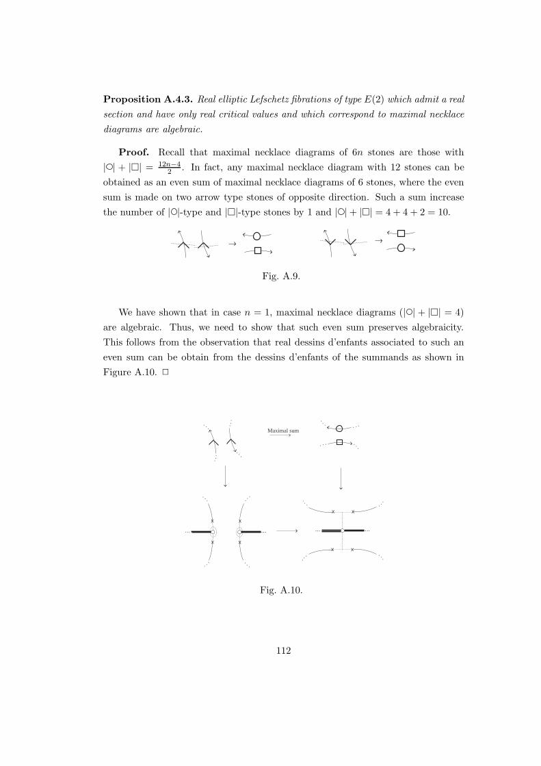
Proposition A.4.3. Real elliptic Lefschetz fibrations of type E(2) which admit a real
section and have only real critical values and which correspond to maximal necklace
diagrams are algebraic.
Proof. Recall that maximal necklace diagrams of 6n stones are those with
| | + || = 12n−42 . In fact, any maximal necklace diagram with 12 stones can be
obtained as an even sum of maximal necklace diagrams of 6 stones, where the even
sum is made on two arrow type stones of opposite direction. Such a sum increase
the number of | |-type and ||-type stones by 1 and | | + || = 4 + 4 + 2 = 10.
Fig. A.9.
We have shown that in case n = 1, maximal necklace diagrams (| | + || = 4)
are algebraic. Thus, we need to show that such even sum preserves algebraicity.
This follows from the observation that real dessins d’enfants associated to such an
even sum can be obtain from the dessins d’enfants of the summands as shown in
Figure A.10. 2
x
x
x
x
x x
xx
.. .
.. .
...
...
.. . . ..
. .... .
Maximal sum
.. . . ..
. ....
.
. ..
. ....
.
.. .
... ...... ...
Fig. A.10.
112

Example A.4.4. An example of even sum which creates maximal necklace diagram
and corresponding real dessins d’enfants are given in Figure A.11
xx
xx
xx
xx
xx
x
x
x
x
x
x
xx
x
x
xx x
x
xx
xx
xx
xx
xx
x
x
x
x
x
x
xx
x
x
xx x
x
Fig. A.11. An example of even connected sum creating a maximal necklace diagram.
113

Real dessins d’enfants of real E(1) with real sections.
xx
xx
xx
x x
xx x
xx
xx
x
xxx x
xx x
x
x
x
xx
x
x
x
x x
x x
x
x
x
xx
x
x
x
x x
x x
x x
x
xx
x
x
x
xxx
x
x
x
x
xx
x
x
x
x
xxx
x
Fig. A.12. Around necklace diagrams, the real part of the corresponding real ellipticLefschetz fibrations are shown. The dotted inner circle stands for a lift of the exceptionalsection.
114

x
x
xx
x
x
x xxx
x
x
x
x
xx
x
x
x
x
xxx
x
xx
xx
x
x
x
x
xxx
x
x
xxx
x
x
x
x
xx
x
x
Fig. A.13. Around necklace diagrams, the real part of the corresponding real ellipticLefschetz fibrations are shown. The dotted inner circle stands for a lift of the exceptionalsection.
115

vita
PERSONAL INFORMATION
Surname, Name: Salepci Nermin
Nationality: Turkish (T. C.)
Date and Place of Birth: 27 March 1976, Yapraklı
Marital Status: Single
email: [email protected]
EDUCATION
Degree Institution Year of Graduation
MS METU, Mathematics 2001
BS METU, Mathematics 1998
High School Dikmen Lisesi 1993
WORK EXPERIENCE
Year Place Enrollment
2006-2008 Universite Louis Pasteur, Mathematics ATER
1999-2005 METU, Mathematics Teaching Assistant
FOREIGN LANGUAGE
English, French
ACADEMIC VISITS
1. June 2003 - January 2004, Universite Louis Pasteur, Strasbourg, France
2. January 2004- April 2004, MSRI, Berkeley, USA
3. September 2005 -December 2005, IHP, Paris, France
4. January 2006-August 2008, Universite Louis Pasteur, Strasbourg, France
GRANTS
Throughout my thesis I have been supported partially by TUBITAK, European
Doctoral College and French Embassy in Ankara.
116


