Eur. Phys. J. B (2021) 94 :159https://doi.org/10.1140/epjb/s10051-021-00172-1

THE EUROPEANPHYSICAL JOURNAL B

Topical Review - Statistical and Nonlinear Physics

Nested sampling for materialsLivia B. Partay1,a , Gabor Csanyi2, and Noam Bernstein3

1 Department of Chemistry, University of Warwick, Coventry CV4 7AL, UK2 Department of Engineering, University of Cambridge, Trumpington Street, Cambridge CB2 1PZ, UK3 Center for Computational Materials Science, U. S. Naval Research Laboratory, Washington, DC 20375, USA

Received 4 May 2021 / Accepted 20 July 2021 / Published online 3 August 2021© The Author(s) 2021

Abstract. We review the materials science applications of the nested sampling (NS) method, which wasoriginally conceived for calculating the evidence in Bayesian inference. We describe how NS can be adaptedto sample the potential energy surface (PES) of atomistic systems, providing a straightforward approx-imation for the partition function and allowing the evaluation of thermodynamic variables at arbitrarytemperatures. After an overview of the basic method, we describe a number of extensions, including usingvariable cells for constant pressure sampling, the semi-grand-canonical approach for multicomponent sys-tems, parallelizing the algorithm, and visualizing the results. We cover the range of materials applicationsof NS from the past decade, from exploring the PES of Lennard–Jones clusters to that of multicomponentcondensed phase systems. We highlight examples how the information gained via NS promotes the under-standing of materials properties through a novel way of visualizing the PES, identifying thermodynamicallyrelevant basins, and calculating the entire pressure–temperature(–composition) phase diagram.

1 Introduction

The potential energy surface (PES) describes the inter-action energy of a system of particles as a functionof the spatial arrangement of atoms and, within theBorn–Oppenheimer approximation, contains all struc-tural and mechanical information—both microscopicand macroscopic—about the system. [1] Its global min-imum corresponds to the ground-state structure, whilethe usually numerous local minima are other stable ormetastable configurations linked to each other by tran-sition states, which determine the pathways betweenthese different structures, along with the transforma-tion mechanisms. An alternative, equilibrium statisti-cal mechanics view of the PES is given by the freeenergy of various phases, which quantifies the interplaybetween energetic factors, which favor lower potentialenergy, and entropic factors, which favor a large config-uration space volume accessible to each phase. Thosespecific regions of the PES where the number of avail-able configurations dramatically decreases as tempera-ture decreases correspond to phase transitions, such ascondensation and freezing. The description and under-standing of these properties of the PES underpin a widerange of research areas, from interpreting dynamic pro-cesses in reaction chemistry, protein folding, and study-ing supercooled liquids to understanding the micro-scopic details of phase transitions.

a e-mail: Livia.Bartok-Partay@warwick.ac.uk (corre-sponding author)

Computer simulations have become an essential toolin exploring the PES, providing both thermodynamicinformation and an atomic level insight into materi-als properties. A plethora of computational methodshave been developed, but most such techniques targetonly a particular part or aspect of the landscape, orare optimised to map only certain properties of com-plex landscapes. Global optimization methods focuson building a database of minima to find the low-est energy structure. These include basin hopping [2],genetic algorithms [3,4], minima hopping [5] and sim-ulated annealing [6] with adaptive cooling rates [7],as well as dedicated crystal structure prediction tools,such as AIRSS [8,9], USPEX [10,11], and CALYPSO[12,13]. These techniques enable the exploration ofthe hitherto unknown basins of the PES, and havealready lead to the discovery of novel phases of arange of materials [8,9,14]. However, while the dimen-sionality of the PES scales linearly with the num-ber of atoms, the available configuration space vol-ume scales exponentially with this number. It is alsocommonly thought that the number of local minimascales exponentially as well [15], which can dramat-ically increases the computational cost, rendering itimpossible to perform an exhaustive search of all poten-tial minima basins of even moderately complex sys-tems.

The physical behaviour of materials is often domi-nated by entropic effects, and the calculation of freeenergies requires sampling over vast regions of the PESinstead of concentrating only on the minima struc-tures. Temperature-accelerated dynamics [16], samples

123

159 Page 2 of 18 Eur. Phys. J. B (2021) 94 :159

Fig. 1 Temperature–enthalpy curve (purple, enthalpy decreases from left to right) of lithium modelled by the embeddedatom model (EAM) of Nichol and Ackland [27] at 14 MPa showing both the vaporisation (2450 K, – 0.3 to – 0.9 eV) andmelting (700 K, – 1.40 to – 1.45 eV) transitions. Dashed lines illustrate the difference between the series of sampling levelsfor parallel tempering (left panel), Wang–Landau sampling (middle panel), and nested sampling (right panel). In the case ofNS, these are equidistant in ln Γ (for clarity, only one out of every 20,000 iterations). The density of NS levels as a functionof enthalpy (blue, right y-axis, right panel only) shows the general increase in sampling density as enthalpy decreases,superposed with small amplitude peaks localized in the two phase transition ranges. Red arrows illustrate the directionof the sampling’s progress; purple dots are guide to the eye. The enthalpy curve was calculated with NS of 64 atoms andK = 648

rare events and umbrella sampling [17], and meta-dynamics [18] enable the evaluation of relative freeenergies. A range of methods have been specificallydeveloped to study phase transitions: Gibbs-ensembleMonte Carlo method to study the boiling curve [19],two-phase coexistence methods and the multithermal-multibaric approach [20] to determine the melting line,or thermodynamic integration and lattice-switch MonteCarlo [21] to pinpoint solid–solid transitions. Apartfrom these often being highly specific, with most ofthem optimal only for a single type of transition, if asolid phase is involved, they also require an advanceknowledge of the corresponding crystalline structures,limiting their predictive power to exploring knownphases.

Although all of the techniques mentioned above pro-vide important information about different segmentsof the landscape, we can see that gaining a broaderoverview of the entire PES with these would be a chal-lenging and highly laborious task. There are very fewtechniques that allow the unbiased sampling of largeregions of the PES without prior knowledge of sta-ble structures or estimated location of phase transi-tions. The two most widely used are parallel temper-ing [22,23] and Wang–Landau sampling [24,25]. How-ever, these methods also face general challenges, illus-trated in Fig. 1, demonstrating the location of sam-pling levels around first-order phase transitions, wherethe enthalpy of the system changes rapidly with tem-perature. Parallel tempering samples the PES at fixed

temperatures (Fig. 1, left panel). The overlap betweenthe distributions of energies and their correspondingatomic configurations at temperatures just above andjust below a phase transition is very small, vanish-ing in the thermodynamic limit, due to the entropyjump. It is well understood that this makes equili-bration of samplers that are in two different phasesespecially difficult [26]. Wang–Landau sampling (mid-dle panel) is done on energy levels constructed tobe equispaced. Although this provides a much bettersampling of first-order phase transitions, the appropri-ate sampling levels still have to be determined manu-ally.

The nested sampling (NS) scheme, introduced bySkilling [28–30], can overcome this challenge of equi-libration by automatically creating, using a single top–down pass, a series of energy levels equispaced in ln Γ,where Γ is the configuration space volume accessi-ble below each energy. As shown in the right-handpanel of Fig. 1, this means that sampling levels aremuch denser at lower energies or enthalpies, wherethey precisely sample small energy differences relevantfor low temperatures, and also slightly denser as themethod goes through each phase transition. In thiswork, we review how the nested sampling techniquecan be adapted to sample the PES of atomic systems,describe its advantages, and illustrate how thermody-namic and structural information can be extracted fromthe results, with examples from several different appli-cations.

123

Eur. Phys. J. B (2021) 94 :159 Page 3 of 18 159

2 The nested sampling method

Nested sampling was introduced by Skilling [28–30]in the field of applied probability and inference, tosample sharply peaked probability densities in high-dimensional spaces. The algorithm can provide bothposterior samples and an estimate of the Bayesian evi-dence (marginal likelihood), Z, of a model, as

Z =∫

L(x) dx (L ≥ 0), (1)

where L is the likelihood function.The NS technique has been quickly taken up in the

field of astrophysics [31–35] and gravitational wave dataanalysis [36,37], and has gradually been adapted toexplore the parameter space in a wide range of disci-plines, such as data analysis [38], signal processing [39],phylogenetics [40], and systems biology [41,42].

The above integral also naturally translates to mate-rials science problems. Sampling the 3N -dimensionalconfiguration space of a system of N particles is thehigh-dimensional space, and the likelihood is given bythe probability of microstates, which is proportionalto the Boltzmann factor. Thermodynamic quantitiesdepend on the PES through the canonical partitionfunction of the system

Z(β) =∫

e−βE(x,p) dxdp, (2)

where β is the inverse thermodynamic temperature, Eis an energy, enthalpy, or related quantity, x and p arethe positions and momenta, respectively, and the inte-gral is carried out over the microstates of the system.To relate this expression to Eq. 1, it can be written interms of an integral over E weighted by the derivativeof the cumulative density of microstates Γ(E), as

Z(β) =∫

Γ′(E)e−βEdE, (3)

up to an overall constant factor. If the energy can beseparated into a sum of a position-dependent potentialand a momentum-dependent kinetic contribution, themomentum-dependent partition function Zp(β) can befactored out, and the integrand remains unchanged ifΓ(E) and E are understood to mean only the position-dependent parts. If samples from Γ(E) are available ata set of energies Ei in decreasing order, this equationcan be approximated as

Z(β) ≈∑

i

(Γ(Ei−1) − Γ(Ei)) e−βEi , (4)

where wi = Γ(Ei−1) − Γ(Ei) is the configuration spaceweight associated with each sample. Many thermody-namic properties can be related to simple functions ofthe partition function, including the free energy (its log-arithm), internal energy (its first derivative with respect

to the inverse thermodynamic temperature), and spe-cific heat (its second derivative). Analogous approxi-mations for these quantities can be derived by analyti-cally applying the operations to each term in the sum.If the configurations corresponding to each energy xi

are available, expectation values of arbitrary position-dependent properties can also be evaluated from

〈A(β)〉 ≈ 1Z(β)

∑i

A(xi)wie−βEi , (5)

where A(x) is the value of the property for the speci-fied positions. The fundamental modelling assumptionunderlying this approximation is that samples that arewell suited to estimating the cumulative density ofstates Γ(E) are also well suited for estimating otherobservables.

Nested sampling addresses the problem of finding asuitable set of sample points and associated weightsfor estimating the above integrals. There is a largedegree of efficiency to be gained by coarsely samplingparts of phase space which contribute very little tothe overall sum, i.e., those with relatively high energy,and conversely, by refining the sampling in those—exponentially small—parts of phase space where theenergy is low.

2.1 The iterative algorithm

The basic NS algorithm applied to sampling the poten-tial energy landscape of atomistic systems is illustratedin Fig. 2. The sampling is initialised by generatinga pool of K uniformly distributed (in x space) ran-dom configurations, often referred to as the ‘live set’or ‘walkers’. These represent the “top” of the PES,the high-energy gas-like configurations, since that phaseinevitably dominates a truly uniform sampling due toits large configuration space volume. Then, the follow-ing iteration is performed, starting the loop at i = 1:

1. Record the energy of the sample with the highestenergy as Ui, and use it as the new energy limit,Ulimit ← Ui. The corresponding phase-space volumefor U < Ulimit is Γi = Γ0[K/(K + 1)]i.

2. Remove the sample with energy Ui from the pool ofthe walkers and generate a new configuration uni-formly random in the configuration space, subjectto the constraint that its energy is less than Ulimit.

3. Let i ← i + 1 and iterate from step 1.

This iteration generates a sequence of samples xi, cor-responding energies Ui = U(xi), and weights wi givenby the differences between each sample’s volume andthe volume of the next sample Γ0

([K/(K + 1)]i −

[K/(K + 1)]i+1), which together can be used to eval-

uated thermodynamic functions and other observablesusing Eqs. 4 and 5.

The NS process ensures that at each iteration, thepool of K samples is uniformly distributed in configu-ration space with energy U < Ulimit. The finite sample

123

159 Page 4 of 18 Eur. Phys. J. B (2021) 94 :159

Fig. 2 Illustration of the nested sampling algorithm, show-ing several steps of the iteration. Panels on the left-handside represent the PES (the vertical axis being the poten-tial energy, while the other two axes representing thephase-space volume). Black dots on the landscape demon-strate the members of the live set (in this illustrationK = 9) uniformly distributed in the allowed phase space—corresponding atomic configurations (assuming constantvolume sampling) are shown in the right-hand side pan-els. In the middle two panels, the samples with the highestenergy are shown by blue, with the corresponding energycontour illustrated by a dotted line

size leads to a statistical error in ln Γi , and also inthe computed observables, that is asymptotically pro-portional to 1/

√K, so any desired accuracy can be

achieved by increasing K. Note that for any given K,the sequence of energies and phase volumes convergesexponentially fast, and increasing K necessitates a newsimulation from scratch.

It is important to note the absence of the temperatureβ from the actual sampling algorithm. Even withoutexplicit dependence on the temperature, the sequence

of configurations and weights generated by NS can beused to efficiently calculate expectation values with theBoltzmann weight. Within any one phase, the low-energy regions, which are exponentially emphasized bythe Boltzmann factor, are well sampled by the NS algo-rithm’s configurations, which are exponentially concen-trated (as a function of iteration) into the shrinkinglow-energy configuration space volume. Between ther-modynamically stable phases, where the configurationspace volume decreases a lot. The high overlap betweensuccessive samples eases equilibration, allowing the pro-cess to smoothly go from the typical high-temperaturephase configuration distribution to the low-temperaturephase distribution. Thus, the expectation value of anyobservable can be calculated at an arbitrary tempera-ture during the postprocessing, simply by re-evaluatingthe partition function and expectation value with a dif-ferent β over the same sample set, obviating the needto generate a new sample set specific to each desiredtemperature. The range of accessible temperatures is,however, limited by the range of energies sampled. Asthe temperature goes down, so do the relevant energies,and as a result, any given finite length run only includesuseful information above some minimum temperature,which is proportional to the rate of change of Ulimit asa function of iteration at the end of the run.

2.2 Generating new sample configurations

The initial live set consists of randomly generated con-figurations, ensuring their uniform distribution in thephase space. But how can we practically maintain thisrequirement as the sampling progresses? As the con-figuration space shrinks exponentially with decreas-ing energy, naive rejection sampling—where uniformlydistributed random configurations are proposed, andonly accepted if their energy is below the current limitUi < Ulimit—quickly becomes impractical, becauseessentially all proposals are rejected. Instead, we ran-domly select and clone an existing configuration fromwithin the current live set, as a starting point for gener-ating the new configuration. This cloned sample is thenmoved in configuration space long enough that we cantreat it as an independent sample. A Monte Carlo pro-cedure to reproduce the target distribution, namely uni-form in configuration space below the limiting energy,simply consists of proposing moves that obey detailedbalance (i.e., are reversible) and rejecting moves thatexceed the energy maximum.

Various types of moves are needed to efficientlyexplore all of the relevant degrees of freedom, illus-trated in Fig. 3. The most obvious is the motion ofthe atoms, which can be carried out with single-atommoves, but these are efficient only if the resulting energychange can be calculated in O(1) time. This is in prin-ciple true for all short-ranged interatomic potentials,although implementations to actually carry out this cal-culation efficiently are not necessarily available. Naivemultiatom moves with sufficiently large displacementsare hard to propose, since the associated energy change

123

Eur. Phys. J. B (2021) 94 :159 Page 5 of 18 159

(a1)

(d)

(c)

(b)

(f)

(e)

(a2)

(a3) (g)

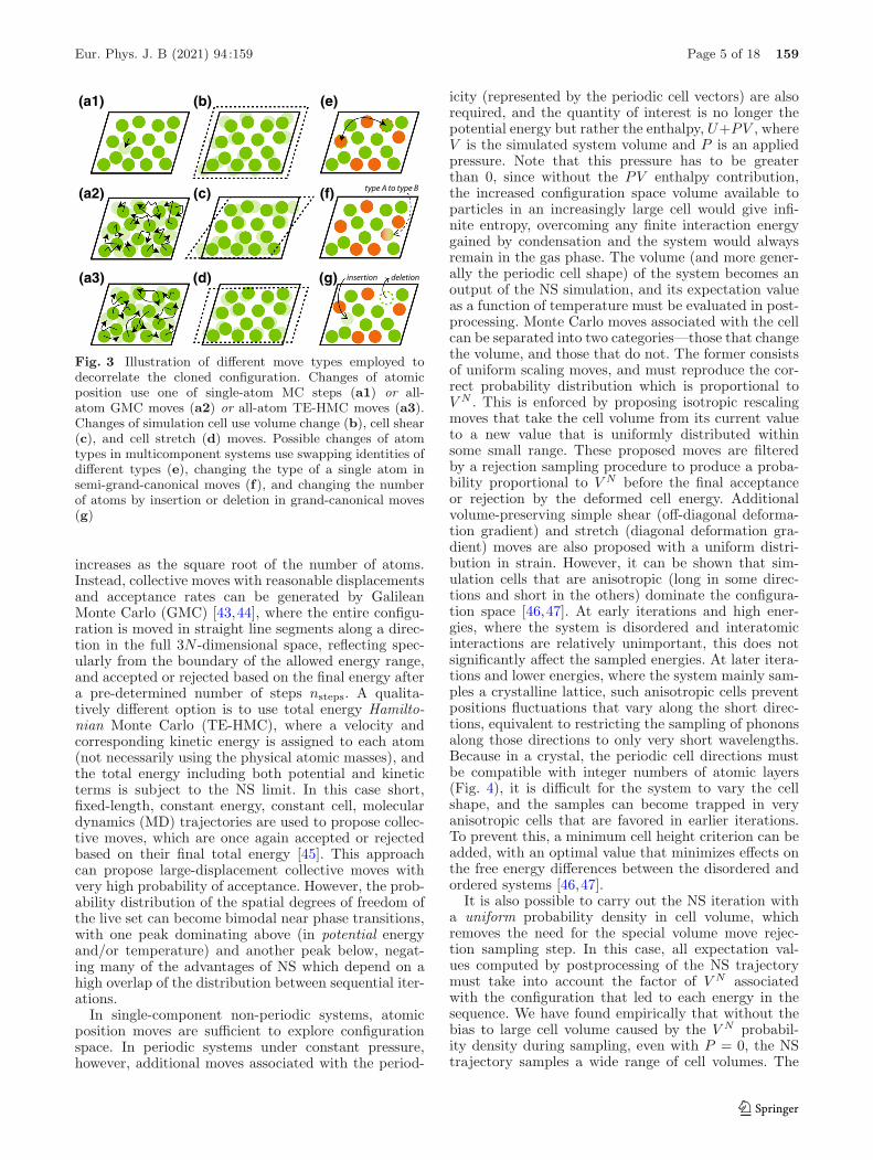
Fig. 3 Illustration of different move types employed todecorrelate the cloned configuration. Changes of atomicposition use one of single-atom MC steps (a1) or all-atom GMC moves (a2) or all-atom TE-HMC moves (a3).Changes of simulation cell use volume change (b), cell shear(c), and cell stretch (d) moves. Possible changes of atomtypes in multicomponent systems use swapping identities ofdifferent types (e), changing the type of a single atom insemi-grand-canonical moves (f), and changing the numberof atoms by insertion or deletion in grand-canonical moves(g)

increases as the square root of the number of atoms.Instead, collective moves with reasonable displacementsand acceptance rates can be generated by GalileanMonte Carlo (GMC) [43,44], where the entire configu-ration is moved in straight line segments along a direc-tion in the full 3N -dimensional space, reflecting spec-ularly from the boundary of the allowed energy range,and accepted or rejected based on the final energy aftera pre-determined number of steps nsteps. A qualita-tively different option is to use total energy Hamilto-nian Monte Carlo (TE-HMC), where a velocity andcorresponding kinetic energy is assigned to each atom(not necessarily using the physical atomic masses), andthe total energy including both potential and kineticterms is subject to the NS limit. In this case short,fixed-length, constant energy, constant cell, moleculardynamics (MD) trajectories are used to propose collec-tive moves, which are once again accepted or rejectedbased on their final total energy [45]. This approachcan propose large-displacement collective moves withvery high probability of acceptance. However, the prob-ability distribution of the spatial degrees of freedom ofthe live set can become bimodal near phase transitions,with one peak dominating above (in potential energyand/or temperature) and another peak below, negat-ing many of the advantages of NS which depend on ahigh overlap of the distribution between sequential iter-ations.

In single-component non-periodic systems, atomicposition moves are sufficient to explore configurationspace. In periodic systems under constant pressure,however, additional moves associated with the period-

icity (represented by the periodic cell vectors) are alsorequired, and the quantity of interest is no longer thepotential energy but rather the enthalpy, U+PV , whereV is the simulated system volume and P is an appliedpressure. Note that this pressure has to be greaterthan 0, since without the PV enthalpy contribution,the increased configuration space volume available toparticles in an increasingly large cell would give infi-nite entropy, overcoming any finite interaction energygained by condensation and the system would alwaysremain in the gas phase. The volume (and more gener-ally the periodic cell shape) of the system becomes anoutput of the NS simulation, and its expectation valueas a function of temperature must be evaluated in post-processing. Monte Carlo moves associated with the cellcan be separated into two categories—those that changethe volume, and those that do not. The former consistsof uniform scaling moves, and must reproduce the cor-rect probability distribution which is proportional toV N . This is enforced by proposing isotropic rescalingmoves that take the cell volume from its current valueto a new value that is uniformly distributed withinsome small range. These proposed moves are filteredby a rejection sampling procedure to produce a proba-bility proportional to V N before the final acceptanceor rejection by the deformed cell energy. Additionalvolume-preserving simple shear (off-diagonal deforma-tion gradient) and stretch (diagonal deformation gra-dient) moves are also proposed with a uniform distri-bution in strain. However, it can be shown that sim-ulation cells that are anisotropic (long in some direc-tions and short in the others) dominate the configura-tion space [46,47]. At early iterations and high ener-gies, where the system is disordered and interatomicinteractions are relatively unimportant, this does notsignificantly affect the sampled energies. At later itera-tions and lower energies, where the system mainly sam-ples a crystalline lattice, such anisotropic cells preventpositions fluctuations that vary along the short direc-tions, equivalent to restricting the sampling of phononsalong those directions to only very short wavelengths.Because in a crystal, the periodic cell directions mustbe compatible with integer numbers of atomic layers(Fig. 4), it is difficult for the system to vary the cellshape, and the samples can become trapped in veryanisotropic cells that are favored in earlier iterations.To prevent this, a minimum cell height criterion can beadded, with an optimal value that minimizes effects onthe free energy differences between the disordered andordered systems [46,47].

It is also possible to carry out the NS iteration witha uniform probability density in cell volume, whichremoves the need for the special volume move rejec-tion sampling step. In this case, all expectation val-ues computed by postprocessing of the NS trajectorymust take into account the factor of V N associatedwith the configuration that led to each energy in thesequence. We have found empirically that without thebias to large cell volume caused by the V N probabil-ity density during sampling, even with P = 0, the NStrajectory samples a wide range of cell volumes. The

123

159 Page 6 of 18 Eur. Phys. J. B (2021) 94 :159

(a) (b)

(c)

Fig. 4 Illustration of the effect of flexible simulation cell.a Demonstrates the continuous change of the cell ratiosallowed in case of disordered system; b shows the discreteset of possible cells that accommodate integer numbers oflayers, both on the 2D orthogonal example. c Shows theconvergence of heat capacity with respect of the minimumheight ratio of the simulation cell, demonstrated in case ofthe periodic system of 64 atoms modelled by the Lennard–Jones potential at p = 0.064 ε/σ3 [47,48]. Coloured rectan-gles serve as the legend, illustrating the allowed distortion in2D. The smaller the minimum height ratio, hmin, the moreflat the cell can become. The peaks at lower temperaturecorrespond to the melting transition, and this can be seenconverged for the minimum height ratio to be at least 0.65.The higher temperature peak corresponds to the vaporisa-tion and this requires 0.35 for convergence

resulting trajectories can be used to evaluate expecta-tion values at a range of pressures by adding the PVterm to the enthalpy in the postprocessing expressions.The expected distribution of volumes is Gaussian, anddeviations from this distribution in the postprocessingweights indicate that the range of volumes is not com-patible with the pressure.

For single-component systems, atomic position andcell steps are sufficient, but this is not necessarily thecase for systems with multiple chemical species. Espe-cially in solid phases and at low temperatures, it isnearly impossible for atoms to move between latticesites, even if they can vibrate about their equilibriumpositions. To speed up the exploration of chemical order(especially important for systems that undergo solid-state order-disorder transitions), one can add atomswap moves, switching the chemical species of a ran-domly selected pair of atoms, and accepting or rejectingbased on the final energy. If inter-atom correlations are

important, it may be useful to propose moves jointlyswapping the species of compact clusters of atoms, butthis has not appeared to be necessary so far. Whileatom swap moves are sufficient for constant composi-tion simulations, it is also possible to vary the composi-tion in a semi-grand-canonical (s-GC) ensemble, wherethe total number of particles is fixed, but not the num-ber of any particular chemical species [49,50]. In thiscase, the energy or enthalpy is augmented by a chemi-cal potential term

∑i niμi, where i indicates chemical

species, ni is the number of atoms of species i, andμi is its applied chemical potential. Since only relativeenergies are meaningful, the absolute chemical poten-tials are irrelevant, and only a set of Nspecies − 1 differ-ences Δμ1j sufficient to fix all chemical potentials upto an overall shift is needed. Similarly to the case ofvolume for constant pressure NS, for s-GC simulations,the composition is a quantity that evolves during theNS iteration, and must be evaluated as a function oftemperature by postprocessing. An example of such aphase diagram is given below in Sect. 3.2.

Note that conventional grand-canonical ensemblesampling has not been tried, at least for bulk systems,because it is unlikely to be efficient. If the particlenumbers of all species can vary, the cell volume wouldhave to be fixed to prevent a degeneracy with the totalparticle number. However, this would require densitychanges to be sampled entirely by changing the num-ber of particles, which is difficult to do with apprecia-ble acceptance probability in condensed systems. Sincethe number of particles is typically small, it wouldalso discretize the possible densities in ways that maybe incompatible with the material’s low-energy crystalperiodicity. Varying the number of particles of only asubset of the atom types during sampling would notsuffer from this issue, but has not yet been tested.

The MC trajectory that decorrelates a configurationinitially generated by cloning a random remaining livepoint consists of a sequence of these types of moves.Single-atom moves or single short GMC or MD trajec-tories, individual cell volume, shear, and stretch moves,and individual atom swap and s-GC moves (as appro-priate for the type of simulation) at fixed relative fre-quencies are randomly selected. Each step is acceptedif the final configuration is below the current energylimit. These steps are performed until a desired MCwalk length, typically defined in terms of the numberof energy or force evaluations (nsteps for GMC or MD,1 for all other step types), believed to be sufficient togenerate a new uniformly distributed configuration, isreached. To ensure efficient exploration, the sizes of thesteps must be adjusted during the progress of the NS.For every fixed number of iterations, a series of pilotwalks, each with only a single move type, is initiatedto determine the optimal step size. Each pilot walk isrepeated, adjusting the step size, until the acceptancerate is in a desired range, typically around 0.25–0.5. Thequantity varied for single-atom steps is the step size, forGMC, it is the size of each step in the trajectory, and forMD, it is the integration time step (the number of stepsfor the latter two is fixed). For cell steps, the quantity

123

Eur. Phys. J. B (2021) 94 :159 Page 7 of 18 159

varied is the volume or strain range. Atom swap ands-GC steps have no adjustable parameters. The result-ing configurations are discarded, so these pilot walks donot contribute to creating new uniformly sampled con-figurations. This optimization is essential for efficientsimulation, and optimal values vary substantially fordifferent phases.

2.3 Parameters and performance

The computational cost of an NS run depends in asystematic way on the parameters of the simulation.For most chemically specific interatomic potentials (asopposed to toy models), the cost is dominated by theenergy and force evaluations needed for the MC sam-pling that produces new uncorrelated samples fromcloned samples that are initially identical. The totalcost of the NS process is therefore proportional to theproduct of the cost for each evaluation, the number ofevaluations per NS iteration, and the total number ofiterations.

The choice of interatomic interaction model not onlycontrols the cost for each evaluation, but also the phys-ical or chemical meaning of the results. Typically, rel-atively fast potentials are used, but these often havetwo issues. One is that they make incorrect predictionsfor low-energy structures that have not been previouslynoticed, because they have not been used in the contextof a method that thoroughly samples the PES to calcu-late converged equilibrium properties. The other is thatparameter files made available for standard simulationcodes often fail in parts of configuration space that NSsamples, especially at early iterations and high ener-gies, because such configurations were not consideredrelevant to any real applications during development.Nevertheless, these failures can produce artifacts in NStrajectories (e.g., atoms that come too close togetherand never dissociate), and must be corrected by, forexample, smoothing or increasing core repulsion.

The number of evaluations for each new uncorrelatedsample is proportional to an overall walk length param-eter, L. This parameter needs to be large enough thateach cloned configuration becomes uncorrelated withits source, and again samples the relevant configura-tion space uniformly. If it is not, the set of configura-tions may be stuck with only configurations relevantfor high energies, and take too many iterations, or per-haps entirely fail, to find basins that are important atlow energy. Such an error can result in underestimat-ing the transition temperature, or failing to detect thetransition at all.

The size of the live set K is another important factorin the accuracy of the results, determining the reso-lution with which the PES is mapped during the sam-pling. If it is too low, there will be systematic discretiza-tion errors, as well as noise, in the configuration spacevolume estimates and any quantities derived from them.A distinct problem caused by too small a live set isthe likelihood of missing basins that are important latein the iteration process through a phenomenon called

extinction. Any basins that are separated by barriersat some energy must be found, while the NS limit-ing energy is higher than the barrier, because later thecloning and MC walk process will not be able to reachthem. However, even if there are samples in such an iso-lated basin when the limiting energy cuts it off from theother samples, there is the possibility that the numberof samples will fluctuate to 0, in which case knowledgeof that basin will be lost and cannot be rediscovered.If there are Kb samples in a basin, its fluctuations willbe of order

√Kb, relative fluctuations will be of order

1/√

Kb, and the chance to fluctuate to zero will increaseas K decreases. In the highly multimodal PES charac-teristic of materials systems, this is an important limiton the minimum necessary live set size. One approachto address this issue in bulk systems, diffusive NS, is dis-cussed at the end of this section, and others that havebeen proposed for clusters, where the problem is evenmore frequent, are mentioned in the following sectionon applications to clusters.

The number of NS iterations is set by the minimumtemperature that needs to be described, since the rangeof configurations relevant at each temperature is set bythe balance between the decreasing configuration spacevolume and the increasing Boltzmann factor as itera-tion number increases and energy decreases. For fixedminimum temperature, the amount of compression inconfiguration space is fixed, so the number of iterationsincreases linearly with the number of walkers in thelive set K. There is some evidence, as illustrated inFig. 5, that with increasing K, the minimum sufficientL decreases, and vice versa, if K is large enough toallow sampling of all the relevant basins. This may beunderstood if the distance that the cloned configura-tion needs to diffuse in configuration space decreasesas K increases, for example, if it only needs to be lostamong the neighboring configurations, rather than fullyexplore the entire available space.

The scaling of the cost with the number of atomsN is more complicated. The first, trivial contributionis due to the cost of each energy or force evaluation,which scales at least linearly (for a localized interatomicpotential) in the number of atoms. In addition, the con-figuration space volume ratio associated with a pairof phases scales with N , so that the number of iter-ations increases linearly. As a result, the overall scalingof computational cost with the number of atoms is atleast O(N2). Note also that only the increase with walklength L and the N -dependent cost for each evaluationare amenable to parallelization—costs associated withthe number of iterations are inherently sequential, andcannot be offset by adding more parallel tasks if otherlimits apply (Sect. 2.4). In practice, we find that forgood convergence, periodic solids require systems sizesof N = 32–256 atoms, walk lengths L of 100s to 1000s,and K = 500–5000 walkers. These result in 105 to 107iterations being needed to reach the global minimum attemperatures below any structural phase transitions.

It also has to be noted that using system sizes men-tioned above will inevitably cause a finite-size effect.First-order phase transitions will be smeared out in

123

159 Page 8 of 18 Eur. Phys. J. B (2021) 94 :159

L=20

64

total cost=6.19 ×108

total cost=12.3×108

total cost=24.6×108

0

0.1

0.2

0.5 0.6 0.7 0.8

total cost=49.5×108

K=320total cost=12.2×108

total cost=24.4×108

total cost=48.8×108

0.5 0.6 0.7 0.8

total cost=99.1×108

K=640

L=2064

total cost=24.7×108

total cost=49.4×108

total cost=99.1×108

0.5 0.6 0.7 0.8

total cost=198.1×108

0

0.1

0.2

0

0.1

0.2

0

0.1

0.2

0

0.1

0.2

0

0.1

0.2

0

0.1

0.2

0

0.1

0.2

0

0.1

0.2

0

0.1

0.2

0

0.1

0.2

0

0.1

0.2

Temperature (kT/eps) Temperature (kT/eps) Temperature (kT/eps)

0.5 0.6 0.7 0.8 0.5 0.6 0.7 0.8 0.5 0.6 0.7 0.8

0.5 0.6 0.7 0.8 0.5 0.6 0.7 0.8 0.5 0.6 0.7 0.8

0.5 0.6 0.7 0.8 0.5 0.6 0.7 0.8 0.5 0.6 0.7 0.8

Hea

t cap

acity

Hea

t cap

acity

Hea

t cap

acity

Hea

t cap

acity

Increasing number of walkers, K

Incr

easi

ng w

alk

leng

th, L

K=160

L=41

28L=

8256

L=16

512

Fig. 5 Constant pressure heat capacity around the melt-ing transition, calculated for the periodic system of 64 LJparticles. Black lines show the converged result; purple linesillustrate the variation of independent NS runs of the samesystem, showing an estimate for the uncertainty. The num-ber of walkers, K, is increased left to right, the length ofthe walk, L, is increased top to bottom. The total cost isthe total number of energy evaluations performed, and isconstant along diagonal panels—grey lines are guide to theeye

temperature, rather than being truly discontinuous. Inaddition, there is a systematic shift, usually underesti-mating the temperature of the vaporisation transition,and overestimating that of the melting transition. Themagnitude of this effect varies depending on the stud-ied system and pressure, but is generally between 3 and8% if using 64 atoms [51,52].

Since its introduction by Skilling, several modifica-tions and improvements have been suggested to increasethe efficiency of the sampling algorithm. A multilevelexploration of the original top–down algorithm, the dif-fusive nested sampling [53], has shown improved effi-ciency in exploring some high-dimensional functions.Introducing varying number of live points in dynamicnested sampling has shown improved efficiency in thedistribution of samples [54].

The PES of atomistic systems is often very differ-ent in its features from the parameter spaces exploredin other disciplines. Thus, these modifications to thetechnique are not always applicable, or offer only lim-ited improvement. While in typical data analysis appli-cations, a 30-dimensional function is considered to behigh dimensional, the dimensionality of the atomisticPES is at least an order of magnitude larger. A poten-tially large number of local minima structures meanthat the PES is often highly multimodal; moreover, therelative ratio of these modes is of the utmost signifi-cance as they correspond to phase transitions in thematerial. Finally, while calculating the partition func-tion is the key advantage of NS, we are rarely interestedin its value directly. Practically useful thermodynamic

information is extracted from the sampling as its firstor second derivative, which is found to converge muchfaster than the actual value of the partition function.

A conceptually very similar algorithm, the densityof states partitioning method used by Do and Wheat-ley [55–57] can be regarded as an NS with using onlya single walker which is allowed to revisit previouslyexplored higher energy states, and reducing the phase-space volume by a constant factor of two at every sam-pling level. Their calculations also used known crys-talline structures as starting configurations [58]. A fur-ther similar techniques has since been proposed, theNonequilibrium Importance Sampling of Rotskoff andVanden-Eijnden to calculate the density of states andBayes factors, using nonequilibrium trajectories [59].

2.4 Parallelization

The fact that NS relies on a live set of many con-figurations might appear to suggest that paralleliza-tion would be straightforward, but, in fact, the naivealgorithm is entirely sequential. One configuration at atime is eliminated and another is cloned, and all of thecomputational cost is in the MC trajectory to decor-relate the cloned configuration. Several modificationshave been proposed to provide for some level of paral-lelism, including discarding and cloning multiple con-figurations [60–62], moving many live points by a smallamount at each iteration [51], and combining multipleindependent NS runs [39].

One approach is to eliminate multiple configura-tions with the highest energies at each NS iteration[61,62]. In the same way that the highest energy con-figuration provides an estimate of the boundary of theK/(K + 1) fraction of configuration space volume, theNp’th highest configuration provides an estimate of the(K − (Np − 1))/(K + 1) fraction of configuration spacevolume. Since eliminating several configurations mustbe followed by creating the same number of new decor-related configurations, the computational cost of theMC walks required can be parallelized over the Np inde-pendent configurations. Overall, the fraction of config-uration space removed at each NS iteration increasesby a factor of Np, and the number of NS iterationsto achieve a certain compression decreases by a fac-tor of Np. This reduced number of iterations is com-pensated by the computational cost of each iterationincreasing by a factor of Np, but that cost can be paral-lelized over Np tasks. Unfortunately, the variance in thecomputed phase-space volume increases with the num-ber of configurations eliminated at each NS iteration(Appendix B.2.a of Ref. [48]), increasing the amountof noise and limiting the extent of parallelization usingthis method.

Another approach is to apply the MC walk not onlyto the newly cloned configuration, but also to Np − 1other randomly selected configurations, where Np is thenumber of parallel tasks [51]. This leads to fluctua-tions in the length of the MC walk each configurationexperiences between when it is cloned (and identical to

123

Eur. Phys. J. B (2021) 94 :159 Page 9 of 18 159

another configuration) and when it is eliminated (whichis the only time its position or energy affect calculatedproperties). If at each NS iteration, each of Np con-figuration experiences an MC trajectory that is L/Np

steps, the mean number of steps for eliminated config-urations remains equal to L, although the variance ofthe walk length increases (Appendix B.2.b of Ref. [48]).Each of these shorter MC trajectories can be simulatedby one of Np parallel tasks. While there are no quanti-tative results for how much this variability affects com-puted properties, it appears empirically that the effectis small, and this parallelization method is most com-monly used in NS for materials. The degree of paral-lelization is limited by the need to keep L/Np > 1, sothat at least some MC steps are taken at each itera-tion. For GMC or TE-HMC, the ratio must be largerthan the length of a single short trajectory, typically oforder 10 GMC segments or MD timesteps. Each shorttrajectory must be performed in its entirety to main-tain the coherence between steps that gives these meth-ods the ability to propose large-amplitude moves withnon-negligible acceptance probability. In practice, theratio L/Np must be kept significantly larger to preservegood load balance between the tasks and because in thehighly parallel regime (Np of order 100) parts of the pro-cess other than the MC trajectory generation becomesignificant.

A final approach to parallelizing NS is to run mul-tiple independent trajectories and combine them afterthey are complete [39]. The combination of Np inde-pendent runs with K ′ live points each is approximatelyequivalent to a single NpK

′ live point run. While thisapproach has been explored for other applications ofNS, it has not been widely used in materials. A possi-ble reason is that the multiplicity of minima in typicalmaterials systems is extremely large, and as a result, aserious problem is presented by extinction, as describedin the previous subsection. The scope for parallelism istherefore limited by the need to keep K ′ = K/Np largeenough to prevent extinction in any important min-ima. While it has not been carefully studied, it maythat the smallest K ′ that sufficiently avoids extinctionis already too computationally expensive to allow formultiple runs.

2.5 Analyzing the results

The energies, configuration space volumes, and cell vol-umes generated by NS are sufficient to carry out theweighted sum in Eq. 4 numerically to evaluate the parti-tion function. More importantly, physically meaningfulquantities such as the energy or enthalpy and its deriva-tive, the specific heat, can be computed as a functionof temperature from Z(β). Rapid changes in the energyas a function of temperature, corresponding to peaksin the specific heat, are associated with abrupt changesin structure. For bulk systems in the thermodynamiclimit, these become first-order transitions with singu-lar specific heat, approximated by sharp peaks in thefinite-size simulated systems. These peaks provide dis-

-8

-4

0

4

0 0.2

0.6

1.0

1.4

Ent

halp

y/at

om (

eps)

Tem

pera

ture

(kT

/eps

)

NS iteration

T

enthalpyT estimate

1.2×106 8×105 4×105

0 0.2 0.4 0.6 0.8 1 1.2 1.4 1.6 0

50

100

150

200

Hea

t cap

acity

/ato

m

-8

-4

0

4

Ent

halp

y/at

om (

eps)

Temperature (kT/eps)

enthalpy

heat capacity

Fig. 6 Nested sampling of the periodic system of 64 LJparticles. Top panel shows the enthalpy and the (estimatedinstantaneous) temperature as a function of the NS itera-tions. The bottom panel shows the enthalpy and the con-stant pressure heat capacity as a function of temperaturefor the same run. Shaded grey and green areas show theiteration and enthalpy ranges, respectively, where the par-tition function contribution is 10 times smaller than at thepeak for the same temperature

tinctive signatures of such transitions, and can be usedto identify transition temperatures for phase diagrams.

An example of the raw and processed output from asingle constant pressure NS simulation of the Lennard–Jones system is shown in Fig. 6. As seen in thetop panel, the enthalpy as a function of NS iterationdecreases monotonically, by construction, but its slopebecomes more negative when the system goes throughphase transitions. At each temperature a narrow rangeof iterations (and enthalpies) contributes significantlyto the weighted sum, shifting smoothly within eachphase, and jumping discontinuously between phases.The derivative of the enthalpy with respect to iteration,which is inversely proportional to ∂H

∂S = T and gives anestimate of the temperature that the current NS iter-ation will contribute to [48], decreases monotonicallyexcept for a temporary rise as the NS iteration processbegins to go through the transition energy range. Thesharp peaks in cp(T ) shown in the bottom panel coin-cide with the discontinuities in the ensemble average ofthe enthalpy, as they must, since they are calculated asanalytical derivatives of the same weighted sum.

2.6 Implementations for materials problems

One software implementation of the nested samplingand analysis algorithms discussed above is provided bypymatnest [63]. It uses python and the atomic simu-

123

159 Page 10 of 18 Eur. Phys. J. B (2021) 94 :159

lation environment (ASE) package [64] to implementthe Monte Carlo procedure and parallelization strate-gies described in the previous sections in a way thatabstracts the material-dependent energy and force cal-culations. The PES evaluations can use any ASE cal-culator, including potentials implemented in the widelyused LAMMPS MD software [65], although the com-putational cost is significant. Another python-basedimplementation, designed for non-periodic systems, isavailable [66], and forms the basis for the implementa-tion [67] of the superposition enhanced nested samplingvariant [62], discussed in more detail below.

3 Applications

3.1 Configuration space of clusters

The use of the nested sampling framework for samplingthe potential energy landscape of materials was firstdemonstrated on small Lennard–Jones clusters [68].Lennard–Jones clusters are popular test systems fornew phase-space exploration schemes, due to the lowcomputational cost of the interaction function and thelarge amount of data on their properties available inthe literature [1,2,69,70]. Nielsen also used NS to studyLJ17 [71]. Apart from calculating thermodynamic prop-erties, this also demonstrated that NS can provide abroad-brush view of the landscape, giving a helpfuloverview of the system. Visualizing the 3N -dimensionalPES is a challenging task and projecting the landscapeusing ad-hoc order parameters can be very misleading.An efficient way of overcoming this is to represent thehierarchy of known minima and transition states using adisconnectivity graph [72–74], capturing the topology ofthe entire landscape. However, disconnectivity graphsdo not include any information on the entropic contri-bution of different basins, and thus cannot provide guid-ance in understanding the thermodynamic behaviour ofthe system. NS naturally provides this missing informa-tion which can be used for more informative visualiza-tion. If distinct structures are identified and thus sam-pled configurations are sorted according to the basinthey belong to using an appropriate metric to calculatethe distance of configurations, the relative phase-spacevolume of these basins can be easily calculated: sinceconfigurations in the live set are uniformly distributedat every sampling level, the ratio of number of samplesin different basins tells us their relative volume. Analternative that does not require explicit reference tothe live set is presented in the next section. We used thisinformation to construct the energy landscape chartof several Lennard–Jones clusters [68], where basinsof minima explored by NS are shown as funnels withappropriate widths representing their phase-space vol-ume.

The example of LJ8 is shown in Fig. 7, showing theglobal minimum structure along the seven known localminima. While all of these were found, it is obvious fromthis representation that their contribution to the phase-

Fig. 7 Energy landscape chart of 8 LJ atoms forming acluster. Grey shading and numbers in red show the uncer-tainty in the phase-space volume. Reprinted with permissionfrom Fig. 7 of Ref. [68]. Copyright 2010 American ChemicalSociety

space volume is negligible compared to the main funnelleading to the global minimum, and thus, we can safelyassume them to be thermodynamically irrelevant in thiscase. Similar energy landscape charts were also used byBurkoff et al. [60] to provide a qualitative insights intothe folding process of a couple of poly-peptides, sampledby NS.

As the size of the system and thus the number of localminima increases, we cannot expect NS to explore all ofthem: since the size of the live set, K, controls the res-olution of the PES we can see, thus narrow basins willinevitably be missed. However, since narrower basinscontribute the least to the partition function, this doesnot hinder our ability to calculate thermodynamic prop-erties and give an overview of the significant structures.This has also been demonstrated studying the melt-ing behaviour of a CuPt nano-alloy [75], and studyingthe PES of small water clusters [76], using NS to findthe few thermodynamically relevant minima. This alsoshed light on the connection between the thermody-namic properties and the features of the energy land-scape: if local minima gave an overall small contribu-tion to the total partition function, a sharp “melting”peak was observed on the heat capacity curve, whilethe existence of competing structures at finite temper-ature were associated with a more gradual transition.Figure 8 illustrates the analysis of the NS results on thecluster of 13 particles modelled by the mW potential ofwater [77].

123

Eur. Phys. J. B (2021) 94 :159 Page 11 of 18 159

Fig. 8 Nested sampling of 13 mW water particles. Upperpanel shows the heat capacity curve. In the middle panel,each dot corresponds to a configuration generated dur-ing nested sampling, showing their average Q4 bond orderparameter [78] as a function of temperature and is colouredaccording to the average ring size within the cluster to helpdistinguish different basins of the PES. The bottom panelshows the relative phase-space volume ratio of global min-imum basin (purple) and the local minimum basin (red),while the grey area represents the contribution of any otherstructure to the total partition function. Temperatures cor-responding to the peaks on the heat capacity curve, indi-cating phase transitions, are shown by vertical dotted lines.Middle panel reprinted with permission from Fig. 2 of Ref.[76]. Copyright 2019 by the Royal Society of Chemistry

While in the large majority of systems, the basinswith small phase-space volume can be disregarded with-out affecting our overall understanding, there are excep-tions, especially in case of clusters. Some systems dis-play a highly frustrated PES, where high barriers dividethe landscape and the relative phase-space volumesof basins are significantly different at different energylevels. If a basin which is narrow at higher energiesbecomes the most significant at a lower energy level, wesee a corresponding low-temperature (often solid–solid)

phase transition in the system. In such cases, the NSlive set has to be large enough to ensure a high resolu-tion capable of capturing and sampling sufficiently thenarrow basin of interest. To evade the increased com-putational cost and ensure that known minima are not“lost” during the sampling, Martiniani et al. proposed amethod combining nested sampling with global optimi-sation techniques, superposition enhanced nested sam-pling [62]. In this case, sample configurations are notonly generated from existing members of the live set,but are also drawn from a pre-existing database, pro-portional to their statistical weights, calculated usingthe harmonic superposition approximation (HSA). Itsspeed-up and accuracy has been demonstrated for LJ31and LJ38, but databases miss the astronomical num-ber of high-energy local minima that would be neces-sary to counteract the inaccuracy of HSA at high ener-gies. For larger systems with broken ergodicity, suchas LJ75, even this method struggles. To overcome thedifficulty of sampling in these particular systems, thefunnel-hopping Monte Carlo [79] and nested basin sam-pling [80] approaches have been recently proposed.

3.2 Phase diagram of materials

For bulk, rather than cluster, systems, our knowledge ofthe PES is often distilled into the form of a phase dia-gram, showing the stability regions of thermodynami-cally distinct phases or structures under different con-ditions, most typically temperature, pressure, or com-position. This is crucial in both academic and indus-trial materials science applications, to be able to predictthe state and the properties of a material. However, aswe have discussed, obtaining the entire phase diagramunder a wide range of conditions is a highly laborioustask, requiring the use of multiple, conceptually differ-ent methods, and hence, it is rarely performed in anexhaustive way.

The first application of the NS technique to a bulksystem, which used a periodic supercell approximation,was done on the hard sphere solid [81], calculating thecompressibility from the partition function to locate thefluid–solid-phase transition and discussing the phase-space volume of jammed structures. The following year,Nielsen et al. performed constant pressure NS simula-tions of two Lennard–Jones clusters in a hard spherecavity, as well as a periodic LJ system in a fixed cubicbox [82].

These works were followed by an extension of NS toconstant pressure sampling in a fully flexible periodicsimulation cell, which allowed, for the first time, the cal-culation of the entire pressure–temperature phase dia-gram of a material. The first such simulations were per-formed for the Lennard–Jones potential and four EAMmodels of aluminium, as well as for the composition–temperature–pressure phase diagram of an EAM modelof the NiTi shape memory alloy, calculating the marten-sitic phase transition [51]. This work demonstrated howthe peaks in the heat capacity curve enable us to locatenot just the boiling and melting curves, but also the

123

159 Page 12 of 18 Eur. Phys. J. B (2021) 94 :159

Fig. 9 Constant pressure heat capacity curves calculatedfrom sampling performed at a range of pressures, used tolocate phase transitions and draw the pressure–temperaturephase diagram. Application to the Ercolessi–Adams EAMpotential model for aluminium [51,84]

Widom line above the critical point, and the solid–solid-phase transitions, as demonstrated in Fig. 9. Tolocate the critical point in the nested sampling calcu-lations, we drew on the results of Bruce and Wild-ing [83]: for a finite system at and below the criticalpoint, the density distribution appears bimodal (at thetemperature corresponding to the maxima of the heatcapacity peak), while above the critical point, the den-sity distribution transitions quickly becomes unimodal.We used this argument to estimate the critical pres-sure to be between the two adjacent sampling pressureswhere the modality of the distribution changes, anddemonstrated that results provided by this approachare in very good agreement with those calculated bythe Gibbs-ensemble Monte Carlo technique [51]. Simi-lar simulations of phase transitions at a single pressurewere also calculated for the mW model of water and asystem of coarse-grained bead-spring polymers [48].

Identifying different structures using suitably cho-sen order parameters enables the separation of differentbasins of the PES. As Fig. 10 shows, NS not only identi-fies the most stable structure, but provides informationon the thermodynamically relevant metastable phasesas well. Similar extensive phase diagram comparisonstudies have been performed for a range of EAM typepotentials of iron [85] and lithium [52].

It is also possible to characterize these basins with-out the need to refer to the live set, as was done for theLennard–Jones clusters in Sect. 3.1. The entire trajec-tory is converted into a graph, where each configurationis a node, and the edges are connections to its k nearestneighbors in feature space (i.e., k most similar config-urations defined from a structurally relevant similar-ity measure). The network is separated into connectedcomponents, and each component defines a basin, iden-tified by its minimum energy structure. The configu-ration space volume associated with each basin is thesum of weights associated with each sample in the con-nected component. In order of decreasing energy, onenode (sample) and all of its edges are eliminated, and

Fig. 10 Nested sampling of the Mishin EAM for alu-minium [86]. The upper panel shows a section of thetemperature–pressure phase diagram, featuring the meltingline and the phase boundaries of the three crystalline phasesidentified by NS: fcc, hcp, and bcc. The bottom panels showthe average Q6 bond order parameter [78] as a function ofenthalpy for configuration generated during nested samplingat three different pressures. Q6 order parameter for the per-fect crystalline structures are shown by horizontal dottedlines, and the phase transition temperature between hcpand bcc is marked by a vertical dashed line in the middlepanel

the new network is analyzed for connected components.If removing the highest energy node causes a basin todecompose into two or more disconnected subgraphs,those become new basins with their own volumes, andthe energy barrier between them is simply the energyof the last node that connected them. This process isrepeated until all the samples have been eliminated. Tovisualize the results, the left and right edges of eachbasin at each iteration are plotted, so that the x-axisdistance between them is proportional to the basin’svolume at the same iteration, at a y-axis position equalto the energy of that iteration. Because the range of vol-umes can be extremely large (e.g. 1096 for a 64-atom Licell), it must be scaled to be visible in a plot. Keep-ing the relative volumes of the basins at each energy incorrect proportion, scaling the overall width to a func-tion that decreases exponentially with energy leads to avisually pleasing result that conveys the rapid decreasein configuration space.

An example from an NS simulation of Li at an appliedpressure of 15 GPa with an embedded atom model

123

Eur. Phys. J. B (2021) 94 :159 Page 13 of 18 159

Fig. 11 Visualization of the potential energy landscape oflithium at P = 15 GPa described by an EAM [89]. At highenthalpy, there is no separation into different basins, and allconfigurations are associated with a single basin. The threebasins that become distinct at lower enthalpies (dashed linesindicate the enthalpy of each barrier) correspond to the hcpstructure (orange, left), fcc structure (green, center), andmixed ABAC stacking (right, blue). At each enthalpy value,the relative widths of the basins correspond to their relativeconfiguration space volumes, and the overall width is scaledto be exponential with enthalpy. The ground-state mixedstacking basin is not closed at the bottom to indicate thatwe have no data on its minimum enthalpy, although it islikely to be close to the lowest sampled value

(EAM) [52] is shown in Fig. 11, using the similaritydefined by the configuration-averaged SOAP overlap[87,88] with nmax = 8, lmax = 8, and a cut-off of threetimes the nearest-neighbor distance of 2.55 A(from theNS trajectory’s minimum energy configuration). Theraw data are somewhat noisy, with many spurious buttiny clusters, so the basins are merged if the barrierbetween them is less than 2 eV or if they containfewer than 10 samples when they split off. The visu-alization procedure identifies three remaining basins.The first to split off is the hexagonal close-packedstructure (hcp, AB stacking of close-packed layers),which persists until low enthalpy but always occupies avery small fraction of the configuration space. At onlyslightly lower enthalpy, the face centered cubic struc-ture (fcc, ABC stacking) basin splits off, occupyingapproximately half of the explored configuration spacevolume. The remaining basin constitutes the groundstate, with mixed hcp and fcc-like ABAC stacking, butthis structure coexists with fcc for about 4 eV, onlydominating at enthalpies below about −15 eV. Thecompetition between these basins leads to variationsin the observed structure as a function of tempera-ture.

An initial study of a multicomponent system des-cribed an order–disorder transition in a solid solutionbinary-LJ system [48]. The CuAu alloy has also beenrepeatedly used as a model binary system: after cal-culating the melting line [48], the entire composition–

temperature phase diagram of the CuAu binary systemwas also calculated [90], and both NS and WL usedto study the order–disorder of the occupancy of lat-tice sites, without the liquid phase being explored [91].NS was also used to determine the mean number ofhydrogen atoms trapped in the vacancies of the α-Fephase [92]. An initial fixed composition NS simulationwas used to determine the chemical potential of a sin-gle H atom within a relatively small supercell of perfectcrystal. Simulations at a range of different H concentra-tions were carried out with NS, and then combined intoa single grand-canonical partition function (for variableH atom number) using the calculated chemical poten-tial.

The semi-grand-canonical ensemble was used to sim-ulate the temperature–composition phase diagram fora machine-learning potential of the AgPd alloy [50]. Inthis case, the composition is an output observable ofthe NS simulation, as plotted in Fig. 12 for a num-ber of NS trajectories at different chemical potentialdifference values. When the trajectory goes througha phase transition with a two-phase region, in addi-tion to the discontinuity in the equilibrium structureand average energy above and below the transition, theequilibrium composition changes as well. As a result,the peak in the specific heat as a function of temper-ature is correlated with an abrupt jump in the com-position, from the value in the high-temperature phaseto that in the low-temperature phase. Finite systemsize effects broaden the transition, as seen in the fig-ure, where the change in composition as a function of Tacross the two-phase region is rapid but far from discon-tinuous. The change becomes more abrupt as the sys-tem size increases, approaching a discontinuity, jump-ing from the liquidus to the solidus, in the large systemlimit.

An important conclusion of these calculations is thatthe macroscopic behaviour of potential models canbe very different from what is expected by chemicalintuition, and thus suggested by previous calculations.Using NS has lead to the identification of previouslyunknown crystalline phases, new ground-state struc-tures, and phase transitions not anticipated before,for a significant proportion of tested potential mod-els. Since using nested sampling, the calculation ofthe phase diagram is no longer a bottleneck, the reli-ability of the chosen model can be easily establishedby performing the sampling, and thus, we can deter-mine the conditions where the model is valid, beforeit is used for a specific purpose or study. While insome cases, the newly identified structure has littleinfluence on the practical use of the model (e.g., abcc structure transforming to body-centered-tetragonalat very low temperatures [85]), in other cases, theseshed light on significant new behaviour of the model,which affects computational findings in general. Mostnotably, NS calculations on the Lennard–Jones modelled to the discovery of new global minima: dependingon the pressure and the applied cut-off distance, the LJground-state structure can be different stacking vari-ants of close packed layers [93]. Also, recent NS stud-

123

159 Page 14 of 18 Eur. Phys. J. B (2021) 94 :159

Fig. 12 Temperature–composition phase diagram forAgxPd1−x alloy using an ML interatomic potential, calcu-lated by s-GC NS (solid lines representing n(T )), fixed com-position NS (blue circles representing transition T and verti-cal bars indicating peak width), and direct two-phase coex-istence simulation for a larger system (red circle). Dottedlines indicate boundaries of experimentally observed two-phase region, and all simulation results are shifted up by200 K to facilitate comparison with experimental shape andextent of two-phase region. The s-GC NS constant Δμ n(T )curves show a gradual shift in composition as temperaturechanges, interrupted by an abrupt change in the (finite-sizebroadened) phase transition region. The left and right edgesof the lower slope parts of each curve are the high- and low-T boundaries of the two-phase coexistence region, respec-tively. The composition-dependent phase transition between1000 K and 1500 K is the solid–liquid transition, and thelow-temperature phase transition, only shown at one com-position, is a solid-phase order–disorder transition. TakenFrom Fig. 5 in Ref. [50]

ies of the hard-core double-ramp Jagla model revealeda previously unknown thermodynamically stable crys-talline phase, drawing surprising similarities to water[94].

3.3 Broader applications in materials science

While in the majority of materials applications, thermo-dynamic properties derived from the partition functionare the target calculated quantities, its absolute valuecan also be the focus of interest. For example, the par-tition function is necessary to establish the correct tem-perature dependence of spectral lines and their inten-sity. NS, as a unique tool to give access directly to thepartition function, has been used to calculate the rovi-brational quantum partition function of small moleculesof spectroscopic interest, using the path-integral for-malism [95]. This has showed that NS can be effi-

ciently used, especially at elevated temperatures and incase of larger molecules, where the direct-Boltzmann-summation technique of variationally computed rovi-brational energies becomes computationally unfeasible.

The NS algorithm has also been applied to samplethe same path through phase space as would be cov-ered in traditional coupling-parameter-based methodssuch as thermodynamic integration and perturbationapproaches, but without the need to define the couplingparameter a priori. The combined method, CouplingParameter Path Nested Sampling [96], can be used toestimate the free energy difference between two sys-tems with different potential energy functions by con-tinuously sampling favorable states from the referencesystem potential energy function to the target potentialenergy function. The case studies of a Lennard–Jonessystem at various densities and a binary fluid mixtureshowed very good agreement with previous results.

Nested Sampling has been used to sample transitionpaths between different conformations of atomistic sys-tems [97]. The space of paths is a much larger spacethan that of the configurations themselves. To makeit finite-dimensional, the paths are discretised, and thewell-established statistical mechanics of transition pathsampling (TPS) is leveraged [98]. The top panel ofFig. 13 shows a double-well toy model with just twodegrees of freedom. There are two pathways that con-nect the two local minima, and the barrier via thetop path is slightly higher. The results of the NestedTransition Path Sampling (NTPS) shows the expectedresult: at high energies, the paths are random (black);at medium energies, the short path dominates (grey),but at low energies, the longer bottom path, which hasthe lowest barrier energy, dominates (white).

The bottom panel of Fig. 13 shows the results ofNTPS applied to a Lennard–Jones cluster of 7 particlesin two dimensions. There are four transition states thatfacilitate permutational rearrangements of the ground-state structure. Depending on the temperature (1/β),the fractions of the different mechanisms that lead tosuccessful rearrangements change, as shown. The esti-mate of the same fractions just from the transition statebarrier energies is shown by dashed lines. The differencebecomes large at high temperatures, where anharmoniceffects neglected by transition state theory but includedin NS become significant.

Nested sampling has also been used for more tra-ditional Bayesian inference problems in the context ofmaterials modelling [99]. There, the task was to recon-struct the distribution of spatially varying materialproperties (Young’s modulus and Poisson ratio) fromthe observation of the displacement at a few selectedpoints of a specimen under load. Under assumptionof linear elasticity, the displacement is a linear func-tion of the stress, given fixed material properties. Sincethe stresses cannot be observed, and the displacementsas a function of the unknown material properties arehighly nonlinear, determining the material parametersis a difficult inverse problem. The use of nested sam-pling allowed rigorous model comparison by calculat-ing the Bayesian evidence. Furthermore, under realis-

123

Eur. Phys. J. B (2021) 94 :159 Page 15 of 18 159

Fig. 13 Nested transition path sampling for a modeldouble-well potential (top) and two-dimensional LJ7 (bot-tom). The inset shows the heatmap of the double-well poten-tial, with three example transition paths: a high-energy path(black), a medium-energy short path through the slightlyhigher top barrier (grey), and a low-energy longer paththrough the slightly lower bottom barrier. In the main plot,the greyscale of the paths correspond to the NS iteration(and thus also path energy). For LJ7, the graph shows thefraction of various rearrangement mechanisms as a functionof temperature (top x axis, with inverse temperature shownon the bottom x axis). The dashed lines correspond to theexpected fraction based on the barrier heights and assum-ing harmonic transition state theory. Reprinted figure withpermission from Ref. [97]. Copyright 2018 by the AmericanPhysical Society

tic regimes including boundary conditions, number ofobservations, and level of noise, the likelihood surfaceturned out to be highly multimodal. The best recon-structions were obtained by considering the mean ofthe posterior, sampling over a very diverse parameterrange, and significantly outperformed the naive esti-mate that takes the parameters corresponding to themaximum likelihood.

4 Conclusions and future directions

The nested sampling method is a powerful way of nav-igating exponentially peaked and multimodal probabil-ity distributions, when one is interested in integralsrather than just finding the highest peak. NS usesan iterative mapping and sorting algorithm to convertthe multidimensional phase-space integral into a one-dimensional integral, enabling the direct calculation ofthe partition function for materials given a potentialenergy function. In its materials science application, NSis a top–down approach, sampling the potential energysurface of the atomic system in a continuous fashionfrom high to low energy, where the sampling levelsare automatically determined in a way that naturallyadapts to changes of the phase-space volume. Its out-put can be postprocessed to compute arbitrary prop-erties at any temperature without repeating the com-putationally demanding step of generating the relevantconfiguration samples.

The practical benefit and implications of the NSresults are inherently connected to the quality of theinteraction model employed to calculate the energyof atomic configuration. Since NS thoroughly exploresthe configuration space and finds equilibrium configu-rations, it cannot be restricted to specific experimen-tally known structures if they are not also equilibriumphases of the computational potential energy model.While on one hand, this can be turned to our advantage,and used to determine the reliability and accuracy ofexisting and widely used models in reproducing desiredmacroscopic behaviour, for many materials, in partic-ular with multiple chemical species, sufficiently accu-rate and fast potential energy models are not yet avail-able. The increasing accuracy and efficiency of machine-learning interatomic potentials is a promising avenue tofulfill this need, complementing NS to make an emerg-ing and powerful tool for predicting material properties.

The unique advantage of NS has been demonstratedfor a range of atomistic systems, gaining a broad overallview of the entire PES and providing both thermody-namic and corresponding structural information, with-out any prior knowledge of potential phases or tran-sitions. This capability inspires materials calculationsfrom a new perspective, both in terms of allowing high-throughput and automated calculation of these ther-modynamic properties, and also in enabling samplingthose parts of the configuration space that are consid-ered challenging. Its success in the systems studied sofar provides motivation to explore the application of NSfor a wider range of materials problems; studying glasstransition and behaviour of disordered phases, phasetransitions of systems exhibiting medium-range order;molecular systems, from simple particles to polymersand proteins; or sampling regions around the criticalpoint where fluctuations are typically large.

Acknowledgements L.B.P. acknowledges support fromthe EPSRC through an Early Career Fellowship (EP/T000163/1). The work of N.B. was supported by the U. S. Office

123

159 Page 16 of 18 Eur. Phys. J. B (2021) 94 :159

of Naval Research through the U. S. Naval Research Lab-oratory’s core basic research program, and computer timewas provided by the U. S. Dept. of Defense HPCMPO atthe AFRL, ARL, and ERDC centers.

Data Availability Statement This manuscript has noassociated data or the data will not be deposited. [Authors’comment: The current manuscript is a review article of pre-vious works, hence no new data and results are presented.]

Open Access This article is licensed under a Creative Com-mons Attribution 4.0 International License, which permitsuse, sharing, adaptation, distribution and reproduction inany medium or format, as long as you give appropriate creditto the original author(s) and the source, provide a link tothe Creative Commons licence, and indicate if changes weremade. The images or other third party material in this arti-cle are included in the article’s Creative Commons licence,unless indicated otherwise in a credit line to the material. Ifmaterial is not included in the article’s Creative Commonslicence and your intended use is not permitted by statu-tory regulation or exceeds the permitted use, you will needto obtain permission directly from the copyright holder.To view a copy of this licence, visit http://creativecommons.org/licenses/by/4.0/.

References

1. D. Wales, Energy Landscapes (Cambridge UniversityPress, Cambridge, 2003)

2. D.J. Wales, J.P.K. Doye, Global optimization by basin-hopping and the lowest energy structures of Lennard-Jones clusters containing up to 110 atoms. J. Phys.Chem. A 101, 5111 (1997)

3. I. Rata, A.A. Shvartsburg, M. Horoi, T. Frauenheim,K.W. Siu, K.A. Jackson, Single-parent evolution algo-rithm and the optimization of Si clusters. Phys. Rev.Lett. 85, 546 (2000)

4. N.L. Abraham, M.I.J. Probert, A periodic genetic algo-rithm with real-space representation for crystal struc-ture and polymorph prediction. Phys. Rev. B 73, 224104(2006)

5. S. Goedecker, Minima hopping: an efficient searchmethod for the global minimum of the potential energysurface of complex molecular systems. J. Chem. Phys.120, 9911 (2004)

6. S. Kirkpatrick, C.D. Gelatt, M.P. Vecchi, Optimizationby simulated annealing. Science 220, 671 (1983)

7. M. Karabina, S.J. Stuart, Simulated annealing withadaptive cooling rates. J. Chem. Phys. 153, 114103(2020)

8. C.J. Pickard, R.J. Needs, High-pressure phases of silane.Phys. Rev. Lett. 97, 045504 (2006)

9. C.J. Pickard, R.J. Needs, Highly compressed ammoniaforms an ionic crystal. Nat. Mat. 7, 775 (2008)

10. A. Oganov, C. Glass, Crystal structure prediction usingevolutionary algorithms: principles and applications. J.Chem. Phys. 124, 244704 (2006)

11. C. Glass, A. Oganov, N. Hansen, Uspex—evolutionarycrystal structure prediction. Comp. Phys. Comm. 175,713 (2006)

12. Y. Wang, J. Lv, L. Zhu, Y. Ma, Crystal structure pre-diction via particle swarm optimization. Phys. Rev. B82, 094116 (2010)

13. Y. Wang, J. Lv, L. Zhu, Y. Ma, Calypso: a method forcrystal structure prediction. Comp. Phys. Comm. 183,2063 (2012)

14. Y. Ma, M. Eremets, A.R. Oganov, Y. Xie, I. Trojan,S. Medvedev, A.O. Lyakhov, M. Valle, V. Prakapenka,Transparent dense sodium. Nature 458, 182 (2009)

15. M.R. Hoare, Structure and dynamics of simple micro-clusters. Adv. Chem. Phys. 40, 49 (1979)

16. F. Montalenti, A.F. Voter, Exploiting past visits orminimum-barrier knowledge to gain further boost in thetemperature-accelerated dynamics method. J. Chem.Phys. 116, 4819 (2002)

17. B.A. Berg, T. Neuhaus, Multicanonical ensemble: a newapproach to simulate first-order phase transitions. Phys.Rev. Lett. 68, 9 (1992)

18. C. Micheletti, A. Laio, M. Parrinello, Reconstructing thedensity of states by history-dependent metadynamics.Phys. Rev. Lett. 92, 170601 (2004)

19. A. Panagiotopoulos, Direct determination of phasecoexistence properties of fluids by monte carlo simula-tion in a new ensemble. Mol. Phys. 61, 813 (1987)

20. P.M. Piaggi, M. Parrinello, Calculation of phase dia-grams in the multithermal-multibaric ensemble. J.Chem. Phys. 150, 244119 (2019)

21. A.D. Bruce, N.B. Wilding, G.J. Ackland, Free energy ofcrystalline solids: a lattice-switch monte carlo method.Phys. Rev. Lett. 79, 3002 (1997)

22. D.D. Frantz, D.L. Freemann, J.D. Doll, Reducing quasi-ergodic behavior in monte carlo simulations by j-walking: applications to atomic clusters. J. Chem. Phys.93, 2769 (1990)

23. R.H. Swendsen, J.S. Wang, Replica monte carlo simula-tion of spin-glasses. Phys. Rev. Lett. 57, 2607 (1986)

24. F. Wang, D.P. Landau, Efficient, multiple-range randomwalk algorithm to calculate the density of states. Phys.Rev. Lett. 86, 2050 (2001)

25. A.N. Morozov, S.H. Lin, Accuracy and convergence ofthe wang-landau sampling algorithm. Phys. Rev. E 76,026701 (2007)

26. E. Marinari, Optimized monte carlo methods, inAdvances in Computer Simulation: Lectures Held at theEotvos Summer School, edited by J. Kertesz and I. Kon-dor (Springer, Berlin, 1998) p. 50

27. A. Nichol, G.J. Ackland, Property trends in simple met-als: an empirical potential approach. Phys. Rev. B 93,184101 (2016)

28. J. Skilling, Bayesian inference and maximum entropymethods in science and engineering. AIP Conf. Proc.735, 395 (2004)

29. J. Skilling, Bayesian Anal. 735, 833 (2006)30. J. Skilling, Nested sampling’s convergence, AIP Conf.

Proc., 1193, 277 (2009)31. P. Mukherjee, D. Parkinson, A.R. Liddle, A nested sam-

pling algorithm for cosmological model selection. Astro-phys. J. 638, 51 (2006)

32. F. Feroz, M.P. Hobson, Multimodal nested sampling:an efficient and robust alternative to mcmc methods forastronomical data analysis. Mon. Not. R. Astron. Soc.384, 449 (2008)

123

Eur. Phys. J. B (2021) 94 :159 Page 17 of 18 159

33. F. Feroz, M.P. Hobson, M. Bridges, Multinest: an effi-cient and robust Bayesian inference tool for cosmologyand particle physics. Mon. Not. R. Astron. Soc. 398,1601 (2009)

34. A. Fowlie, W. Handley, L. Su, Nested sampling cross-checks using order statistics. MNRAS 497, 5256–5263(2020)

35. J. Buchner, Collaborative nested sampling: Big dataversus complex physical models. Astron. Soc. Pac. 131,108005 (2019)

36. F. Feroz, J. Gair, M. Hobson, E. Porter, Use of themultinest algorithm for gravitational wave data anal-ysis. J. Phys. Conf. Ser. 26, 215003 (2009)

37. J.R. Gair, F. Feroz, S. Babak, P.G.M.P. Hobson, A.Petiteau, E.K. Porter, Nested sampling as a tool for lisadata analysis. J. Phys.: Conf. Ser. 228, 012010 (2010)

38. B.J. Brewer, Computing entropies with nested sam-pling. Entropy 19, 422 (2017)

39. R.W. Henderson, P.M. Goggans, L. Cao, Combined-chain nested sampling for efficient Bayesian model com-parison. Digit. Signal Process. 70, 84 (2017)

40. P.M. Russel, B.J. Brewer, S. Klaere, R.R. Bouckaert,Model selection and parameter inference in phylogenet-ics using nested sampling. Syst. Biol. 68, 219 (2019)

41. N. Pullen, R.J. Morris, Bayesian model comparison andparameter inference in systems biology using nestedsampling. PLoS One 9, e88419 (2014)

42. J. Mikelson, M. Khammash, Likelihood-free nested sam-pling for parameter inference of biochemical reactionnetworks. PLoS Comput. Biol. 16, e1008264 (2020)

43. J. Skilling, Bayesian computation in big spaces-nestedsampling and Galilean monte carlo. AIP Conf. Proc.1443, 145 (2012)

44. M. Betancourt, Nested sampling with constrainedHamiltonian monte carlo. AIP Conf. Proc. 1305, 165(2011)

45. S. Duane, A. Kennedy, B.J. Pendleton, D. Roweth,Hybrid monte carlo. Phys. Lett. B 195, 216 (1987)

46. D. Frenkel, Simulations: the dark side. Eur. Phys. J.Plus 128, 10 (2013)

47. R.J.N. Baldock, Classical Statistical Mechanics withNested Sampling (University of Cambridge, SpringerTheses, Springer, 2017). (Ph.D. thesis)

48. R.J.N. Baldock, N. Bernstein, K.M. Salerno, L.B.Partay, G. Csanyi, Constant-pressure nested samplingwith atomistic dynamics. Phys. Rev. E 96, 43311 (2017)

49. J.G. Briano, E.D. Glandt, Statistical thermodynamicsof polydisperse fluidse. J. Chem. Phys. 80, 3335 (1984).https://doi.org/10.1063/1.447087

50. C.W. Rosenbrock, K. Gubaev, A.V. Shapeev, L.B.Partay, N. Bernstein, G. Csanyi, G.L.W. Hart, Machine-learned interatomic potentials for alloys and alloy phasediagrams. npj Comp. Mat. 7, 24 (2021)

51. R.J.N. Baldock, L.B. Partay, A.P. Bartok, M.C. Payne,G. Csanyi, Determining the pressure-temperature phasediagrams of materials. Phys. Rev. B 93, 174108 (2016)

52. J. Dorrell, L.B. Partay, Pressure-temperature phase dia-gram of lithium, predicted by embedded atom modelpotentials. J. Phys. Chem. B 124, 6015 (2020)

53. B. Brewer, L.B. Partay, G. Csanyi, Diffusive nested sam-pling. Stat. Comput. 21, 649–656 (2011)

54. E. Higson, W. Handley, M. Hobson, A. Lasenby,Dynamic nested sampling: an improved algorithm for

parameter estimation and evidence calculation. Stat.Comput. 29, 891 (2019)

55. H. Do, J.D. Hirst, R.J. Wheatley, Rapid calculation ofpartition functions and free energies of fluids. J. Chem.Phys. 135, 174105 (2011)

56. H. Do, J.D. Hirst, R.J. Wheatley, Calculation of par-tition functions and free energies of a binary mixtureusing the energy partitioning method: application tocarbon dioxide and methane. J. Phys. Chem. 116, 4535(2012)

57. H. Do, R.J. Wheatley, Density of states partitioningmethod for calculating the free energy of solids. J.Chem. Theory Comput. 9, 165 (2013)

58. H. Do, R.J. Wheatley, Reverse energy partitioning-anefficient algorithm for computing the density of states,partition functions, and free energy of solids. J. Chem.Phys. 145, 084116 (2016)

59. G.M. Rotskoff, E. Vanden-Eijnden, dagger, Dynamicalcomputation of the density of states and Bayes factorsusing nonequilibrium importance sampling. Phys. Rev.Lett. 122, 150602 (2019)

60. N.S. Burkoff, C. Varnai, S.A. Wells, D.L. Wild, Explor-ing the energy landscapes of protein folding simulationswith Bayesian computation. Biophys. J. 102, 878 (2012)

61. R.W. Henderson, P.M. Goggans, Parallelized nestedsampling. AIP Conf. Proc. 1636, 100 (2014)

62. S. Martiniani, J.D. Stevenson, D.J. Wales, D. Frenkel,Superposition enhanced nested sampling. Phys. Rev. X4, 031034 (2014)

63. N. Bernstein, R. J. N. Baldock, L. B. Partay, J. R.Kermode, T. D. Daff, A. P. Bartok, G. Csanyi,pymatnest, https://github.com/libAtoms/pymatnest(2016). Accessed June 2021

64. A.H. Larsen, J.J. Mortensen, J. Blomqvist, I.E. Castelli,R. Christensen, M. Du�lak, J. Friis, M.N. Groves, B.Hammer, C. Hargus, E.D. Hermes, P.C. Jennings, P.B.Jensen, J. Kermode, J.R. Kitchin, E.L. Kolsbjerg, J.Kubal, K. Kaasbjerg, S. Lysgaard, J.B. Maronsson, T.Maxson, T. Olsen, L. Pastewka, A. Peterson, C. Rost-gaard, J. Schiøtz, O. Schutt, M. Strange, K.S. Thyge-sen, T. Vegge, L. Vilhelmsen, M. Walter, Z. Zeng, K.W.Jacobsen, The atomic simulation environment-a pythonlibrary for working with atoms. J. Phys. Condens. Mat-ter 29, 273002 (2017)

65. S. Plimpton, Fast parallel algorithms for short-rangemolecular dynamics. J. Comput. Phys. 117, 1 (1995)

66. S. Martiniani, J. Stevenson, https://github.com/js850/nested_sampling. Accessed Dec 2014

67. S. Martiniani, https://github.com/smcantab/sens.Accessed Dec 2014

68. L.B. Partay, A.P. Bartok, G. Csanyi, Efficient samplingof atomic configurational spaces. J. Phys. Chem. B 114,10502 (2010)

69. J.P.K. Doye, D.J. Wales, M.A. Miller, Thermodynamicsand the global optimization of Lennard-jones clusters.J. Chem. Phys. 109, 8143 (1998)

70. P.A. Frantsuzov, V.A. Mandelshtam, Size-temperaturephase diagram for small Lennard-jones clusters. Phys.Rev. E 72, 037102 (2005)

71. S.O. Nielsen, Nested sampling in the canonical ensem-ble: direct calculation of the partition function from nvttrajectories. J. Chem. Phys. 139, 124104 (2013)

123

159 Page 18 of 18 Eur. Phys. J. B (2021) 94 :159

72. O.M. Becker, M. Karplus, The topology of multidimen-sional potential energy surfaces: theory and applicationto peptide structure and kinetics. J. Chem. Phys. 106,1495 (1997)

73. D.J. Wales, M.A. Miller, T.R. Walsh, Archetypal energylandscapes. Nature 394, 758 (1998)

74. D.J. Wales, T.V. Bogdan, Potential energy and freeenergy landscapes. J. Phys. Chem. B 110, 20765 (2006)

75. K. Rossi, L. Partay, G. Csanyi, F. Baletto, Thermody-namics of cupt nanoalloys. Sci. Rep. 8, 9150 (2018)

76. J. Dorrell, L.B. Partay, Thermodynamics and the poten-tial energy landscape: case study of small water clusters.Phys. Chem. Chem. Phys. 21, 7305 (2019)

77. V. Molinero, E.B. Moore, Water modeled as an inter-mediate element between carbon and silicon. J. Phys.Chem. B. 113, 4008 (2009)

78. P.J. Steinhardt, D.R. Nelson, M. Ronchetti, Bond ori-entational order in liquids and glasses. Phys. Rev. B 28,784 (1983)

79. J.A. Finkler, S. Goedecker, Funnel hopping monte carlo:an efficient method to overcome broken ergodicity. J.Chem. Phys. 152, 164106 (2020)

80. M. Griffiths, D.J. Wales, Nested basin-sampling. J.Chem. Theory Comput. 15, 6865 (2019)

81. L.B. Partay, A.P. Bartok, G. Csanyi, Nested samplingfor materials: the case of hard spheres. Phys. Rev. E 89,022302 (2014)

82. B.A. Wilson, L.D. Gelb, S.O. Nielsen, Nested sam-pling of isobaric phase space for the direct evaluationof the isothermal-isobaric partition function of atomicsystems. J. Chem. Phys. 143, 154108 (2015)

83. A.D. Bruce, N.B. Wilding, Phys. Rev. Lett. 68, 193(1992)

84. F. Ercolessi, J.B. Adams, Interatomic potentials fromfirst-principles calculations: the force-matching method.Europhys. Lett. 26, 583 (1994)

85. L.B. Partay, On the performance of interatomic poten-tial models of iron: comparison of the phase diagrams.Comput. Mater. Sci 149, 153 (2018)

86. Y. Mishin, D. Farkas, M.J. Mehl, D.A. Papaconstan-topoulos, Interatomic potentials for monoatomic metalsfrom experimental data and ab initio calculations. Phys.Rev. B 59, 3393 (1999)

87. S. De, A.P. Bartok, G. Csanyi, M. Ceriotti, Compar-ing molecules and solids across structural and alchemi-cal space. Phys. Chem. Chem. Phys. 18, 13754 (2016).https://doi.org/10.1039/C6CP00415F

88. J. Mavracic, F.C. Mocanu, V.L. Deringer, G. Csanyi,S.R. Elliott, Similarity between amorphous and crys-talline phases: the case of TiO2. J. Chem. Phys. Lett.9, 2985 (2018). https://doi.org/10.1021/acs.jpclett.8b01067

89. D.K. Belashchenko, Impact compression of alkali met-als: computer-aided simulation. High Temp. 51, 626(2013)

90. A. Gola, L. Pastewka, Embedded atom method poten-tial for studying mechanical properties of binary cu-aualloys. Model. Simul. Mater. Sci. Eng. 26, 055006 (2018)

91. C. Sutton, S.V. Levchenko, First-principles atomisticthermodynamics and configurational entropy. Front.Chem. 8, 757 (2020)

92. E.R.M. Davidson, T. Daff, G. Csanyi, M.W. Finnis,Grand canonical approach to modeling hydrogen trap-ping at vacancies in α-fe. Phys. Rev. Mater. 4, 063804(2020)

93. L.B. Partay, C. Ortner, A.P. Bartok, C.J. Pickard, G.Csanyi, Polytypism in the ground state structure of theLennard-jonesium. Phys. Chem. Chem. Phys. 19, 19369(2017)

94. A. P. Bartok, G. Hantal, L. B. Partay, Insight into liquidpolymorphism from the complex phase behavior of asimple model. Phys. Rev. Lett. 127, 015701 (2021)

95. B. Szekeres, L.B. Partay, E. Matyus, Direct computa-tion of the quantum partition function by path-integralnested sampling. J. Chem. Theory Comput. 14, 4353(2018)

96. L.D.G. Blake, A. Wilson, A.T. Nasrabadi, S.O. Nielsen,Computing free energies using nested sampling-basedapproaches. Mol. Sim. 44, 1108 (2018)

97. P.G. Bolhuis, G. Csanyi, Nested transition path sam-pling. Phys. Rev. Lett. 120, 250601 (2018)

98. C. Dellago, P. G. Bolhuis, P. L. Geissler, Transition pathsampling, in Advances in Chemical Physics, Vol.23,edited by I. Prigogine and S. A. Rice ( John Wiley ‘I&’Sons, 2002) Chap. 1, pp. 1–78

99. A. Vigliotti, G. Csanyi, V. Deshpande, Bayesian infer-ence of the spatial distributions of material properties.J. Mech. Phys. Solids 1188, 74 (2018)

123