Network Bandwidth Utilization Forecast Model on High Bandwidth Network

Wucherl (William) Yoo, Alex Sim

Lawrence Berkeley National Laboratory, Berkeley, CA, USA

Disclaimers

This document was prepared as an account of work sponsored by the United States Government. While this document is believed to contain correct information, neither the United States Government nor any agency thereof, nor the Regents of the University of California, nor any of their employees, makes any warranty, express or implied, or assumes any legal responsibility for the accuracy, completeness, or usefulness of any information, apparatus, product, or process disclosed, or represents that its use would not infringe privately owned rights. Reference herein to any specific commercial product, process, or service by its trade name, trademark, manufacturer, or otherwise, does not necessarily constitute or imply its endorsement, recommendation, or favoring by the United States Government or any agency thereof, or the Regents of the University of California. The views and opinions of authors expressed herein do not necessarily state or reflect those of the United States Government or any agency thereof or the Regents of the University of California.

Network Bandwidth Utilization Forecast Model on High Bandwidth Network

W ucherl (W illiam ) Yoo A lex SimLawrence Berkeley National Laboratory Lawrence Berkeley National Laboratory

Email: wyoo@lbl.gov Email: asim@lbl.gov

Abstract—With the increasing number of geographically dis­tributed scientific collaborations and the scale of the data size growth, it has become more challenging for users to achieve the best possible network performance on a shared network. We have developed a forecast model to predict expected bandwidth utilization for high-bandwidth wide area network. The forecast model can improve the efficiency of resource utilization and scheduling data movements on high-bandwidth network to accommodate ever increasing data volume for large-scale scientific data applications. Univariate model is developed with STL and ARIMA on SNMP path utilization data. Compared with traditional approach such as Box-Jenkins methodology, our forecast model reduces computation time by 83.2%. It also shows resilience against abrupt network usage change. The accuracy of the forecast model is within the standard deviation of the monitored measurements.

Keywords—Forecasting, Network, Time series analysis

I . IN TRO DUCTIO N

With advances in large scale experiments and simulations, the data volume of scientific applications has rapidly grown. Even with advances in network technology, it has become more challenging to efficiently coordinate network resources and to achieve best possible network performance on a shared network. It is also challenging to build a forecast model for network bandwidth utilization with accurate and fine­grained forecast due to computational complexities. To support efficient resource management and scheduling data movement for ever increasing data volume in extreme-scale scientific applications, we have developed an analytical model in order to characterize and forecast1 bandwidth utilization on high-speed wide area network (WAN). This forecast model can improve the efficiency of network bandwidth resource utilization. In addition, it can help to find efficient resource scheduling and path finding for data transfers.

The forecast model can improve the efficiency of network bandwidth resource utilization. In addition, it can help efficient resource scheduling and path finding for data transfers. The goal of this paper is to model the network bandwidth utilization between two sites to support data flow timing and parameter decisions as well as network topology or link planning. Our

Tn general, forecast is a subset of prediction. In this paper, we explicitly make a distinction between forecast and prediction. We use forecast as estimation of future values based on the analytical model built from past observations. We use prediction as estimation of values based on analytical model when forecast is inappropriate to use, e.g., 1) forecast of network traffic of tomorrow based on time series model of past observations 2 ) prediction of present network traffic using observations from packet probes.

modeling efforts can help systematic data transfer parameter decisions without over/under-provision. One of our previous works proposed a network reservation framework to provide guaranteed bandwidth on ESNet [5], Our forecast model can complement this type of reservation system or a system to select alternate paths for large data transfer.

It is better for the model to be computationally efficient and comparably accurate in order to forecast multiple paths of users’ interests. We select a size of an appropriate training set that shows relatively accurate forecast error with manageable computational requirement. In addition, we have studied the effect of variability of the bandwidth usage on the forecast accuracy and the appropriate threshold to make our model resilient against the abrupt usage change.

The experimental data on SNMP link utilization has been collected by ESnet [1] in 2013 and 2014 on each router. Our experiments use SNMP data from 6 directional paths connecting a pair of large data facilities described in Sec. IV-A. The SNMP data consists of the size of bandwidth utilization and time-scale as 30 seconds interval. The maximum size of bandwidth utilization is extracted at each interval from the routers in each path, which represents bandwidth utilization in the path. It is well known that Internet traffic has cyclic self-similarity in daily interval. We show this daily seasonality is also present in the SNMP data in Sec. IV-B. Our analysis focuses on the traffic for large-scale scientific data movement instead of Internet traffic.

We have developed the forecast model as a univariate time series model. The first step is to remove the seasonality in the measurement data, and we use Seasonal Decomposition of Time Series by Loess (STL) [9], STL decomposes the SNMP data into the time series of seasonality, trend and remainder. We seasonally adjust the SNMP data by deducting seasonality component. Then, we use AutoRegressive Integrated Moving Average (ARIMA) on the seasonally adjusted time series. The orders of ARIMA model are selected in an automated mechanism based on the assumption of stationary time series about the SNMP data. We have observed that there is no significant changes in the average bandwidth utilization in the training dataset window (up to 8 weeks) throughout 2013 and 2014. We show that our assumption is appropriate for the SNMP data in Sec. IV-C. Our forecast model reduces computation time for forecast by 83.2% compared to the traditional approach such as Box-Jenkins methodology [7] [8] to find the best fit forecast model using ARIMA. In addition, our model shows more resilience against abrupt network usage change.

The rest of paper is organized as follows. Sec. II presents related work. Sec. Ill demonstrates the model design and implementation. Sec. IV presents experimental evaluation of the forecast model, and Sec. V concludes.

II. R e l a t e d W o r k

The studies have shown self-similarity of network traffic in LAN [21], WAN [26], and World Wide Web [12], The self­similarity of network traffic allows to use past history to fore­cast near-term future. Qiao et al. [28] presented an empirical study of the forecast error on different time-scales, showing that the forecast error does not monotonically decrease with smoothing for larger time-scale.

Benson el al. [6] studied network traffic patterns in data centers using SNMP data. Yin el al. [35] proposed a mecha­nism to predict application-layer data throughput. Balman et al. [5] proposed a network reservation framework to provide guaranteed bandwidth. Our forecast model complements these works by providing traffic forecast information.

Available bandwidth can be estimated by sending probe packets as proposed from measurement tools: Pathload [18], pathChirp [29], IGI [16], and Spruce [34], Shriram et al. [32] conducted a comparison study available bandwidth estimation from various measurement tools in network simulator (ns2) [2], Croce et al. [11] proposed bandwidth estimation techniques from large-scale distributed systems. Aceto et al. [3] proposed end-to-end available bandwidth measurement infrastructure. Our forecast model focuses on the prediction of available bandwidth using passive measurements from routers instead of estimation from probing packets.

Several prediction models of TCP data transfers have been proposed. Throughput prediction models were proposed for large TCP transfers [14] [23]. Mirza et al. [24] used a machine learning mechanism to predict TCP throughput. While these works are restricted to predict TCP data transfers, our forecast model forecasts aggregated network throughput for a network path.

Several models have been proposed to forecast network traffic. Sang et al. [30] proposed short-term (a few minutes) forecast model using ARMA with 1 sec time-scale data. Papagiannaki et al. [25] proposed long-term (1 year) forecast model of Internet backbone traffic using ARIMA with 1 week time-scale data. Krithikaivasan et al. [19] proposed mid-term (1 day) forecast model using ARCH model with 15 minute time- scale data. Our model focuses on mid-term (1 day) forecast of the bandwidth utilization using 30 second time-scale data. Since the number of forecast points ( ^ dthrPa\TmR?IiiRecast) is order of magnitude larger than these models, our forecast model requires more computation and accuracy than these proposed models. Our model overcame these challenges by seasonal adjustment and stationary assumption, which were not discussed in these models.

III. M o d e l D e v e l o p m e n t

We have developed the forecast model as a univariate time series model. A forecast model estimates the future values using the observed SNMP data up to time n (x i; x 2, • • • , x n). The forecast of h steps ahead is denoted as x n {h) at time

n + h. When the observed value (xn+h) is available at time n + h, we calculate the forecast error denoting en (h) as:

en (h) = x n+h - x n (h) (1)

A. Logit Transformation

The theoretical maximum value of possible traffic size of the SNMP is 1010 bits and the minimum value is 0 bit within one second in 100G bit/second bandwidth of the current ESnet. As the SNMP data is collected in every 30 second interval, the traffic size per 30 second unit time is normalized by dividing by 30. Logit transformation is applied to the SNMP data x to set the lower and upper bounds based on these limits. Time series data x containing n observations is transformed to time series data y with lower bound a and upper bound b (1010 bit/second) as denoted in Eq. 2 The lower bound a isapproximated to 1 bit/second instead of 0 bit/second. Whilethere are very few cases observed when no transfer occurs, approximating to 1 bit/second is ignorable in the lOOGbps network.

x = time series x t = x i, X2 • • • , x n y = time series y t = y i, y 2 ■ ■ ■ ,y n

y = l o g i t ( x ) = l o g ( ^ ) (2)b — x

B. Seasonal Adjustment

After the logit transformation defined in Eq.2, the trans­formed SNMP data y is seasonally adjusted. Removing sea­sonal components from the time series allows analysis of the non-seasonal trend of the time series. This is essential to build forecast model that can project the trend and the seasonality of past history to future values. We use Seasonal Decomposition of Time Series by Loess (STL) [9] for this seasonal adjustment. STL decomposes the logit transformed SNMP data into the components of seasonality S , trend T , and remainder R as denoted in Eq. 3.

y = yt = St + Tt + R t (3)

STL applies a sequence of smoothing from Loess (Locally Weighted Regression Litting) [10]. This smoothing sequence progressively refines and improves the estimates of the sea­sonal and trend components. There exist several parameters to derive the STL model. The seasonal cycle is evaluated with possible choices such as minute, hour, day and week. The smoothing windows for the seasonality (n s) for trend (n t) are evaluated with different values. After the decomposition, we seasonally adjust SNMP data by deducting seasonality component denoted as yt = y t t = y t — S t = Tt + R t .

After the decomposition, we seasonally adjust SNMP data by deducting seasonality component denoted in Eq. 4.

V = y d = Vt - S t = T t + R t (4)

C. Bandwidth Utilization Prediction

The forecast model is developed by using AutoRegressive Integrated Moving Average (ARIMA) on the seasonally ad­justed time series, yt. ARIMA model consists of the orders of autoregressive process (p), the number of differences (d), and

the number of moving average (</). The orders of ARIMA model (p,d,q) are selected in an automated mechanism as follows. First, the stationarity of the time series is confirmed by KPSS test [20], When the stationary is confirmed, the order of differences d is selected as 0. Otherwise, d is selected as 1, which is enough to make the non-stationary time series to stationary in the experiments. We use Akaike’s Information Criterion (AIC) [4] to automatically select the modeling parameters as shown in the Box-Jenkins methodology [7] [8], AIC represents the sum of the maximum log likelihood for the estimation and the penalty from the orders of selected model. This combination allows simpler models with less numbers of orders unless the possible model shows severely low likelihood for the estimation. We calculate AIC with different combinations of p and q incrementing from 1 until the sum of p and q reaches to a certain maximum value. The model choice from AIC converges and is asymptotically equivalent to that of cross-validation [33] [31], The best model with p and q is chosen with the least value of AIC.2 In our case, the maximum sum of p and q is 10, and this is the smallest size that selects the modeling parameters result in reasonably accurate forecast from the experimental data.

After the the orders of the ARIMA model are selected, we fit the model with the seasonally adjusted time series (y iz, t/2 z, ••• ■ n„f ) and the training set of n observed data ( x i , x 2, * * * . -I', ,). The ARIMA model fitting is to estimate the parameters with the orders of autoregressive process and moving average process (after the orders of differencing if d > 0). The forecast of h time steps ahead is computed from the fitted model (yhO- Then, the seasonality component is added to these forecast values (yh) as in Eq 5. The seasonality forecast (Sji+i, S n+2, • • • , S n+h) can be estimated by simply repeating cyclic period in the decomposed seasonal component (S i, S 2, ■ ■ ■ , S n).

Vh = j//i/ T Sn+/t (5)

IV. E x p e r i m e n t a l R e s u l t s

A. Experimental Setup

Table I describes 6 directional paths used in the experi­ments.3 These paths connect two sites on ESnet in the US. Each path consists of 6 or 7 links connected with the routers in the path. PID is the path identification and will be used to distinguish the paths. We constructed the bandwidth utilization time series data by selecting the maximum value on a link in each path, for a given data collection interval. The experiments were conducted on a machine with 8-core CPU, AMD Opteron 6128 and 64 GB memory. To reduce overall execution time, we parallelized the computational tasks of parameter searching, fitting and calculating the forecast error.

The resolution of SNMP data can be decreased by 30 second time unit into larger scales and aggregating the traffic size, e.g., aggregating and normalizing the traffic into 1 minute, 5 minutes, 10 minutes, 30 minute, 1 hour, or 1 day time unit. As decreasing resolution of network traffic results in reducing the variances of the traffic, it can show less forecast error [28], It also leads to less computation time due to the decreased data size with lower resolution. However, we did not decrease the resolution of the SNMP data since it could forecast the most fine-grained level from the given the SNMP data. The forecast error with decreasing resolution showed better accuracy by sacrificing the granularity of the forecast, which was confirmed in our experiments.4

TABLE I: Description of Paths.

PID Source Destination # of I.inks

PI N E R S C A N L 7P2 A N L N E R S C 7P3 N E R S C O R N L 7

P4 O R N L N E R S C 7P5 A N L O R N L 6

P6 O R N L A N L 6Then, these forecast values are converted to the original scale using the reverse logit transformation as in Eq. 6.

x h = ( b - i exp (yh)1 + e x p (yh ) (6)

We evaluate the forecast error by a cross-validation mecha­nism for time series data proposed by Hijorth [15], The original mechanism by Hijorth computes a weighted sum of one- step-ahead forecasts by rolling the origin when more data is available. Similarly, we compute the average forecast error for 1 week by forecasting one target day (h = 1, • • • , 2880) and rolling 6 more days. We compare this cross-validation results of the forecast errors as Root Mean Squared Error (RMSE) in Sec. IV, where RMSE is calculated with R M S E (h ) =

VrE1 n|,:))2-2AIC is combined with the positive value of penalty from the orders and

negative log-likelihood.

Fig. 1 shows the plots of bandwidth utilization of the paths in Table I from Feb. 10, 00:00:00, GMT 2014 to Feb. 16, 23:59:30, GMT 2014. 5 We used the SNMP data during this time period as test set, and evaluated the forecast error using cross-validation. We computed the forecast error as Root Mean Squared Error (RMSE) from n observations (x \. x 2, • • • , x n) based on the Eq. 1. After deriving forecast values for the first day of the test set ( x \ . • • • , f 28so), the forecast error for thefirst target day R M S E ( h day i) = R M S E (h ) was computed. The forecast error for the second target day R M S E ( h day2) = M A E { h + h) was computed by adding the observations from the first target day to the previous training set (au, x 2, • • • , x n , x n+ i , x n+2, • • • , x n+h). This processes were repeated for the next 5 target days from the third target day. Then, the average of forecast errors for the 7 target days was the forecast error for the test set.

3We anonymize specific site names on a path for the data policy.4 This paper does not include the result from decreasing resolution.5We use Greenwich Mean Time (GMT) to resolve ambiguity in the

transition time between PST and PDT. The date and the time are used in this paper in GMT.

02/10 02/11 02/12 02/13 02/14 02/15 02/16 02/16 02/10 02/11 02/12 02/13 02/14 02/15 02/16 02/16 02/10 02/11 02/12 02/13 02/14 02/15 02/16 02/16

(a) PI (b) P2 (c) P3

02/10 02/11 02/12 02/13 02/14 02/15 02/16 02/16 02/10 02/11 02/12 02/13 02/14 02/15 02/16 02/16 02/10 02/11 02/12 02/13 02/14 02/15 02/16 02/16

(d) P4 (e) P5 (f) P6

Fig. 1: Bandwidth Utilization Graphs for Experimental Paths: The size of traffic is shown in vertical axis as bit/s. The horizontal axis shows the time from Feb. 10, 00:00:00, GMT 2014 to Feb. 16, 23:59:30, GMT 2014.

B. Seasonality Analysis

Fig. 2 shows the seasonally adjusted SNMP data by STL. The STL model was derived by using the parameters described in Sec. III-B. The seasonal cycle was evaluated with possible cyclic periods such as minute, hour, day and week. The smoothing parameter for the seasonality (ns) was evaluated with possible values such as the same value with np or multiples or inverse multiples of np. The smoothing parameter for trend n t was also evaluated with different values. With larger n t, the Interquartile Range (IQR) of the trend component got smaller. This is because smoothing from Loess [10] of the trend component gets smoother with larger n t, and this result is increasing IQR of the remainder component.

Different values of seasonality smoothing window (n s) showed the similar forecast accuracy. The IQR of the seasonal component did not change with different n s . In addition, trend smoothing window (n t ) changed the shape of trend, but did not change forecast accuracy. As a result, we selected n s and n t as the same as n s . While the shape and IQR were changed with different n t , the forecast error was still similar. This suggests

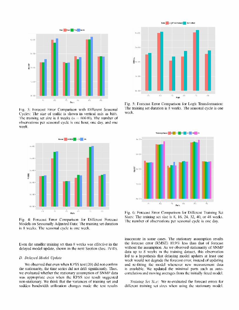
that the ARIMA is more crucial component than STL in our forecast modeling. However, fitting with STL is essential since it removes seasonal component from the original time series. Using the Seasonal ARIMA or using the ARIMA without STL appeared to be another possible choice, however computation time of the modeling these choices took too long to conduct the experiments. Only after seasonal adjustment, the computation time of the ARIMA modeling was viable. Fig. 3 shows the forecast errors when using different seasonal cycles. It is well known that Internet traffic has cyclic self-similarity in daily interval. The average forecast error (RMSE) with daily seasonality was 4.9% better than that of weekly seasonality and 2.8% better than that of hourly seasonality. This result shows that SNMP data has stronger daily self-similarity than hourly and weekly periods, similar to the Internet traffic. The average of Hurst parameters [12] from P I to P6 were 0.92, 0.94, 0.93, 0.89, 0.94, and 0.87 respectively, which confirms the self­similarity. While the remainder of STL decomposition did not pass the Ljung-Box test [22] to check whether autocorrelation still exists, which led us to use ARIMA to remove existing autocorrelation from the seasonally adjusted time series.

\ /-A ,y \/ \ / \ f \/ ^ H / \

v

tim e tim e time

(d) P4 (e) P5 (f) P6

Fig. 2: Seasonally Adjusted Components: The top plot in each graph is from the raw SNMP measurement data. The second plot is for the seasonal component. The third plot is for the trend component. The bottom plot is for the remainder. The horizontal axis shows the time as days and the duration is 8 weeks from Jan. 20, 00:00:00, GMT 2014 to Feb. 9, 23:59:30, GMT 2014.

C. Bandwidth Utilization Prediction

We compared possible modeling choices including param­eter selections. The model was developed based on the Box- Jenkins methodology [7], using ARIMA on seasonally adjusted SNMP data by STL. The orders of ARIMA model (p,d,q) were selected in the automated mechanism in Sec. III-C. After fitting the forecast model with the selected parameters, Ljung-Box test was conducted to check whether the overall residuals are similar to the white noise, and the residuals of the forecast model passed the test.

Forecast Methodology: We tested the possible forecast methods on seasonally adjusted time series data by STL. Fig. 4 illustrates the comparison of forecast errors for different forecast models, ARIMA, Exponential smoothing state space model (ETS) [17] and Random Walk (RW) [7], The forecast error of ARIMA is the lowest, which led us to use ARIMA in the forecast model.

Logit Transformation: Fig. 5 shows the forecast errors for the logit transfonned data as in Eq. 6, compared to the unmodified data. The forecast errors were derived from the forecast models using STL and ARIMA described in Sec. III-B and Sec. III-C. The forecast error (RMSE) after the logit transfonnation was consistently more accurate for each path. The average forecast error was 8.5% better with the logit transfonnation than without the logit transfonnation. This is because the logit transfonnation sets the lower and upper bounds in the modeling and fitting procedures, which helps reduce the potential under-estimation and over-estimation from the forecast.

Training Set Size: Fig. 6 shows the forecast enors for different sizes of training sets. Although the forecast accuracy was the best with 16 weeks, this was marginally better than other training set sizes. Since smaller training set required less computational resources, we used 8 weeks of training set size in the following experiments. This shows that increasing the training set size does not guarantee better forecast accuracy.

D ata | Logit Transform ed Unmodified

freq Hour Day W eek

Path

Fig. 3: Forecast Error Comparison with Different Seasonal Cycles: The size of traffic is shown in vertical axis as bit/s. The training set size is 8 weeks (n = 80640). The number of observations per seasonal cycle is one hour, one day, and one week.

Model A R I M A E T S RW

Path

Fig. 4: Forecast Error Comparison for Different Forecast Models on Seasonally Adjusted Data: The training set durationis 8 weeks. The seasonal cycle is one week.

Even the smaller training set than 8 weeks was effective in the delayed model update, shown in the next Section (Sec. IV-D).

D. Delayed Model Update

We observed that even when KPSS test [20] did not confirm the stationarity, the time series did not drift significantly. Thus, we evaluated whether the stationary assumption of SNMP data was appropriate even when the KPSS test result suggested non-stationary. We think that the variances of training set and sudden bandwidth utilization changes made the test results

P1 P 2 P 3 P 4 P 5 P 6Path

Fig. 5: Forecast Error Comparison for Logit Transfonnation: The training set duration is 8 weeks. The seasonal cycle is one week.

T rain ingW eeks | 8 ̂ 1 6 ̂ 2 4 ^ 3 2 ^ 4 0 48

Path

Fig. 6: Forecast E nor Comparison for Different Training Set Sizes: The training set size is 8, 16, 24, 32, 40, or 48 weeks. The number of observations per seasonal cycle is one day.

inaccurate in some cases. The stationary assumption results the forecast enor (RMSE) 10.9% less than that of forecast without the assumption. As we observed stationarity of SNMP data up to 8 weeks in the training dataset, this observation led to a hypothesis that delaying model updates at least one week would not degrade the forecast enor, instead of updating and re-fitting the model whenever new measurement data is available. We updated the minimal parts such as auto- conelation and moving averages from the initially fitted model.

Training Set Size: We re-evaluated the forecast enors for different training set sizes when using the stationary model.

TrainingWeeks

Path

Fig. 7: Forecast Error Comparison for Different Training Set Sizes: The training set size is from 1 to 8 weeks. The seasonal cycle is one day.

Fig. 7 shows that training set size with around 4 weeks resulted in better forecast accuracy.

SW in d o w 1 6 0 1 12 0 1 7 2 0 1 2 8 8 0 1 11520

Path

Fig. 8: Forecast Error Comparison for Different Seasonal Smoothing Window: The training set size is 8 weeks. The number of observations per seasonal cycle is one day.

Seasonal Smoothing Window: Fig. 8 shows the forecast errors for different sizes of seasonal smoothing windows (n s) with the stationary model. Different values of n s showed the similar forecast accuracy. The IQR of the seasonal component did not change with different n s . In addition, trend smoothing windows (n t ) changed the shape of trend, but did not change forecast accuracy. As a result, we selected n s and n t as the same as n s . While the shape and IQR were changed with different n t, the forecast error was still similar. This suggests that the ARIMA is more crucial component than

STL in forecast. However, fitting with STL is essential since it removes seasonal component from the original time series. Using the Seasonal ARIMA or using the ARIMA without STL appeared to be another possible choice, however computation time of the modeling these choices took too long to conduct the experiments. Only after seasonal adjustment, the computation time of the ARIMA modeling was viable.

D ata | Filtered Unfiltered

Path

Fig. 9: Forecast Error Comparison for Hampel Outlier Filter: The training set size is 8 weeks. The number of observations per seasonal cycle is one day.

Hampel Filter: We applied Hampel filter [27] to evaluate whether removing outliers helps the forecast accuracy. Hampel filter is a moving window nonlinear data cleaning filter that can remove outliers based on Hampel identifier [13]. Outliers were removed with t-value above 3 or -3, based on 3-sigma rule [27] and moving window length of 6 hours. We observed that these parameters were sufficient to remove the most of outliers from the SNMP data measured in 2013 and 2014. Fig. 9 shows the forecast error when Hampel filter was applied. The forecast error is slightly improved, but it is very marginal. Therefore, we decided not to use Hampel filter in our forecast model.

Delayed Model Update: Fig. 10 shows the forecast errors for our delayed model update. As we observed stationarity of SNMP data, this led to a hypothesis that restricting model updates would not degrade the forecast error. Instead of updating and re-fitting the model for the daily forecast with cross-validation, we kept the same model. We updated the minimal parts such as auto-correlation and moving averages from the initially fitted model. The result shows that the accuracy was not degraded, and it improved the computation time by 83.2% compared to traditional approach such as the Box-Jenkins methodology [7] [8] with updating the models in daily period. The average computation time from the delayed model update took 158 seconds to forecast 7 days duration per path compared to 938 seconds from the model updated daily.

Fig. 11 shows the forecast result of the delayed model update for one day test set on Feb. 10, 2014. It shows that our blue-colored forecast values are close to the black-colored

D ata J no U p d a t e ^ ] U pdate

P1 P2 P3 P4 P5 P6Path

Fig. 10: Forecast Error Comparison for Delayed Model Update: The training set size is 4 weeks. The seasonal cycle is one day.

observed data. Table II shows the variances of the training set of 4 weeks and the test set from Feb. 10, 2014 to Feb. 16, 2014. The cross-validation results of forecast error as RMSE are within the variances of the test set. This result validates the efficacy of our forecast model. When sudden spikes in the bandwidth utilization were observed from the training set, our forecast model was resilient to those sudden changes. It was also accurate to have RMSE within the variances of the test sets.

Since Mean Error (ME) is much closer to 0 than Mean Absolute Error (MAE) in Tab. II, the forecast would be more accurate for large data transfers. ME is denoted as

hM E ( h ) = jt • J2 e„(i), and MAE is denoted as M A E ( h ) =

i= 1h

i • J2 l£n(*)|- This is because the forecast errors are mixedi= 1

with positive and negative values. When the transfer time is longer than 30 seconds (10 TB transfer takes 800 seconds at theoretical maximum throughput speed on lOOGbps network.), the aggregated forecast errors from the large data transfer would decrease. With the same reason, increasing time-scale by smoothing would increase the forecast errors.

TABLE II: Forecast Error Metrics. The values are expressed as Gbps (108 bit/second). S D Train is the standard deviation of the training set. S D Test is the standard deviation of the test set. RMSE, MAE, ME is the different types of forecast errors of cross-validation.

PID S D Train S DT es t RMSE MAE MEPI 4.13 2.36 2.27 1.72 0.29P2 4.51 3.37 3.31 2.59 -0.58P3 4.01 2.07 1.88 1.45 0.47P4 3.03 2.06 1.85 1.46 0.10P5 4.64 3.40 3.42 2.74 -1.04P 6 4.00 2.54 2.42 1.79 0.30

E. Discussion and Future Work

Although we did not consider holiday effect and summer time transition in our model, we believe these effects would not significantly change our analysis results. We used a central storage server for the network monitoring measurements, and the construction and estimation of forecast model were con­ducted on another server. Distributing the loads of the storage and computation to other servers would help scalability to forecast more paths simultaneously. The future work includes developing a distributed system for the forecast models, and developing an adaptive model to detect and adjust the modeling parameters when the long-tenn trend of bandwidth utilization is changed.

V . C o n c l u s i o n s

We present a network bandwidth utilization forecast model, which can support efficient network resource utilization, effi­cient scheduling and alternate path finding, and planning on network link/bandwidth provision for high-bandwidth network. Since data sharing opportunities over the wide-area network increase for large-scale scientific data applications which generate large volume of data, it is challenging to efficiently coordinate network resources on a shared network. In addition, sudden bandwidth utilization change makes forecast more challenging. We observe that the network traffic behavior for the large scientific data movement shows stationarity and self-similarity in daily periodicity. Logit transfonnation and stationary assmnption show effectiveness in reducing the forecast enor by 8.5% and 10.9% respectively. Our experi­mental results show that the delayed model update reduces the computation time by 83.2% compared to the traditional Box-Jenkins approach. It does not show the degradation of the forecast enor when reducing the frequency of the model updates, and it shows the resiliency when there is a sudden network bandwidth utilization change. Our forecast model is accurate to have Root Mean Squared E nor (RMSE) within the variances. The future work includes the adaptive forecast model based on the long-tenn trend changes of bandwidth utilization and the application of the forecast model to the network provisioning.

A c k n o w l e d g m e n t s

This work was supported by the Office of Advanced Scientific Computing Research, Office of Science, of the U.S. Department of Energy under Contract No. DE-AC02- 05CH11231. The authors would like to thank Chris Tracy, Jon Dugan, Brian Tierney, Inder Monga and Gregory Bell at ESnet; Arie Shoshani, K. John Wu, Joy Bonaguro, and Jay Krous at LBNL; Richard Carlson at Dept, of Energy.

R e f e r e n c e s

[1] "Energy Sciences Network (ESnet)," http://www.es.net/, 2014.

[2] "Network Simulator (ns2)," http://www.isi.edu/nsnanVns/, 2014.

[3] G. Aceto, A. Botta, A. Pescape, and M. D'Arienzo, "Unified architecture for network measurement: The case of available bandwidth," J. Netw. Coinput. Appl., vol. 35, no. 5, pp. 1402-1414, Sep. 2012. [Online], Available: http://www.sciencedirect.com/science/ article/pii/S 1084804511001974

lit 8

Su , ■ >

;:;i S-vc •:

Feb 10 00:00 Feb 10 06:00 Feb 10 12:00 Feb 10 18:00 Feb 11 00:00 Feb 10 00:00 Feb 10 06:00 Feb 10 12:00 Feb 10 18:00 Feb 11 00:00 Feb 10 00:00 Feb 10 06:00 Feb 10 12:00 Feb 10 18:00 Feb 11 00:0C

(a) PI (b) P2 (c) P3

Feb 10 00:00 Feb 10 06:00 Feb 10 12:00 Feb 10 18:00 Feb 11 Feb 10 00:00 Feb 10 06:00 Feb 10 12:00 Feb 10 18:00 Feb 11 00:00 Feb 10 00:00 Feb 10 06:00 Feb 10 12:00 Feb 10 18:00 Feb 11

(d) P4 (e) P5 (f) P6

Fig. 11: Bandwidth Utilization Forecast: The forecast is for one target date, Feb. 10, GMT 2014. Black colors are for the observed data. Blue colors are for the forecasts. Red colors are for the forecast errors.

[4] H. Akaike, “A new look at the statistical model identification,” IEEE Trans. Automat. Contr., vol. 19, no. 6 , pp. 716-723, 1974. [Online]. Available: http://ieeexplore.ieee.org/xpls/abs\_all.jsp? arnumber= 1100705

[5] M. Balman, E. Chaniotakisy, A. Shoshani, and A. Sim, “A Flexible Reservation Algorithm for Advance Network Provisioning,” in Proc. Int. Conf. High Perform. Comput. Networking, Storage Anal. ACM/IEEE, Nov. 2010. [Online]. Available: http://ieeexplore.ieee.org/ lpdocs/epic03/wrapper. htm?arnumber=5645470

[6 ] T. Benson, A. Akella, and D. A. Maltz, “Network traffic characteristics of data centers in the wild,” in Proc. Conf. Internet Meas. - IM C ’10. New York, New York, USA: ACM, Nov. 2010, p. 267. [Online]. Available: http://dl.acm.org/citation.cfm?id= 1879141.1879175

[7] G. E. P. Box, G. M. Jenkins, and G. C. Reinsel, Time Series Analysis: Forecasting and Control, 4th ed. John Wiley & Sons, 2013. [Online]. Available: http://books.google.com/books?id=jyrCqMBW\_ owC\& pgis=l

[8 ] P. Brockwell and R. Davis, Time series: theory andmethods, 2nd, Ed. Springer-Verlag, 2009. [Online]. Available: http://books.google.com/books ?hl=en\& lr=\& id=\_DcYu\_EhVzUC \ &oi=fnd\&pg=PP6 \&dq=Time+Series:+Theory+and+Methods \& ots= LHF1 rOd 1 NO \ &sig=WX5pxOppqO J1FUR7 Acj Xy v 8 e A2U

[9] R. B. Cleveland, W. S. Cleveland, J. E. McRae, and I. Terpenning, “STL: A Seasonal-Trend Decomposition Procedure Based on Loess,”

J. Off. Stat., vol. 6 , no. 1, pp. 3-73, 1990.[10] W. Cleveland and S. Devlin, “Locally weighted regression: an

approach to regression analysis by local fitting,” J. Am. . . . , 1988. [Online]. Available: http://amstat.tandfonline.com/doi/abs/10. 1080/01621459.1988.10478639

[11] D. Croce, M. Melliay, and E. Leonardiy, “The quest for bandwidth estimation techniques for large-scale distributed systems,” ACM SIGMETRICS Perform. Eval. Rev., vol. 37, no. 3, p. 20, Jan. 2010. [Online]. Available: http://dl.acm.org/citation.cfm?id= 1710115.1710120

[12] M. Crovella and A. Bestavros, “Self-similarity in World Wide Web traffic: evidence and possible causes,” IEEE/ACM Trans. Netw., vol. 5, no. 6 , pp. 835-846, 1997. [Online]. Available: http://ieeexplore.ieee.org/lpdocs/epic03/wrapper.htm?arnumber=650143

[13] F. R. Hampel, “The Influence Curve and its Role in RobustEstimation,” J. Am. Stat. Assoc., vol. 69, no. 346, pp. 383-393, Jun. 1974. [Online]. Available: http://www.tandfonline.com/doi/abs/10. 1080/01621459.1974.10482962

[14] Q. He, C. Dovrolis, and M. Ammar, “On the predictability oflarge transfer TCP throughput,” in Proc. Conf. Appl. Technol. Archit. Protoc. Comput. Commun., vol. 35, no. 4. New York,New York, USA: ACM, Aug. 2005. [Online]. Available: http: //dl.acm.org/citation.cfm?id= 1080091.1080110

[15] J. Hjorth, Computer intensive statistical methods: Validation,model selection, and bootstrap, 1993. [Online]. Available:

http://books.google.com/books ?hl=en\&lr=\&id=qDJXNHM19DYC\ [32]&oi=fnd\&pg=PR9\&dq=Computer+Intensive+Statistical+Methods, +Validation,+Model+Selection+and+Bootstrap,\&ots=fo7UvGh7JX\ &sig=Mqux2T2vU7NVtdxcD37z5GHa8TY

[16] N. Hu and P. Steenkiste, “Evaluation and characterization of [33]available bandwidth probing techniques,” IEEE J. Sel. Areas Commun.,vol. 21, no. 6 , pp. 879-894, Aug. 2003. [Online], Available: http: //ieeexplore.ieee.org/lpdocs/epic03/wrapper.htm?arnumber=1217275 [3 4 ]

[17] R. J. Hyndman, A. B. Koehler, R. D. Snyder, and S. Grose, “A state space framework for automatic forecasting using exponential smoothing methods,” Int. J. Forecast., vol. 18, no. 3, pp. 439^154,Jul. 2002. [Online], Available: http://www.sciencedirect.com/science/ [35]article/pii/S0169207001001108

[18] M. Jain and C. Dovrolis, “End-to-end available bandwidth,” inProc. 2002 Conf. Appl. Technol. Archit. Protoc. Comput. Commun.- SIGCOMM ’02, vol. 32, no. 4. New York, New York,USA: ACM Press, Aug. 2002, p. 295. [Online], Available: http://dl.acm.org/citation.cfm?id=633025.633054

[19] B. Krithikaivasan, Y. Zeng, K. Deka, and D. Medhi, “ARCH- Based Traffic Forecasting and Dynamic Bandwidth Provisioning for Periodically Measured Nonstationary Traffic,” IEEE/ACM Tram.Netw., vol. 15, no. 3, pp. 683-696, Jun. 2007. [Online], Available: http://dl.acm. org/citation.cfm?id=1295237.1295253

[20] D. Kwiatkowski, P. C. Phillips, P. Schmidt, and Y. Shin, “Testing the null hypothesis of stationarity against the alternative of a unit root,” J.Econom., vol. 54, no. 1-3, pp. 159-178, Oct. 1992. [Online], Available: http://www.sciencedirect.com/science/article/pii/030440769290104Y

[21] W. Leland, M. Taqqu, W. Willinger, and D. Wilson, “On the self-similar nature of Ethernet traffic (extended version),” IEEE/ACM Trans. Netw., vol. 2, no. 1, 1994. [Online], Available: http: //ieeexplore.ieee.org/lpdocs/epic03/wrapper.htm?arnumber=282603

[22] G. Ljung and G. Box, “On a measure of lack of fit in time series models,” Biometrika, vol. 65, no. 2, pp. 297-303, 1978. [Online], Available: http://biomet.oxfordjournals.Org/content/65/2/297.short

[23] D. Lu, Y. Qiao, P. Dinda, and F. Bustamante, “Characterizing and Predicting TCP Throughput on the Wide Area Network,” in 25th IEEE Int. Conf. Distrib. Comput. Syst. IEEE, 2005, pp.414-424. [Online], Available: http://ieeexplore.ieee.org/lpdocs/epic03/ wrapper. htm?arnumber=1437104

[24] M. Mirza, J. Sommers, and P. Barford, “A Machine Learning Approach to TCP Throughput Prediction,” IEEE/ACM Tram. Netw., vol. 18, no. 4, pp. 1026-1039, Aug. 2010. [Online], Available: http: //ieeexplore.ieee.org/lpdocs/epic03/wrapper.htm?arnumber=5378489

[25] K. Papagiannaki, N. Taft, Z.-L. Zhang, and C. Diot, “Long­term forecasting of internet backbone traffic.” IEEE Trans. Neural Networks, vol. 16, no. 5, pp. 1110-1124, Sep. 2005. [Online], Available: http://www.ncbi.nlm.nih.gov/pubmed/16252820

[26] V. Paxson and S. Floyd, “Wide area traffic: the failure of Poisson modeling,” IEEE/ACM Trans. Netw., vol. 3, no. 3, pp. 226-244, Jun.1995. [Online], Available: http://dl.acm.org/citation.cfm?id=208389.208390

[27] R. Pearson, “Data cleaning for dynamic modeling and control,” Proc.Eur. Control Conf. . . . , 1999.

[28] Y. Qiao, J. Skicewicz, and P. Dinda, “An empirical study of the multiscale predictability of network traffic,” in Proc. Int.Symp. High Perform. Distrib. Comput. IEEE, 2004, pp. 66-76.[Online], Available: http://ieeexplore.ieee.org/lpdocs/epic03/wrapper. htm?arnumber=1323493

[29] V. J. Ribeiro, R. H. Riedi, R. G. Baraniuk, J. Navratil, and L. Cottrell, “pathChirp: Efficient Available Bandwidth Estimation for Network Paths,” in Proc. Passiv. Act. Meas. Work., 2003. [Online], Available: http://citeseerx.ist.psu.edu/viewdoc/summary?doi=10.1.1.14.4288

[30] A. Sang and S.-q. Li, “A predictability analysis of network traffic,” Comput. Networks, vol. 39, no. 4, pp. 329-345, Jul. 2002.[Online], Available: http://www.sciencedirect.com/science/article/pii/ S1389128601003048

[31] J. Shao, “An asymptotic theory for linear model selection,” Stat. Sin., vol. 7, pp. 221-264, 1997. [Online], Available: http://www3.stat.sinica. edu.tw/statistica/password.asp?vol=7\&num=2\&art=l

A. Shriram and J. Kaur, “Empirical Evaluation of Techniques for Measuring Available Bandwidth,” in Proc. Int. Conf. Comput. Commun. IEEE, 2007, pp. 2162-2170. [Online], Available: http: //ieeexplore.ieee.org/lpdocs/epic03/wrapper.htm?arnumber=4215832 M. Stone, “An asymptotic equivalence of choice of model by cross- validation and Akaike’s criterion,” J. R. Stat. Soc., vol. 39, no. 1, pp. 44-47, 1977. [Online], Available: http://www.jstor.org/stable/2984877

J. Strauss, D. Katabi, and F. Kaashoek, “A measurement study of available bandwidth estimation tools,” in Proc. Conf. Internet Meas. - IMC ’03. New York, New York, USA: ACM, Oct. 2003, pp. 39-44. [Online], Available: http://dl.acm.org/citation.cfm?id=948205.948211

D. Yin, E. Yildirim, S. Kulasekaran, B. Ross, and T. Kosar, “A Data Throughput Prediction and Optimization Service for Widely Distributed Many-Task Computing,” IEEE Trans. Parallel Distrib. Syst., vol. 22, no. 6, pp. 899-909, Jun. 2011. [Online], Available: http: //ieeexplore.ieee.org/lpdocs/epic03/wrapper.htm?arnumber=5611501