2015/01/05 i
Network Coding Performance Evaluation
and An Application to Underwater Networks
By
Xiake Ding
A thesis submitted to
School of Graduate Studies and Research
in partial fulfillment of requirements for the degree of
Master of Applied Science
Master Program in Electrical and Computer Engineering
School of Electrical and Computer Engineering
Faculty of Engineering
University of Ottawa
© Xiake Ding, Ottawa, Canada, 2015
2015/01/05 ii
Abstract
Network coding is a promising technology that many researchers have advocated due to
its potentially significant benefits to improve the efficiency of data transmission. In this
thesis, we use simulations to evaluate the performance of different network topologies
using network coding. By comparing the results with networks without network coding,
we confirm that network coding can improve the network throughput. It also has a
potential to decrease the end to end delay and improve the reliability. However, there are
tradeoff (between delay and reliability) when network coding is used, and some
limitations which we summarize. Finally, we have also implemented network coding to a
three-dimensional underwater network by using parameters that truly reflect the
underwater channel. Our performance evaluations show a better throughput and
end-to-end delay but not the PDR (Packet Delivery Rate) in the underwater topology we
used.
2015/01/05 iii
Acknowledgements
First, I would like to express my gratitude to my supervisor Dr. Oliver Yang for his
research guidance and advices throughout my graduate studies. Professor Yang is such an
excellent mentor with extraordinary knowledge. He creates a great research atmosphere
in our CCNR lab and gives me valuable suggestions which help me to become a
researcher.
I also would like to thank my family. Thanks to my parents for their selfless love and
endless support for me.
2015/01/05 iv
Table of Contents 1. Introduction ........................................................................................................... 1
1.1 Overview ................................................................................................................. 1
1.2 Literature Review .................................................................................................... 2
1.2.1 Network Coding Algorithms ............................................................................ 2
1.2.2 Topology ........................................................................................................... 3
1.2.3 Routing Protocols with Network Coding ......................................................... 4
1.2.3.1 Coding Based Routing Protocols (Intra-flow Coding) .................................. 4
1.2.3.2 Coding Aware Routing Protocols (Inter-flow Coding) .................................. 5
1.2.3.3 Network Coding in MAC and TCP ................................................................ 6
1.2.4 Underwater Networks ....................................................................................... 6
1.2.5 Benefits of Network Coding ............................................................................. 8
1.3 Motivation and Objectives ........................................................................................ 9
1.4 Methodologies ........................................................................................................ 10
1.5 Contributions .......................................................................................................... 11
1.6 Paper Organization ................................................................................................. 12
2. Network Operation, Models and Assumptions .................................................... 13
2.1 Network Layout and Operation .............................................................................. 13
2.2 Network Coding at A Node..................................................................................... 14
2.2.1 Encoding Implementation ............................................................................... 16
2.2.2 Decoding Implementation ............................................................................... 17
2.3 Topologies for Network Coding ............................................................................. 18
2.4 OPNET Models....................................................................................................... 20
2.4.1 Packets for Network Coding ........................................................................... 20
2.4.2 Node Model and Process Model ..................................................................... 21
2.4.3 Pipeline Stages ................................................................................................ 23
2.5 Assumptions ............................................................................................................ 24
3. Two Dimensional Networks ................................................................................... 25
3.1 The OPNET Simulation and Performance Evaluation ........................................... 25
3.2 Small Networks ...................................................................................................... 26
3.2.1 Butterfly Topology .......................................................................................... 26
3.2.1.1 Throughput ................................................................................................... 27
3.2.1.2 ETE Delay .................................................................................................... 28
3.2.1.3 PDR .............................................................................................................. 29
3.2.1.4 Mean Queue Size at the Coding Node ......................................................... 30
3.2.2 Multi-relay Network ....................................................................................... 31
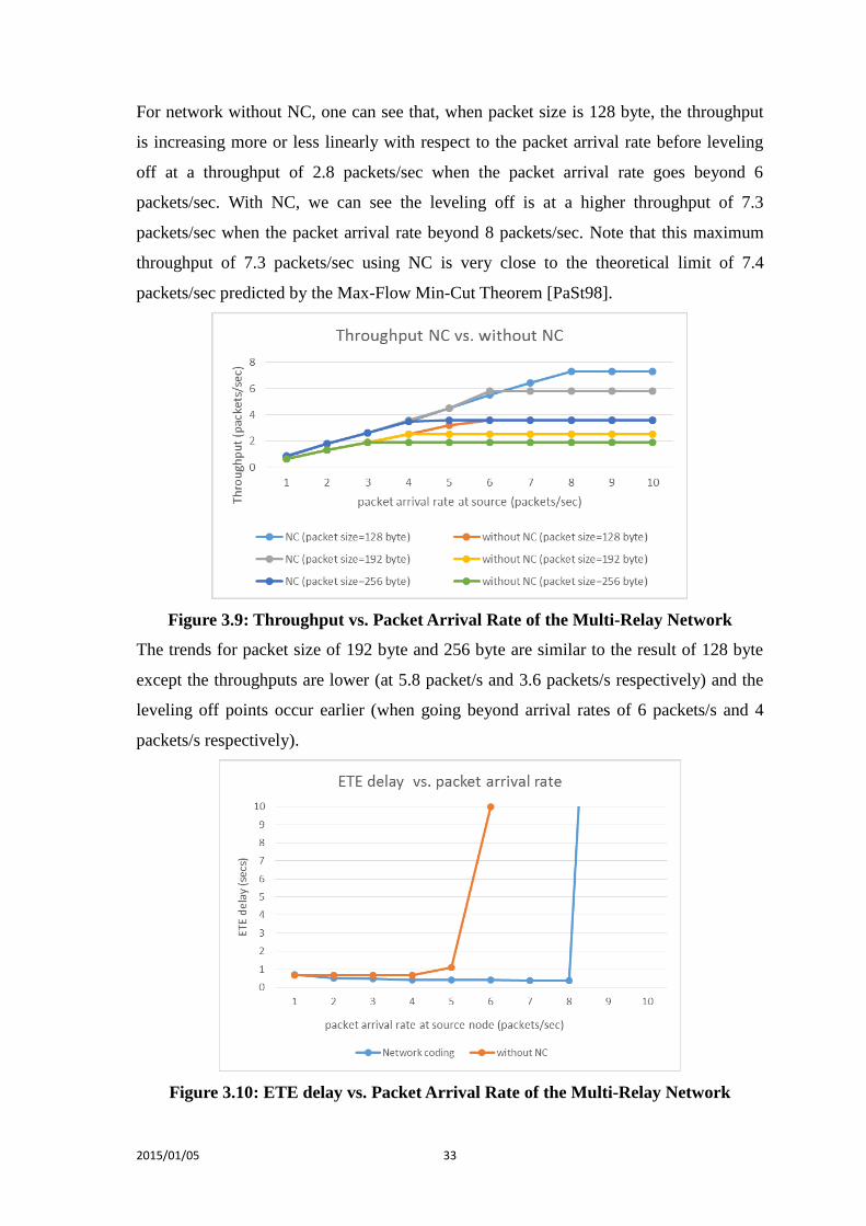
3.2.2.1 Throughput ................................................................................................... 32
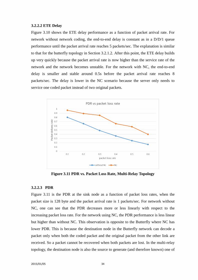
3.2.2.2 ETE Delay .................................................................................................... 34
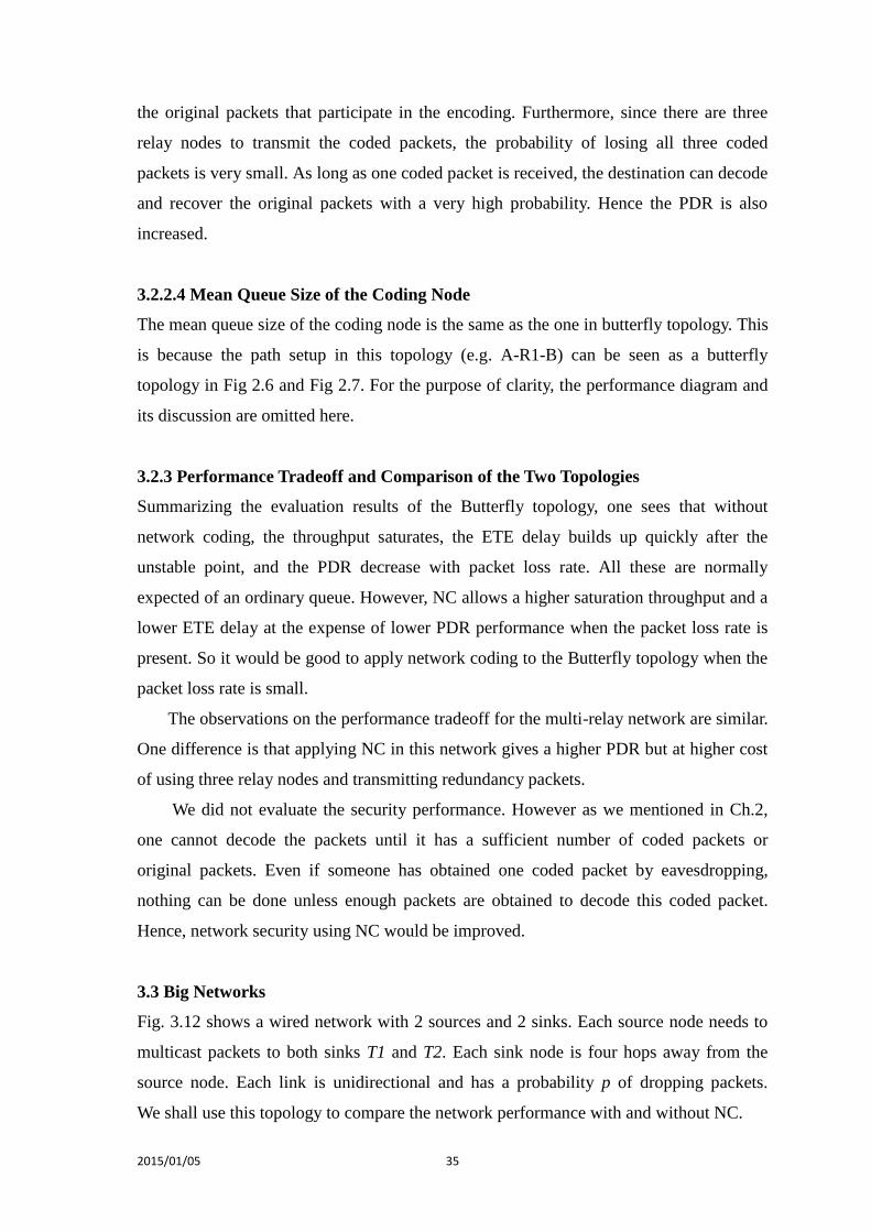
3.2.2.3 PDR .............................................................................................................. 34
3.2.2.4 Mean Queue Size of the Coding Node ........................................................ 35
3.2.3 Performance Tradeoff and Comparison of the Two Topologies ..................... 35
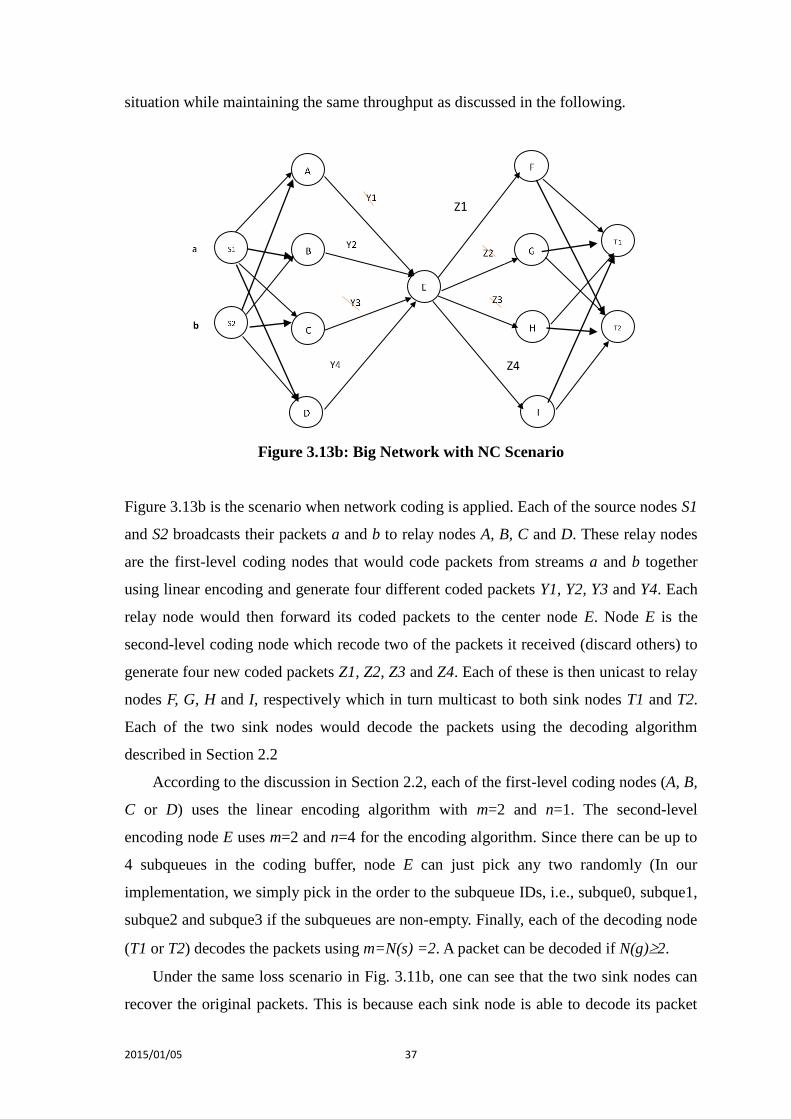
3.3 Big Network ............................................................................................................ 35
3.3.1 Performance Evaluation .................................................................................. 38
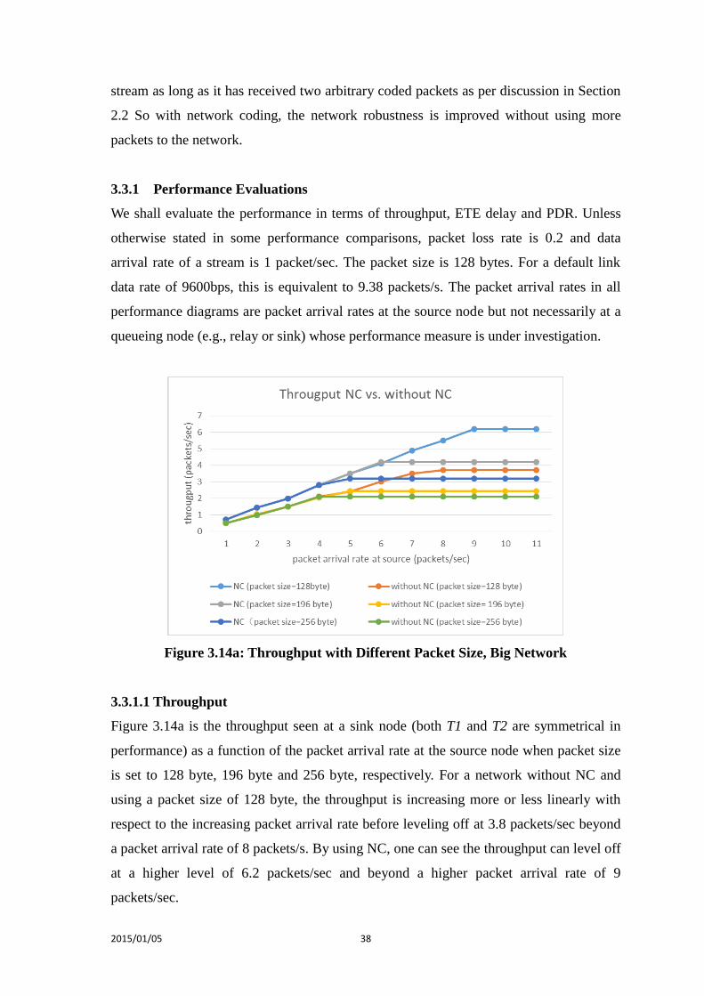
3.3.1.1 Throughput ................................................................................................... 38
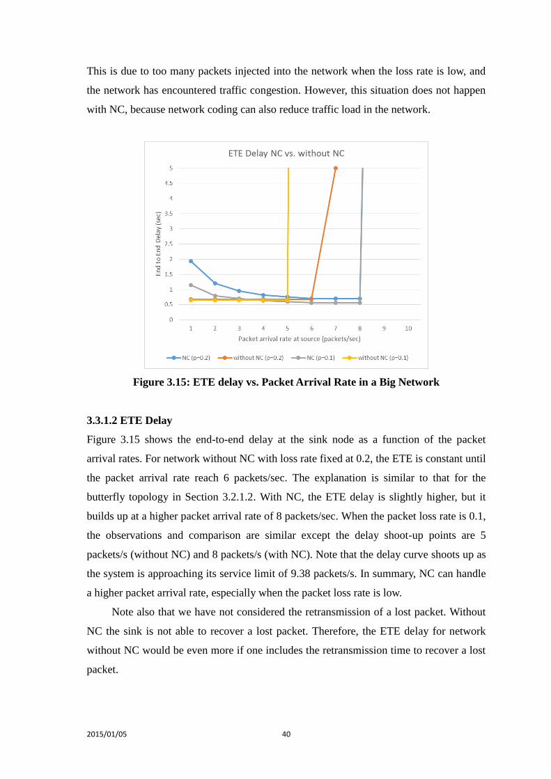
3.3.1.2 ETE Delay .................................................................................................... 40
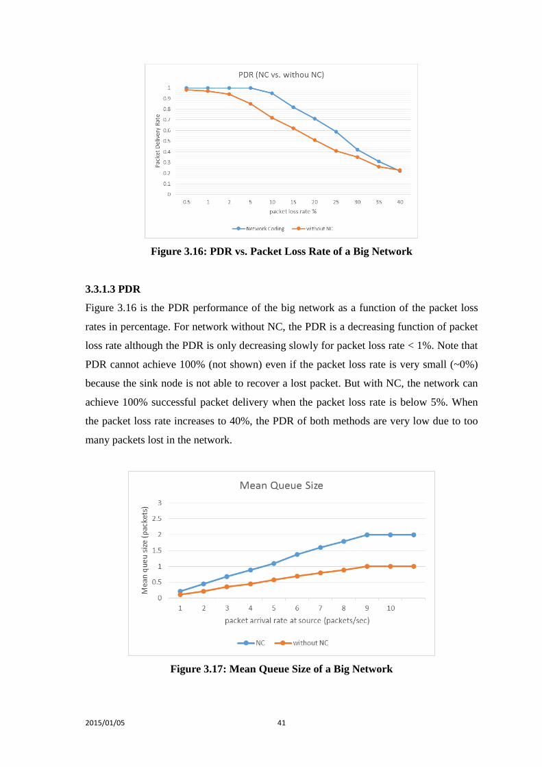
3.3.1.3 PDR .............................................................................................................. 41
3.3.1.4 Mean Queue Size ......................................................................................... 42
2015/01/05 v
3.3.2 Performance Tradeoff ..................................................................................... 42
3.4 Concluding Remarks .............................................................................................. 42
4. Three Dimensional Underwater Network ......................................................... 44
4.1 Underwater Channel Characterization for OPNET Design .................................... 44
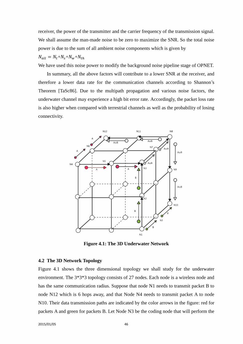
4.2 The 3D Network Layout ......................................................................................... 46
4.2.1 Network Parameters ........................................................................................ 47
4.3 Performance Evaluation .......................................................................................... 47
4.3.1 Throughput ...................................................................................................... 48
4.3.2 ETE Delay ....................................................................................................... 49
4.3.3 PDR ................................................................................................................. 50
4.3.4 Comparison with Terrestrial Network ............................................................. 50
4.4 Concluding Remarks .............................................................................................. 50
5. Design Issues and Guidelines ................................................................................. 51
5.1 Choice of Topology ................................................................................................ 51
5.2 Coding and Decoding Complexity ......................................................................... 51
5.3 Tradeoff ................................................................................................................... 52
5.4 Limitations .............................................................................................................. 52
6. Conclusions .............................................................................................................. 54
6.1 Future Work ............................................................................................................ 54
References .................................................................................................................... 56
Appendix A Examples of the Benefits of Network Coding .................................. 59
Appendix B OPNET Radio Transceiver Pipeline Stages ..................................... 63
2015/01/05 vi
List of Figures Figure 2.1 Network Layout ................................................................................ 13
Figure 2.2 Coding at A Node .............................................................................. 14
Figure 2.3 Queueing at a Coding Node .............................................................. 16
Figure 2.4 Flowchart of Coding Node ............................................................... 17
Figure 2.5 Flowchart of Decoding ..................................................................... 18
Figure 2.6 Half Duplex Wireless Operation via a Relay Node .......................... 19
Figure 2.7 Corresponding Wireless Butterfly Topology .................................... 19
Figure 2.8a Packet form a Source ........................................................................ 20
Figure 2.8b Coded Packet from a Coding Node .................................................. 20
Figure 2.9 OPNET Node Model of Coding Node .............................................. 21
Figure 2.10 OPNET Process model: NC Process Model ..................................... 22
Figure 2.11 OPNET Transceiver Pipeline Stage .................................................. 23
Figure 3.1 Butterfly Topology ............................................................................ 26
Figure 3.2 Throughput vs. Arrival Rate, Butterfly Topology ............................. 27
Figure 3.3 End to End Delay vs Arrival Rate, Butterfly Topology .................... 28
Figure 3.4 PDR vs. Packet Loss Rate, Butterfly Topology ................................ 29
Figure 3.5 Mean Queue Size vs Packet Arrival Rate, Butterfly Topology ........ 29
Figure 3.6 Mean Queue Size of Subqueue0 ....................................................... 30
Figure 3.7 95% Confidential Interval of Mean Queue Length .......................... 31
Figure 3.8 Multi-Relay Topology ....................................................................... 32
Figure 3.9 Throughput vs. Packet Arrival Rate of the Multi-Relay Network .... 33
Figure 3.10 ETE delay vs. Packet Arrival Rate of the Multi-Relay Network ...... 33
Figure 3.11 PDR vs. Packet Loss Rate, Multi-Relay Topology ........................... 34
Figure 3.12 Big Network Topology ..................................................................... 36
Figure 3.13a Big Network without NC Scenario ................................................... 36
Figure 3.13b Big Network with NC Scenario ........................................................ 37
Figure 3.14a Throughput with Different Packet Size, Big Network ..................... 38
Figure 3.14b Throughout vs. Packet Arrival Rate in a Big Network ..................... 39
Figure 3.15 ETE delay vs. Packet Arrival Rate in a Big Network ....................... 40
Figure 3.16 PDR vs. Packet Loss Rate of a Big Network.................................... 41
Figure 3.17 Mean Queue Size of a Big Network ................................................. 41
Figure 4.1 3D Underwater Network ................................................................... 46
Figure 4.2 Underwater Network Throughput ..................................................... 48
Figure 4.3 Underwater End to End Delay .......................................................... 49
Figure 4.4 PDR, Underwater Network ............................................................... 49
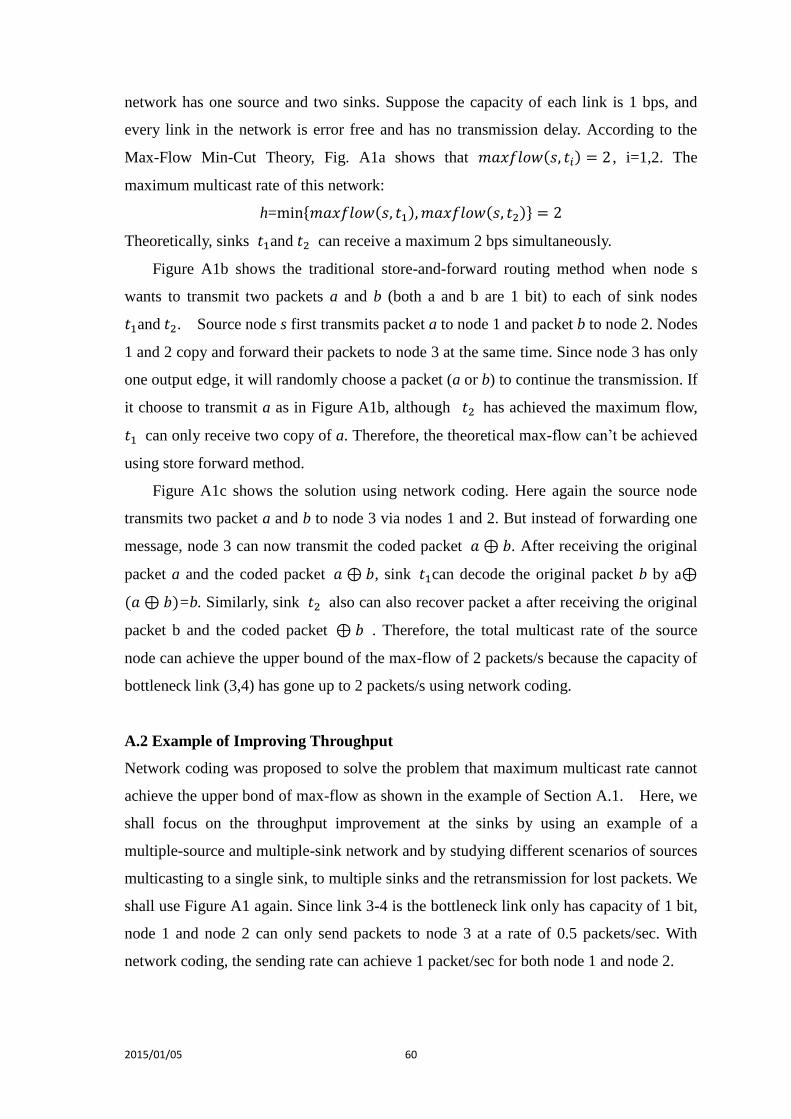
Figure A1 Example of Butterfly Network ......................................................... 59
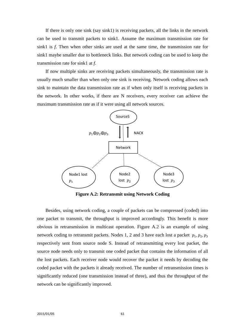
Figure A2 Retransmit using Network Coding ................................................... 61
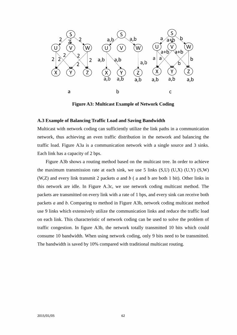
Figure A3 Multicast Example of Network Coding ............................................ 62
Figure B1 OPNET Transceiver Pipeline Stages ................................................ 63
2015/01/05 vii
List of Acronyms and Abbreviation Section of
1st Reference
ACK ACKnowledgment 1.2.3.3
CAMR Coding Aware Multipath Routing 1.2.3.2
CCACK Cumulative Coded ACKnowledgment 1.2.3.1
CLONE Coding with LOss awareNEsss 1.2.2
CSMA/CA Carrier Sense Multiple Access/Collision Avoidance 1.2.2
ECX Expected Coding Number 1.2.3.2
ETE End To End 3.2.1.2
HOL Head Of Line 2.2.1
MAC Media Access Control 1.2.2
MORE MAC-independent Opportunistic Routing & Encoding 1.2.3.1
NC Network Coding 1.2.2
OMNC Optimized Multipath Network Coding 1.2.3.1
OPNET Optimized Network Engineering Tools 1.4
RCR Adaptive Coding aware Routing 1.2.3.2
PDR Packet Delivery Ratio 3.1
PCMRDT Practical Coding based Multi-hop Reliable Data Transfer 1.2.2
ROCX Routing with Opportunistically Coded eXchanges 1.2.3.2
TCP Transmission Control Protocol 1.2.3.2
UAN Underwater Acoustic Network 1.1
UASN Underwater Acoustic Sensor Network 1.2.2
VBF Vector Based Forwarding 1.2.2
2015/01/05 viii
List of Notations and Symbols Section of
1st Reference λ packet arrival rate 3.2.1
μ service rate 3.2.1
d distance 4.1
f frequency 4.1
m the number of original packets code together 2.2
n the number of coded packets 2.2
𝑁𝑡 turbulence noise 4.1
𝑁𝑠 shipping noise 4.1
𝑁𝑤 wind driven wave noise 4.1
𝑁𝑡ℎ thermal noise 4.1
N(g) the number of packets in the same generation 2.2.2
N(s) the number of sources 2.2.2
q queue size 3.2.1.3
w wind speed 4.1
X original packet 2.2
Y coded packet 2.2
2015/01/05 1
Chapter 1
Introduction
1.1 Overview
Along with its development, network communication desires a higher quality of data
transmission. How to make a better use of the network resources and to improve the
network performance becomes an essential topic in the research of communication
networks.
In traditional operation, nodes in the network use the store-forward mechanisms,
and network transmission performance is restrained by the capacity of some bottleneck
links. According to the Maximum Flow Minimum Cut theory [PaSt98], the transmission
rate between the transmitters and receivers cannot exceed the maximum flow of the
network. So the traditional multipath routing usually cannot reach the upper bound of the
maximum flow. Comes network coding which breaks the traditional way of data
transmission. With network coding, the intermediate nodes no longer just forward
packets only. They are allowed to process the packets, and combine two or several
income packets into one or several output packets for transmission. This makes it
possible to use less network bandwidth to send the same amount of information. Finally,
the original packets can be recovered in their destinations.
Network coding technology is a breakthrough in network communication field. It
has been widely studied in recent years due to its potential benefits of improving the
throughput of the network, reducing transmission times, improving end-to-end
performance and providing a high degree of network reliability. It can also balance traffic
load, save bandwidth and improve the network security. Protocols and routing algorithms
based on network coding are applied to wired or wireless communication. With its ability
of improving network performance, it could also be applied to wireless multi-hop
networks, ad-hoc networks, wireless sensor networks and especially underwater sensor
networks.
UAN (Underwater Acoustic Network) is an application of wireless networks which
uses acoustic as the data transmission medium in underwater environment. Compare with
terrestrial radio channel, underwater channel has many natural loss factors such as ocean
noise, Doppler shift, multipath effect and transmission fading. These unique
characteristics of UAN cause long propagation delay, high bit error rate, limited
bandwidth and limited energy, and make it difficult to achieve effective data transmission
2015/01/05 2
[AkPo05]. Considering its promising abilities of error recovery and throughput
improvement, we believe network coding can be an effective way to solve the problems
to underwater networks.
1.2 Literature Review
We shall review below work related to our research topics.
1.2.1 Network Coding Algorithms
Network coding concept is first proposed by R. Ahlswede et al [AhCa00]. From the
perspective of information flow, they proved that in a multicast network with a single
source and multiple sinks, the maximum throughput of the network as determined by the
max-flow min-cut theory can be achieved by using a simple network coding; the
bandwidth can be saved also.
The basic characteristic of network coding is the optimal processing of different
transmission data. This should be directly reflected by the different design of coding
strategies, and the code structure is the primary concern. So the original research in
network coding mainly focus on the coding algorithms, the improvement of performance
brought by a coding strategy and the complexity degree of the coding algorithm. The
design of a code structure algorithm should guarantee the intended nodes can decode the
original packets after they received a certain amount of coded packets. In the meanwhile,
the coding complexity should be reduced. The coding structure algorithms studied so far
can be divided into three categories: linear coding, algebraic coding and random coding.
A linear coding construction was proposed for its simplicity and practicability
[LiYe03]. A multicast network is formulated and it is proved that the max-flow bound
can be reached through a linear coding multicast. Linear coding also includes the
polynomial time algorithm [SaEg03]. But perhaps the simplest form is the coding based
on the XOR operation. That is, just perform the Exclusive-OR operation on the bits of
two packets. There are many XOR-based protocols such as COPE [KaRa06] and ROCX
(Routing with Opportunistically Coded eXchanges) [NiSa06]. In the proposed algebraic
framework-based coding strategy [KoMe03], a polynomial algorithm was used to solve
network problems and an algebraic tool was provided to the research of network coding.
A randomized network coding for multiple source multicast networks was introduced in
[HoMe03], where the success probability of the randomized coding in networks with
unreliable and delay links was demonstrated.
2015/01/05 3
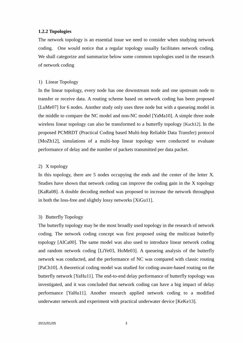
1.2.2 Topologies
The network topology is an essential issue we need to consider when studying network
coding. One would notice that a regular topology usually facilitates network coding.
We shall categorize and summarize below some common topologies used in the research
of network coding
1) Linear Topology
In the linear topology, every node has one downstream node and one upstream node to
transfer or receive data. A routing scheme based on network coding has been proposed
[LuMe07] for 6 nodes. Another study only uses three node but with a queueing model in
the middle to compare the NC model and non-NC model [YaMa10]. A simple three node
wireless linear topology can also be transformed to a butterfly topology [Ksch12]. In the
proposed PCMRDT (Practical Coding based Multi-hop Reliable Data Transfer) protocol
[MoZh12], simulations of a multi-hop linear topology were conducted to evaluate
performance of delay and the number of packets transmitted per data packet.
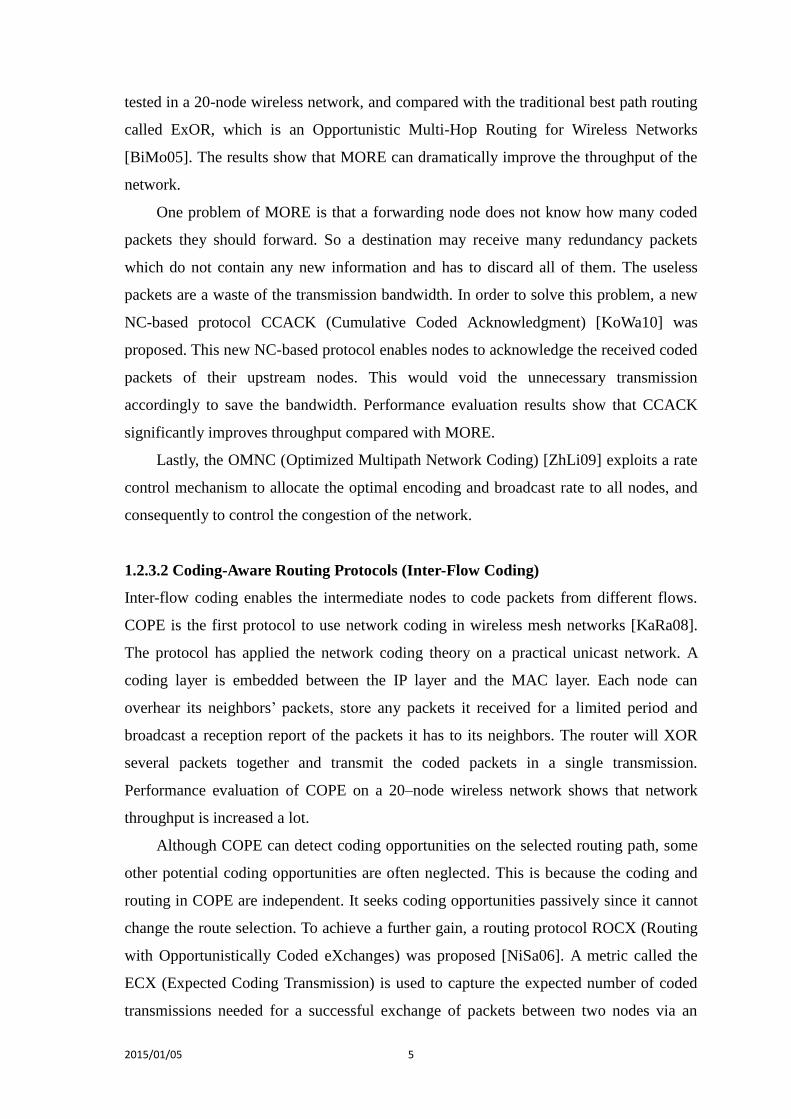
2) X topology
In this topology, there are 5 nodes occupying the ends and the center of the letter X.
Studies have shown that network coding can improve the coding gain in the X topology
[KaRa08]. A double decoding method was proposed to increase the network throughput
in both the loss-free and slightly lossy networks [XiGu11].
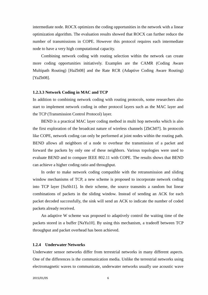
3) Butterfly Topology
The butterfly topology may be the most broadly used topology in the research of network
coding. The network coding concept was first proposed using the multicast butterfly
topology [AlCa00]. The same model was also used to introduce linear network coding
and random network coding [LiYe03, HoMe03]. A queueing analysis of the butterfly
network was conducted, and the performance of NC was compared with classic routing
[PaCh10]. A theoretical coding model was studied for coding-aware-based routing on the
butterfly network [YaHu11]. The end-to-end delay performance of butterfly topology was
investigated, and it was concluded that network coding can have a big impact of delay
performance [YaHu11]. Another research applied network coding to a modified
underwater network and experiment with practical underwater device [KeKe13].
2015/01/05 4
4) Diamond Topology
The diamond topology is usually used to emphasize the high error recovery
characteristics of random network coding. The benefit of efficient error recovery rate was
illustrated in [GuXi06], and the coding scheme was applied to underwater networks
using VBF (Vector Based Forwarding) routing. The diamond topology was also used and
implemented in a real UASN (Underwater Acoustic Sensor Network) model [MaMi13].
5) Random Topology
In addition to the regular topologies, some researchers have applied network coding to
random topologies. A suite of algorithms for network CLONE (Coding with LOss
awareNEss) operation [RaSe08] was proposed by introducing adequate redundancy in
local network coding operations. Simulation is the main tool for performance evaluation.
One research evaluated the throughput performance of coding-aware multipath routing
and single-path routing based on a 15-node random wireless topology [SeRa10]. Others
also analyzed the impact of network coding on the MAC (Medium Access Control)
protocol based on the CSMA/CA (Carrier Sense Multiple Access/Collision Avoidance)
mechanism and conducted simulations on a topology with 50 randomly-distributed nodes
[CaGo13].
1.2.3 Routing Protocols with Network Coding
Coding-based routing protocols are practical implementation of network coding.
Researchers have realized that the combination of localized NC and route selection
would further improve the performance of wireless networks [IqDa11]. Much research
has been done to combine coding and routing in both theoretical analysis and practical
system design. There are two basic categories: coding-based routing and coding-aware
routing. The difference between them is whether the coded packets come from the same
information flow.
1.2.3.1 Coding-Based Routing Protocols (Intra-Flow Coding)
Coding-based routing is also known as intra-flow network coding where routers can only
code packets from the same flow [IqDa11]. In the coding-based protocol with MORE
(MAC-independent Opportunistic Routing & Encoding) [ChJe07], the source breaks up
the file into batches of K packets. Before forwarding, the source randomly mixes the K
packets into a linear combination and broadcast the coded packets. MORE is also been
2015/01/05 5
tested in a 20-node wireless network, and compared with the traditional best path routing
called ExOR, which is an Opportunistic Multi-Hop Routing for Wireless Networks
[BiMo05]. The results show that MORE can dramatically improve the throughput of the
network.
One problem of MORE is that a forwarding node does not know how many coded
packets they should forward. So a destination may receive many redundancy packets
which do not contain any new information and has to discard all of them. The useless
packets are a waste of the transmission bandwidth. In order to solve this problem, a new
NC-based protocol CCACK (Cumulative Coded Acknowledgment) [KoWa10] was
proposed. This new NC-based protocol enables nodes to acknowledge the received coded
packets of their upstream nodes. This would void the unnecessary transmission
accordingly to save the bandwidth. Performance evaluation results show that CCACK
significantly improves throughput compared with MORE.
Lastly, the OMNC (Optimized Multipath Network Coding) [ZhLi09] exploits a rate
control mechanism to allocate the optimal encoding and broadcast rate to all nodes, and
consequently to control the congestion of the network.
1.2.3.2 Coding-Aware Routing Protocols (Inter-Flow Coding)
Inter-flow coding enables the intermediate nodes to code packets from different flows.
COPE is the first protocol to use network coding in wireless mesh networks [KaRa08].
The protocol has applied the network coding theory on a practical unicast network. A
coding layer is embedded between the IP layer and the MAC layer. Each node can
overhear its neighbors’ packets, store any packets it received for a limited period and
broadcast a reception report of the packets it has to its neighbors. The router will XOR
several packets together and transmit the coded packets in a single transmission.
Performance evaluation of COPE on a 20–node wireless network shows that network
throughput is increased a lot.
Although COPE can detect coding opportunities on the selected routing path, some
other potential coding opportunities are often neglected. This is because the coding and
routing in COPE are independent. It seeks coding opportunities passively since it cannot
change the route selection. To achieve a further gain, a routing protocol ROCX (Routing
with Opportunistically Coded eXchanges) was proposed [NiSa06]. A metric called the
ECX (Expected Coding Transmission) is used to capture the expected number of coded
transmissions needed for a successful exchange of packets between two nodes via an
2015/01/05 6
intermediate node. ROCX optimizes the coding opportunities in the network with a linear
optimization algorithm. The evaluation results showed that ROCX can further reduce the
number of transmissions in COPE. However this protocol requires each intermediate
node to have a very high computational capacity.
Combining network coding with routing selection within the network can create
more coding opportunities initiatively. Examples are the CAMR (Coding Aware
Multipath Routing) [HaZh08] and the Rate RCR (Adaptive Coding Aware Routing)
[YaZh08].
1.2.3.3 Network Coding in MAC and TCP
In addition to combining network coding with routing protocols, some researchers also
start to implement network coding in other protocol layers such as the MAC layer and
the TCP (Transmission Control Protocol) layer.
BEND is a practical MAC layer coding method in multi hop networks which is also
the first exploration of the broadcast nature of wireless channels [ZhCh07]. In protocols
like COPE, network coding can only be performed at joint nodes within the routing path.
BEND allows all neighbors of a node to overhear the transmission of a packet and
forward the packets by only one of these neighbors. Various topologies were used to
evaluate BEND and to compare IEEE 802.11 with COPE. The results shows that BEND
can achieve a higher coding ratio and throughput.
In order to make network coding compatible with the retransmission and sliding
window mechanisms of TCP, a new scheme is proposed to incorporate network coding
into TCP layer [SuSh11]. In their scheme, the source transmits a random but linear
combinations of packets in the sliding window. Instead of sending an ACK for each
packet decoded successfully, the sink will send an ACK to indicate the number of coded
packets already received.
An adaptive W scheme was proposed to adaptively control the waiting time of the
packets stored in a buffer [NaYu10]. By using this mechanism, a tradeoff between TCP
throughput and packet overhead has been achieved.
1.2.4 Underwater Networks
Underwater sensor networks differ from terrestrial networks in many different aspects.
One of the differences is the communication media. Unlike the terrestrial networks using
electromagnetic waves to communicate, underwater networks usually use acoustic wave
2015/01/05 7
to transmit data due to its low attenuation in underwater media [AyAz11]. On the other
hand, the data rates (bandwidth) of these communication channels are usually not high
and must be efficiently shared even there may not be a lot of traffic from each source.
Currently, the researches and applications on underwater network coding are still at their
infancy since the technology of network coding is not as mature as air wireless
communications. We only found a handful of related papers.
A network coding scheme based on VBF (Vector Based Forwarding) routing for
underwater sensor network has been proposed [GuXi06]. Simulations showed that
multipath forwarding with network coding scheme is more efficient for error recovery
than single-path and even multiple-path forwarding without network coding. Different
routing schemes with network coding have been compared [LuMe07] in order to provide
an underwater acoustic channel model. The numerical results show that network coding
scheme has a better performance of transmission delay in the condition of high traffic
loads. A new scheme of network coding using implicit acknowledgement is also
proposed to decrease power consumptions of the nodes [LuMe07].
Network coding has also been applied to a 2-D “cluster string topology” [ChCh10].
The results show that network coding has the advantages in high error recovery and good
energy consumption. A guideline and parameter setting in network coding is also
provided. As an extension of the work of [GuXi06], the network coding algorithm is
applied to a real underwater sensor network using both hardware and software [MaMi13].
The results indicated that network coding improved the throughput and packet delivery
rate in underwater sensor network. Network coding was also implemented in a practical
underwater device in shallow water [KeKe13] with low data rates (inter-transmission
time of 2s to 20s). The performances of a modified underwater butterfly network are
evaluated. The experiment results are provided and analyzed.
In addition to the static two-dimensional underwater networks [AkPo05],
three-dimensional networks with acoustic wireless nodes are regularly used to detect
ocean phenomena which the two dimensional network may not be able to observe
adequately. In three-dimensional underwater networks, sensor nodes float at different
depth levels in order to observe a given phenomenon [AkPo05]. Moreover, the
underwater channel is quite different from the terrestrial channel. A survey was
conducted on the existing network technology and its applicability to underwater
acoustic channels [SoSt00]. A channel model is described in order to obtain a deeper
understanding of the energy consumption in underwater acoustic networks [SeDa11].
2015/01/05 8
A combination of network coding and interference avoidance technique in
underwater environment was investigated [PaHe12]. Performances have been evaluated
and compared with CDMA/CA mechanism. The results shows NC is more efficiency and
consumed less energy.
In the work reviewed above, usually only one or two aspects of network
performances are studied. There was no comprehensive evaluation of network coding
and the discussion of their tradeoff.
.
1.2.5 Benefits of Network Coding
We can summarize below some of the commonly claimed benefits of network coding in
the papers we review. Appendix A also reviews some papers that have provided
arguments/proofs/examples to these different claims.
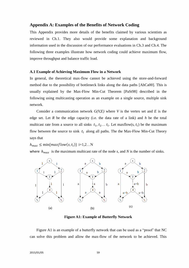
1) Achieving maximum flow:
It is known that the theoretically maximum flow of a communication network usually
cannot be achieved due to the existence of bottleneck links in the network. With network
coding, the traffic flow going through the bottleneck link can be increased without
having to increase the bandwidth (data flow rate) of the physical link. Hence, the
maximum flow of the network can be achieved. An example of the butterfly network is
shown in Appendix A1.
2) Improving throughput:
The importance of this benefit is fundamental to network coding. Using network coding,
packets can be coded in one packet for transmission and the throughput is improved
accordingly. Note that throughput is not only increased as a consequence of (1); it can
also be increased in other scenario due to network coding. For example, the original
packets can be recovered even a small number of packets are missing. Another example
in Section A2 (in Appendix A) is also provided to illustrate how improved throughput can
be achieved.
3) Balancing traffic flow and saving bandwidth:
Multicasting with network coding can sufficiently utilize the link paths in a
communication network, thus achieving an even traffic distribution in the network and
balancing the traffic load. An example is provided in Appendix A3.
4) Improving reliability
Higher reliability is the most compelling benefit of network coding especially in mobile
and/or lossy networks. Using network coding, several original packets that are linearly
2015/01/05 9
independent of each other can be coded together to form a group of new coded packets
[FrBo05]. The receiver is able to decode the original packets so long as a sufficient
number of encoded packets are received [FrBo05]. The loss of a small number of packets
does not require retransmissions. The performance of reliability gain has been evaluated
in [GhTo08]. The results shows the network coding method can reduce the times of
packet retransmission when compared to other method.
5) Enhancing security.
Another network performance would be improve by network coding is security. The
coding characteristic enhances the difficulty of cracking information from the network.
Since a node can decode the packets only if it received a sufficient number of coded
packets, an eavesdropper is not able to obtain the useful information even through it can
overhear one or several coded packets. A wiretap model using linear network coding was
proposed [CaYe10] where wire tappers cannot get the transmitted information even if
they are allowed to access the transmission channels.
1.3 Motivation and Objectives
Since Ahlswede et al. proposed the concept of network coding in year 2000, it has been
studied by many researchers in different aspects. From our literature survey, we noticed
that the performance of network coding can vary with different network topologies.
Choosing a suitable topology and appropriate coding nodes can make a better use of
network coding. Moreover, most of the papers only evaluate only one or two aspects of
the network performance. It would be desirable to have a comprehensive evaluation of
the networks on every mainly promised benefits of network coding, and to see if these
benefits can be all achieved in the same topology and conditions. If not, what tradeoffs
are in implementing the network coding to communication networks
Our literature review also show that the basic design goals of underwater networks
are maximizing throughput among nodes, saving bandwidth, decreasing energy
consumption and improving network reliability. Since these appear to be the advantages
of network coding also, we would like to apply network to underwater networks to see if
the performance of underwater networks can be improved.
The ocean is a complex and volatile environment where the signal can attenuate due
to energy absorption and diffusion loss during its transmission. Therefore, the channel
model is quite different from terrestrial channel models. We would like to establish an
underwater channel model in OPNET modeler for our simulation and future use.
2015/01/05 10
As a general objective of this thesis in view of the above discussion, we would like
to verify the promised benefits of network coding. Specifically, we would like
1) to have a more systematic and comprehensive evaluation of network coding on
some chosen topologies.
2) to compare data network communication with and without network coding in terms
of their performances and study the tradeoffs in these performances.
3) to evaluate the performance of a wireless underwater acoustic network using
network coding to see if the same benefits can be achieved.
1.4 Methodologies and Approaches
In order to achieve our objectives, we need to first understand the operation details of
network coding so that we can incorporate them into our network queueing model and
evaluate the performance properly. Through the literature review, we hope to obtain the
knowledge and operation details related to different areas including the coding
algorithms, the routing protocols with network coding, and the application of network
coding to wireless sensor network, multi-hop network and underwater acoustic networks.
As a starting point, we shall use stationary topologies in our study of network coding
because we can decide by inspection which intermediate nodes in the network should
perform the coding operation. We shall consider some regular topologies in this thesis
and observe their network performances.
Since there can be many possible topologies, we would be selective to pick a few
popular ones in the literature. We start with the butterfly topology and the multi-relay
topology which are small networks of regular topologies, We have not chosen the single
node nor the three-node linear network used by many researchers because they are a
subset of the two chosen candidates that have more features for us to study and to
compare with networks without coding in order to understand the tradeoffs. We shall
study the queueing behavior of a coding node and the network performance such as
network throughout and end-to-end delay. Then we choose some big regular topologies
in order to see and understand how network performance would change when using
different topologies and/or bigger networks.
The small and big networks we shall study all have two-dimensional topologies
that can find applications in land-based networks. We shall also extend our study to a
three-dimensional network by studying an underwater acoustic network. Here, we have
the challenge to understand first the underwater physical environment for acoustic
2015/01/05 11
propagation and therefore the impact to data communication. This would also allow us to
identify the proper channel model which we shall incorporate into our underwater
topology for the study and analysis of network coding.
Since a queuing analysis involves much time in mathematics for the time limit of
this study, we have resorted to simulation. Of all the simulation languages available in
the research world, I have chosen OPNET (Optimized Network Engineering Tools)
[OPNE14] to be our simulation modeler because that its hierarchical modeling
methodology makes it simple to use and our research group already has a lot of expertise
about exploiting OPNET.
OPNET has a sophisticated workstation-based environment for the modeling and
simulation of communication systems, protocols and networks in order to verify the
detailed operations of some protocol and to analyze their performance. On the other hand,
it is relatively easy to use once its design concepts are understood. OPNET consists of
four major components: Project Editor, Node Editor, Process Editor and Packet Editor
[OPNE14]. Project Editor is used to build the topology of a network and provide the
basic analysis capabilities and simulation. With the Node Editor, we can construct a node
with different objects and define various interfaces. The Process Editor consists of
several states connected with transition conditions; the behavior of the process is
specified using C/C++ language. The Packet Editor is used to define the internal structure
of a packet which can have several different fields and format. The debugging tool is
another very useful feature of OPNET we shall use to do debugging of our simulation
codes as well as establishing and verifying the underwater channel mentioned above.
1.5 Contributions
The main contributions of this thesis are:
1. The queueing performance evaluation of coding nodes.
2. The network performance evaluation of a small butterfly network, a multi-relay
network and a bigger network when using network coding, as well as the tradeoffs in
performance based on these studies.
3. The application of network coding to an underwater acoustic network and its
performance evaluation.
4. The OPNET modeling of an underwater channel based on existing mathematical
models so that the network performances of an underwater network can be evaluated.
2015/01/05 12
1.6 Thesis Organization
The remainder of this thesis is organized as follows. Chapter 2 gives the general network
layout under study, and describes the network operation and the assumptions used
throughout the thesis. It also describes the coding node functions, and the simulation
models used in our performance evaluations. Chapter 3 evaluates the network
performance and queueing behavior of various small and big networks in order to
analyze and verify the benefits of throughout, delay and reliability. Chapter 4 sets up the
mathematical models for the underwater channel so that Opnet simulation and
performance evaluation can be carried out for an underwater acoustic network using
network coding. Chapter 5 discusses the design issues and guidelines based on the
experience from this research. Finally, conclusion and future works are provided in
Chapter 6. The appendices contain examples of the network coding benefits and OPNET
pipeline stages.
2015/01/05 13
Chapter 2
Network Operation, Models and Assumptions
In this chapter, we shall provide the operation details of network coding at a node and
along the data path in a network. Then we implement them in the OPNET node models
and process models that are used in our simulations throughout the paper. Any general
assumptions used in our performance evaluation and analysis are provided at the end.
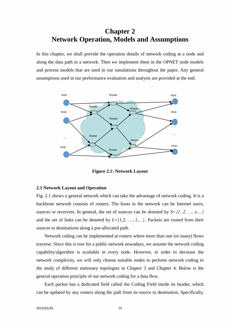
Figure 2.1: Network Layout
2.1 Network Layout and Operation
Fig. 2.1 shows a general network which can take the advantage of network coding. It is a
backbone network consists of routers. The hosts in the network can be Internet users,
sources or receivers. In general, the set of sources can be denoted by S={1, 2, …, s,…}
and the set of links can be denoted by L={1,2, …, l,…}. Packets are routed from their
sources to destinations along a pre-allocated path.
Network coding can be implemented at routers where more than one (or many) flows
traverse. Since this is true for a public network nowadays, we assume the network coding
capability/algorithm is available in every node. However, in order to decrease the
network complexity, we will only choose suitable nodes to perform network coding in
the study of different stationary topologies in Chapter 3 and Chapter 4. Below is the
general operation principle of our network coding for a data flow.
Each packet has a dedicated field called the Coding Field inside its header, which
can be updated by any routers along the path from its source to destination. Specifically,
Router
Router
Router
Router
Router
Router
Router
Router
Host
Host
Host
Host
Host
Host
…
… …
2015/01/05 14
each router updates the coding vectors in the Coding Field of a packet header. At the
destination, the receiver can use the coding vectors to decode the packets. The
computation of coding and decoding using coding vectors will be described in Section
2.2.
2.2 Network Coding at a Node
Although each node has the capability to perform network coding, it does not need to if
there is no such requirement. In fact, study shows that by choosing proper nodes in a
network to perform network coding, network computational complexity and decoding
processes can be reduced [ClTo11].
A node is called a coding node if chosen to perform network coding. When chosen, it
operates on multiple packets from different information flows passing through. It outputs
packets that are combinations of the input packets after some computations as detailed
below.
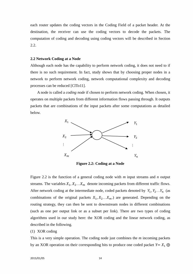
Figure 2.2: Coding at a Node
Figure 2.2 is the function of a general coding node with m input streams and n output
streams. The variables 𝑋1, 𝑋2…𝑋𝑚 denote incoming packets from different traffic flows.
After network coding at the intermediate node, coded packets denoted by 𝑌1, 𝑌2…𝑌𝑛 (as
combinations of the original packets 𝑋1, 𝑋2…𝑋𝑚.) are generated. Depending on the
routing strategy, they can then be sent to downstream nodes in different combinations
(such as one per output link or as a subset per link). There are two types of coding
algorithms used in our study here: the XOR coding and the linear network coding, as
described in the following.
(1) XOR coding
This is a very simple operation. The coding node just combines the m incoming packets
by an XOR operation on their corresponding bits to produce one coded packet Y= 𝑋1 ⊕
𝑋1
𝑋2
𝑋𝑚
….
𝑌1
𝑌2
𝑌𝑛
….
2015/01/05 15
𝑋2 ⊕ … ⊕ 𝑋𝑚. Decoding is simply done by using X𝑗 = Y ⊕ 𝑋1 … ⊕ 𝑋𝑗−1 ⊕ 𝑋𝑗+1 ⊕
… ⊕ 𝑋𝑚. In other words, as long as a receiver node has received the coded packet Y
and any m-1 of the original packets, it can always decode the remaining original packet.
(2) Linear network coding
Here, we have 𝑌𝑖 = ∑ (𝑔𝑖𝑗𝑋𝑗)𝑚𝑗=1 where indicates summation under the GF(2𝑆)
operation, and gij is the coding coefficient associated with packet Xj. In matrix form, we
have
[
𝑔11 ⋯ 𝑔1𝑚
⋮ ⋱ ⋮𝑔𝑛1 ⋯ 𝑔𝑛1
] [𝑋1
⋮𝑋𝑚
] = [𝑌1
⋮𝑌𝑛
]
On passing, one would observe that the XOR coding in (1) is just a special case of the
linear network coding using GF(21) where S=1.
Encoding can also be performed recursively on coded packets [FrBo06]. If a node
has received a couple of coded packets (𝑔1, 𝑌1), (𝑔2, 𝑌2) … . . (𝑔𝑛, 𝑌𝑘) , where 𝑔𝑖
=(𝑔𝑖1, 𝑔𝑖2 … 𝑔𝑖𝑚) is the coding vector of 𝑌𝑖, this node can also linearly combine these
packets with another set of coefficient 𝑓𝑖1, 𝑓𝑖2…𝑓𝑖𝑘and output new coded packets:
𝑍𝑖 = ∑(𝑓𝑖𝑗𝑌𝑗)
𝑘
𝑗=1
The new coding vector is updated to:
𝑔𝑖′ = ∑(𝑓𝑖𝑗𝑔𝑖)
𝑘
𝑗=1
In order to decode an encoded packet at a receiver, the coefficients 𝑔𝑖1, 𝑔𝑖2…𝑔𝑖𝑚
should be chosen independently and randomly from a finite Galois Field GF(2𝑆)
with 2𝑆elements [FrBo06], where S is the degree of the polynomial. The coding vector
𝑔𝑖 = (𝑔𝑖1, 𝑔𝑖2 … 𝑔𝑖𝑚) has to travel with the coded packet Yi. This vector is placed in the
Coding field inside the packet header mentioned earlier.
Assume a receiver has received all n coded packets (𝑔1, 𝑌1), (𝑔2, 𝑌2) … . . (𝑔𝑛, 𝑌𝑛) in
the set. In order to recover the original packets 𝑋1, 𝑋2…𝑋𝑚, we need to solve a linear
system of m unknowns and n equations [FrBo06]. In matrix form, we have
[𝑋1
⋮𝑋𝑚
] = [
𝑔11 ⋯ 𝑔1𝑚
⋮ ⋱ ⋮𝑔𝑛1 ⋯ 𝑔𝑛1
]
−1
[𝑌1
⋮𝑌𝑚
]
2015/01/05 16
where [M]−1 indicate the inverse of the matrix M. In practice, one can use the Gaussian
Elimination Method [FrBo06, KeAt89]. If 𝑛 ≥ 𝑚, the receiver can recover the original
packets successfully by using the reverse of the coding vector matrix. In other words, so
long as the receiver can receive a least m coded packets along with their coding vectors,
the original packets can be recovered.
If n<m, the receiver cannot decode the original packets. This suggests that one must
produce as many coded packets as the number of original packets so that the receiver can
receive no less than m coded packets.
2.2.1 Encoding Implementation
For normal operation without network coding, packets of different lengths can arrive at a
single buffer and served in a FIFO (First In First Out) discipline. With network coding, a
packet may have to wait for another packet to carry out the coding operation. The data
portion of each packet must have the same length (number of bits) so that the coding
computation in bits can be carried out.
Figure 2.3: Queueing at A Coding Node
Fig. 2.3 shows the scenario where a node wants to perform network coding on data
traffic streams from m different incoming physical links. The coding node can be
considered as a single server queue with m infinite buffers, each storing packets from
different sources (streams). The server takes one HOL (Head Of Line) packet from each
queue and codes them into n packets. After delivering them to the outgoing links
(according to some specified routing algorithm), the server would remove the m old
packets from their queues and repeat the same operation for the next m HOL packets.
Figure 2.4 below is the flow chart summarizing the coding operation.
Buffer 0
Buffer m
Coding
.... ....
....
2015/01/05 17
Figure 2.4: Flowchart of a Coding Node
Note that there must be a packet present in each queue (called the coding condition).
Otherwise, packets in other queues to wait for an arrival to the empty queues. All coded
packets generated from the same original packets are called “packets of the same
generation”. We also note on passing that in general, one does not require the packet
streams to come from different physical links. They can just be logical flows within the
same physical link. So the buffers in Fig. 2.3 can be used for packets of the same logical
link.
2.2.2 Decoding
In order to illustrate the decoding process explicitly, here we define N(g) as the number
of coded packets from the same generation it received, and N(s) is the number of original
packets m used in the encoding process. According to Section 2.2, one must have 𝑛 ≥ 𝑚
to recover the original packets. So whenever N(g)N(s), we know that decoding can take
place. To allow decoding, the receiver may want to have allocate at least m buffer space.
Insert it to the packet buffer
Incoming packet
Meet coding
condition?
Y
Y
Code packets, remove
HOL of each buffer, send
coded packets
N
N Wait for other
packets from
different
flowsWait for
other packets
from different
flows
2015/01/05 18
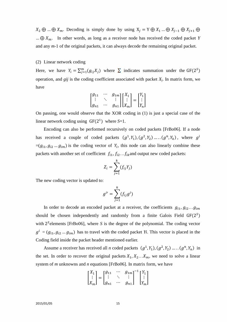
Figure 2.5: Flowchart of Decoding
Figure 2.5 is the flowchart of decoding. Note that an innovative packet is a packet useful
for decoding to recover an original packet X. A packet is non-innovative if it is not
needed any more, either because the receiver has enough coded packets from the same
generation, or the original packet has been recovered. When a coded packet arrives at the
receiver, the decoder will first check its generation number in the packet header, and
determine if it is “non-innovative”. If so, the receiver will discard this coded packet. If
the number of packets N(g) from the same generation is no less than the number of
sources N(s) (i.e. the mn case in Section 2.2), the receiver can decode all packets. In
some scenarios such as packet loss, there will not be enough packets to decode and
recover the original packets, and the receiver will discard all packets at this generation.
2.3 Topologies for Network Coding
One would notice that the operation described so far requires at least two traffic streams
to be present for network coding, and these coded streams must also be present at the
N(g)>=N(s)? Discard all coded
packets in current
generation
N
Insert it to the coded-packet
buffer
Receiving a coded packet
Is it an innovative
packet?
Y
Decode packets, extract
coded packets from
coded-packet buffer
N
Discard packet
Y
2015/01/05 19
destination for decoding. This suggests that networks with symmetric topologies would
be good candidates. Although this may not be readily present in real-life physical
networks, we nevertheless adopt the symmetric networks (such as those to be shown in
Chapters 3 and 4) as the starting point of our investigation. There are several reasons for
our choice. First, many existing works have already taken this assumption, and we can
make comparisons with their results if needed. Secondly, one can argue the coding can be
done on symmetric logical topologies even the underlying physical topologies may not
be symmetric. Routing is one resort to help to achieve the logical topologies seen in the
upper layer. Finally, some of the network operations give rise to a symmetric network
topology naturally such as the Butterfly topology depicted in Figure 3.1 of Section 3.2
later that can be used in wired network. In a wireless network, it is quite easy to
encounter topologies with the butterfly network characteristics. This is usually referred to
as the “wireless butterfly topology” [Ksch12] as described below.
Figure 2.6: Half Duplex Wireless Operation via a Relay Node [Ksch12]
Figure 2.7: Corresponding Wireless Butterfly Topology
s
r
t a b
a⊕b a⊕b
s′
t′
t
Transmitter Transmitter
Receiver Receiver
r
r′
Transmitter
Receiver
r
Transmitter
Transmitter
Transmitter
Transmitter
2015/01/05 20
Figure 2.6 is a simple three node wireless network. It depicts two wireless stations s
and t that are too far away to have direct communication. Therefore, they must
communicate through a broadcast relay node r. Suppose all three nodes are half-duplex
so that each node cannot transmit and receive packets at the same time. Then node r can
be used as a coding node if nodes s and t can synchronize their transmissions to node r.
As shown in Fig. 2.7, s and s’ represent the transmitter and receiver of node s
respectively, and likewise the notations for the other two nodes. After receiving packets
sent synchronously from both stations s and t, the relay node r is able to code the packets
and broadcast the coded packets to s and t. The resulting communication topology
resembles a butterfly.
2.4 OPNET Models
As stated in the Methodology section in Chapter 1, we are going to use OPNET for our
simulation. We present here the node, the process and the packet models used in our
OPNET simulation. They will also provide more information on the operation of our
network using network coding.
2.4.1 Packets for Network Coding
An OPNET packet in general contains several information storage areas. The most
frequently used area is the first area (called packet header) consisting of a list of fields for
user-defined information [OPNET14]. We shall customize the packet as follows:
Figure 2.8a: Packet from a Source
Figure 2.8b: Coded Packet From a Coding Node
DataField1+DataField2 Packet Header
headerPacket
headerPacket
header
Generation
Generation
Generation
Generation
Destination1
11Destinatio
n
1Destination
1Destination
1
Coding field
Coding field
Coding field
Coding field
Destination2
Destination 2
Packet Header Data Field
2015/01/05 21
Figure 2.8a is the format of a packet generated at a source node. There is only one
destination address in the packet header. Figure 2.8b illustrates the format of coded
packets from a coding node. The data field storage the data information of the coded
packet. “DataField1+DataField2” shown in the figure shows that this packet has data from
the combination of the data field of two original packets. The packet header now consists
of several fields. The Generation field records the generation number of the coded
packets so that the destination node can recognize and use the packets from the same
generation to decode the original packets. The Destination field stores the destinations
(e.g. a physical address) of the original packets (two in this case). The Coding field stores
the coding information. In XOR coding, the coding field is either an integer 0 or 1 to
distinguish whether the packet is coded or not. In linear coding, the coding field is used
to store the coding vector. The number of components in the vector also indicate the
value of m which is the number of original packets used in the encoding. Obviously, the
length of a coded packet can be different depending on how many destinations it has as
well as the size m of the coding vector.
Figure 2.9: OPNET Node Model of Coding Node
2.4.2 Node Model and Process Model
Figure 2.9 is the OPNET node model of a coding node taking traffic from two data
streams (which is the common scenario in our investigation). There are 4 objects in this
node model. Two point-to-point receivers ‘rcv” are used to receive the packets from
upstream nodes. The “nc-proc” is the coding process to handle the incoming packets and
to perform coding operation. The transmitter “xmt” is an internal point-to-point
transmitter for the transmission of packets to the next node through the network link.
2015/01/05 22
Figure 2.10: OPNET Process Model: NC Process Model
Figure 2.10 is the OPNET process model for a NC node. As shown in the figure, the
process is in the “arrival” state whenever a packet arrives. Each packet will be inserted to
corresponding subqueues according to its traffic stream. If the server is not busy and all
subqueues have a packet, it enters the “svc_start” state where the coding operation as
described in Fig. 2.4 will take place. Then it enters the “idle” state to wait for the service
of the coded packet to complete (this is what we usually call the transmission time of the
packet). At the end of its transmission, the “svc_compl” event will be triggered by a self
interrupt, and the process goes to svc_compl state where the packet is removed from the
node buffer. After this, the process will enter the idle state to wait for another packet
arrival if the subqueue has become empty, or it enters the “svc_start” state again to serve
(perform network coding) on another group of packets if they are present in all
subqueues. Note that the “idle” state allows a packet to wait for different events as noted
while the init state is a trivial state to initialize the process.
Except for the coding node model and the NC process model, we also need to create
some other node models and process models to complete the network simulation. They
are:
a. Source node: It consists of a source generator, a source process model and one or
more point to point transmitters.
b. Sink node: It consists of a decoding process, a sink process and some point to point
receivers. The decode process is the place where the decoding procedures is
executed as described in Section 2.2
2015/01/05 23
In addition to these node models and process models, we also need to create the link
model to build the whole OPNET project.
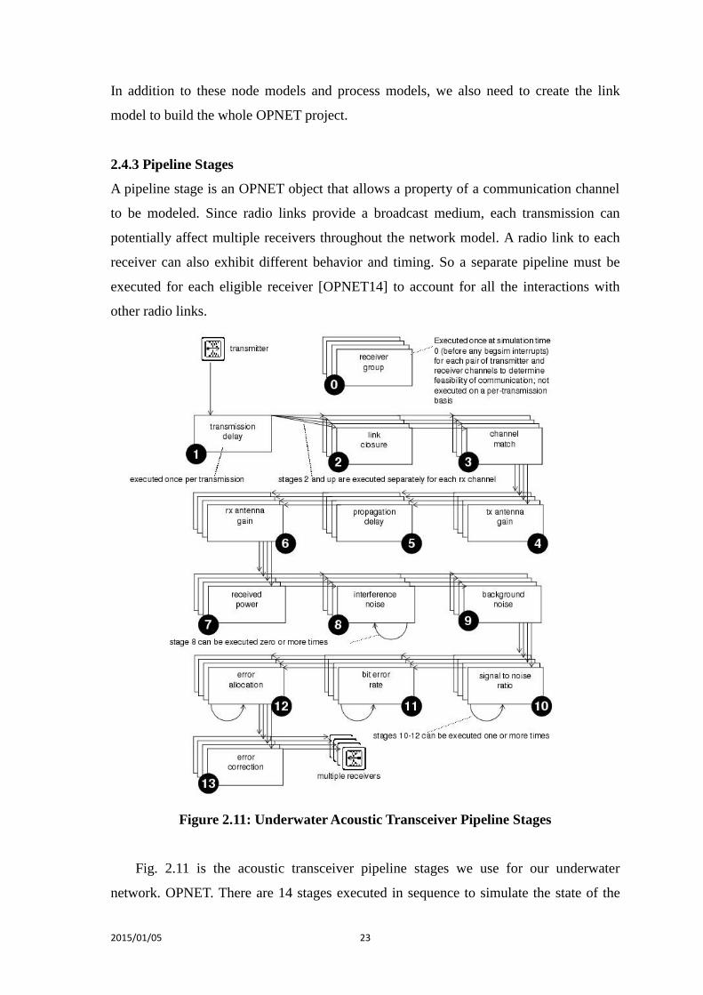
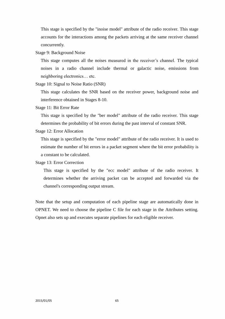
2.4.3 Pipeline Stages
A pipeline stage is an OPNET object that allows a property of a communication channel
to be modeled. Since radio links provide a broadcast medium, each transmission can
potentially affect multiple receivers throughout the network model. A radio link to each
receiver can also exhibit different behavior and timing. So a separate pipeline must be
executed for each eligible receiver [OPNET14] to account for all the interactions with
other radio links.
Figure 2.11: Underwater Acoustic Transceiver Pipeline Stages
Fig. 2.11 is the acoustic transceiver pipeline stages we use for our underwater
network. OPNET. There are 14 stages executed in sequence to simulate the state of the
2015/01/05 24
transmission channel for each packet transmission. These stages are copied directly from
the radio transceiver pipeline stage from [OPNET14] except that we have to modify the
equations and parameter values used for the wireless air channel in order to characterize
the underwater channels that we need in Ch.4. In order to match the unique underwater
features, we need to revise the propagation delay stage, the receiver power stage and the
background noise stage. The mathematical details of these customized stages will be
discussed in Section 4.2, and the detail description of each stage can be found in
Appendix B using the original wireless air channel as an example.
2.5 Assumptions
Unless otherwise stated, the following assumptions pertain to the remainder of this thesis.
(1) Buffer size is infinite. This is because memory is very cheap nowadays and one can
provide a node with a buffer large enough to have negligible loss.
(2) The networks have symmetric topologies. This is because regular network topologies
can facilitate the network coding operation, and can be constructed logically as
discussed in Section 2.3.
(3) Packet inter-arrival time is constant. This is because we want to make sure that when
a packet arrives at coding node, there is a very large probability to find a packet
present in the buffer from the other source for network coding together.
4) We do not consider higher layers in our simulations. For example, routing is
assumed done so that data flows can follow a pre-assigned path to make up a regular
topology.
5) Network coding capability is available in every node as discussed earlier.
6) The size of the data portion of each packet is the same to allow coding computation.
7) The effect of packet overhead is not considered in this thesis. This is because the
overhead arising from fixed routing and coding nodes is very small.
2015/01/05 25
Chapter 3
Two Dimensional Networks
As we mentioned in Chapter 2, network coding may improve the network throughput,
decrease end-to-end delay and enhance the reliability of the network. In this chapter, we
shall investigate these benefits of network coding in small networks as well as big
networks. We shall also compare the scenarios with and without network coding. Before
we do that, we shall first provide information on our simulation and performance
evaluations.
3.1 The OPENT Simulation and Performance Evaluation
The following performance measures are used in our simulations and defined as follows:
(1) Throughput: this is the average number of packets per unit time. In our simulation,
we divide the accumulated number of packets successfully received at a sink node by
the total duration of time within which the packets are collected
(2) End to end delay: this is the time spent by a packet from its arrival at a source node
until its reception at the destination. This duration can have different components
including the propagation delay, the queueing delay, the transmission delay and the
processing delay. This is measured in OPNET from the time a packet is generated in
the source node until the time it is successfully received by the sink node.
(3) Mean queue size: this is the average number of packets in the buffer of a coding node
seen by a departing packet after the system achieves steady state.
(4) Packet Delivery Ratio (PDR): this is defined to be the percentage of packets from the
source that are successfully received at the intended receiver.
The OPENT node model and process model have been illustrated in Section 2.4. All
simulations are run in a computer platform using an Intel Core2 T6600 processor running
at 2.20 GHz with 4 GB of memory. The operating system is Windows 7. We have
determined that a typical simulation would need to collect about 36000 packets to reach
the steady state of a statistics (e.g., the mean queue length). A typical simulation would
take about 8s to complete. We also run each simulation 4 times, each with a different
seed, in order to obtain a 95% confidential interval. An example is shown in Section
2015/01/05 26
3.2.1.3. Since the intervals are generally small, they are omitted for other curves in this
thesis for clarity reason.
3.2 Small Networks
The Butterfly and the Multi-Relay are the two small topologies for which we study and
evaluate the performance. Due to the symmetry in these networks, there are two sources
to be considered. We make the packet arrival rates of two sources the same. The data rate
of each link is 9600 bits/sec. When mentioned in the text or in a diagram, subqueue 0 is
understood to be the buffer for packets coming from source A, and subqueue 1 is the
buffer for packets coming from source B.
Figure 3.1: Butterfly Topology
3.2.1 Butterfly Topology
Figure 3.1 is a modified butterfly topology consisting of six nodes and 7 unidirectional
links. This is a two-source two-sink network. Node A and node B are the source nodes.
Each node needs to multicast its packets to two destination nodes, node E and node F.
Link C-D becomes the “bottleneck link” because traffic congestion may arise in this link
when shared by the communication paths of both node pairs (A,F) and (B,E). We shall
use the intermediate node C as a coding node. This node contains two data buffers to
store packets coming from node A and node B. It combines the packets form each buffer
using XOR coding (as discussed in Section 2.2) before sending the coded packet to node
D. The simple purpose of this intermediate node is to forward the coded packets to each
destination node E and F.
B A
C
D
E F
2015/01/05 27
Unless otherwise stated in some performance comparison, packet loss rate is zero,
data arrival rate of a stream is 1 packet/sec. The service capacity of the intermedia node
is 9600 bps. For a packet size of 128 bytes, a link data rate of 9600bps is equivalent to
9.38 packets/s =9600bps/(128*8bits/packet). Note that the packet arrival rates in all
performance diagrams are the arrival rates at the source node but not necessarily at the
queueing node (e.g. sink or coding node) whose performance measure is under
investigation.
Figure 3.2: Throughput vs. Arrival Rate, Butterfly Topology
3.2.1.1 Throughput
Fig. 3.2 is the throughput at the sink node as a function of the arrival rate at the source
node when the packet size is fixed at 128 bytes, 192 byte and 256 byte respectively. For
network without NC, one can see that, when the packet size is 128 byte, the throughput is
increasing more or less linearly with respect to the increasing packet arrival rate before
leveling off at 4.5 packets/s beyond the packet arrival rate of 5 packets/sec. Using NC,
one can see the leveling off at a higher throughput of 8.7 packets/s and beyond a larger
packet arrival rate of 9 packets/sec.
The trends for packet size of 192 byte and 256 byte are similar to the result of 128
byte except the throughput levels are lower (at 5.8 packet/s and 4.5 packets/s respectively)
and the leveling off points are earlier (beyond arrival rates of 6 packets/s and 5 packets/s,
respectively). We could see that the maximum throughput can achieve 93.3% higher with
2015/01/05 28
network coding. Also, throughput saturation arrival rate is about 80% higher than without
network coding. On passing, we note that the maximum throughput of 8.7 packets/sec
attained by NC is very close to the theoretical limit of 9.37 packets/sec based on the
Max-Flow Min-Cut Theorem [PaSt98].
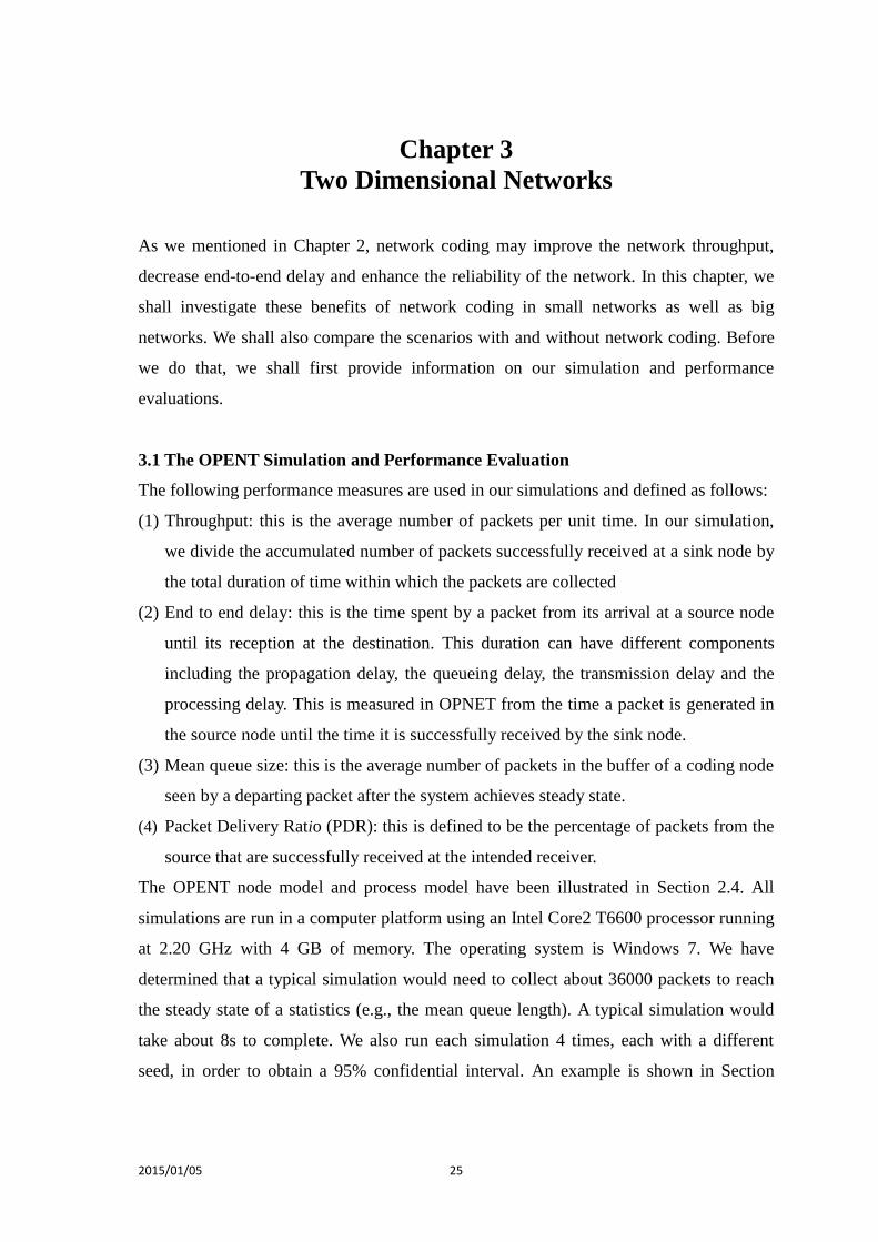
Figure 3.3: End To End Delay vs Arrival Rate, Butterfly Topology
3.2.1.2 ETE Delay
Figure 3.3 is the average end-to-end delay at the sink node as a function of the arrival
rates at the source node when the packet size is fixed at 128 bytes. For the network
without network coding, the delay is first constant with respect to increasing packet
arrival rate, but is building up quickly beyond the packet arrival rate of 4.4 packets/sec.
This can be explained by the D/D/1 behavior because the arrival to the node is modulated
by the departure process of the upstream node. Since the service time of each packet is
fixed, so it would appear that the packets are departing deterministically when the queue
is non-empty (usually at high arrival rates to the node). When the arrival rate increase
beyond the service rate at node C, the system become unstable. For network with NC, we
can see the ETE delay is always lower. The delay is first decreasing with increasing
packet arrival rate because a packet is more likely to find another packet at the other data
stream to perform coding at higher arrival rate instead of waiting for the other packet
when packet arrival rate is very low. Furthermore, the delay remains stable beyond the
packet arrival rate of 4 packets/sec. The “unstable point” beyond which the delay
increases rapidly is now at approximately 9 packets/sec and the delay is ~0.4s. Note that
the delay is lower in the NC scenario because the server only needs to service one coded
2015/01/05 29
packet instead of two original packets.
Figure 3.4 PDR vs. Packet Loss Rate, Butterfly Topology
3.2.1.3 PDR
Figure 3.4 shows the Packet Delivery Rate performance at the sink node as a function of
packet loss rate when the packet size is 128 byte and the packet arrival rate is 2
packets/sec. As we can observe, the PDR is decreasing linearly approximately with
respect to increasing packet loss rate. This is expected as more packets are lost before
arriving at the destination. For network without NC, the PDR is actually higher. This is
because NC in this topology needs to receive all needed packets from the two incoming
streams to decode the original one. However without NC, one lost packet does not affect
the receiving of packets in the other stream.
Figure 3.5: Mean Queue Size vs Packet Arrival Rate, Butterfly Topology
2015/01/05 30
3.2.1.4 Mean Queue Size at the Coding Node
Figure 3.5 is the mean queueing size of the coding node as a function of packet arrival
rate at a source node. The queue size is the total of subqueue0 and subqueue1. For
network without NC, the mean queue size is increasing more or less linearly with respect
to the packet arrival rate, and then rapidly beyond 4 packets/s. This is because the
maximum node service rate is only 9.38 packets/s which is the stability limit of a queuing
system. With two incoming streams, the total arrival rate at the coding node would
exceed 9.38 packets/s if the packet arrival rate at each source is beyond 9.38/2=4.69
packets/s. With NC, the mean queue size is always smaller than network without NC, and
the mean queue size levels off beyond the packet arrival rate of 9 packets/sec. This is
because two traffic streams are combined/coded into one stream and the effective
departure rates of the traffic from the two source nodes (and therefore the arrival rate to
the coding node) will not be higher than its service rate (link bandwidth) and the
departure becomes more constant (fixed service time of a packet). So the queueing at the
coding node behaves more like a D/D/1 system except there is no unstable point even
though the arrival rate at the source can exceed the service rate of the coding node. The
result indicates that using network coding can also decrease the queueing size since it
combines two packets together. It means network coding has more advantages when it
comes to limited node buffer space.
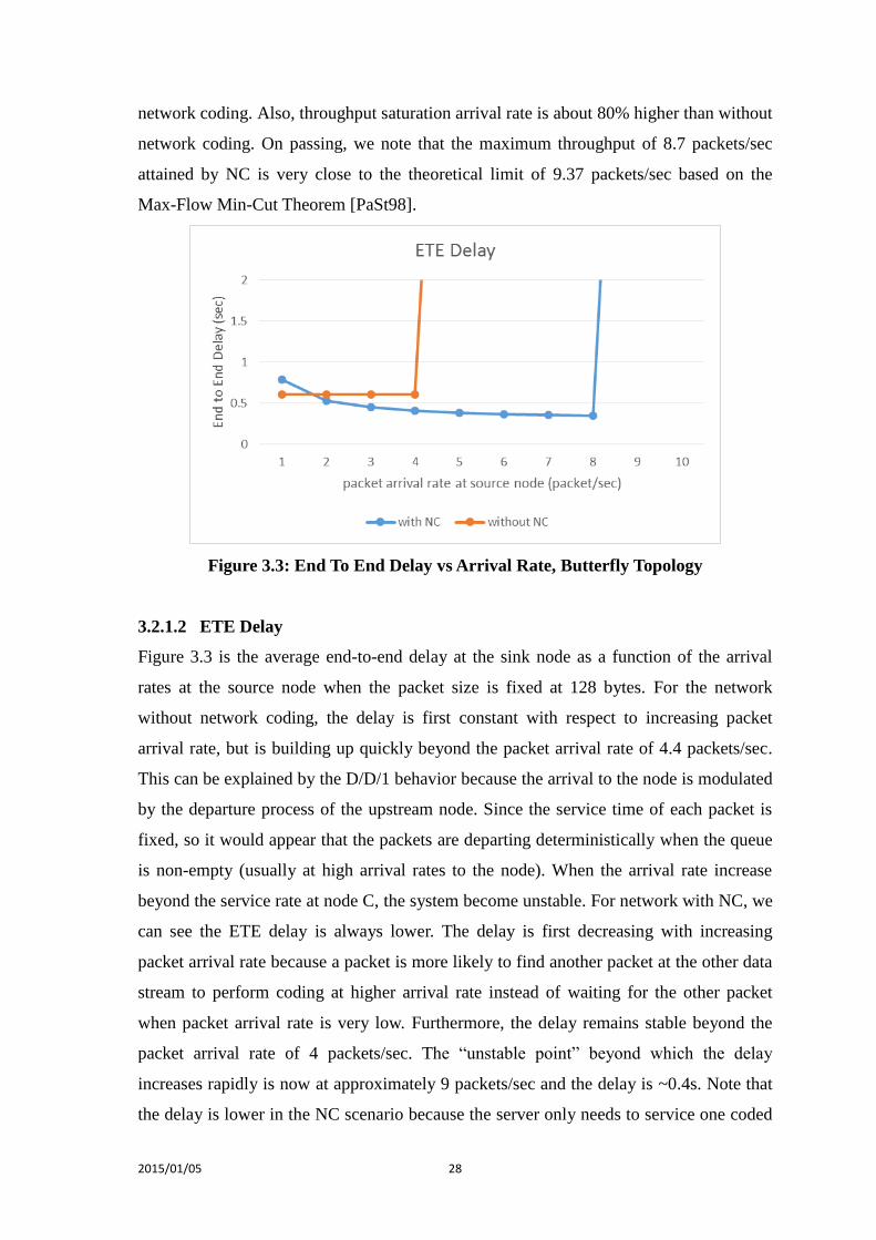
Figure 3.6: Mean Queue Size of Subqueue0
2015/01/05 31
Figure 3.6 shows the queue size of subqueue0 when arrival rate of the two source are
different. Here 𝜆1 is the arrival rate at subqueue0 and 𝜆2 at subqueue1. Each curve has
is a function of the arrival rate 𝜆2 at subqueue1 with arrival rate at subqueue0 fixed at
𝜆1. As we can see from the figure, the queue size of subqueue0 is very large as long as
𝜆2 ≤ 𝜆1. This is because that when 𝜆2 ≤ 𝜆1, many packets from source A must wait for
the packets from source B to perform encoding. When 𝜆2 > 𝜆1, the average queue size
of subqueue0 becomes stable. This is because subqueue1 always has a packet for
encoding when a packet from source A is inserted to subqueue0. For the same 𝜆2, the
queue size of subqueue0 increases with increasing 𝜆1.
Figure 3.7: 95% Confidential Intervals of the Mean Queue Length
Fig.3.7 shows the 95% confidential interval of the mean queue length of the coding node
in the butterfly topology. The intervals are defined by the grey and orange dots with the
mean shown by the blue dots. The interval for each data point is obtained from 4
simulation runs, each with a different seed. As can be seen, the upper and lower bounds
of the confidence intervals are very close to the mean queue size curve. Since all the
other curves have similar observations, we just omit them for all the other curves in this
thesis for clarity reason.
3.2.2 Multi-Relay Topology
Figure 3.8 is the multi-relay topology that we want to compare NC with no NC in a lossy
network. Each of node A and node B serves as both the source and the destination nodes.
All links are bidirectional and with a high probability of losing packets.
In order to transmit a packet from node A to node B, node A would choose one of the
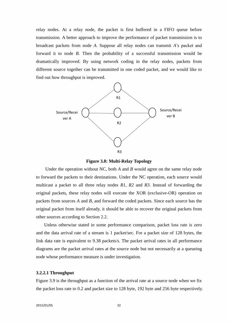
2015/01/05 32
relay nodes. At a relay node, the packet is first buffered in a FIFO queue before
transmission. A better approach to improve the performance of packet transmission is to
broadcast packets from node A. Suppose all relay nodes can transmit A’s packet and
forward it to node B. Then the probability of a successful transmission would be
dramatically improved. By using network coding in the relay nodes, packets from
different source together can be transmitted in one coded packet, and we would like to
find out how throughput is improved.
Figure 3.8: Multi-Relay Topology
Under the operation without NC, both A and B would agree on the same relay node
to forward the packets to their destinations. Under the NC operation, each source would
multicast a packet to all three relay nodes R1, R2 and R3. Instead of forwarding the
original packets, these relay nodes will execute the XOR (exclusive-OR) operation on
packets from sources A and B, and forward the coded packets. Since each source has the
original packet from itself already, it should be able to recover the original packets from
other sources according to Section 2.2.
Unless otherwise stated in some performance comparison, packet loss rate is zero
and the data arrival rate of a stream is 1 packet/sec. For a packet size of 128 bytes, the
link data rate is equivalent to 9.38 packets/s. The packet arrival rates in all performance
diagrams are the packet arrival rates at the source node but not necessarily at a queueing
node whose performance measure is under investigation.
3.2.2.1 Throughput
Figure 3.9 is the throughput as a function of the arrival rate at a source node when we fix
the packet loss rate to 0.2 and packet size to 128 byte, 192 byte and 256 byte respectively.
Source/Recei
ver A
Source/Recei
ver B
R1
R2
R3
2015/01/05 33
For network without NC, one can see that, when packet size is 128 byte, the throughput
is increasing more or less linearly with respect to the packet arrival rate before leveling
off at a throughput of 2.8 packets/sec when the packet arrival rate goes beyond 6
packets/sec. With NC, we can see the leveling off is at a higher throughput of 7.3
packets/sec when the packet arrival rate beyond 8 packets/sec. Note that this maximum
throughput of 7.3 packets/sec using NC is very close to the theoretical limit of 7.4
packets/sec predicted by the Max-Flow Min-Cut Theorem [PaSt98].
Figure 3.9: Throughput vs. Packet Arrival Rate of the Multi-Relay Network
The trends for packet size of 192 byte and 256 byte are similar to the result of 128 byte
except the throughputs are lower (at 5.8 packet/s and 3.6 packets/s respectively) and the
leveling off points occur earlier (when going beyond arrival rates of 6 packets/s and 4
packets/s respectively).
Figure 3.10: ETE delay vs. Packet Arrival Rate of the Multi-Relay Network
2015/01/05 34
3.2.2.2 ETE Delay
Figure 3.10 shows the ETE delay performance as a function of packet arrival rate. For
network without network coding, the end-to-end delay is constant as in a D/D/1 queue
performance until the packet arrival rate reaches 5 packets/sec. The explanation is similar
to that for the butterfly topology in Section 3.2.1.2. After this point, the ETE delay builds
up very quickly because the packet arrival rate is now higher than the service rate of the
network and the network becomes unstable. For the network with NC, the end-to-end
delay is smaller and stable around 0.5s before the packet arrival rate reaches 8
packets/sec. The delay is lower in the NC scenario because the server only needs to
service one coded packet instead of two original packets.
Figure 3.11 PDR vs. Packet Loss Rate, Multi-Relay Topology
3.2.2.3 PDR
Figure 3.11 is the PDR at the sink node as a function of packet loss rates, when the
packet size is 128 byte and the packet arrival rate is 1 packets/sec. For network without
NC, one can see that the PDR decreases more or less linearly with respect to the
increasing packet loss rate. For the network using NC, the PDR performance is less linear
but higher than without NC. This observation is opposite to the Butterfly where NC has
lower PDR. This is because the destination node in the Butterfly network can decode a
packet only when both the coded packet and the original packet from the other link are
received. So a packet cannot be recovered when both packets are lost. In the multi-relay
topology, the destination node is also the source to generate (and therefore known) one of
2015/01/05 35
the original packets that participate in the encoding. Furthermore, since there are three
relay nodes to transmit the coded packets, the probability of losing all three coded
packets is very small. As long as one coded packet is received, the destination can decode
and recover the original packets with a very high probability. Hence the PDR is also
increased.
3.2.2.4 Mean Queue Size of the Coding Node
The mean queue size of the coding node is the same as the one in butterfly topology. This
is because the path setup in this topology (e.g. A-R1-B) can be seen as a butterfly
topology in Fig 2.6 and Fig 2.7. For the purpose of clarity, the performance diagram and
its discussion are omitted here.
3.2.3 Performance Tradeoff and Comparison of the Two Topologies
Summarizing the evaluation results of the Butterfly topology, one sees that without
network coding, the throughput saturates, the ETE delay builds up quickly after the
unstable point, and the PDR decrease with packet loss rate. All these are normally
expected of an ordinary queue. However, NC allows a higher saturation throughput and a
lower ETE delay at the expense of lower PDR performance when the packet loss rate is
present. So it would be good to apply network coding to the Butterfly topology when the
packet loss rate is small.
The observations on the performance tradeoff for the multi-relay network are similar.
One difference is that applying NC in this network gives a higher PDR but at higher cost
of using three relay nodes and transmitting redundancy packets.
We did not evaluate the security performance. However as we mentioned in Ch.2,
one cannot decode the packets until it has a sufficient number of coded packets or
original packets. Even if someone has obtained one coded packet by eavesdropping,
nothing can be done unless enough packets are obtained to decode this coded packet.
Hence, network security using NC would be improved.
3.3 Big Networks
Fig. 3.12 shows a wired network with 2 sources and 2 sinks. Each source node needs to
multicast packets to both sinks T1 and T2. Each sink node is four hops away from the
source node. Each link is unidirectional and has a probability p of dropping packets.
We shall use this topology to compare the network performance with and without NC.
2015/01/05 36
Figure 3.12: Big Network Topology
Figure 3.13a: Big Network without NC Scenario
Figure 3.13a is a scenario when NC is not applied. Each source sets up a data stream to
each sink node and sends the same packets without using network coding. Fixed routing
is achieved by multicasting to specific nodes. Source S1 sends the packets a to relay
nodes A and C only which then forward the packets to the center node E. Similarly,
packets b are sent from source S2 and forwarded to E from relay nodes B and D. Even
though the center node E has 4 downstream nodes, it only multicasts packets a to nodes
F and I which then forward the packets to sinks T1 and T2. Similarly, node E multicasts
packets b only to nodes G and H in order to reach T1 and T2. Note that if the same
packets from both paths are lost (e.g. where both packet a have red slashes), neither sink
nodes T1 or T2 will be able to recover the packets. In this case, NC can alleviate this
2015/01/05 37
situation while maintaining the same throughput as discussed in the following.
Figure 3.13b: Big Network with NC Scenario
Figure 3.13b is the scenario when network coding is applied. Each of the source nodes S1
and S2 broadcasts their packets a and b to relay nodes A, B, C and D. These relay nodes
are the first-level coding nodes that would code packets from streams a and b together
using linear encoding and generate four different coded packets Y1, Y2, Y3 and Y4. Each
relay node would then forward its coded packets to the center node E. Node E is the
second-level coding node which recode two of the packets it received (discard others) to
generate four new coded packets Z1, Z2, Z3 and Z4. Each of these is then unicast to relay
nodes F, G, H and I, respectively which in turn multicast to both sink nodes T1 and T2.
Each of the two sink nodes would decode the packets using the decoding algorithm
described in Section 2.2
According to the discussion in Section 2.2, each of the first-level coding nodes (A, B,
C or D) uses the linear encoding algorithm with m=2 and n=1. The second-level
encoding node E uses m=2 and n=4 for the encoding algorithm. Since there can be up to
4 subqueues in the coding buffer, node E can just pick any two randomly (In our
implementation, we simply pick in the order to the subqueue IDs, i.e., subque0, subque1,
subque2 and subque3 if the subqueues are non-empty. Finally, each of the decoding node
(T1 or T2) decodes the packets using m=N(s) =2. A packet can be decoded if N(g)2.
Under the same loss scenario in Fig. 3.11b, one can see that the two sink nodes can
recover the original packets. This is because each sink node is able to decode its packet
Z1
Z4
2015/01/05 38
stream as long as it has received two arbitrary coded packets as per discussion in Section
2.2 So with network coding, the network robustness is improved without using more
packets to the network.
3.3.1 Performance Evaluations
We shall evaluate the performance in terms of throughput, ETE delay and PDR. Unless
otherwise stated in some performance comparisons, packet loss rate is 0.2 and data
arrival rate of a stream is 1 packet/sec. The packet size is 128 bytes. For a default link
data rate of 9600bps, this is equivalent to 9.38 packets/s. The packet arrival rates in all
performance diagrams are packet arrival rates at the source node but not necessarily at a
queueing node (e.g., relay or sink) whose performance measure is under investigation.
Figure 3.14a: Throughput with Different Packet Size, Big Network
3.3.1.1 Throughput
Figure 3.14a is the throughput seen at a sink node (both T1 and T2 are symmetrical in
performance) as a function of the packet arrival rate at the source node when packet size
is set to 128 byte, 196 byte and 256 byte, respectively. For a network without NC and
using a packet size of 128 byte, the throughput is increasing more or less linearly with
respect to the increasing packet arrival rate before leveling off at 3.8 packets/sec beyond
a packet arrival rate of 8 packets/s. By using NC, one can see the throughput can level off
at a higher level of 6.2 packets/sec and beyond a higher packet arrival rate of 9
packets/sec.
2015/01/05 39
The trends for packet sizes of 192 byte and 256 byte are similar to the result for a
packet size of 128 byte, except that the maximum throughputs are lower and the leveling
off point occurs earlier. In scenario without NC, the throughputs level off at 2.5
packets/sec and 2.1 packets/sec respectively, when arrival rates go beyond 5 packet/sec
and 4 packets/sec respectively. In scenario with NC, the throughputs levels are 4.2
packets/sec and 3.2 packets/sec respectively for arrival rates beyond 6 packet/sec and 5
packets/sec respectively. The maximum throughput obtained by Max-Flow Min-Cut
[PaSt98] theory is 7.44 packets/sec for this network, which is almost achieved by NC.
Figure 3.14 b: Throughout vs. Packet Arrival Rate in a Big Network
Figure 3.14b is the throughput seen at a sink node (both T1 and T2 are symmetrical in
performance) as a function of the packet arrival rate at source node in the big network
with different packet loss rates in a link. When the packet loss rate is 0.2, the network
throughput without NC is increasing more or less linearly with respect to the increasing
packet arrival rate before leveling off at 3.6 packets/s beyond the packet arrival rate of 7
packets/sec. Using NC, one can see the leveling off occurs at a higher level of 6.2
packets/s and beyond a higher packet arrival rate of 9 packets/sec. The maximum
throughout achieved by NC is about twice that of network without NC. The trends for
packet loss rate of 0.1 is similar to the result of packet loss rate of 0.2. Without NC, the
throughput is leveling off at 4 packets/sec beyond the packet arrival rate of 9 packets/sec.
By using NC, the throughput is leveling off at 8 packet/sec when packet arrival rate goes
beyond 9 packets/sec. There is a drop at the packet arrival rate of 8 packet/sec for no NC.
2015/01/05 40
This is due to too many packets injected into the network when the loss rate is low, and
the network has encountered traffic congestion. However, this situation does not happen
with NC, because network coding can also reduce traffic load in the network.
Figure 3.15: ETE delay vs. Packet Arrival Rate in a Big Network
3.3.1.2 ETE Delay
Figure 3.15 shows the end-to-end delay at the sink node as a function of the packet
arrival rates. For network without NC with loss rate fixed at 0.2, the ETE is constant until
the packet arrival rate reach 6 packets/sec. The explanation is similar to that for the
butterfly topology in Section 3.2.1.2. With NC, the ETE delay is slightly higher, but it
builds up at a higher packet arrival rate of 8 packets/sec. When the packet loss rate is 0.1,
the observations and comparison are similar except the delay shoot-up points are 5
packets/s (without NC) and 8 packets/s (with NC). Note that the delay curve shoots up as
the system is approaching its service limit of 9.38 packets/s. In summary, NC can handle
a higher packet arrival rate, especially when the packet loss rate is low.
Note also that we have not considered the retransmission of a lost packet. Without
NC the sink is not able to recover a lost packet. Therefore, the ETE delay for network
without NC would be even more if one includes the retransmission time to recover a lost
packet.
2015/01/05 41
Figure 3.16: PDR vs. Packet Loss Rate of a Big Network
3.3.1.3 PDR
Figure 3.16 is the PDR performance of the big network as a function of the packet loss
rates in percentage. For network without NC, the PDR is a decreasing function of packet
loss rate although the PDR is only decreasing slowly for packet loss rate < 1%. Note that
PDR cannot achieve 100% (not shown) even if the packet loss rate is very small (~0%)
because the sink node is not able to recover a lost packet. But with NC, the network can
achieve 100% successful packet delivery when the packet loss rate is below 5%. When
the packet loss rate increases to 40%, the PDR of both methods are very low due to too
many packets lost in the network.
Figure 3.17: Mean Queue Size of a Big Network
2015/01/05 42
3.3.1.4 Mean Queue Size
Figure 3.17 is the mean queue size at one of the relay (also first-level coding) nodes A, B,
C or D as a function of packet arrival rate at a source node. The mean queue size is the
sum of two subqueues. For network without NC, the mean queue size increases linearly
before it leveling off at a packet arrival rate of 9 packets/sec. The reason for the leveling
off is due to the modulating effect of the source node as explained in Section 3.2.1.4
earlier. With NC, the mean queue size is higher. However, it levels off at the mean queue
size of 2 packets beyond the packet arrival rate of 9 packets/sec. The reason is again the
modulating effect from the source. The departure rate of the traffic from the source node
(and therefore the arrival rate to the relay/coding node) will not be higher than its service
rate (link bandwidth) and the departure becomes more constant (fixed service time of a
packet). So the queueing at the coding node behaves more like a D/D/1 system except
there is no unstable point even though the arrival rate at the source can exceed the service
rate of the coding node. The same observation and explanation would apply to the
network with network coding except the queue size.
3.3.2 Performance Tradeoff
Summarizing the evaluation results from the big network topology, one can see that
without network coding, the throughput increases with arrival rate, and the ETE delay
shoots up after an unstable point and the PDR would decrease with packet loss rate, as
normally expected of an ordinary queue. However, NC allows a higher throughput
saturation and PDR levels but at the expense of a higher ETE delay as well as a higher
mean queue size at the relay node even when the packet arrival rate is small. So network
coding is good to this big network topology when packet arrival rates and packet loss
rates are higher.
On the other hand, the ETE delay using NC is a little bit higher than without NC
scenario when packet arrival rates are low. This is due to the overhead in producing
duplicates where we need to produce 4 packets at one source node to broadcast to 4 relay
nodes. Therefore the sink node need to receive 4 packets, one each from 4 relay nodes F,
G, H and I. Without NC, the sink node needs to receive two only.
3.4 Concluding Remarks
Comparing the small networks (Section 3.2) and big networks (Section 3.3), the trends of
the performance curves are essentially the same except for some congestion phenomenon
2015/01/05 43
(as discussed in Fig. 3.12b) that can arise in big networks. For big network using NC, the
ETE delay is a little bit higher than small networks (using NC) because one would need
to transmit more packets to relay nodes, and the PDR performance of the big network is
also better because one can decode the original packets by any two coded packets. Other
than this, one can readily see from this chapter that NC can achieve better throughput,
ETE delay and network reliability (PDR). As commented in different sections, NC can
achieve close to the maximum throughput possible allowed/predicted by the Max-Flow
Min-Cut Theory. With our experience from this chapter, we are now ready to apply NC
to an underwater network which has a more challenging environment.
2015/01/05 44
Chapter 4
3D Underwater Network
Chapter 3 has demonstrated the capability of network coding to improve the network
performance. We shall now investigate its potential for the underwater network as an
application. It also expands the scope to a three-dimensional network as opposed to those
two-dimensional ones in the last chapter. To do proper simulation and evaluation, we
shall first review/summarize the mathematical model for the underwater wireless
channels which is quite different from the air wireless channel. This model is then used to
revise the OPNET radio pipelines in order to match the unique underwater channel. After
that, we shall carry out OPNET simulation to evaluate the performance of an underwater
network with a cube topology in terms of throughput, delay, power, SNR (Signal Noise
Ratio) and network reliability.
4.1 Underwater Channel Characterization For OPNET Design
As mentioned in our review, acoustic waves are used due to its better transmission rate
(albeit low) in underwater wireless communication. Here, we shall review below the few
special features of the underwater acoustic waves and their characteristic equations for
the design of OPNET pipeline stages in order to match the underwater channel.
(1) Propagation delay
The long propagation delay is a principle feature of underwater networks. Unlike the
2x10^8 m/s of light wave energy in air, the acoustic wave propagation speed x in water is
only 1500 m/s. Therefore, to travel a distance d, we need to change the formula of
propagation delay =d/ x.
(2) Path loss [AkPo05, RBMa11]
The path loss mainly includes attenuation and geometric spreading. The attenuation
arises from the absorption and conversion of acoustic energy into heat. The signal power
decreases within the transmission channel between the source and the sink. The
attenuation becomes larger at a longer distance and at a higher frequency. Geometric
spreading means the spreading of sound energy as a result of the expansion of the
acoustic wave fronts. It increases with the propagation distance and is independent of
frequency. The general path loss A(k,d) in a underwater channel is [SoSt00]
A(k,d)=𝑑𝑘𝑎𝑑 (4.1)
2015/01/05 45
where d is the transmission distances in Km; k is the energy spreading factor (1 for
cylindrical, 1.5 for practical, and 2 for spherical spreading) [SoSt00]; and a is the
abortion coefficient. The abortion coefficient depends on the signal frequency, and it is
computed according to Thorp’s empirical formula [SoSt00]:
10 log(a) = 0.11𝑓2
1+𝑓2 + 44𝑓2
4100+𝑓2 + 2.75 ∗ 10−4𝑓2 + 0.003 (4.2)
where f in kHz is the signal frequency Tx_center_freq discussed below.
(3) Transmission channel bandwidth.
The available bandwidth for underwater acoustic waves channel is very limited. The
bandwidth is inversely proportional to the propagation distance. For long underwater
transmission distance, the bandwidth is limited to the order of KHz. This is often used as
the transmitter bandwidth (tx_bandwidth) in the following transmitter center frequency f
given by
f=Tx_center_freq=tx_base_freq+ 𝑇𝑥_𝑏𝑎𝑛𝑑𝑤𝑖𝑑𝑡ℎ
2.0 (4.3)
where tx_base_freq is the base frequency of the transmitter power stage.
(4) Receiver power
The receiver power Pr is obtained by
𝑃𝑟 = 𝑃𝑡 ∗ 𝐴 (4.4)
where 𝑃𝑡 is transmitter power, and A is the path loss given above.
(5) Noise
The underwater noise includes the ambient noise and the man-made noise (e.g., those
caused by machines) [RBMa11]. There are different types of ambient noise whose values
can be obtained by the empirical formula of the Wenz model [CoFW90] as follows.
a) The turbulence noise 𝑁𝑡 given by 10 log 𝑁𝑡(𝑓) = 17 − 30𝑙𝑜𝑔𝑓
b) The shipping noise 𝑁𝑠 given by 10 log𝑁𝑠(𝑓) = 40 + 20(𝑠 − 0.5) + 26𝑙𝑜𝑔𝑓 −
60log (𝑓 + 0.03) where s is the shipping factor between 0 and 1.
c) The wind-driven wave noise 𝑁𝑤 given by 10log𝑁𝑤(𝑓) = 50 + 7.5𝑤0.5 +
20𝑙𝑜𝑔𝑓 − 40 log(𝑓 + 0.4) where w is the wind speed in m/s.
d) The thermal noise 𝑁𝑡ℎ for the radio transmitter given by 𝑁𝑡ℎ =(rx_temp +
bkg_temp)*rx_bandwidth*BOLTZMANN. where rx_temp is the receiver temperature,
bkg_temp is the effective background temperature, rx_bandwidth is the receiver
bandwidth and BOLTZMANN is Boltzmann constant of 1.379*10−23J/K.
In our investigation, we shall only consider the ambient noise which can vary with
the position and the frequency. The total ambient noise directly affects the SNR at the
2015/01/05 46
receiver, the power of the transmitter and the carrier frequency of the transmission signal.
We shall assume the man-made noise to be zero to maximize the SNR. So the total noise
power is due to the sum of all ambient noise components which is given by
𝑁𝑎𝑙𝑙 = 𝑁𝑡+𝑁𝑠+𝑁𝑤+𝑁𝑡ℎ
We have used this noise power to modify the background noise pipeline stage of OPNET.
In summary, all the above factors will contribute to a lower SNR at the receiver, and
therefore a lower data rate for the communication channels according to Shannon’s
Theorem [TaSc86]. Due to the multipath propagation and various noise factors, the
underwater channel may experience a high bit error rate. Accordingly, the packet loss rate
is also higher when compared with terrestrial channels as well as the probability of losing
connectivity.
Figure 4.1: The 3D Underwater Network
4.2 The 3D Network Topology
Figure 4.1 shows the three dimensional topology we shall study for the underwater
environment. The 3*3*3 topology consists of 27 nodes. Each node is a wireless node and
has the same communication radius. Suppose that node N1 needs to transmit packet B to
node N12 which is 6 hops away, and that Node N4 needs to transmit packet A to node
N10. Their data transmission paths are indicated by the color arrows in the figure: red for
packets A and green for packets B. Let Node N3 be the coding node that will perform the
2015/01/05 47
XOR operation on packets A and B. After encoding, N3 transmits the coded packets to
node N10 and N12 through the paths indicated by the white arrows. One can see that
such coding topology is effectively a modified butterfly network as illustrated in Section
2.3.
4.2.1 Network Parameters
For the physical channel shown in Fig. 4.1, we shall use the parameters shown in Table
4.1 below.
Table 4.1: Parameters for Underwater Sensor Network
acoustic speed 1500m/s
data rate 1024bps
link length 100m
Packet size 1024 bit
tx_base_freq 30kHz
tx_bandwidth 20kHz
We also use k=2 for spherical diffusion of the acoustic wave. Using the above parameter
values, one can obtain the center frequency f = 40Khz from eqn. (4.3), the abortion
coefficient a= 0.025 from eqn. (4.2), and the path loss A = 0.05 from eqn. (4.1). We shall
also use a transmitter power Pt = 100W, the BPSK (Binary Phase Shift Keying) digital
modulation, and the temperatures of bkg_temp=290K, rx_temp=290K. All these
settings and calculations are used as the parameter values (e.g., the bit error rate) of the
pipeline stages discussed in Section 2.4.3
At the network layer level, we consider a constant packet arrival rate that can vary
from 1 packets/sec to 10 packets/sec depending on the scenario under investigation. The
packet size is constant at 1024 bits. The data rate of the channel is set to 1024 bps to
match the low data rate of underwater channel.
4.3 Performance Evaluation
We shall use OPNET simulations to evaluate the performance of the underwater cube
network in terms of throughput, end to end delay and PDR. The packet arrival rates in all
diagrams are at the source node.
2015/01/05 48
Figure 4.2: Underwater Network Throughput
4.3.1 Throughput
Figure 4.2 is the throughput of the underwater “butterfly” network as a function of
packet arrival rate at a source node when packet size is fixed at 128 byte, 192 byte and
256 byte respectively. For the scenario without NC and a packet size of 128 byte, the
throughput is increasing linearly with the respect of packet arrival rate before levelling
off at the throughput of 0.45 packets/sec when the data rates go beyond 0.7 packets/sec.
This is because the low channel capacity of underwater network. By using network
coding, the leveling off reaches a higher throughput of 1 packets/sec and beyond a larger
packet arrival rate of 0.5 packet/sec. The trends for packet sizes of 192 byte and 256 byte
are similar to the results for packet size is 128 byte, except the throughputs are lower and
the leveling off points are earlier. In the scenario without NC, the leveling off points are
at throughput of 0.2 packets/sec and 0.18 packets/sec respectively, for packet arrival rates
going beyond 0.3 packets/sec and 0.2 packets/sec respectively. In the scenario with NC,
the saturation points are at throughput of 0.64 packets/sec and 0.4 packets/sec
respectively, when packet arrival rates go beyond 0.6 packets/sec and 0.4 packets/sec
respectively.
2015/01/05 49
Figure 4.3: Underwater End to End Delay
4.3.2 ETE Delay
Figure 4.3 is the end-to-end delay as a function of packet arrival rate at the source node
of the underwater butterfly network. For the scenario without NC, the delay is constant as
a D/D/1 queue behavior before the packet arrival rate goes beyond 0.4 packets/sec. The
reason is similar to that for the butterfly topology in Section 3.2.1.2. By using NC, this
critical point has increased to 0.9 packets/sec and the ETE delay of the network is
slightly better than that without network coding, but not very notable.
Figure 4.4 PDR, Underwater Network
2015/01/05 50
4.3.3 PDR
Figure 4.4 shows the PDR as a function of packet loss rate in the underwater network.
For network without NC, one sees that the PDR is a decreasing function (more or less
linearly) with increasing packet loss rate. One sees that the PDR is more than halved
when packet loss rate exceeds 25%.
For the network with NC, the PDR is basically the same. This is because only XOR
coding is used in this network. If the coded packet is missing, the sink node cannot
decode the original packets. It is the same in the scenario without NC, the sink cannot
receive a packet if it is lost in the transmission.
4.3.4 Comparison with Terrestrial Networks
Comparing with terrestrial networks in Ch.3, one can see the following changes in the
performance measures of the underwater network:
1) The ETE delay has increased to 10-20 seconds due to the high propagation delay.
2) The maximum packet arrival rate which can be achieved is much lower than the
terrestrial networks. For a packet size of 128 byte used in the terrestrial networks in
Chapter 3, the maximum packet arrival rate can reach 8 or 9 packets/sec (with NC).
For the underwater network, the packet arrival rate can only achieve 1 packets/sec.
3) Throughput is much lower than the terrestrial network due to the low data rate. For a
packet size of 128 byte used in the terrestrial networks in Chapter 3, the maximum
throughput could achieve 8.7 packets/sec.
4.4 Concluding Remarks
In this chapter, we have applied NC to the 3D butterfly topology of an underwater
network. In order to truly simulate the underwater environment, we have modified
several channel characteristics in the OPNET pipeline stages. From the simulation results,
we could see that the performance of NC in the underwater network is not so promising
when compared to the terrestrial network as exhibited by the high delay and the low
maximum throughput. Much improvement is desirable.
2015/01/05 51
Chapter 5
Design Issues and Guidelines
We shall discuss in this chapter some design issues we have encountered in our research
procedure and give a guideline to the design of network using network coding. Based on
our design and simulation experience, we shall provide some recommended parameters
to obtain a better network performance.
5.1 Choice of Topologies
Choose a suitable topology and appropriate coding nodes can make a better use of
network coding. Network coding requires one to identify a topology during the design
stage. We should know the number of network nodes, their connectivity and functions so
that the coding nodes can be located. Some topologies do not improve network
performance remarkably with network coding such as the peer-to-peer topology
[WaLi06]. Choosing the proper network topology and an appropriate coding node to
perform network coding can reduce the complexity of the network and decoding process.
Based on our experience, one should look for networks with bottleneck links. We
can then use network coding to decrease the number of packets transmitted in the
bottleneck links and balance the information flows to other unused links. The other
suitable topology type is networks with multiple relay nodes, especially those with high
loss rate links. The reliability of the network would be significantly improved by
transmitting different coded packets generated by different coding coefficients.
Note that the regular and symmetric networks we studied here is not a necessary
requirement. It is just a condition that would facilitate network coding as used by many
researchers.
5.2 Coding and Decoding Complexity
The XOR coding algorithm is the simplest coding and decoding method we would
recommend for bottleneck network to improve the throughput performance. But it is not
good enough to improve the probability of decoding the original packets in high loss
networks. Linear coding is recommended instead. In practical networks, we should
choose the properly coding algorithm according to its network characteristic and
applications. For small networks, simple fixed coding is recommended to decrease the
2015/01/05 52
coding complexity. For big networks especially random networks, linear coding is
recommended to generate independent linear combinations of the original packets; the
robustness of the network will be remarkable improved.
Another issue we need to consider is the number of packets to be coded together. This is
because the destination node has to buffer the same number of coded packets before it
can decode the original packets. If the number of packets for the same generation is too
big, the decoding complexity would become very high, e.g. Ω(ℎ2𝑘), where h is the
number of packets to be delivered and k is the number of receivers [LaSp06].
5.3 Tradeoff
Based on the simulation experience in Chapter 3, network coding does not always
improve the network performance. For example, the ETE delay in the Big Network
section is higher when using NC, and the PDR is lower in Butterfly Network when using
NC. Therefore, we should consider different network coding methods according to the
specific requirement. In some cases, the improvement may not be noticeable for some
parameter settings. In the Butterfly topology in Section 3.2.1, the throughput saturation is
higher and ETE delay is lower, but at the expense of a lower PDR. In the multi-relay
network in Section 3.2.2, the throughput, the ETE delay and the PDR are all better when
using NC but at the expense of using more relay nodes. In the big network case in
Section 3.3, the throughput and the PRD performances are better but at the expense of
higher ETE delay. In the underwater network in Ch.4, the PDR performance is also not
improved.
As one would observe from Chapter 3 and Chapter 4, the maximum arrival rate one
can tolerate before everything becomes bad is just the service rate of the outgoing link.
This is well understood from queueing theory. For network with NC, the maximum
arrival rate would achieve as twice as the service rate.
5.4 Limitations
We have observed some interesting limitations/disadvantages of network coding during
our research. Take the case in Section 2.2.1 as an example, it is commented that one
packet stream may have to wait for the packet arrivals from another packet stream to
perform network coding. This would increase the delay performance if the buffer of the
other stream is often empty. This can often happen when one data stream as a lower
arrival rate than the other, which is further illustrated and discussed in Fig.3.6 of Section
2015/01/05 53
3.2.1.3. So a designer can be limited to using the same arrival rates for streams
performing NC. Different approaches must be used to resolve this issue and their
performances studied. For example, one can use “packet do not wait at the coding node”.
If there is no packet to code with, send the original packet without NC right away, and
see the different performance.
2015/01/05 54
Chapter 6
Conclusions
We have studied several symmetric topologies with network coding operation in this
thesis. We have conducted many simulations to evaluate the performance under different
scenarios using different parameters. Our results have confirmed that network coding has
the potential of improving the performances of network throughput, end-to-end delay and
reliability. Meanwhile, we have also analyzed the tradeoffs and drawn a conclusion that
network coding is not always advantageous. It may not be effective or the performance
may become worse under some conditions.
We have modified the wireless channel in OPNET by using parameters to reflect the
underwater characteristics. This has allowed us to use OPNET simulation to study the
underwater acoustic network with network coding. The results indicate that network
coding would increase the throughput and decrease the end to end delay of underwater
acoustic network. However, the PDR does not appear to be good.
Much time was spent in establishing the network model and the underwater channel
mode, in the incorporation of channel coding operation with respect to the topologies, as
well as in the debugging to ensure the correct operation of our simulations. Then many
simulations ensue, followed by the analysis of the network behavior. We have eventually
learned some debugging techniques such as trace instructions from OPNET. Not only we
can use it to follow the path of a packet, but also study the detail operation of a process.
It is easier to identify the location and reason of the problems. Some of these can be
summarized in the lessons we have learned from our OPNET experience. First, one
should be careful about the Transit conditions. OPNET is event-driven and some events
are triggered by the Transit conditions. Many errors are caused by the inappropriate
conditions for transitions. So one needs to consider all possibilities when adapting an
existing process for use in the project. Secondly, one should refer the OPNET User
Manual for help when encountering difficulties. The OPNET User Manual provides the
explanation for every details and also has plenty of examples for you to consult. Lastly,
one can modify the pipelines to match the unique environment. Some characters of the
channel in underwater environment are not the same as terrestrial radio channel. We are
happy to learn this approach to modify the physical transmission channel which is very
useful to evaluate networks of different physical nature in future.
2015/01/05 55
6.1 Future Works
Our work represents the first CCNR investigation of network coding capabilities. Due to
limited time, there are still issues/limitations that need to be investigated. The following
is a non-exhaustive list.
1) The investigation of the “must-wait” phenomenon of the stream with higher data rate
mentioned in Ch.5, and its solutions.
2) Network coding on random topologies as opposed to fixed topologies studied in this
thesis.
3) Incorporating routing to facilitate network coding.
4) Choose a suitable topology and appropriate coding nodes to make better use of network
coding. Determine the criteria to choose the “best” topology for NC.
5) Using logical topologies for NC.
6) A coding method that can improve the PDR performance in an underwater network.
7) NC performance on a Wheel topology.
8) Performance evaluation of network coding in higher protocol layers like TCP.
9) Apply NC to mobile networks.
10) Using random linear coding to different topologies.
11) Evaluate the bandwidth usage in network coding.
2015/01/05 56
References
[AhCa00] R. Ahlswede, Ning Cai,Shuo-Yen Robert Li and Raymond W. Yeung, "Network
information flow," IEEE Transactions on Information Theory, vol. 46, pp. 1204-1216,
2000.
[AkPo05] Ian F. Akyildiz, Dario Pompili and Tommaso Melodia, “Underwater acoustic sensor
networks: research challenges”, Ad Hoc Networks, Vol.3(3), pp.257-279, 2005.
[AlAh09] Osameh M. Al-Kofahi and Ahmed E. Kamal, "Network Coding-Based Protection of
Many-to-One Wireless Flows", IEEE Journal on Selected Areas in Communications,
Vol. 27, No. 5, pp. 797-813, June 2009.
[AyAz11] Muhammad Ayaz, Abdullah Azween, and Ibrahima Faye . “A Survey on Routing
Techniques in Underwater Wireless Sensor Networks”, Journal of Network and
Computer Applications, Vol.34, pp.1908-1927, 2011.
[BiMo05] Sanjit Biswas and Robert Morris, “ExOR: Opportunistic MultiHop Routing for Wireless
Networks”, Proceeding of the 2005 conference on Applications, technologies,
architectures, and protocols for computer communications , pp. 133-144, New York,
2005.
[CaYe10] Ning Cai and Raymond Yeung, “Secure Network Coding on a Wiretap Network”, IEEE
Transactions on Information Theory, Vol.57, pp.424-pp.435, December 2010.
[ChCh10] N. Chirdchoo, Mandar Chitre, and Wee-Seng Soh . "A Study on Network Coding in
Underwater Networks," Proceeding of IEEE, Oceans 2010, pp.1-8, Seattle, WA,
September 2010.
[ChJe07] Szymon Chachulski, Michael Jennings, Sachin Katti and Dina Katabi. “Trading
Structure for Randomness in Wireless Opportunistic Routing”, Proceeding of the 2007
conference on Applications, technologies, architectures, and protocols for computer
communications, pp.169-180, New York, 2007.
[FrBo06] C. Fragouli, J. Boudec, and J. Widmer, “A Network coding: An instant primer”, ACM
SIGCOMGCOMM Computer. Communication. vol. 36, no. 1, pp. 63–68, Jan. 2006.
[GaGo13] Chong Cao, Ping Gong and Li Chou, “Random Network Coding Based The Effective
Wireless MAC Protocol”, Proceeding of 2013 4th IEEE International Conference on
Software Engineering and Service Science (ICSESS), pp.393-396, Beijing, May 2013.
[GhTo08] Majid Ghaderi, Don Towsley and Jim Kurose, “Reliability Gain of Network Coding in
Lossy Wireless Networks”, The 27th Conference on Computer Communications, IEEE.
Phoenix, 2008.
[GuXi06] Zheng. Guo, Peng Xie, Junhong Cui and Bing Wang, "On Applying Network Coding to
Underwater Sensor Networks," presented at The First ACM International Workshop on
UnderWater Networks (WUWNet'06), Los Angeles, California, USA, 2006.
[GuLi10] Bin Guo, Hongkun Li, Chi Zhou, and Yu Cheng, "General Network Coding Conditions
in Multi-Hop Wireless Networks", Proceeding of IEEE International Conference on
Communication (ICC 2010), Cape Town, South Africa, May 2010.
[GuWa09] Zheng Guo, Bing Wang, Peng Xie, Wei Zeng and Jun-Hong Cui "Efficient Error
Recovery Using Network Coding in Underwater Sensor Networks," Elsevier Ad Hoc
Networks, Special Issue on Underwater Networks. vol. 7, no. 4, ed, 2009, pp. 791--802.
[HaZh08] Song Han, Zifei Zhong, Hongxing Li, Guihai Chen, Edward Chan and Aloysius K. Mok,
“Coding-Aware Multi-path Routing in Multi-Hop Wireless Networks”, Proceeding of
IEEE International on Performance, Computing and Communications Conference,
(IPCCC) 2008, pp.93-100, Austin, Texas, Dec. 2008.
[HoMe03] T. Ho, M. Medard, J. Shi, M. Effros, and D. R. Karger, “On randomized network
coding”, Proceedings of 41st Ann. Allerton Conf. Commun., Control Comput., vol.36,
no.1, Urbana-Champaign, IL, Oct. 2003, pp. 63–68.
2015/01/05 57
[IqDa11] Muhammad Azhar Iqbal, Bin Dai, BenxiongHuang, A.Hassan and ShuiYu. “Survey of
network coding-aware routing protocols in wireless networks”, Journal of Network and
Computer Applications, Vol.34(6), pp.1956-1970, 2011.
[KaRa08] Sachin Katti, Hariharan Rahul, Wenjun Hu, Dina Katabi, Muriel Médard and Jon
Crowcroft. “XOR in the Air: Pratical Wireless Network Coding”, IEEE/ACM
Transactions on Networking, Vol.16 (3), pp.497-510, June 2008.
[KeAt89] Kendall Atkinson, “An Introduction to Numerical Analysis”, pp.508-522, New York:
John Wiley & Sons, 1989.
[KeKe13] Veronika Kebkal, Oleksiy Kebkal and Konstantin Kebkal . “Network Coding for
Underwater Acoustic Sensor Networks”, Proceeding of MTS/IEEE, OCEANS 2013,
pp.1-5, Bergen, June 2013.
[KoWa10] Dimitrios Koutsonikolas, Chih-Chun Wang and Y. Charlie Hu, “CCACK: Efficient
Network Coding Based Opportunistic Routing Through Cumulative Coded
Acknowledgments”, IEEE/ACM Transactions on Networking (TON) Archive, Vol. 19,
Issue 5, pp. 1368-138, October 2011.
[Ksch12] Frank R. Kschischang, “An Introduction to NetworkCoding”, pp. 51-60, Elsevier Inc,
2012.
[LaSp06] Michael Langberg and Alex Sprintson, “The encoding complexity of network coding”,
IEEE/ACM Transactions on Networking (TON) - Special issue on networking and
information theory, Vol.14 Issue SI, pp. 2386-2397, June 2006.
[LiLi05] Zongpeng Li, Baochun Li, Dan Jiang and Lap Chi Lau, “On achieving optimal throughput
with network codingng”, Proceeding of IEEE INFOCOM, vol. 3. Miami, FL,
pp. 2184–2194, March 2005.
[LiYe03] Shuo-Yen Robert Li and Raymond W. Yeung, “Linear Network Coding”, IEEE
Transections On Information Theory, VOL. 49, NO. 2, February 2003
[LuMe07] D. E. Lucani, Muriel Medard and Milica Stojanovic, "Network coding schemes for
underwater networks:the benefits of implicit acknowledgement," Proceeding of The Second
Workshop on Underwater Networks , Montrea l , Quebec , Canada, 2007 .
[MaMi13] Claude Manville, Abdulaziz Miyajan and et al. “Network Coding in Underwater Sensor
Networks”, Proceeding of MTS/IEEE, OCEANS 2013, pp.1-5, Bergen, June 2013.
[MoZh12] Haining Mo, Zhong Zhou Ayman Alharbi, Haining Mo, Michael Zuba and Jun-Hong
Cui . “Practical Coding-based Multi-hop Reliable Data Transfer for Underwater
Acoustic Networks”, Proceeding of IEEE Global Communications Conference
(GLOBECOM 2012), pp. 5751-5756, Anaheim, CA, Dec. 2012.
[NaYu10] Tebatso Nage, F. Richard Yu and Marc St-Hilaire, "Adaptive Control of Packet
Overhead in XOR Network Coding", Proceeding of IEEE International Conference on
Communication (ICC 2010), CapeTown, South Africa, May 2010.
[NgTr09] Dong Nguyen, Tuan Tran, Thinh Nguyen and B. Bose, "Wireless Broadcast Using
Network Coding", IEEE Transactions on Vehicular Technology, Vol. 58, No. 2,
pp. 914-925, Feb. 2009.
[NiSa06] Bin Ni, Naveen Santhapuri and Zifei Zhong and Srihari Nelakuditi, “Routing with
Opportunistically Coded Exchanges in Wireless Mesh Networks”, Proceeding of
WiMesh 2006. 2nd IEEE Workshop, pp.157-159, Reston, VA, 2006.
[PaCh10] Parimal Parag and Jean-Francois Chamberland, “Queueing Analysis of a Butterfly
Network for Comparing Network Coding to Classical Routing”, IEEE Transactions on
Information Theory, VOL. 56, NO. 4, April 2010.
[PaHe12] Raul Palacios, Janus Heide, Frank H.P. Fitzek and Fabrizio Granelli, “Design and
Performance Evaluation of Underwater Data Dissemination Strategies using Interference
Avoidance and Network Coding”, IEEE International Conference on Communications
(ICC), pp. 1410 – 1415, Ottawa, June 2012.
2015/01/05 58
[PaSt98] Christos H. Papadimitriou and Kenneth Steiglitz, "6.1 The Max-Flow, Min-Cut
Theorem". Combinatorial Optimization: Algorithms and Complexity. Dover
Publications. pp. 120–128, 1998.
[RaSe08] Shravan Rayanchu, Sayandeep Sen, Jianming Wu, Suman Banerjee and Sudipta
Sengupta“Loss-Aware Network Coding for Unicast Wireless Sessions: Design,
Implementation, and Performance Evaluation”, Proceedings of the 2008 ACM
SIGMETRICS international conference on Measurement and modeling of computer
systems, pp.85-96, New York, 2008.
[SaEg03] Peter Sanders, Sebastian Egner, and Ludo Tolhuizen, “Polynomial time algorithms for
network information flow”, Proceeding of the fifteenth annual ACM symposium on
Parallel algorithms and architectures, pp.286-294, 2003.
[SeDa11] Anuj Sehgal, Catalin David and Jiirgen SchOnwalder, “Energy Consumption Analysis of
Underwater Acoustic Sensor Networks”, Proceeding of OCEANS 2011, pp.1-6,
Waikoloa, HI, 2011.
[SeRa10] Sudipta Sengupta, Shravan Rayanchu, and Suman Banerjee, “Network Coding-Aware
Routing in Wireless Networks”, IEEE/ACM Transactions on Networking, Vol.18(4),
pp.1158-1170, Aug. 2010.
[SoSt00] Ethem M. Sozer, Milica Stojanovic, and John G. Proakis, “Underwater Acoustic
Networks”, IEEE JOURNAL OF OCEANIC ENGINEERING , VOL. 25, NO. 1,
pp. 72-83, JANUARY 2000.
[SuSh11] Jay Kumar Sundararajan, Devavrat Shah , Muriel Medard Szymon Jakubczak, Michael
Mitzenmacher and Joao Barros . “Network Coding Meets TCP: Theory and
Implementation”, Proceeding of the IEEE, Vol.99(3), pp.490-512, March 2011.
[WaLi06] Mea Wang and Baochun Li, “How Practical is Network Coding?”, Proceeding of 14th
IEEE International Workshop on Quality of Service, 2006, pp. 274-278, New Haven,
CT,June 2006.
[XiGu11] Tan Xiaobin, Qin Guihong and Cheng Wenfei, “Loss-Aware Linear Network Coding for
Wireless Networks”, Proceeding of the 30th Chinese Control Conference, Yantai,
China , July 2011.
[YaHu11] Chen Yanping, Wang Huiqiang, Feng Guangsheng and Gao Yulong, “End-to-End
Performance of Network with Coding Aware”, Proceeding of Communications and
Networking in China (CHINACOM), 6th International ICST Conference, pp. 834-835,
Harbin, August 2011.
[YaMa10] Takashi Yazane, Hiroyuki MASUYAMA , Shoji KASAHARA and Yutaka
TAKAHASHI, “End-to-End Throughput Analysis of Multihop Wireless Networks with
Network Coding”, Proceeding of 2010 IEEE International Conference on
Communications (ICC), pp.1-5, Cape Town, May 2010.
[YaZh08] Yan Yan, Zhuang Zhao, Baoxian Zhang, Hussein T. Mouftah and Jian Ma,
“Rate-Adaptive Coding-Aware Multiple Path Routing for Wireless Mesh Networks”,
Proceeding of 2008 IEEE on Global Telecommunications Conference, pp.1-5, New
Orleans, LO, Dec. 2008.
[ZhCh07] Jian Zhang, Yuanzhu Peter Chen and Ivan Marsic, “MAC-layer proactive mixing for
network coding in multi-hop wireless networks”, Computer Networks, Vol.54(2),
pp.196-207, 2010.
[ZhLi09] Xinyu Zhang and Baochun Li, "Optimized multipath network coding in lossy wireless
networks", IEEE Journal on Selected Areas in Communications, Vol. 27, No. 5,
pp. 577-581, June 2009.
[ZhVa11] Haojie Zhuang and Alvin Valera, “Opportunistic XOR Network Coding for Multihop Data
Delivery in Underwater Acoustic Networks”, Proceeding of IEEE, OCEANS 2010, pp 1-6,
Santander, June 2010.
2015/01/05 59
Appendix A: Examples of the Benefits of Network Coding
This Appendix provides more details of the benefits claimed by various scientists as
reviewed in Ch.1. They also would provide some explanation and background
information used in the discussion of our performance evaluations in Ch.3 and Ch.4. The
following three examples illustrate how network coding could achieve maximum flow,
improve throughput and balance traffic load.
A.1 Example of Achieving Maximum Flow in a Network
In general, the theoretical max-flow cannot be achieved using the store-and-forward
method due to the possibility of bottleneck links along the data paths [AhCa00]. This is
usually explained by the Max-Flow Min-Cut Theorem [PaSt98] described in the
following using multicasting operation as an example on a single source, multiple sink
network.
Consider a communication network G(V,E) where V is the vertex set and E is the
edge set. Let R be the edge capacity (i.e. the data rate of a link) and h be the total
multicast rate from a source to all sinks 𝑡1, 𝑡2… 𝑡𝑙. Let maxflow(s, 𝑡𝑙) be the maximum
flow between the source to sink 𝑡𝑙 along all paths. The the Max-Flow Min-Cut Theory
says that
ℎ𝑚𝑎𝑥 ≤ min {𝑚𝑎𝑥𝑓𝑙𝑜𝑤(𝑠, 𝑡𝑙)} i=1,2…N
where ℎ𝑚𝑎𝑥 is the maximum multicast rate of the node s, and N is the number of sinks.
Figure A1: Example of Butterfly Network
Figure A1 is an example of a butterfly network that can be used as a “proof’ that NC
can solve this problem and allow the max-flow of the network to be achieved. This
(a) (b) (c)
2015/01/05 60
network has one source and two sinks. Suppose the capacity of each link is 1 bps, and
every link in the network is error free and has no transmission delay. According to the
Max-Flow Min-Cut Theory, Fig. A1a shows that 𝑚𝑎𝑥𝑓𝑙𝑜𝑤(𝑠, 𝑡𝑖) = 2 , i=1,2. The
maximum multicast rate of this network:
h=min{𝑚𝑎𝑥𝑓𝑙𝑜𝑤(𝑠, 𝑡1), 𝑚𝑎𝑥𝑓𝑙𝑜𝑤(𝑠, 𝑡2)} = 2
Theoretically, sinks 𝑡1and 𝑡2 can receive a maximum 2 bps simultaneously.
Figure A1b shows the traditional store-and-forward routing method when node s
wants to transmit two packets a and b (both a and b are 1 bit) to each of sink nodes
𝑡1and 𝑡2. Source node s first transmits packet a to node 1 and packet b to node 2. Nodes
1 and 2 copy and forward their packets to node 3 at the same time. Since node 3 has only
one output edge, it will randomly choose a packet (a or b) to continue the transmission. If
it choose to transmit a as in Figure A1b, although 𝑡2 has achieved the maximum flow,
𝑡1 can only receive two copy of a. Therefore, the theoretical max-flow can’t be achieved
using store forward method.
Figure A1c shows the solution using network coding. Here again the source node
transmits two packet a and b to node 3 via nodes 1 and 2. But instead of forwarding one
message, node 3 can now transmit the coded packet 𝑎 ⊕ 𝑏. After receiving the original
packet a and the coded packet 𝑎 ⊕ 𝑏, sink 𝑡1can decode the original packet b by a⊕
(𝑎 ⊕ 𝑏)=b. Similarly, sink 𝑡2 also can also recover packet a after receiving the original
packet b and the coded packet ⊕ 𝑏 . Therefore, the total multicast rate of the source
node can achieve the upper bound of the max-flow of 2 packets/s because the capacity of
bottleneck link (3,4) has gone up to 2 packets/s using network coding.
A.2 Example of Improving Throughput
Network coding was proposed to solve the problem that maximum multicast rate cannot
achieve the upper bond of max-flow as shown in the example of Section A.1. Here, we
shall focus on the throughput improvement at the sinks by using an example of a
multiple-source and multiple-sink network and by studying different scenarios of sources
multicasting to a single sink, to multiple sinks and the retransmission for lost packets. We
shall use Figure A1 again. Since link 3-4 is the bottleneck link only has capacity of 1 bit,
node 1 and node 2 can only send packets to node 3 at a rate of 0.5 packets/sec. With
network coding, the sending rate can achieve 1 packet/sec for both node 1 and node 2.
2015/01/05 61
If there is only one sink (say sink1) is receiving packets, all the links in the network
can be used to transmit packets to sink1. Assume the maximum transmission rate for
sink1 is f. Then when other sinks are used at the same time, the transmission rate for
sink1 maybe smaller due to bottleneck links. But network coding can be used to keep the
transmission rate for sink1 at f.
If now multiple sinks are receiving packets simultaneously, the transmission rate is
usually much smaller than when only one sink is receiving. Network coding allows each
sink to maintain the data transmission rate as if when only itself is receiving packets in
the network. In other works, if there are N receivers, every receiver can achieve the
maximum transmission rate as if it were using all network sources.
Figure A.2: Retransmit using Network Coding
Besides, using network coding, a couple of packets can be compressed (coded) into
one packet to transmit, the throughput is improved accordingly. This benefit is more
obvious in retransmission in multicast operation. Figure A.2 is an example of using
network coding to retransmit packets. Nodes 1, 2 and 3 have each lost a packet 𝑝1, 𝑝2, 𝑝3
respectively sent from source node S. Instead of retransmitting every lost packet, the
source node needs only to transmit one coded packet that contains the information of all
the lost packets. Each receiver node would recover the packet it needs by decoding the
coded packet with the packets it already received. The number of retransmission times is
significantly reduced (one transmission instead of three), and thus the throughput of the
network can be significantly improved.
SourceS
ource
Network
Node1 lost
𝑝1
Node2
lost 𝑝2
Node3
lost 𝑝3
NACK
NACK
𝑝1⨁𝑝2⨁𝑝3
2015/01/05 62
Figure A3: Multicast Example of Network Coding
A.3 Example of Balancing Traffic Load and Saving Bandwidth
Multicast with network coding can sufficiently utilize the link paths in a communication
network, thus achieving an even traffic distribution in the network and balancing the
traffic load. Figure A3a is a communication network with a single source and 3 sinks.
Each link has a capacity of 2 bps.
Figure A3b shows a routing method based on the multicast tree. In order to achieve
the maximum transmission rate at each sink, we use 5 links (S,U) (U,X) (U,Y) (S,W)
(W,Z) and every link transmit 2 packets a and b ( a and b are both 1 bit). Other links in
this network are idle. In Figure A.3c, we use network coding multicast method. The
packets are transmitted on every link with a rate of 1 bps, and every sink can receive both
packets a and b. Comparing to method in Figure A3b, network coding multicast method
use 9 links which extensively utilize the communication links and reduce the traffic load
on each link. This characteristic of network coding can be used to solve the problem of
traffic congestion. In figure A3b, the network totally transmitted 10 bits which could
consume 10 bandwidth. When using network coding, only 9 bits need to be transmitted.
The bandwidth is saved by 10% compared with traditional multicast routing.
2015/01/05 63
Appendix B: An Example of a Radio Transceiver Pipeline Stages A pipeline stage is an Opnet object that allows a property of a communication channel to
be modeled. The transceiver pipelines for different link types are similar, such as the
radio link example below. In each case, the Simulation Kernel manages the transfer of
packets by implementing a series of computations. Each computation is referred to as a
pipeline stage, and is performed outside the Simulation Kernel by a user-supplied
procedure, called the pipeline procedure. By this procedure, OPNET Modeler provides
an open and modular architecture to implement different link behavior.
Figure B1: The OPNET Transceiver Pipeline Stages [OPNET14]
Fig. B1 shows an example of the stages of a wireless transceiver used in wireless
broadcast communication [OPNET14]. Since each transmission can potentially affect
multiple receivers throughout the network, the radio link to each receiver can exhibit
different behavior and timing. There are 14 stages that are executed in sequence for one
transmission to simulate the transmission channel. These stages are
2015/01/05 64
Stage 0: Receiver Group
This is specified by the "rxgroup model" attribute of the radio transmitter. Every
transmitter channel maintains its own receiver group of channels that are possible
candidates for receiving transmissions from that object. The purpose of the receiver
group stage is to create an initial receiver group for each transmitter channel.
Stage 1: Transmission Delay
This stage is used to calculate the transmission delay by using the equation:
Transmission delay=the length of the packet(bit)/ data transmission rate(bps). It is
specified by the "txdel model" attribute of the radio transmitter.
Stage 2: Link Closure
This stage is specified by the "closure model" attribute of the radio transmitter. The
purpose of this stage is to determine whether a transmitted signal can physically reach
the candidate receiver channel. If there are obstacles, the packet will be discarded.
Stage 3: Channel Match
This Stage is specified by the "chanmatch model" attribute of the radio transmitter. It
determines whether the transmitter and receiver channels are matched according to the
frequency, bandwidth, data rate etc. Three categories of packets are then assigned:
valid, noise and ignored.
Stage 4: Transmitter Antenna Gain
This stage is specified by the "tagain model" attribute of the radio transmitter. It is
used to calculate the gain provided by the transmitter's associated antenna, based on
the direction of the vector leading from the transmitter to the receiver.
Stage 5: Propagation Delay
This stage is specified by the "propdel model" attribute of the radio transmitter. It is
used to calculate the propagation delay which is equal to propagation distance(m)
divided by the propagation speed(m/s).
Stage 6: Receiver Antenna Gain
This stage is specified by the receiver's "ragain model" attribute corresponding to
Stage 4.
Stage 7: Receiver Power
This stage calculates the receiver power based on the transmitter power, transmission
frequency, distance etc.
Stage 8: Interference Noise
2015/01/05 65
This stage is specified by the "inoise model" attribute of the radio receiver. This stage
accounts for the interactions among the packets arriving at the same receiver channel
concurrently.
Stage 9: Background Noise
This stage computes all the noises measured in the receiver’s channel. The typical
noises in a radio channel include thermal or galactic noise, emissions from
neighboring electronics… etc.
Stage 10: Signal to Noise Ratio (SNR)
This stage calculates the SNR based on the receiver power, background noise and
interference obtained in Stages 8-10.
Stage 11: Bit Error Rate
This stage is specified by the "ber model" attribute of the radio receiver. This stage
determines the probability of bit errors during the past interval of constant SNR.
Stage 12: Error Allocation
This stage is specified by the "error model" attribute of the radio receiver. It is used to
estimate the number of bit errors in a packet segment where the bit error probability is
a constant to be calculated.
Stage 13: Error Correction
This stage is specified by the "ecc model" attribute of the radio receiver. It
determines whether the arriving packet can be accepted and forwarded via the
channel's corresponding output stream.
Note that the setup and computation of each pipeline stage are automatically done in
OPNET. We need to choose the pipeline C file for each stage in the Attributes setting.
Opnet also sets up and executes separate pipelines for each eligible receiver.