Network Modelling and Simulation for Scheduling · PDF fileNetwork Modelling and Simulation...

International Journal of Engineering Inventions

ISSN: 2278-7461, ISBN: 2319-6491

Volume 1, Issue 11 (December 2012) PP: 50-62

www.ijeijournal.com P a g e | 50

Network Modelling and Simulation for Scheduling

Problems Under Restrictions in Invested Capital

Rui Fernandes1*

, Carlos Pinho2, Borges Gouveia

3

1,2,3Department of Economy, Management and Industrial Engineering, AveiroUniversity, Aveiro, Portugal

Abstract:–This study aims at providing solutions on scheduling problems under restrictions in capacity, invested

capital value and number of stocking points. We will discuss some dynamic processes that managers must

dominate to compete in today's marketplace, specifically network design and inventory management. The

approach we present is based on an optimization model emphasizing the effect of market demand uncertainty

and the relevant dimensions of network design. We present solutions that will enhance supply chain and the

impact it has on the company's financial success, considering logistic and inventory costs. Overall, this study

will explore the role of integrated communication on invested capital management, and the impact of the supply

chain network design and inventory location. The challenge is also to reveal how supply chain leaders can

increase the value to their companies under global solutions and sources of business profitability in a dynamic

environment. Finally, we discuss the sensitivity of the results to changes in key parameters, including the

unbalanced network capacities, number of stocking points, value restrictions and non-optimal values.

Keywords:–scheduling, network modelling, market uncertainty, supply chain management

I. INTRODUCTION In the current economic and industrial conditions, with demand ever fluctuating, stressed by shocks, we

focus on the scheduling mechanism, based on network balanced capacity and restrictions. We target the decision

on how flexible firms should endow their operations balancing the invested capital on stocks.

The context for the problem identification is related with the need to understand the inventory

distribution in a supply chain, as it has become a critical issue in business cycle analysis under conditions of

market uncertainty. The costs of carrying inventory have always been relevant, but in today’s scenarios, there is

a major concern related to capital costs. Therefore, inventory and network design optimizations are significant

topics in supply chain circles today, considering the dynamic state of markets all over the world.

To optimize invested capital on stocks, we need to manage the uncertainties, constraints, and

complexities across a multi-stage supply chain on an operational and continuous basis. As so, many companies

adopt inventory control systems, which enable them to handle many variables and continuously update in order

to optimize the multi-stage supply chain network.

Scheduling activities must consider the imprecise nature of forecasts of future demands and the

uncertain lead time of the upstream stages network. These are normal situations, and the answers managers’ get

from a deterministic analysis very often are not satisfactory when high market demand uncertainty levels are

present. The retailers want enough supply to satisfy customer demands, but ordering too much increases holding

costs and the risk of losses through obsolescence. In addition, a small order increases the risk of lost sales and

unsatisfied customers.

This study is aimed to investigate the impact of capacity restrictions between different nodes of a

supply chain and number of stocking points, considering the impact of demand uncertainty. We intend also to

evaluate the impact of non-optimal and unbalanced stock values, considering restrictions in the invested capital

value along the different decisions points in the supply chain.

In particular, the model intends to answer four practical questions: (1) What is the impact of capacity

restrictions on the inventory values along the network? (2) How can the design of the network, specifically the

number of stocking points, affect the global inventory value? (3) What is the impact of financial value

restrictions on scheduling problems? (4) How can we quantify the impact of unbalanced decisions on inventory

values, for each decision point along the network?

This paper is structured as follows. In the next two sections, the background theory is supported and the

reasoning for the used technique to solve the problem is presented. Section 4 illustrates the valuation

framework. Section 5 discusses the results and the paper concludes in section 6.

Network Modelling and Simulation for Scheduling…


II. LITERATURE REVIEW A supply chain is a network of facilities and distribution options that functions to procure materials,

transform these materials into intermediate and finished products, and distribute those to customers (Cutting-

Decelle et al., 2007). Logistic operations are designed to maximize outputs and speed in materials flow at lower

costs. Supply chain configuration is concerned with determining supply, production and stock levels in raw

materials, work in process at different levels and end products, also with the information exchange through a set

of factories and distribution network to meet fluctuating demand requirements. Different network configurations

include: (1) different stocking levels; (2) optimal stock location; (3) production policy (make-to-stock or make-

to-order); and (4) production capacity (amount and flexibility). It has been widely accepted that supply chain

configuration, such as decisions on where the inventory should be placed, can affect the company performance

(e.g. Garavelli, 2003), which justifies the relevance of the theme in literature. In general, decision variables for

supply chain configuration such as center locations, transportation (Zeng and Rossetti, 2003), inventory,

demand, and product variety have been identified in the literature (Ma and Davidrajuh, 2005). Typical

objectives of supply chain configuration, besides cost minimization, are safe inventory levels, maximum

customer service level (Guillén et al., 2005), and improved relations between parties (Leger et al., 2006).

The global network must be designed and operated to recognise the potential optimal stocking location

decisions (nodes) (Tsiakis, Shah and Pantelides, 2001; Graves and Willems, 2001; Daley, 2008), also as

ultimate purpose of a product sold in the foreign market (Hsu and Zhu, 2011). Demand volatility impact also

differs depending on the center location within the network; the more upstream a center of the supply network is

(far from the consumer), the greater the risk of distortion in demand information. Such distortion can be reduced

if downstream supply chain partners share reliable information on the status of their inventory (Lee,

Padmanabhan and Whang, 1997; Samaddar, Nargundkar and Daley, 2006). Recent studies have been

concentrating on relevant aspects that can be subdivided into strategic alignment, coordination and number of

nodes, geographical presence, and design of the global distribution network (e.g. Hume, 2003; Lovell, Saw and

Stimson, 2005; Liu et al, 2008; Srai and Gregory, 2008; Creazza, Dallari and Melacini, 2010; Moser et al.,

2011). According to Irving et al. (2005), Banker (2009) and Oster (2009), companies can benefit from adopting

a financial and logistic perspective, like the location of functions, assets and risks evaluation, on supply chain

design.

The first approaches to profit maximization models, have considered a deterministic demand approach

and were proposed by Nagurney, Dong, and Zhang (2002). Later on, Dong et al. (2005) presented a model for

the study of supply chain networks within multi criteria decisions, aiming profit maximization, transportation

time minimization and service level improvement. Most of existing literature, by addressing global network

structures, business processes and management components (Lambert, Cooper and Pagh, 1997), focus on

configuring supply chains using cost and tied-up capital minimization (Arntzen et al., 1995), customer service

maximization (Zhang and Saboonchi, 2008) through lead times reduction and more responsive and agile order-

to-delivery processes, optimal inventory replenishment strategies and routing decisions under optimisation

techniques (e.g. Daskin and Coullard, 2002). Our approach differs from the large variety of decision support

models and corresponding solutions for strategic design of supply chains, as there does not appears to exist a

model using real options methodology, enhancing flexibility in the decision process, addressing simultaneously

network design, capacity restrictions, inventory and lead time and service level, in distribution network

configurations under customer demand volatility. Most of the past literature reinforced the need of integrated

decisions supported on a multi-echelon approach and on information coordination aiming the goals congruence

(e.g. Banerjee et al., 2007; Chan and Chan, 2009; Mangal and Chandna, 2009; Liu et al., 2011). Some authors

presented solutions to minimize distortions related with incentives and lack of information. Chen (1999)

considered information delays in multi-echelon framework and proposed incentive schemes between echelon

managers aligned with the firm, however, requiring the presence of a central planner. Forslund and Jonsson

(2007), following Petersen et al. (2005), posted a special attention on the role on accurate, reliable, timely,

accessible and valid information on the supply chain planning; whenever partners without reliable information

use higher levels of safety stock. Tan (2008) used the imperfect advance demand information in forecasting.

Chan and Chan (2009), proposed an information sharing approach in multi-echelon supply chains to convey

exact inventory information to upstream stages, using a simulation approach to test the effectiveness of such

methodology. Recently, Li (2010) posted a specific attention on the importance of demand information track

between different stages. Overall, this application contributes to the techniques used in scheduling problems

under uncertainty, considering restrictions in the network balancing for different decision points.

We use table 1 to make a brief of the main differences between the present study and other common approaches

for inventory management.



Table 1: Scheduling options vs. other approaches

Key areas Sequential approach

Distribution

requirements

planning

Scheduling options

Optimisation objective

Meet customer´s

service targets at

minimum inventory

levels

No optimisation.

Replenishment needs

depend on upstream

requirements

Meet end-customer

service level at optimal

stock level for all the

network

Demand forecasting Independent forecasts

in each echelon Pass-up demand orders

Stochastic model to

represent the demand

Lead times

Suppliers lead times are

used, considering

variability

Suppliers lead times are

used, ignoring

variability

Uses all lead times and

variations

Network visibility

Immediate downstream

customer and upstream

supplier

Some downstream

visibility but no

upstream visibility

Full visibility for all

echelons

Cost function

implications between

echelons

Not possible Not possible Can be modelled

III. REASONING TO CHOOSE REAL OPTIONS TO SOLVE THE PROBLEM First we concentrate on the techniques to be used. Companies facing market uncertainties have three

basic alternative solutions to solve inventory problems. First, they can simply guess for uncertain quantities and

proceed with one of the deterministic models under different scenarios. Second, they can develop mathematical

models to deal with uncertainty. The disadvantage of this approach is that analytical models with closed

solutions can be very complex and difficult for many managers to understand. The third option to capture the

market uncertainty is to develop a simulation model. The advantage of the simulation model (e.g. Monte Carlo)

is that it is relatively easy to develop regardless of the complexity of the problem under analysis. In this work

both situations will be theoretically explored, considering stochastic market demands. On the other hand we

have the conceptual problem. It is not appropriate to forecast demand as a normal distribution, where demand

positive or negative shocks are possible and can be generated in highly uncertain markets. In addition, a

traditional approach with demand distribution does not consider the information arrival that significantly affects

the future demand. In highly uncertain markets, the decision-makers are not sure whether the current demand

will go up or down. This situation is closely related to the financial option-pricing problem. Therefore, we adopt

the framework of option pricing to model an inventory problem in an uncertain environment.

The following table refers to the analogy between financial option and scheduling decision.

Table 2: Analogy between financial options and scheduling options

Financial options Scheduling options

Stock price Demand

Exercise price Initial inventory level

Time to maturity Planning period

Stock volatility Demand volatility

IV. MODEL In this investigation, we follow Tan (2002) assuming restrictions in the available manufacturing and

storage capacity and out-put rates equilibrium within the planning period. We ignore the use of an outsourcing

(subcontracting) alternative. A model is presented not only based on abstractions of the real world, but whose

illustration case can provide guidance and insight to the inventory management within companies in the actual

uncertainty environments.

The model takes into account three important characteristics of real problems, such as

production/storage capacity limits, multi-product production and uncertainty in demand flows. In this work, we

try to overcome these actual problems by presenting a new model which contemplates both inventory value and

distribution in the context of a multi-stage network, and which allows for a multi-product environment with

limited capacities and uncertainty in the demand flow. A real options formulation model is proposed and

adapted to allow an easier application to real life problems, without a loss in generality. We solve the model for

an industrial company case study and present the results.



Our results are valid for the specific supply chain and the operating environment we used in the model.

Nevertheless, we must emphasize the generality of the model to incorporate different supply chain designs and

stages interactions, considering limitations in supply chain partners cooperation and information flow.

The network stages are sequentially undertaken and the time framework depends on the operations

sequence and lead time. Downstream stages can be only undertaken after previous stages. The optimal stock is

split across an integrated supply chain, which allows risk minimization without committing to a major invested

capital. Each stage has its own operations, time processing activities, lead time, resources, capacity constraints

and output rate.

The parameters and the objective function will follow.

.Sets to support a general application for different network designs:

•

F = pN,...,1 potential factories, within supply chain

•

W = qM,...,1 potential warehouses, within supply chain ,

• = lX,...,1 items’ classification

.Parameters

• ( p

ff )1()( ) Relation between out-put units factory f and 1f , f

F (equivalent finished units).

• ( p

fg ) Maximum capacity of factories, f

F

• (

q

wg)

Maximum capacity of warehouses (or distribution centres), w

W

• ( p

fc ) Unit cost of factory, f

F

• ( q

wc ) Unit cost of warehouse (or distribution centre), w

W

• ( p

fL ) Lead-time of operations in factory, f

F . Lead time is the amount of time from the point at

which one determines the need to order to the point at which the inventory is on hand and available for

use.

• ( q

wL ) Lead-time of activities in warehouse (or distribution centres), w

W

• ( p

fS ) Service level assumed by factory, f

F .

• ( q

wS ) Service level assumed by warehouse (or distribution centres), w

W . Represents the % of the

quantity fulfilled on the required date

• ( q

fk ) Holding cost for inventory in factory (intermediate stock), f

F . This is the cost of holding an

item in inventory for some given unit of time.

• ( q

wk ) Holding cost for inventory in warehouse (or distribution centre), w

W . This is the cost of

holding an item in inventory for some given unit of time. It usually includes the lost investment income

caused by having the asset tied up in inventory. This is not a real cash flow, but it is an important

component of the cost of inventory.

• ( rr 1 ) The discount factor, where r is the risk free interest rate.

• ( j ) The weighted average cost of capital, reported and adjusted to the planning period.

• ( p

fS1 ) Stock-out rate in factory f

F . When a customer seeks the product and finds the inventory

empty, the demand can either go unfulfilled or be satisfied later when the product becomes available.

The former case is called a lost sale, and the latter is called a backorder. Anyhow, both situations are

disturbing and count for the stock-out rate.

• ( h ) The stock aging factor. This parameter quantifies the items obsolescence, due to storage time.

• ( f

f 1 ) Cycle time. The time between operations in consecutive network stages. Is the cycle time

between factory, f

F .

• ( fI 0 ) The existing intermediate inventory level in factory, f

F in the beginning of the planning

period.



• ( wI 0) The existing final products inventory level in warehouse (or distribution centres) at the beginning

of the planning period, w

W .

• We hereafter employ the additional notation vp for the unit sales price and p

fK and p

wK for the value

calculated as a function of the stock-out rate (normal distribution), for each factory f

F and

warehouse w

W , respectively.

.Decision variables

• Maximum stock value allowed for each factory ( f )

• Maximum stock value allowed for each warehouse (or distribution centre) ( w )

The model considers:

Max (demand, costs, time, service, obsolescence, initial stock)

Using the above definitions, the model ( f and w ) is formulated as follows, by each item category:

M

w

w

z

N

f

f

z

M

w

q

wzz

N

f

p

fzz IIDD1

0

1

0

11

..;0max , z Z (B.1)

With,

p

f

p

fz

p

fzz

p

fz

p

fz

p

fz

p

fz

p

fz

p

fz

N

fi

p

izzv

p

fz

N

fi

p

izvz

p

fz

p

fz

p

fz

p

fz

kKLhcKLjcKL

cpScpKLc

........

...

(B.2)

q

w

q

wz

q

wzz

q

wz

q

wz

q

wz

q

wz

q

wzz

q

wz

M

wi

q

izvz

q

wz

M

wi

q

izvz

q

wz

q

wz

q

wz

q

wz

kKLhcKLjcKL

cpScpKLc

........

...

(B.3)

s.t.

• p

fg Dg p

ff

p

f .... )1()(1 , z Z

• q

wg D , z Z

•

N

f

f

N

f

p

fz

X

z

R11 1

, fR is the capital restriction for factory f

F

•

M

w

w

M

w

q

wz

X

z

R11 1

, wR is the capital restriction for warehouse w

W

We assume that the demand is stochastic. For the generality of the model we will formulate the

problem considering two stochastic processes: a geometric Brownian motion (assumption done also by

Bengtsson, 2001; Tannous, 1996) and mean reversion. Different techniques will be used to solve the objective

formula.

• When demand follows a geometric Brownian motion, the process can be presented as:

DdzDdtdD (B.4)

Where: dttdz ; )1,0(Nt ; = instantaneous drift; = volatility; dz = increment of a wiener

process and t is a serially uncorrelated and normally distributed random variable.

To compute the problem will use the binomial model, assuming that inventory follows a binomial multiplicative

diffusion process.

Second, considering that the demand can face sudden changes, we will assume that the demand follows

a mean reversion process (MRP) with jumps. The demand is described using the following equation:

dqDdzdtDDdDj

(B.5)

Where: dttdz ; )1,0(Nt , is the speed of reversion, D is the long term mean, is the volatility of

the process; dz= increment of a wiener process; where t is a serially uncorrelated and normally distributed



random variable and j

is the jump size, with distribution dq (Poisson), for jumps occurrence. Jump size is

modelled as a random variable.

To compute the problem when demand follows a mean reversion we will use the Monte Carlo

simulation technique.

V. RESULTS We used a manufacturing company to test our model. The company persecutes its operations using four

manufacturing departments and two distribution platforms. The production and manufacturing take place in

plants, which supply customers through finished products’ warehouses. Stages are represented in Fig. 1.

Figure 1: Company network representation

Figure 2: Demand representation using mean reversion for high and low volatility, high and low reversion and

with or without jumps

Fig. 2 refers to historical demand behaviour. Using the analysis of historical data we conclude that

mean reversion is the best demand process design to be considered.

The criteria used by the company for items inventory classification results from the combination

between the traditional ABC’s classification, based on the turnover to split the items into three categories (fast

movers, movers and slow movers); the segmentation (e.g. private labels) and the product’s life cycle. We refer

to the importance of the product’s life cycle in inventory management (Ahiska & King, 2009), mainly in three

states: the introduction, the end of maturity (decline) and the terminal phase (e.g. Ballou, 1999; Wiersema,

2008). The company assumes “A’s” as the terminology for those items representing more than 80% of the gross

sales value. These items follow a make to stock procedure, depending on the existing push or pull strategy and

they are defined as “fast movers”. “B’s” for items that fulfil the gross sales value gap between 80% and 95%.

They follow an assembly to order procedure, based on available components, in stages where standardization is

possible. They are defined as “movers”. “C’s” is the name for the items with a low rotation, they are used to

promote sales of A’s or B’s items (mix attraction) and are stored in small batch quantities. They are identified as

“slow movers”. “Sp’s” for those items that are assigned to one client or market segment, nevertheless the use of

a specific or shared distribution channel and their stock risk tends to infinitive. They are defined as “specific

products” (niche oriented). “N’s” is the name for the new items identified as “new products” or “phase-in

products”, with a high risk exposure. “P’s” is the designation of the items that are in the end of the maturity

Stage 1

Stage 2 Stage 3 Stage 4

Stage 5

Stage 6



stage, where there should be a preparation of the tools to allow a minimum phasing-out cost. For these items,

risk is a variable with high probability to occur. They are considered as “products with potential risk”. O’s for

the items in the “death” stage with constant risk.

The results comprise six major scopes: (1) the effect of demand behaviour on multi-stage optimal stock

value; (2) the influence of lead-time changes on multi-stage optimal stock value; (3) the influence of service

level changes on multi-stage optimal stock value; (4) capital restrictions on inventory value and (5) the influence

of non-optimal stock values. (6) An additional scope is related with the influence of the network design stocking

points on stock value.

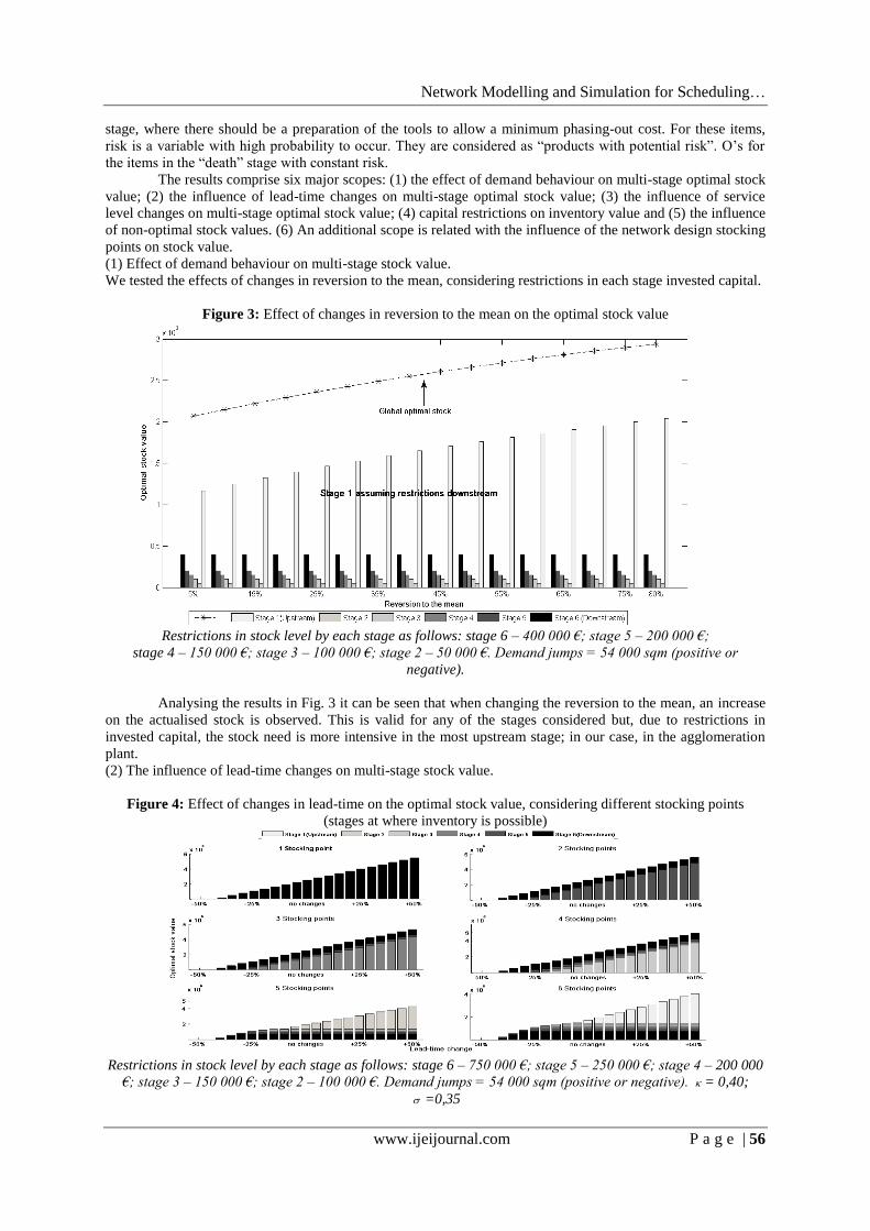
(1) Effect of demand behaviour on multi-stage stock value.

We tested the effects of changes in reversion to the mean, considering restrictions in each stage invested capital.

Figure 3: Effect of changes in reversion to the mean on the optimal stock value

Restrictions in stock level by each stage as follows: stage 6 – 400 000 €; stage 5 – 200 000 €;

stage 4 – 150 000 €; stage 3 – 100 000 €; stage 2 – 50 000 €. Demand jumps = 54 000 sqm (positive or

negative).

Analysing the results in Fig. 3 it can be seen that when changing the reversion to the mean, an increase

on the actualised stock is observed. This is valid for any of the stages considered but, due to restrictions in

invested capital, the stock need is more intensive in the most upstream stage; in our case, in the agglomeration

plant.

(2) The influence of lead-time changes on multi-stage stock value.

Figure 4: Effect of changes in lead-time on the optimal stock value, considering different stocking points

(stages at where inventory is possible)

Restrictions in stock level by each stage as follows: stage 6 – 750 000 €; stage 5 – 250 000 €; stage 4 – 200 000

€; stage 3 – 150 000 €; stage 2 – 100 000 €. Demand jumps = 54 000 sqm (positive or negative). = 0,40;

=0,35



As it can be observed in Fig. 4, that the lead-time reduction, caused by a probable efficiency increase,

results in stock decrease. This is partially explained by the increment of rotation in the planning time frame.

Increases in lead-time originate higher stock needs. As the network is composed by more available stocking

points, the stock tends to decrease, which is consistence with the decrease in the upstream stages’ costs.

(3) The influence of service level changes on multi-stage stock value.

Figure 5: Effect of changes in service level on the optimal stock value, considering different stocking points

(stages at where inventory is possible)

Restrictions in stock level by each stage as follows: stage 6 – 750 000 €; stage 5 – 250 000 €; stage 4 – 200 000

€; stage 3 – 150 000 €; stage 2 – 100 000 €. Demand jumps = 54 000 sqm (positive or negative). = 0,40;

=0,35

Accordingly to the results observed in the former Fig., the optimal stock value is more sensitive to

changes in service level when there is only one possible stocking point. This is essentially explained by the

increase in risks. Thus, it was considered interesting to analyse the impact on the stock value caused by changes

in the service level but also in the number of stocking points, whereas they are downstream or upstream the

supply chain. As simulations where done on the number of stocking points it appears to be clear the

concentration of stocks in the upstream stages of the chain, where the incorporated costs are lower.

(4) Effects of capital restrictions on optimal stock value.

Figure 6: Effect of restrictions in five stages

Demand jumps = 54 000 sqm (positive or negative). = 0,40; =0,35



Figure 7: Effect of restrictions in four stages (no optimal stock in stage 6).


Figure 8: Effect of restrictions in three stages (no optimal stock in stage 5 and 6)


Figure 9: Effect of restrictions in two stages (no stock in stage 4, 5 and 6)




Figure 10: Effect of restrictions in one stages (the only place to put optimal stock is on the stage 1 - upstream)


As it can be notice in Fig. 6 to 10, restrictions affect the optimal stock value. Restrictions affect the

calculation of the optimal value as we impose maximum stocks, which can be different (less) than the optimal

stock according the model to that stage. It is also relevant to emphasize that the concentration of stocks in

upstream stages (intermediate stocks on the plants) tends to decrease the inventory value. The interpretation of

these results can be linked with the concept of premium as it is considered in real options theory. The optimal

stock can be considered an asset that will result in future sales; thus, the value of such asset depends on the time

required to transform stocks into effective sales. In this line of thinking a higher time flow decreases the

premium value, in our case, the optimal stock value. On the other hand we can use the cost and risk theory to

justify that stocks in upstream stages are less risky and less costly (low incorporation of resources).

(5) The influence of non-optimal stock values.

Figure 11: Effect of non-optimal values in different supply chain stages


Fig. 11 presents different scenarios for non-optimal stock values that can result from unbalanced supply

chains, which is normally consequence of the absence of a single authority or to the lack of available

information within the chain partners. We simulated non-optimal values for each stage that is replaced by a

fixed amount of 100 000 € in the following computation in the immediately upstream stage. Non-optimal values

or distortions on the supply chain have a more significant effect on the downstream stages. Fig. 11 shows the

effect on the upstream stage of a non-balanced value. Despite our conceptualisation about a balanced and

integrated supply chain, where decisions are done under a single authority and all the information is available,

there are different realities. From empirical knowledge, the communication distortion is higher as the distance

from the market is amplified. A practical consequence relies on wrong upstream decisions. Based on the results,

we support integration and alignment in inventories decision process to protect the supply chain from the market

uncertainty.



Table (1): Comparison between different strategies

Traditional Approach

Strategy Agile Supply Chain Strategy Multi-stage Scheduling Strategy

1-Stock is held at multiple

echelons.

1-Stock is held at the fewest

echelons.

1-Optimal stock is held at multiple

echelons. The intensity in each

node is related with demand

volatility penetration.

2-Replenishment is driven

sequentially by transfers

from one stocking echelon to

another.

2-Replenishment of all echelons is

driven from actual sales/usage data

collected at the customer interface.

2-Inventory for upstream stages are

dependent of the last downstream

stage stock value.

3-Production is planned by

discrete organizational units

with batch feeds between

discrete systems.

3-Production is planned across

functional boundaries from vendor

to customer, through highly

integrated systems, with minimum

lead times

3-Production is planned across

functional boundaries from

customer to vendor, through highly

integrated systems, according to the

downstream stock level.

4-Majority of stock is fully

finished goods, dispersed

geographically, waiting to be

sold.

4-Majority of stock is held as

"work in progress" awaiting build

instructions.

4-High upstream stocks implies for

a smaller global stock value.

Considering the results and analysing Table 1, there are two main opposite strategies that need to be

balanced. One is to hold the stocks in the upstream stages of the chain, where the adding value to raw material is

small. The main advantages supporting this idea are the minimization of invested capital value and also

additional flexibility, due to the possibility of redirecting a common semi-finished item into different finished

items, according to market needs. The other strategy is having a faster service by holding the inventory closer to

the market, in order to improve the service level. This idea can have negative impacts on additional invested

capital value and on the stock risk, due to a higher number of items.

VI. CONCLUSIONS In this paper we have presented a model that focus on distribution network stock optimization

considering capacity restrictions, number of stocking points, value restrictions and non-optimal values impact.

The contribution of this paper is to provide a new modelling framework for supply chain network scheduling

issues and to study how capacity, value, integration management and design restrictions cope with stochastic

demand. Accordingly, we simulated changes impact on a distribution network design problem. The results

demonstrate the importance of flexible distribution networks and integrated communication and management

practices.

This research focused on supply chain network issues in the context of global trade. Several scenarios

were considered based on various network configurations and restrictions. This model provides a tool for the

logistic decision makers, enabling them to optimize decisions related to scheduling problems while integrating

issues of market uncertainty and net resources restrictions impact. At the end we promote an interdisciplinary

model where logistic decisions coop with management financial tools.

We believe that models such as this can play a particularly important role in guiding the overall operations of

target-scale manufacturing and distribution networks at longer-term planning levels. We believe that the

implementation of global profit maximization models represents a potentially significant unrealized opportunity

worthy of serious consideration by many firms.

REFERENCES 1) Ahiska, S.; King, R.. Inventory policy characterizations over the life cycle of a remanufacturable

product. Proceedings of IIE Annual Conference, Norcross, 2009, 1280-1285.

2) Akerkar, R. A.; Lingras, P. An Intelligent Web: Theory and Practice, 1st edn. 2008, Johns and Bartlett,

Boston.

3) Albert, R.; Jeong, H.; Barabási, A.-L. Diameter of the world-wide Web. Nature, 1999, 401, pp. 130–

131.

4) Arntzen, B.; Brown, G.; Harrison, T.; Trafton, L.. Global supply chain management at digital

equipment corporation, Interfaces, 1995, 25, 1, 69-93.

5) Ballou, R.H.. Business Logistics Management. 4th edition. Englewood Cliffs, NJ: Prentice Hall. 1999.



6) Banerjee, A.; Kim, S.; Burton, J.. Supply chain coordination through effective multi-stage inventory

linkages in a JIT environment. International Journal of Production Economics, 2007, 108(1-2), 271-

280.

7) Banker, S.. The tax efficient supply chain, Supply Chain Management Review, 2009, 13, 2, 44-49.

8) Bengtsson, J. Manufacturing flexibility and real options. Department of Production Economics, I IE,

Linköping Institute of Technology, 2001, S-581 83, Linköping, Sweden.

9) Berry M. W., Dumais S. T., O’Brien G. W. Using linear algebra for intelligent information retrieval,

SIAM Review, 1995, 37, pp. 573-595.

10) Bharat, K.; Broder, A. A technique for measuring the relative size and overlap of public Web search

engines. Computer Networks, 1998, 30(1–7), pp. 107–117.

11) Broder, A.; Kumar, R.; Maghoul, F.; Raghavan, P.; Rajagopalan, S.; Stata, R.; Tomkins, A.; Wiener, J.

Graph structure in the Web. Computer Networks, 2000, 33(1–6), pp. 309–320.

12) Chakrabarti, S. Data mining for hypertext: A tutorial survey. SIGKDD explorations, 2000, 1(2), pp. 1–

11.

13) Chan, F.T.; Chan, H.K.. Effects of cascade information sharing in inventory and service level in multi-

echelon supply chains. International Journal of Business Performance and Supply Chain Modelling,

2009, 1(1), 1-7.

14) Chen, F.. Decentralized supply chains subject to information delays. Management Science, 1999, 45,

1076-1090.

15) Creazza, A.; Dallari, F., Melacini, M.. Evaluating logistics network configurations for a global supply

chain, Supply Chain Management, 2010, 15, 2, 154-164.

16) Cutting-Decelle A-F.; Young B. I.; Das B.P.; Case K.; Rahimifard S.; Anumba C.J.; Bouchlaghem

D.M. A review of approaches to supply chain communications: from manufacturing to construction,

ITcon, 2007, 12, 73-102.

17) Daley, M.. Exploring the relationship between supply network configuration, inter-organizational

information sharing and performance, Managerial Sciences Dissertations. 2008, Paper 16.

18) Daskin, M.; Coullard, C.. An inventory-location model: Formulation, solution algorithm and

computational results, Annals of Operations Research, 2002, 110, 1, 83-83.

19) Dong, J.; Zhang, D.; Hong, Y.; Nagurney, A.. Multitiered Supply Chain Networks: Multicriteria

Decision-Making Under Uncertainty, Annals of Operations Research, 2005, 135, 1, 155-178.

20) Forslund, H.; Jonsson, P.. The impact of forecast information quality on supply chain performance.

International Journal of Operations & Production Management, 2007, 27(1), 90-107.

21) Garavelli, A.. Flexibility configurations for the supply chain management, International Journal of

Production Economics, 2003, 85, 2, 141-153.

22) Graves, S.; Willems, S.. Optimizing the supply chain configuration for new products, Working Paper.

Leaders for Management Program and A.P. Sloan School of Management, MIT, 2001.

23) Guillén, G.; Mele, F.; Bagajewicz, M.; Espuna, A.; Puigjaner, L.. Multiobjective supply chain design

under uncertainty, Chemical Engineering Science, 2005, 60, 6, 1535-1553.

24) Hsu, V.; Zhu, K.. Tax-Effective Supply Chain Decisions under China's Export-Oriented Tax Policies,

Manufacturing and Service Operations Management, 2011, 13, 2, 163-179.

25) Hume, K.. Building a better supply chain, Frontline Solutions, 2003, 4, 11, 16-18.

26) Irving, D.; Kilponen, R.; Markarian, G.; Klitgaard, M.. A tax-aligned approach to SCM, Supply Chain

Management Review, 2005, 9, 3, 57-61.

27) Lambert, D.; Cooper, M.; Pagh, J.. Supply chain management: more than a name for logistics,

International Journal of Logistics Management, 1997, 8, 1, 1-14.

28) Lee, H.; Padmanabhan, V.; Whang, S.. Information Distortion in a Supply Chain: The Bullwhip Effect,

Management Science, 1997, 43, 4, 546-558.

29) Leger, P.; Cassivi, L.; Hadaya, P.; Caya, O.. Safeguarding Mechanisms in a Supply Chain Network,

Industrial Management and Data Systems, 2006, 106, 6, 759-777.

30) Li, X.. Optimal inventory policies in decentralized supply chains. International Journal of Production

Economics, 2010, 128(1), 303-309.

31) Liu, B.; Berger, P.; Zeng, A.; Gerstenfeld, A.. Applying the analytic hierarchy process to the offshore

outsourcing location decision, Supply Chain Management: An International Journal, 2008, 13, 6, 435-

49.

32) Liu, S., Young, I.M.; Ding, L.. An integrated decision support system for global manufacturing co-

ordination in the automotive industry. International Journal of Computer Integrated Manufacturing,

2011, 24(4), 285-301.

33) Lovell, A.; Saw, R.; Stimson, J.. Product value density: managing diversity through supply chain

segmentation, The International Journal of Logistics Management, 2005, 16, 1, 142-58.



34) Ma, H.; Davidrajuh, R.. An Iterative Approach for Distribution Chain Design in Agile Virtual

Environment, Industrial Management and Data System, 2005, 105, 6, 815-834.

35) Mangal, D.; Chandna, P.. Inventory Control in Supply Chain Through Lateral Transshipment – A Case

Study. In Indian Industry. International Journal of Engineering, 2009, 3(5), 443-457.

36) Moser, R.; Kern, D.; Wohlfarth, S.; Hartmann, E.. Supply network configuration benchmarking,

Benchmarking, 2011, 18, 6, 783-801.

37) Nagurney, A.; Dong, J.; Zhang, D.. A Supply Chain Network Equilibrium Model”, Transportation

Research, 2002, 38, E, 281–303.

38) Oster, L.. How to benefit when the supply chain meets tax, Supply Chain Brain, 2009, 18, available at:

www.supplychainbrain.com.

39) Petersen, K.; Ragatz, G., Monczka, R.. An examination of collaborative planning effectiveness and

supply chain performance. The Journal of Supply Chain Management, 2005, 41(2), 14-25.

40) Samaddar, S.; Nargundkar, S.; Daley, M.. Inter-organizational information sharing: The role of supply

network configuration and partner goal congruence, European Journal of Operational Research, 2006,

174, 2, 744-65.

41) Srai, J.; Gregory, M.. A supply network configuration perspective on international supply chain

development, International Journal of Operations and Production Management, 2008, 28, 5, 386-411.

42) Tan, B.. Managing manufacturing risks by using capacity options. Journal of the Operational Research

Society, 2002, 53, 232-242.

43) Tan, T.. Using Imperfect Advance Demand Information in Forecasting. Department of Technology

Management, Eindhoven University of Technology, IMA Journal of Management Mathematics

Advance, 2008, February 16.

44) Tannous, G.F.. Capital Budgeting for Volume Flexible Equipment. Decision Sciences, 1996, 27(2),

157-184.

45) Tsiakis, P.; Shah, N.; Pantelides, C.. Design of Multi-Echelon Supply Chain Networks Under Demand

Uncertainty, Industrial and Engineering Chemistry Research, 2001, 40, 16, 3585-3604.

46) Wiersema, W. H.. Conquering the inventory problem. Electrical Apparatus, 2008, 61, 1, 32-33.

47) Zeng, Z.; Rossetti, C.. Developing a framework for evaluating the logistics costs in global sourcing

processes: an implementation and insights, International Journal of Physical Distribution and Logistics

Management, 2003, 33, 9, 785-803.

48) Zhang, G.; Saboonchi, B.. Configuring Multi-Stage Global Supply Chains with Uncertain Demand,

Supply Chain Theory and Applications. I-Tech Education and Publishing, 2008, 135-154.

Date post:	13-Mar-2018
Category:	Documents
Upload:	truongduong
View:	222 times
Download:	0 times

Network Modelling and Simulation for Scheduling · PDF fileNetwork Modelling and Simulation...

Documents