NETWORK MODELS FOR CAPTURING MOLECULAR FEATURE AND PREDICTING DRUG TARGET FOR VARIOUS CANCERS Enze Liu Submitted to the faculty of the University Graduate School in partial fulfillment of the requirements for the degree Doctor of Philosophy in the School of Informatics and Computing, Indiana University December 2020
Transcript
NETWORK MODELS FOR CAPTURING MOLECULAR FEATURE AND
PREDICTING DRUG TARGET FOR VARIOUS CANCERS
Enze Liu
Submitted to the faculty of the University Graduate School in partial fulfillment of the requirements
for the degree Doctor of Philosophy
in the School of Informatics and Computing, Indiana University
December 2020
ii
Accepted by the Graduate Faculty of Indiana University, in partial fulfillment of the requirements for the degree of Doctor of Philosophy.
I would like to express my most sincere appreciation to my advisor Professor
Lang Li. Without his guidance, none of these studies can be conducted, not to mention
the PhD thesis work. His great mentorship and rigorous attitude towards scientific
research have forged me. I also would like to send my gratitude to my committee
members: Professor Huanmei Wu, Professor Xiaowen Liu, Professor Chi Zhang,
Professor Jun Wan and Professor Sha Cao. Their comments and suggestions are
priceless. I also would like to thank the School of Informatics and Computing in Indiana
University for their tremendous effect on designing the courses and providing
assistance for all students.
I also would like to thank my colleagues, Dr. Lei Wang, Dr. Xue Wu, Dr.
Pengyue Zhang, Dr. Hen-yi Wu, Mr. Yang Huo, Mr. Chuanpeng Dong. It has been very
educating and fun to collaborate with you.
My appreciation also goes to my parents: Guoming Liu and Jiajia Li, and all my
relatives and friends, for their undoubtable support. Last but not the least, I would like
to thank my fiancée Shijun Zhang. Thank you for being by my side.
iv
Enze Liu
NETWORK MODELS FOR CAPTURING MOLECULAR FEATURE AND
PREDICTING DRUG TARGET FOR VARIOUS CANCERS
Network-based modeling and analysis have been widely used for capturing
molecular trajectories of cellular processes. For complex diseases like cancers, if we
can utilize network models to capture adequate features, we can gain a better insight
of the mechanism of cancers, which will further facilitate the identification of molecular
vulnerabilities and the development targeted therapy. Based on this rationale, we
conducted the following four studies:
A novel algorithm ‘FFBN’ is developed for reconstructing directional regulatory
networks (DEGs) from tissue expression data to identify molecular features. ‘FFBN’
shows unique capability of fast and accurately reconstructing genome-wide DEGs
compared to existing methods. FFBN is further used to capture molecular features
among liver metastasis, primary liver cancers and primary colon cancers.
Comparisons among these features lead to new understandings of how liver
metastasis is similar to its primary and distant cancers.
‘SCN’ is a novel algorithm that incorporates multiple types of omics data to
reconstruct functional networks for not only revealing molecular vulnerabilities but also
predicting drug targets on top of that. The molecular vulnerabilities are discovered via
tissue-specific networks and drug targets are predicted via cell-line specific networks.
SCN is tested on primary pancreatic cancers and the predictions coincide with current
treatment plans.
v
‘SCN website’ is a web application of ‘SCN’ algorithm. It allows users to easily
submit their own data and get predictions online. Meanwhile the predictions are
displayed along with network graphs and survival curves.
‘DSCN’ is a novel algorithm derived from ‘SCN’. Instead of predicting single
targets like ‘SCN’, ‘DSCN’ applies a novel approach for predicting target combinations
using multiple omics data and network models.
In conclusion, our studies revealed how genes regulate each other in the form
of networks and how these networks can be used for unveiling cancer-related
biological processes. Our algorithms and website facilitate capturing molecular
features for cancers and predicting novel drug targets.
Xiaowen Liu, PhD, Co-Chair
Huanmei Wu, PhD, Co-Chair
vi
TABLE OF CONTENTS
List of Tables ........................................................................................................... viii List of Figures ........................................................................................................... ix 1. Introduction ........................................................................................................ 1 2. Background ........................................................................................................ 4
2.3 Model evaluation and Validations ................................................................... 13 2.4 Drug targets discovery ................................................................................... 15
3. A fast and Furious Bayesian Network (FFBN) and Its Application to Identify Colon Cancer to Liver Metastasis Molecular Features ............................................. 18
3.1 Introduction .................................................................................................... 18 3.2 Materials and Methods ................................................................................... 19
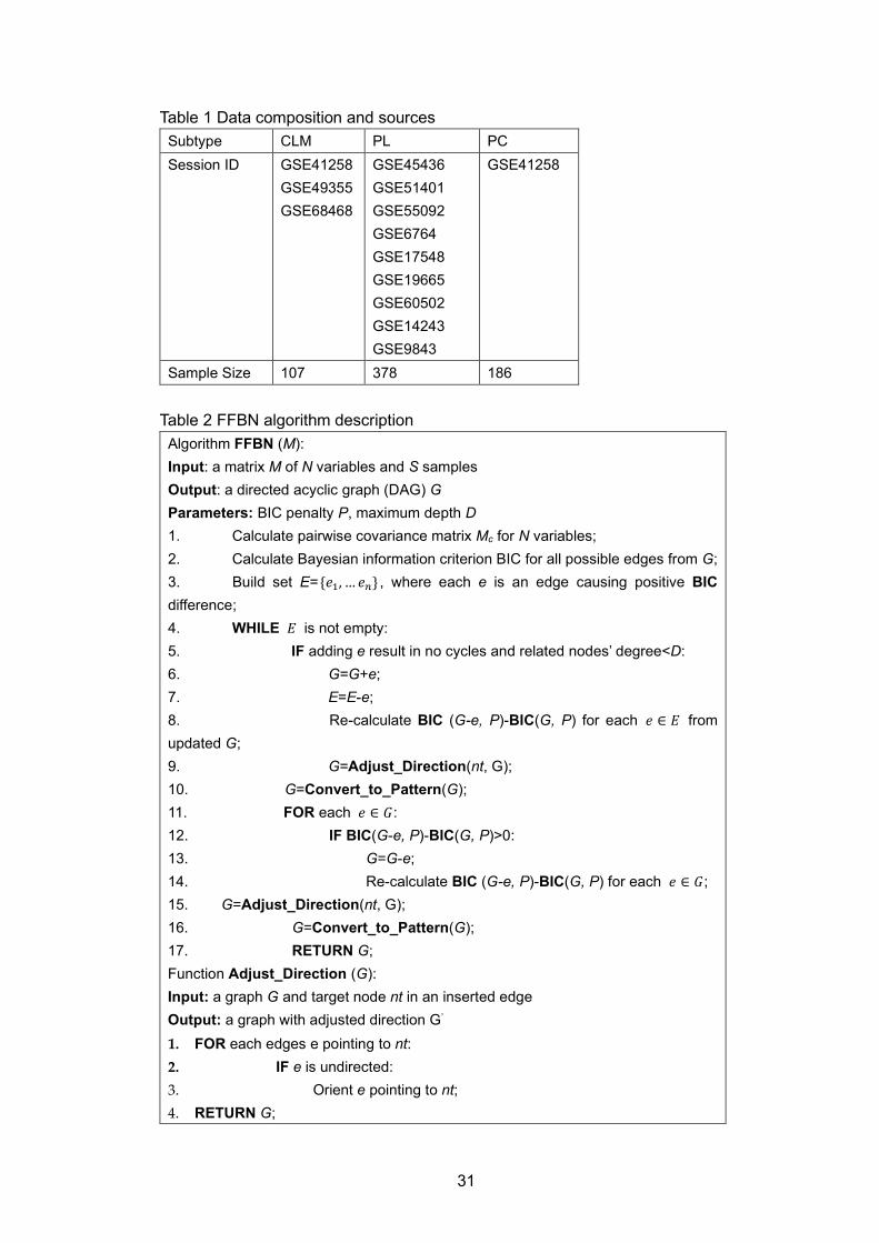
3.2.1 Data availability ....................................................................................... 19 3.2.2 FFBN algorithm ....................................................................................... 20
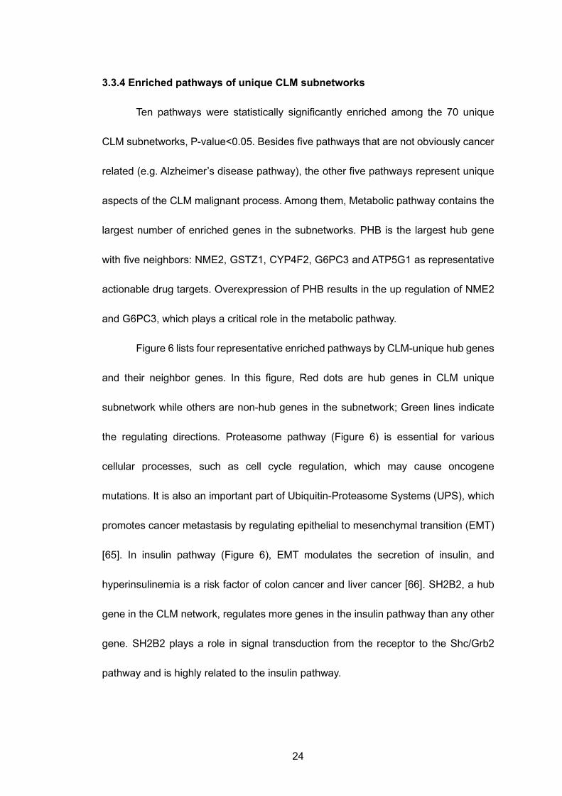
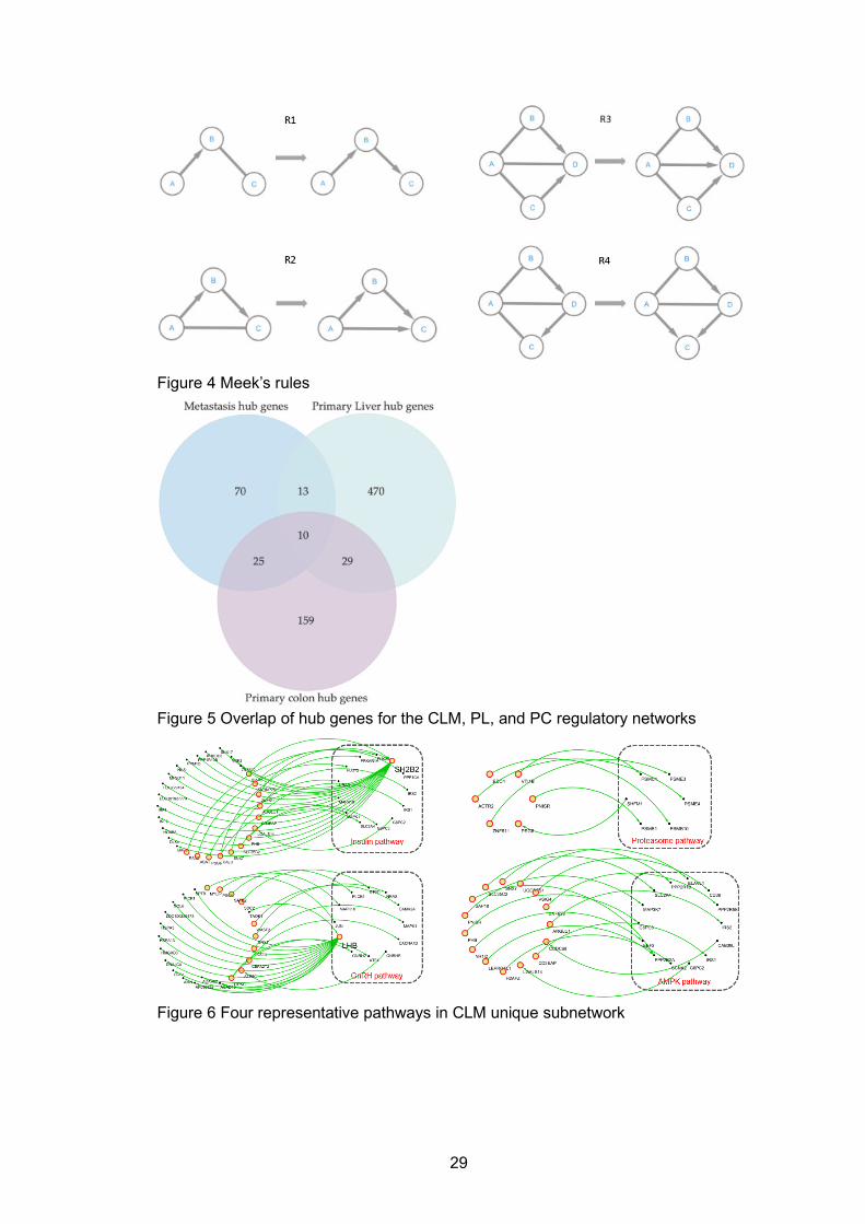
3.3 Results ........................................................................................................... 21 3.3.1 Benchmark results ................................................................................... 21 3.3.2 Constructing GRNs for liver cancer, colon cancer and colon to liver metastasis using FFBN on a whole transcriptome scale ................................... 22 3.3.3. Hub genes matching with oncoKB and Functional comparisons among subnetworks of CLM, PL and PC via pathways ..................................... 23 3.3.4 Enriched pathways of unique CLM subnetworks ...................................... 24 3.3.5 Enriched pathways of CLM-PC common subnetworks ............................. 25 3.3.6 Enriched pathways of CLM-PL common subnetworks ............................. 26
3.4 Discussion ..................................................................................................... 27 4. SCN: Spectral Clustering for Network Based Ranking to Reveal Potential Drug Targets and Its Application in Pancreatic Ductal Adenocarcinoma .................. 34
4.1 Introduction ............................................................................................... 34 4.2 Materials and Methods ................................................................................... 36
4.3 Results ........................................................................................................... 42 4.3.1 Potential target subnetworks and targets for PDAC by SCN algorithm identification ..................................................................................................... 42 4.3.2 Pathway enrichment analysis for top three ranked targets and their clusters ............................................................................................................. 45 4.3.3 Target selection validation by clinical outcomes ....................................... 46
vii
4.3.4 Targets accordance comparison between clinical drug treatment in pancreatic cancer and selection by SCN algorithm ........................................... 46
4.4 Discussion ..................................................................................................... 47 5. SCN Website: Graphical Computation for Prioritization of Cancer Therapeutic Targets Using CRISPR–Cas9 Screen ..................................................................... 52
5.1 Introduction .................................................................................................... 52 5.2 Materials and Methods ................................................................................... 53
6. D-SCN: A Spectral Clustering based Network approaches for Double drug- Targets Prioritization for Cancers ............................................................................ 59
6.1 Introduction .................................................................................................... 59 6.2 Materials and Methods ................................................................................... 62
6.3 Results ........................................................................................................... 73 6.3.1 Routing method selection ........................................................................ 73 6.3.2 Benchmark between DSCN, VIPER and Opticon .................................... 74 6.3.3 Top ranked drug combinations and associated subnetworks ................... 75 6.3.4 Comparison between predictions of DSCNi and existing drug synergies in cell-lines. ...................................................................................................... 76
6.4 Discussion ..................................................................................................... 79 7. Conclusion and Future Work ............................................................................... 89
7.1 Conclusion on FFBN algorithm (section 3) ..................................................... 89 7.2 Conclusion on SCN algorithm (section 4) ....................................................... 89 7.3 Conclusion on SCN website (section 5) ......................................................... 91 7.4 Conclusion on DSCN algorithm (section 6) .................................................... 91
References .............................................................................................................. 93 Curriculum Vitae
viii
LIST OF TABLES
Table 1 Data composition and sources .................................................................... 31 Table 2 FFBN algorithm description ......................................................................... 31 Table 3 Benchmark results of FFBN and FGS ......................................................... 32 Table 4 Summary of three generated GRNs ............................................................ 33 Table 5 Gene expression data used in ‘SCN’ study ................................................. 51 Table 6 The top 12 ranked drug targets and associated gene expression
variation in tumors ........................................................................................ 51 Table 7 Compositions and sources of pancreatic omics-data ................................... 86 Table 8 Spearman correlations between predicted target combinations and
documented SL pairs .................................................................................... 86 Table 9 Top ranked target combinations and their statistics ..................................... 87 Table 10 Contingency table of predicted synergy and actual drug synergy .............. 87 Table 11 Top ranked and selected target combinations and corresponding drug
combinations from DSCNi ............................................................................ 88
ix
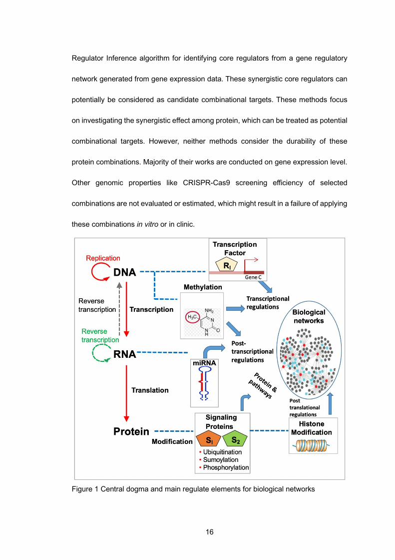
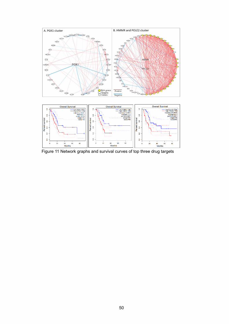
LIST OF FIGURES Figure 1 Central dogma and main regulate elements for biological networks .......... 16 Figure 2 Central dogma and corresponding networks at each level ......................... 17 Figure 3 Representative models for reconstructing regulatory network .................... 17 Figure 4 Meek’s rules .............................................................................................. 29 Figure 5 Overlap of hub genes for the CLM, PL, and PC regulatory networks ......... 29 Figure 6 Four representative pathways in CLM unique subnetwork ......................... 29 Figure 7 Regulations among genes involved in the T cell response pathway ........... 30 Figure 8 Regulations among genes in oxidative phosphorylation pathway .............. 30 Figure 9 Workflow of ‘SCN ...................................................................................... 49 Figure 10 Heatmap of PGK1 and POLE2-HMMR clusters in three groups .............. 49 Figure 11 Network graphs and survival curves of top three drug targets .................. 50 Figure 12 Website Structures of data processing, output type and visualization ...... 57 Figure 13 Example outputs of SCN website ............................................................ 58 Figure 14 Three different routing methods ............................................................... 82 Figure 15 DSCN and DSCNi workflow ..................................................................... 82 Figure 16 Score difference under different routing methods .................................... 83 Figure 17 Subnetwork No.42 in tissue specific network ........................................... 84 Figure 18 Subnetwork No.42 in cell-line specific network ........................................ 85
1
1 Introduction
Modern system biology focuses on understanding how genes and other
molecules work in concert as a complex system to form and regulate biological
processes in every living organism [1]. These regulations consist of various types: Cis-
regulatory elements and trans-regulatory elements are two main regulatory types [2].
Cis-regulatory elements are present near the structural portion of the gene/protein as
the gene they regulate, such as the photosynthetic protein family, are expressed at the
same time in development. Whereas trans-regulatory elements can distantly regulate
genes from which they were transcribed. Enhancers and multiple trans-acting factors
are essential for trans-control transcription initiations. Regulators contain DNA
epigenetic modifications by methylation, miRNA, transcription factors (TFs), and post-
translational modification (PTM) that include histone proteins and other proteins, which
are involved in methylation, phosphorylation, acetylation, ubiquitylation, and
sumoylation (Figure 1). A motif is a sequence pattern that carries out certain functions
in DNA, RNA and proteins. Normally, TFs coded by a gene can regulate gene
expression by binding to specific motifs. MicroRNAs (miRNAs) regulate gene
expression via RNA silencing or post-transcription regulations. Histones can alter the
chromatin structure, which further controls the access of TFs and polymerases to
genes thus resulting in an expression regulation [3]. Methylation plays a crucial role in
regulating gene expression by blocking the promoters that can activate TFs [4]. Large
experimental evidence has been gathered to verify biology gene interactions, such as
Algorithm FFBN (M): Input: a matrix M of N variables and S samples Output: a directed acyclic graph (DAG) G Parameters: BIC penalty P, maximum depth D 1. Calculate pairwise covariance matrix Mc for N variables; 2. Calculate Bayesian information criterion BIC for all possible edges from G; 3. Build set E={𝑒𝑒1, … 𝑒𝑒𝑛𝑛} , where each e is an edge causing positive BIC difference; 4. WHILE 𝐸𝐸 is not empty: 5. IF adding e result in no cycles and related nodes’ degree<D: 6. G=G+e; 7. E=E-e; 8. Re-calculate BIC (G-e, P)-BIC(G, P) for each 𝑒𝑒 ∈ 𝐸𝐸 from updated G; 9. G=Adjust_Direction(nt, G); 10. G=Convert_to_Pattern(G); 11. FOR each 𝑒𝑒 ∈ 𝐺𝐺: 12. IF BIC(G-e, P)-BIC(G, P)>0: 13. G=G-e; 14. Re-calculate BIC (G-e, P)-BIC(G, P) for each 𝑒𝑒 ∈ 𝐺𝐺; 15. G=Adjust_Direction(nt, G); 16. G=Convert_to_Pattern(G); 17. RETURN G; Function Adjust_Direction (G): Input: a graph G and target node nt in an inserted edge Output: a graph with adjusted direction G’ 1. FOR each edges e pointing to nt: 2. IF e is undirected: 3. Orient e pointing to nt; 4. RETURN G;
32
Function Convert_to_Pattern (G): Input: a graph G Output: a pattern graph G’
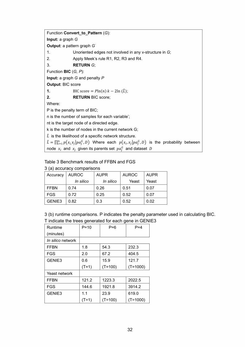
1. Unoriented edges not involved in any v-structure in G; 2. Apply Meek’s rule R1, R2, R3 and R4. 3. RETURN G; Function BIC (G, P): Input: a graph G and penalty P Output: BIC score 1. BIC score = 𝑃𝑃ln(𝑚𝑚) 𝑘𝑘 − 2ln (𝐿𝐿�); 2. RETURN BIC score; Where: P is the penalty term of BIC; n is the number of samples for each variable’; nt is the target node of a directed edge. k is the number of nodes in the current network G; 𝐿𝐿� is the likelihood of a specific network structure. 𝐿𝐿� = ∏ 𝑝𝑝�𝑥𝑥𝑖𝑖,𝑥𝑥𝑗𝑗�𝑝𝑝𝑎𝑎𝑗𝑗𝐺𝐺 ,𝐷𝐷�𝑛𝑛
𝑖𝑖=1 Where each 𝑝𝑝�𝑥𝑥𝑖𝑖 , 𝑥𝑥𝑗𝑗�𝑝𝑝𝑎𝑎𝑗𝑗𝐺𝐺 ,𝐷𝐷� is the probability between node 𝑥𝑥𝑖𝑖 and 𝑥𝑥𝑗𝑗 given its parents set 𝑝𝑝𝑎𝑎𝑗𝑗𝐺𝐺 and dataset 𝐷𝐷
Table 3 Benchmark results of FFBN and FGS 3 (a) accuracy comparisons
reflected in drug synergies, target combinations not reflected in drug synergies
respectively. The phi correlation is defined as:
𝜙𝜙 = �𝜒𝜒2
𝑛𝑛, 𝜙𝜙 𝜖𝜖 [−1,1] (42)
where 𝜒𝜒2 indicates the chi-square statistic. 𝜙𝜙 = ±1 reflects maximum
positive/negative correlations between rows and columns in contingency table.
Predicted synergistic target combinations (PS) has a high positive correlation (0.32)
with target combinations reflected in drug synergies. Notably, no PS & DN
combinations occurs in Table 10, indicating that predictions from DSCNi has very few
false positive rates.
7,069 out of 14,067 discovered target combinations are identified as synergistic
combinations. Top 72 of them ranked by TI score are associated with MAPK3 and
another genes, which further point to ARSENIC TRIOXIDE and another compounds.
This is due to the strong synergistic effect between MAPK3 and many other genes.
MAPK3 is often highly expressed in TNBC due to the activation of Ras/MAPK pathway
(Hazard ratio =1.5, p<0.01). Signals from Ras pathway are transmitted through Raf,
MEK, MAPK1/3 to the nucleus to initiate downstream transcription factors such as
MYC, ETS-1, ETS-2, and ELK-1, which further regulate cell proliferation and survival
[147]. Inhibition of Ras/MAPK pathway has been proven as highly effective in treating
advanced melanoma [148] and preventing/treating TNBC metastasis in vivo [149, 150].
ARSENIC TRIOXIDE (As2O3), which has been successfully applied in treating
hematologic malignancies due to its capability of inducing cell apoptosis, has not been
79
widely applied on treating solid tumors, including TNBC. Recent studies suggest that
inhibiting pathways such TNF, JAK and PI3K-Akt work in concert with As2O3 for better
treating TNBC [151-154]. These findings coincide with the predictions of DSCNi.
Other combinations in Table 11 are selected for their high bliss scores, TI
scores and documented synthetic lethality. Among them LAPATINIB, DOCETAXEL,
PACLITAXEL are the most common chemo drugs for treating TNBC and (PACLITAXEL,
LAPATINIB) combinations are widely prescribed.
6.4 Discussion
DSCN is introduced as a method that uses tissue and cell-line models to
discovery and rank target combinations according to their estimated lethality. With
existing evidence from literature and database, it is demonstrated that:
1. Using known SL pairs and non-SL pairs (random combinations of genes in
these SL pairs) as inputs, DSCN clearly distinguishes two groups by their TI scores.
This is mainly due to the selected routing method has the best capability of
distinguishing two groups over other routing methods.
2. Predictions from DSCN directly overlaps with documented SL pairs while
other methods (VIPER and Option) failed to provide any direct overlaps between their
predictions and documented SL pairs. VIPER and Opticon first predicts master
regulators and then estimate the synergies among them, which limit their searching
space. Two master regulators are not necessarily synergistic even though the
subnetworks they control contain a lot of SL pairs. In contrast, even though DSCN is
designed to predict combinations among targets that are associated with FDA
80
approved drugs, it is capable of predict any gene pairs that have expression value and
essentiality, which broaden the searching space. Any potential SL pairs within the
entire genome can be potentially discovered. Moreover, predictions from DSCN
directly reflect the SL between two genes, which are more direct to understand and
easier to be validated.
3. Predicted ranks from DSCN align with documented SL pairs in terms of SL
intensity, especially for top ranked predictions (top 20, Spearman corr=0.43). This
shows great accuracy of predictions. Predicted ranks also align well with (Spearman
corr=0.34) documented PDAC specific SL pairs, indicating a reasonably good
specificity of the DSCN predictions under context specific scenario.
Additionally, compared to VIPER and Opticon, DSCN requires the least
computational time. VIPER requires ARACNe to pre-compute mutual information
network, which cost roughly 6 days to generate with a whole genome scale. ARACNe
does not have option to run in parallel. Opticon distributes whole task into hundreds of
jobs, each of which requires various hours (from 3 hours to 50 hours) to complete. This
process needs to be performed twice: one for disease-specific networks and one for
null networks. Computational work of DSCN mainly consists of two parts: spectral
clustering and scoring targets in subnetworks. The first part requires 2-5 hours and
second part requires 12-24 hours for examining all possible combinations of all 1,423
targets within the whole genome. The whole process can be even accelerated using
multiple threads as DSCN allows user to flexibly choose the number of threads in
parallel.
81
DSCNi undergoes the similar processes as DSCN to discover and rank target
combinations for individuals. One TNBC sample from TCGA and one TNBC cell-line
sample from CCLE are selected as input to predict target combinations. The
predictions are validated using the following schemes:
1. The predictions are compared with existing drug combination synergies.
Predicted synergistic target combinations has a high positive correlation (0.32) with
target combinations reflected in synergistic drug combinations (bliss>0.12). Moreover,
predictions from DSCNi doesn’t have false positives, which is critical for the predictions
to be applied in clinic.
2. Drug combinations associated with top ranked synergistic target
combinations are either widely used in clinic as treatment plans or frequently reported
as novel treatment plans in literatures. Combinations containing As2O3 are top ranked
because their associated target combinations are in the upstream and downstream
areas of Ras/MAPK pathway, which have been already targeted for successfully
treating hematologic malignancies and melanomas. The findings might benefit the
As2O3 associated combinational therapies to be re-purposed on treating TNBC.
3. For the top ranked target combinations, similarities between tissue
subnetworks with and cell-line subnetworks are measured. Two networks are
reasonably similar in terms of expression patterns and gene-gene correlations. This
also strengthens the fact that As2O3 associated combinational therapies can be re-
purposed.
82
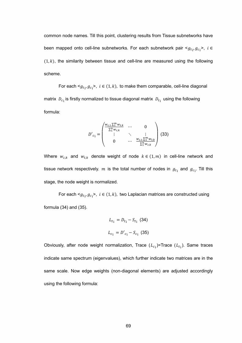
Figure 14 Three different routing methods (a) Original network. The numbers indicate edge weights (b) Heaviest paths between target node 𝑇𝑇1 are all the other nodes (c) Routes constructed by random walk process (d) Hierarchical structures constructed by diffusion process
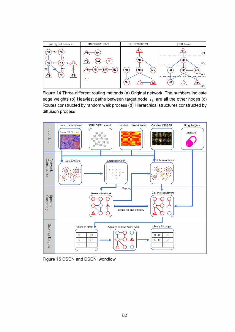
Figure 15 DSCN and DSCNi workflow
83
Figure 16 Score difference under different routing methods
84
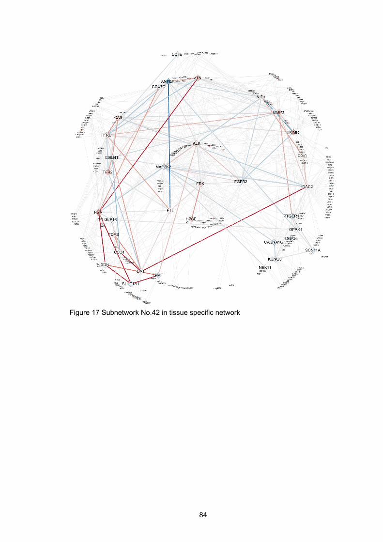
Figure 17 Subnetwork No.42 in tissue specific network
85
Figure 18 Subnetwork No.42 in cell-line specific network
86
Table 7 Compositions and sources of pancreatic omics-data GEO Expression data Perturbation
179 samples 4 samples Table 8 Spearman correlations between predicted target combinations and documented SL pairs
Type Spearman Correlation
P-value SL vs Non-SL
T-statistic P-value
PDAC 0.34 <0.01 PDAC 0.34 <0.01 Top 20 0.43 0.06 Top 20 0.41 0.06 Top 40 0.25 0.11 Top 40 0.24 0.12 Top 100 0.27 0.02 Top 100 0.24 0.01 Total 936 0.16 <0.01 Total 936 0.15 <0.01
87
Table 9 Top ranked target combinations and their statistics Gene1 Gene2 TI score Hazard
The benchmark studies show that GENIE3 has overall best AUROC and AUPR
in silico network, and equally good AUROC but worse AUPR in yeast network
compared to FFBN and FGS. Unlike GENIE3, FFBN infers the GRN purely in a data-
driven way. It doesn’t rely on existing prior knowledge to infer the network structure.
Speed-wise, prior knowledge of TF and no-direction-inferring feature provides GENIE3
the fastest speed among the three methods. FFBN maintains a significantly faster
speed under different parameters and networks with different scales compared to FGS.
The speed increase varies from 11% up to 96%, and the speed difference between
FFBN and FGS becomes larger as the network becomes denser or larger. Taken
together, FFBN shows ascendancy over FGS when reconstructing large and dense
biological networks. This computation advantage is also reflected in the GRN
constructions for CLM, PC, and PL cancer samples. FFBN was able to build up these
GRNs in between 2,430 and 5,931 minutes, while FGS failed to generate a converged
PL GRN, prohibiting any follow-up network comparison and pathway enrichment
analyses.
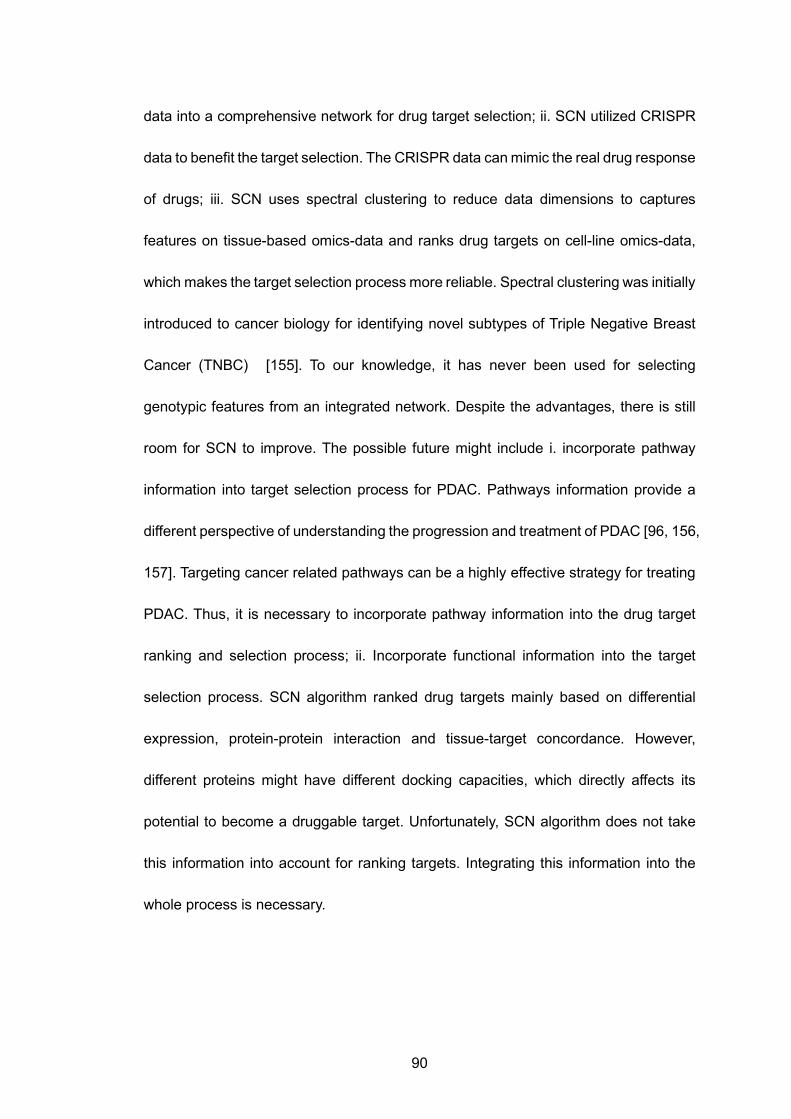
7.2 Conclusion on SCN algorithm (section 4)
SCN is the first algorithm that can incorporate expression data, PPI data and
gene perturbation data (CRISPR or RNAi) for selecting and ranking drug targets. The
novelty of SCN algorithm mainly reflects on: i. SCN is the first algorithm that takes
advantage of dimension reduction methods to integrate three different types of omics
90
data into a comprehensive network for drug target selection; ii. SCN utilized CRISPR
data to benefit the target selection. The CRISPR data can mimic the real drug response
of drugs; iii. SCN uses spectral clustering to reduce data dimensions to captures
features on tissue-based omics-data and ranks drug targets on cell-line omics-data,
which makes the target selection process more reliable. Spectral clustering was initially
introduced to cancer biology for identifying novel subtypes of Triple Negative Breast
Cancer (TNBC) [155]. To our knowledge, it has never been used for selecting
genotypic features from an integrated network. Despite the advantages, there is still
room for SCN to improve. The possible future might include i. incorporate pathway
information into target selection process for PDAC. Pathways information provide a
different perspective of understanding the progression and treatment of PDAC [96, 156,
157]. Targeting cancer related pathways can be a highly effective strategy for treating
PDAC. Thus, it is necessary to incorporate pathway information into the drug target
ranking and selection process; ii. Incorporate functional information into the target
selection process. SCN algorithm ranked drug targets mainly based on differential
expression, protein-protein interaction and tissue-target concordance. However,
different proteins might have different docking capacities, which directly affects its
potential to become a druggable target. Unfortunately, SCN algorithm does not take
this information into account for ranking targets. Integrating this information into the
whole process is necessary.
91
7.3 Conclusion on SCN website (section 5)
SCN website offers a unique method of prioritizing actionable drug targets from
multi-type omics data, including tissue and cell-line expression profiles, PPIs, CRISPR
screening data and drug target information from DrugBank. Over 20,000 genes, 9606
proteins, expression profile from >400 cell-lines across 24 different cancer types are
included. For the first time in precision medicine, this platform integrates tissue data
and cell-line data of cancers, enabling users to upload their own expression data to
seek customized targets. Survival analysis is automatically performed using TCGA
patient data so that users can validate their targets. Moreover, SCN website provides
GSEA analysis for the prioritized targets to better mine the biological mechanisms
associated with them. Additionally, evidence of clinical trials extracted from
ClincalTrials.gov can provide more hints on how the identified targets can be applied
in clinic.
SCN website provides instructions of input, output files and general steps of
SCN algorithm. It offers an complete set of example files, which contains example
tissue expression data, cell-line expression data, all intermediate files generated
during the algorithm processing and example output file so that users can easily
understand and try the whole process.
7.4 Conclusion on DSCN algorithm (section 6)
DSCN and DSCNi has been validated as solid approaches for predicting
lethality for combinational targets. Some of these combinational targets either serve
as widely used in clinic. Other top ranked combinational targets are extensively studied
92
as promising treatment plans. Taken together, these predictions worth further
investigation for either investigating the molecular mechanisms of cancer or
developing novel treatment plans.
93
References
1. Vidal, M.J.F.l., A unifying view of 21st century systems biology. 2009. 583(24): p. 3891-3894.
2. Peters, A., A combination of cis and trans control can solve the hotspot conversion paradox. Genetics, 2008. 178(3): p. 1579-1593.
3. Dong, X. and Z. Weng, The correlation between histone modifications and gene expression. Epigenomics, 2013. 5(2): p. 113-116.
4. Phillips, T., The role of methylation in gene expression. Nature Education, 2008. 1(1): p. 116.
5. Kanehisa, M. and S. Goto, KEGG: kyoto encyclopedia of genes and genomes. Nucleic acids research, 2000. 28(1): p. 27-30.
6. Cerami, E.G., et al., Pathway Commons, a web resource for biological pathway data. Nucleic Acids Res, 2011. 39(Database issue): p. D685-90.
7. Karp, P.D., et al., The metacyc database. Nucleic acids research, 2002. 30(1): p. 59-61.
8. Bryne, J.C., et al., JASPAR, the open access database of transcription factor-binding profiles: new content and tools in the 2008 update. Nucleic acids research, 2007. 36(suppl_1): p. D102-D106.
9. Draizen, E.J., et al., HistoneDB 2.0: a histone database with variants—an integrated resource to explore histones and their variants. Database, 2016. 2016.
10. Cho, S., et al., MiRGator v3. 0: a microRNA portal for deep sequencing, expression profiling and mRNA targeting. Nucleic acids research, 2012. 41(D1): p. D252-D257.
11. Fishilevich, S., et al., GeneHancer: genome-wide integration of enhancers and target genes in GeneCards. Database, 2017. 2017.
12. Cheng, C., et al., Construction and analysis of an integrated regulatory network derived from high-throughput sequencing data. PLoS computational biology, 2011. 7(11).
13. Tong, A.H.Y., et al., Global mapping of the yeast genetic interaction network. 2004. 303(5659): p. 808-813.
14. Margolin, A.A., et al. ARACNE: an algorithm for the reconstruction of gene regulatory networks in a mammalian cellular context. in BMC bioinformatics. 2006. BioMed Central.
15. Stelzl, U., et al., A human protein-protein interaction network: a resource for annotating the proteome. 2005. 122(6): p. 957-968.
16. Venkatesan, K., et al., An empirical framework for binary interactome mapping. Nature methods, 2009. 6(1): p. 83.
17. Baryshnikova, A., et al., Genetic interaction networks: toward an understanding of heritability. Annual review of genomics and human genetics, 2013. 14: p. 111-133.
94
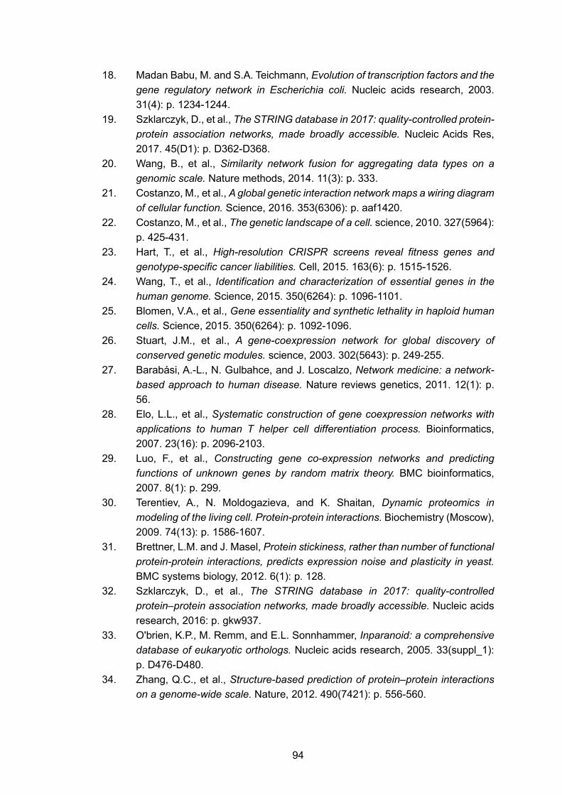
18. Madan Babu, M. and S.A. Teichmann, Evolution of transcription factors and the gene regulatory network in Escherichia coli. Nucleic acids research, 2003. 31(4): p. 1234-1244.
19. Szklarczyk, D., et al., The STRING database in 2017: quality-controlled protein-protein association networks, made broadly accessible. Nucleic Acids Res, 2017. 45(D1): p. D362-D368.
20. Wang, B., et al., Similarity network fusion for aggregating data types on a genomic scale. Nature methods, 2014. 11(3): p. 333.
21. Costanzo, M., et al., A global genetic interaction network maps a wiring diagram of cellular function. Science, 2016. 353(6306): p. aaf1420.
22. Costanzo, M., et al., The genetic landscape of a cell. science, 2010. 327(5964): p. 425-431.
23. Hart, T., et al., High-resolution CRISPR screens reveal fitness genes and genotype-specific cancer liabilities. Cell, 2015. 163(6): p. 1515-1526.
24. Wang, T., et al., Identification and characterization of essential genes in the human genome. Science, 2015. 350(6264): p. 1096-1101.
25. Blomen, V.A., et al., Gene essentiality and synthetic lethality in haploid human cells. Science, 2015. 350(6264): p. 1092-1096.
26. Stuart, J.M., et al., A gene-coexpression network for global discovery of conserved genetic modules. science, 2003. 302(5643): p. 249-255.
27. Barabási, A.-L., N. Gulbahce, and J. Loscalzo, Network medicine: a network-based approach to human disease. Nature reviews genetics, 2011. 12(1): p. 56.
28. Elo, L.L., et al., Systematic construction of gene coexpression networks with applications to human T helper cell differentiation process. Bioinformatics, 2007. 23(16): p. 2096-2103.
29. Luo, F., et al., Constructing gene co-expression networks and predicting functions of unknown genes by random matrix theory. BMC bioinformatics, 2007. 8(1): p. 299.
30. Terentiev, A., N. Moldogazieva, and K. Shaitan, Dynamic proteomics in modeling of the living cell. Protein-protein interactions. Biochemistry (Moscow), 2009. 74(13): p. 1586-1607.
31. Brettner, L.M. and J. Masel, Protein stickiness, rather than number of functional protein-protein interactions, predicts expression noise and plasticity in yeast. BMC systems biology, 2012. 6(1): p. 128.
32. Szklarczyk, D., et al., The STRING database in 2017: quality-controlled protein–protein association networks, made broadly accessible. Nucleic acids research, 2016: p. gkw937.
33. O'brien, K.P., M. Remm, and E.L. Sonnhammer, Inparanoid: a comprehensive database of eukaryotic orthologs. Nucleic acids research, 2005. 33(suppl_1): p. D476-D480.
34. Zhang, Q.C., et al., Structure-based prediction of protein–protein interactions on a genome-wide scale. Nature, 2012. 490(7421): p. 556-560.
95
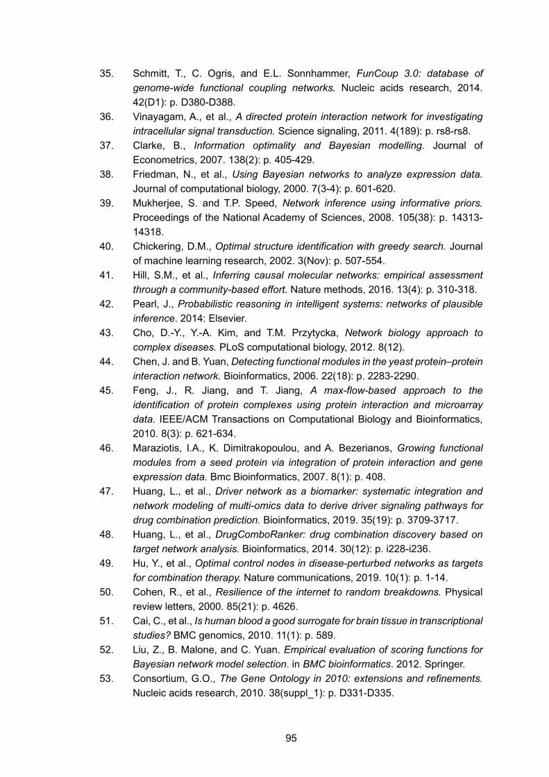
35. Schmitt, T., C. Ogris, and E.L. Sonnhammer, FunCoup 3.0: database of genome-wide functional coupling networks. Nucleic acids research, 2014. 42(D1): p. D380-D388.
36. Vinayagam, A., et al., A directed protein interaction network for investigating intracellular signal transduction. Science signaling, 2011. 4(189): p. rs8-rs8.
37. Clarke, B., Information optimality and Bayesian modelling. Journal of Econometrics, 2007. 138(2): p. 405-429.
38. Friedman, N., et al., Using Bayesian networks to analyze expression data. Journal of computational biology, 2000. 7(3-4): p. 601-620.
39. Mukherjee, S. and T.P. Speed, Network inference using informative priors. Proceedings of the National Academy of Sciences, 2008. 105(38): p. 14313-14318.
40. Chickering, D.M., Optimal structure identification with greedy search. Journal of machine learning research, 2002. 3(Nov): p. 507-554.
41. Hill, S.M., et al., Inferring causal molecular networks: empirical assessment through a community-based effort. Nature methods, 2016. 13(4): p. 310-318.
42. Pearl, J., Probabilistic reasoning in intelligent systems: networks of plausible inference. 2014: Elsevier.
43. Cho, D.-Y., Y.-A. Kim, and T.M. Przytycka, Network biology approach to complex diseases. PLoS computational biology, 2012. 8(12).
44. Chen, J. and B. Yuan, Detecting functional modules in the yeast protein–protein interaction network. Bioinformatics, 2006. 22(18): p. 2283-2290.
45. Feng, J., R. Jiang, and T. Jiang, A max-flow-based approach to the identification of protein complexes using protein interaction and microarray data. IEEE/ACM Transactions on Computational Biology and Bioinformatics, 2010. 8(3): p. 621-634.
46. Maraziotis, I.A., K. Dimitrakopoulou, and A. Bezerianos, Growing functional modules from a seed protein via integration of protein interaction and gene expression data. Bmc Bioinformatics, 2007. 8(1): p. 408.
47. Huang, L., et al., Driver network as a biomarker: systematic integration and network modeling of multi-omics data to derive driver signaling pathways for drug combination prediction. Bioinformatics, 2019. 35(19): p. 3709-3717.
48. Huang, L., et al., DrugComboRanker: drug combination discovery based on target network analysis. Bioinformatics, 2014. 30(12): p. i228-i236.
49. Hu, Y., et al., Optimal control nodes in disease-perturbed networks as targets for combination therapy. Nature communications, 2019. 10(1): p. 1-14.
50. Cohen, R., et al., Resilience of the internet to random breakdowns. Physical review letters, 2000. 85(21): p. 4626.
51. Cai, C., et al., Is human blood a good surrogate for brain tissue in transcriptional studies? BMC genomics, 2010. 11(1): p. 589.
52. Liu, Z., B. Malone, and C. Yuan. Empirical evaluation of scoring functions for Bayesian network model selection. in BMC bioinformatics. 2012. Springer.
53. Consortium, G.O., The Gene Ontology in 2010: extensions and refinements. Nucleic acids research, 2010. 38(suppl_1): p. D331-D335.
96
54. Stark, C., et al., BioGRID: a general repository for interaction datasets. Nucleic acids research, 2006. 34(suppl_1): p. D535-D539.
55. Marbach, D., et al., Wisdom of crowds for robust gene network inference. Nature methods, 2012. 9(8): p. 796.
56. Lamb, J., et al., The Connectivity Map: using gene-expression signatures to connect small molecules, genes, and disease. Science, 2006. 313(5795): p. 1929-35.
57. Ma, Y., et al., Prediction of candidate drugs for treating pancreatic cancer by using a combined approach. PloS one, 2016. 11(2).
58. Alvarez, M.J., et al., Functional characterization of somatic mutations in cancer using network-based inference of protein activity. Nature genetics, 2016. 48(8): p. 838.
59. Ramsey, J.D., Scaling up greedy causal search for continuous variables. arXiv preprint arXiv:1507.07749, 2015.
60. Dennis, G., et al., DAVID: database for annotation, visualization, and integrated discovery. Genome biology, 2003. 4(9): p. R60.
61. Edgar, R., M. Domrachev, and A.E. Lash, Gene Expression Omnibus: NCBI gene expression and hybridization array data repository. Nucleic acids research, 2002. 30(1): p. 207-210.
62. Meek, C., Causal inference and causal explanation with background knowledge. arXiv preprint arXiv:1302.4972, 2013.
63. Irrthum, A., L. Wehenkel, and P. Geurts, Inferring regulatory networks from expression data using tree-based methods. PloS one, 2010. 5(9): p. e12776.
64. Chakravarty, D., et al., OncoKB: a precision oncology knowledge base. JCO precision oncology, 2017. 1: p. 1-16.
65. Voutsadakis, I.A., The ubiquitin–proteasome system and signal transduction pathways regulating epithelial mesenchymal transition of cancer. Journal of biomedical science, 2012. 19(1): p. 67.
66. Giovannucci, E., Insulin and colon cancer. Cancer Causes & Control, 1995. 6(2): p. 164-179.
67. Mihaylova, M.M. and R.J. Shaw, The AMPK signalling pathway coordinates cell growth, autophagy and metabolism. Nature cell biology, 2011. 13(9): p. 1016.
68. Li, W., et al., Targeting AMPK for cancer prevention and treatment. Oncotarget, 2015. 6(10): p. 7365.
69. Vander Heiden, M.G., L.C. Cantley, and C.B. Thompson, Understanding the Warburg effect: the metabolic requirements of cell proliferation. science, 2009. 324(5930): p. 1029-1033.
70. Ashton, T.M., et al., Oxidative phosphorylation as an emerging target in cancer therapy. Clinical Cancer Research, 2018. 24(11): p. 2482-2490.
71. Solaini, G., G. Sgarbi, and A. Baracca, Oxidative phosphorylation in cancer cells. Biochimica et Biophysica Acta (BBA)-Bioenergetics, 2011. 1807(6): p. 534-542.
97
72. Gründker, C. and G. Emons, The role of gonadotropin-releasing hormone in cancer cell proliferation and metastasis. Frontiers in endocrinology, 2017. 8: p. 187.
73. Luo, Y., et al., A network integration approach for drug-target interaction prediction and computational drug repositioning from heterogeneous information. Nat Commun, 2017. 8(1): p. 573.
74. Dimitrakopoulos, C., et al., Network-based integration of multi-omics data for prioritizing cancer genes. Bioinformatics, 2018. 34(14): p. 2441-2448.
75. Ritchie, M.D., et al., Methods of integrating data to uncover genotype-phenotype interactions. Nat Rev Genet, 2015. 16(2): p. 85-97.
76. Kanehisa, M. and S. Goto, KEGG: kyoto encyclopedia of genes and genomes. Nucleic Acids Res, 2000. 28(1): p. 27-30.
77. Nielsen, T.E. and S.L. Schreiber, Towards the optimal screening collection: a synthesis strategy. Angew Chem Int Ed Engl, 2008. 47(1): p. 48-56.
78. Wang, S. and J. Peng, Network-assisted target identification for haploinsufficiency and homozygous profiling screens. PLoS Comput Biol, 2017. 13(6): p. e1005553.
79. Ferrero, E., I. Dunham, and P. Sanseau, In silico prediction of novel therapeutic targets using gene–disease association data. Journal of translational medicine, 2017. 15(1): p. 182.
80. Tsherniak, A., et al., Defining a Cancer Dependency Map. Cell, 2017. 170(3): p. 564-576 e16.
81. Aguirre, A.J., et al., Genomic Copy Number Dictates a Gene-Independent Cell Response to CRISPR/Cas9 Targeting. Cancer Discov, 2016. 6(8): p. 914-29.
82. Cowley, G.S., et al., Parallel genome-scale loss of function screens in 216 cancer cell lines for the identification of context-specific genetic dependencies. Sci Data, 2014. 1: p. 140035.
83. Lin, A., et al., CRISPR/Cas9 mutagenesis invalidates a putative cancer dependency targeted in on-going clinical trials. Elife, 2017. 6: p. e24179.
84. Wei, Y.-C. and C.-K. Cheng. Towards efficient hierarchical designs by ratio cut partitioning. in 1989 IEEE International Conference on Computer-Aided Design. 1989. IEEE.
85. Shi, J. and J. Malik, Normalized cuts and image segmentation. IEEE Transactions on pattern analysis and machine intelligence, 2000. 22(8): p. 888-905.
86. Hartigan, J.A. and M.A. Wong, Algorithm AS 136: A k-means clustering algorithm. Journal of the Royal Statistical Society. Series C (Applied Statistics), 1979. 28(1): p. 100-108.
87. Chiang, M.M.-T. and B. Mirkin, Intelligent choice of the number of clusters in k-means clustering: an experimental study with different cluster spreads. Journal of classification, 2010. 27(1): p. 3-40.
88. Wang, J., et al., A glycolytic mechanism regulating an angiogenic switch in prostate cancer. Cancer Res, 2007. 67(1): p. 149-59.
98
89. Zieker, D., et al., Phosphoglycerate kinase 1 a promoting enzyme for peritoneal dissemination in gastric cancer. Int J Cancer, 2010. 126(6): p. 1513-20.
90. Wang, J., et al., Characterization of phosphoglycerate kinase-1 expression of stromal cells derived from tumor microenvironment in prostate cancer progression. Cancer Res, 2010. 70(2): p. 471-80.
91. Punjabi, P. and A. Murday, Successful surgical repair of a false aneurysm of the ascending aorta following orthotopic cardiac transplantation: a case report. Eur J Cardiothorac Surg, 1997. 11(6): p. 1174-5.
92. Kalmyrzaev, B., et al., Hyaluronan-mediated motility receptor gene single nucleotide polymorphisms and risk of breast cancer. Cancer Epidemiol Biomarkers Prev, 2008. 17(12): p. 3618-20.
93. Shigeishi, H., et al., Overexpression of the receptor for hyaluronan-mediated motility, correlates with expression of microtubule-associated protein in human oral squamous cell carcinomas. Int J Oncol, 2009. 34(6): p. 1565-71.
94. Mootha, V.K., et al., PGC-1alpha-responsive genes involved in oxidative phosphorylation are coordinately downregulated in human diabetes. Nat Genet, 2003. 34(3): p. 267-73.
95. Tang, Z., et al., GEPIA: a web server for cancer and normal gene expression profiling and interactive analyses. Nucleic Acids Res, 2017. 45(W1): p. W98-W102.
96. Cancer Genome Atlas Research, N., et al., The Cancer Genome Atlas Pan-Cancer analysis project. Nat Genet, 2013. 45(10): p. 1113-20.
97. Carithers, L.J., et al., A Novel Approach to High-Quality Postmortem Tissue Procurement: The GTEx Project. Biopreserv Biobank, 2015. 13(5): p. 311-9.
98. Amanam, I. and V. Chung, Targeted Therapies for Pancreatic Cancer. Cancers (Basel), 2018. 10(2).
99. Yamanaka, Y., et al., Overexpression of HER2/neu oncogene in human pancreatic carcinoma. Hum Pathol, 1993. 24(10): p. 1127-34.
100. Chou, A., et al., Clinical and molecular characterization of HER2 amplified-pancreatic cancer. Genome Med, 2013. 5(8): p. 78.
101. Li, X., et al., Mitochondria-Translocated PGK1 Functions as a Protein Kinase to Coordinate Glycolysis and the TCA Cycle in Tumorigenesis. Mol Cell, 2016. 61(5): p. 705-719.
102. Hu, H., et al., Acetylation of PGK1 promotes liver cancer cell proliferation and tumorigenesis. Hepatology, 2017. 65(2): p. 515-528.
103. Xie, H., et al., PGK1 Drives Hepatocellular Carcinoma Metastasis by Enhancing Metabolic Process. Int J Mol Sci, 2017. 18(8).
104. Rajeshkumar, N.V., et al., Therapeutic Targeting of the Warburg Effect in Pancreatic Cancer Relies on an Absence of p53 Function. Cancer Res, 2015. 75(16): p. 3355-64.
105. Grutzmann, R., et al., Gene expression profiling of microdissected pancreatic ductal carcinomas using high-density DNA microarrays. Neoplasia, 2004. 6(5): p. 611-22.
99
106. Tzankov, A., et al., In situ RHAMM protein expression in acute myeloid leukemia blasts suggests poor overall survival. Ann Hematol, 2011. 90(8): p. 901-9.
107. Yamano, Y., et al., Hyaluronan-mediated motility: a target in oral squamous cell carcinoma. Int J Oncol, 2008. 32(5): p. 1001-9.
108. Ishigami, S., et al., Prognostic impact of CD168 expression in gastric cancer. BMC Cancer, 2011. 11: p. 106.
109. Du, Y.C., et al., Receptor for hyaluronan-mediated motility isoform B promotes liver metastasis in a mouse model of multistep tumorigenesis and a tail vein assay for metastasis. Proc Natl Acad Sci U S A, 2011. 108(40): p. 16753-8.
110. Maxwell, C.A., et al., Interplay between BRCA1 and RHAMM regulates epithelial apicobasal polarization and may influence risk of breast cancer. PLoS biology, 2011. 9(11): p. e1001199.
111. Amano, T., et al., Antitumor effects of vaccination with dendritic cells transfected with modified receptor for hyaluronan-mediated motility mRNA in a mouse glioma model. Journal of neurosurgery, 2007. 106(4): p. 638-645.
112. Willemen, Y., et al., The tumor-associated antigen RHAMM (HMMR/CD168) is expressed by monocyte-derived dendritic cells and presented to T cells. Oncotarget, 2016. 7(45): p. 73960-73970.
113. Li, J., X. Ji, and H. Wang, Targeting Long Noncoding RNA HMMR-AS1 Suppresses and Radiosensitizes Glioblastoma. Neoplasia, 2018. 20(5): p. 456-466.
114. Li, J., et al., Knockdown of POLE2 expression suppresses lung adenocarcinoma cell malignant phenotypes in vitro. Oncol Rep, 2018. 40(5): p. 2477-2486.
115. Li, W., et al., MAGeCK enables robust identification of essential genes from genome-scale CRISPR/Cas9 knockout screens. Genome biology, 2014. 15(12): p. 554.
116. Dimitrakopoulos, C., et al., Network-based integration of multi-omics data for prioritizing cancer genes. Bioinformatics, 2018. 34(14): p. 2441-2448.
117. Rauscher, B., et al., GenomeCRISPR-a database for high-throughput CRISPR/Cas9 screens. Nucleic acids research, 2016: p. gkw997.
118. Tsherniak, A., et al., Defining a cancer dependency map. Cell, 2017. 170(3): p. 564-576. e16.
119. Behan, F.M., et al., Prioritization of cancer therapeutic targets using CRISPR–Cas9 screens. Nature, 2019. 568(7753): p. 511.
120. Aguirre, A., et al., Genomic copy number dictates a gene-independent cell response to CRISPR/Cas9 targeting. Cancer Discov. 2016; 6: 914–929. doi: 10.1158/2159-8290. CD-16-0154.[PMC free article][PubMed][Cross Ref].
121. Cowley, G.S., et al., Parallel genome-scale loss of function screens in 216 cancer cell lines for the identification of context-specific genetic dependencies. Scientific data, 2014. 1: p. 140035.
122. Law, V., et al., DrugBank 4.0: shedding new light on drug metabolism. Nucleic acids research, 2013. 42(D1): p. D1091-D1097.
100
123. Tang, Z., et al., GEPIA: a web server for cancer and normal gene expression profiling and interactive analyses. Nucleic acids research, 2017. 45(W1): p. W98-W102.
124. Siegel, R.L., K.D. Miller, and A. Jemal, Cancer statistics, 2019. CA: a cancer journal for clinicians, 2019. 69(1): p. 7-34.
125. Iovanna, J., et al., Current knowledge on pancreatic cancer. Front Oncol, 2012. 2: p. 6.
126. Kruger, S., et al., Translational research in pancreatic ductal adenocarcinoma: current evidence and future concepts. World J Gastroenterol, 2014. 20(31): p. 10769-77.
127. Kamisawa, T., et al., Pancreatic cancer. The Lancet, 2016. 388(10039): p. 73-85.
128. Domenichini, A., et al., Pancreatic cancer tumorspheres are cancer stem-like cells with increased chemoresistance and reduced metabolic potential. Adv Biol Regul, 2019. 72: p. 63-77.
129. Parhi, P., C. Mohanty, and S.K. Sahoo, Nanotechnology-based combinational drug delivery: an emerging approach for cancer therapy. Drug discovery today, 2012. 17(17-18): p. 1044-1052.
130. Gillet, J.-P., S. Varma, and M.M. Gottesman, The clinical relevance of cancer cell lines. Journal of the National Cancer Institute, 2013. 105(7): p. 452-458.
131. Frese, K.K. and D.A. Tuveson, Maximizing mouse cancer models. Nature Reviews Cancer, 2007. 7(9): p. 654.
132. Ran, F.A., et al., Genome engineering using the CRISPR-Cas9 system. Nature protocols, 2013. 8(11): p. 2281-2308.
133. Shi, J., et al., Discovery of cancer drug targets by CRISPR-Cas9 screening of protein domains. Nature biotechnology, 2015. 33(6): p. 661.
134. Wang, T., E.S. Lander, and D.M. Sabatini, Large-Scale Single Guide RNA Library Construction and Use for CRISPR-Cas9-Based Genetic Screens. Cold Spring Harb Protoc, 2016. 2016(3): p. pdb top086892.
135. Vincent, A., et al., Pancreatic cancer. The lancet, 2011. 378(9791): p. 607-620. 136. Liu, Y.-Y., J.-J. Slotine, and A.-L. Barabási, Controllability of complex networks.
nature, 2011. 473(7346): p. 167-173. 137. Sun, Y., et al., Combining genomic and network characteristics for extended
capability in predicting synergistic drugs for cancer. Nature communications, 2015. 6(1): p. 1-10.
138. Barretina, J., et al., The Cancer Cell Line Encyclopedia enables predictive modelling of anticancer drug sensitivity. Nature, 2012. 483(7391): p. 603-607.
139. Wishart, D.S., et al., DrugBank: a comprehensive resource for in silico drug discovery and exploration. Nucleic acids research, 2006. 34(suppl_1): p. D668-D672.
140. Guo, J., H. Liu, and J. Zheng, SynLethDB: synthetic lethality database toward discovery of selective and sensitive anticancer drug targets. Nucleic acids research, 2016. 44(D1): p. D1011-D1017.
101
141. Shoemaker, R.H., The NCI60 human tumour cell line anticancer drug screen. Nature Reviews Cancer, 2006. 6(10): p. 813-823.
142. Margolin, A.A., et al. ARACNE: an algorithm for the reconstruction of gene regulatory networks in a mammalian cellular context. in BMC bioinformatics. 2006. Springer.
143. Jeong, S.M., S. Hwang, and R.H. Seong, Transferrin receptor regulates pancreatic cancer growth by modulating mitochondrial respiration and ROS generation. Biochemical and biophysical research communications, 2016. 471(3): p. 373-379.
144. Xie, Y., et al., Ferroptosis: process and function. Cell Death & Differentiation, 2016. 23(3): p. 369-379.
145. Borisy, A.A., et al., Systematic discovery of multicomponent therapeutics. Proceedings of the National Academy of Sciences, 2003. 100(13): p. 7977-7982.
146. O'Neil, J., et al., An unbiased oncology compound screen to identify novel combination strategies. Molecular cancer therapeutics, 2016. 15(6): p. 1155-1162.
147. Giltnane, J.M. and J.M. Balko, Rationale for targeting the Ras/MAPK pathway in triple-negative breast cancer. Discovery medicine, 2014. 17(95): p. 275-283.
148. Jang, S. and M. Atkins, Treatment of BRAF-mutant melanoma: the role of vemurafenib and other therapies. Clinical Pharmacology & Therapeutics, 2014. 95(1): p. 24-31.
149. Bartholomeusz, C., et al., MEK inhibitor selumetinib (AZD6244; ARRY-142886) prevents lung metastasis in a triple-negative breast cancer xenograft model. Molecular cancer therapeutics, 2015. 14(12): p. 2773-2781.
150. Nagaria, T.S., et al., Combined targeting of Raf and Mek synergistically inhibits tumorigenesis in triple negative breast cancer model systems. Oncotarget, 2017. 8(46): p. 80804.
151. Xin, X., et al., Inhibition of FEN1 Increases Arsenic Trioxide-Induced ROS Accumulation and Cell Death: Novel Therapeutic Potential for Triple Negative Breast Cancer. Frontiers in Oncology, 2020. 10.
152. Alipour, F., et al., Inhibition of PI3K pathway using BKM120 intensified the chemo-sensitivity of breast cancer cells to arsenic trioxide (ATO). The international journal of biochemistry & cell biology, 2019. 116: p. 105615.
153. Pei, X., et al., Effect of tetrandrine combined with arsenic trioxide on stem cells of triple negative breast cancer. 2019.
154. Miodragović, Ð., et al., Beyond cisplatin: Combination therapy with arsenic trioxide. Inorganica Chimica Acta, 2019. 496: p. 119030.
155. Wang, B., et al., Similarity network fusion for aggregating data types on a genomic scale. Nat Methods, 2014. 11(3): p. 333-7.
156. Eser, S., et al., Oncogenic KRAS signalling in pancreatic cancer. British journal of cancer, 2014. 111(5): p. 817.
157. Neuzillet, C., et al., Targeting the TGFβ pathway for cancer therapy. Pharmacology & therapeutics, 2015. 147: p. 22-31.
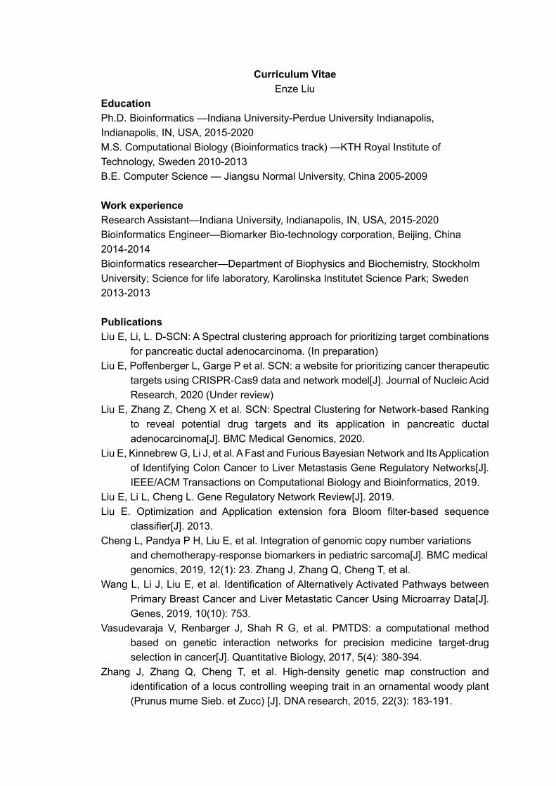
Curriculum Vitae Enze Liu
Education Ph.D. Bioinformatics —Indiana University-Perdue University Indianapolis, Indianapolis, IN, USA, 2015-2020 M.S. Computational Biology (Bioinformatics track) —KTH Royal Institute of Technology, Sweden 2010-2013 B.E. Computer Science — Jiangsu Normal University, China 2005-2009 Work experience Research Assistant—Indiana University, Indianapolis, IN, USA, 2015-2020 Bioinformatics Engineer—Biomarker Bio-technology corporation, Beijing, China 2014-2014 Bioinformatics researcher—Department of Biophysics and Biochemistry, Stockholm University; Science for life laboratory, Karolinska Institutet Science Park; Sweden 2013-2013 Publications Liu E, Li, L. D-SCN: A Spectral clustering approach for prioritizing target combinations
for pancreatic ductal adenocarcinoma. (In preparation) Liu E, Poffenberger L, Garge P et al. SCN: a website for prioritizing cancer therapeutic
targets using CRISPR-Cas9 data and network model[J]. Journal of Nucleic Acid Research, 2020 (Under review)
Liu E, Zhang Z, Cheng X et al. SCN: Spectral Clustering for Network-based Ranking to reveal potential drug targets and its application in pancreatic ductal adenocarcinoma[J]. BMC Medical Genomics, 2020.
Liu E, Kinnebrew G, Li J, et al. A Fast and Furious Bayesian Network and Its Application of Identifying Colon Cancer to Liver Metastasis Gene Regulatory Networks[J]. IEEE/ACM Transactions on Computational Biology and Bioinformatics, 2019.
Liu E, Li L, Cheng L. Gene Regulatory Network Review[J]. 2019. Liu E. Optimization and Application extension fora Bloom filter-based sequence
classifier[J]. 2013. Cheng L, Pandya P H, Liu E, et al. Integration of genomic copy number variations
and chemotherapy-response biomarkers in pediatric sarcoma[J]. BMC medical genomics, 2019, 12(1): 23. Zhang J, Zhang Q, Cheng T, et al.
Wang L, Li J, Liu E, et al. Identification of Alternatively Activated Pathways between Primary Breast Cancer and Liver Metastatic Cancer Using Microarray Data[J]. Genes, 2019, 10(10): 753.
Vasudevaraja V, Renbarger J, Shah R G, et al. PMTDS: a computational method based on genetic interaction networks for precision medicine target-drug selection in cancer[J]. Quantitative Biology, 2017, 5(4): 380-394.
Zhang J, Zhang Q, Cheng T, et al. High-density genetic map construction and identification of a locus controlling weeping trait in an ornamental woody plant (Prunus mume Sieb. et Zucc) [J]. DNA research, 2015, 22(3): 183-191.
Li J, Huo Y, Wu X, et al. Essentiality and Transcriptome-Enriched Pathway Scores Predict Drug-Combination Synergy[J]. Biology, 2020, 9(9): 278.