1

Fabio Martignon

Laboratoire de Recherche en Informatique

Network Optimization

Université Paris Sud

2

Lecture overview

� Multi-commodity flow problem

� Network design problem

– Node positioning

– Users’ coverage (Assignment problem)

– Traffic routing

� Radio/coverage planning

3

Multi-commodity flow problem

4

Multi-commodity flow problem

Given:

An oriented graph G = (N, A).

The capacity uij and the cost cij are associated with each arc (i , j) ∈ A.

A set of demands K, where each demand k is characterized by:

�Source sk ∈ N

�Destination tk ∈ N

�An amount of flow dk

� Problem:

� Route all the demands at the least cost, taking into account the capacity constraints of the arcs.

5

Multi-commodity flow problem (cont.)

6

Model

Decision variables:

The amount of flow (xkij) of demand k routed on arc

(i , j):

Objective function:

7

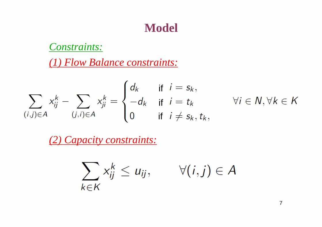
Model

Constraints:

(1) Flow Balance constraints:

(2) Capacity constraints:

if

if

if

8

Model

Constraints:

(3) Positivity constraints:

9

Formulation dimension

� Number of variables: |A||K|

� Number of constraints: |N||K| + |A|

10

Network design problem

11

Candidate SitesTest PointsDestinations

12

Candidate SitesTest PointsDestinations

13

Candidate SitesTest PointsDestinationsRouters

14

Candidate SitesTest PointsDestinationsRouters

15

Network design problemGiven

� A set of Candidate Sites (CSs, where to install nodes)

� A set of test points (TPs) and a set of destinations (DNs)

– source-destination traffic pairs (sk, tk)

Problem

� Install nodes, links, and route traffic demands minimizing the total network installation cost

16

Network modelNotations and parameters:� S: the set of CSs

� I: the set of TPs

� D: the set of DNs

� cIj: cost for installing a node in CS j

� cBjl: cost for buying one bandwidth unit between

CSsj and l

� cAij: Access cost per bandwidth unit between TP i

and CS j

� cEjk: Egress cost per bandwidth unit between CS j

and DN k

17

Notations and parameters:

� dik: traffic generated by TP i towards DN k

� ujl: maximum capacity that can be reserved on link (j,l)

� vj: maximum capacity of the access link of CS j

� hjk: maximum capacity that can be reserved on egress link (j,k)

� aij: 0-1 parameter that indicates if TP i can access the network through CS j

� bjl: 0-1 parameter that indicates if CSj can be connected to CSl

� ejk: 0-1 parameter that indicates if CS j can be connected to DN k

Network model (cont.)

18

Network model (cont.)Decision variables:

� xij: 0-1 variable that indicates if TP i is assigned to CS j

� zj: 0-1 variable that indicates if a node is installed in CS j

� wjk: 0-1 variable that indicates if CSj is connected to DN k

� fkjl: flow variable which denotes the traffic flow

routed on link (j,l) destined to DN k

� fjk: flow variable which denotes the traffic flow routed on egress link(j, k)

19

Network model (cont.)Objective function:The objective function accounts for the total network cost, including installation costs and the costs related to the connection of nodes, users’ access and egress costs.

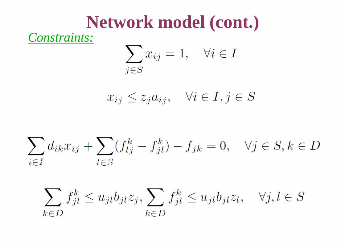
Network model (cont.)Constraints:

21

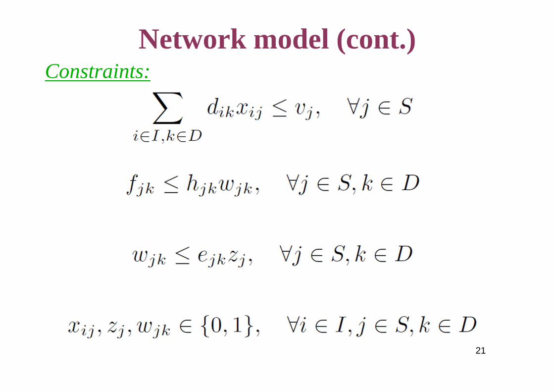
Network model (cont.)Constraints:

22

� AMPL means “A Mathematical Programming Language”

� AMPL is an implementation of the Mathematical Programming language

� Many solvers can work with AMPL

� AMPL works as follows:

� translates a user-defined model to a low-level formulation (called flat form) that can be understood by a solver

� passes the flat form to the solver

� reads a solution back from the solver and interprets it within the higher-level model (called structured form)

AMPL basics

23

� AMPL usually requires three files:

� the model file (extension .mod) holding the MP formulation

� the data file (extension .dat), which lists the values to be assigned to each parameter symbol

� the run file (extension .run), which contains the (imperative) commands necessary to solve the problem

� The model file is written in the MP language

� The data file simply contains numerical data together with the corresponding parameter symbols

� The run file is written in an imperative C-like language (many notable differences from C, however)

� Sometimes, MP language and imperative language commands can be mixed in the same file (usually the run file)

� To run AMPL, type ampl my-runfile.run from the command line

AMPL basics (cont.)

24

costModel.modset D; # set of destinationsset TP; # set of TPsset CS; # set of CSs

param ITP{TP,CS}; # Matrix aij (TP/CS)param ID{CS,D}; # Matrix eij (CS/D)param ICS{CS,CS}; # Matrix bjl (CS/CS)param d{TP,D}; # Traffic generated by each TP, destined to destination Dparam U{CS,CS}; # Capacity on the link CS/CSparam costU{CS,CS}; # Transport cost (per unit of bandwidth) for traffic on the transport link between the CSsparam V{CS}; # Capacity of the link between each TP and CSparam costR{CS}; # Router installation costparam costD{CS,D}; # Cost (per bandwidth unit) for traffic on the link between the CS and the

destination Dparam costTP{TP,CS}; # Cost (per bandwidth unit) for traffic on the link between the TP and the

CSparam H{CS,D}; # Capacity of the egress link CS/D

var x{TP,CS} binary; # Binary variable of assignment of each TP to a CSvar z{CS} binary; # Binary variable of installation of a router in a CSvar f{CS,CS,D} >=0; # Flow variable per destination D on the link between CSsvar w{CS,D} binary; # Binary variable of connection of CS to a destination node Dvar fw{CS,D} >=0; # Flow variable on the link between a CS and a destination D

25

costModel.mod (cont.)minimize total_cost: sum {j in CS} (costR[j] * z[j]) +

sum {j in CS, l in CS, k in D} (costU[j,l] * f[j,l,k]) + sum {j in CS, k in D} (costD[j,k] * fw[j,k]) + sum {j in CS, i in TP, k in D} d[i,k] * x[i,j] * costTP[i,j];

subject to assignment {i in TP}: sum {j in CS} x[i,j] = 1;subject to existence {i in TP, j in CS}: x[i,j] <= ITP[i,j] * z[j];

subject to flow_balance_constraints {j in CS, k in D}: sum {i in TP} d[i,k]*x[i,j] + sum {l in CS} (f[l,j,k] - f[j,l,k]) - fw[j,k] = 0;subject to max_flow_per_TP_CS {j in CS}: sum {i in TP, k in D} d[i,k] * x[i,j] <= V[j];

subject to connect_CS_D {j in CS, k in D}: w[j,k] <= ID[j,k] * z[j];subject to flow_CS_D {j in CS, k in D}: fw[j,k] <= H(j,k) * w[j,k];

subject to link_existence_1 {j in CS, l in CS: j!=l}: sum {k in D} f[j,l,k] <= U[j,l] * ICS[j,l] * z[j];subject to link_existence_2 {j in CS, l in CS: j!=l}: sum {k in D} f[j,l,k] <= U[j,l] * ICS[j,l] * z[l];

J. Elias: Réseaux, Théorie des Jeux et Optimisation

26

model costModel.mod;data outfile.dat;option solver 'cplexamp';option log_file 'ffile.log';option cplex_options 'timing 1' 'mipdisplay=1' 'integrality=1e-09';option display_1col 1000000;solve;

display _solve_user_time > results_processingTime.out;display (sum {i in TP, j in CS} x[i,j] + (sum {j in CS, k in D: fw[j,k]!= 0} 1) + sum {j in CS, l in CS: (sum {k in D} f[j,l,k]) != 0} 1) > results_nbrOfLinks.out;display x > results_xy.out;display z > results_z.out;display f > results_perk_f.out;display sum {j in CS} z[j] > results_nbrOfRouters.out;display w > results_w.out;display {j in CS, l in CS} (sum {k in D} f[j,l,k]) > results_f.out;display fw > results_fw.out;display total_cost > results_totalCost.out;display sum {j in CS} (costoR[j] * z[j]) > results_zcost.out;display solve_result_num > solve.tmp;quit;

runfile_costModel.run

27

SolutionNode log . . .Best integer = 4.390008e+03 Node = 0 Best node = 4.046214e+03Best integer = 4.238774e+03 Node = 0 Best node = 4.052842e+03Best integer = 4.099293e+03 Node = 0 Best node = 4.057592e+03Best integer = 4.096009e+03 Node = 40 Best node = 4.072417e+03Best integer = 4.094250e+03 Node = 138 Best node = 4.085538e+03Best integer = 4.093422e+03 Node = 178 Best node = 4.089841e+03

Implied bound cuts applied: 5Flow cuts applied: 708Mixed integer rounding cuts applied: 1

Times (seconds):Input = 0.084005Solve = 106.719Output = 0.48003CPLEX 11.0.1: optimal integer solution within mipgap or absmipgap; objective 4093.42222401 MIP simplex iterations204 branch-and-bound nodesabsmipgap = 0.279608, relmipgap = 6.83066e-05708 flow-cover cuts5 implied-bound cuts1 mixed-integer rounding cut

28

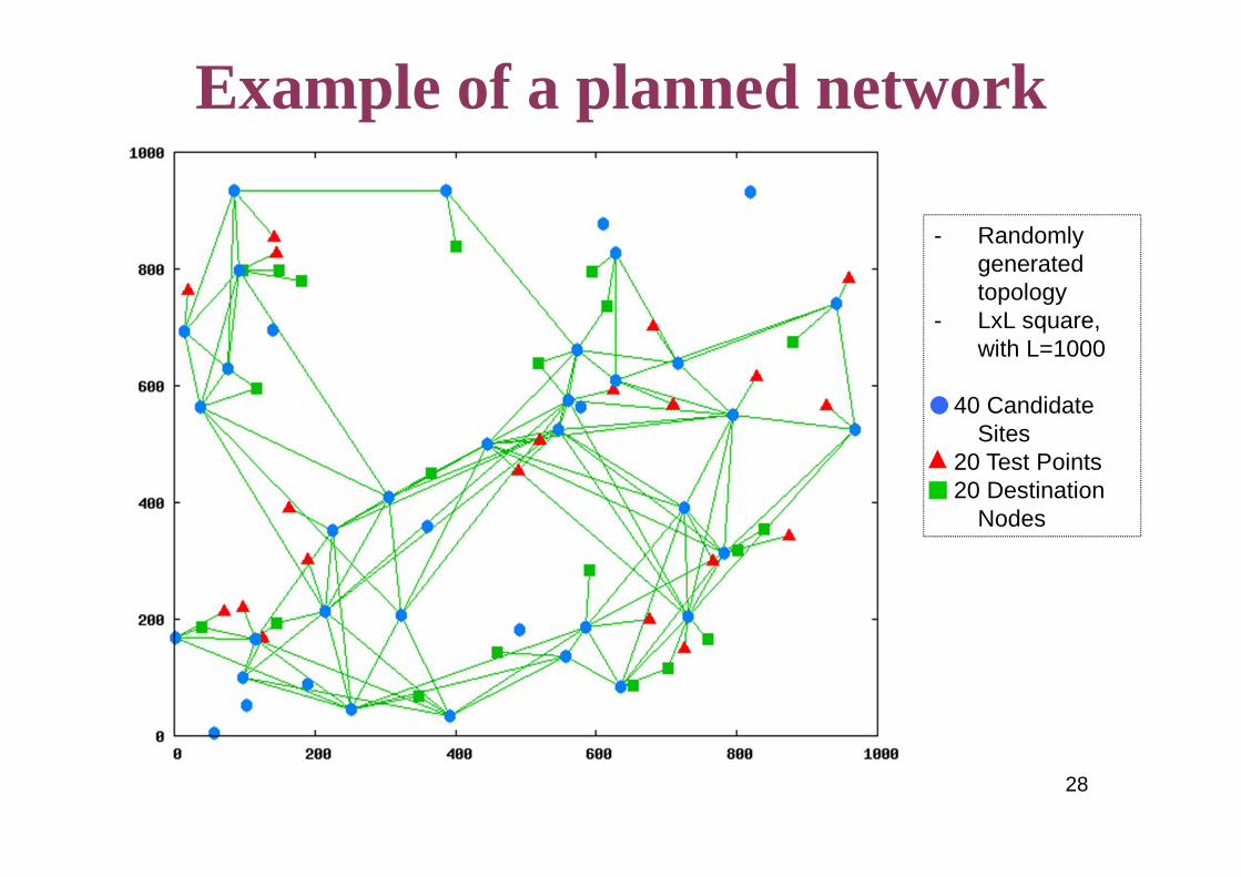
- Randomly generated topology

- LxL square, with L=1000

40 Candidate Sites

20 Test Points20 Destination

Nodes

Exampleof a plannednetwork

Network Design Applications:Service Overlay Network

� SON is an application-layer network built on top of the traditional IP-layer networks

NetworkDomain

NetworkDomain

NetworkDomain

Accessnetwork

SON

Logical link

ServiceGateway

Accessnetwork

29

What is a Service Overlay Network?

� SON is operated by an “overlay ISP”

� The SON operator owns one or more overlay nodes (also called “service gateways”) hosted in the underlying ISP domains

� Overlay nodes are interconnected by virtual overlay links that are mapped into paths of the underlying network

� SON operator purchases bandwidth for virtual links from ISPs with bilateral SLAs

� SON provides QoS guarantees to customers implementing application specific traffic management mechanisms

30

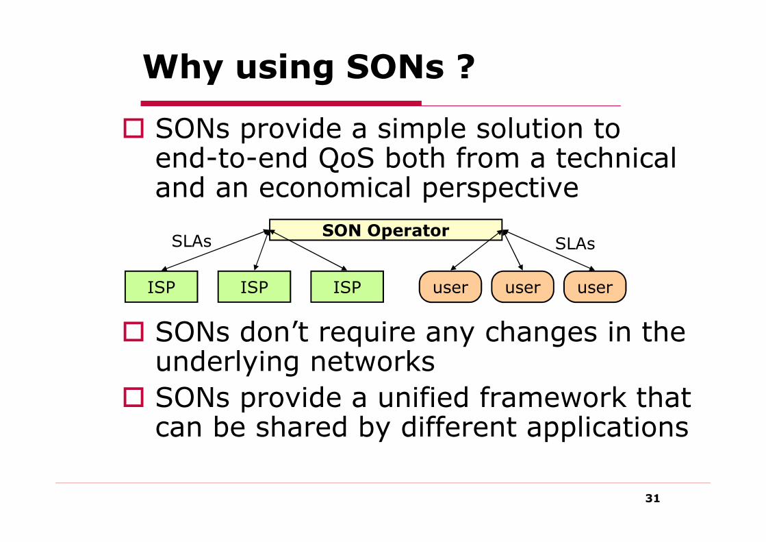
Why using SONs ?

� SONs provide a simple solution to end-to-end QoS both from a technical and an economical perspective

� SONs don’t require any changes in the underlying networks

� SONs provide a unified framework that can be shared by different applications

ISP ISPISP user user user

SON OperatorSLAs SLAs

31

� Problem Statement:� Given a set of Candidate Sites (where to install overlay nodes)

and source-destination traffic pairs:

� Goals:Deploy a SON that:

1. Minimizes the total network installation cost

2. Maximizes the profit of the SON operator

� Taking into account the SON operator’s budget

� Critical issues:� Revenue: the model must take explicitly into account the

SON operator’s revenue in the optimization procedure

� The number and location of overlay nodes are not pre-determined

� Capacity constraints on overlay links are considered

� Fast and efficient heuristics must be developed to deal with large-scale network optimization and to support periodical SON redesign based on traffic statistics measured on-line

Topology Design & Bandwidth Provisioning of SONs

32

We now illustrate an optimization framework for planning SONs

� Two mathematical programming models:

1.The first model (FCSD) minimizes the

network installation cost while providing full coverage to all users

2.The second model (PMSD) maximizes

the SON profit choosing which users to serve based on the expected gain and taking into account the budget constraint

33

Topology Design & Bandwidth Provisioning of SONs

� Two efficient heuristics to get near-optimal solutions for large-size network instances with a short computing time

1. The Cost Minimization SON Design Heuristic (H-FCSD)

2. The Profit Maximization SON Design Heuristic (H-PMSD)

34

Topology Design & Bandwidth Provisioning of SONs

Mathematical ModelsFCSD

Objective Function:(FCSD: Full-Coverage SON Design model)

NodeInstallation

cost

Accesscost

Egresscost

Overlay links bandwidth cost

Subject to:Flow Conservation constraintsAccess and Egress coverage

Coherence and Integrality constraints

PMSD

Objective Function:(PMSD: Profit Maximization SON Design

model)

SON revenue

35

Profit Maximization Model

� The SON planner may define a budget (B) to limit the economic risks in the deployment of its network:

Budget Constraint

Budget constraint

36

45

Radio planning

46

Network architecture

47

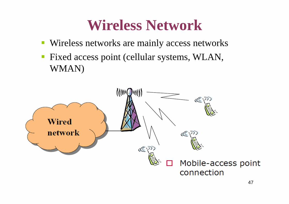
Wireless Network� Wireless networks are mainly access networks

� Fixed access point (cellular systems, WLAN, WMAN)

48

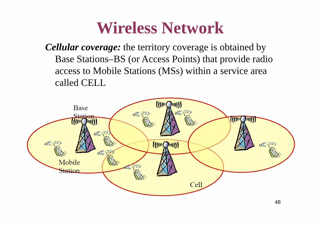
Cellular coverage: the territory coverage is obtained by Base Stations–BS (or Access Points) that provide radio access to Mobile Stations (MSs) within a service area called CELL

Wireless Network

49

What is radio planning?� When we have to install a new wireless network or

extend an existing one into a new area, we need to design the fixed and the radio parts of the network. This phase is called radio planning.

� The basic decisions that must be taken during the radio planning phase are:

– Where to install base stations (or access points, depending on the technology)

– How to configure base stations (antenna type, height, sectors orientation, maximum power, device capacity, etc.)

50

What is radio planning?� The basic decisions that must be taken during the radio planning phase are:

– Where to install base stations (or access points, depending on the technology)

– How to configure base stations (antenna type, height, sectors orientation, maximum power, device capacity, etc.)

51

Antenna positioning

� The selection of possible antenna sites depends on several technical (traffic density and distribution, ground morphology, etc.) and non-technical (electromagnetic pollution, local authority rules, agreements with building owners, etc.) issues.

� We denote with S the set of Css

� We can assume that the channel gain gij between TP i and CS j is provided by a propagation prediction tool.

52

Antenna positioning� The antenna configuration affects the signal level received

at TPs

� For each CS j we can define a set of possible antenna configurations Kj

� We can assume that the channel gain gijk between TP i and CS j depends also on configuration k.

� Based on signal quality requirement and channel gain we can evaluate if TP i can be covered by CS j with an antenna with configuration k, and define coefficients:

53

Coverage planning

� The goal of the coverage planning is to:

– Select where to install base stations

– Select antenna configurations

� To ensure that the signal level in all TPs is high enough to guarantee a good communication quality

� Note that interference is not considered here

54

Decision variables and parameters

� Decision variables:

� yjk: 0-1 decision variable that indicates if a base station with configuration k is installed in CS j

� Installation cost:

� cjk:cost related to the installation of a base station in CS j with configuration k

55

Set covering problem

Objective function:Total cost

Full coverage constraints

One configuration per site

Integrality constraints