Network Psychiatry

Network Psychiatry

Investigating models of mental constructs and disorders

with complex systems and Bayesian Artificial Intelligence

Giovanni Briganti

These defendue pour l’obtention du grade de Docteur en Sciences Medicales

Jury

Prof. Samuel Leistedt, MD, PhD, Promoteur, Universite de Mons

Prof. Paul Linkowski, MD, PhD, Co-Promoteur, Universite libre de Bruxelles

Prof. Alexandre Legrand, MD, PhD, President du Jury, Universite de Mons

Dr. Quoc Lam Vuong, PhD, Secretaire du Jury, Universite de Mons

Prof. Pierre Manneback, PhD, Universite de Mons

Prof. Christophe Lelubre, MD, PhD, Universite de Mons

Prof. Adelin Albert, PhD, Universite de Liege

Prof. Pierre Thomas, MD, PhD, Universite de Lille

Network Psychiatry

Investigating models of mental constructs and disorders with complex

systems and Bayesian Artificial Intelligence

Giovanni Briganti

Abstract

Inspired by the network approach to psychopathology, this thesis aims to investigate several

mental constructs and disorders with complex systems and Bayesian Artificial Intelligence

in order to model interactions among construct features and symptoms, evaluate their re-

spective importance in the determination of the network structure, as well as offer new

methodological perspectives to be used in network studies.

This work is organized as follows: first, an introduction to the network approach in psy-

chiatric research and potentially in clinical practice will be introduced. Second, a statistical

introduction to the network techniques, both frequentist and Bayesian will be offered to the

reader. Third, I will investigate from a network perspective several important psychiatric

constructs found in the general population. Fourth, I will translate the network approach to

psychiatric disorders using both nonclinical and clinical samples. Finally, I will discuss the

implications of this work as well as set further challenges based on my analyses.

1

List of publications

The publications resulting from this dissertation are listed below.

Briganti, G., Kempenaers, C., Braun, S., Fried, E. I., and Linkowski, P. (2018). Network

analysis of empathy items from the interpersonal reactivity index in 1973 young adults.

Psychiatry Research, 265:87–92.

Briganti, G., Fried, E. I., and Linkowski, P. (2019). Network analysis of Contingencies

of Self-Worth Scale in 680 university students. Psychiatry Research, 272:252–257.

Briganti, G. and Linkowski, P. (2019). Exploring network structure and central items

of the narcissistic personality inventory. International Journal of Methods in Psychiatric

Research, e1810.

Briganti, G. and Linkowski, P. (2019). Item and domain network structures of the Re-

silience Scale for Adults in 675 university students. Epidemiology and Psychiatric Sciences,

pages 1–9.

Briganti, G. and Linkowski, P. (2019). Network approach to items and domains from

thetoronto alexithymia scale. Psychological Reports, page 0033294119889586.

Briganti, G., Scutari, M., and Linkowski, P. (2020). Network structures of symptoms

from the Zung depression scale. Psychological Reports, page 0033294120942116.

Briganti, G. and Linkowski, P. (2019). Une nouvelle approche ontologique et statis-

tiquedes constructions et maladies mentales : introduction a la psychiatrie des networks.

PsyArXiv

Briganti, G., and Linkowski, P. (2020). A machine learning approach to alexithymia

2

components. Psychiatria Danubina, Sep;32(Suppl 1):180-187.

Briganti, G., Williams, D.R., Mulder, J., and Linkowski P. (2020). Bayesian network

structure and predictability of autistic traits. accepted for publication Psychological Reports.

Briganti, G., Kornreich, C., and Linkowski, P. (2020). A network structure of manic

symptoms. submitted.

Briganti, G., Hubain, P., Kornreich, C., and Linkowski, P. (2020). Investigating the het-

erogeneity of psychiatric symptomatology using community detection algorithms. accepted

in Acta Psychiatrica Belgica.

Briganti G., and Scutari M. (2020). An Introduction to Bayesian Artificial Intelligence

in Medicine. submitted.

3

List of abbreviations

A: Appearance

AC: Academic Competence

AI: Artificial Intelligence

ANN: Artificial Neural Network

AQ: Alexithymia Questionnaire (in Chapter 9); Autistic Spectrum Quotient (in Chapter 10).

ASD: Autism Spectrum Disorders

BAI: Bayesian Artificial Intelligence

BF: Bayes Factor

BGGM: Bayesian Gaussian Graphical Model

BN: Bayesian Network

BVAQ: Bermond-Vorst Alexithymia Questionnaire

C: Competition

CFA: Confirmatory Factor Analysis

CFI: Comparative Fit Index

CPM: Clique Percolation Method

CS: Centrality-stability coefficient

CSWS: Contingencies of Self-Worth Scale

DAG: Directed Acyclic Graph

DSM-5: Diagnostic and Statistical Manual of mental disorders (5th edition)

EBIC: Extended Bayesian Information Criterion

4

EC: Empathic Concern

EGA: Exploratory Graph Analysis

EI: Expected Influence

EFA: Exploratory Factor Analysis

FS: Fantasy Scale (in Chapter 4); Family Support (in Chapter 5)

GGM: Gaussian Graphical Model

GL: God’s Love

GVAR: Graphical Vector Autoregressive Model

HRSD: Hamilton Rating Scale for Depression

IC: Inductive Causation algorithm

ICD-10: International Classification of Diseases (10th revision)

IM: Ising Model

IRI: Interpersonal Reactivity Index

LASSO: Least Absolute Shrinkage and Selection Operator

MDD: Major Depressive Disorder

MGM: Mixed Graphical Model

ML: Machine Learning

NCT: Network Comparison Test

NPI: Narcissistic Personality Inventory

OA: Other’s Approval

PC: Peter & Clark algorithm

PD: Personal Distress

PT: Perspective Taking

PTSD: Post-Traumatic Stress Disorder

R: R for statistical computing

RMSEA: Root Mean Square Error of Approximation

RSA: Resilience Scale for Adults

5

SRMSR: Standardized Root Mean Square Residual

SDS: Self-rating Depression Scale

TAS: Toronto Alexithymia Scale

TSIA: Toronto Structured Interview for Alexithymia

V: Virtue

YMRS: Young Mania Rating Scale

6

Contents

I An Introduction to Network Psychiatry 14

1 Network psychiatry: state of the art and challenges 15

1.1 Introduction . . . . . . . . . . . . . . . . . . . . . . . . . . . . . . . . . . . . 15

1.2 Structure and composition of a psychiatric network . . . . . . . . . . . . . . 20

1.2.1 Elements composing a network . . . . . . . . . . . . . . . . . . . . . 20

1.2.2 Types of networks . . . . . . . . . . . . . . . . . . . . . . . . . . . . 21

1.3 An introduction to the estimation of a psychiatric network . . . . . . . . . . 24

1.3.1 Conditional dependence and independence . . . . . . . . . . . . . . . 25

1.3.2 Partial correlations . . . . . . . . . . . . . . . . . . . . . . . . . . . . 25

1.3.3 Gaussian Graphical Model, Ising Model, Mixed Graphical Model . . . 26

1.3.4 Regularization . . . . . . . . . . . . . . . . . . . . . . . . . . . . . . . 26

1.3.5 Bayesian estimation of the Gaussian Graphical Model . . . . . . . . . 27

1.4 Network inference . . . . . . . . . . . . . . . . . . . . . . . . . . . . . . . . . 27

1.4.1 Centrality and redundancy . . . . . . . . . . . . . . . . . . . . . . . . 27

1.4.2 Symptom prediction . . . . . . . . . . . . . . . . . . . . . . . . . . . 29

1.4.3 Community detection in Networks . . . . . . . . . . . . . . . . . . . . 30

1.4.4 Network of domains . . . . . . . . . . . . . . . . . . . . . . . . . . . . 30

1.5 Discussion: state of the art and challenges of the network approach in clinical

practice . . . . . . . . . . . . . . . . . . . . . . . . . . . . . . . . . . . . . . 32

7

2 A primer on Bayesian Artificial Intelligence and networks 34

2.1 Introduction . . . . . . . . . . . . . . . . . . . . . . . . . . . . . . . . . . . . 34

2.2 Probabilistic reasoning . . . . . . . . . . . . . . . . . . . . . . . . . . . . . . 36

2.3 Bayesian thinking in machine learning . . . . . . . . . . . . . . . . . . . . . 37

2.4 Bayesian Networks . . . . . . . . . . . . . . . . . . . . . . . . . . . . . . . . 39

2.4.1 The use of graphs to represent interactions among entities . . . . . . 39

2.4.2 Directed Acyclic Graphs . . . . . . . . . . . . . . . . . . . . . . . . . 41

2.5 Difference between neural networks and Bayesian networks . . . . . . . . . . 43

2.6 Structure learning of Bayesian networks . . . . . . . . . . . . . . . . . . . . . 44

2.6.1 The Markov property . . . . . . . . . . . . . . . . . . . . . . . . . . . 44

2.6.2 Markov blankets . . . . . . . . . . . . . . . . . . . . . . . . . . . . . 45

2.6.3 Bayesian networks and Causality . . . . . . . . . . . . . . . . . . . . 46

2.6.4 Structure learning algorithms . . . . . . . . . . . . . . . . . . . . . . 47

2.7 Discussion: applications and limitations of Bayesian Artificial Intelligence in

Medicine . . . . . . . . . . . . . . . . . . . . . . . . . . . . . . . . . . . . . . 48

3 A primer on undirected network models 51

3.1 Introduction . . . . . . . . . . . . . . . . . . . . . . . . . . . . . . . . . . . . 51

3.2 Estimating network models from cross-sectional data . . . . . . . . . . . . . 52

3.2.1 Network components in undirected graphical models . . . . . . . . . 52

3.2.2 The Gaussian Graphical Model . . . . . . . . . . . . . . . . . . . . . 53

3.2.3 Bayesian estimation of the Gaussian Graphical Model . . . . . . . . . 53

3.2.4 The Ising Model . . . . . . . . . . . . . . . . . . . . . . . . . . . . . 55

3.2.5 Interpreting undirected network models in cross-sectional data sets . 57

3.3 Estimating network models from several time points . . . . . . . . . . . . . . 57

3.3.1 Granger causality . . . . . . . . . . . . . . . . . . . . . . . . . . . . . 58

3.3.2 The Graphical Vector Autoregressive Model . . . . . . . . . . . . . . 58

3.4 Network inference . . . . . . . . . . . . . . . . . . . . . . . . . . . . . . . . . 59

8

3.4.1 Centrality . . . . . . . . . . . . . . . . . . . . . . . . . . . . . . . . . 59

3.4.2 Node predictability . . . . . . . . . . . . . . . . . . . . . . . . . . . . 60

3.5 Stability and accuracy . . . . . . . . . . . . . . . . . . . . . . . . . . . . . . 61

3.6 Conclusion . . . . . . . . . . . . . . . . . . . . . . . . . . . . . . . . . . . . . 62

II A network approach to mental constructs 63

4 A network model of empathy 64

4.1 Introduction . . . . . . . . . . . . . . . . . . . . . . . . . . . . . . . . . . . . 65

4.2 Method . . . . . . . . . . . . . . . . . . . . . . . . . . . . . . . . . . . . . . 67

4.2.1 Data set . . . . . . . . . . . . . . . . . . . . . . . . . . . . . . . . . . 67

4.2.2 Network analysis . . . . . . . . . . . . . . . . . . . . . . . . . . . . . 70

4.3 Results . . . . . . . . . . . . . . . . . . . . . . . . . . . . . . . . . . . . . . . 73

4.3.1 Empathy network . . . . . . . . . . . . . . . . . . . . . . . . . . . . . 73

4.3.2 Network inference . . . . . . . . . . . . . . . . . . . . . . . . . . . . . 75

4.3.3 Network accuracy and stability . . . . . . . . . . . . . . . . . . . . . 77

4.4 Discussion . . . . . . . . . . . . . . . . . . . . . . . . . . . . . . . . . . . . . 77

5 A network model of self-worth 81

5.1 Introduction . . . . . . . . . . . . . . . . . . . . . . . . . . . . . . . . . . . . 81

5.2 Method . . . . . . . . . . . . . . . . . . . . . . . . . . . . . . . . . . . . . . 84

5.2.1 Participants . . . . . . . . . . . . . . . . . . . . . . . . . . . . . . . . 84

5.2.2 Measurement . . . . . . . . . . . . . . . . . . . . . . . . . . . . . . . 84


5.3 Results . . . . . . . . . . . . . . . . . . . . . . . . . . . . . . . . . . . . . . . 90

5.3.1 Descriptive statistics . . . . . . . . . . . . . . . . . . . . . . . . . . . 90

5.3.2 Network stability . . . . . . . . . . . . . . . . . . . . . . . . . . . . . 90


9

5.4 Discussion . . . . . . . . . . . . . . . . . . . . . . . . . . . . . . . . . . . . . 93

6 A network model of resilience 97

6.1 Introduction . . . . . . . . . . . . . . . . . . . . . . . . . . . . . . . . . . . . 98

6.2 Method . . . . . . . . . . . . . . . . . . . . . . . . . . . . . . . . . . . . . . 101

6.2.1 Participants . . . . . . . . . . . . . . . . . . . . . . . . . . . . . . . . 101

6.2.2 Measurement . . . . . . . . . . . . . . . . . . . . . . . . . . . . . . . 102


6.3 Results . . . . . . . . . . . . . . . . . . . . . . . . . . . . . . . . . . . . . . . 106

6.3.1 Item network . . . . . . . . . . . . . . . . . . . . . . . . . . . . . . . 106

6.3.2 Six-domain network . . . . . . . . . . . . . . . . . . . . . . . . . . . . 106



6.3.5 Four-domain network . . . . . . . . . . . . . . . . . . . . . . . . . . . 109

6.4 Discussion . . . . . . . . . . . . . . . . . . . . . . . . . . . . . . . . . . . . . 110

7 A network model of narcissism 114

7.1 Introduction . . . . . . . . . . . . . . . . . . . . . . . . . . . . . . . . . . . . 114

7.2 Method . . . . . . . . . . . . . . . . . . . . . . . . . . . . . . . . . . . . . . 117

7.2.1 Participants . . . . . . . . . . . . . . . . . . . . . . . . . . . . . . . . 117

7.2.2 Measurement . . . . . . . . . . . . . . . . . . . . . . . . . . . . . . . 117

7.3 Network analysis . . . . . . . . . . . . . . . . . . . . . . . . . . . . . . . . . 122

7.3.1 Network estimation . . . . . . . . . . . . . . . . . . . . . . . . . . . . 122



7.4 Results . . . . . . . . . . . . . . . . . . . . . . . . . . . . . . . . . . . . . . . 124

7.4.1 Participants . . . . . . . . . . . . . . . . . . . . . . . . . . . . . . . . 124

7.4.2 Network of narcissism . . . . . . . . . . . . . . . . . . . . . . . . . . 124

10



7.5 Discussion . . . . . . . . . . . . . . . . . . . . . . . . . . . . . . . . . . . . . 127

8 A network model of alexithymia without fantasizing 130

8.1 Introduction . . . . . . . . . . . . . . . . . . . . . . . . . . . . . . . . . . . . 131

8.2 Method . . . . . . . . . . . . . . . . . . . . . . . . . . . . . . . . . . . . . . 134

8.3 Data set . . . . . . . . . . . . . . . . . . . . . . . . . . . . . . . . . . . . . . 134

8.4 Measurement . . . . . . . . . . . . . . . . . . . . . . . . . . . . . . . . . . . 134


8.5 Results . . . . . . . . . . . . . . . . . . . . . . . . . . . . . . . . . . . . . . . 138

8.5.1 Item network . . . . . . . . . . . . . . . . . . . . . . . . . . . . . . . 138

8.5.2 Three-domain network . . . . . . . . . . . . . . . . . . . . . . . . . . 140



8.5.5 Four-domain network . . . . . . . . . . . . . . . . . . . . . . . . . . . 141

8.6 Discussion . . . . . . . . . . . . . . . . . . . . . . . . . . . . . . . . . . . . . 143

9 A network model of alexithymia with fantasizing 146

9.1 Introduction . . . . . . . . . . . . . . . . . . . . . . . . . . . . . . . . . . . . 146

9.2 Method . . . . . . . . . . . . . . . . . . . . . . . . . . . . . . . . . . . . . . 150

9.2.1 Data set . . . . . . . . . . . . . . . . . . . . . . . . . . . . . . . . . . 150

9.2.2 Measurement . . . . . . . . . . . . . . . . . . . . . . . . . . . . . . . 150


9.3 Results . . . . . . . . . . . . . . . . . . . . . . . . . . . . . . . . . . . . . . . 153

9.3.1 Partial correlation network . . . . . . . . . . . . . . . . . . . . . . . . 153

9.3.2 Directed Acyclic Graph . . . . . . . . . . . . . . . . . . . . . . . . . . 157

9.4 Discussion . . . . . . . . . . . . . . . . . . . . . . . . . . . . . . . . . . . . . 158

11

10 A network model of autistic traits 161

10.1 Introduction . . . . . . . . . . . . . . . . . . . . . . . . . . . . . . . . . . . . 161

10.2 Method . . . . . . . . . . . . . . . . . . . . . . . . . . . . . . . . . . . . . . 165

10.2.1 Data set . . . . . . . . . . . . . . . . . . . . . . . . . . . . . . . . . . 165

10.2.2 Measurement . . . . . . . . . . . . . . . . . . . . . . . . . . . . . . . 166


10.3 Results . . . . . . . . . . . . . . . . . . . . . . . . . . . . . . . . . . . . . . . 167

10.3.1 Partial correlation network . . . . . . . . . . . . . . . . . . . . . . . . 167

10.3.2 Node predictability . . . . . . . . . . . . . . . . . . . . . . . . . . . . 169

10.3.3 Sex differences . . . . . . . . . . . . . . . . . . . . . . . . . . . . . . . 169

10.4 Discussion . . . . . . . . . . . . . . . . . . . . . . . . . . . . . . . . . . . . . 173

III A network approach to mental disorders 175

11 A network model of depressive symptoms in a student sample 176

11.1 Introduction . . . . . . . . . . . . . . . . . . . . . . . . . . . . . . . . . . . . 177

11.2 Method . . . . . . . . . . . . . . . . . . . . . . . . . . . . . . . . . . . . . . 179

11.2.1 Participants . . . . . . . . . . . . . . . . . . . . . . . . . . . . . . . . 179

11.2.2 Measurement . . . . . . . . . . . . . . . . . . . . . . . . . . . . . . . 179


11.3 Results . . . . . . . . . . . . . . . . . . . . . . . . . . . . . . . . . . . . . . . 183

11.3.1 Regularized partial correlation network . . . . . . . . . . . . . . . . . 183

11.3.2 DAG . . . . . . . . . . . . . . . . . . . . . . . . . . . . . . . . . . . . 184

11.4 Discussion . . . . . . . . . . . . . . . . . . . . . . . . . . . . . . . . . . . . . 185

12 A network model of mania 188

12.1 Introduction . . . . . . . . . . . . . . . . . . . . . . . . . . . . . . . . . . . . 188

12.2 Method . . . . . . . . . . . . . . . . . . . . . . . . . . . . . . . . . . . . . . 192

12

12.2.1 Ethical approval . . . . . . . . . . . . . . . . . . . . . . . . . . . . . . 192

12.2.2 Data sets . . . . . . . . . . . . . . . . . . . . . . . . . . . . . . . . . 193

12.2.3 Network Analysis . . . . . . . . . . . . . . . . . . . . . . . . . . . . . 194

12.3 Results . . . . . . . . . . . . . . . . . . . . . . . . . . . . . . . . . . . . . . . 197

12.3.1 Cross-sectional networks . . . . . . . . . . . . . . . . . . . . . . . . . 197


12.3.3 Temporal network . . . . . . . . . . . . . . . . . . . . . . . . . . . . . 203

12.4 Discussion . . . . . . . . . . . . . . . . . . . . . . . . . . . . . . . . . . . . . 205

IV Overcoming challenges in network psychiatry 208

13 Investigating the heterogeneity of psychiatric symptomatology using com-

munity detection algorithms 209

13.1 Introduction . . . . . . . . . . . . . . . . . . . . . . . . . . . . . . . . . . . . 210

13.2 Method . . . . . . . . . . . . . . . . . . . . . . . . . . . . . . . . . . . . . . 215

13.2.1 Ethical approval . . . . . . . . . . . . . . . . . . . . . . . . . . . . . . 215

13.2.2 Data sets . . . . . . . . . . . . . . . . . . . . . . . . . . . . . . . . . 215

13.2.3 Network Analysis . . . . . . . . . . . . . . . . . . . . . . . . . . . . . 216

13.2.4 Community detection . . . . . . . . . . . . . . . . . . . . . . . . . . . 218

13.2.5 Bridge centrality . . . . . . . . . . . . . . . . . . . . . . . . . . . . . 223

13.3 Results . . . . . . . . . . . . . . . . . . . . . . . . . . . . . . . . . . . . . . . 223

13.3.1 Community detection . . . . . . . . . . . . . . . . . . . . . . . . . . . 223

13.3.2 Bridge centrality . . . . . . . . . . . . . . . . . . . . . . . . . . . . . 229

13.4 Discussion . . . . . . . . . . . . . . . . . . . . . . . . . . . . . . . . . . . . . 229

14 Discussion 235

14.1 Future directions . . . . . . . . . . . . . . . . . . . . . . . . . . . . . . . . . 238

14.2 Conclusion . . . . . . . . . . . . . . . . . . . . . . . . . . . . . . . . . . . . . 239

13

Part I

An Introduction to Network

Psychiatry

14

Chapter 1

Network psychiatry: state of the art

and challenges

Abstract

The network approach is enjoying increasing success in psychiatry and computa-

tional neuroscience. This new methodology, resulting from the translation of models of

statistical physics into medicine, grants a new ontological view on mental disorders, by

defining them as complex systems emerging from the interconnection between different

symptoms. This work offers an introduction, both theoretical and methodological, to

the potential of this approach to improve the diagnosis and treatment of psychiatric

disorders, by providing some examples of application explored in clinical research.

1.1 Introduction

The word “symptom” is defined as a “subjective phenomenon which translates morbid states

and which is linked to the functional or lesional disorders which determine it”. In current

psychiatric practice, the complaints reported by a patient to the clinician taking care of

him have been categorized as “symptoms”, a definition exemplified in diagnostic reference

manuals, such as the ICD-10 or the DSM-5. In somatic medicine, the presence of a symptom

15

implies the presence of an underlying disease, due to a uni- or multi-factorial etiology most

often identified.

In psychiatry, however, the concept of “mental illness”, although still strongly repre-

sented in the forensic field (I am thinking in particular of the Belgian law of June 26, 1990

relating to the psychiatric hold of the mentally ill), gradually gives way to the concept of

“mental disorder”, as described by the DSM-V (American Psychiatric Association, 2013) and

referring to a “syndrome”. The syndrome is in turn defined as a “set of several symptoms

or signs related to a given pathological condition and allowing, by their grouping, to guide

the diagnosis“: it is therefore an ecosystem of entities detected by the clinician or declared

to the latter; this ecosystem carries an empirical meaning, but for an unknown reason. For

most psychiatric pathologies, however, the classic etiopathogenic approach used in medi-

cal research has proven unsuccessful (Borsboom and Cramer, 2013): in psychiatry, one can

rarely identify a cause which, completely eliminated, makes the entire the symptomatological

presentation of the patient disappear, such as the effect that administration of an antibiotic

would have on an infection caused by a particular germ.

However, classic psychometrics (the field common to psychiatry and psychology which

aims to measure mental entities, both normal and pathological) has nowadays a very large

majority of measurement tools that conceive of mental disorders as being the consequence

of a common cause. This approach, which has been widely used in recent decades and well

consolidated in the scientific literature, is known as the “latent variable model” (Marsman

et al., 2018). According to the latent variables model, the symptoms encountered in clinical

practice are elements which can be measured, but which constitute only a passive reflection

of the pathology in question; like a cough during pneumonia, the psychiatric symptom does

not represent a component which causes the pathology, but is the measured effect of the

pathology itself.

A decade ago, some work put forward the hypothesis that a central cause for mental

disorders cannot be found because there is no central cause; instead of being caused by an

16

Figure 1.1: Latent variable model. A latent variable (C) causes 9 symptoms.

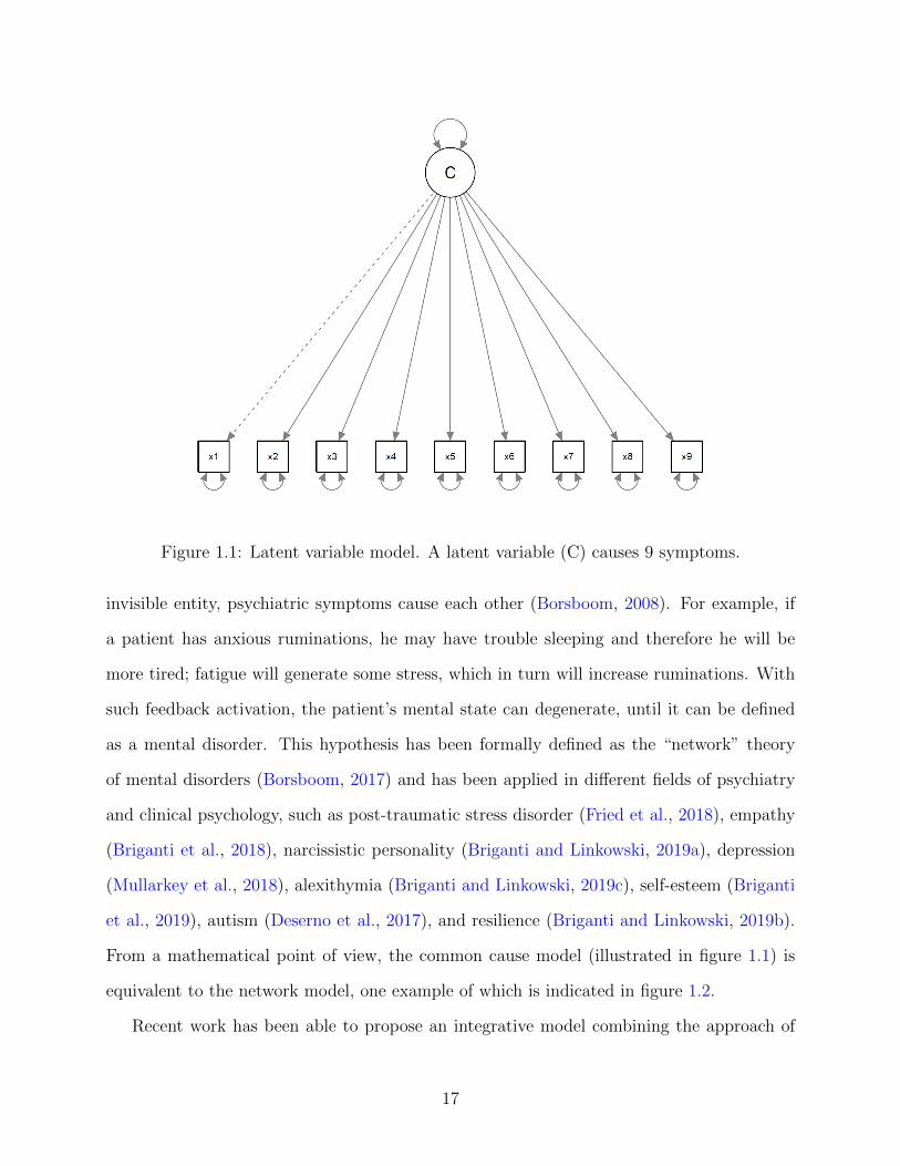
invisible entity, psychiatric symptoms cause each other (Borsboom, 2008). For example, if

a patient has anxious ruminations, he may have trouble sleeping and therefore he will be

more tired; fatigue will generate some stress, which in turn will increase ruminations. With

such feedback activation, the patient’s mental state can degenerate, until it can be defined

as a mental disorder. This hypothesis has been formally defined as the “network” theory

of mental disorders (Borsboom, 2017) and has been applied in different fields of psychiatry

and clinical psychology, such as post-traumatic stress disorder (Fried et al., 2018), empathy

(Briganti et al., 2018), narcissistic personality (Briganti and Linkowski, 2019a), depression

(Mullarkey et al., 2018), alexithymia (Briganti and Linkowski, 2019c), self-esteem (Briganti

et al., 2019), autism (Deserno et al., 2017), and resilience (Briganti and Linkowski, 2019b).

From a mathematical point of view, the common cause model (illustrated in figure 1.1) is

equivalent to the network model, one example of which is indicated in figure 1.2.

Recent work has been able to propose an integrative model combining the approach of

17

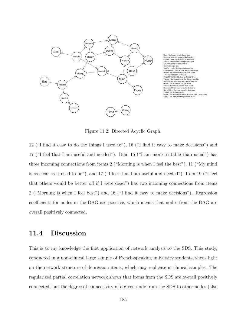
Figure 1.2: The network model. Variables (nodes) interact through connections (edges).Positive edges are colored in blue, negative edges are colored in red. The correspondingthickness of an edge denotes its intensity (weight).

18

latent variables with the network approach: in this approach, called generalized network

psychometrics (Epskamp et al., 2017b) the symptoms can be caused by different latent

variables and interact with each other. This approach has proven useful in simplifying the

analysis of networks based on psychometric scales, where different dimensions are represented

by several redundant items. Once the redundancy is limited by representing the symptoms by

the latent variables that it measures, for example a particular domain of a mental construct,

such as the contribution of self-opinion in the construct of self-esteem (Briganti et al., 2019),

an interaction between the different latent variables is observed. Some work has been able

to demonstrate that new tools, such as exploratory graphical analysis (Golino and Epskamp,

2017), specifically designed for the detection of domains in networks (translate “factors” in

the approach by latent variables) is capable of detecting the correct number of dimensions

in a sample; if the number detected is not the same, a new model is proposed which is better

suited to the sample data.

The aim of this work is to offer a general introduction to network psychiatry, paying

particular attention to the implications that the development of this approach can have on

the diagnosis and treatment of mental disorders. I detail the challenges, opportunities and

main criticisms that have been described in the literature in this area, which has evolved

rapidly in the last decade. I will first describe the structure and composition of a psychiatric

network. Next, I will detail the different processes for estimating a psychiatric network.

Third, I will detail the different measures used to interpret the results of a network, as well

as their stability and accuracy. Finally, I will discuss the main applications that this approach

could develop in current clinical practice. The main criticisms of the network approach will

be integrated as the different methodologies are introduced.

19

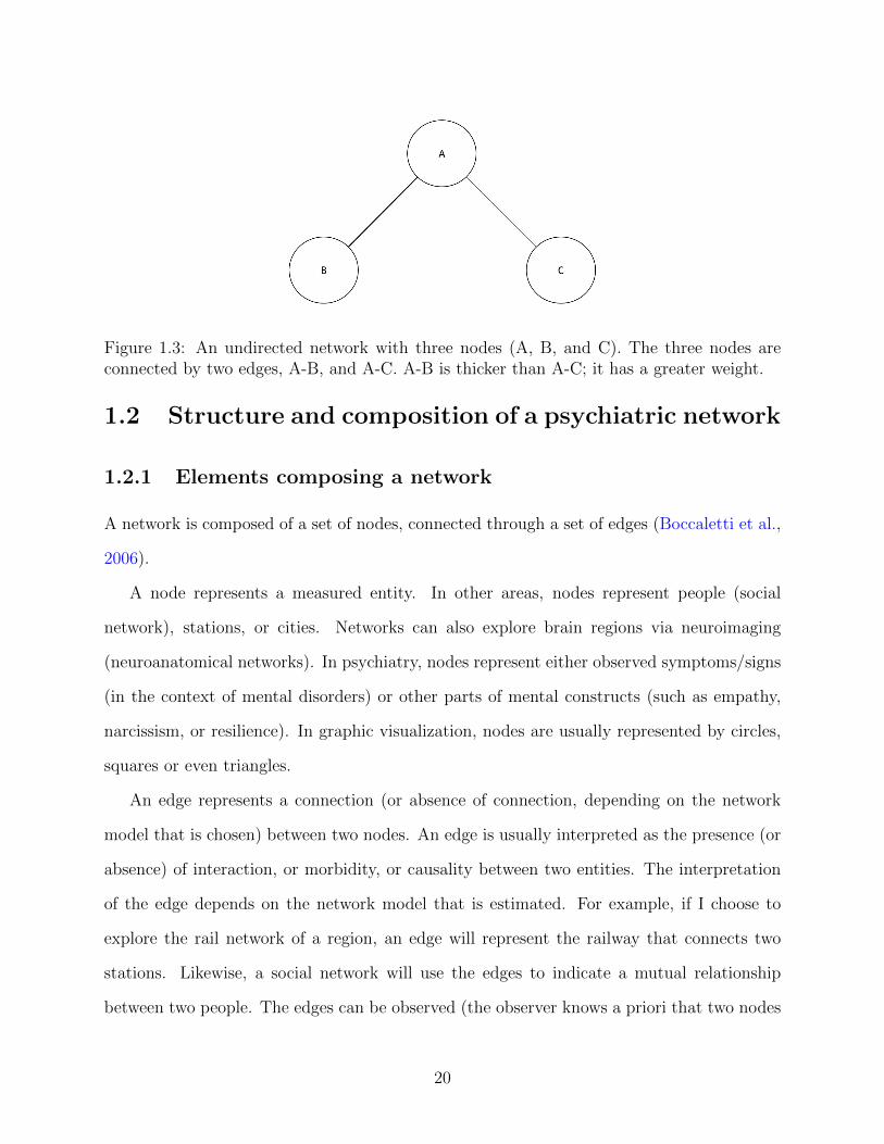
Figure 1.3: An undirected network with three nodes (A, B, and C). The three nodes areconnected by two edges, A-B, and A-C. A-B is thicker than A-C; it has a greater weight.

1.2 Structure and composition of a psychiatric network

1.2.1 Elements composing a network

A network is composed of a set of nodes, connected through a set of edges (Boccaletti et al.,

2006).

A node represents a measured entity. In other areas, nodes represent people (social

network), stations, or cities. Networks can also explore brain regions via neuroimaging

(neuroanatomical networks). In psychiatry, nodes represent either observed symptoms/signs

(in the context of mental disorders) or other parts of mental constructs (such as empathy,

narcissism, or resilience). In graphic visualization, nodes are usually represented by circles,

squares or even triangles.

An edge represents a connection (or absence of connection, depending on the network

model that is chosen) between two nodes. An edge is usually interpreted as the presence (or

absence) of interaction, or morbidity, or causality between two entities. The interpretation

of the edge depends on the network model that is estimated. For example, if I choose to

explore the rail network of a region, an edge will represent the railway that connects two

stations. Likewise, a social network will use the edges to indicate a mutual relationship

between two people. The edges can be observed (the observer knows a priori that two nodes

20

are connected) or else unobserved (the presence or absence of a relationship between two

nodes must therefore be tested, by defining a null hypothesis and an alternative hypothesis).

1.2.2 Types of networks

There are different types of networks. Below I will detail the types of networks most used

in psychiatry.

Undirected network, weighted or unweighted

An undirected network is a structure with nodes connected by edges whose direction is

unknown. An example of an undirected network is illustrated in figure 1.3. The edge A-B

connecting nodes A and B, could, in an undirected network, assume 3 possible directions:

A to B, B to A, or symmetrically from A to B and vice-versa. The edges of an undirected

network can have a weight, reflecting the relative importance of one edge compared to others.

The weight of the edge is most often represented by a thicker link. Networks containing

weights are called weighted networks; weightless networks are unweighted.

To understand the importance of weighting, let’s take the example of three known symp-

toms of depression (Zung, 1965) that could underlie the figure 1.3: insomnia (A), fatigue (B),

and suicidal ideation (C). Insomnia could be linked to suicidal ideation as well as fatigue, but

its connection to fatigue is much more clinically important than to suicidal ideation. The

edge weights are used precisely to express this difference between the connections within a

network.

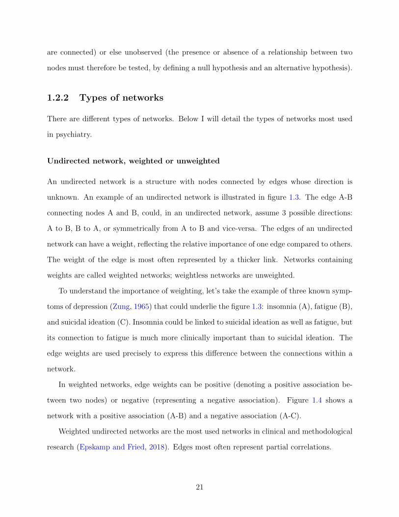
In weighted networks, edge weights can be positive (denoting a positive association be-

tween two nodes) or negative (representing a negative association). Figure 1.4 shows a

network with a positive association (A-B) and a negative association (A-C).

Weighted undirected networks are the most used networks in clinical and methodological

research (Epskamp and Fried, 2018). Edges most often represent partial correlations.

21

Figure 1.4: An undirected weighted network with three nodes (A, B, and C). The threenodes are connected by two edges, A-B and A-C. A-B denotes a positive connection. A-Cdenotes a negative connection. A-B has a greater weight than A-C.

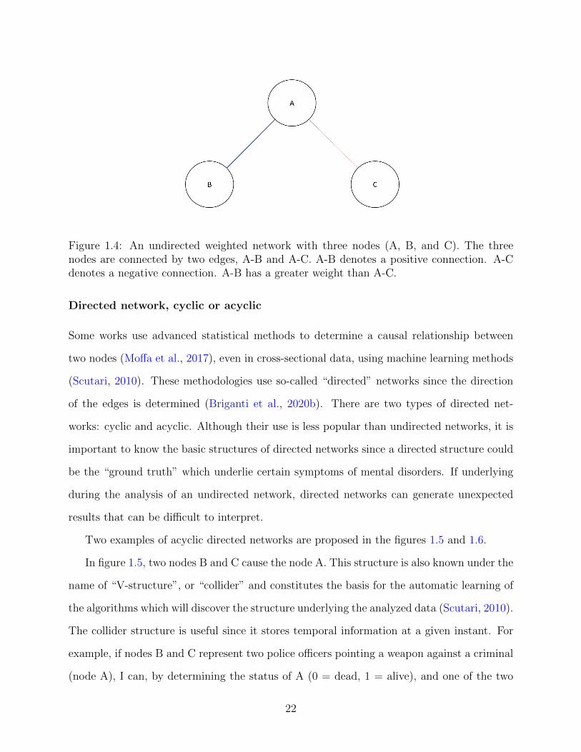
Directed network, cyclic or acyclic

Some works use advanced statistical methods to determine a causal relationship between

two nodes (Moffa et al., 2017), even in cross-sectional data, using machine learning methods

(Scutari, 2010). These methodologies use so-called “directed” networks since the direction

of the edges is determined (Briganti et al., 2020b). There are two types of directed net-

works: cyclic and acyclic. Although their use is less popular than undirected networks, it is

important to know the basic structures of directed networks since a directed structure could

be the “ground truth” which underlie certain symptoms of mental disorders. If underlying

during the analysis of an undirected network, directed networks can generate unexpected

results that can be difficult to interpret.

Two examples of acyclic directed networks are proposed in the figures 1.5 and 1.6.

In figure 1.5, two nodes B and C cause the node A. This structure is also known under the

name of “V-structure”, or “collider” and constitutes the basis for the automatic learning of

the algorithms which will discover the structure underlying the analyzed data (Scutari, 2010).

The collider structure is useful since it stores temporal information at a given instant. For

example, if nodes B and C represent two police officers pointing a weapon against a criminal

(node A), I can, by determining the status of A (0 = dead, 1 = alive), and one of the two

22

Figure 1.5: An acyclic directed network composed of three nodes A, B, and C. B and Ccause A. This is commonly defined as a collider situation.

Figure 1.6: An acyclic directed network composed of three nodes A, B, and C. A causes B,B causes C.

23

Figure 1.7: A cyclic directed network composed of three nodes A, B, and C. A causes B, Bcauses C, and C causes A.

police officers (0 = did not fire, 1 = fired), infer the status of the other police officer.

In figure 1.6, A cause B which in turn causes C. C does not cause A, which leaves the

loop open.

The loop is however closed in the figure 1.7, representing a cyclic directed network.

Cyclic networks are most often encountered in time series, where repeated measurements of

psychiatric parameters are made to control the mental state. Cyclical directed networks could

be useful in order to show the existence of a “critical slowing down” of symptoms: during the

deterioration of a mental state, the prediction between the symptoms in a network becomes

more concrete (Wichers and Groot, 2016).

1.3 An introduction to the estimation of a psychiatric

network

This constitutes a brief and clinical introduction to the estimation of network models used in

clinical research. A statistical introduction of the methods used in this thesis can be found

in Chapters 2 and 3.

24

1.3.1 Conditional dependence and independence

The presence of an edge in a network can mean the presence or absence of a connection

between two nodes. This depends on whether the estimation of a network aims to detect the

presence of a conditional dependence or a conditional independence (Williams et al., 2019).

A conditional dependence is understood as an association between two variables when a

third variable is set. Conditional independence is understood as the absence of association

between two variables when a third variable is fixed at given levels (Epskamp et al., 2017b).

1.3.2 Partial correlations

Most often, the edges between the nodes are estimated in the form of partial correlations,

one of the statistical translation of the theoretical concept of conditional dependence relation

(Epskamp and Fried, 2018). A network of partial correlations will look like the models

proposed in the figures 1.2 and 1.4: a weighted network not directed. The partial correlations

will be positive or negative, reflecting a corresponding association between the nodes.

How to interpret the presence of a positive partial correlation between two variables X

and Y found in a network of psychiatric symptoms such as collected with self-administered

scales? From a statistical point of view, I can affirm that, if a partial correlation is present

between X and Y, that implies that, by controlling all the other variables of the network, a

connection exists between the two nodes (Briganti et al., 2018).

To translate this mathematical explanation into clinical practice, a possible interpretation

is as follows: by controlling all the other symptoms, if X and Y share a connection, this means

that in the observed sample the average response of the observed group to question X will

be able to predict that of Y and vice-versa, since the network is undirected (Briganti et al.,

2019). In practice, if I observe a partial correlation between two symptoms insomnia and

fatigue, I can deduce that if the observed group has on average significant insomnia, it will

also present significant fatigue, controlling the levels of other network symptoms.

25

1.3.3 Gaussian Graphical Model, Ising Model, Mixed Graphical

Model

All the partial correlations of a network are determined at the same time by the estimation

of a Gaussian Graphic Model (GGM), applicable for continuous data (or comparable to con-

tinuous) (Williams, 2018a). The GGM (the network itself) is estimated as the inverse of the

covariance matrix derived from the collected symptom data set. The alternative for binary

variable of the GGM is Ising’s model, derived from statistical physics and adapted in psychi-

atry (van Borkulo et al., 2014), but rarely used in empirical work (Briganti and Linkowski,

2019a). Depending on the type of variables included (for example, if a binary variable such

as the gender of the participants is added to a continuous database), Mixed Graphic Models

(MGM) can be used (Haslbeck and Waldorp, 2016). The GGM is nevertheless the model

used predominantly in the literature.

GGM is easy to understand, especially if it is used to study a mental disorder. Let

y = (y1, ..., yp)> be any normal multivariate vector. Without loss of information, the data are

considered to be centered with an average vector of 0 and a covariance matrix Σ. The inverse

of the covariance matrix Θ = Σ−1 is targeted in network analysis, since by standardizing

the off-diagonal elements of the matrix I find the partial correlation coefficients (ρ). The

GGM associated with y is an unsupervised netwok which is usually denoted G = (V,E). It

includes a set of nodes V = {y1, ..., yp} which corresponds to, say, a group of symptoms in

the questionnaires, as well as a set of edges E which includes the “connections”. Therefore,

there is an edge between two nodes yi and yj when they are determined as conditionally

dependent (for example, ρij 6= 0).

1.3.4 Regularization

In the vast majority of mental disorder networks studied to date, the GGM undergoes a

regularization process - `1 associated with an EBIC (Bayesian Extended Information Crite-

26

rion) called “lasso” (acronym for “least absolute shrinkage and selection operator “), which

calibrates the network and reduces small partial correlations to zero; it therefore makes

a “conservative” model (with as few connections as possible) (Epskamp and Fried, 2018),

considered easier to visualize and interpret.

1.3.5 Bayesian estimation of the Gaussian Graphical Model

It is important to note that the presence of a zero in the network matrix corresponds to

a partial correlation of zero, and therefore does not prove the existence of a conditional

independence relationship between the variables (symptoms) sharing a partial correlation of

zero; this implies that the absence of an edge between two nodes of a network estimated via

a conventional GGM cannot confirm the absence of connection.

A Bayesian GGM estimation method was recently introduced (Williams, 2018a). This

methodology uses the Bayes factor (directly reflecting a level of evidence) as a threshold

for detecting conditional / unconditional dependency relationships in a network, allows the

determination of the GGM on the basis of the posterior probabilities (therefore taking the

data into account), and offers the possibility for the researcher to formally test the condi-

tional relationships of dependence or independence within a network. The added value of

this approach is to provide information as to the level of evidence available in favor of the

hypothesis tested or the exploration of the network without a priori hypothesis.

This method, despite its recent introduction, has been able to show benefits in a network

(Williams et al., 2020) reanalysis, and studies are underway to test it empirically.

1.4 Network inference

1.4.1 Centrality and redundancy

Centrality is an measure imported from statistical physics, like the rest of the network

techniques : it is needed to represent the relative importance of a symptom compared to

27

Figure 1.8: A graph representing the centrality scores for each node (standardized z-scores).

the other symptoms of the network. The most used measure to report the centrality of a

symptom is strength. Strength is defined as the sum of the absolute values of the edges

that a given symptom shares with other symptoms in a network (Boccaletti et al., 2006).

Because some networks have negative edges, there is another measure of centrality that takes

into account the sum of the relative values of the edges; this measure is known as expected

influence (Briganti et al., 2019).

One issue is noticed with the use of centrality when applying networks to mental disorders

as measured in scales; in fact, most scales contain repeated measurements of the same type

of symptom, which implies the presence of redundant nodes within the same network. When

this happens, the redundant nodes are strongly connected, which considerably increases

their centrality, but at the cost of changing the nature of their connection: the latter must

therefore be interpreted as a variance shared between the two symptoms, which distorts

the interpretation of the centrality indices of the network (Briganti and Linkowski, 2019b).

28

Figure 1.9: A network presenting nodes with their respective predictability.

Another weak point of this technique is the relativity of the estimated index: within a

network, there will always be one symptom that is more central than another, even if the

most central symptom actually presents weak estimates.

An example of centrality graph is found in figure 1.8.

1.4.2 Symptom prediction

Node predictability was introduced as an alternative measure of centrality which is an abso-

lute measure of the connectivity of a symptom in a network. Node predictability represents

the shared variance of a given node with the surrounding nodes (Haslbeck and Fried, 2017).

Most often, node predictability is represented by a circular diagram filled up to the per-

centage, as illustrated in figure 1.9. Node predictability does not escape the problem of

redundant symptoms, since if two symptoms are similar, they will be highly predictable in

29

a network. Bayesian methods are now also applicable to the estimation of this parameter

(Williams and Mulder, 2019).

Node predictability has been defined as the upper limit of controllability: if a node A is

highly predictable and I consider that all the edges it shares with other nodes are directed

towards A, then I can consider that the predictability is the reflection of the control that the

other variables have on the node A (Briganti et al., 2019).

1.4.3 Community detection in Networks

Being able to structure symptoms or mental constructs into domains (or dimensions) that

can explain their clinical cohesion from an empirical point of view is a long-term research

challenge in psychiatry (Borsboom, 2017). Network psychiatry has its own domain detection

tools, such as the walktrap algorithm derived from machine learning and used to explore

dimensions (Briganti et al., 2018); this algorithm is based on the distance computed between

symptoms to establish groupings: the symptoms which are “close” indeed tend to form

a community in the network. It has been shown that this algorithm has good stability

for finding the right number of communities based on large data; he therefore inspired

the creation of the exploratory graphical analysis (Golino and Epskamp, 2017), used as

a systematic approach in network psychiatry to verify whether the expected number of

domains of a construct or mental disorder is found in a given sample. This methodology

made it possible to show that, in certain cases, one or more domains can be redundant in

a mental disorder, and that merging them makes it possible to obtain more relevant results

for the data (Briganti and Linkowski, 2019b,c).

1.4.4 Network of domains

I was able to show how the network analysis of scales representing a mental construct often

relates communities corresponding to the factors originally proposed (Briganti et al., 2018,

2019). Although the interactions between symptoms / items of the same community is

30

Figure 1.10: A network of domains regrouping nodes from figure 1.9

interesting, network analysis reveals its real plus value when I look at the interactions between

symptoms of different communities, in order to show the behavior of several facets of mental

constructs or disorders.

It is in this case that generalized network psychometrics has been developed (Epskamp

et al., 2017b); this approach makes it possible to combine the factorial approach (grouping

together as many variables as possible under the same label), then to analyze the connec-

tions between the remaining variables (i.e., corresponding truly to a network of fully-fledged

components). I have been able to show that this approach is rewarding when tackling mental

constructs where several nodes refer to the same aspect of behavior to highlight positive or

negative relationships between domains (Briganti and Linkowski, 2019b).

31

1.5 Discussion: state of the art and challenges of the

network approach in clinical practice

The aim of this chapter was to focus on the important subject of network psychiatry, enabled

by the development of the network theory of mental disorders (Borsboom, 2017). I have

introduced current issues into the current study and classification of constructs and mental

disorders, for which network analysis is posed as an interesting and new alternative. Then, I

introduced the state of the art on network theory and analysis as used for the vast majority

of studies in the literature as well as the main flaws and criticisms exposed for the methods.

When a large part of mental constructs and disorders have been redefined thanks to the

analysis of networks (Fried et al., 2018; Briganti and Linkowski, 2019a,b; Briganti et al.,

2020b), the next stages in the development of this new science take shape: I will discuss

some of those.

First, analyzing network inference has proved useful in predicting post-treatment out-

comes in the case of anorexia (Elliott et al., 2019): this reflects the potential usefulness of

measuring central symptoms in a network and its use it to formulate and test formal clinical

hypotheses.

Secondly, network analysis takes on its full meaning when it serves to redefine the psy-

chiatric theory underlying mental disorders: this is how, for example, new computational

models of “panic disorder” have been developed recently (Robinaugh et al., 2019); like the

latter, a large part of mental disorders could be redefined thanks to the analysis of networks,

which will allow in the future the birth of new classifications corresponding more to the

advances made in both fundamental and clinical research.

Third, we are witnessing the emergence of “hybrid” networks mixing symptoms and brain

regions in recent work (Hilland et al., 2020); in the future, we will be able to extend the

network approach to the different levels determining normal and abnormal human behavior,

in order to have an extended view on the dynamics controlling mental constructs and disor-

32

ders both on a symptomatic and electrophysiological, neuroanatomical, biological level. and

genetics.

Fourth, because the networks approach reconsiders the symptom as an active component

in mental disorder, an interventional approach is recommended in order to monitor how

therapeutic interventions affect given symptoms and their relationships in the network: this

approach, tested recently, has was defined as “interventional analysis of networks” (Blanken

et al., 2019). Network analysis is therefore also proposed as an objective monitoring tool for

therapies in psychiatry, a very interesting perspective from a clinical point of view.

Although relatively “young” (the field of research was born about ten years ago), network

psychiatry was quickly transformed from a basic research tool to a technique applied to

clinical practice. The perspectives of future studies are imbued with translational interest

necessary for the improvement of practices in psychiatry.

33

Chapter 2

A primer on Bayesian Artificial

Intelligence and networks

Abstract

Artificial Intelligence has become a topic of interest in the medical sciences in the

last two decades, but most studies of its applications in clinical studies have been

criticised for having unreliable designs and poor replicability: there is an increasing

need for literacy among medical professionals on this increasingly popular domain of

research. This work provides a short introduction to the specific topic of Bayesian

Artificial Intelligence: we introduce Bayesian reasoning, networks and causal discovery

as well as their (potential) applications in clinical practice.

2.1 Introduction

The origins of Artificial Intelligence (AI) can be traced back to the work of Alan Turing

in 1950 (Turing, 1950). He proposed a test (known today as the Turing Test) in which a

certain level of intelligence is required from a machine to fool a human into thinking he is

carrying on a conversation with another human (the Imitation Game). Although such level

of intelligence has not yet been attained, a simple conversation with a virtual assistant like

34

Siri serves as a clear example of how AI research has rapidly evolved in the past decades.

AI has become a topic of interest in the medical sciences in the last two decades, with

more and more applications being approved by health authorities worldwide. However, most

physicians and medical scientists have no formal training in the disciplines the world of smart

medical monitoring, diagnosis and follow-up has sprung from. This, along with historical

epistemological differences in the practice of medicine and engineering disciplines, is one

of the main obstacles to widespread collaboration between physicians and engineers in the

development of AI software. It may also be argued that that is in turn one of the root causes

of the ongoing replicability crisis in medical AI research (Briganti and Le Moine, 2020),

characterised by unreliable study designs and poor replication (Liu et al., 2019).

Although there is an increasingly rich literature on how AI can be used in the clinical

practice, few works aim to interest physicians in the fundamental concepts and terminology

of AI. The gradual shift towards quantitative methods in the last century has made them

familiar with such concepts from probability and statistics as correlation, regression and

confidence intervals; it is worthwhile to expand on these concepts and link them with modern

AI.

The most common AI approaches in the medical literature are neural networks (in the

early 2000s) and clustering (in the last decade) (Mintz and Brodie, 2019). Bayesian reasoning

and methods for AI are less known, although they can be used for medical decision making,

to study human physiology (Lucas et al., 2004), to identify interactions between symptoms

(Briganti et al., 2020b), and to investigate symptom recovery (Liew et al., 2019). Bayesian

models can facilitate reasoning in probabilistic terms when dealing with uncertainty, which is

omnipresent in the medical sciences since we cannot construct a complete mechanistic model

of diseases and of the physiological mechanisms they impact. One important characteristic

of Bayesian models, and in particular of Bayesian networks, is that the variables that are

used as inputs for the model and their relationships are direct representations of real-world

entities and of their interplay, not a purely mathematical construct as in neural networks

35

(Pearl and Russell, 2011). This is why such approach is interesting to the medical field:

Bayesian networks are the method of choice for explainable reasoning in AI.

This work aims to introduce physicians to Bayesian AI through a clinical perspective on

probabilistic reasoning and Bayesian networks. More detailed accounts on the topic may be

found in popular textbooks (Scutari and Denis, 2015; Korb and Nicholson, 2010).

2.2 Probabilistic reasoning

Bayes’ theorem describes the probability of an event based on prior knowledge of conditions

that may be related to that event: that is expressed with the well known mathematical

notation

Pr(A |B) =Pr(B |A) Pr(A)

Pr(B),

the probability Pr(A |B) of an event A given prior knowledge of a condition B (that is, B

has occurred). Pr(A |B) is a conditional probability, while Pr(A) and Pr(B) are known as

marginal probabilities, that is, the probabilities of observing the events A and B individually.

In the context of medical diagnosis, the goal is to determine the probability Pr(Di |Cp) of

presence of a particular disease or disorder Di given the clinical presentation of the patient

Cp (Miettinen and Caro, 1994), the prior probabilities P ′i of the disease in the patient’s

reference group, and the prior probabilities P ′j of other diseases Dj; that is

Pr (Di |Cp) =P ′i Pr (Cp |Di)

P ′i Pr (Cp |Di) +∑

j P′j Pr (Cp |Dj)

where Pr(Cp |Dj) is the probability of having the same clinical presentation given other

diseases.

Bayes’ theorem makes it possible to work with the distributions of dependent (or condi-

tionally dependent) variables. However, in order to reduce the number of variables we need

to observe simultaneously in probabilistic systems, it is also important to determine whether

36

two variables A and B are independent (A ⊥⊥ B),

Pr(A |B) = Pr(A),

or conditionally independent (A ⊥⊥ B |C) given the value of a third variable C,

Pr(A ∩B |C) = Pr(A |C) Pr(B |C).

Extracting conditional dependence tables is one of the building blocks upon which we can

build Bayesian probabilistic reasoning. It allows to take a set of variables (say, A, B and C

again) and to compute the conditional probabilities of some of them (say, A |C),

Pr(A = y |C = x) =

∑B∈{x,y} Pr(C = x,B,A = y)∑B,A∈{x,y} Pr(C = x,B,A)

.

Conversely, we can also take variables or set of variables that are (conditionally) independent

from each other and combine them to obtain their joint probability. This joint probability

will be structured as a larger conditional dependence table that is the product of smaller

tables associated with the original variables. For instance,

Pr(A = y,B = z |C = x) = Pr(A = y |B = z) Pr(B = z |C = x)

assuming A ⊥⊥ C. The ability of explicitly merging and splitting set of variables to separate

variables of interest we need for diagnostic purposes from redundant variables is one of the

reasons that makes Bayesian reasoning easy while at the same time mathematically rigorous.

2.3 Bayesian thinking in machine learning

Machine learning (ML) is the sub-field of AI that studies the algorithms and the statistical

tools that allow computer systems to perform specific and well-defined tasks without explicit

37

instructions (Murphy, 2012). Implementing machine learning requires four components.

First, we need a working model of the world that describes the tasks and their context

in a way that is understandable by a computer. In practice, this means choosing a class of

Bayesian models defined over the variables of interest, and over relevant exogenous variables,

and implementing it in software. Generative models such as Bayesian networks describe how

variables interact with each other, and therefore represent the joint probability

Pr (X1, . . . , XN) ;

while discriminative models such as random forests and neural networks only focus on how

a group of variables predicts a target variable by estimating

Pr (X1 |X2, . . . , XN) .

Clearly, depending on the application, a generative model may be a more appropriate choice

than a discriminative model or vice versa. If characterising the phenomenon we are modelling

from a systems perspective, generative models should be preferred. If we are only interested

in predicting some clinical event, as in the case of diagnostic devices, discriminative models

provide better predictive accuracy at the cost of being less expressive.

Second, we need to measure the performance of the model, usually by being able to

predict new events. Third, we must encode the knowledge of the world from training data,

experts or both into the model: this step is called learning. The computer system can

then learn what is the best model within the prescribed class by finding that that maximize

the chosen performance metric, drawing either from observational or experimental data or

expert knowledge available from practitioners. Fourth, the computer uses the model as a

proxy of reality and performs inference as new inputs come in, all while deciding if and how

to perform the assigned task.

Successfully implementing machine learning applications is, however, far from easy: it

38

requires large amounts of data, and it is difficult to decide how to structure the model from

a probabilistic and mathematical point of view. Principled software engineering also plays

an important role (Beam et al., 2020). For these reasons, machine learning models should

comprise a limited number of variables so that they are easy to construct and interpret. As a

side effect, compact models are unlikely to require copious amounts of computational power

to learn, unlike state-of-the-art neural networks (Beam et al., 2020).

Clinical settings limit our knowledge of the patients to what we can learn from them:

hence probability should be used to determine whether two variables are associated given

other variables. Formally, if the occurrence of an event in one variable affects the prob-

ability of an event occurring in another variable, we say the two are associated with or

probabilistically dependent on each other. Association is symmetric in probability; it does

not distinguish between cause and effects in itself. Bayesian network models, however, go

beyond probability theory to represent causal effects as arcs in a graph to allow for principled

causal reasoning.

2.4 Bayesian Networks

We introduce in this section the fundamental notions of Bayesian networks. Specialised text-

books have a more thorough review on the subject (Scutari and Denis, 2015), and software to

implement them is available from the bnlearn package (Scutari, 2009) for the R statistical

environment.

2.4.1 The use of graphs to represent interactions among entities

Graph theory is the field of mathematics that deals with the study of graphs: such structures

are meant to represent relationships between entities, like symptoms, signs or biological

markers in the medical sciences.

A graph G is understood as a set V of nodes (also known as vertices) representing variables

39

Figure 2.1: An undirected network of five nodes connected through edges.

(or other feature of the data) that are connected through a set A of edges (also known as

arcs). Let us consider a network of five nodes, such as that shown in Figure 2.1. In this

case, the set of nodes comprises

V = {v1, v2, v3, v4, v5},

and the set of edges is

A = {a12, a14, a23, a24, a25, a34},

where a12 represents the edges between node v1 and node v2. The network represented in

Figure 2.1 is called an undirected network, because edges are not directed in a particular

direction, and therefore (vi, vj) = (vj, vi). Undirected networks are commonly used to repre-

sent the pairwise interactions among psychopathological symptoms (Briganti et al., 2020b).

The edges can be unweighted, so that an edge can either be present aij = 1 or absent aij = 0

between two nodes; or they can be weighted, so that some edges can be stronger than others

in a network, and can have either a positive or negative sign. For instance, an edge weight

can represent a partial correlation estimate (Briganti et al., 2018) to convey the existence of

a conditional association relationship between two variables.

40

Figure 2.2: A Bayesian network, or Directed Acyclic Graph composed of five nodes. Edgesare directed from one node to another node.

2.4.2 Directed Acyclic Graphs

Bayesian networks, on the other hand, are based on directed acyclic graphs (DAGs). A DAG

contains only directed edges, hence (vi, vj) 6= (vj, vi) because the former is vi→ vj and the

latter is vj→ vi. An example is shown in Figure 2.2. Such arcs are often interpreted as

causal relationships in which the tail node is the cause and the head of the arrow is the

effect. Bayesian networks cannot contain loops (the effect of a node on itself) or cycles (for

instance, A goes to B, B goes to C, and C goes to A). The primary goal of a Bayesian

network is to express the conditional independence set of relationships among variables (that

is, variables that do not predict each other).

In addition to a DAG, Bayesian networks are defined by the global probability distribution

of X (with Xi being the variable that corresponds to the node vi in the network) with

parameters Θ,

Pr(X,Θ) =N∏i=1

Pr (Xi |ΠXi ; ΘXi)

where ΠXi represent the parent nodes of Xi. This factorisation derives from the Markov

property of Bayesian networks, that is, every variable Xi depends on its parents ΠXi (Korb

and Nicholson, 2010).

The three most common probability distributions for Bayesian networks are discrete,

41

DepMood

Sleep

Weight

FatigueIrritable

SuicideId

Anhedonia

DepMood: Depressive MoodSleep: Sleep ProblemsWeight: WeightFatigue: FatigueIrritable: IrritableSuicideId: Suicidal IdeationAnhedonia: Anhedonia

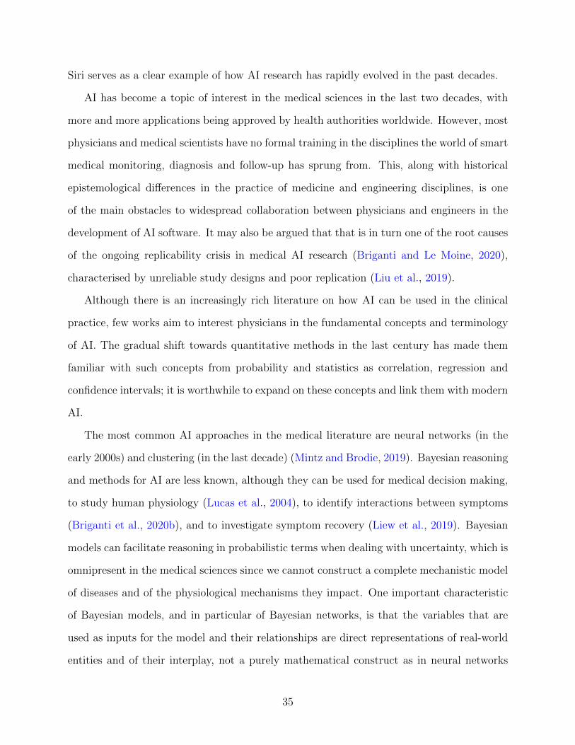
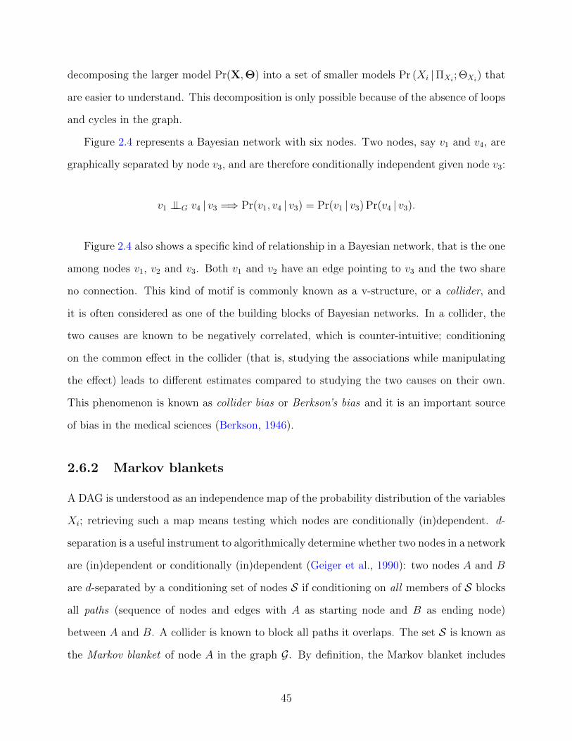
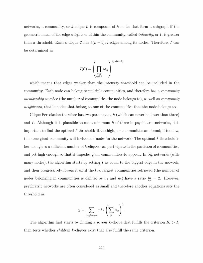
Figure 2.3: A Bayesian network, or Directed Acyclic Graph composed of seven depressionsymptoms from the Zung Depression Scale. Edges are directed from one node to anothernode.

Gaussian, conditional linear Gaussian (Scutari and Denis, 2015). Discrete Bayesian networks

have, for instance, been used in expert systems to differentiate between tuberculosis and

lung cancer (Lauritzen and Spiegelhalter, 1988). Gaussian Bayesian networks are common

is genetics and systems biology for reconstructing direct and indirect gene effects (Kruijer

et al., 2020), and together with conditional Gaussian Bayesian networks they have been used

to study various clinical treatments and conditions (Liew et al., 2019; Dao et al., 2016).

An example of Bayesian networks: psychiatric symptoms

Bayesian networks have been used to investigate causal relationships among psychiatric

symptoms, such as depression symptoms (Briganti et al., 2020b): an example of Bayesian

networks composed of seven depression symptoms from the Zung Depression Scale (Zung,

1965) is represented in figure 2.3.

42

Such Bayesian networks are computed from a data set of symptom scores: edges there-

fore represent admissible causal relationships among symptoms (Moffa et al., 2017). In the

example shown in figure 2.3, for instance, depressive mood has a causal relationship directed

towards weight loss, which in turn has a causal relationship directed towards irritability.

2.5 Difference between neural networks and Bayesian

networks

Neural networks, often called Artificial Neural Networks (ANNs), are in widespread use

in the AI field. They represent networks of interconnected artificial neurons that change

their state with the external or internal information that flows through the network during

a learning phase (Hecht-Nielsen, 1990). Neural networks are usually organised in several

layers: an input layer, several intermediate layers of latent variables, and an output layer.

Their aim is to identify a relationship between the input and the output. Hence they are

discriminative models, and do not provide any insight into the interplay of the variables nor

a semantic representation of causes and effects. They are known to be difficult to interpret

(Correa et al., 2009), to the point that post hoc methods to improve their interpretability

and explainability are now a challenging new avenue for research(Holzinger et al., 2019). The

key advantage of Bayesian networks is that they model of the real world: the phenomenon

under investigation is understood by the machine, dissected, and clearly represented as a

set of causal relationships. This allows for a predictive reasoning much needed in medicine:

Bayesian networks can answer diagnostic and prognostic questions of the form “how will

symptom/sign/disease A change if we act upon symptom/sign/disease B?” in a way that is

understandable by both patients and clinicians. This is possible because of the reversibility

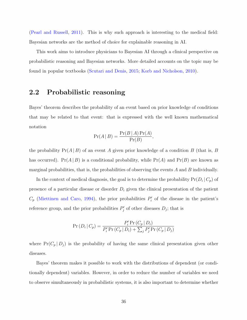
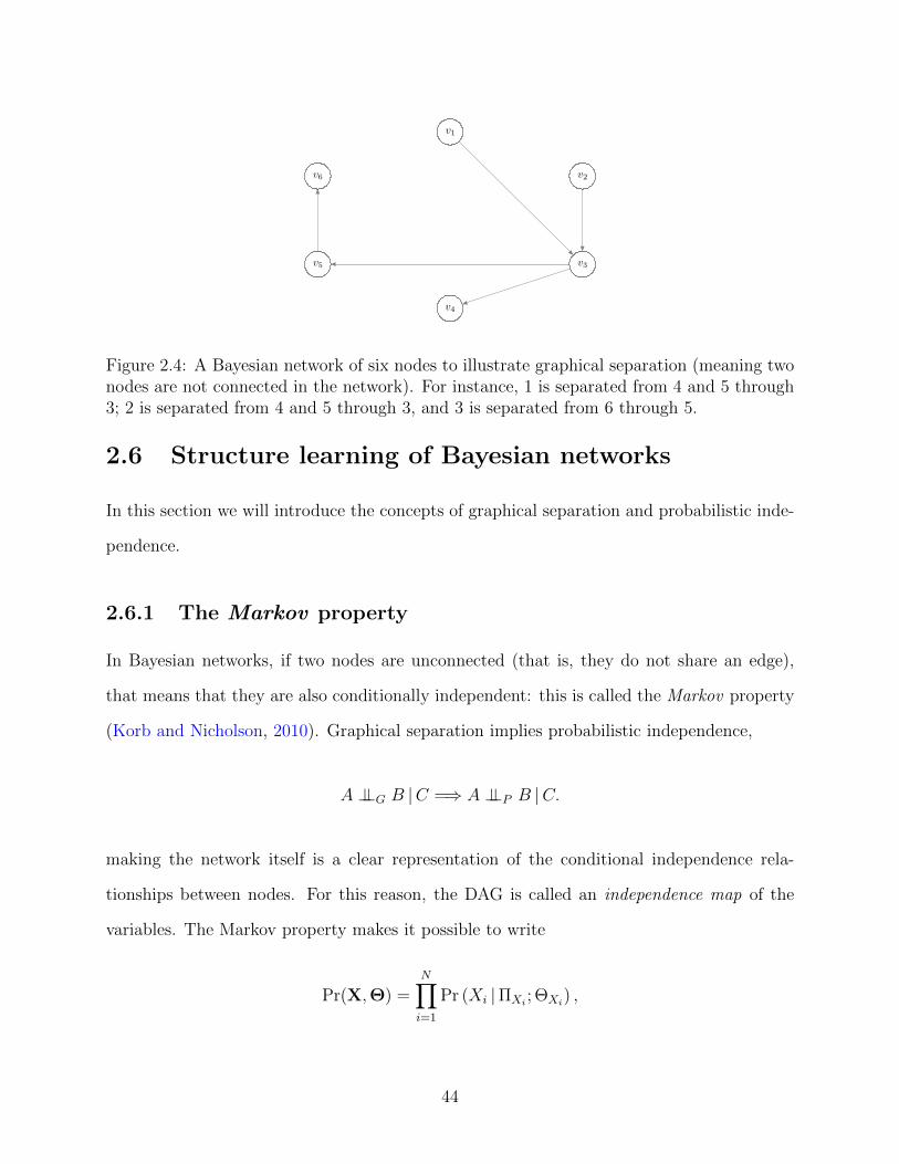
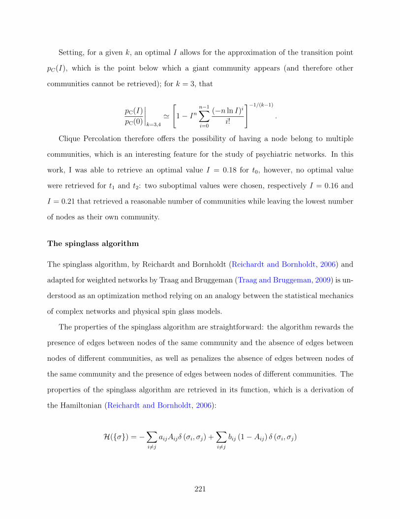
of Bayes’ theorem (Pr(A |B) Pr(B) = Pr(A,B) = Pr(B |A) Pr(A)).

43

Figure 2.4: A Bayesian network of six nodes to illustrate graphical separation (meaning twonodes are not connected in the network). For instance, 1 is separated from 4 and 5 through3; 2 is separated from 4 and 5 through 3, and 3 is separated from 6 through 5.

2.6 Structure learning of Bayesian networks

In this section we will introduce the concepts of graphical separation and probabilistic inde-

pendence.

2.6.1 The Markov property

In Bayesian networks, if two nodes are unconnected (that is, they do not share an edge),

that means that they are also conditionally independent: this is called the Markov property

(Korb and Nicholson, 2010). Graphical separation implies probabilistic independence,

A ⊥⊥G B |C =⇒ A ⊥⊥P B |C.

making the network itself is a clear representation of the conditional independence rela-

tionships between nodes. For this reason, the DAG is called an independence map of the

variables. The Markov property makes it possible to write

Pr(X,Θ) =N∏i=1

Pr (Xi |ΠXi ; ΘXi) ,

44

decomposing the larger model Pr(X,Θ) into a set of smaller models Pr (Xi |ΠXi ; ΘXi) that

are easier to understand. This decomposition is only possible because of the absence of loops

and cycles in the graph.

Figure 2.4 represents a Bayesian network with six nodes. Two nodes, say v1 and v4, are

graphically separated by node v3, and are therefore conditionally independent given node v3:

v1 ⊥⊥G v4 | v3 =⇒ Pr(v1, v4 | v3) = Pr(v1 | v3) Pr(v4 | v3).

Figure 2.4 also shows a specific kind of relationship in a Bayesian network, that is the one

among nodes v1, v2 and v3. Both v1 and v2 have an edge pointing to v3 and the two share

no connection. This kind of motif is commonly known as a v-structure, or a collider, and

it is often considered as one of the building blocks of Bayesian networks. In a collider, the

two causes are known to be negatively correlated, which is counter-intuitive; conditioning

on the common effect in the collider (that is, studying the associations while manipulating

the effect) leads to different estimates compared to studying the two causes on their own.

This phenomenon is known as collider bias or Berkson’s bias and it is an important source

of bias in the medical sciences (Berkson, 1946).

2.6.2 Markov blankets

A DAG is understood as an independence map of the probability distribution of the variables

Xi; retrieving such a map means testing which nodes are conditionally (in)dependent. d-

separation is a useful instrument to algorithmically determine whether two nodes in a network

are (in)dependent or conditionally (in)dependent (Geiger et al., 1990): two nodes A and B

are d-separated by a conditioning set of nodes S if conditioning on all members of S blocks

all paths (sequence of nodes and edges with A as starting node and B as ending node)

between A and B. A collider is known to block all paths it overlaps. The set S is known as

the Markov blanket of node A in the graph G. By definition, the Markov blanket includes

45

a node’s parents (nodes with an edge directed towards A), children (nodes that receive a

directed edge from A), and spouses, that is, children’s other parents. The Markov blanket

is useful in investigating a target node of interest while forgetting about the rest of the

Bayesian network; all nodes outside of the Markov blanket are independent from the node

of interest.

2.6.3 Bayesian networks and Causality

Since Bayesian networks are based on DAGs, the relationships among variables are easily

interpreted as causal relationship. However, three assumptions should be made before inter-

preting an edge as a causal effect. First, each variable (node) must conditionally independent

of its indirect and direct non-effects given its direct causes (this is the causal translation of

the Markov property). Second, there must exist a DAG faithful to the probability distribu-

tion of X so that the only dependencies in the probability distribution are those that arise

from d-separations in the DAG. The third assumption descends from the first two: there

must be no latent variables that act as confounding factors (therefore developing causal ef-

fects on one or several nodes in the network without the DAG reporting such relationships).

The third assumption is particularly important in clinical settings: to safely interpret a di-

rected connection as a causal effect, the experimental design should be set as to block any

confounding factors. A common device to achieve that is randomisation, which severs any

incoming causal link between the randomised variables and possible exogenous effects.

It is important to make a distinction between the probabilistic and causal interpretations

of Bayesian networks. From a causal perspective, the direction of arcs is uniquely identified

by the asymmetry between cause and effect: if we act on the cause, we may influence

the effect; but if we act on the effect, the cause remains unaffected. From a probabilistic

perspective, this is not true because of the reversibility of Bayes’ theorem. For instance, if

46

we consider again the DAG in Figure 2.2 we can write

Pr(v1, v2, v3, v4, v5) = Pr(v1) Pr(v2 | v1) Pr(v3 | v2) Pr(v4 | v2, v3) Pr(v5 | v2, v4)

where each node has a distribution conditional on its parents. However, for the nodes v1 and

v2 we have that Pr(v1) Pr(v2 | v1) = Pr(v2) Pr(v1 | v2). This implies that the DAG in which

the arc v1→ v2 is reversed into v2→ v1 encodes the same probability distribution as that in

Figure 2.2, despite having different arcs. The only arcs whose direction cannot be changed

in this way, and is thus uniquely identified even without making causal assumptions, are

those that are part of a collider; or those that would be part of a new collider or introduce

a cycle if they were reversed.

Another consequence of the duality between the probabilistic and the causal interpreta-

tion of Bayesian networks is that we can compute the conditional probability of any pair

of variables regardless of how we construct the DAG. Depending on the application, it may

make more sense to use a prognostic DAG in which arcs point from diseases to symptoms,

or a diagnostic DAG in which arcs point from symptoms to diseases. From a purely proba-

bilistic perspective, we note that for every diagnostic DAG there is a prognostic DAG that

represents the same probability distribution and vice versa. Clearly, one will be easier to

interpret than the other because the DAG will be easier to read. However, any conditional

probability we may wish to compute will be identical for both.

2.6.4 Structure learning algorithms

Structure learning algorithms learn the structure of Bayesian networks from data, given the

assumptions of Bayesian networks (such as the Markov property). Constraint-based algo-

rithms use statistical tests to learn conditional independence relationships (the constraints

themselves); score-based algorithms rank candidate DAGs based on some goodness-of-fit

criterion; hybrid algorithms use conditional independence tests to exclude the vast majority

47

of candidate DAGs, and then perform a score-based search on the few that are still under

consideration.

The Inductive Causation algorithm and its implementation

The Inductive Causation algorithm (IC) (Pearl and Verma, 1995) is the simplest example of

structure learning constraint-based algorithm.

Firstly, for each pair of variables A and B in X, the algorithm searches for a set SAB

such that A and B are independent given SAB and such that A and B are not part of it

(A,B /∈ SAB). Secondly, for each pair of variables that are not connected by an edge but that

are both connected to a common neighbour C, the algorithm checks whether C ∈ SAB: if

C /∈ SAB, then the direction of edge A−−C becomes A→C and that of edge C −−B becomes

C←B. Thirdly, the direction of the edges that are still undirected is set following two rules:

if A is adjacent to B and there is a strictly directed path from a to B, then A−−B becomes

A→B; if A and B are not adjacent but A→C and C −−B, then C −−B becomes C→B.

This step ends the algorithm which then returns the partially directed graph in which only

those arc directions that can be uniquely identified from the data are represented. The IC

algorithm is implemented by the Peter & Clark algorithm (PC) (Spirtes et al., 1993), which

starts from a saturated network and then performs tests that gradually increases the number

of conditioning nodes.

2.7 Discussion: applications and limitations of Bayesian

Artificial Intelligence in Medicine

Bayesian AI and networks are in use in several areas in the medical science and are a tool

of interest for physicians.

Applications of Bayesian AI in medicine stem from four main domains: diagnostic

reasoning—establishing a diagnosis in a target patient given clinical evidence; prognostic

48

reasoning—making predictions about what might happen in the future, since Bayesian net-

works encode a temporal information even in cross-sectional data; treatment selection—

making predictions about the possible effects for a treatment; studying functional interac-

tions among clinical evidence such as symptoms, signs and biomarkers.

Several examples from the four main domains described above illustrate the vast poten-

tial of Bayesian AI. First, recovering clinical evidence from the electronic medical record

is a substantial starting block for making inference: systems to construct clinical Bayesian

networks from electronic medical records have been developed (Shen et al., 2018). Second,

prognostic Bayesian networks are used to predict mortality in patients (Verduijn et al., 2007).

Third, Bayesian networks are also used for clinical decision support and treatment selection

in complicated cases (Sesen et al., 2013). Fourth, studying functional interactions among

symptoms in the medical domain of psychiatry shows great promise: because the classifica-

tion of mental disorders is rapidly shifting paradigms, the new approach of mental disorders

as networks of mutually influencing components (Borsboom and Cramer, 2013) is a promis-

ing setting for the application of Bayesian reasoning. Works have already endeavoured to

represent interacting symptoms for disorders like depression as DAGs in cross-sectional data,

therefore retrieving the possible causal relationships among them (Briganti et al., 2020b).

Future work in this area may for instance include different types of variables (other than

symptoms) in networks.

The use of Bayesian networks is limited by the assumptions required to correctly learn and

perform inference on their structure. It is up to the researchers to design studies accordingly:

blocking confounding variables is by far the most difficult task in this respect (Briganti et al.,

2020b).

In conclusion, Bayesian artificial intelligence captures uncertain reasoning in medicine

through the promising model of Bayesian networks: they can be learned automatically from

data and combine graphs and probabilities in a rigorous way, with algorithms that automate

reasoning and use the graphical part of the model to guide a computer system in computing

49

probabilities and predict events of interest.

50

Chapter 3

A primer on undirected network

models

Abstract

In this work the estimation, inference and stability of network models with undi-

rected edges for the study of mental disorders are reviewed. Gaussian Graphical Models

and Ising Models capture the statistical relationships among variables of interest such

as symptoms in a network of mutually influencing items in continuous and binary data

sets. Cross-sectional networks as well as temporal networks can be estimated. The

main measures of inference in such networks, such as centrality, as well as the impor-

tance of stability analyses are also reviewed. The clinical implications of the study of

mental disorders as networks are discussed.

3.1 Introduction

The network theory of mental disorders considers that the psychiatric disease arises from

the set of interactions among its symptoms (Borsboom, 2008). Network theory comes with

a specific set of statistics called network analysis which includes methods allowing for the

study of network models from data sets (Epskamp and Fried, 2018).

51

Several steps are necessary when studying mental disorders as network structures. First

the network structure itself must be estimated from the data set: this first step implies a

choice for the network model itself, which can be estimated from continuous data set through

a Gaussian Graphical Model (GGM), or from a binary data set through an Ising Model

(IM), with or without a regularization procedure (Epskamp, 2019). Second, the relative

or absolute importance, or centrality of a network component, such as a symptom, can be

inferred from the network structure through several measures, such as strength, expected

influence, or bridge centrality. Third, the stability of the parameters that are estimated

within the network structure is evaluated through bootstrapping analyses (Epskamp and

Fried, 2018).

This work aims to review the fundamental concepts introduced in the emerging field of

network analysis: first, the GGM and its binary counterpart, the IM in cross-sectional data-

sets with both frequentist and Bayesian methods; second, the GGM in temporal (panel) data

sets; third, the most common inference techniques; third, the main stability analyses. The

clinical implications of the models are also discussed throughout this work.

3.2 Estimating network models from cross-sectional data

3.2.1 Network components in undirected graphical models

A node is defined as an entity, such as a part of a psychiatric construct or a symptom

(Briganti et al., 2018). An edge (a connection between two nodes) is understood as a pairwise

association between two variables. The network G = (V,A) is therefore composed of a set of

nodes V = {v1, v2, . . . , vp} and a set of edges A. In undirected graphical models, the edges

are weighted, that is, some edges are stronger than others in the network structures.

52

3.2.2 The Gaussian Graphical Model

Let y be a a normal multivariate vector y = (y1, ..., yp) with mean vector µ and a variance-

covariance matrix Σ. For all subjects,

y ∼ N(µ,Σ).

Let Θ be the inverse of Σ,

Θ = Σ−1

that is known as the precision matrix or a Gaussian Graphical Model (GGM). The

elements of of the GGM encode the partial correlation coefficients θij of two variables yi and

yj given all other variables in y, that is, y−(i,j):

Cor(yi, yj|y−(i,j)

)= − θij√

θii√θjj,

therefore, the GGM represents the network itself.

The partial correlation θij between yi and yj is used as the edge weight, that is, the

strength of the connections between nodes vi and vj in the network. Edge weights can be

positive (usually represented as blue connections) or negative (usually represented as red

connections) depending on the sign of θij. The presence of an edge between two nodes vi

and vj in the network can be interpreted as a conditional dependence relationship: node

Vi predicts (or is predicted by) node vj, after controlling for all other nodes in the network

v−(ij). GGMs can be estimated in R with the bootnet package (Epskamp and Fried, 2018).

3.2.3 Bayesian estimation of the Gaussian Graphical Model

The estimation of a GGM with Bayesian methods allows for providing evidence for the

hypothesis that best predicts the observed data. For instance, when testing for conditional

53

dependence relationships among nodes, providing a Bayes Factor between 3 and 20 as a

cut-off value is associated with positive evidence, while a Bayes Factor > 20 is associated

with strong evidence (Kass and Raftery, 1995). In this section an overview is provided to

Bayes Factor and the Wishart distribution, both necessary for the estimation of a Bayesian

GGM. They can be computed in R with the BGGM package (Williams and Mulder, 2019).

Bayes Factor

Bayes factor is used for the selection of a statistical model by quantifying the support for

a model over another (Lambert, 2018): it is understood as the radio of the conditional

probabilities of the data given the first model and the second model

Bf =p (data | model1)

p (data | model2),

that is, the ratio of the marginal likelihoods for each model p(data | modeli). Given a

variable X = (x1, x2, . . . , xp) with a probability distribution of parameters Θ, the marginal

likelihood is the probability p(X | model) where Θ has been integrated out (marginalized

out).

p(X | model) =

∫Θ

p(X | Θ)p(Θ | model)dΘ

Bayes factor chooses more parsimonious models and therefore penalizes complexity.

Wishart distribution

Given the multivariate data set with a normal distribution with mean 0, X ∼ (0,Σ), an

m× p matrix of , subjects and p variables X = (x1, x2, . . . , xp), the Wishart distribution

Wprior ∼ (Q, h)

is the conjugate prior (that is, the prior probability distribution) of the inverse-covariance

54

matrix or precision matrix, where Q is the scale matrix and h the degrees of freedom such

as h > p− 1. The posterior distribution is also a Wishart distribution

Θ | X ∼ Wposterior

(h+ n, (Sq + εIp)

−1)where Ip is the identity matrix, and Sq the sums of squares matrix X ′X. (Williams,

2018b). The Wishart probability distribution function follows

fΘ(θ) =|θ|(n−p−1)/2e− tr(Q−1θ)/2

2np2 |Q|n/2Γp

(n2

)where Γp is the multivariate gamma function (generalization of the factorial function for

complex numbers in multivariate statistics), and tr is the trace function (the sum of elements

on the main diagonal) of the square matrix.

3.2.4 The Ising Model

The Ising Model (IM) is the binary equivalent of the Gaussian Graphical Model (van Borkulo

et al., 2014; Marsman et al., 2018) used to estimate a network of partial correlations in

continuous datasets. From an Ising Model perspective, each variable in the network is

influences by all other variables, and this is represented in the following distribution for a

given variable X:

Z =∑x

exp

(∑i

τixi +∑<ij>

ωijxixj

).

With the Ising Model it is possible to determine the conditional probability distribution

of a variable Xi as it is predicted by other variables in the network given that their values

are known X(−i),

55

Pr(Xi|X(−i) = x(−i)

)=

Pr(X = x)

Pr(X(−i) = x(−i)

) =exp

(xi

(τi +

∑j ωijxj

))∑

xiexp

(xi

(τk +

∑j ωijxj

))where τ represents the threshold parameter which determines whether the variable Xi

prefers to be in state +1 (if τ is higher than 0) or -1 (if τ is lower than 0), ωij represents

the pairwise interaction between two variables Xi and Xj, and∑

xitakes the sum over both

possible outcomes of xi, that is the logistic regression model. Neural networks are used to

fit a non-regularized multinomial logistic regression as a loglinear binary logistic regression

in the data set (Venables and Ripley, 2002).

This is achieved by modeling the logarithm of the probability of seeing a given output

for the predicted variable Xi using the linear predictor X(−i) (that is, all other variables in

the network) and a normalization factor, the logarithm of the partition function:

ln Pr (Xi = K) = βK ·X(−i) − lnZ

where K is the given output, βK the regression coefficient and lnZ is the logarithm of

the partition function, which in turn can be estimated as

Z =K∑k=1

exp(βk ·X(−i))

,

and represents a constant, in terms that it does not depend on the predicted variable

Xi. The partition function, compared to the Ising distribution, generates the following

equivalency for the linear predictor

∑i

τixi +∑<ij>

ωijxixj = βK ·X(−i)

in the multinomial logistic regression approach to the Ising Model.

56

Because of the need to sum many terms to estimate the Ising Model, the computation

without using additional techniques is only possible for data sets where the number of vari-

ables is inferior or equal to 10. Regularized versions of the Ising Model, such as used in

recent applied studies (Briganti and Linkowski, 2019a) allow for computation in data sets

with a higher number of variables. Ising Models can be computed in R with the bootnet

package (Epskamp and Fried, 2018).

3.2.5 Interpreting undirected network models in cross-sectional

data sets

The interpretation of the network model depends on the model itself and the variables in-

cluded. The interpretation of a connection in a network is somewhat more straightforward

for symptoms: if symptom A and symptom B are connected in a network, than the two pre-

dict each other. It is less straightforward however to interpret connections among two items

from a psychometric scale that measures a construct: one can interpret that a connection

still means that the traits that are measured predict each other, and its clinical implication

lies in the better understanding of psychiatric constructs themselves.

3.3 Estimating network models from several time points

Panel data are interesting to monitor the evolution of symptoms over time, for instance on

admittance, at the middle and the end of the hospital stay of a patient. To see whether

a symptom at one time point influences another symptom at the subsequent time point, a

specific network model exists that allow for the encoding of temporal effects. Such temporal

predictions are known as Granger causality. In this section, both Granger causality and the

temporal network models are reviewed.

57

3.3.1 Granger causality

Granger causality is a statistical test (Granger, 1969) for the hypothesis that a variable (or

a set of variables) predicts another (Lutkepohl, 2005).

Let X(t) ∈ Rd×1 for t = 1, . . . , T be a d-dimensional panel data set. Granger causality is

obtained by estimating a Vector Auto-Regressive (VAR) model with L time lags

X(t) =L∑τ=1

AτX(t− τ) + ε(t)

where τ = 1, . . . , L, ε(t) a Gaussian random vector, and Aτ a matrix for every τ . A

variable Xi is said to Granger-cause another variable Xj if the element Aτ (ji) is greater

than 0.

3.3.2 The Graphical Vector Autoregressive Model

To model the dynamics of manic symptoms with a pharmacological intervention in panel

data, a panel Graphical Vector Autoregressive Model (GVAR). This model was first intro-

duced in recent works with its own package for computation (Epskamp, 2019) to translate

time-series methods to panel data. GVAR can be seen as a multivariate multiple regression

on the previous measurement occasion.

For a set of symptoms y = (y1, ..., yp) measured in a given individual, GVAR is expressed

as

yt1 |yt0 ∼ N(µ+B(yt0 − µ),Σζt0),

where B represents a p × p matrix of temporal effects, µ the vector of means, Σt0 the

variance-covariance matrix on measurement occasion t0, and ζ a vector of normally dis-

tributed innovations. Because B encodes temporal prediction, a nonzero matrix element bij

means that yt1 is predicted by yt0 : this prediction is known as Granger causality (Granger,

1969) because the condition of cause preceding the effect is fulfilled.

58

3.4 Network inference

Network inference is the domain of network analysis that deals with reaching conclusions

about the network structure that has been estimated from the data. Often, network re-

searchers want to study which nodes are more important than others: in psychiatry, that

translates with identifying symptoms that could be chosen as targets for a clinical interven-

tion (either with psychopharmacology or with psychotherapy).

3.4.1 Centrality

Network centrality is a relative approach to identifying important symptoms or items in a

network: it is relative because there will always be a more central item, even in a poorly

connected network (Briganti et al., 2019). Network centrality is however important in identi-

fying which symptoms connect more than others, and can therefore aid in poorly connected

networks.

Strength (sometimes called degree) is the absolute sum of the edge weights w of a node

Vi,

CwS (i) =

N∑j

| wij |

A variant of strength is expected influence (Jones, 2017), which is the sum of edge weights,

and therefore accounts for negative edges in a network

CwEI(i) =

N∑j

wij.

Betweenness is understood as the shortest paths that go through the node under investi-

gation, while closeness measures the sum of shortest paths from the node under investigation

to all other nodes in the network (Boccaletti et al., 2006); betweenness and closeness are

seldom used in symptom networks.

59

3.4.2 Node predictability

Node predictability is used to have an absolute estimate of a node’s connectedness: the

measure of R2 (coefficient of determination) is used to convey this information.

Let us consider a regression model of outcomes y and predictors X with predicted values

E(y | X, θ), fit to data (X, y)n, n = 1, . . . , N. Ordinary least squares yields an estimated

parameter vector θ with predicted values yn = E(y | Xn, θ

)and residual variance VarNn=1 yn,

where I am using the notation,

VarNn=1 zn =1

N − 1

N∑n=1

(zn − z)2 , for any vector z

Node predictability, that is, the proportion of shared variance, is

R2 =VarNn=1 yn

VarNn=1 yn

and is computed as an R function in the package mgm (Haslbeck and Waldorp, 2016).

A Bayesian approach to the estimation of node predictability also exists as it was in-

troduced recently in the literature (Gelman et al., 2019). Expected values conditional on

unknown parameters are used

ypredn = E (yn | Xn, θ)

where yn represents a future observation from the model with predictors Xn. However,

because several posterior distributions are drawn θs, s = 1, . . . , S the vector of predicted

values is written as ypredsn = E (y | Xn, θ

s).

The residual variance varres is defined as

varres = E(V Nn=1

(yn − ypred

n

)| θ)

60

and the Bayesian R2 is expressed as

Bayesian R2s =

VarNn=1 ypred sn

VarNn=1 ypred sn + varsres

,

and is computed as a function in the R package BGGM (Williams and Mulder, 2019).

Although it is interpreted as an absolute measure of connectedness, it is also understood

as the upper bound of controllability : if one assumes that all the edges of a node are directed

towards it, then node predictability reflects how a node can be controlled; on the other hand,

if one assumes that all the edges are directed towards other nodes, than node predictability

reflects how a node can control others (Briganti et al., 2019).

3.5 Stability and accuracy

The question of stability and accuracy of results obtained in the estimation of psychiatric

networks quickly became important in this new field of research. Networks have shown

similar results in several populations in the context of post-traumatic stress disorder (Fried

et al., 2018) and this adds a supporting argument for the replication of the results obtained

via these analyzes.

The most used instrument to analyze the stability and precision of network parameters

is bootstrapping (Epskamp and Fried, 2018). This method re-calculates the parameters that

make up the network to answer specific questions. As far as the edges are concerned, the

two questions are as follows: 1) is edge A between two nodes X and Y really larger than

edge B between two nodes V and W? and 2) is edge A accurately estimated?

To answer the first question, confidence intervals are estimated around the difference

between edges A and B as determined by a number of re-estimates of choice; generally, 2000

network re-estimates are performed (Briganti et al., 2018), if this test proves positive, the

observer can interpret that an edge A is significantly larger than an edge B (Briganti et al.,

2019). To answer the second question, confidence intervals are calculated around several

61

thousand re-estimates from all edges of the network. If these confidence intervals are not

very wide and do not overlap between different edges, then the observer can better appreciate

the difference between different edges of the network.

The same process can be applied for centrality indicators: in that case, subset bootstrap-

ping is applied, that is, a bootstrapping process that involves gradually reducing the number

of subjects in the sample and re-estimating the network parameters so as to test how stable

is the centrality order (the order of which symptoms rank in centrality estimates).

3.6 Conclusion

This work aimed to review the introductory concepts of network analysis of undirected graph

structures and how to conduct such analyses in cross-sectional and time-series. Although

specific to the field of networks of mental disorders, these statistical techniques can be applied

in a wide range of specialties and are highly versatile for both low and high dimensional data.

62

Part II

A network approach to mental

constructs

63

Chapter 4

A network model of empathy

Abstract

The aim of this work is to perform a network analysis on the French adaptation

of the Interpersonal Reactivity Index (IRI) scale from a large Belgian database and

provide additional information for the construct of empathy. I analyze a database of

1973 healthy young adults who were queried on the IRI scale. A regularized partial

correlation network is estimated. In the visualization of the model, items are displayed

as nodes, edges represent regularized partial correlations between the nodes. Central-

ity denotes a node’s connectedness with other nodes in the network. The spinglass

algorithm and the walktrap algorithm are used to identify communities of items, and

state-of-the-art stability analyses are carried out. The spinglass algorithm identifies

four communities, the walktrap algorithm five communities. Positive edges are found

among nodes belonging to the same community as well as among nodes belonging to

different communities. Item 14 (“Other people’s misfortunes do not usually disturb

me a great deal”) shows the highest strength centrality score. The network edges and

node centrality order are accurately estimated. Network analysis highlights interesting

connections between indicators of empathy; how these results impact empathy models

must be assessed in further studies.

64

4.1 Introduction

Empathy is a main component of short-term as well as long-term human interactions. Despite

its importance and because of its complexity, a unified definition is yet to be found. For some

authors, empathy incarnates the ability to perceive and be sensitive to others’ emotions and

the desire for their well-being (Decety et al., 2016). It is not to be confused with sympathy,

which is considered to be a part of empathy and defined as the consciousness of another’s

emotions and feelings without sharing them, together with a feeling of pity (Wispe, 1986).

Empathy is a key item to mental health professionals because it belongs to a collection of

indicators of good outcomes in psychotherapy (Elliott et al., 2011).

In 1980, Mark H. Davis presented a self-report empathy questionnaire, the Interpersonal

Reactivity Index (IRI), where he identified the construct as built upon two dimensions (Davis,

1980). The first one represents the cognitive dimension, or the tendency to adopt others’

perspectives and feelings; the second one represents an affective dimension reflecting one’s

feeling of another’s emotional state (Decety and Jackson, 2004).

Out of these two dimensions Davis identified four components in his model of empathy:

(1) Fantasy (belonging to the cognitive dimension), or the tendency to get involved in the

actions and feelings of one or more fictional characters in movies, books or plays (e.g.,

item 23—“When I watch a good movie, I can very easily put myself in the place of a

leading character”); (2) Perspective taking (also belonging to the cognitive dimension), or

the tendency to comprehend others’ point of view (e.g., item 25—“When I am upset at

someone, I try to put myself in his shoes for a while”); (3) Empathic concern (belonging

to the affective dimension), the feeling of concern and sympathy for people in distress (e.g.,

item 9—“When I see someone being taken advantage of, I feel kind of protective toward

them”); (4) Personal distress (also belonging to the affective dimension), or the feeling of

unease in difficult, tense or emotional situations (e.g., item 10—“I sometimes feel helpless

when I am in the middle of a very emotional situation”).

Even though the two-dimension model is frequently accepted (Bohart and Greenberg,

65

1997; Davis, 1980; Decety and Jackson, 2004; Reniers et al., 2011), further models were pro-

posed, such as Blair’s (Blair, 2005), which distinguished three components (motor, cognitive

empathy and emotional). Cliffordson proposed a hierarchical model putting the empathic

concern factor at the top of the pyramid (Cliffordson, 2002). Empathy is an important issue

for psychiatrists. Its dysfunctioning is part of major psychiatric diseases such as psychopathy

and autism (Blair, 2005) and is perceived by patients as a key element to treatment (Ross

and Watling, 2017).

In the last few years, a new way of analyzing data in psychology and psychiatry has

arisen: network analysis. In this conceptual model (Borsboom and Cramer, 2013), pairwise

interactions among symptoms represent a network of mutually influencing elements. This

model has affirmed itself as a way of analyzing mental disorders such as depression (Beard

et al., 2016; Boschloo et al., 2016; Fried and Cramer, 2017), posttraumatic stress disorder

(Bryant et al., 2017), as well as autism and obsessive–compulsive disorder (Ruzzano et al.,

2015) by focusing on the interaction between symptoms, attributes, emotions, and behaviors

(Fried and Cramer, 2017).

Network analysis provides a new opportunity to conceive psychological constructs not as

the consequence of an underlying disease as in the latent variable model, but instead as con-

stituted by the mutual interaction of its items. While largely applied to research on mental

illness, network models have been used in other psychological sciences such as personality

(Costantini et al., 2015), health-related quality of life (Kossakowski et al., 2016), intelligence

(van der Maas et al., 2006), and attitudes (Dalege et al., 2017). Network models have also

been used to specifically investigate the structure of multivariate data in psychology, for

instance to identify the number of item clusters: this is the case of recent papers concerning

PTSD (Gluck et al., 2017) and development (Demetriou et al., 2017).

This paper extends this conceptual framework to the psychological construct of empathy.

Network analysis facilitates the identification of interactions between psychological variables

such as items on self-report questionnaires; allows for the estimation of item communities

66

(i.e. clusters of items that are closely related with each other); and can give insights into the

connectedness or importance of items within the network, often referred to as ‘centrality’

(Boccaletti et al., 2006).

According to Davis’ model (1980), I might expect significant positive relations between

items from the Empathic concern scale and items from the Perspective taking and the Fan-

tasy scales. Inspired by network analysis in other fields of psychological science, I apply

network models for the first time to the domain of empathy research, specifically, to the 28-

item French version of the IRI (Braun et al., 2015). This paper highlights potential insights

that network analysis can offer — as a complementary tool to factor modeling that is more

established in the field — to empathy research. The primary aim of the paper is to explore

empathy items and their relationships in an empathy network, and the secondary aim is to

build up on prior factor modeling work in this dataset. Braun and colleagues used confir-

matory or exploratory factor analysis (CFA and EFA) to investigate the factor structure in

the present data (Braun et al., 2015), and I want to use community detection algorithms to

see whether the results align with prior work, and to discuss why the identified communities

have a radically different interpretation (Demetriou et al., 2017; Golino and Epskamp, 2017).

4.2 Method

4.2.1 Data set

The database for this study was composed of 1973 French-speaking students in several uni-

versities or schools for higher education in the following fields: engineering (31%), medicine

(18%), nursing school (16%), economic sciences (15%), physiotherapy, (4%), psychology

(11%), law school (4%) and dietetics (1%). The subjects were 17 to 25 years old (M = 19.6

years, SD = 1.6 years), 57% were females and 43% were males. Even though the full data set

was composed of 1973 participants, only 1270 answered the full questionnaire: I dealt with

missing data by using pairwise complete observations in estimating a Gaussian Graphical

67

Model, meaning that I used all available information from every subject.

The IRI is composed of 28 items meant to assess the four following components: fan-

tasy, perspective taking, empathic concern and personal distress. In the questionnaire, the

items are mixed; reversed items (items 3, 4, 7, 12, 13, 14, 15, 18, 19) are present. Items

are scored from 0 to 4, where “0” means “Doesn’t describe me very well” and “4” means

“Describes me very well”; reverse-scoring is calculated afterwards. The IRI questionnaires

were anonymized. The reanalysis of the database in this retrospective study was approved

by the ethical committee of the Erasmus Hospital.

Table 4.1: The Interpersonal Reactivity Index.

Item Item Label Domain

color

Item meaning

1 1FS Green I daydream and fantasize, with some regularity, about

things that might happen to me.

2 2EC Purple I often have tender, concerned feelings for people less

fortunate than me.

3 3PT R Yellow I sometimes find it difficult to see things from the “other

guy’s” point of view. (Reversed)

4 4EC R Purple Sometimes I don’t feel very sorry for other people when

they are having problems. (Reversed)

5 5FS Green I really get involved with the feelings of the characters

in a novel.

6 6PD Red In emergency situations, I feel apprehensive and ill-at-

ease.

7 7FS R Green I am usually objective when I watch a movie or play, and

I don’t often get completely caught up in it. (Reversed)

68

8 8PT Yellow I try to look at everybody’s side of a disagreement before

I make a decision.

9 9EC Purple When I see someone being taken advantage of, I feel

kind of protective towards them.

10 10PD Red I sometimes feel helpless when I am in the middle of a

very emotional situation.

11 11PT Yellow I sometimes try to understand my friends better by

imagining how things look from their perspective.

12 12FS R Green Becoming extremely involved in a good book or movie

is somewhat rare for me. (Reversed)

13 13PD R Red When I see someone get hurt, I tend to remain calm.

(Reversed)

14 14EC R Purple Other people’s misfortunes do not usually disturb me a

great deal. (Reversed)

15 15PT R Yellow If I’m sure I’m right about something, I don’t waste

much time listening to other people’s arguments. (Re-

versed)

16 16FS Green After seeing a play or movie, I have felt as though I were

one of the characters.

17 17PD Red Being in a tense emotional situation scares me.

18 18EC R Purple When I see someone being treated unfairly, I sometimes

don’t feel very much pity for them. (Reversed)

19 19PD R Red I am usually pretty effective in dealing with emergencies.

(Reversed)

20 20FS Green I am often quite touched by things that I see happen.

69

21 21PT Yellow I believe that there are two sides to every question and

try to look at them both.

22 22EC Purple I would describe myself as a pretty soft-hearted person.

23 23FS Green When I watch a good movie, I can very easily put myself

in the place of a leading character.

24 24PD Red I tend to lose control during emergencies.

25 25PT Yellow When I’m upset at someone, I usually try to “put myself

in his shoes” for a while.

26 26FS Green When I am reading an interesting story or novel, I imag-

ine how I would feel if the events in the story were hap-

pening to me.

27 27PD Red When I see someone who badly needs help in an emer-

gency, I go to pieces.

28 28PT Yellow Before criticizing somebody, I try to imagine how I

would feel if I were in their place.

4.2.2 Network analysis

The software used for the analysis is R (version 3.4.0, open source, available at https:

//www.r-project.org/). I used the packages qgraph, (Epskamp et al., 2012) and glasso

(Friedman et al., 2014a) for network estimation and visualization, mgm, for node predictabil-

ity (Haslbeck and Waldorp, 2016), igraph, (Csardi and Nepusz, 2006) for the spinglass algo-

rithm, walktrap algorithm and bootnet, (Epskamp and Fried, 2018) for stability.

Network estimation

I estimated Spearman correlations for the 28 ordinal items, which was the input to estimate

a Gaussian Graphical Model (GGM), a regularized partial correlation network (Epskamp

70

https://www.r-project.org/


and Fried, 2018). I used Spearman correlations instead of polychoric correlations because

of low variability between items that can lead to zeroes in the marginal crosstables. The

graphical lasso (least absolute shrinkage and selection operator) was used to regularize the

edge weight parameters resulting from the GGM, which ensures avoiding the estimation of

spurious edges.

Nodes represent items from the French adaptation of IRI. Edges are connections between

two nodes: they are regularized partial correlations between two items of the questionnaire.

An edge between two items therefore means that there is an association after controlling

for all other nodes in the network. Statistically speaking, an edge between items in the IRI

network can be interpreted as following: when two nodes A and B are strongly connected

and the observed group scores high on A, the observed group is more likely to also score

high on B, controlling for all other nodes in the network.

Nodes are placed in the network using the Fruchterman–Reingold algorithm, which de-

termines the position of the node based on the sum of connections it has with other nodes

(Fruchterman and Reingold, 1991). Each edge has a sign: blue edges represent positive

regularized partial correlations whereas red edges represent negative regularized partial cor-

relations. The corresponding thickness and saturation of an edge denote its weight (i.e. the

strength of association).

Network inference

The centrality plot illustrates the centrality of a node in connection with other nodes. Boc-

caletti et al. described three types of centrality: strength, betweenness, and closeness (Boc-

caletti et al., 2006). One can understand strength centrality as the sum of direct connections

a given node has in the network; betweenness is understood as the shortest paths that go

through the node under investigation; closeness measures the sum of shortest paths from the

node under investigation to all other nodes in the network. Since centrality represents the

relative importance of a node in a network, Freeman conceptualized three possible interpre-

71

tations to a central item (Freeman, 1978): control, independence or activity.

Statistically speaking, a central item shares the most variance with all other items. Con-

ceptually, and in case of IRI, which is a self-administered scale, I suggest that the answer of

a subject to a central item might predict the way the subject answers to other items which

share a connection with it in the network. Centrality estimates are standardized with a mean

of 0 and a standard deviation of 1, and strength centrality is the main metric used in this

paper since it is the most robustly estimated centrality metric described in the literature

(Epskamp and Fried, 2018). However, centrality measures are relative metrics, since the

centrality of each node is estimated in comparison with other nodes (there is always a highly

central node, no matter how weak the edges in the network are). I therefore also estimated

node predictability. Node predictability represents the shared variance of each node with

all its neighbors, which constitutes an absolute measure of its interconnectedness (Haslbeck

and Fried, 2017).

The spinglass algorithm was used to identify communities of items in the GGM. It is

based on the principle that edges should connect nodes of the same community, whereas

nodes belonging to different communities should not be connected (Yang et al., 2016). It

is important to note that an item can only be part of one community using this procedure.

Since the spinglass algorithm can give different results in the same sample, I assessed the

stability of the solution by running the algorithm 100 times and extracted the number of

communities with the highest frequency. To complement the results, I also used the walktrap

algorithm, which is based on the principle that adjacent nodes tend to belong to the same

community (Yang et al., 2016). The walktrap algorithm is shown to have high accuracy in

simulation studies (Golino and Epskamp, 2017; Demetriou et al., 2017).

Network accuracy and stability

I tested the accuracy of edge weights and the stability of the order of centrality estimation

through bootstrapping (Epskamp et al., 2017a, I used 2000 bootstraps). I bootstrapped 95%

72

confidence intervals of all edge weights, followed by the edge-weights comparison test and an

edge weight difference test to see which edges differ from each other in size significantly (to

answer the question is edge A significantly larger than edge B). I used the subsetting boot-

strap procedure that re-estimates the network with a dropping percentage of participants to

determine the stability of centrality estimation, and results in a centrality-stability coeffi-

cient (CS-coefficient) that should not be lower than 0.25 and preferably above 0.5. Finally,

I performed a centrality difference test to see which centrality estimates differ statistically

from each other (to answer the question is node A significantly more central than node B).

4.3 Results

4.3.1 Empathy network

Figure 4.1 illustrates the estimated network of the 28-item IRI. Overall, most items are

positively connected within the network. Item 16 (“After seeing a play or movie, I have felt

as though I were one of the characters”) is strongly connected to item 23 (“When I watch a

good movie, I can very easily put myself in the place of a leading character”) (weight 0.38).

Item 4 (“Sometimes I don’t feel very sorry for other people when they are having problems”)

has a wide edge to item 14 (“Other people’s misfortunes do not usually disturb me a great

deal”) (weight 0.29). Other strong edges include item 10 (“I sometimes feel helpless when I

am in the middle of a very emotional situation”) and item 17 (“Being in a tense emotional

situation scares me”), item 24 (“I tend to lose control during emergencies”) and item 27

(“When I see someone who badly needs help in an emergency, I go to pieces”), item 25

(“When I’m upset at someone, I usually try to “put myself in his shoes” for a while”) and

item 28 (“Before criticizing somebody, I try to imagine how I would feel if I were in their

place”).

The spinglass algorithm identifies a mean of four communities of items corresponding to

the four factors of the IRI as proposed originally and confirmed by Braun et al. (Braun

73

1

2

3

4

5

6

7

8

910

11

12

13

14

15

16

17

18

19

2021

22

23

24

25

26

27

28

●

●

●

●

●

●

●

●

●

●

●

●

●

●

●

●

●

●

●

●

●

●

●

●

●

●

●

●

A1: 1FS5: 5FS7: 7FS_R12: 12FS_R16: 16FS23: 23FS26: 26FS

B3: 3PT_R8: 8PT11: 11PT15: 15PT_R21: 21PT25: 25PT28: 28PT

C2: 2EC4: 4EC_R9: 9EC14: 14EC_R18: 18EC_R20: 20EC22: 22EC

D6: 6PD10: 10PD13: 13PD_R17: 17PD19: 19PD_R24: 24PD27: 27PD

●

●

●

●

●

●

●

●

●

●

●

●

●

●

●

●

●

●

●

●

●

●

●

●

●

●

●

●

A1: 1FS5: 5FS7: 7FS_R12: 12FS_R16: 16FS23: 23FS26: 26FS

B3: 3PT_R8: 8PT11: 11PT15: 15PT_R21: 21PT25: 25PT28: 28PT

C2: 2EC4: 4EC_R9: 9EC14: 14EC_R18: 18EC_R20: 20EC22: 22EC

D6: 6PD10: 10PD13: 13PD_R17: 17PD19: 19PD_R24: 24PD27: 27PD

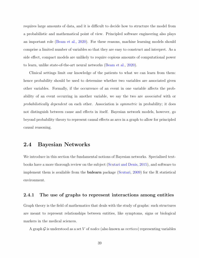
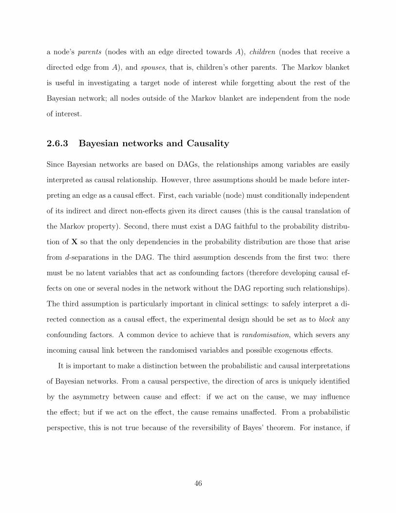
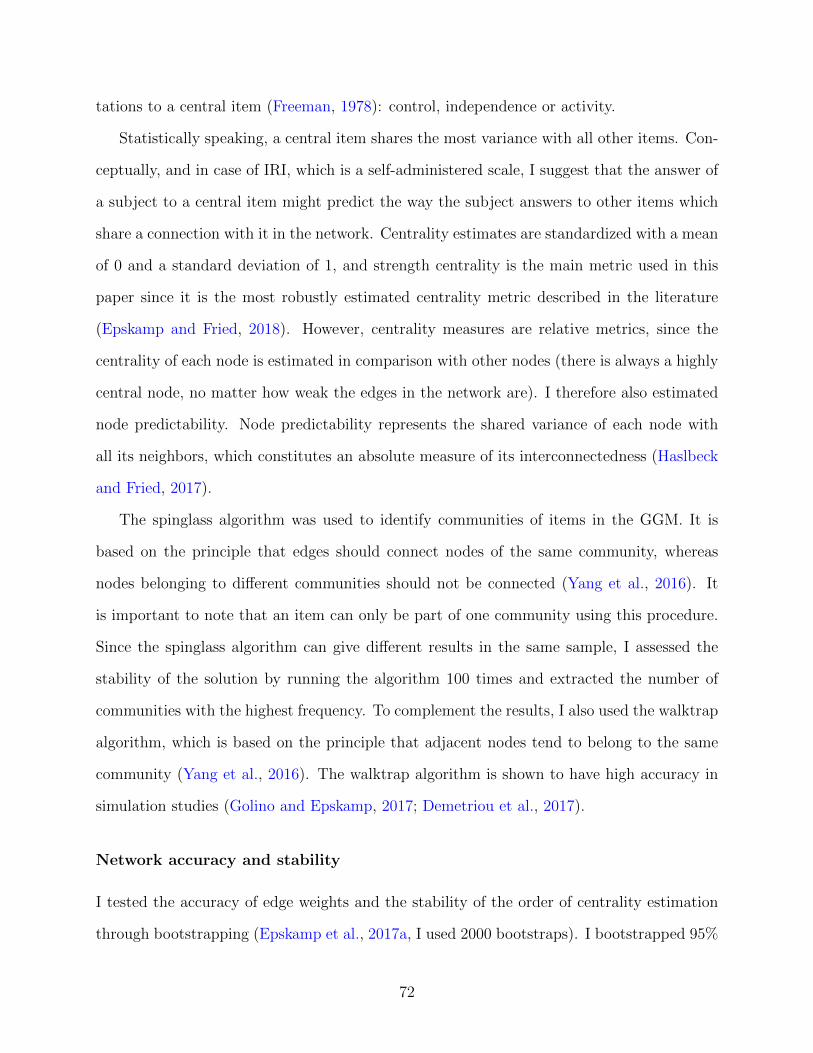
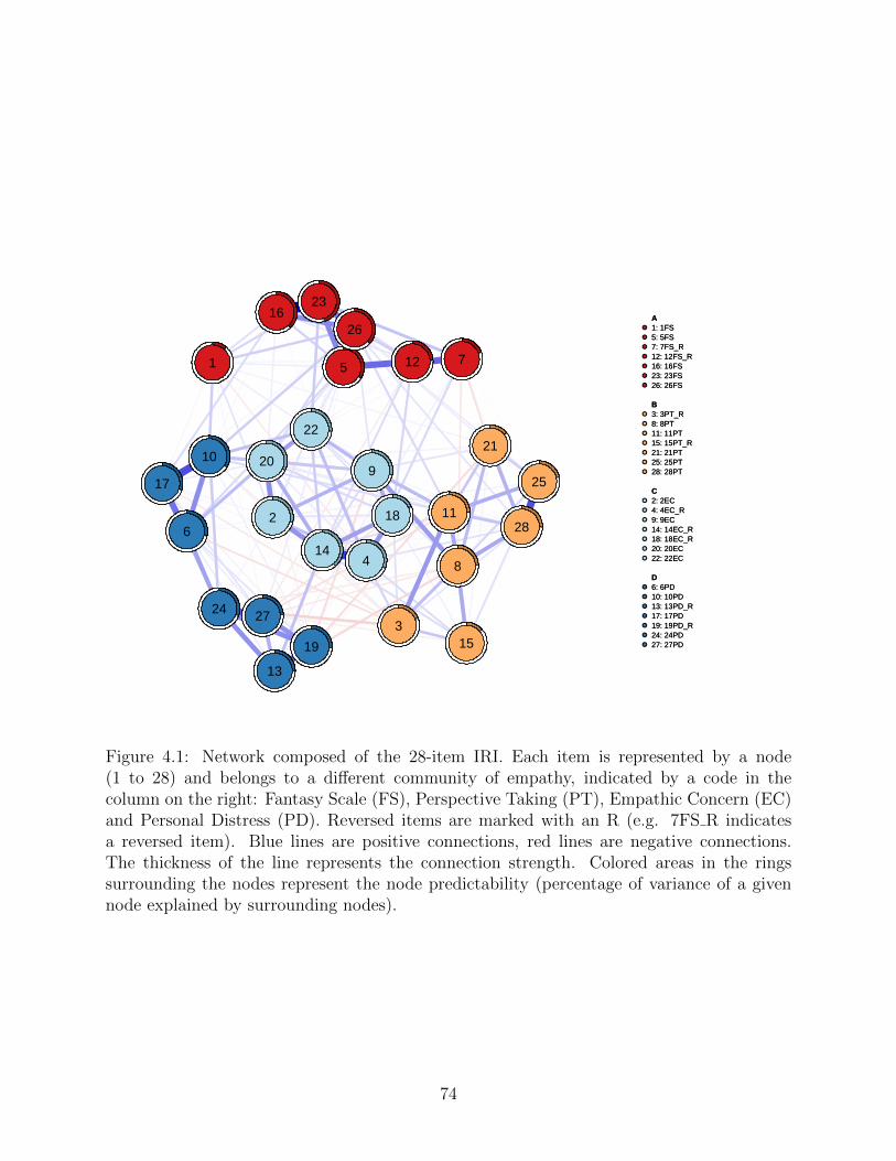
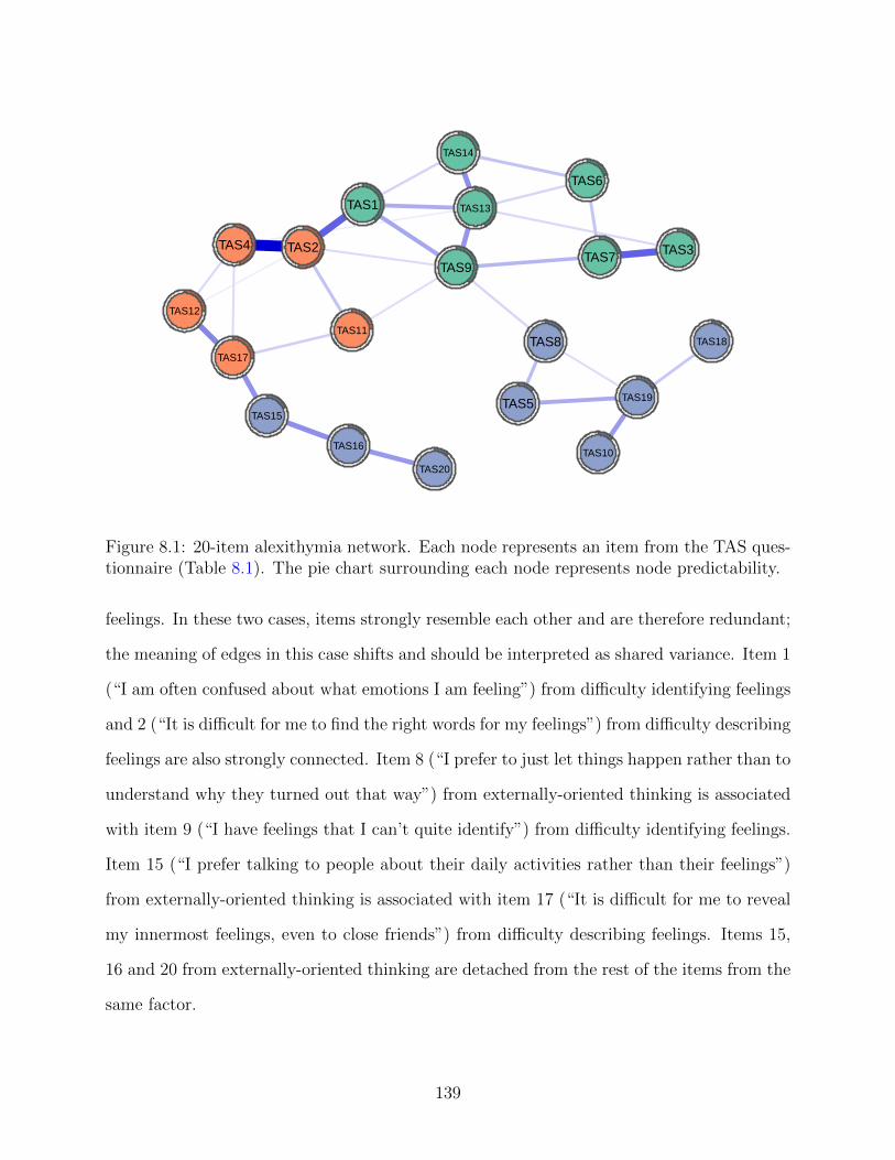
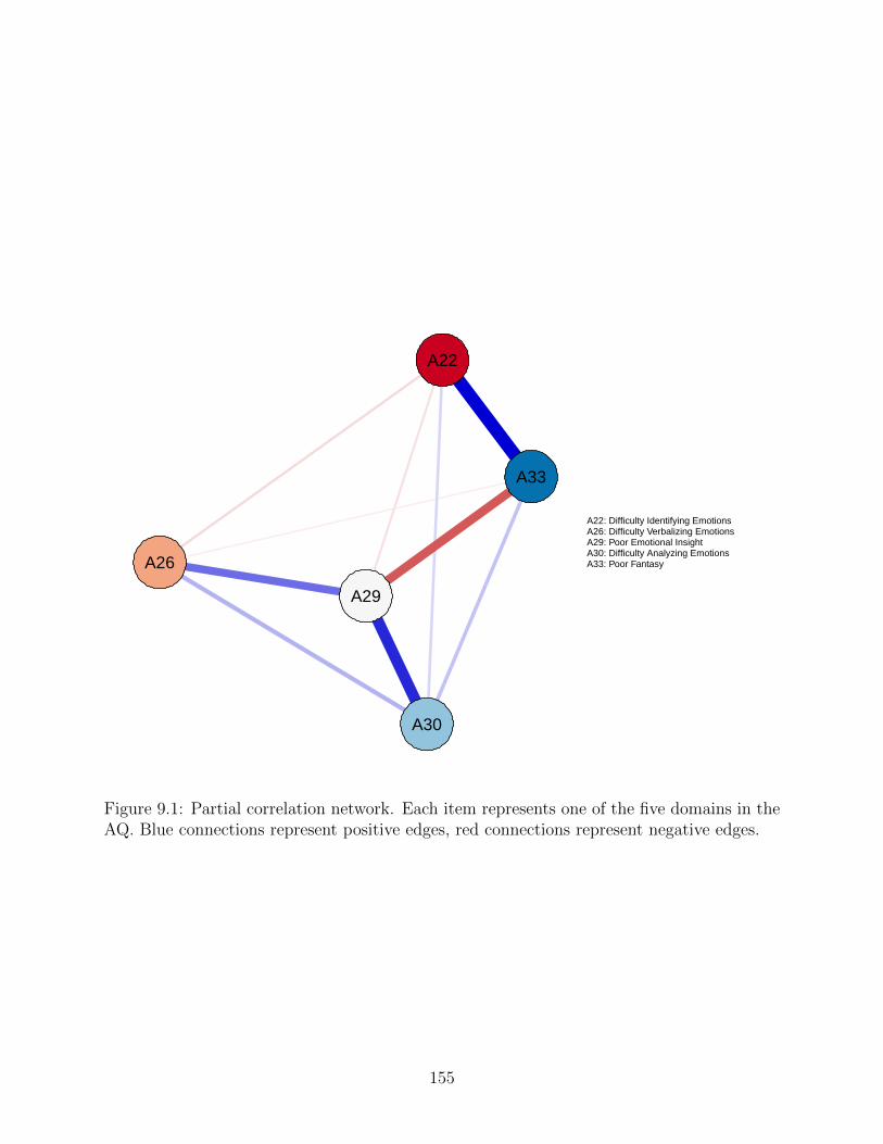
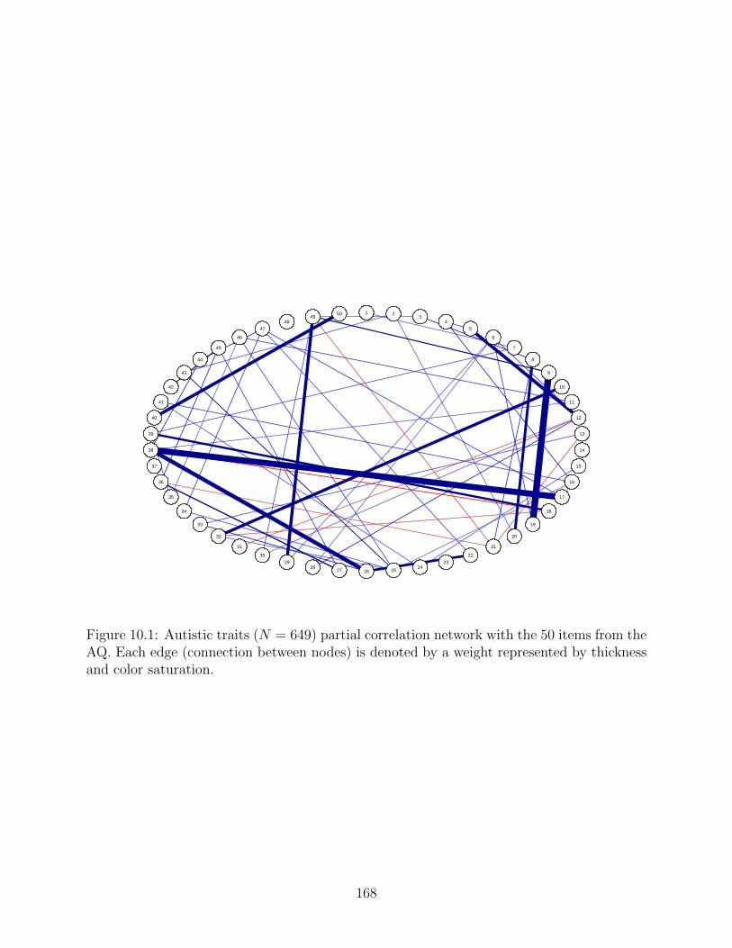
Figure 4.1: Network composed of the 28-item IRI. Each item is represented by a node(1 to 28) and belongs to a different community of empathy, indicated by a code in thecolumn on the right: Fantasy Scale (FS), Perspective Taking (PT), Empathic Concern (EC)and Personal Distress (PD). Reversed items are marked with an R (e.g. 7FS R indicatesa reversed item). Blue lines are positive connections, red lines are negative connections.The thickness of the line represents the connection strength. Colored areas in the ringssurrounding the nodes represent the node predictability (percentage of variance of a givennode explained by surrounding nodes).

74

et al., 2015). Cluster A is composed of items 1, 16, 23, 26, 5, 12, 7, forming the Fantasy

component (FS). Cluster B is formed by items 25, 28, 21, 8, 11, 15, 3, all of which constitute

the Perspective-taking component (PT). Cluster C is formed by items 22, 20, 2, 14, 18, 4, 9

and reflects the Empathic concern component (EC). Cluster D is formed by items 10, 17, 6,

24, 27, 13, 19 and represents the Personal distress component (PD).

The walktrap algorithm identifies 5 communities of items. Most items belong to the same

communities in the spinglass solution above, whereas items 6 (“In emergency situations, I

feel apprehensive and ill-at-ease”), 10 (“I sometimes feel helpless when I am in the middle

of a very emotional situation”) and 17 (“Being in a tense emotional situation scares me”)

form a new community of items (community 5).

Furthermore, in some cases, two items from different communities (as identified by the

spinglass algorithm) have a positive connection: for example, this is the case of item 1 (“I

daydream and fantasize, with some regularity, about things that might happen to me”) and

item 10 (“I sometimes feel helpless when I am in the middle of a very emotional situation”),

item 23 (“When I watch a good movie, I can very easily put myself in the place of a leading

character”) and item 22 (“I would describe myself as a pretty soft-hearted person”), item 8

(“I try to look at everybody’s side of a disagreement before I make a decision”) and item 9

(“When I see someone being taken advantage of, I feel kind of protective towards them”).

Mean node predictability is 0.27, which means that on average, 27% of the variance of each

node is explained by its neighbors: assuming that all edges go to the node under investigation

from its neighbors, I can see how well the given node can be predicted by the other nodes

surrounding it (Haslbeck and Fried, 2017).

4.3.2 Network inference

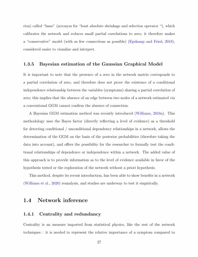
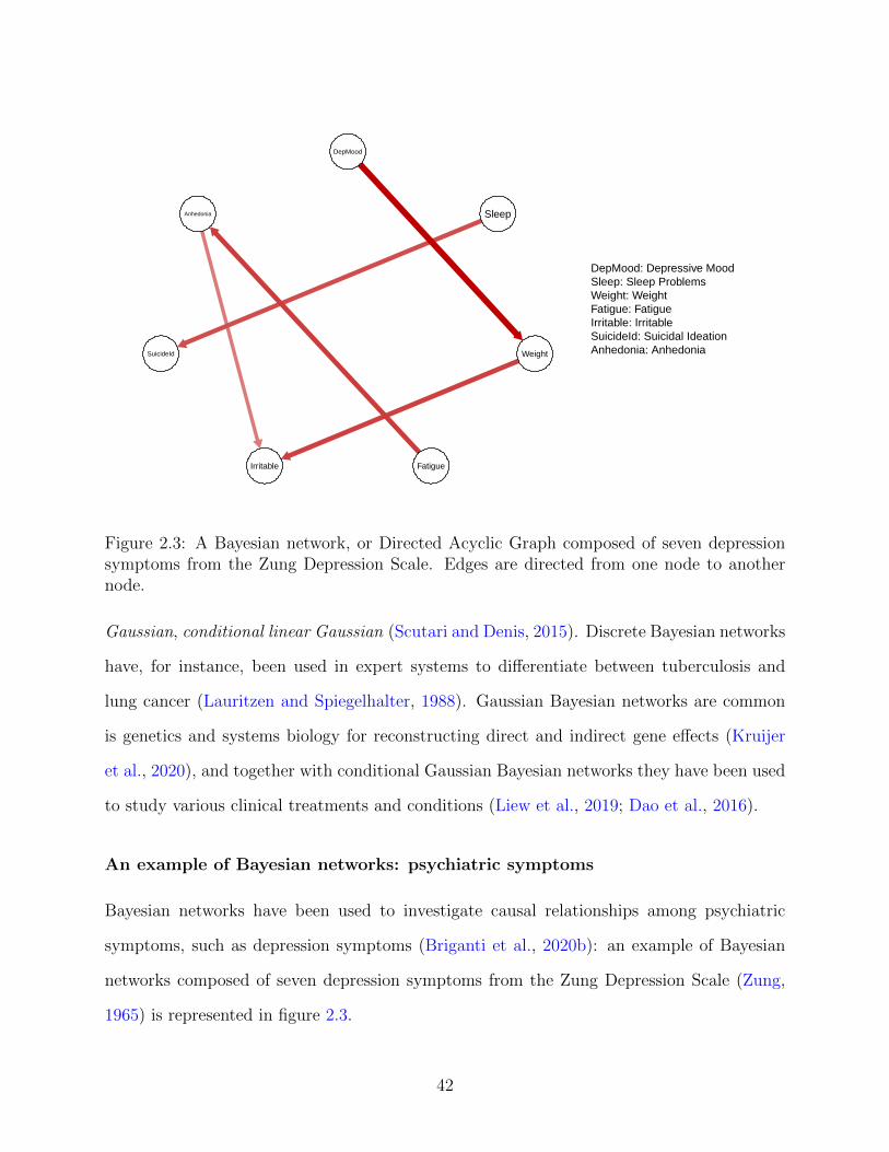
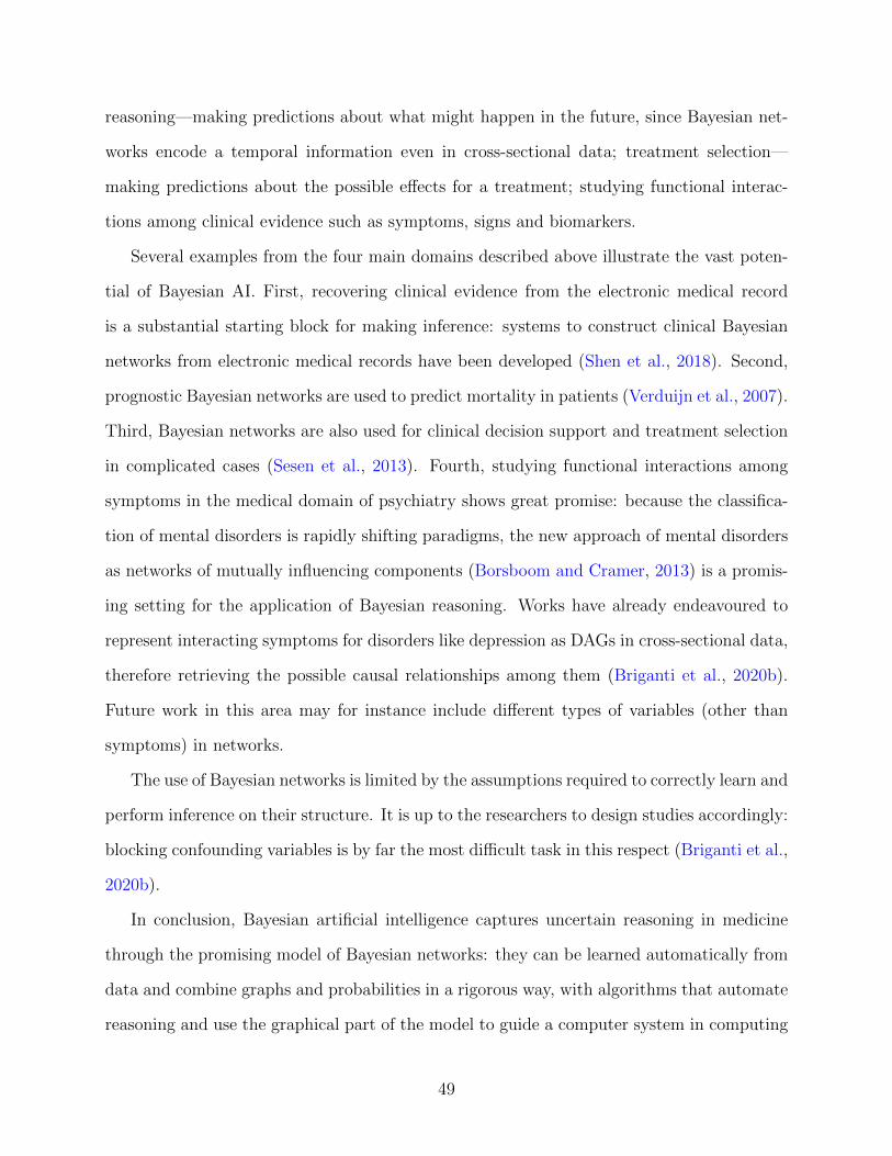
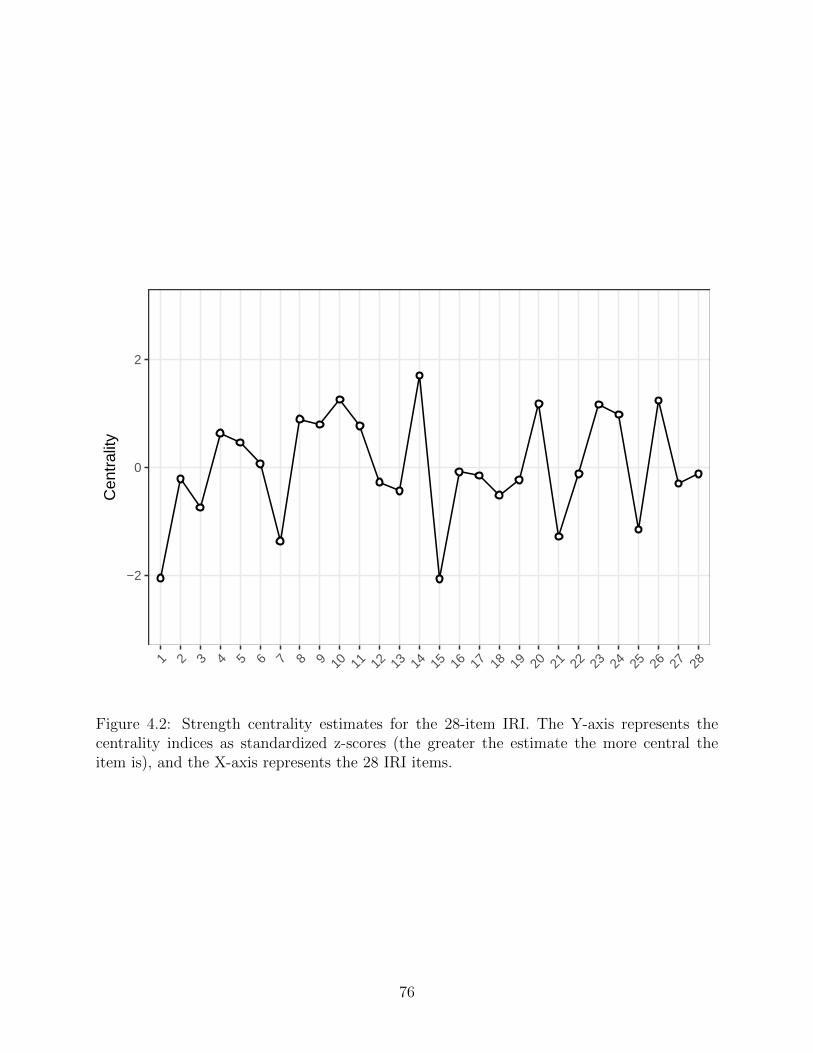
In Figure 4.2, I illustrate the strength centrality estimates for the 28 questionnaire items.

Item 14 (“Other people’s misfortunes do not usually disturb me a great deal”) has the

highest standardized strength centrality in the network. Other central items include node

75

−2

0

2

1 2 3 4 5 6 7 8 9 10 11 12 13 14 15 16 17 18 19 20 21 22 23 24 25 26 27 28

Cen

tral

ity

Figure 4.2: Strength centrality estimates for the 28-item IRI. The Y-axis represents thecentrality indices as standardized z-scores (the greater the estimate the more central theitem is), and the X-axis represents the 28 IRI items.

76

10 (“I sometimes feel helpless when I am in the middle of a very emotional situation “), and

node 26 (“When I am reading an interesting story or novel, I imagine how I would feel if the

events in the story were happening to me”). Items 1 (“I daydream and fantasize, with some

regularity, about things that might happen to me”) and 15 (“If I’m sure I’m right about

something, I don’t waste much time listening to other people’s arguments”) show the lowest

strength centrality values.

4.3.3 Network accuracy and stability

The edge weight bootstrap revealed relatively small CIs, which indicates a more precise

estimation. The edge weight difference test reveals that the empathy network is accurately

estimated and that the strongest edges are significantly stronger than other edges. The

subset bootstrap shows that the order of item strength centrality is more stable than the

other kinds of centrality values, which is consistent with numerous prior papers (Armour

et al., 2017; Epskamp and Fried, 2018). CS-values obtained are 0.44 for node betweenness,

0.67 for node closeness and 0.75 for node strength. CS-values should preferably be above 0.5

and should not in any case be lower than 0.25: my results are above 0.5 and are therefore very

stable. The centrality difference test shows that highest centrality estimates are statistically

different from lowest centrality estimates, even though a statistical difference is not shown

among nodes with the highest strength centrality estimates.

4.4 Discussion

The network analysis I presented is, to my knowledge, the first one applied to empathy

research. This study highlights connections between empathy components and provides new

insights on how they might interact: some items are more interconnected than others, items

differ in centrality, and interactions exist between items from different empathy components.

Positive connections are found throughout the network, confirming that, in my sample,

77

most items from the IRI share some variance and are connected. However, some items present

weak with others; this means that some nodes are conditionally independent of all other items

in the network. The spinglass algorithm identifies on average four communities of items in the

network, corresponding to the four a priori components of Davis’ construct: Fantasy (cluster

A), perspective taking (cluster B), empathic concern (cluster C) and personal distress (cluster

D). The identification of these four node communities supports, using a different method, the

results of Braun et al.’s confirmatory factor analysis study (Braun et al., 2015). This is not

necessarily surprising, given that network and factor models are, under certain conditions,

mathematically interchangeable (Kruis and Maris, 2016).

Even though communities might be mathematically close to factors, from a network

perspective they mean something entirely different: they are clusters of interrelated items

that stem from mutual dynamics; they actively contribute to the construct of empathy itself.

However, the walktrap algorithm identified five communities, describing a fifth community

formed by items 6, 10 and 17. This is a consequence of the strong connection and clustering

of these three items, which nonetheless share two important connections with the rest of the

Personal Distress cluster (6-24 and 10-24). Some items belonging to a given community are

connected to those from different communities, suggesting — from a network perspective —

that empathy communities interact with each other in the network through specific items.

For example, there is a connection between items 8 and 9, respectively belonging to the

Perspective taking and Empathic concern subscales.

Items belonging to the Empathic concern community (9, 14 and 20) have high centrality

values; this finding supports Cliffordson’s theory that puts Empathic concern at the basis (in

this case, at the center) of empathy. Items from the Empathic concern cluster are connected

to all the other communities in the network. Item 14 shows the highest centrality value: to

interpret this finding, one must associate the statistical meanings of centrality and network

connections (edges). First, strength centrality (the main subtype used) means that the sum

of all edges of item 14 to all other nodes is the highest in the IRI network; second, a connection

78

between item 14 and another item means for instance that a high-score answer to item 14

(which is reversed) lets us guess a high-score answer to all the items item 14 is connected

to, controlling all other nodes. I can then interpret the high centrality of item 14 as the one

that might influence and/or might be influenced by most answers of the IRI. However, when

I look at the centrality difference test, I understand that the strength centrality of node 14

is not statistically different than strength centralities of nodes 10, 26, 20, 23 and 24, but is

statistically different from that of all other nodes: this means that these nodes are roughly

equivalent in their centrality. Node predictability, especially when focusing on the average,

is somewhat more straightforward to interpret: on average, if I influence a group of nodes

surrounding a given node, and assume that all edges go towards this node, I can influence

27% of its variance (Haslbeck and Waldorp, 2016).

Stability analysis shows that both centrality and edge weight estimates were reasonably

stable. My results must be interpreted in the light of a number of limitations. First, my

empathy network is estimated from a sample of young adults, which likely limits the general-

izability of my results; further studies should investigate networks structures across different

samples. Second, because I used cross-sectional data to carry out the analyses, I cannot

determine the direction of edges. For instance, I cannot interpret whether the most central

item activates other items, is activated by other items, or both. Third, similar to many other

statistical models such as factor models, the network model used here estimates between-

subjects effects on a group level. This means that network properties such as structure or

centrality may not replicate in the same way in single individuals. Fourth, Marshall et al.

provided evidence that the order in which items are presented in a questionnaire may influ-

ence their relationships (Marshall et al., 2013). Again, this is a limitation for any statistical

model based on the correlation matrix among items, such as factor models, and not a spe-

cific shortcoming over network models, but important enough to warrant mentioning. Fifth,

network analysis, in which I interpret edges as putative causal connections, is based on the

premise that nodes differ from each other meaningfully: if two nodes represent the same

79

aspect of a construct, an edge is not a putative causal connection, but simply represents

shared variance (Fried and Cramer, 2017). IRI might in some cases have this problem, for

instance item 7 (“I am usually objective when I watch a movie or play, and I don’t often get

completely caught up in it”) and item 12 (“Becoming extremely involved in a good book or

movie is somewhat rare for me”) seem to measure the same concept.

Future research may also endeavor to apply empathy networks in people with psy-

chopathology.

80

Chapter 5

A network model of self-worth

Abstract

This study investigates the Contingencies of Self-Worth Scale (CSWS) in a sample

of 680 university students from a network perspective. I estimated regularized partial

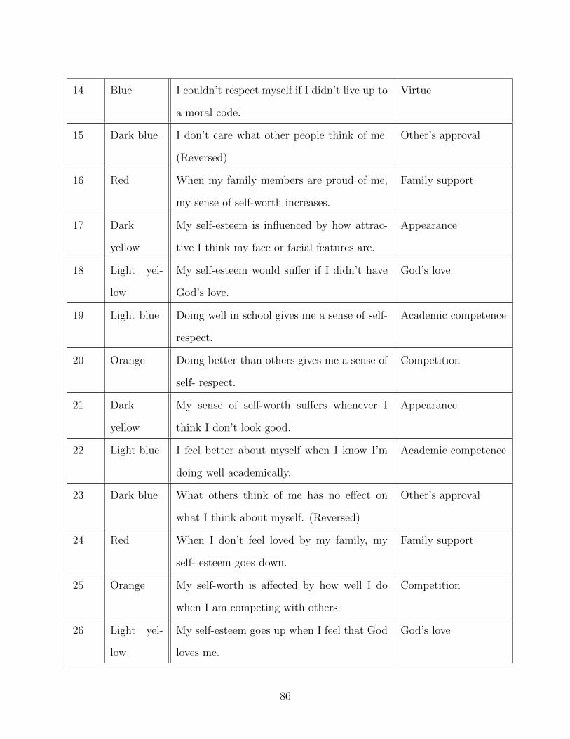
correlations among seven CSWS domains: family support, competition, appearance,

God’s love, academic competence, virtue and other’s approval. Competition - academic

competence and competition – appearance represent the strongest connections in the

network. Mean node predictability (shared variance with surrounding nodes) is 0.25.

Appearance and academic competence were the most central (i.e. interconnected)

domains in the network. Future studies should explore the network structure of self-

worth in other healthy adult samples, and also in people with psychopathology.

5.1 Introduction

The human desire to feel worthy is an important constituent of human behavior (Pyszczynski

et al., 2004). A troubled self-esteem has been shown to contribute to several psychiatric

disorders such as eating disorders (Pearl et al., 2014), substance abuse (James, 2011), and

schizophrenia (Xu et al., 2013).

The Contingencies of Self-Worth Scale (CSWS) is a psychometric tool proposed by

81

Crocker and colleagues (Crocker et al., 2003) to assess seven domains of self-esteem: (1)

family support measures the influence of perceived approval, support and love from family

members on the feeling of self-worth (e.g. item 7 “Knowing that my family members love

me makes me feel good about myself”); (2) competition evaluates how self-worth is influ-

enced by feeling better than others (e.g. item 12 “Knowing that I am better than others on

a task raises my self-esteem”); (3) appearance quantifies how physical traits influence the

way people evaluate themselves (e.g. item 1 “When I think I look attractive, I feel good

about myself”); (4) God’s love measures the association between religiosity and self-esteem

(e.g. item 2 “My self-worth is based on God’s love”); (5) academic competence evaluates

the impact of grades on self-esteem (e.g. item 20 “Doing well in school gives me a sense

of self-respect”); (6) virtue measures the connection between self-worth and the adherence

to a moral code (e.g. item 5 “Doing something I know is wrong makes me lose my self-

respect”); (7) other’s approval measures the influence of perceived approval from others on

self-esteem (e.g. item 9 “I can’t respect myself if others don’t respect me”). This model of

self-esteem has already undergone structural validation (Crocker et al., 2003) which makes

it an interesting tool for exploring the construct of self-esteem (Geng and Jiang, 2013).

A common understanding of self-esteem is that the seven domains are all observable in-

dicators of self-esteem, that is, the domains of the questionnaire do not actively contribute

to the construct — they are effects of the construct. In the last decade, a new way of

conceptualizing psychological constructs has been proposed: network theory, which hypoth-

esizes psychological constructs as interacting systems. Network models are related statistical

models that can be used to try to uncover such structures in data: a network is formed by

pairwise interactions of its components (Borsboom and Cramer, 2013) usually calculated as

regularized partial correlations (Epskamp and Fried, 2018). Components of a network mu-

tually influence each other to actively participate in the emergence of a construct. Mental

disorders such as depression (Beard et al., 2016; Boschloo et al., 2016; Fried and Cramer,

2017; Mullarkey et al., 2018), schizophrenia (Galderisi et al., 2018), posttraumatic stress dis-

82

order (Fried et al., 2018), autism, and obsessive-compulsive disorder (Ruzzano et al., 2015)

have been conceptualized and analyzed statistically from a network perspective. Network

structures of psychological constructs such as empathy (Briganti et al., 2018), personality

(Costantini et al., 2015), health-related quality of life (Kossakowski et al., 2016), intelligence

(van der Maas et al., 2006), and attitudes (Dalege et al., 2017) have also been studied.

Researchers usually analyze constructs as network composed of items — answers of the

observed group to a given questionnaire such as the Interpersonal Reactivity Index (Briganti

et al., 2018). However, scales in psychology are usually constructed to assess one underlying

dimension; this means that they often feature several highly similar items that might measure

the same thing, which has been discussed as a challenge for network models (Fonseca-Pedrero

et al., 2018). In that case, the meaning of the connection between items changes: an associa-

tion between X and Y simply reflects the shared variance of the two items, and not a genuine

mutual relation (Fried and Cramer, 2017). This limitation also holds for the Contingencies

of Self-Worth Scale where a common cause is plausible: items in a given domain might mea-

sure the same construct, and can therefore also be explored with factor models. My work

thus aims to apply network modeling to the construct of contingent self-worth as described

originally (Crocker et al., 2003) while addressing the challenge of items measuring the same

variable, using both structural equation models and network models. The primary goal is to

explore connections between domains of the CSWS; it is plausible to conceptualize the con-

struct of self-worth as a network and consider that its various domains interact and influence

each other instead of being separate consequences with the same origin. Second, I want to

estimate the expected influence (EI) of domains in the network, which can be thought of as

the importance of a domain in the network. EI is calculated as the sum of all connections

of a domain (Robinaugh et al., 2016). Finally, I want to estimate domain predictability

(Haslbeck and Fried, 2017), which reflects the percentage of shared variance of a domain

with surrounding domains in the network. Although I expected EI and predictability to be

related (i.e. domains high on either are likely high on the other), EI provides a measure of

83

the relative importance of a construct, whereas predictability provides insights into absolute

value (Haslbeck and Fried, 2017).

5.2 Method

5.2.1 Participants

This study is based on a data set composed of 680 French-speaking university students: 59%

of them were women and 41% men. The subjects were 17 to 25 years old (M = 19 years, SD

= 1.5 years).

5.2.2 Measurement

The CSWS is composed of 35 items meant to assess self-worth contingency in the following

seven domains: family support, competition, appearance, God’s love, academic competence,

virtue and other’s approval. The items are shuffled in the questionnaire. Item score ranges

from 1 (strongly disagree) to 7 (strongly agree); some reverse-scored items are included

(items 4, 6, 10, 13, 15, 23 and 30).

The data set was anonymized, and its analysis was approved by the Ethical Committee

of the Erasme university hospital.

Table 5.1: The Contingencies of Self-Worth Scale by

Crocker et al. (Crocker et al., 2003).

Item Domain

color

Item meaning Domain

1 Dark

yellow

When I think I look attractive, I feel good

about myself.

Appearance

84

2 Light yel-

low

My self-worth is based on God’s love. God’s love

3 Orange I feel worthwhile when I perform better than

others on a task or skill.

Competition

4 Dark

yellow

My self-esteem is unrelated to how I feel

about the way my body looks. (Reversed)

Appearance

5 Blue Doing something I know is wrong makes me

lose my self-respect.

Virtue

6 Dark blue I don’t care if other people have a negative

opinion about me. (Reversed)

Other’s approval

7 Red Knowing that my family members love me

makes me feel good about myself.

Family support

8 Light yel-

low

I feel worthwhile when I have God’s love. God’s love

9 Dark blue I can’t respect myself if others don’t respect

me.

Other’s approval

10 Red My self-worth is not influenced by the quality

of my relationships with my family members.

(Reversed)

Family support

11 Blue Whenever I follow my moral principles, my

sense of self-respect gets a boost.

Virtue

12 Orange Knowing that I am better than others on a

task raises my self-esteem.

Competition

13 Light blue My opinion about myself isn’t tied to how

well I do in school. (Reversed)

Academic competence

85

14 Blue I couldn’t respect myself if I didn’t live up to

a moral code.

Virtue

15 Dark blue I don’t care what other people think of me.

(Reversed)

Other’s approval

16 Red When my family members are proud of me,

my sense of self-worth increases.

Family support

17 Dark

yellow

My self-esteem is influenced by how attrac-

tive I think my face or facial features are.

Appearance

18 Light yel-

low

My self-esteem would suffer if I didn’t have

God’s love.

God’s love

19 Light blue Doing well in school gives me a sense of self-

respect.

Academic competence

20 Orange Doing better than others gives me a sense of

self- respect.

Competition

21 Dark

yellow

My sense of self-worth suffers whenever I

think I don’t look good.

Appearance

22 Light blue I feel better about myself when I know I’m

doing well academically.

Academic competence

23 Dark blue What others think of me has no effect on

what I think about myself. (Reversed)

Other’s approval

24 Red When I don’t feel loved by my family, my

self- esteem goes down.

Family support

25 Orange My self-worth is affected by how well I do

when I am competing with others.

Competition

26 Light yel-

low

My self-esteem goes up when I feel that God

loves me.

God’s love

86

27 Light blue My self-esteem is influenced by my academic

performance.

Academic competence

28 Blue My self-esteem would suffer if I did some-

thing unethical.

Virtue

29 Red It is important to my self-respect that I have

a family that cares about me.

Family support

30 Dark

yellow

My self-esteem does not depend on whether

or not I feel attractive. (Reversed)

Appearance

31 Light yel-

low

When I think that I’m disobeying God, I feel

bad about myself.

God’s love

32 Orange My self-worth is influenced by how well I do

on competitive tasks.

Competition

33 Light blue I feel bad about myself whenever my aca-

demic performance is lacking.

Academic competence

34 Blue My self-esteem depends on whether or not I

follow my moral/ethical principles.

Virtue

35 Dark blue My self-esteem depends on the opinions oth-

ers hold of me.

Other’s approval


Data were analyzed with R software (open source, available at https://www.r-project.

org/). Packages used to carry out the analysis include qgraph (Epskamp et al., 2012), and

glasso (Friedman et al., 2014b) for network estimation and visualization, mgm for node

predictability (Haslbeck and Waldorp, 2016), igraph (Csardi and Nepusz, 2006) and bootnet

(Epskamp and Fried, 2018) for stability.

87



Sum score vs factor analysis

Items from CSWS subdomains tend to measure the same construct, which is a situation

which a network of all individual items can be problematic because different nodes measure

the same underlying psychological construct (Fried and Cramer, 2017). Therefore, I chose

to estimate a network of 7 domains instead of a network of 35 items. The preferred way for

doing so is using generalized network psychometrics framework (Epskamp et al., 2017b) via

the R-package lvnet. Unfortunately, the method does not currently scale well, and was not

applicable to the current datasets due to the large number of items.

Instead, I studied the network structure of self-worth domains with nodes reflecting sum

scores of the 7 CSWS domains, and used these factor scores as variables in the Gaussian

Graphical Model (GGM), a regularized partial correlation network (Epskamp and Fried,

2018). As an additional sensitivity analysis, I also estimated a factor model using confir-

matory factor analysis for each of the 7 CSWS domains, and then used these factor scores

in a GGM. I expected somewhat stronger relations, because factor scores are disattenuated

for measurement unreliability and therefore likely increase the relations among variables

(Spearman, 1904).

Network estimation

A network structure is composed of nodes and edges: nodes represent, in this case, domains

from the CSWS, and edges are connections between two domains. A regularized partial

correlation network was estimated on the correlation matrix of the 7 domains; as described

above, sumscores for each participant were used. Edge weight parameters that resulted from

the GGM were regularized by using the graphical lasso (least absolute shrinkage and selec-

tion operator): this procedure avoids the estimation of spurious edges (Tibshirani, 2011).

The estimation procedure selected the network (out of 100 networks) with the lowest lambda

value (lambda being the tuning parameter for this procedure); in these situations, it is rec-

ommended to lower the tuning parameter to 0.001, and I followed this recommendation. For

88

the GGM, an edge represents the regularized partial correlation (or conditional dependence

relation) between two domains, controlling for all other domains. If two nodes are connected,

this means they are conditionally dependent, given all other nodes in the network. When

visualizing the model output as graph, blue edges indicate positive relations, and red edges

negative relations. The corresponding thickness of an edge represents its weight (i.e. the

strength of association between nodes, ranging from -1 to 1). The Fruchterman-Reingold

algorithm was used to place nodes in a network (Fruchterman and Reingold, 1991).

Network stability

Stability tests are necessary to safely interpret network inference results from a network

analysis. To answer the question “is edge X significantly stronger than edge Y?”, 95%

confidence intervals of the edge weights were estimated through bootstrapping (Epskamp and

Fried, 2018), 2000 bootstraps were used, and the edge weight difference test was performed.

To answer the question “is the EI of node X stronger than the EI of node Y”, I performed

the centrality difference test.

Network inference

To investigate the network structure of self-worth, I computed two different local inference

measures: node predictability and EI. Expected influence is the sum of a node’s connections

and represents the relative importance of a node in a network (Robinaugh et al., 2016) –

relative because even in weakly connected networks (with overall low edge weights), there

will always be a node with a high expected influence in case of standardized results. Node

predictability is an absolute measure of the interconnectedness of a given node in the net-

work and represents its shared variance with surrounding nodes (Fried et al., 2018). Node

predictability can be interpreted as the upper bound of controllability: if one assumes that

all edges for node X are directed towards that node, predictability provides an estimate of

how much influence I can have on X via all other nodes.

89

5.3 Results

5.3.1 Descriptive statistics

Means range from 12.4 (God’s love) to 26.6 (academic competence). Standard deviations

range from 5.2 (appearance) to 9 (God’s love). God’s love has the lowest mean as well as

the highest standard deviation in the network.

Network of self-worth

Figure 5.1 illustrates the estimated the seven-domain network of self-worth. The network

is composed of domains that connect with each other. Each domain is represented with a

different color. Competition and academic competence share the strongest connection in

the network; other’s approval also shares a strong edge with appearance. Competition and

appearance as well as academic competence and family support are also positively connected.

Family support is positively connected with most domains. God’s love is only connected

to virtue. Appearance and virtue share a negative connection. The factor score network

resulted in considerably stronger associations, which can be expected due to disattenuation.

The adjacency matrices were correlated 0.95 between both methods (sum score and factor

score).

5.3.2 Network stability

Edge weight bootstrap reports relatively small CIs, as is expected from a network with

several hundred participants and only 7 nodes; this means that edge weight estimation is

precise. The edge weight difference test reveals that stronger edges in the network are

significantly stronger than the other edges. In other words, stronger edges in Figure 1 can

be interpreted as being considerably stronger than weaker edges. For instance, the edges

between competition and academic competence and competition and appearance represent

the statistically strongest edge coefficients in the network, significantly stronger than all

90

FS

C

A

GL

AC

V

OA

FS: Family SupportC: CompetitionA: AppearanceGL: God's LoveAC: Academic competitionV: VirtueOA: Other's Approval

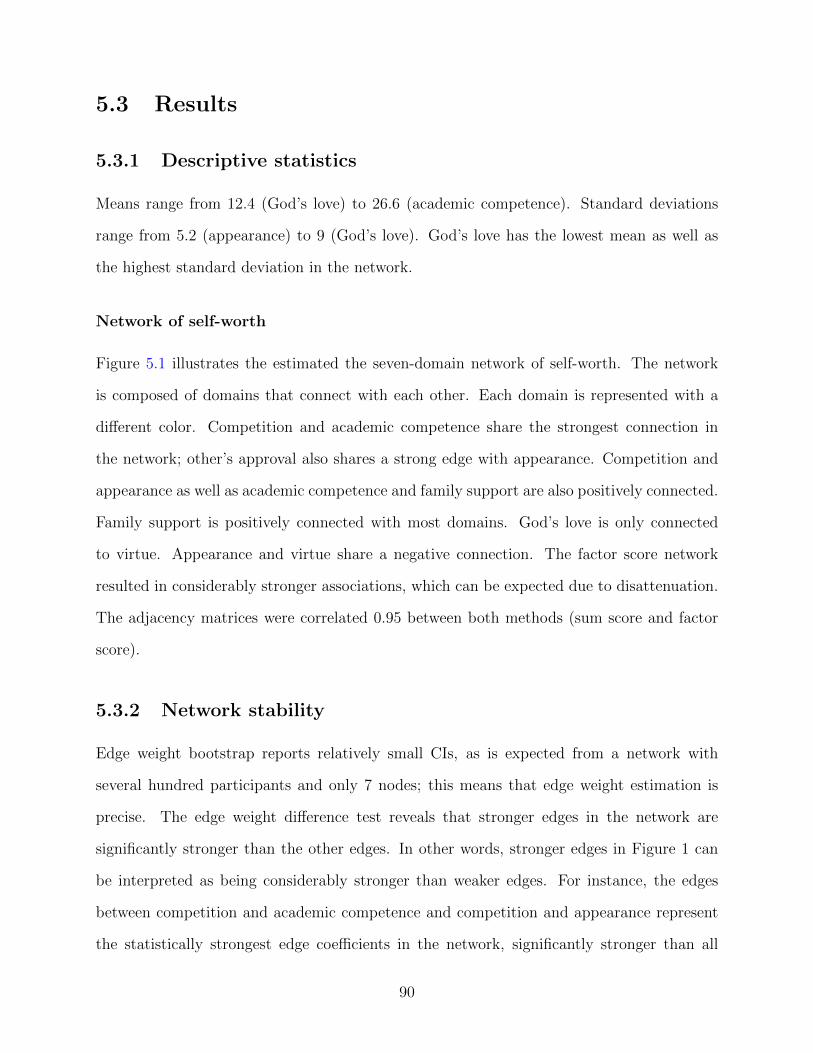
Figure 5.1: 7-domain CSWS network. Each node represents a domain: FS is “Familysupport”, C is “Competition”, A is “Appearance”, GL is “God’s love”, AC is “Academiccompetence”, V is “Virtue” and OA is “Other’s approval” cluster. Blue edges representpositive connections and red edges represent negative connections; the thicker the connec-tion the stronger it is. The pie chart surrounding the node represents node predictability(percentage of shared variance with all connected nodes).

91

−2

0

2

A AC C FS GL OA V

CSWS_Domain

Exp

ecte

d In

fluen

ce

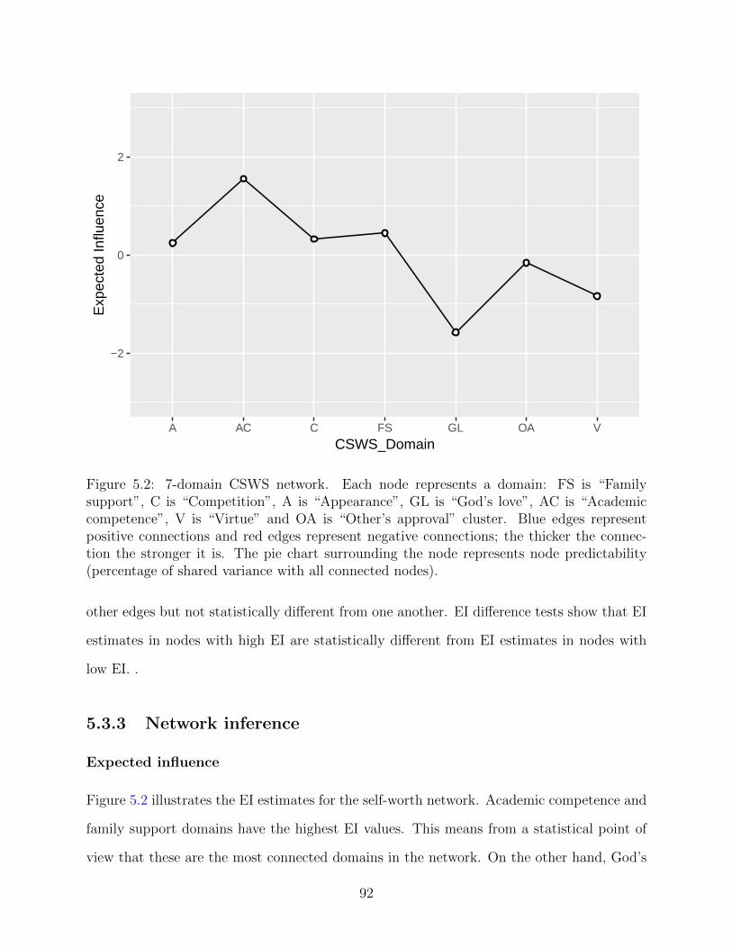
Figure 5.2: 7-domain CSWS network. Each node represents a domain: FS is “Familysupport”, C is “Competition”, A is “Appearance”, GL is “God’s love”, AC is “Academiccompetence”, V is “Virtue” and OA is “Other’s approval” cluster. Blue edges representpositive connections and red edges represent negative connections; the thicker the connec-tion the stronger it is. The pie chart surrounding the node represents node predictability(percentage of shared variance with all connected nodes).

other edges but not statistically different from one another. EI difference tests show that EI

estimates in nodes with high EI are statistically different from EI estimates in nodes with

low EI. .


Expected influence

Figure 5.2 illustrates the EI estimates for the self-worth network. Academic competence and

family support domains have the highest EI values. This means from a statistical point of

view that these are the most connected domains in the network. On the other hand, God’s

92

love has the lowest EI value. This means that it is the domain that least influences the rest

of domains in the network. Correlation between EI and predictability is 0.96.

Node predictability

Mean node predictability ranges from 0.06 to 0.40, with an average of 0.25. This means that

on average, 25% of the variance of the node in the network can be explained by its neighbors.

God’s love is the domain with the lowest node predictability: it shares 6% of variance with

its surrounding nodes. Academic competence has the highest node predictability: it shares

40% of its variance with its surrounding nodes. Competition has the second highest node

predictability (0.35).

5.4 Discussion

To my knowledge, I have conducted the first network analysis of the psychological construct

self-worth contingencies. Overall, the seven domains of self-worth form a heterogeneous

system in which domains are not uniformly positively connected with each other. This is

interesting, because a homogeneous network with uniformly positive connections would be

expected if all domains are passive and interchangeable measures of one latent variable:

self-worth. Below, I discuss the findings in more detail.

Academic competence and competition share the strongest connection in the network:

it is reasonable to consider that the impact on self-esteem of competing with others and

obtaining good grades are connected while following a university curriculum. The same

kind of connection is found between appearance and other’s approval; this means that, while

considering self-worth, if physical appearance is important to an individual, so is the approval

of others, and vice versa. Competition also shares a strong connection with appearance,

which means that physical appearance might be important for individuals competing with

others (and vice-versa). Family support and other’s approval share connections with most

93

domains in the network. Appearance showed a negative connection to virtue: that means

that people that base their self-worth upon acting and living by a moral code might not draw

self-worth from physical appearance (and vice-versa), controlling for all other associations in

the network. While there is no prior work on partial correlations, previous work on zero-order

correlations found a positive association between the two domains (Crocker et al., 2003).

Negative edges have not been observed commonly in the psychopathology network lit-

erature, which calls for an explanation. In this case, the negative association between ap-

pearance and virtue might be plausible from a theoretical perspective. Since both subscales

are positively associated with academic competence and family support, the finding implies

that in individuals whose self-worth is simultaneously contingent on academic competence

and family support, knowing that self-esteem is more contingent on virtue allows predicting

that their self-esteem is less likely to be also contingent on physical appearance (and vice

versa). Two other possibilities also come to mind. First, negative connections in Gaussian

Graphical Models can arise when dealing with small samples and/or when estimating poly-

choric correlations (Epskamp and Fried, 2018), which I can rule out as explanation here.

Second, collider structures in conditional dependence networks can induce spurious negative

relations between two nodes in case they both cause a third node (Greenland et al., 1999).

God’s love is a relatively disconnected node: it shares only one positive connections

with virtue: this is not surprising, since in the original work (Crocker et al., 2003) God’s

love showed its strongest correlation with virtue. From a network perspective, this means

that God’s love is largely conditionally independent from other domains in the network.

From a network perspective, one plausible interpretation of the conditional independence

of God’s Love in the self-esteem network is that people may derive a sense of self-worth

from their religious belief (in this case, feeling that they have the love of God) regardless

of the other contingencies; this may highlight religious belief as an independent source of

self-esteem in people. Another possible interpretation of this finding is statistical, i.e. a floor

effect or a ceiling effect: because of a low or high parameter, the domain might share few

94

connections with other domains. This may be applicable to my findings, since God’s love

has the highest standard deviation among all domains in the network, as well as the lowest

mean. I identified strong differences in predictability, ranging from 6% (God’s love) to 40%

(academic competence). Average node predictability is 0.25, which means that on average,

25% of the variance of the nodes is explained by other nodes in the network. From a network

perspective, I can infer that some domains such as academic competence are well explained

by its surrounding domains. Academic competence and God’s love are respectively the most

and least predictable nodes in the network.

The analysis of EI shows that academic competence, and family support have the highest

values in the network: this means that these two domains share the strongest connections

in the network and therefore may influence or be influenced by other domains of contingent

self-worth the most. Node predictability is therefore simpler to interpret than EI and gives

us a clear information about how a node is influenced by surrounding nodes, assuming all

edges are directed towards this node.

This study should be interpreted in the light of some limitations. First, my network is

estimated from a sample of university students. While the CSWS was originally developed

based on a similar sample (Crocker et al., 2003), it is worth noting that results of my study

may not generalize to other samples. Second, the current cross-sectional data set does not

allow for causal or even Granger-causal inference. For instance, I cannot interpret whether

a given domain causes or is caused by domains sharing a connection with it. This requires

temporal follow-up studies, which would be most interesting across important developmental

periods such as adolescents and early adulthood. Third, the network model I estimated is

a between-subjects models. This also means that inferences from the study should only be

drawn for a group of people, and it is unclear if and how well the present between-subjects

network structure describes individuals’ networks of self-worth contingency.

Future research may endeavor to apply self-worth contingency networks in other kinds

of samples, both healthy and with different kinds of psychopathology, as to analyze possible

95

differences in network structure, node predictability and centrality.

96

Chapter 6

A network model of resilience

Abstract

The Resilience Scale for Adults (RSA) is a questionnaire that measures protective

factors of mental health. The aim of this paper is to perform a network analysis of the

Resilience Scale for Adults (RSA) in a dataset composed of 675 French-speaking Belgian

university students, to identify potential targets for intervention to improve protective

factors in individuals. I estimated a network structure for the 33-item questionnaire

and for the six domains of resilience: perception of self, planned future, social com-

petence, structured style, family cohesion and social competence. Node predictability

(shared variance with surrounding nodes in the network) was used to assess the con-

nectivity of items. An Exploratory Graph Analysis (EGA) was performed to detect

communities in the network: the number of communities detected being different than

the original number of factors proposed in the scale, I estimated a new network with

the resulting structure and verified the validity of the new construct which was pro-

posed. The network composed of items from the RSA is overall positively connected

with strongest connections arising among items from the same domain. The domain

network reports several connections, both positive and negative. The EGA reported

the existence of four communities that I propose as an additional network structure.

Node predictability estimates show that connectedness varies among the items and

domains of the RSA. Network analysis is a useful tool to explore resilience and identify

97

targets for clinical intervention. In this study, the four domains acting as components

of the additional four-domain network structure may be potential targets to improve

an individual’s resilience. Further studies may endeavor to replicate my findings in

different samples.

6.1 Introduction

Resilience is understood as a positive adaptation despite significant adversities or trauma

(Luthar, 2006). Resilience is a psychological construct which has been proven to be related

to psychiatric disorders, such as anxiety, depression, substance abuse obsessive-compulsive

disorder (Hjemdal et al., 2011a; Bonfiglio et al., 2016).

In recent years, the construct of resilience has been conceived as an outcome rather than a

trait, which highlights the ability to improve an individual’s protective factors against mental

illness (Chmitorz et al., 2018). In this framework, protective factors composing resilience

compete with risk factors, for instance, adverse events (such as traumatic experiences, loss

or neglect) which have been shown to be present in up to 50% of individuals under the age

of 18 (Fritz et al., 2018). Other important factors influencing the framework of resilience

involve age, social status and education (Aburn et al., 2016).

The Resilience Scale for Adults (RSA) is a psychometric questionnaire that assesses

protective factors of mental health (Friborg et al., 2003). The RSA has been defined as one of

the best resilience questionnaires with regard to psychometric ratings (Windle et al., 2011).

Largely validated in Norwegian samples, the construct has undergone in the last decade

cross-cultural validation in different countries, such as Belgium (Hjemdal et al., 2011b), Iran

(Jowkar et al., 2010), Italy (Bonfiglio et al., 2016) and Peru (Morote et al., 2017). The

RSA measures six domains of resilience: (1) perception of self represents the confidence in

oneself, one’s own capabilities, judgment and decision-making (e.g. item 17 “My judgment

and decisions I trust completely”); (2) planned future identifies goal-oriented individuals (e.g.

item 32 “My goals for the future are well thought through”); (3) social competence represents

98

the ability to adapt in social environments (e.g. item 21 “Meeting new people is something I

am good at”); (4) structured style identifies with organized individuals who follow routines

(e.g item 23 “When I start on new things/projects, I prefer to have a plan”); (5) family

cohesion measures the loyalty, support, optimism, mutual understanding and appreciation

among family members (e.g. item 3 “My family understanding of what is important in life

is very similar”); (6) social resources identifies the availability of social support from friends

and family (e.g. item 6 “I can discuss personal issues with friends/family members”). These

six domains are commonly understood as being effects of the construct of resilience itself,

since they are measurable indicators of the construct.

However, in recent years, network theory has emerged as a way of studying psychological

constructs as interacting entities (Borsboom, 2017). Such entities are uncovered in real-world

data using network models, usually composed of pairwise interactions of its elements, and

the constructs emerge from these connections (Borsboom and Cramer, 2013). Interactions

between elements composing a network are often statistically represented as regularized

partial correlations (Epskamp and Fried, 2018). Several mental disorders have been analyzed

using a network perspective, such as posttraumatic stress disorder (Fried et al., 2018; Phillips

et al., 2018), depression (Mullarkey et al., 2018), schizophrenia (Galderisi et al., 2018) and

obsessive-compulsive disorder (Ruzzano et al., 2015). Network analysis has also been applied

to several psychological constructs, such as personality (Costantini et al., 2015), empathy

(Briganti et al., 2018), attitudes (Dalege et al., 2017), intelligence (van der Maas et al., 2006)

and self-worth (Briganti et al., 2019). Other studies used innovative methods, including

networks to harmonize rating scales (Gross et al., 2018; Purgato et al., 2018; Haroz et al.,

2016).

Learning the network structure of a given construct (such as resilience) or mental disor-

der (such as PTSD) is particularly relevant in clinical practice since it highlights potential

clinical target that may affect multiple symptoms or elements composing the network (Fried

et al., 2018); for instance, intervening on the connection between two components of the

99

network is likely to modify the clinical presentations of said components (such as symp-

toms). In the specific case of resilience, which is considered a protection against mental

disorders, learning the network structure of resilience components may highlight potential

targets to strengthen the overall mental health of a given individual. In recent years, several

intervention methods to foster resilience have been studied worldwide, but their efficiency is

variable because of limited comprehension of this relevant psychological construct (Chmitorz

et al., 2018). A network analysis of resilience factors has also been proposed in two sample

of adolescent subjects with and without childhood adversities (Fritz et al., 2018) and showed

that childhood adversities impact the degree of connectivity of resilience factors.

Network components are usually answers of an observed group to items of a questionnaire,

such as the RSA. A current challenge in network models when dealing with self-report

scales is the redundancy of several items of a given questionnaire in measuring the same

aspect of a construct (Fonseca-Pedrero et al., 2018); while addressing the meaning of a

given connection between two items, their interaction will represent shared variance (and

not a pairwise relationship) if they tend to measure the same thing (Fried and Cramer,

2017). In the case of the RSA, this challenge goes beyond the notion of a single items of the

questionnaire and may apply to entire domains of the RSA: for instance, questions from both

perception of self and planned future refer to one’s own dispositional attributes and internal

source of resilience and were original part of the same factor, which was called personal

competence (Friborg et al., 2003). The same line of reasoning applies to family cohesion

and social resources, even though originally distinct factors, since they represent an external

source of resilience – that is, the support that the individual feels both within and without

the family nucleus: furthermore, several items from social resources include the concept of

family support (e.g. item 6 “I can discuss personal issues with friends/family). Exploratory

graph analysis (EGA) has emerged as a highly effective and reliable tool in network analysis

when addressing the issue of recovering the number of factors (CFA) in datasets (Golino and

Epskamp, 2017). An optimum solution proposed in the literature is to first explore the basic

100

dimensionality of an instrument with an EGA then authenticate the suggested structure by

performing a confirmatory factor analysis (Golino and Demetriou, 2017).

I aim to extend the conceptual framework of network analysis to the construct of re-

silience such as represented by the RSA and address the challenge of domain redundancy

using both network models and structural equation models. First, I want to explore the con-

nectivity of the RSA as a network composed of its items, then study the connections arising

among resilience domains, such as performed in recent network papers (Briganti et al., 2019).

Second, I want to apply community detection algorithms and the EGA to the item network,

explore then verify the suggested structure with CFA and network analysis. Third, I want

to measure node predictability which an absolute measure of interconnectedness (Haslbeck

and Fried, 2017) of a node in a network.

Statistically speaking, node predictability represents the shared variance of a network

component with surrounding components. Although performed on university students, ex-

ploring a network structure that shows how domains of resilience interact may have mean-

ingful clinical implications as it highlights potential target to improve the overall protective

factors of a given individual; also, it may serve as basis for future replication studies designed

to identify the network structure of RSA in other samples.

6.2 Method

6.2.1 Participants

The analyses in this paper are performed on a dataset composed of 675 university students

from the French-speaking region of Belgium. 59% of the students were women and 41% were

men; subjects were 17 to 25 years old (M=19 years, SD=1.5 years).

101

6.2.2 Measurement

The RSA is composed of 33 items that measure resilience in 6 domains: perception of self,

planned future, social competence, structured style, family cohesion and social competence.

The items are shuffled in the questionnaire. Item scoring is semantic and differential-based

(Friborg et al., 2006a): for instance, when scoring item 13 “My family is characterized by”,

a minimum score of 1 is represented by the answer “Disconnection” and a score of 7 is

represented by the answer “Healthy cohesion”. Reversed-score items are included in the

scale.

This study was approved by the Ethical Committee of the Erasme university hospital.


I used the software R (open source, available at https://www.r-project.org/). Pack-

ages and functions to carry out the analysis include qgraph (Epskamp et al., 2012), glasso

(Friedman et al., 2014b) for network estimation and visualization, mgm (Haslbeck and Wal-

dorp, 2016) for node predictability, EGA (Golino and Epskamp, 2017) and igraph (Csardi

and Nepusz, 2006) for community detection, and bootnet (Epskamp and Fried, 2018) for

stability.

Item network

I calculated correlations for the 33 RSA items and used the resulting correlation matrix as

an input to estimate a Gaussian Graphical Model (GGM), a regularized partial correlation

network (Epskamp and Fried, 2018). Graphical lasso (least absolute shrinkage and selection

operator) was used to regularize the parameters resulting from the GGM, therefore avoiding

the estimation of spurious connections (non-existing connections that may be present due

to noisy information). In the item network, nodes represent resilience items from the RSA

questionnaire. Each node is surrounded by a pie chart representing node predictability.

Connections between nodes are called edges. An edge in a network is interpreted as the

102


existence of an association between two nodes, controlling for all other nodes in the network.

An edge between two items of the RSA may be statistically interpreted as following: if

two given nodes X and Y share an edge XY in the network, and the observed group of

subjects scores high on X, then the observed group is also more likely to score high on Y

(Briganti et al., 2018). Each edge in the network represents either positive regularized partial

correlations (visualized as blue edges) or negative regularized partial correlations (visualized

as red edges). The thickness and color saturation of an edge denotes its weight (the strength

of the association between two nodes). The Fruchterman-Reingold algorithm places the

items in the network based on the sum of connections of a given node with other nodes

(Fruchterman and Reingold, 1991).

Six-domain network

To assess the overall connectedness of the domains of resilience as described in the RSA

(Hjemdal et al., 2011a) I used the methodology described in recent papers (Briganti et al.,

2019) and estimated a factor model using CFA for each of the six RSA domains. I then used

the factor scores obtained to estimate an additional GGM.

Network stability

Network stability is composed of several state-of-the-art analyses which are necessary to

safely interpret results from a network analysis. I estimated 95% confidence intervals (CI)

of the edge weight through bootstrapping (Epskamp and Fried, 2018), 2000 bootstraps were

used and performed an edge weight difference test to answer the question “is edge A signifi-

cantly stronger than edge B?”.

Network inference

I estimated node predictability for the 33 RSA items and for the six domains. Node pre-

dictability (Haslbeck and Fried, 2017) represents shared variance of a given node with sur-

103

rounding nodes in a network. Node predictability is an absolute measure of the interconnect-

edness of network nodes (Fried et al., 2018). Other measures of inference frequently used in

network literature such as strength centrality (Boccaletti et al., 2006) or expected influence

(Robinaugh et al., 2016) can only address the relative importance of nodes (Briganti et al.,

2019) and are therefore less informative when it comes to address the issue of interconnect-

edness; that is why I decided not to use these measures in this paper. One interpretation

of node predictability that has been previously described in the literature (Briganti et al.,

2019) is that of the upper bound of controllability: this measure can provide an estimate

of how much a node X can be influenced by all other nodes if I assume that all edges that

node X shares with other nodes are directed towards X. To explore the dimensionality of

the RSA in my sample I performed an EGA on the item network. EGA uses the walktrap

algorithm to detect communities. This algorithm is based on the principle that adjacent

nodes tend to belong to the same community (Yang et al., 2016), was shown to have high

accuracy in simulation studies (Golino and Epskamp, 2017) and used in empirical network

papers (Briganti et al., 2018).

Four-domain network

Because I detected a different structure – composed of four domains instead of six as the

one originally proposed (Hjemdal et al., 2011a), I used CFA to estimate a four-factor model

and used the resulting factor scores to estimate a four-domain network; because the network

estimation procedure selected the network (out of a 100 networks) with the lowest tuning

parameter (called lambda value), I lowered the lambda value to follow standard recommen-

dations. I also calculated node predictability for the four nodes of the resulting network.

104

F1 F2

F3

F4

F5

F6

F7

F8

F9

F10

F11

F12

F13

F14 F15

F16

F17

F18

F19

F20

F21

F22

F23

F24

F25F26

F27

F28

F29

F30F31

F32 F33

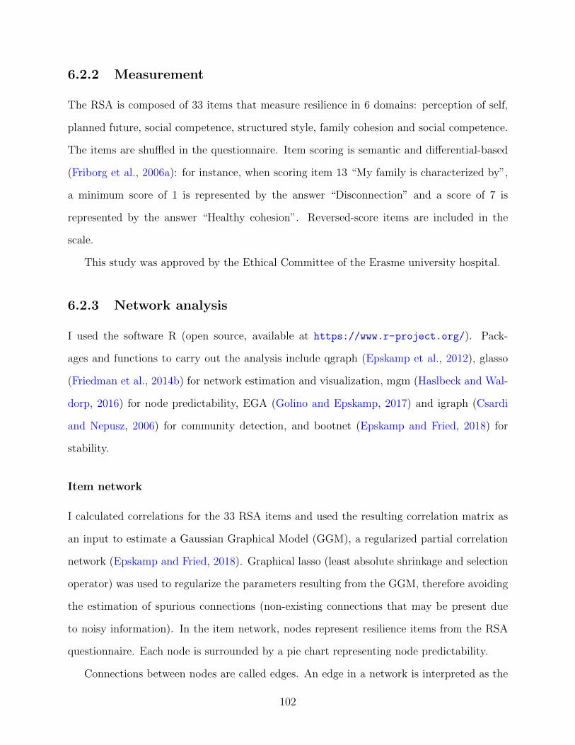
Figure 6.1: 33-item RSA network. Each node represents an item from the questionnaire.Blue edges represent positive connections and red edges represent negative connections; thethicker the connection the stronger it is. The pie chart surrounding the node represents nodepredictability (percentage of shared variance with all connected nodes).

105

6.3 Results

6.3.1 Item network

Figure 6.1 represents the item network: to render the visualization more readable, I hid

all edges smaller than 0.05 (one tenth of the value of the maximum edge weight). Overall,

the 33 items from the RSA form a network of positively connected nodes. The strongest

connection (0.5) is the edge between node 18 (“New friendships are something I make easily”)

and node 21 (“Meeting new people is something I am good at”), both belonging to social

competence. Two other examples of strong connections are edge 9-15 belonging to social

resources (“Those who are good at encouraging me are some close friends/family; “I get

support from friends/family members”) and edge 4-32 belonging to planned future (“I feel

that my future looks very promising”; “My goals for the future are very thought through”).

These examples of highly connected nodes reflect the challenge of items representing the same

aspect of a construct and are discussed in section 4. However, several edges connect different

domains of resilience. For instance, edge 11-19 connects perception of self and social resources

(“My personal problems I know how to solve”; “When needed, I have always someone who

can help me”), and edge 17-26 connects perception of self and social competence (“My

judgment and decisions I trust completely”; “For me, thinking of good topics of conversation

is easy”).

6.3.2 Six-domain network

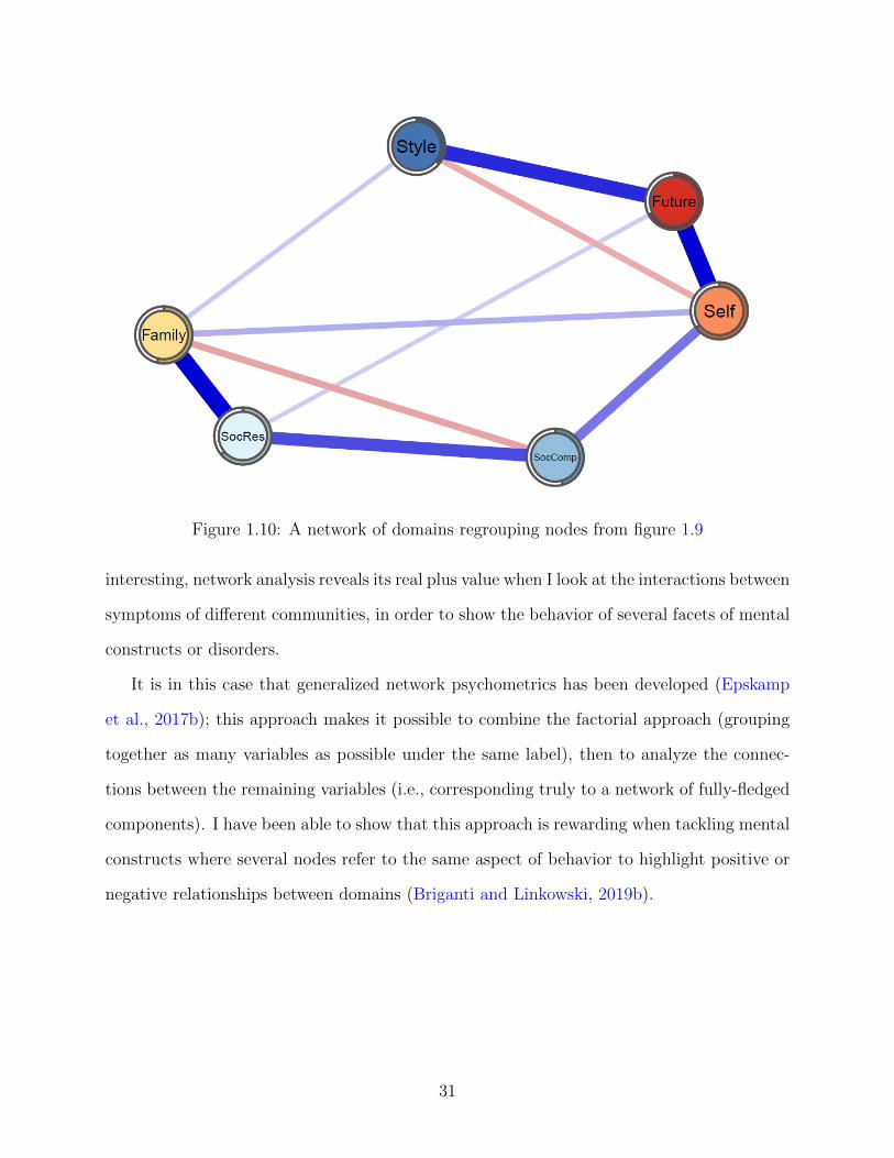
Figure 6.2 illustrates the six-domain network of resilience. This network reports considerably

stronger connections because of disattenuation due to measurement unreliability. This issue

is to be expected when dealing with a GGM based on correlations between factor scores and

has been previously described in the literature (Briganti et al., 2019).

The strongest connections are found between social resources and family cohesion (0.59),

and between planned future and perception of self, (0.58). Two negative connections are

106

Future

SelfFamily

SocRes

SocComp

Style

Future: Planned FutureSelf: Perception of SelfFamily: Family CoherenceSocRes: Social ResourcesSocComp: Social CompetenceStyle: Structured Style

Figure 6.2: Six-domain RSA network. Each node represents a domain from the RSA.

found between structured style and perception of self (0.19) and between family cohesion

and social competence (0.21). Several domains present no direct connection with each other,

such as structured style and social competence or social resources and perception of self;

from a network perspective, that means that the two domains are conditionally independent

from each other.

I performed a CFA to assess the validity of the six-domain structure. Root Mean Square

Error of Approximation (RMSEA) is 0.047 (cut-off for good fit < 0.06) and the Standardized

Root Mean Square Residual (SRMSR) is 0.058 (cut-off for good fit <0.08); Cronbach’s alpha

is 0.64 (>0.8 for good fit); Comparative Fit Index (CFI) is 0.87 (>0.9 for good fit) and the

p-value for the chi-square fit test is 0 (> 0.05 for good fit; Schreiber, 2017).


Bootstrapped 95% edge weight CI show that the edge weights are accurately estimated, and

the edge weight difference tests report that stronger edges can be safely interpreted as to

be stronger that other edges in both the item network and the six-domain network, but do

not statistically differ from each other in the six-domain network. For instance, one cannot

safely interpret the edge between social resources and family cohesion to be stronger than

107

the edge between perception of self and planned future.


Node predictability

Node predictability was estimated in both the item network and the six-domain network.

In the item network, the two nodes with the highest node predictability are node 18 (“New

friendships are something I make easily”; 0.54) and 21 (“Meeting new people is something

I am good at”; 0.53), which both belong to social competence and also share the strongest

edge in the network. The node with the lowest node predictability is node 33 which belongs

to perception of self (“Events in my life that I cannot influence I manage to come to terms

with”; 0.13). Mean node predictability is 0.32, which means that on average, items from

the RSA share 32% of their variance with surrounding nodes. In the six-domain network,

planned future shows the highest node predictability (0.67) and structured style is the least

predictable node (0.36). The mean node predictability is 0.55, which means that on average,

domains present 55% of shared variance.

Community detection

The EGA and walktrap algorithm applied to the item network report four communities of

items instead of six as proposed in the original scale. To visualize the differences between

communities, I first reestimate the network with a different color palette, each color indicating

a community of items as detected by the algorithm as shown in Figure 6.3.

Overall, items from perception of self and planned future form a new community, that

I identify as personal competence, referring to one of the first versions of the RSA (Friborg

et al., 2006b); the same process applies to items from social resources and family cohesion,

forming a new community that I identify as support since it is an aspect of resilience that

the two domains represent. Items 10 (“The bonds among my friends are strong”) and 19

(“When needed, I have always someone who can help me”) switch communities, going from

108

F1 F2

F3

F4

F5

F6

F7

F8

F9

F10

F11

F12

F13

F14 F15

F16

F17

F18

F19

F20

F21

F22

F23

F24

F25F26

F27

F28

F29

F30F31

F32 F33

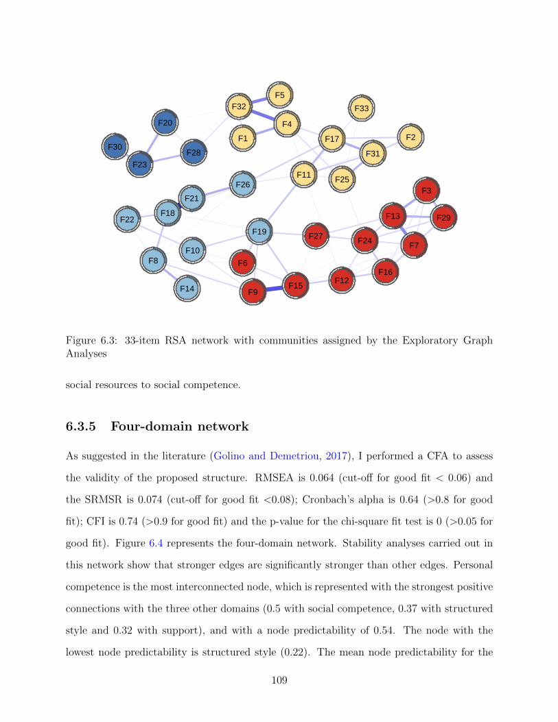
Figure 6.3: 33-item RSA network with communities assigned by the Exploratory GraphAnalyses

social resources to social competence.

6.3.5 Four-domain network

As suggested in the literature (Golino and Demetriou, 2017), I performed a CFA to assess

the validity of the proposed structure. RMSEA is 0.064 (cut-off for good fit < 0.06) and

the SRMSR is 0.074 (cut-off for good fit <0.08); Cronbach’s alpha is 0.64 (>0.8 for good

fit); CFI is 0.74 (>0.9 for good fit) and the p-value for the chi-square fit test is 0 (>0.05 for

good fit). Figure 6.4 represents the four-domain network. Stability analyses carried out in

this network show that stronger edges are significantly stronger than other edges. Personal

competence is the most interconnected node, which is represented with the strongest positive

connections with the three other domains (0.5 with social competence, 0.37 with structured

style and 0.32 with support), and with a node predictability of 0.54. The node with the

lowest node predictability is structured style (0.22). The mean node predictability for the

109

PersComp

Support

SocComp

Style

PersComp: Personal CompetenceSupport: SupportSocComp: Social CompetenceStyle: Structured Style

Figure 6.4: Four-domain network of resilience. Each node represents a domain as detectedby the Exploratory Graph Analysis.

four-domain network is 0.37. A negative edge is found between structured style and social

competence.

6.4 Discussion

This paper is to my knowledge the first work to report a network analysis of the psychological

construct of resilience as conceived in RSA. The different analyses carried out bring new

and interesting information on the construct, reporting overall that resilience is formed of

interacting components which are not mere consequences of a latent variable. If the network

structures presented in this work were to replicate in different samples, interventions to

improve protective factors in individuals may become more efficient by acting on meaningful

targets, such as two highly connected nodes in the resilience network.

The item network shows that the strongest edges are shared between items representing

overall the same aspect of a domain: such connections must therefore be interpreted as shared

variance between items, such as reported in recent papers that further address the issue (Fried

and Cramer, 2017) and propose solutions such as estimating a network of domains instead of

a network of items (Briganti et al., 2019). However, in the case of the RSA, the item network

110

sheds light on the connectivity between items from different subscales: items from the RSA

in my sample therefore form a complex system of mutual interactions that actively contribute

to the construct of resilience itself. From a network perspective, this means the observed

group is likely to similarly answer items that present a connection in the resilience network,

after controlling for all other items in the network (Briganti et al., 2018). Items from the RSA

also have different levels of importance in the network; this information is provided by node

predictability, which is an absolute measure of the interconnectedness of a node (Haslbeck

and Fried, 2017). In the item network, two nodes from the social competence domain (18

and 21) show the highest predictability, sharing over 50% of variance with surrounding nodes

in the network structure: however, as addressed in the section 3, the two nodes with the

highest node predictability are also the nodes sharing the strongest edge in the network; the

high predictability is therefore largely influenced by the presence of one very strong edge,

which is also a known feature influencing centrality criteria.

The six-domain network further helps us explore the connectivity and importance of the

protective factors as described in the most recent version of the RSA. Domains of the RSA

form a heterogenous system with positive and negative connection: this further supports the

theory that domains of resilience are not interchangeable measures of resilience; the construct

arises from the connections among domains. For instance, two negative connection exists, the

first between structured style and perception of self, and the second between family cohesion

and social competence. Negative edges are a rare finding when dealing with a network

approach of psychological constructs; a recent paper (Briganti et al., 2019) addressed the

issue of interpreting negative edges in the case of a domain network such as the six-domain

network of RSA estimated in this paper. From a theoretical point of view, I may interpret

the negative edge between social competence and family cohesion as follows: knowing that

an individual’s resilience is strongly drawn from the ability to rapidly adapt in different social

context, that individual’s resilience is less likely to be drawn from the support originating

from a cohesive family (and vice versa). The same line of reasoning applies to the negative

111

connection between structured style and perception of self: knowing that an individual’s

resilience is drawn from routines and structure, his/her resilience is less likely drawn from

confidence in own capabilities/decisions (and vice versa).

In the six-domain network, the strongest connections are found between social resources

and family cohesion, and between planned future and perception of self. As mentioned in

section 1, these two couples of domains theoretically overlap, with several items measuring

the same source of resilience; it is therefore not surprising that these domains are highly

connected in a network structure. Domains of resilience predict each other well, with mean

node predictability indicating 55% of shared variance on average. Planned future is the most

important node in the resilience network according to the node predictability estimates (it

has 67% of shared variance with surrounding nodes).

The EGA reported the existence of four communities in the item network, with a first

new community, personal competence, emerging from perception of self and planned future,

and a second new community, support, emerging from social resources and family cohesion.

Personal competence (adding up items from perception of self and planned future) is, from

a psychometric point of view, not a surprising finding: the two communities composing the

new domain were originally a single factor (Friborg et al., 2003). However, social resources

and family cohesion were originally proposed as distinct factors since the first published

version of the scale, which makes this analysis an interesting finding.

In the four-domain network, the new personal competence community is the most in-

terconnected node, sharing the three strongest connections in the network and 54% of its

variance with the three surrounding domains. A negative edge is found between structured

style and social competence, two domains unconnected in the six-domain network: from a

theoretical point of view, it is plausible to consider that in people whose resilience depends on

a structured life based on routines, being able to adapt in social situations is a less important

source of resilience, controlling for all other sources (and vice versa). On average, nodes in

the four-domain network are less predictable then domains in the six-domain network, with

112

37% of shared variance.

However, when comparing results from the CFA of both the six-factor model and the

four-factor model such as suggested in the literature (Golino and Demetriou, 2017), the

six-factor model presents with better indicators than the four-factor model. This being the

first network approach to this particular scale of resilience, future papers may endeavor to

replicate these findings in other samples while comparing the original six-factor structure

with structures proposed from EGA.

My analyses should be interpreted in the light of several limitations. First, my dataset

is composed of university students, which may likely limit the generalization of my findings

to different samples. Second, because this is a cross-sectional study, I cannot infer whether

a given node (item or domain) causes or is caused by another node to which it is connected;

determination of causality requires time-series which may be interesting in follow-up studies

of, for instance, young individuals with and without childhood adversities (Fritz et al., 2018).

113

Chapter 7

A network model of narcissism

Abstract

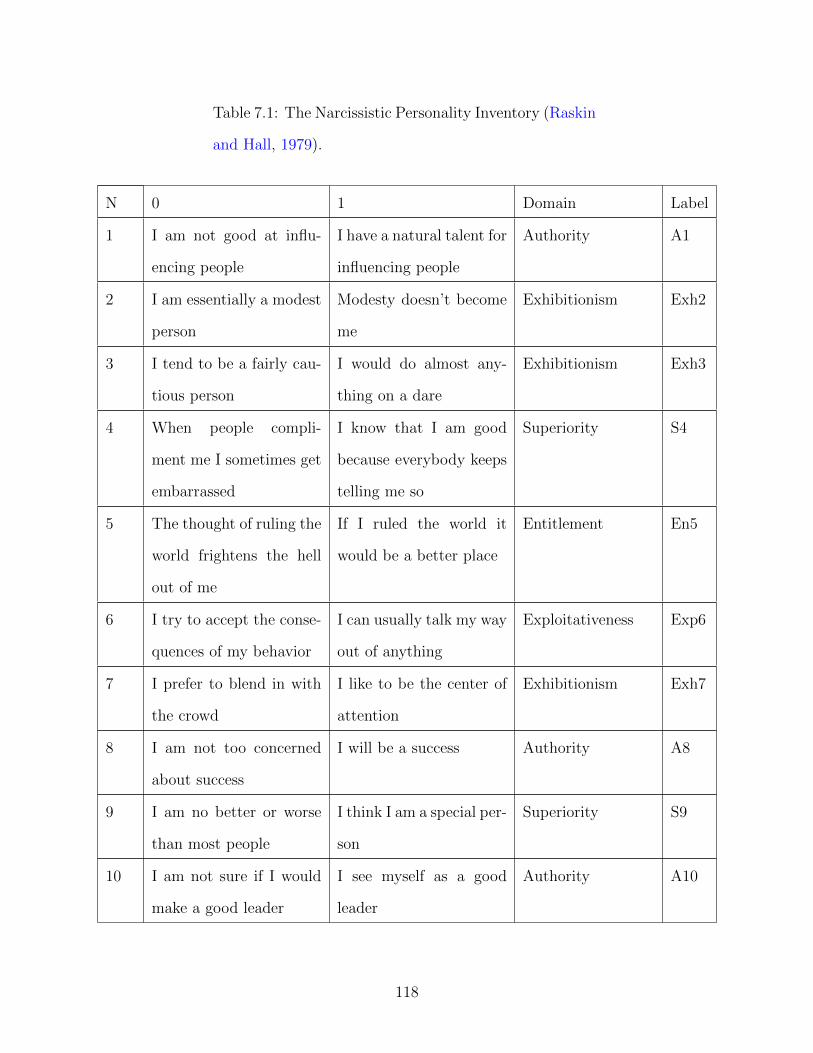
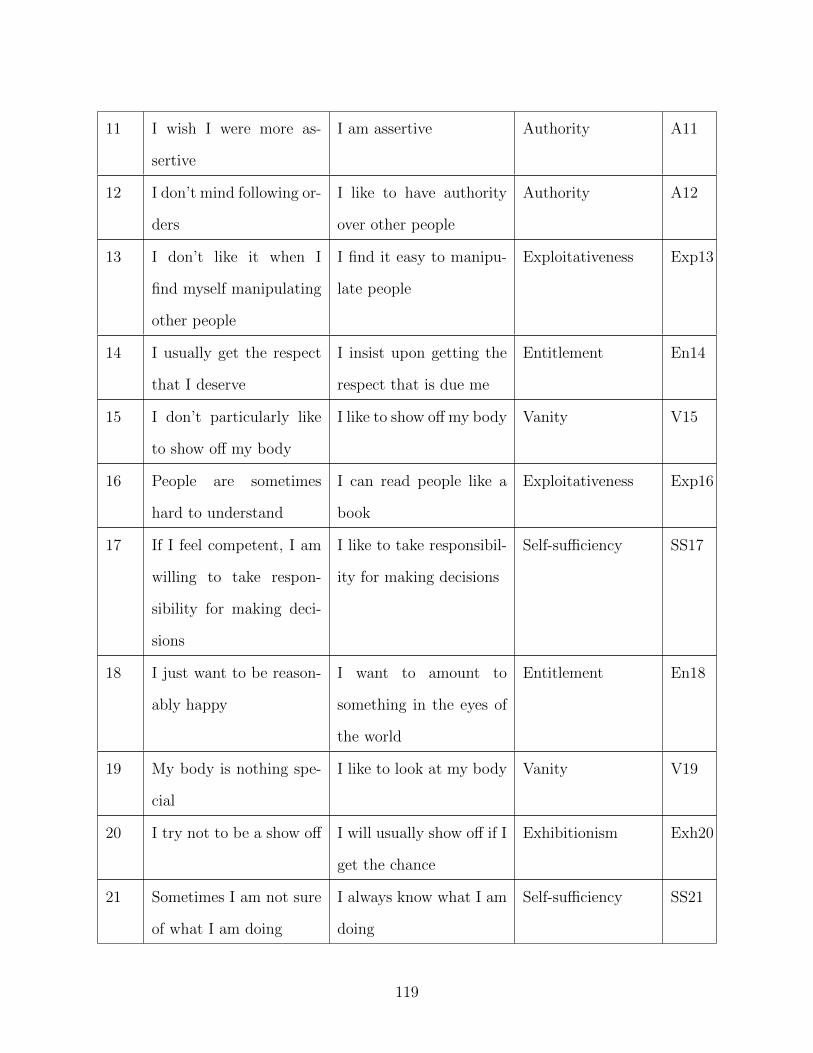
The aim of this work is to explore the Narcissistic Personality Inventory (NPI) using

network analysis in a dataset of 942 university students from the French-speaking part

of Belgium. I estimated an Ising Model for the forty items in the questionnaire and

explored item interconnectedness with strength centrality. The NPI is presented as

an overall positively connected network with items from entitlement, authority and

superiority reporting the highest centrality estimates. Network analysis highlights new

properties of items from the NPI. Future studies should endeavor to replicate my

findings in other samples, both clinical and non-clinical.

7.1 Introduction

Narcissism has been defined as the ability to maintain a positive self-image despite various

internal and external processes. Narcissistic subjects have a need for self-enhancing experi-

ences from their social environment (Pincus et al., 2009). Narcissism has been theorized to

possess both normal and pathological aspects, which have been considered by some authors

as two different personality constructs (Von Kanel et al., 2017) and as a continuum by oth-

ers (Paulhus, 1998). Grandiosity and vulnerability are considered as the two expressions of

114

narcissism (Cain et al., 2008): grandiose narcissism is associated with the predisposition to

exploit others, a lack of empathy and one’s feelings of entitlement and superiority, whether

vulnerable narcissism is associated with a depleted self-image, social withdrawal and suici-

dality (Miller et al., 2013). The current gold-standard models of narcissism, the trifurcated

model (Miller et al., 2016) and the narcissism spectrum model (Krizan and Herlache, 2018)

postulate that grandiosity and vulnerability are two largely independent factors that are tied

together by a core of entitlement.

The main tool used to study the construct of narcissism is the Narcissistic Personality

Inventory or NPI (Raskin and Hall, 1979), which represents grandiose narcissism (Krizan

and Herlache, 2018). The NPI consists of forty dichotomous items composed of both a

narcissistic and a non-narcissistic statement. The authors of the questionnaire propose seven

domains of narcissism: authority reflects one’s need for authority and success (e.g., item 33

“I would prefer to be a leader”); exhibitionism represents one’s need to be the center of

attention in a social context (e.g., item 30 “I like to be the center of attention”); superiority

measures one’s belief of being better than other people (e.g., item 40 “I am an extraordinary

person”); entitlement reflects one’s desire to receive respect and wield power (e.g., items 14

“I insist upon getting the respect that is due me” and 27 “I have a strong will to power”);

exploitativeness represents one’s capacity to manipulate other people (e.g., item 13 “I find it

easy to manipulate people”); self-sufficiency measures one’s autonomy and belief in oneself

(e.g., items 22 “I rarely depend on anyone else to get things done” and 34 “I am going to

be a great person”); vanity measures one’s admiration of one’s own physical appearance

(e.g., item 19 “I like to look at my body”). However, this seven-domain structure of the

NPI is controversial; several studies report different structures of the questionnaire, such as

a four-factor model (Emmons, 1987) and a three-factor model (Boldero et al., 2015).

Despite inconsistent results in the exploration of dimensionality (Ackerman et al., 2011;

Corry et al., 2008; Kubarych et al., 2004), narcissism is commonly understood as composed

of domains that are interchangeable measures of the construct proposed. In the last decade,

115

a new way of analyzing psychological constructs as complex systems has been proposed:

the network approach (Borsboom, 2017). Such complex systems are uncovered in empirical

studies with network models, that represent a given construct as emerging from mutual

interactions of its components (Borsboom and Cramer, 2013).

The network approach has been used to analyze a number of mental disorders, such as

depression (Mullarkey et al., 2018), posttraumatic stress disorder (Fried et al., 2018; Phillips

et al., 2018). Psychological constructs such as personality (Costantini et al., 2015), empathy

(Briganti et al., 2018) and self-worth (Briganti et al., 2019) have also been proposed as

network structures. The Pathological Narcissism Inventory has been recently investigated

through the lens of network analysis (Di Pierro et al., 2019), which identified Contingent self-

esteem, Grandiose Fantasies and Entitlement Rage to be important traits of the constructs.

A network can be composed of items of a questionnaire such as the NPI. In the case of a

network of self-reported questions, several items tend to be redundant and represent the

same aspect of a construct; this has been described in the network literature as a delicate

challenge, since the meaning of a connection between two redundant elements changes and

simply represent shared variance between the two corresponding questions that measure the

same thing (Fried and Cramer, 2017).

This challenge applies to the NPI: for instance, items 19 (“I like to look at my body”)

and 29 (“I like to look at myself in the mirror”) are two very similar measurements from

vanity. This is the case for several other items in the questionnaire, including items from

different domains, such as items 12 (“I like to have authority over other people”) and 27

(“I have a strong will to power”) that respectively belong to authority and entitlement. In

a network structure, I would expect these items to be strongly associated. It is plausible

to consider narcissism as a network of components (in this case, items from a self-reported

questionnaire indicating an individual’s perspective on narcissistic traits) that mutually in-

fluence each other instead of being passive consequences of the same construct. The network

approach to narcissism is relevant because it might allow in clinical samples the identification

116

of meaningful targets for intervention, even more so if considered that normal and patholog-

ical narcissism form a continuum. The aim of this work is to explore for the first time NPI

items and their relationship in a network of narcissism, therefore applying network analysis

to the items of the questionnaire. Network analysis has been shown to offer substantial in-

sight as a complementary tool to factor analysis, which is a more established technique in the

field of personality assessment (Briganti et al., 2018): as mentioned, modeling a construct or

mental disorder as a network can highlight connections between items or symptoms which

can therefore be used for intervention (Blanken et al., 2019). First, I want to explore the

connectivity of the NPI network. Second, I want to explore the importance of each item in

the questionnaire using strength centrality, which is the absolute sum of connections of a

given node in the network (Boccaletti et al., 2006).

7.2 Method

7.2.1 Participants

The data set used for this study is composed of 942 university students from the French-

speaking region of Belgium. The participants were first-year students in several Belgian

universities and in different undergraduate courses and they volunteered to fill a set of

questionnaires which included a French version of the NPI.

7.2.2 Measurement

The NPI (Table 7.1) contains 40 items that are meant to assess seven domains of narcis-

sism: authority, exhibitionism, superiority, entitlement, exploitativeness, self-sufficiency and

vanity. Items from different domains are shuffled in the questionnaire, and their scoring is

dichotomous: each item possesses both a narcissistic and a non-narcissistic statement. The

protocol of this study was approved by the Ethical Committee of the Erasme university

hospital.

117

Table 7.1: The Narcissistic Personality Inventory (Raskin

and Hall, 1979).

N 0 1 Domain Label

1 I am not good at influ-

encing people

I have a natural talent for

influencing people

Authority A1

2 I am essentially a modest

person

Modesty doesn’t become

me

Exhibitionism Exh2

3 I tend to be a fairly cau-

tious person

I would do almost any-

thing on a dare

Exhibitionism Exh3

4 When people compli-

ment me I sometimes get

embarrassed

I know that I am good

because everybody keeps

telling me so

Superiority S4

5 The thought of ruling the

world frightens the hell

out of me

If I ruled the world it

would be a better place

Entitlement En5

6 I try to accept the conse-

quences of my behavior

I can usually talk my way

out of anything

Exploitativeness Exp6

7 I prefer to blend in with

the crowd

I like to be the center of

attention

Exhibitionism Exh7

8 I am not too concerned

about success

I will be a success Authority A8

9 I am no better or worse

than most people

I think I am a special per-

son

Superiority S9

10 I am not sure if I would

make a good leader

I see myself as a good

leader

Authority A10

118

11 I wish I were more as-

sertive

I am assertive Authority A11

12 I don’t mind following or-

ders

I like to have authority

over other people

Authority A12

13 I don’t like it when I

find myself manipulating

other people

I find it easy to manipu-

late people


14 I usually get the respect

that I deserve

I insist upon getting the

respect that is due me

Entitlement En14

15 I don’t particularly like

to show off my body

I like to show off my body Vanity V15

16 People are sometimes

hard to understand

I can read people like a

book


17 If I feel competent, I am

willing to take respon-

sibility for making deci-

sions

I like to take responsibil-

ity for making decisions

Self-sufficiency SS17

18 I just want to be reason-

ably happy

I want to amount to

something in the eyes of

the world

Entitlement En18

19 My body is nothing spe-

cial

I like to look at my body Vanity V19

20 I try not to be a show off I will usually show off if I

get the chance

Exhibitionism Exh20

21 Sometimes I am not sure

of what I am doing

I always know what I am

doing


119

22 I sometimes depend on

people to get things done

I rarely depend on any-

one else to get things

done


23 Sometimes I tell good

stories

Everybody likes to hear

my stories


24 I like to do things for

other people

I expect a great deal from

other people

Entitlement En24

25 I take my satisfactions as

they come

I will never be satisfied

until I get all that I de-

serve

Entitlement En25

26 Compliments embarrass

me

I like to be complimented Superiority S26

27 Power for its own sake

doesn’t interest me

I have a strong will to

power

Entitlement En27

28 I don’t care about new

fads and fashions

I like to start new fads

and fashion

Exhibitionism Exh28

29 I am not particularly in-

terested in looking at my-

self

I like to look myself in the

mirror

Vanity V29

30 It makes me uncomfort-

able to be the center of

attention

I really like to be the cen-

ter of attention

Exhibitionism Exh30

31 People can’t always live

their lives in term of

what they want.

I can live my life in any

way I want to


120

32 Being an authority

doesn’t mean that much

to me

People always seem to

recognize my authority

Authority A32

33 It makes little difference

to me whether I am a

leader or not

I would prefer to be a

leader

Authority A33

34 I hope I am going to be

successful

I am going to be a great

person


35 People sometimes believe

what I tell them

I can make anybody be-

lieve anything I want

them to


36 Leadership is a quality

that takes a long time to

develop

I am a born leader Authority A36

37 I don’t like people to pry

into my life for any rea-

son

I wish somebody would

someday write my biog-

raphy

Superiority S37

38 I don’t mind blending

into the crowd when I go

out in public

I get upset when people

don’t notice how I look

when I go out in public

Exhibitionism Exh38

39 There is a lot that I can

learn from other people

I am more capable than

other people


40 I am much like every-

body else

I am an extraordinary

person

Superiority S40

121

7.3 Network analysis

The software R (open source, available at https://www.r-project.org/) was used to carry

out the analyses. I used the R-packages “qgraph” (Epskamp et al., 2012) and “glasso”

(Friedman et al., 2014b) and IsingFit (van Borkulo et al., 2014) for network estimation and

visualization, and “bootnet” (Epskamp and Fried, 2018) for stability analyses.

7.3.1 Network estimation

An Ising Model (IM) was estimated from my dataset. An IM (van Borkulo et al., 2014;

Marsman et al., 2018) is the binary equivalent of the Gaussian Graphical Model used for

continuous datasets (Epskamp and Fried, 2018). A lasso (least absolute shrinkage and se-

lection operator) was used to provide a conservative network structure (Epskamp and Fried,

2018). I used the default eLasso procedure which combines an l1-regularized logistic re-

gression with an Extended Bayesian Information Criterion or EBIC (Chen and Chen, 2008)

which reports relevant connections between variables. The lasso procedure provides a neigh-

borhood (set of nodes that interact) and decides the best set of regression coefficients given

the data, based on EBIC (which is in turn based on log likelihood); the set of regression

coefficients with the lowest EBIC is the best fit. To construct the final network, a connec-

tion is drawn between two nodes A and B if node A has node B in its set of neighbors and

vice-versa.

The default eLasso procedure was used in bootnet and IsingFit (van Borkulo et al.,

2014). The hyperparameter gamma (to select how many edges the model recovers) was set

by default at 0.25; the optimal tuning parameter lambda (used to select the model with

the best fit) was automatically chosen by the eLasso procedure. The network structure

resulting from this estimation contains items from the NPI represented as nodes. An edge

is a connection between two nodes in the network, which is interpreted as the existence of a

connection between two nodes controlling for all other nodes in the network.

122

While estimating a network structure from items of a questionnaire, a connection between

two nodes means that the observed group answers on average in a similar way to both items

of the questionnaire (Briganti et al., 2018). Each edge in the network represents either a

positive (visualized as blue edges) or a negative connection (visualized as red edges). The

thickness and color saturation of an edge denotes its weight (the strength of the connection

between two nodes). The Fruchterman-Reingold algorithm places the items in the network

based on the inverse of the sum of connections of a given node with other nodes (Fruchterman

and Reingold, 1991): this means that strongly connected nodes are put closer in the network

visualization.


I estimated strength centrality (Boccaletti et al., 2006) for the 40 items in the questionnaire.

Strength centrality represents the absolute sum of the edges of a given node and therefore

informs us of the connectedness of items in the network (Briganti et al., 2018).


Stability analyses (Epskamp and Fried, 2018) were carried out through bootstrapping, which

is a repeated estimation of a model under sampled data: I used 2000 bootstraps in this pa-

per. An edge weight difference test was performed to compare all edges against all other

edges and to answer the question “is edge A significantly stronger than edge B?”. Centrality

stability analyses for strength centrality were also carried out to answer the question “is the

centrality order stable?”. Centrality difference test was performed to answer the question

“is the centrality estimate of node A statistically different from that of node B?”. I used the

subsetting bootstrap procedure that re-estimates the network with a dropping percentage of

participants to determine the stability of centrality estimation, and results in a centrality-

stability coefficient (CS-coefficient) that should not be lower than 0.25 and preferably above

0.5. Both difference tests (edge weight and centrality) are carried out by estimating con-

123

fidence intervals around the difference of two elements A and B (which are bootstrapped

edge weights or bootstrapped centrality estimates, depending on the test): if 0 belongs in

the confidence interval then there is no difference between A and B.

7.4 Results

7.4.1 Participants

Participants were 17 to 25 years old (M=20 years, SD=1.7 years), 55% of them were female

and 45% were male. 25.4% of students studied engineering, 20% medicine, 17.7% economics,

11.3% sciences, 4.7% psychology and 2% law. The average NPI score of the participants of

this study was 13 (out of 40), and the standard deviation was 6.4.

7.4.2 Network of narcissism

Figure 7.1 illustrates the estimated network of the 40-item NPI. Overall, items from the

NPI form a positively connected network. The strongest connections in the network are

found between nodes belonging to the same domain of narcissism: for instance, item 10

(“I see myself as a good leader”) is strongly associated to item 33 (“I would prefer to be

a leader”) and both belong to the authority domain; item 7 (“I like to be the center of

attention”) presents the second strongest connection in the network to item 30 (“I really

like to be the center of attention”) and both belong to exhibitionism; item 9 (“I think

I am a special person”) shares the strongest edge of the network with item 40 (“I think

I am an extraordinary person”) and both belong to the superiority cluster. In the case

of these three connections, the items involved in an edge measure the same aspect of the

construct. Several connections are found between items belonging to different domains, and

I want to illustrate some of these connections. Domains superiority and self-sufficiency are

connected through items 9 (“I think I am a special person”) and 39 (“I am more capable than

other people”); domains authority and entitlement connect through items 12 (“I like to have

124

A1

Exh2

Exh3

S4

En5

Exp6

Exh7

A8

S9

A10

A11

A12

Exp13

En14

V15

Exp16

SS17

En18

V19Exh20

SS21SS22

Exp23

En24

En25

S26

En27

Exh28

V29

Exh30

SS31

A32

A33

SS34

Exp35

A36

S37

Exh38

SS39

S40

Figure 7.1: Network composed of the 40 items from the NPI (Table 7.1). Each item isrepresented by a node (1 to 40) and belongs to a different domain of the NPI (indicatedby a color code). The name of each node is composed as following: an abbreviation of thedomain to which the item belongs to followed by the item number.

125

●

●

●

●

●

●

●

●

●

●

●

●

●

●

●

●●

●

●

●

●

● ●

●

●

●

●

●

●

●

●

●

●

●

●●

●

●●

●

0 10 20 30 40

01

23

45

67

Index

grap

h1.c

$InD

egre

e

Figure 7.2: Strength centrality estimates for the 40 items of the NPI. The Y-axis repre-sents centrality indices (the higher the estimate the more central the item), and the X-axisrepresents the 40 NPI items.

authority over other people”) and 27 (“I have a strong will to power”); domains authority and

exploitativeness connect through items 1 (“I have a natural talent for influencing people”)

and 35 (“I can make anybody believe anything I want them to”). These domains also tend to

measure the same thing, even though belonging to different domains. Some small, negative

edge are also found in the network, such as the one between items 11 (“I am assertive”) and

24 (“I expect a great deal from other people”).


Figure 7.2 shows strength centrality estimates for the 40-item NPI. Item 27 from entitlement

(“I have a strong will to power”) presents the highest strength estimate, which means that

it is the most interconnected node in the network. Other strong items include item 33

from authority (“I would prefer to be a leader”) and item 40 from superiority (“I am an

extraordinary person”). Several items present with a strength centrality of 0, which means

that they are not connected with any item in the network.

126


The edge weight bootstrap shows relatively narrow CIs, which indicates a precise estimation

of the edge weights in the network. The edge-weight difference test performed shows that

stronger edges are significantly stronger than other edges in the network; however, edges

9-40 and 7-30 are not statistically different from each other, which means that, even though

edge 9-40 reports a stronger connection in the network, I cannot safely interpret it to be

statistically stronger than edge 7-30. Strength centrality stability analyses report that the

centrality order is relatively stable, with a centrality stability coefficient (CS-coefficient)

of 0.67. Strength centrality difference test reports that stronger centrality estimates are

significantly stronger than other estimates but are not significantly different from each other;

for instance, I cannot infer whether the centrality of item 27 is really stronger than that of

item 33. I obtained a CS-coefficient of 0.67, which indicates stable results.

7.5 Discussion

This study is to my knowledge the first application of network analysis to the NPI. Con-

nections are shown between narcissistic domains and shed light on how they interact. Items

from the NPI are overall positively connected and some items are more connected than

others. Most items from the NPI share some variance and are connected. However, some

items present weak connections with others; this means that some nodes are conditionally

independent of all other items in the network. Connections exist both between items from

the same domain and between items from domain, and stability analyses show that I can

safely interpret connections in this study.

Several strong connections between items from the NPI are found in the network. In

the case of the three connections between items 10-33, 7-30 and 9-40 belonging to the same

domains (respectively authority, exhibitionism and superiority) as described in the Results

section, the interpretation of an edge changes (Fried and Cramer, 2017), and the resulting

127

connection simply represents shared variance between the two questions (since they measure

the same thing). In some cases, items from different domains also tend to represent the same

construct, such as items 12 and 27 that connect authority and entitlement in the network.

These items can be considered as “bridge items”, since they can transfer information from

one domain to another and vice-versa; however, bridge items as the examples described in

the Results section also tend to represent the same aspect of narcissism.

Centrality analysis shows that items from entitlement, authority, and superiority present

the highest strength centrality estimates: that means that items from these domains connect

well to a greater number of nodes in the network, therefore identifying these 3 domains as

containing specific items that are important in this NPI network. From a network point

of view, it is also not surprising to find entitlement to contain central items, as this find-

ing supports my current gold standard models of narcissism, the trifucated model (Miller

et al., 2016) and the narcissism spectrum model (Krizan and Herlache, 2018) that describe

entitlement as a connection between grandiosity and vulnerability. My finding also supports

the recent network study of pathological narcissism (Di Pierro et al., 2019), which reported

high centrality values for Entitlement Rage. In the network approach, if the observed group

scores high on a highly central node, then the observed group is also more likely to score high

on a relevant number of nodes in the network. The identification of central items may help

in identifying potential targets for clinical intervention in people suffering from narcissism.

My findings should be interpreted in the light of several limitations. First, my dataset is

composed of university students, which limits the potential generalization of my findings to

different samples. Second, because this is a cross-sectional study, I cannot infer whether a

given node (item or domain) causes or is caused by another node to which it is connected.

Third, redundancy among items that measure the same thing is an important issue that

has yet to be solved in psychological networks of self-reported questionnaires; in the case

of the NPI network, several items can be considered as redundant, which would alter the

connectivity with other items (such as reported with strength centrality values).

128

Further studies may endeavor to replicate my findings in different samples, both non-

clinical and clinical, to identify central features of narcissism.

129

Chapter 8

A network model of alexithymia

without fantasizing

Abstract

The aim of this paper is to explore network structures of the Toronto Alexithymia

Scale (TAS) in a large sample of 1925 French-speaking Belgian university students

and compare results with previous studies from different samples and tools to identify

potential targets for clinical intervention. I estimated network models for the twenty

items of the TAS and for its three domains difficulty identifying feelings, difficulty de-

scribing feelings and externally-oriented thinking. I explored item connectivity through

node predictability (shared variance with other network components). I performed an

Exploratory Graph Analysis (EGA) to explore the dimensionality of my dataset and

compare results with the original three-factor model; because a different model was pro-

posed, I estimated an additional network structure on the new structure. Items from

the TAS connect both within and between domains. The three-domain network iden-

tifies difficulty describing feelings as the most connected domain. The EGA reported

that three items from externally-oriented thinking form a new domain, distraction. In

the new four-domain network, difficulty describing feelings remains the most intercon-

nected domain; however, two negative connections are found. My findings support the

130

relative importance of identifying and describing feelings as a meaningful target for

intervention.

8.1 Introduction

The construct of alexithymia has been around for more than half a century: it was named

from Greek meaning “lack of word for emotion” (Sifneos, 1972). Alexithymia is understood

as a personality construct with four main features: 1) difficulty identifying and distinguishing

emotions from bodily sensations; 2) difficulty describing and verbalizing emotions; 3) poverty

of fantasy life; and 4) externally-oriented thinking (Loas et al., 2017).

It is a subject of interest in psychiatric research so as to better understand the physi-

ological basis of mental disorders associated with emotions, such as mania, addiction and

depression. Extensive neuroimaging research has been conducted on alexithymia, report-

ing alterations in affective arousal to external stimuli, voluntary cognitive functioning; an

impaired activation of the insula during cognitive processes has indicated a potential over-

lap between alexithymia and other psychiatric disorders presenting with impaired empathy

such as psychopathy and autism (Moriguchi and Komaki, 2013). Because of such clinical

implications, some researchers recommend totranspose the concept of alexithymia to that of

“affective agnosia” (Lane et al., 2015). The Toronto Alexithymia Scale (TAS) is the most

commonly used measure of alexithymia in empirical research (Bagby et al., 1994) and is

composed of twenty items designed to assess three domains: difficulty identifying feelings

(e.g. item 1 “I am often confused about what emotion I am feeling”); difficulty describing

feelings (e.g. item 4 “It is difficult for me to find the right words for my feelings”), and

externally-oriented thinking (e.g. item 8 “I prefer to just let things happen rather than to

understand why they turned out that way”). These three domains as originally described

are to be interpreted as passive and interchangeable consequences of the construct itself, and

therefore are not active contributors to alexithymia (Van Bork et al., 2017).

131

In the last decade, network analysis has affirmed itself as new way of analyzing data

in psychiatry and psychology, which allows to conceive constructs or mental disorders as a

complex system of mutually influencing elements (Borsboom and Cramer, 2013). In this

framework, the unobserved interactions between psychological components (for instance

symptoms, or items from a questionnaire) are often computed as regularized partial cor-

relations (Epskamp and Fried, 2018). Network analysis has been used to explore several

mental disorders, such as posttraumatic stress disorder (Fried et al., 2018; Phillips et al.,

2018), depression (Mullarkey et al., 2018), and autism (Ruzzano et al., 2015), but also psy-

chological constructs such as empathy (Briganti et al., 2018), self-worth (Briganti et al.,

2019) and resilience (Fritz et al., 2018; Briganti and Linkowski, 2019b).

When considering a network model of a psychological construct (such as represented by

a given questionnaire), a known challenge is that of redundancy of items in addressing the

measure of the same aspect of a given construct. This may result in the case of an empirical

study in a network where redundant items share very strong connections whose meaning

is different (it represents shared variance rather than a true interaction between the two

components). A solution to address this problem is the estimation of a network model of

the domains of the construct instead of a network model of items (Briganti et al., 2019)

to facilitate the process of inference (e.g. identifying relevant interactions between network

components).

Network analysis is also useful to recover the true number of item communities (or fac-

tors) in a dataset; this can be achieved to the highly effective and reliable Exploratory Graph

Analysis or EGA (Golino and Demetriou, 2017); in this case, a confirmatory factor analysis

(CFA) is useful to authenticate the structure suggested by EGA, as suggested in a simula-

tion study (Golino and Epskamp, 2017). A recent empirical study (Briganti and Linkowski,

2019b) which applied the recommended EGA procedure showed that the problem of redun-

dancy in psychological networks is not exclusive to questionnaire items but can extend to

construct domains as well; community detections in psychological networks may therefore

132

also be useful to re-evaluate the construct themselves.

Network models of a construct such as alexithymia are particularly interesting to inte-

grate in clinical practice since relevant components may serve as targets for intervention

(Fried et al., 2018); in the case of alexithymia, finding and acting upon potentials tar-

gets is particularly interesting since it may attenuate the neurocognitive alterations that

have been described in the literature. The construct of alexithymia as represented by the

Bermond-Vorst Alexithymia Questionnaire (BVAQ) and the Toronto Structured Interview

for Alexithymia (TSIA) has already been explored through the lenses of network analysis

(Watters et al., 2016a,b); in the case of the TSIA whose factors closely resemble those of the

TAS, the domains difficulty identifying feelings and difficulty describing feelings formed one

community and provided the most connected items.

I therefore aim to extend the conceptual framework of psychological networks to the

construct of alexithymia as represented by the TAS. In this study, I want first to explore

alexithymia as both a network of items (as reported in the questionnaire) and domains.

Second, I want to apply EGA to recover the number of communities in the network, compare

the outcome with previous studies (Watters et al., 2016a,b), and authenticate the suggested

structure with CFA; if the result differs from the original three-domain structure, I want

to estimate the network of the structure proposed by the community detection. Third, I

want to explore the connectedness of items and domains with node predictability, which

statistically represent the shared variance of a given network component with surrounding

components (Haslbeck and Fried, 2017). These exploratory analyses may have meaningful

clinical implications and serve as basis for future replication studies to identify and act upon

potential clinical targets in people with alexithymia.

133

8.2 Method

8.3 Data set

My dataset is composed of 1925 university students from the French-speaking region of

Belgium. Subjects were 17 to 25 years old (M = 19 years; SD = 1.6 years); 58% of them

were women and 42% were men.

8.4 Measurement

The TAS (Table 8.1) is composed of 20 shuffled items that measure alexithymia in three

domains: difficulty identifying feelings, difficulty describing feelings and externally-oriented

thinking. The minimum score for each item is 1 (“I completely disagree”) and the maximum

score is 5 (“I completely agree”). The questionnaire contains reverse-scored items whose

score is reversed before data analysis (Table 8.1). The protocol for this study was approved

by the ethical committee of the Erasme teaching hospital.

Table 8.1: The Toronto Alexithymia Scale (Bagby et al.,

1994)

N Item Domain WC

1 I am often confused about what emotion I

am feeling

Difficulty identifying

feelings

1

2 It is difficult for me to find the right words

for my feelings

Difficulty describing

feelings

4

3 I have physical sensations that even doctors

don’t understand


feelings

1

4 I am able to describe my feelings easily (re-

versed)


feelings

4

134

5 I prefer to analyse problems rather than just

describe them (reversed)

Externally-oriented

thinking

3

6 When I am upset, I don’t know if I am sad,

frightened, or angry


feelings

1

7 I am often puzzled by sensations in my body Difficulty identifying

feelings

1

8 I prefer to just let things happen rather than

to understand why they turned out that way

Externally-oriented

thinking

3

9 I have feelings that I can’t quite identify Difficulty identifying

feelings

1

10 Being in touch with emotions is essential (re-

versed)

Externally-oriented

thinking

3

11 I find it hard to describe my feelings more Difficulty describing

feelings

4

12 People tell me to describe my feelings more Difficulty describing

feelings

4

13 I don’t know what’s going on inside me Difficulty identifying

feelings

1

14 I often don’t know why I am angry Difficulty identifying

feelings

1

15 I prefer talking to people about their daily

activities rather than their feelings

Externally-oriented

thinking

2

16 1 prefer to watch “light” entertainment

shows rather psychological dramas

Externally-oriented

thinking

2

17 It is difficult for me to reveal my innermost

feelings, even to close friends


feelings

4

135

18 I can feel close to someone, even in moments

of silence (reversed)

Externally-oriented

thinking

3

19 I find examination of my feelings useful in

solving personal problems (reversed)

Externally-oriented

thinking

3

20 Looking for hidden meanings in movies or

plays distracts from their enjoyment.

Externally-oriented

thinking

2


Software

I used the software R (open source, available at https://www.r-project.org/). Packages

and functions to carry out the analysis include qgraph (Epskamp et al., 2012), glasso (Fried-

man et al., 2014b) for network estimation and visualization, mgm (Haslbeck and Waldorp,

2016) for node predictability, EGA (Golino and Epskamp, 2017) and igraph (Csardi and Ne-

pusz, 2006) for community detection, lavaan (Rosseel, 2012) for CFA and bootnet (Epskamp

and Fried, 2018) for stability.

Item network

A correlation matrix was calculated for the 20 TAS items and used as input to estimate a

Gaussian Graphical Model (GGM) which is a regularized partial correlation network (Ep-

skamp and Fried, 2018). I regularized the parameters of the GGM with a graphical lasso

(least absolute shrinkage and selection operator). Although recent relevant discoveries in

the network field (Williams et al., 2019) showed that regularized partial correlation network

estimation may provide an anti-conservative network model, my regularized TAS network

model reports fewer edges (and is therefore easier to interpret) than the nonregularized

partial correlation network.

The item network is composed of nodes representing alexithymia questions from the

136


TAS, and each node is surrounded by a pie chart representing its predictability (shared

variance with surrounding nodes). The position of nodes in the network is determined by

the Fruchterman-Reingold algorithm (Fruchterman and Reingold, 1991), which runs on the

sum of connections that a given node has with other nodes. Nodes are connected through

edges, which are interpreted as an association between two components, controlling for all

other nodes in the network. In the alexithymia item network, if two nodes A and B are

connected, it means for instance that if the observed group scored high on A, then the

observed group is also more likely to score high on B and vice versa (Briganti et al., 2018).

Each edge in the network has a weight which is defined as the importance of association

between two nodes and is denoted by thickness and color saturation; edges can therefore

be positive (blue edges, denoting a positive association) or negative (red edges, denoting a

negative association). For this work, I lowered the lambda parameter (tuning parameter).

Three-domain network

To better explore the interactions between alexithymia domains from the TAS, I estimated

a factor model for the three domains and obtained factor scores to estimate a GGM and

therefore a domain network as described in recent empirical papers (Briganti et al., 2019;

Briganti and Linkowski, 2019b).

Network stability

To safely interpret results from network analysis several stability tests were performed as

recommended in the literature (Briganti et al., 2018; Epskamp and Fried, 2018). To answer

the question “are edge weights accurately estimated”, 95% confidence intervals (CI) were

estimated through bootstrapping (2000 bootstraps were used). To answer the question “is

edge A significantly stronger than edge B” I performed an edge weight difference test.

137

Network inference

Node predictability (Haslbeck and Fried, 2017) represents shared variance that a given node

has with surrounding nodes; it has been defined as the upper bound of controllability: if

one assumes that all edges for a given node are directed toward that node, then node pre-

dictability provides an estimate of how much influence one can have on that node via all

other nodes (Briganti et al., 2019). Node predictability was estimated for all nodes in the

item and domain network and is represented as a pie chart surrounding each node.

To detect the number of communities in my TAS dataset, an EGA was performed (Golino

and Epskamp, 2017), which uses the walktrap algorithm. The algorithm is based on the

principle that adjacent nodes tend to belong to the same community (Yang et al., 2016).

Following the methodology of a recent study (Briganti and Linkowski, 2019b) and because

I found a different number of dimensions than the original model, I estimated an additional

network structure based on the results from EGA.

Four-domain network

I used CFA to estimate a four-factor model in the data and used the scores to estimate an

additional GGM. Node predictability and stability analyses were also carried out.

8.5 Results

8.5.1 Item network

Figure 8.1 shows the 20-item alexithymia network. Nodes connect both within and between

communities. I will hereby detail some of the connections. Item 2 (“It is difficult for me to

find the right words for my feelings”) is highly connected to item 4 (“I am able to describe

my feelings easily”, reversed) and both belong to difficulty describing feelings. Item 3 (“I

have physical sensations that even doctors don’t understand”) shares a connection with item

7 (“I am often puzzled by sensations in my body”) and both belong to difficulty identifying

138

TAS1

TAS2 TAS3TAS4

TAS5

TAS6

TAS7

TAS8

TAS9

TAS10

TAS11

TAS12

TAS13

TAS14

TAS15

TAS16

TAS17

TAS18

TAS19

TAS20

Figure 8.1: 20-item alexithymia network. Each node represents an item from the TAS ques-tionnaire (Table 8.1). The pie chart surrounding each node represents node predictability.

feelings. In these two cases, items strongly resemble each other and are therefore redundant;

the meaning of edges in this case shifts and should be interpreted as shared variance. Item 1

(“I am often confused about what emotions I am feeling”) from difficulty identifying feelings

and 2 (“It is difficult for me to find the right words for my feelings”) from difficulty describing

feelings are also strongly connected. Item 8 (“I prefer to just let things happen rather than to

understand why they turned out that way”) from externally-oriented thinking is associated

with item 9 (“I have feelings that I can’t quite identify”) from difficulty identifying feelings.

Item 15 (“I prefer talking to people about their daily activities rather than their feelings”)

from externally-oriented thinking is associated with item 17 (“It is difficult for me to reveal

my innermost feelings, even to close friends”) from difficulty describing feelings. Items 15,

16 and 20 from externally-oriented thinking are detached from the rest of the items from the

same factor.

139

ID

DES

Think

ID: Difficulty identifying feelingsDES: Difficulty describing feelingsThink: Externally−oriented thinking

Figure 8.2: Three-domain network. Each node represents a domain from the TAS.

8.5.2 Three-domain network

Figure 8.2 illustrates the three-domain alexithymia network. The domain difficulty describing

feelings is connected to the two other domains difficulty identifying feelings and externally-

oriented thinking which share no connection with each other. The connection between

difficulty describing feelings and difficulty identifying feelings is stronger than the connection

between difficulty describing feelings and externally-oriented thinking.


Edges are overall accurately estimated in both the item network and the three-domain net-

work, and I can safely interpret stronger edges in both networks to be significantly stronger

than weaker edges.

140


Node predictability

In the item network, the most predictable node is item 2 (“It is difficult for me to find

the right words for my feelings”), which shares 54% of variance with surrounding nodes.

Item 2 belongs to difficulty describing feelings, which is also the most predictable domain

in the three-domain network and shares 72% of variance with the two other domains. The

least predictable node in the item network is item 18 (“I can feel close to someone, even

in moments of silence”) which belongs to externally-oriented thinking and shares only 8%

of variance with other nodes. In the three-domain network, the least predictable node is

externally-oriented thinking which shares 12% of variance with the two other domains. The

mean node predictability is 24% in the item network and 51% for the three-domain network.

In both networks, difficulty describing feelings shows the most connectivity and externally-

oriented thinking the least connectivity.

Community detection

Figure 8.3 shows the twenty-item TAS network with colors corresponding to the communities

as detected by the EGA. Four communities are reported by the EGA: a new community

emerges from items 15, 16 and 20 from externally-oriented thinking. I defined the new

community as distraction, and factor analyses for both the three-factor and the four-factor

model report comparable and satisfactory construct validity.

8.5.5 Four-domain network

Figure 8.4 shows the four-domain network. In the four-domain network, two strong edges

exist: the first shared between distraction and externally-oriented thinking, and the second

between difficulty identifying feelings and difficulty describing feelings. Distraction and dif-

ficulty describing feelings share a weaker connection, such as externally-oriented thinking

141

TAS1

TAS2 TAS3TAS4

TAS5

TAS6

TAS7

TAS8

TAS9

TAS10

TAS11

TAS12

TAS13

TAS14

TAS15

TAS16

TAS17

TAS18

TAS19

TAS20

Figure 8.3: Community detection through Exploratory Graph Analysis.

ID

DES

Think

DST

ID: Difficulty identifying feelingsDES: Difficulty describing feelingsThink: Externally−oriented thinkingDST: Distraction

Figure 8.4: Four-domain network. Blue edges represent positive connections, red edgesrepresent negative connections.

142

and difficulty identifying feelings. However, two weak negative connections are reported: the

first between difficulty identifying feelings and distraction and the second between externally-

oriented thinking and difficulty describing feelings. The highest node predictability (73%) is

reported by difficulty describing feelings, and externally-oriented thinking reports the lowest

node predictability (54%). The mean node predictability is 63%. Stability analyses show

that edges are accurately estimated and each edge in the network is significantly different

from other edges in the network.

8.6 Discussion

This is to my knowledge the first network analysis of the psychological construct of alex-

ithymia as conceived in the TAS with state-of-the-art methods. The different analyses carried

out bring new and interesting information on the construct and build on previous findings.

The TSA item network sheds light on the connectivity between items within the same domain

and items from different domains of alexithymia. Several items that are strongly connected

(for instance item 2,3,4 and 7), report a certain redundancy in measuring the same aspect of

alexithymia with other items; other items share meaningful mutual interactions while mea-

suring a different aspect of alexithymia. Items from the alexithymia questionnaire report

different levels of interconnectedness. The EGA reported the existence of four communities;

the domain externally-oriented thinking loses three of its items to a new component that I

defined as distraction.

Because of the redundancy issue and the difficulty on extracting meaningful clinical

implications from a network of items (Briganti and Linkowski, 2019b), I estimated network

models of three and four domains: these models help us better explore the connections

between different domains of the TAS. Difficulty describing feelings being the most connected

domain in both network models, it may become of interest for future longitudinal studies

associated with clinical interventions. From a three-domain network perspective, answers

143

of the observed group to items from difficulty describing feelings can help us better predict

answers to items from the two other domains, and vice versa.

In both models, the most interconnected domain shares the strongest connections with

difficulty identifying feelings, which has similar connectivity; this may be due to the strong

similarity between these two aspects of alexithymia, which have already been shown to

merge in a single community in other network studies (Watters et al., 2016a,b); in my

dataset however, the two domains remain separate, as shown by EGA. Future studies may

also endeavor to explore the relationship between these two domains in other samples, as

well as the evolution of their association when an intervention is carried out.

Externally-oriented thinking splits in two separate communities: this finding, along with

the small negative edges found in the four-domain network should however first be replicated

in other different samples before being considered as clinically meaningful. This study reports

meaningful, clinical implications even if carried out on university students, more so because

it can build on previous findings.

I found similar findings as well as differences with previous network models of alexithymia

measurement tools (Watters et al., 2016a,b). For instance, in my TAS network models,

difficulty describing feelings is the most interconnected domain and contains node 2, the most

interconnected item in the questionnaire; this constitutes a similarity with the previous TSIA

and BVAQ studies. However, this domain remains a separate community from difficulty

identifying feelings, which constitutes a difference with previous studies. Because of these

findings, I support the arguments made by the authors of previous alexithymia network

analyses in stating that in a clinical setting, priority should be given in intervening on affect

awareness to better identify and describe feelings. However, in my sample, because items

from externally-oriented thinking and the domain itself do not show particularly strong

connectivity (even so because the domain splits into two distinct communities in the EGA),

it should not be given a higher priority in intervention than other components of alexithymia;

future studies may endeavor to replicate and compare findings to further understand if it is

144

a viable clinical target or not.

My findings should be met with a number of limitations. First, my dataset is composed of

university students, which likely limits the generalization of my findings to different samples.

Second, because this is a cross-sectional study, I cannot infer causality from connections

between nodes; this can be obtained, for instance, with time-series analyses.

Network analysis is a powerful set of tools to explore alexithymia in both clinical and

nonclinical samples. Future studies should endeavor to replicate findings from different

measurement tools and also address clinical samples of individuals with psychopathology.

This may help to confirm targets for clinical interventions (such as highly connected nodes

from the domain networks) and respective outcome in different types of mental illness.

145

Chapter 9

A network model of alexithymia with

fantasizing

Abstract

The aim of this paper is to explore the network structures of alexithymia compo-

nents in a large sample of university students and compare results with relevant prior

literature. Undirected and directed network structures of items from the Bermond

Vorst Alexithymia Questionnaire form B are estimated with state of the art network

analysis and structure learning tools. Centrality estimates are used to address the

topic of item redundancy and select relevant alexithymia components to study. The

undirected network structure of alexithymia components reports new features with re-

spect to prior literature, and the directed network structures offers new insight on the

construct.

9.1 Introduction

Alexithymia is named from the Greek words “a”, “lexis”, and “thymos”, meaning “lack of

word for emotion” (Sifneos, 1972): initially, it was used to describe emotional deficiencies

in patients suffering from classic psychosomatic disorders and epilepsy; those patients were

146

unaware of their feelings and were unable to fantasize about their inner thoughts, feelings,

and attitudes. This personality construct has been described more than half a century ago

and is characterized by several key features: difficulty identifying, verbalizing and analyzing

emotions, poor fantasy life and poor insight (Loas et al., 2017); these features have been

found to be constant over time, in contrast to what was initially observed.

Alexithymia is considered a subject of interest in psychiatric research, because it allows

for a deeper understanding of the physiological basis of mental disorders that are associated

with emotions, such as bipolar disorder, addiction and depression (Briganti and Linkowski,

2019c). Important clinical implications include this construct, such as the potential overlap

between alexithymia and other psychiatric disorders that present with a lack of empathy,

such as psychopathy and autism, as reported by extensive neuroimaging research that has

been conduced on the topic (Moriguchi and Komaki, 2013). Some authors recommend to

transpose the construct of alexithymia to that of “affective agnosia” (Lane et al., 2015).

Several psychometric tools have been validated to measure the construct of alexithymia.

One of the most well-known and widespread tools is the Bermond Vorst Alexithymia Ques-

tionnaire (BVAQ, shortened to AQ in this manuscript) which describes the construct of

alexithymia as a composed of five domains (Vorst and Bermond, 2001): difficulty identifying

emotions, difficulty analyzing emotions, difficulty verbalizing emotions, lack of emotional

insight, and poverty of fantasy life. This last domain of alexithymia is what sets the AQ

apart from its main counterpart, the Toronto Alexithymia Scale (Bagby et al., 1994), since

the latter psychometric scale does not contain any items that reflect the difficulty in fan-

tasizing. The AQ has been defined as a reliable tool for the study of alexithymia, and it

has been heavily investigated with exploratory and confirmatory factor analyses in several

populations (de Vroege et al., 2018).

From an ontological point of view, alexithymia as represented by psychometric tools such

as the AQ, developed and validated through the lenses of factor analyses, is a common cause

that can be measured via the items in the questionnaire; those items are a reflection of a

147

given factor (such as poor fantasy life), and each factor is itself a consequence of the common

cause that is the personality construct at hand (“the latent variable“). Hence, the observable

variables (the items themselves) only represent passive and interchangeable elements of the

latent variable. However, previous work on alexithymia highlighted the opportunity that is

the study of relationships between observable variables as a complementary tool to factor

analysis (Watters et al., 2016a,b).

The study of relationships between observable variables is allowed by network analysis,

which is a new way of analyzing psychiatric constructs as complex systems arising from inter-

actions between symptoms or components (Borsboom and Cramer, 2013). Such systems are

conceived as networks of nodes (the variables themselves) and edges (undirected connections

among variables): often, the unobserved connection among items are computed as partial

correlations, either regularized (Epskamp and Fried, 2018) or non-regularized (Williams and

Mulder, 2019); the latter has been shown to be a good fit for psychological data, since it is

low dimensional (the number of subjects exceeds by far the number of variables) (Williams

et al., 2019).

Network analysis is becoming more and more established in the field of psychometrics

and has been used to explore several mental disorders, such as posttraumatic stress disorder

(Fried et al., 2018; Phillips et al., 2018), depression (Mullarkey et al., 2018), autism Ruzzano

et al. (2015) and also psychological constructs, such as empathy (Briganti et al., 2018), self-

worth (Briganti et al., 2019), resilience (Fritz et al., 2018; Briganti and Linkowski, 2019b),

and narcissism (Briganti and Linkowski, 2019a). Alexithymia has been analyzed three times

with network analysis, two with the Toronto Alexithymia Questionnaire variants (Briganti

and Linkowski, 2019c; Watters et al., 2016b) and the AQ (Watters et al., 2016a): all these

studied in depth the connections between the items from alexithymia scales as well as the

regrouping of variables in domains.

The modeling of network structures of constructs such as alexithymia is particularly

interesting to integrate in clinical practice, since relevant components may serve as targets

148

for clinical intervention (Fried et al., 2018); in the case of alexithymia, finding and acting upon

relevant components may attenuate the neurocognitive alterations that have been described

in the literature.

However, the identification of the central components of a construct is complicated be-

cause of the redundancy of items in questionnaires (Briganti and Linkowski, 2019d): the

more redundancy exists in a questionnaire, the more the redundant items will be heavily

connected, which in turn will boost their relative importance: this can be called “central-

ity corruption” (Briganti and Linkowski, 2019c). Several strategies have been proposed to

overcome redundancy, such as exploring networks of domains instead of networks of items

(Briganti et al., 2019) and topological overlap. The latter has been proposed as a way of

dropping (or regrouping) the items that repeat the same aspect of a construct as other items

in a scale (Fried and Cramer, 2017), but it has not been used experimentally to regroup

items from a psychometric tool.

Moreover, because of the clinical relevance of alexithymia, it would be useful to uncover

causal relationships (directed connections among items) between meaningful items in order to

gain further information on the nature of connections among them. Such causal relationships

can be identified with specific tools in network science, such as Directed Acyclic Graphs

(DAGs). DAGs are the foundation of probabilistic models such as Bayesian networks and

other machine learning approaches that are capable of learning the underlying causal graphs

from data (Moffa et al., 2017), compute and represent such relationships. DAGs are well

established at the crossroads of machine learning and network science literature (Scutari

and Denis, 2015) and have been previously used in empirical research to explore depression

(McNally et al., 2017) and psychosis (Moffa et al., 2017).

Inspired by recent works in the field of both structure learning and alexithymia, I aim

to explore several network structure of the AQ. First, I will estimate a partial correlation

network of items from the AQ and infer their relative importance with established measures

in the field (Briganti et al., 2018). Second, I will tackle the problem of centrality corruption

149

by reducing the network to a group of five items from the scale based on their belonging to

a given domain and their relative importance in the network. Third, I will apply a structure

learning algorithm to construct a DAG of the main alexithymia components and therefore

explore causal pathways.

9.2 Method

9.2.1 Data set

The data set is composed of 537 university students attending programs from academic

institutions in the French-Speaking region of Belgium. Subjects were 17 to 25 years old

(M=20 years; SD=1.7 years). 71% of students were women and 29% were men.

9.2.2 Measurement

The AQ (Vorst and Bermond, 2001) is composed of items assessing alexithymia in five

domains: difficulty identifying emotions, difficulty analyzing emotions, difficulty verbalizing

emotions, lack of emotional insight, and poverty of fantasy life. In this study, the form B

of the questionnaire, which is composed of 20 items, was used. The data set for this study

was anonymized before analysis, and the protocol for this study was approved by the ethical

committee of the Erasme teaching hospital.


Software and packages

I used the software R for statistical computing (version 3.6.1, open source, available at

https://www.r-project.org/). The package used to carry out the analysis include qgraph

(Epskamp et al., 2012) for the undirected network estimation and visualization, bootnet

150


(Epskamp and Fried, 2018) for stability analyses and bnlearn (Scutari, 2010) for DAG esti-

mation.

Partial correlation network

Estimation of the partial correlation network I estimated a Gaussian Graphical

Model (GGM), that is, a partial correlation network for the items in the AQ. The GGM is

calculated as the inverse-covariance matrix: it is a network that includes a set of nodes that

correspond to the alexithymia items in the AQ and a set of edges that connect the nodes in

the network. If two nodes are connected, that means they are conditionally dependent given

all other nodes in the network (i.e their partial correlation is nonzero).

In the network of alexithymia components, if two nodes A and B are connected, it means

for instance that if the observed group scored high on component A, then the observed group

is also more likely to score high on component B, and vice versa, controlling for other nodes

in the network (Briganti et al., 2018). Each edge in the network has a weight representing

the strength of association between two alexithymia components; edges can be positive (and

therefore represent a positive association) or negative (denoting a negative association). In

the network the edge weight is represented as a combined thickness and saturation of the

edge; positive edges are shown in blue, and negative edges in red. Nodes are placed in the

network by the Fruchterman-Reingold algorithm, based on the sum of the connections a

given node has with other nodes (Fruchterman and Reingold, 1991).

Network inference To find comparatively important items in the partial correlation net-

work, I used strength centrality, which represents the absolute sum of the edges that nodes

in the network share with other nodes (Boccaletti et al., 2006).

Network accuracy and stability Accuracy and stability analyses were carried out fol-

lowing state-of-the-art methods (Epskamp and Fried, 2018) that were applied in previous

empirical papers (Briganti et al., 2018).

151

Accuracy analyses were carried out to answer the question: “is edge X accurately esti-

mated?”; 95% confidence intervals (CI) were estimated through bootstrapping (i.e., repeated

re-sampling from the original dataset to re-estimate network parameters; 2000 bootstraps

were used). Edge weight difference tests were carried out to answer the question: “is edge

X significantly stronger than edge Y?”.

Stability analyses were carried out to answer the question “is the centrality order stable?”

with the same bootstrapping method. Centrality difference tests were carried out to answer

the question “is the centrality of node A significantly stronger than the centrality of node

B?”.

Topological overlap To address the important topic of redundancy (i.e., items in the

questionnaire measuring the same aspect of the construct of alexithymia), the approach

proposed by Fried and Cramer (Fried and Cramer, 2017) of topological overlap was used.

Because items from the same domain strongly resemble each other, the most central item

from each domain (i.e items reporting the highest strength centrality score) was selected to

represent the corresponding facet of the construct in a five-item network.

Five-item network structure A five-item network structure was constructed with the

same methods described in the section “Estimation of the partial correlation network”, and

it was studied with inference analysis (that is, strength centrality computation) as well as

stability and accuracy analyses.

Directed Acyclic Graphs

In Bayesian networks an edge may represent a causal pathway between two nodes. The

structure of a Bayesian network can be estimated using constraint-based algorithms, which

analyze conditional independence relations among the nodes in the network. Constraint-

based algorithms produce a network model that can be interpreted as a causal model even

from observational data, under assumptions that in clinical terms exclude confounding and

152

sampling bias. In this paper the PC-algorithm is used, which is a constraint-based algorithm

(Spirtes et al., 1993).

To estimate a network model, the PC-algorithm first estimates an undirected network

model in which all pairs of nodes are connected, then deletes edges between conditional

independent pairs of variables, and directs edges starting with v-structures (two disconnected

nodes causing a third node). The estimated network was investigated using stability analysis

through bootstrapping.

Afterwards, a network is reported with a minimum connection strength (% of fitted

networks in which a given connection appears) of 85 and a minimum connection direction

(% of fitted networks in which a given connection has a given direction) of 50. This resulting

network therefore reports connections that are presents in more than 85% of the fitted

networks. Moreover, these connections present a direction (for instance, from node A to node

B) which is found in more than half of the fitted networks resulting from the bootstrapping

procedure. By default, with the software I used all edges are represented as red, and their

strength are represented as a combination of thickness and color saturation in the edges.

9.3 Results

9.3.1 Partial correlation network

Central items in the AQ

The five items showing the highest strength centrality values in each of the five domains are

reported in table 9.1.

“Difficulty identifying emotions” is represented by item 22, “I rarely let myself go to

my imagination”; “difficulty analyzing emotions” is represented by item 30, “I think one

should stay in touch with one’s feelings” (reversed item); “difficulty verbalizing emotions”

is represented by item 26, “When I am upset by something, I tell others about how I feel”

153

Table 9.1: Central items from the Bermond Vorst Alexithymia QuestionnaireN Item Domain22 I rarely let myself go to my imagination. Difficulty Identifying Emotions26 When I am upset by something, I tell others

about how I feel.Difficulty Verbalizing Emotions

29 I often get upset by unexpected events. Poor Emotional Insight30 I think one should stay in touch with one’s

feelings.Difficulty Analyzing Emotions

33 When I’m tired of myself, I can’t know if I’msad, afraid, or unhappy.

Poor Fantasy

(reversed item); “lack of emotional insight” is represented by item 29, “I often get upset by

unexpected events” (reversed item), and “poverty of fantasy life” is represented by item 33,

“When I’m tired of myself, I can’t know if I’m sad, afraid, or unhappy”. Three of the five

items with the highest centrality in the AQ twenty-item network have reversed scores.

Partial correlation network structure

The five-item network is represented in figure 9.1. As opposite as most construct networks

reported in the literature (Briganti et al., 2018, 2019; Briganti and Linkowski, 2019b,a,c),

the AQ network is not overall positively connected, as it includes several positive as well as

negative edges. Some of the connections in the network are described in the following. The

domains “difficulty identifying emotions” and “poor fantasy” show a positive connection, as

well as the domains “difficulty verbalizing emotions” and “emotional insight”, “poor emo-

tional insight” and “difficulty analyzing emotions”, and “difficulty verbalizing emotions” and

“difficulty analyzing emotions”. The domains “poor emotional insight” and “poor fantasy”,

are negatively connected in the network.

Network inference

The centrality estimates for the five-item network are reported in figure 9.2. Item 33 from

the domain “poor fantasy” and item 29 from the domain “poor emotional insight” report

the highest strength centrality estimates.

154

A22

A26

A29

A30

A33

A22: Difficulty Identifying EmotionsA26: Difficulty Verbalizing EmotionsA29: Poor Emotional InsightA30: Difficulty Analyzing EmotionsA33: Poor Fantasy

Figure 9.1: Partial correlation network. Each item represents one of the five domains in theAQ. Blue connections represent positive edges, red connections represent negative edges.

155

●

●

●

●

●

Strength

−1.0 −0.5 0.0 0.5 1.0

A22

A26

A29

A30

A33

Figure 9.2: Strength centrality estimates for the five-item network. The x-axis reports thestandardized z-scores and the y-axis reports the corresponding item.

156

A22

A26

A29

A30

A33

A22: Difficulty Identifying EmotionsA26: Difficulty Verbalizing EmotionsA29: Poor Emotional InsightA30: Difficulty Analyzing EmotionsA33: Poor Fantasy

Figure 9.3: Directed Acyclic Graph of alexithymia components obtained with the constraint-based PC-algorithm. Relationships between nodes (arrows) can be understood as causalpathways under certain assumptions.


Edges are overall accurately estimated in both the five-item and twenty-item network. I can

safely interpret stronger edges to be significantly stronger than weaker edges in the network.

Centrality estimates of nodes 29 and 33 in the five-item network are not significantly different,

which means I cannot say which of the two items is the most central.

9.3.2 Directed Acyclic Graph

The DAG of alexithymia components is reported in figure 9.3. Item 29 from the domain

“poor emotional insight” has three incoming edges from “poor fantasy” (item 33), “difficulty

verbalizing emotions” (item 26) and “difficulty analyzing emotions” (item 30). Item 22 from

157

the domain “difficulty identifying emotions” has an outgoing edge to item 33 from the domain

“poor fantasy”.

9.4 Discussion

This is to my knowledge the first network analysis of alexithymia components that com-

bines the classic partial correlation network approach with the Bayesian network approach.

Several of the resulting analyses bring new and interesting information on the construct of

alexithymia.

The partial correlation network for the twenty-item AQ reports a structure with an

overall mixture of positive and negative connections among items. Because items from the

same domain tend to measure the same aspect of the construct of alexithymia (that is, the

domain they belong to), the solution of topological overlap is applied: the original twenty-

item network is translated to a network of the five items in the AQ that have the highest

centrality values in their respective domains and that are reported in table 9.1. In this work,

the exploratory analyses on the twenty-item network (representing the full questionnaire) was

important to highlight with network inference methods relevant alexithymia components so

as to analyze a more simple and non-redundant network structure.

The five-item network reports, similarly to the twenty-item network, a set of positive

and negative edges: alexithymia components therefore present a heterogeneous connectivity.

Items from domains “poor emotional insight”, “difficulty verbalizing emotions”, “difficulty

analyzing emotions” share a set of positive connections: this means that the average score

of the observed group on one of these three questions can be predicted based on the score

on the other two questions. The same phenomenon is observed with items representing

the domains “difficulty identifying emotions” and “poor fantasy”. However, “poor fantasy”

and “poor emotional insight” are negatively connected, which from an undirected network

perspective, can be interpreted as follows: given all other alexithymia components in the

158

network, if the average score on one component is high, I may expect that the average score

of the observed group on the other component is low, and vice versa. My findings differ

slightly in that respect from the recent work of Watters et al (Watters et al., 2016b), in

which the two domains sharing a negative connection are “difficulty identifying emotions”

and “poor fantasy”.

The inference analyses show that items 29 and 33 share a negative connection in the

five-item network and are also the two items with the highest centrality estimates. However,

stability analyses show how the two centrality indices are not statistically different from each

other, hence I cannot say whether item 29 (that reports the highest centrality estimate) is

really the most central item.

In this work, the study of the undirected interplay among relevant alexithymia compo-

nents was an important preliminary step before entering the realm of causal inference through

the lenses of Bayesian networks. The DAG structure derives from the constraint-based PC-

algorithm. Directed connections between alexithymia components can be interpreted as

causal pathways under assumptions that in clinical terms exclude confounding and sampling

bias. The DAG reports that “poor emotional insight”, the lack of ability to fantasize, is

essentially a consequence of a poor ability to fantasize, a difficulty in verbalizing emotions

and a difficulty in analyzing emotions.

The information from the undirected five-item network inference analyses and the Bayesian

network analyses can be combined to obtain some interesting insights. First, in the partial

correlation network, “poor emotional insight” has a high estimated centrality, and the overall

item connectivity to other items in the network can be interpreted as predictability. Second,

the DAG shows that all edges that item 29 shares with other nodes point towards “poor

emotional insight”, which means that not only is “poor emotional insight” is a highly “pre-

dictable” domain of alexithymia, but that it is also a highly “controllable” domain of the

construct. This notion can be interpreted as that the aspect of alexithymia that deals with

the lack of insight regarding emotional arousal can be controlled through other aspects of

159

the construct.

The two network models proposed in this paper present similarities as well as differences:

for instance, both the partial correlation network and the DAG share several edges between

the same nodes; however, some nodes that are connect in the partial correlation network

are not connected in the DAG. The reason is the different definitions of the two models: in

a DAG two nodes are not automatically connected when they share a common child node

(such as item 29), but they will be connected in the corresponding partial correlation network

because of the indirect dependence conditional on that child node.

My results must be interpreted in light of several limitations. First, my data set is com-

posed of university students, which may limit the generalization of my findings to different

samples. Second, DAG structures do not involve loops: if in a three-node network a com-

ponent A causes component B and a component C, component C cannot cause component

A (the structure is therefore acyclic). However, it is plausible to consider that in the case

of alexithymia components, certain items may activate each other in a loop. Third, causa-

tion may be inferred from a connection between two nodes in a DAG assuming there are

no confounding or sampling bias. Further studies may endeavor to replicate my findings of

network structures (both Bayesian and non-Bayesian) of alexithymia components in different

samples, both non-clinical and clinical.

160

Chapter 10

A network model of autistic traits

Abstract

The aim of this work is to explore the construct of autistic traits through the

lens of network analysis with recently introduced Bayesian methods. A conditional

dependence network structure was estimated from a data set composed of 649 university

students that completed an autistic traits questionnaire. The connectedness of the

network is also explored, as well as sex differences among female and male subjects

in regard to network connectivity.The strongest connections in the network are found

between items that measure similar autistic traits. Traits related to social skills are the

most interconnected items in the network. Sex differences are found between female and

male subjects. The Bayesian network analysis offers new insight on the connectivity

of autistic traits as well as confirms several findings in the autism literature.

10.1 Introduction

For the past two decades, there has been a growing interest in psychiatric research for the

classification and measurement of autistic traits (Volkmar et al., 2009). The Diagnostic and

Statistical Manual of Mental Disorders (DSM-V) has defined a framework for autistic traits:

the Autism Spectrum Disorder (ASD), that includes child autism, Kanner’s infantile autism,

161

high-functioning autism, and Asperger Syndrome.

To diagnose a patient with ASD as defined in the classification, the clinician must use

diagnostic criteria that associate persisting deficits in communication and social interactions

with narrow and repetitive behaviors, interests or activities. These two features manifest in

childhood, affect social, academic or professional functioning, and are not better explained by

an intellect developmental disorder or a global developmental delay (American Psychiatric

Association, 2013). Although initially considered as an abnormal condition, several works

have showed how the distribution of autistic traits across the population is continuous (Wing,

1988; Constantino and Todd, 2003), and people diagnosed with autism score at the extreme

end of the distribution when autistic traits are measured (Baron-Cohen, 2010).

The Autism-Spectrum Quotient (AQ) is a widely used self-administered questionnaire

that provides a quantified evaluation of the degree to which an adult with a normal intelli-

gence quotient presents with signs of ASD. This measurement tool assesses the respondent’s

behaviors, preferences and cognition based on five domains of autistic functioning: social

skill, attention switching, attention to detail, communication, and imagination; autistic traits

are considered when the respondent shows poor social skill, strong attention focus, excep-

tional attention to detail, poor communication and poor imagination (Baron-Cohen et al.,

2001). The AQ was translated in several languages, such as Italian (Ruta et al., 2012),

Dutch (Hoekstra et al., 2008), Chinese (Lau et al., 2013), Japanese (Wakabayashi et al.,

2006), Turkish (Kose et al., 2013), Polish (Pisula et al., 2013), and Persian (Mohammadi

et al., 2012), and French (Kempenaers et al., 2017), and its structural validity was studied

using exploratory and confirmatory factor analysis (EFA and CFA) in the different trans-

lations. Although initial evidence supporting the structural validity of AQ, several studies

reported doubts regarding the factorial aspects of the tool (Hoekstra et al., 2011; Hurst et al.,

2007), with multiple works not obtaining the five-factor original model to fit in student data

(Hoekstra et al., 2011; Kloosterman et al., 2011; Lau et al., 2013); most of which argued for

shorter versions of the questionnaire. An abridged ten-item version of the AQ was therefore

162

created including “red flag” items for autism screening in general practice (Allison et al.,

2012). Despite criticism, the AQ is the most commonly used measurement tool for autistic

traits detection and is widely cited in scientific research (Ruzich et al., 2015).

The AQ was conceived based on the assumption that autistic traits are measurable con-

sequences of an underlying cause – that is, ASD. There is growing evidence pointing towards

defects in neuronal migration and the consequent malformation and malfunction of various

brain circuits as etiology of several brain disorders such as ASD (Pan et al., 2019), which

then presents itself through several autistic traits; as understood in the latent variable model

of mental illness, however, autistic traits do not actively participate to the clinical manifesta-

tion in subjects, as they are effects of the construct they stem from. Recent works, however,

have shown how behaviors in the autism spectrum reinforce each other (i.e. present a mutual

influence): learning strategies can therefore be adopted as to correct the social behavior of

people with autistic traits, and brain responses to social stimuli can be altered, especially

if an early intervention is conducted (Schuetze et al., 2017). From an ontological point of

view, this changes the attribute of autistic traits, that evolve from measurable consequences

of ASD to participate in its clinical presentation.

In the last decade, network analysis has affirmed itself as a new way of analyzing data in

psychiatry and psychology, which allows the conception of of mental disorders or constructs

as emerging from a complex system of mutually influencing components (Borsboom and

Cramer, 2013). This novel theoretical and methodological approach has been widely used

to explore a variety of constructs including depression (Mullarkey et al., 2018), obsessive

compulsive disorder (McNally et al., 2017), empathy (Briganti et al., 2018), personality

(Costantini et al., 2015), alexithymia (Briganti and Linkowski, 2019c), self-worth (Briganti

et al., 2019), posttraumatic stress disorder (Fried et al., 2018; Phillips et al., 2018), resilience

(Fritz et al., 2018; Briganti and Linkowski, 2019b), and narcissism (Di Pierro et al., 2019;

Briganti and Linkowski, 2019a).

Researchers usually analyze mental disorders and constructs as network composed of

163

items – answers of the observed group to a given questionnaire, such as the AQ. Conceiving

mental disorders as networks is interesting in clinical practice, since relevant components

in the proposed model could serve as a target for intervention (Fried et al., 2018). Most

of the recent empirical works using network analysis compute the unobserved interactions

between psychological components as regularized partial correlations (Epskamp and Fried,

2018): this is commonly achieved with `1-regularization (Friedman et al., 2014b), which

is also known as the “least absolute shrinkage and selection operator” or “lasso”, which

pushes the smaller estimates in the network structure to zero and therefore renders a sparse

(or conservative) network. The dominant lasso procedure used in network papers is the

graphical lasso that associates the `1-regularization with an Extended Bayesian Information

Criterion to determine a tuning parameter for the Gaussian Graphical Model (i.e. the

network) λ (Chen and Chen, 2008). However, recent work (see for example Williams et al.,

2019) reported how the regularization of network estimates can be inconsistent for model

selection, and does not provide evidence for the null hypothesis (i.e. evidence for no effect);

the latter consequence is of great importance because one of the core ideas of estimating

network structure is to uncover the conditional independence structure of a construct, and

therefore zero partial correlations among the variables composing the network.

Recently, Bayesian methodology has been introduced for the estimation of network struc-

tures. This new methodological framework allows for the estimation of Gaussian Graphical

Models with posterior probabilities that can assess the conditional dependent and indepen-

dent relations among components of a network with a decision rule that can be calibrated to

a desired level of specificity (Williams, 2018a). The Bayesian approach to the estimation of

network structures shows advantages when determining conditional independence relations

based on a network estimation where the threshold for selection depends on Bayes factors

(Williams and Mulder, 2019): this technique allows for studying the amount of evidence for

no effect in a given structure, which is useful to assess the uncertainty of estimates. Despite

offering such advantages, Bayesian methodology for the estimation of Gaussian Graphical

164

Models has never been used in empirical works concerning network analysis in psychological

or psychiatric research.

Inspired by these new advances in network analysis that has been applied in many fields

of psychiatry and psychology, I apply the network methodology to autistic traits. The aim of

the present work is therefore to perform a network analysis of the autistic traits as presented

in the 50-item version of the AQ with the Bayesian inference methods that have been recently

introduced (Williams, 2018a), in a sample of 649 university students.

Autism has recently been analyzed through the lens of network analysis in relationship

with depression (van Heijst et al., 2019); however, to my knowledge, this is the first time

that the AQ in its full 50-item version is explored with the network methodology, therefore

expanding this conceptual and methodological framework to the construct of autistic traits.

In this work, I will first estimate the conditional dependence structure of the autistic traits

network. Second, I will estimate node predictability, i.e. point-estimate and confidence

intervals for variance explained in all items, to measure their overall connectedness to other

items in the questionnaire. Third, I will explore sex differences among female and male

subjects from this study. The protocol for this study was approved by the ethical committee

of Hopital Erasme (Erasme Teaching Hospital) in Brussels, Belgium.

10.2 Method

10.2.1 Data set

My data set is composed of 649 university students from the French-speaking region of

Belgium. Subjects were 17 to 25 years old (M = 19.3, SD= ± 1.49); 58% were female and

42% were male.

165

10.2.2 Measurement

The AQ is composed of 50 items that assess autistic traits based on five domains: social skill,

attention switching, attention to detail, communication, and imagination. The minimum

score for each item is 1 (“Definitely disagree”) and the maximum score is 4 (“Definitely

agree”); approximately half of the items in the questionnaire are to be reverse-scored (Baron-

Cohen et al., 2001).


Software and packages

I used the software R for statistical computing (open source, available at https://www.

r-project.org/). The package used to carry out the analysis is BGGM (Williams and

Mulder, 2019).

Network estimation

I estimated a Gaussian Graphical Model (GGM) with Bayesian methods (Williams, 2018a),

that is, a partial correlation network for the 50 items in the AQ. The GGM is calculated as

the inverse-covariance matrix: it is a network that includes a set of nodes that correspond

to the autistic traits in the AQ and a set of edges that connect the nodes in the network. If

two nodes are connected, that means they are conditionally dependent given all other nodes

in the network (i.e their partial correlation is nonzero). In the network of autistic traits, if

two nodes A and B are connected, it means for instance that if the observed group scored

high on trait A, then the observed group is also more likely to score high on trait B, and

vice versa, controlling for other nodes in the network (Briganti et al., 2018). Each edge

in the network has a weight representing the strength of association between two autistic

traits; edges can be positive (and therefore represent a positive association) or negative

(denoting a negative association). The estimation of network with Bayesian methods allows

166



for providing evidence for the hypothesis that best predicts the observed data. For instance,

when testing for conditional dependence relationships among nodes, providing a Bayes Factor

(BF) between 3 and 20 as a cut-off value is associated with positive evidence, while a BF >

20 is associated with strong evidence (Kass and Raftery, 1995). For the network estimation

in this paper, a BF of 20 was used.

Node predictability and sex differences

I computed Bayesian R2 for the fifty autistic traits in the network, which represents the

percentage of variance explained of a given autistic trait with all other autistic traits in the

network (Williams and Mulder, 2019): this measure is commonly defined “node predictabil-

ity” in the network literature (Haslbeck and Fried, 2017) as it can be interpreted as how

well a node connects to other nodes in the network, or the self-determination of the network.

Node predictability can be understood as the upper bound of controllability: if one assumes

that all edges for a given node are directed toward that node, predictability provides an

estimate of how much influence I can have on the given node via all other nodes (Briganti

et al., 2019). Because the estimation of node predictability results in a distribution, I com-

pared the predictability estimates of females and male subjects in my data set to detect sex

differences in the network structures.

10.3 Results

10.3.1 Partial correlation network

The autistic traits partial correlation network is reported in figure 10.1. The strongest

connections are found between items that measure the same (or similar) autistic traits: for

example item 38 (“I am good at social chit-chat”, reversed) is strongly connected to item 17

(“I enjoy social chit-chat”, reversed) and item 26 (“I frequently find that I don’t know how

to keep a conversation going“). Two other examples of this phenomenon can be found in

167

1 23

4

5

6

7

8

9

10

11

12

13

14

15

16

17

18

19

20

21

22

2324

25262728

29

30

31

32

33

34

35

36

37

38

39

40

41

42

43

44

45

46

47

4849

50

Figure 10.1: Autistic traits (N = 649) partial correlation network with the 50 items from theAQ. Each edge (connection between nodes) is denoted by a weight represented by thicknessand color saturation.

168

the connections between item 8 (“When I’m reading a story, I can easily imagine what the

characters might look like”, reversed) and 20 (“When I’m reading a story, I find it difficult to

work out the characters’ intentions”) as well as between item 9 (“I am fascinated by dates”)

and 19 (“I am fascinated by numbers”).

However, connections between items that measure different autistic traits can also be

found in the network: for instance, 27 (“I find it easy to read between the lines when

someone is talking to me”, reversed) and 36 (“I find it easy to work out what someone

is thinking or feeling just by looking at their face”, reversed), 11 (“I find social situations

easy”, reversed) and 38 (“I am good at social chit-chat”, reversed), 35 (“I am often the last

to understand the point of a joke”) and 46 (“New situations make me anxious“).

Several negative connections can also be found in the network, such as the ones between

items 18 (“When I talk, it isn’t always easy for others to get a word in edgeways”) and

32 (“I find it easy to do more than one thing at once”, reversed), 21 (“I don’t particularly

enjoy reading fiction”, reversed) and 49 (“I am not very good at remembering people’s date

of birth”, reversed), 12 (“I tend to notice details that others do not”, reversed) and 31 (“I

know how to tell if someone listening to me is getting bored”).

10.3.2 Node predictability

The computed values for node predictability in the network are reported in figure 10.2. Item

38 (“I am good at social chit-chat”, reversed) has the highest R2 score (54%) in the network,

while item 41 (“I like to collect information about categories of things”) has the lowest R2

score (9%) in the network. The average R2 score is 20%.

10.3.3 Sex differences

Figure 10.3 represents sex differences in node predictability. The autistic trait network struc-

tures are statistically different in female and male subjects, with a Kullback-Leibler diver-

gence value (that translates the difference between the two node predictability distributions)

169

●

●

●

●

●

●

●

●

●

●

●

●

●

●

●

●

●

●

●

●

●

●

●

●

●

●

●

●

●

●

●

●

●

●

●

●

●

●

●

●

●

●

●

●

●

●

●

●

●

●

4124484

154237133

1623311

33352843467

50342040212

1130271429106

39228

442532185

453649129

1947261738

0.2 0.4 0.6bayes_R2

Nod

epost.pred

Figure 10.2: Node predictability (Bayesian R2) for the 50 nodes in the partial correlationnetwork.

●Yg1 vs Yg2

4.0 4.5 5.0 5.5Predictive Check

Con

tras

t

Figure 10.3: Sex differences in the network of autistic traits.

170

5049484746454443424140393837363534333231302928272625242322212019181716151413121110987654321

1 2 3 4 5 6 7 8 9 10 11 12 13 14 15 16 17 18 19 20 21 22 23 24 25 26 27 28 29 30 31 32 33 34 35 36 37 38 39 40 41 42 43 44 45 46 47 48 49 50Alternative Hypothesis Matrix

1.10

5.57log(BF)

Figure 10.4: Heat map reporting the edges that are statistically different in regard to thesex of participants. The darker the color, the higher the evidence.

of 5.8, and a p-value of 0.

A heat map is reproduced in figure 10.4 that represents which specific edges are different

in the female and male network structure (and the respective amount of evidence supporting

the difference, represented by a variation in BF). For instance, there is a moderate amount

of evidence supporting sex differences for the specific edges between items 14 (“I find making

up stories easy”) and 22 (“I find it hard to make new friends“), with a Bayes Factor of 115,

item 17 (“I enjoy social chit-chat”) and 34 (“I enjoy doing things spontaneously”), with a

Bayes Factor of 90.

The number of edges that are statistically different in regard to the sex of participants

variates among the items in the AQ and are reported in figure 10.5. Item 17 (“I enjoy social

chit-chat”) presents the highest number of edges in that regard.

171

●

● ●

● ● ●

● ●

●

● ●

●

●

●

● ●

●

●

●

●

●

● ●

●

●

●

● ●

●

●

●

●

● ●

● ●

●

●

●

●

●

●

●

● ● ●

●

●

●

●

0

1

2

3

4

1 2 3 4 5 6 7 8 9 10 11 12 13 14 15 16 17 18 19 20 21 22 23 24 25 26 27 28 29 30 31 32 33 34 35 36 37 38 39 40 41 42 43 44 45 46 47 48 49 50Item

Diff

eren

ces

Figure 10.5: Plot reporting for each node the number of edges that are statistically differentin regard to the sex of participants.

172

10.4 Discussion

This is the first work tackling the exploration of autistic traits through the lenses of Bayesian

network analysis and using the full 50-item version of the largely validated AQ (Baron-Cohen

et al., 2001). New methods introduced in recent Bayesian network literature (Williams,

2018a) allow for the estimation of conditional relationships among nodes with Bayesian

methods, including adopting a cut-off value to provide consistent evidence of the existence

of such relationships. Studying how items from the AQ connect sheds new information

on the important construct such as the one representing autistic traits. Even in a student

sample, investigating autistic traits through the lenses of network analysis is relevant because

“non-autistic” individuals may still present autistic traits, which are continuously distributed

across the general population.

The strongest connections in the network are found between items that measure similar

autistic traits: this is a recurrent phenomenon in network analysis of psychometric scales

(Briganti et al., 2018, 2019; Briganti and Linkowski, 2019b,a), which substantially influences

the network predictability.

Additional insight to the construct is mostly brought by connections between items that

measure different autistic traits, which are also found in the network, but their connection

strength is proportionally lower. From a network perspective, a connection between different

autistic traits such as the one between item 35 (“I am often the last to understand the point

of a joke”) and 46 (“New situations make me anxious”) is interesting if interpreted on a

clinical level. For instance, if a patient with autistic traits is bothered that he often lacks

the ability to understand jokes, it might be interesting for the clinician to investigate if and

how new situations make that same patient anxious, while taking into account other autistic

traits.

The presence of several negative connections in the network of autistic traits is an inter-

esting finding: the model is not overall positively connected, which is unusual from a latent

variable model perspective in which all items are considered as interchangeable measures of

173

the latent variable (in this case, the autism spectrum). This means several autistic traits

are inversely correlated. Negative connections occur between items from different domains

(i.e. different facets of the autism spectrum). For instance and in my sample, the average

individual presenting the autistic trait of being good at remembering people’s date of birth

(item 49) is less likely to present the autistic trait of enjoying reading fiction (item 21).

The highest R2 score in the network belongs to item 38, which measures an autistic

trait related to social skills. From a network point of view this can be interpreted as the

social skills trait being the domain that best predicts (or is predicted by) the rest of autistic

traits, since it is the most interconnected trait. On the other hand, item 41, an autistic trait

related to the domain of imagination, has the lowest R2 score in the network, which means it

is poorly connected to other autistic traits. The average R2 score is 20%, which means that

on average, nodes in the network of autistic traits share 20% of variance with other nodes.

Sex differences are found between the network of female and male subjects. This finding

supports extensive research done in the past few years which points to high AQ scores being

preponderant in male subjects (Ferri et al., 2018; Baron-Cohen et al., 2014); this study

however reports a difference in network connectivity, which is an additional information

never explored before.

My findings must be interpreted in light of certain limitations: two of them are hereby

described. First, the data set used in this study is composed of Belgian university students,

which likely limits the replicability of my findings in other sample, including samples with

people diagnosed with autism. Second, the uncertainty regarding the true network structure

of autistic traits must be taken into account: whereas it is possible to detect edges (non-zero

effects) with large uncertainty, inferring null effects (zero effects or the lack of connection

between two nodes) requires a much greater sample, especially in my case, where 50 items

are analyzed.

Further studies may endeavor to replicate my findings in other samples, including people

diagnosed with autism.

174

Part III

A network approach to mental

disorders

175

Chapter 11

A network model of depressive

symptoms in a student sample

Abstract

The Self-rating Depression Scale (SDS) is a psychometric tool composed of 20 items

used to assess depression symptoms. The aim of this work is to perform a network

analysis of this scale in a large sample composed of 1090 French-speaking Belgian uni-

versity students. I estimated a regularized partial correlation network and a Directed

Acyclic Graph for the 20 items of the questionnaire. Node predictability (shared vari-

ance with surrounding nodes in the network) was used to assess the connectivity of

items. The network comparison test was performed to compare networks from female

and male students. The network composed of items from the SDS is overall positively

connected, although node connectivity varies. Item 11 (“My mind is as clear as it used

to be”) is the most interconnected item. Networks from female and male students did

not differ. DAG reported directed edges among items. Network analysis is a useful tool

to explore depression symptoms and offers new insight as to how they interact. Further

studies may endeavor to replicate my findings in different samples, including clinical

samples to replicate the network structures and determine possible viable targets for

clinical intervention.

176

11.1 Introduction

Depression (also known as Major Depressive Disorder, MDD) is a common psychiatric disor-

der (Goldberg, 2011), and the top cause of disability worldwide (Lopez et al., 2006). In the

fifth edition of the Diagnostic and Statistical Manual of Mental Disorders or DSM (American

Psychiatric Association, 2013), depression is characterized as a combination of five symptoms

in a list of nine, including depressed mood or anhedonia (this symptom must be included in

each combination), increase or decrease in weight or appetite, fatigue, sleep problems and

suicidal ideation. Depression is then defined as a heterogenous disorder, which leads to an

important symptom variability (Fried and Nesse, 2015).

In most depression scales, such as the Hamilton Rating Scale for Depression (HRSD),

sum scores are used to explain the severity of the disorder (Hamilton, 1960). Zung created

in 1965 a self-rating depression scale (SDS) using 20 items representing symptoms from

three conceptual domains (Zung, 1965): pervasive effects (e.g. item 1: “I feel downhearted

and blue”), physiological equivalents (e.g. item 4: I have trouble sleeping at night”) and

psychological equivalents (e.g. item 19: “I feel that others would be better off if I were

dead”). In both these approaches, symptoms are considered as interchangeable measures of

depression.

In recent years, the network approach to psychopathology has been proposed as a novel

way of analyzing mental disorders as complex systems. This approach considers that a men-

tal disorder arises from connections among its symptoms, that can cause each other (Bors-

boom, 2017): this conceptualization differs from the latent variable theory, which states that

symptoms are passive consequences of an underlying cause. In psychiatry, the latter is un-

likely to identify a specific mechanism that causes a mental disease (Borsboom, 2008), which

makes the network approach an interesting alternative. Five principles of network theory

proposed by Borsboom are likely to apply in the case of depression: complexity (mental

disorders are characterized as interactions between the components of a network, such as

symptoms), symptom-component correspondence (components in a network are problems

177

defined as symptoms), direct causal connections (symptoms cause each other in a network),

network structure of mental disorders (certain symptoms are more connected than others

and symptoms from the same network often arise together) and hysteresis (symptoms acti-

vate each other even after the trigger cause has disappeared). Hysteresis has been proven

to be a dynamic present in depression (Cramer et al., 2016): a dormant (asymptomatic)

network of depression is present in the healthy individual: a trigger cause may activate one

or more symptoms which, in turn, activate the rest of the network in a “pathological” con-

dition. Mental health can then be defined as a stable state of a weakly connected network

(Borsboom, 2017).

Network analysis is a set of statistical techniques developed in the conceptual framework

of network theory to identify network structures in datasets. Network analysis has been

used in various fields, such as empathy (Briganti et al., 2018), posttraumatic stress disorder

(Fried et al., 2018), schizophrenia (Galderisi et al., 2018) and self-worth (Briganti et al.,

2019). Depression symptoms have already been analyzed with network analysis and several

networks structures have been proposed in the literature (Beard et al., 2016; McNally et al.,

2017).

Researchers usually analyze constructs as undirected networks composed of nodes (symp-

toms) and undirected connections representing regularized partial correlations (Epskamp and

Fried, 2018). However, in the case of depression, identifying a causal pathway might help

to gather information about the sequence of symptom activation in a previously healthy

individual. Such causal pathways can be identified in Bayesian networks and more precisely

with Directed Acyclic Graphs (DAGs), which are probabilistic models. DAGs are capable

of learning the underlying causal graphs from the data (Moffa et al., 2017). DAGs are well

established in the network literature (Scutari and Denis, 2015) and have been recently used

to explore depression (McNally et al., 2017).

My work therefore aims to build on previous papers and apply network modeling to

depression symptoms as described in the SDS using both directed and undirected network

178

models. First, I will estimate a regularized partial correlation network composed of symptoms

from the SDS and explore its overall connectivity. Second, I will explore the connectedness of

items from the SDS with well-established centrality measures (Briganti et al., 2018). Third, I

will explore causal pathways between SDS symptoms using DAG constraint-based structure

learning algorithms.

11.2 Method

11.2.1 Participants

This study is carried out on a dataset composed of 1090 French-speaking Belgian university

students (54% females, 46% males), aged 17 to 25 years old (M=20; SD=2).

11.2.2 Measurement

The Self-Rating Depression Scale (SDS) is composed of 20 items (Table 11.1) meant to assess

depression symptoms. Item scores range from 1 (“a little of the time) to 4 (“most of the

time”). Items are presented in their original order in the questionnaire. Certain items are

reverse scored (items 2, 5, 6, 11, 12, 14, 16, 17, 18 and 20), such as item 6 (“I still enjoy

sex”).

Table 11.1: The Self-Rating Depression Scale (Zung,

1965)

N Item

1 I feel down hearted and blue

2 Morning is when I feel the best

3 I have crying spells or feel like it

4 I have trouble sleeping at night

179

5 I eat as much as I used to

6 I still enjoy sex

7 I notice that I am losing weight

8 I have trouble with constipation

9 My heart beats faster than usual

10 I get tired for no reason

11 My mind is as clear as it used to be

12 I find it easy to do the things that I used to

13 I am restless and cannot keep still

14 I feel hopeful about the future

15 I am more irritable than usual

16 I find it easy to make decisions

17 I feel that I am useful and needed

18 My life is pretty full

19 I feel that others would be better off if I were dead

20 I still enjoy the things I used to


Network analysis is carried out in R (open source, available at https://www.r-project.

org/). Packages used to carry out the analysis include qgraph (Epskamp et al., 2012) and

glasso (Friedman et al., 2014b) for network estimation and visualization, mgm for node

predictability (Haslbeck and Waldorp, 2016), bootnet (Epskamp and Fried, 2018) for stabil-

ity, NetworkComparisonTest (van Borkulo et al., 2014), bnlearn (Scutari, 2010) and pcalg

(Kalisch et al., 2012) for the estimation of directed acyclic graphs.

180



Regularized partial correlation network

Network estimation A network is composed of nodes (representing items from the SDS)

and edges (connections between items). A correlation matrix is used as input to estimate a

Gaussian Graphical Model (GGM), which is a regularized partial correlation network. Each

edge has a weight (parameter resulting from the GGM) which is regularized using a graphical

lasso (least absolute shrinkage and selection operator) to avoid the estimation of spurious

edges and therefore provides a conservative model (Epskamp and Fried, 2018). An edge

therefore represents a regularized partial correlation between two symptoms, controlling for

all other symptoms in the network. The thickness and color saturation of an edge represent

its weight (the strength of the association between two nodes); edges can therefore be positive

(blue) or negative (red). In the case of the SDS, a self-report scale which measures depression

symptoms, a positive edge can be statistically interpreted as following: if two given nodes

X and Y share an edge XY in the network, and the observed group of subjects scores high

on X, then the observed group is also more likely to score high on Y (Briganti et al., 2018).

On the other hand, a negative edge implies that if an observed group of subjects scores

high on X, then the observed group is less likely to score high on Y. Two nodes will be

disconnected if they are conditionally independent. Nodes are placed in the network by the

Fruchterman-Reingold algorithm, based on the sum of connections a given node has with

other nodes (Fruchterman and Reingold, 1991).

Network inference Node predictability is an absolute measure of the interconnectedness

of a node (Haslbeck and Waldorp, 2016) and is the percentage of variance of a given node

explained by surrounding nodes. Node predictability has been described as the upper bound

of controllability: “if one assumes that all edges for node A are directed towards that node,

predictability provides an estimate of how much influence I can have on A via all other

nodes” (Briganti et al., 2019). Node predictability is represented in the network as a pie

chart surrounding the node.

181

Network Comparison Test I performed a Network Comparison Test (NCT) to compare

networks from female and male subjects in my dataset (van Borkulo et al., 2016). The NCT

rearranges the samples to test whether two networks are invariant with respect to global

strength (sum of all edge weights), network structure and edge values.

Network stability State-of-the-art stability analyses (Epskamp and Fried, 2018) were

carried out using the same methodology used in my previous studies (Briganti et al., 2018).

An edge weight difference test was performed to answer the question “is edge A significantly

stronger than edge B?”.

Directed Acyclic Graph

In Bayesian networks an edge may represent a causal pathway between two nodes. The

structure of a Bayesian network can be estimated using constraint-based algorithms, that

analyze conditional independence relations among the nodes in the network. Constraint-

based algorithms generate a network model that can be interpreted as a causal model even

in observational data, under assumptions that in clinical terms exclude confounding and

sampling bias.

In this paper I used the PC algorithm, a constraint-based algorithm (Spirtes et al.,

1993). To estimate a network model, the PC algorithm first estimates an undirected network

model in which all pairs of nodes are connected, then deletes edges between conditional

independent pairs of variables, and directs edges starting with v-structures (two disconnected

nodes causing a third node).

The estimated network was investigated using stability analysis through bootstrapping.

Afterwards, a network is reported with a minimum connection strength (% of fitted networks

in which a given connection appears) of 85 and a minimum connection direction (% of

fitted networks in which a given connection has a given direction) of 50. This resulting

network therefore reports connections that are presents in more than 85% of fitted networks;

182

Blue

Morning

Crying

SleepP

Eat

Sex

Weight

Constipated

HeartR

Tired

Mind

Things

Restless

Hope

Irritable

Decision

Useful

LifeFull

Dead

Enjoy

Blue: I feel down hearted and blueMorning: Morning is when I feel the bestCrying: I have crying spells or feel like itSleepP: I have trouble sleeping at nightEat: I eat as much as I used toSex: I still enjoy sexWeight: I notice that I am losing weightConstipated: I have trouble with constipationHeartR: My heart beats faster than usualTired: I get tired for no reasonMind: My mind is as clear as it used to beThings: I find it easy to do the things I used toRestless: I am restless and cannot keep stillHope: I feel hopeful about the futureIrritable: I am more irritable than usualDecision: I find it easy to make decisionsUseful: I feel that I am useful and neededLifeFull: My life is pretty fullDead: I feel that others would be better off if I were deadEnjoy: I still enjoy the things I used to do

Figure 11.1: Regularized partial correlation network of items from the SDS. Each noderepresents an item from the SDS; positive connections are blue, negative connections arered. The pie chart surrounding each node represents node predictability.

moreover, these connections present a direction (for instance, from node A to node B) which

is found in more than half of the fitted networks resulting from the bootstrapping procedure.

11.3 Results

11.3.1 Regularized partial correlation network

Figure 11.1 represents the glasso network of items from the SDS. The network is overall

positively connected. The strongest connection in the network (0.26) is found between items

17 (“I feel that I am useful and needed”) and 18 (“My life is pretty full”). Other strong

connections include edge 1-3 (“I feel downhearted and blue”; “I have crying spells or feel

like it”), edge 11-12 (“My mind is as clear as it used to be”; “I find it easy to do the things

I used to”) and edge 16-17 (“I find it easy to make decisions”; “I feel that I am useful and

needed”). Items 2 (“Morning is when I feel best”) and 8 (“I have trouble with constipation”)

are poorly connected with the rest of the nodes in the network. One negative connection is

183

found between item 7 (“I notice that I am losing weight”) and 17 (“I feel that I am useful

and needed”).

Network inference

Mean node predictability is 0.23, which means that on average items from the SDS share

23% of variance with surrounding items. The most predictable node is item 11 (“My mind

is not as clear as it used to be”), which shares 38% of variance with surrounding items. The

least predictable node is item 7 (“I notice that I am losing weight”) and it shares 10% with

surrounding items.

Network Comparison Test

The networks estimated from both female and male students were substantially similar and

did not differ statistically regarding global strength, network structure and edge values.

Network stability

The edge weight difference test reports that the strongest edges (17-18; 1-3; 11-12; 16-17; 13-

15; 9-10) are significantly stronger than other edges in the network but are not significantly

different from each other; therefore, I cannot safely interpret which edge is the strongest.

11.3.2 DAG

Figure 11.2 shows the DAG estimated with PC algorithm and reporting stable connections

resulting from bootstrapping. The DAG shows some interesting directed connections; I will

describe a few examples of such edges. Item 1 (“I feel downhearted and blue”) has two

outgoing edges to items 9 (“My heart beats faster than usual”) and 14 (“I feel hopeful about

the future”). Item 2 (“Morning is when I feel best”) also has two outgoing edges to items

14 (“I feel hopeful about the future”) and 19 (“I feel that others would be better off if I

were dead”). Item 4 (“I have trouble sleeping at night”) has three outgoing edges to items

184

Blue

Morning

Crying

SleepP

Eat

Sex

Weight

Constipated

HeartR

Tired

Mind

Things

Restless

HopeIrritable

Decision

Useful

LifeFull

Dead

Enjoy

Blue: I feel down hearted and blueMorning: Morning is when I feel the bestCrying: I have crying spells or feel like itSleepP: I have trouble sleeping at nightEat: I eat as much as I used toSex: I still enjoy sexWeight: I notice that I am losing weightConstipated: I have trouble with constipationHeartR: My heart beats faster than usualTired: I get tired for no reasonMind: My mind is as clear as it used to beThings: I find it easy to do the things I used toRestless: I am restless and cannot keep stillHope: I feel hopeful about the futureIrritable: I am more irritable than usualDecision: I find it easy to make decisionsUseful: I feel that I am useful and neededLifeFull: My life is pretty fullDead: I feel that others would be better off if I were deadEnjoy: I still enjoy the things I used to do

Figure 11.2: Directed Acyclic Graph.

12 (“I find it easy to do the things I used to”), 16 (“I find it easy to make decisions”) and

17 (“I feel that I am useful and needed”). Item 15 (“I am more irritable than usual”) has

three incoming connections from items 2 (“Morning is when I feel the best”), 11 (“My mind

is as clear as it used to be”), and 17 (“I feel that I am useful and needed”). Item 19 (“I feel

that others would be better off if I were dead”) has two incoming connections from items

2 (“Morning is when I feel best”) and 16 (“I find it easy to make decisions”). Regression

coefficients for nodes in the DAG are positive, which means that nodes from the DAG are

overall positively connected.

11.4 Discussion

This is to my knowledge the first application of network analysis to the SDS. This study,

conducted in a non-clinical large sample of French-speaking university students, sheds light

on the network structure of depression items, which may replicate in clinical samples. The

regularized partial correlation network shows that items from the SDS are overall positively

connected, but the degree of connectivity of a given node from the SDS to other nodes (also

185

defined as node degree in network science) varies; for instance, I identified two items from

the SDS (2 and 8) which are overall poorly connected to the rest of the network.

From a network point of view, disconnected items may be considered to be independent

controlling for other nodes in the network. Some connections are stronger than others as

reported in the stability analyses. Some strong edges however are shared between two items

that might measure the same symptom, such as edge 1-3 (“I feel downhearted and blue”;

“I have crying spells or feel like it”); in this case, this connection should be interpreted as

shared variance between the two items (Fried and Cramer, 2017). In most cases in this

network, however, connections offer novel insight as to how symptoms interact; I will detail

one example to show such insight offered by my study. For instance, the strongest connection

in the network between items 17 (“I feel that I am useful and needed”) and 18 (“My life is

pretty full”) may be interpreted as such: at the level of the observed group and controlling

for other nodes in the network, it is more likely not to feel useful and needed if one’s life

is empty, and vice-versa; if this same edge were to replicate at the individual network of a

person diagnosed with depression, intervening on one’s feeling of having a “full life” may

alleviate the feeling of being useless, and vice-versa.

Node predictability was used to assess the connectivity of items from the SDS. Item 11

(“My mind is not as clear as it used to be”) shows the highest node predictability value, which

means it shares the most variance with surrounding nodes. As reported in the DAG structure,

this item receives many incoming edges from different surrounding items; I may therefore

consider item 11 as the most controllable item in the network. Item 11 may therefore not

be a viable target for clinical intervention if a similar network structure were to replicate in

a clinical sample, since it may be considered as the consequence of surrounding symptoms.

Future studies may also endeavor to translate the causal meaning of node predictability in

other psychometric tools. The DAG offers additional insight as to how symptoms from the

SDS may cause each other. I described several symptoms that are mainly causing other

symptoms in the network, such as item 1 (“I feel downhearted and blue”), item 2 (“Morning

186

is when I feel best”) and item 4 (“I have trouble sleeping at night”). These symptoms might

be considered as viable targets for clinical intervention if the same network structure were

to replicate in clinical samples.

The two network models proposed in this paper present similarities as well as differences:

for instance, both the regularized partial correlation network and the DAG contain positive

edges; however, nodes that connect well in the regularized partial correlation network do not

connect in the DAG such as the redundant items discussed in the results. The reason the

different definitions of the two models: in a DAG two nodes are not automatically connected

when they share a common child node, but they will be connected in the corresponding

partial correlation network because of the indirect dependence conditional on that child

node.

My results must be interpreted in light of several limitations. First, my dataset is com-

posed of university students, which may limit the generalization of my findings to different

samples. Second, DAG structures do not involve loops: if in a three-node network a symptom

A causes symptom B and a symptom C, symptom C cannot cause symptom A (the struc-

ture is therefore acyclic); however, it is plausible to consider that in the case of depression

symptoms, certain symptoms may activate each other in a loop. Third, causation may be

inferred from a connection between two nodes in a DAG assuming there are no confounding

or sampling bias.

Further studies may endeavor to replicate my findings in different samples, both non-

clinical and clinical, to replicate network structure (both Bayesian and non-Bayesian) of

symptoms described in the SDS, and look for similarities as well as differences between

different models of depression components.

187

Chapter 12

A network model of mania

Abstract

The aim of this study is to explore mania as a network of its symptoms, inspired by

the network approach to mental disorders. Network structures of both cross-sectional

and temporal effects were measured at three time points (admittance, middle of hos-

pital stay, discharge) in a sample of 100 involuntarily committed patients diagnosed

with bipolar I disorder with severe manic features and hospitalised in a specialised

psychiatric ward. Elevated mood is the most interconnected symptom in the network

at admittance, while aggressive behavior and irritability are highly predictive of each

other, as well as language-thought disorder and delusions. Elevated mood influences

many symptoms in the temporal network. Network analysis is a useful tool to model

and explore the interconnectedness and relative importance of manic symptoms, as

well as monitor their evolution over time in patients under treatment.

12.1 Introduction

The word “mania” directly derives from two Greek words: “mania”, which can be translated

as “madness”, “enthusiasm”, or “passion”, and “mainomai”, which is the verb for “mania”

and translates the concepts “to be mad”, “to be furious”, and “to rage”. The notion of

188

mania can be traced back to Sophocles and his tragedy “Aias” first played almost 2500

years ago, based on the Homeric character Ajax from the Iliad and Odyssey. Ajax became

“mainomenos” (De Jong and Rijksbaron, 2006), meaning “berserk”, because he was cast a

spell from Athena, and killed a flock of sheep believing it was a group of enemy soldiers. 500

years later, Aretaeus of Cappadocia, a physician from Alexandria, first described mania as a

“worsening of melancholia”, therefore connecting the two states in the very first description

of bipolar disorder (Angst and Marneros, 2001).

Mania has come a long way since its first descriptions. In the fifth version of the Di-

agnostic and Statistical Manual of Mental Disorders (DSM V), a manic episode is defined

as a “distinct period of abnormally and persistently elevated, expansive or irritable mood

and abnormally and persistently increased goal-directed activity or energy, lasting at least

1 week and present most of the day, nearly every day (or any duration if hospitalization is

necessary)”, which may include a subset of three or more of symptoms including grandiosity,

decreased need for sleep, speech abnormalities, flight of ideas, distractibility, psychomotor

agitation, and involvement in activities with a high potential for painful consequences (e.g.,

engaging in unrestrained buying sprees, sexual indiscretions, or foolish business investments).

A manic episode causes marked impairment in social functioning and is not attributable to

the effects of a substance or another medical condition. (American Psychiatric Association,

2013). At least one manic episode is required to diagnose a bipolar I disorder. Correctly

diagnosing mania therefore has a meaningful impact on the treatment plan and follow-up for

the patient with bipolar I disorder: however, because of all the possible 5040 combinations

of the seven manic symptoms (and 35 different subsets of three symptoms out of seven) such

as described in the DSM V, diagnosis can be challenging for the psychiatrist.

The Young Mania Rating Scale (YMRS) is clinical tool for diagnosing mania and its

severity. It is composed of eleven features meant to assess different symptoms of mania

(Young et al., 1978), namely “Elevated Mood”, “Increased Motor Activity-Energy”, “Sexual

Interest”, “Sleep”, “Irritability”, “Speech (Rate and Amount)”, “Language-Thought Disor-

189

der”, “Content”, “Aggressive Behavior”, “Appearance”, and “Insight”. The items are used

to calculate a sum score, which is supposed to indicate the severity of the manic episode. The

YMRS is largely known and it has been validated in several languages, because it showed

good reliability and validity (Young et al., 1978).

Apart from reporting similar symptoms, the YMRS and the DSM V approach to mania

have another thing in common: they consider the symptoms of mania to be interchangeable

measures of the manic episode; in other words, they do not actively contribute to it, but

are rather consequences of it. From this categorical perspective of mental illness, manic

symptoms have no contributing role in the disease itself.

The categorical approach to mental disorders (such as the one used in the DSM V) has

been heavily criticized in recent years: for instance, it has been pointed out that it is unlikely

for one to be able to pinpoint a cause for a mental disorder that, when corrected, makes

the disorder disappear completely (as it would in a somatic disease); instead, psychiatric

symptoms are likely to influence each other (Kendler et al., 2011), and the mental disorder

arises from the set of interactions among the symptoms that are related to it (Borsboom,

2017). This approach is known as the network theory of mental disorders (Borsboom and

Cramer, 2013). Many fields in psychiatric research have translated network theory into em-

pirical studies for both behavioral constructs and mental disorders: for instance schizophrenia

(Galderisi et al., 2018), depression, (Mullarkey et al., 2018), posttraumatic stress disorder

(Fried et al., 2018; Phillips et al., 2018), autism (Ruzzano et al., 2015), empathy (Briganti

et al., 2018), self-worth (Briganti et al., 2019), resilience (Fritz et al., 2018; Briganti and

Linkowski, 2019b), alexithymia (Briganti and Linkowski, 2019c) and narcissism (Briganti

and Linkowski, 2019a). Predictors of lithium response (Scott et al., 2020) and relationships

between positive and negative affects (Curtiss et al., 2019) in bipolar disorder have been

studied with the network approach. The network approach comes with a set of statistical

methods called network analysis (Epskamp and Fried, 2018): mental disorders are usually

represented as partial correlation networks in which the network components (nodes) are

190

symptoms, and the connections (edges) are the partial correlations among symptoms. When

two nodes are connected in the network, the state of one node can be used to predict the

state of the other node, and vice-versa (Epskamp et al., 2017b).

It is reasonable to consider mania as a network of mutually influencing features, that

is, symptoms reinforce each other and determine the clinical presentation of the patient

(Borsboom, 2017). For instance, it is plausible to think that, when mood is elevated, the

patient is unable to sleep: insomnia could make the patient irritable, and the irritability

may in turn cause the patient to become aggressive. Although symptoms can influence each

other, it is also plausible to imagine that a given symptom can influence itself over time:

this may be the case for insomnia.

In network analysis, important nodes can be identified based on their quality to predict

(or be predicted by) other nodes in the network, and therefore their connectivity (Haslbeck

and Fried, 2017): such important nodes, which are customarily defined as “predictive” or

“predictable”, and could be considered as good targets for clinical intervention (Fried and

Cramer, 2017). Because these parameters can be determined, modeling mania as a network

of manic features can have considerable impacts on treatment decision: one could for instance

pharmacologically act upon one highly connected node to change the state of other nodes

that are connected to it.

In the case of a network approach to mania, it is reasonable to hypothesize that elevated

mood would be a highly connected node, because of the nature of bipolar I disorder itself:

however, it is also important to study what features of mania (besides the mood alteration)

are relatively important compared to others. Another research question that is important

to address is how network connectivity evolves in patients when they get pharmacological

treatment: in other words, “do symptoms show stronger connections before treatment or

after treatment?”.

While treating a severe manic episode and targeting specific features of mania (e.g. mood

stabilizers, neuroleptics) it is also important to know how the patient will respond: in other

191

terms, how do the states of given variables at time t0 predict the state of other variables at

time t1 (with the help of treatment). This principle is driven by Granger causality in panel

data (Wild et al., 2010): one variable in t0 predicts another in t1. The study of temporal

networks constitutes an important field in network analysis (Epskamp, 2019), along with

contemporaneous or cross-sectional networks, and can be applied in the case of mania. For

instance, it is interesting from a clinical perspective to investigate how stabilizing mood

has an effect on other features, or whether there are some symptoms that stay unaffected

after treatment (e.g. they reinforce each other or themselves). Inspired by what the network

approach can offer to the construct of mania, this study aims to explore mania as a network of

its symptoms as described in the YMRS (Young et al., 1978) in a sample of 100 involuntarily

committed patients hospitalized with severe bipolar I disorder. This work is organized as

follows: first, the cross-sectional network structures of mania at the start, middle and end

of the involuntary commitment are estimated. Second, node predictability (shared variance

of a given node with surrounding nodes) is studied as a measure of absolute connectivity

and therefore importance of symptoms in the network structure (Haslbeck and Waldorp,

2016). Third, the differences between the cross-sectional networks (start, middle and end of

commitment) are estimated regarding the strength of connections (van Borkulo et al., 2014).

Fourth, a temporal network is estimated between the time points to investigate temporal

effects.

12.2 Method

12.2.1 Ethical approval

This study was approved from the Ethical Committee of the Brugmann Teaching Hospital

in Brussels (CHU Bruxelles Brugmann).

192

12.2.2 Data sets

Participants

My data set is composed of 100 patients, hospitalized in the context of an involuntary

commitment in a secure psychiatric unit. To be included in this study, patients needed to

be diagnosed with bipolar I disorder and to present with a manic episode at admission.

An abnormal blood or urine analysis in regards to toxicology as well as a concomitant

personality or somatic disorder that could account for the presence of manic symptoms were

considered as exclusion criteria. All patients were involuntarily committed for a period which

lasted for 40 days on average (following the Belgian law for involuntary commitment).

All manic patients were treated with a standard set of drugs following the local protocol

for manic patients: in the first stage of treatment (when the clinical presentation is severe),

an association of a typical and atypical antipsychotic drugs is administered, with a mood

stabilizer as well as soporific and anxiolytic drugs when necessary and depending on the

symptoms presented. In the second stage of treatment (when the clinical presentation is

stable), the patient is left with an atypical antipsychotic, a mood stabilizer, as well as a

soporific and/or anxiolytic when necessary.

Three time points were collected for each patient: on admission (t0), halfway through the

commitment period t1, and on discharge (t2). The data sets were anonymized by default.

Patients were 20 to 72 years old (M = 44.5, SD = 14.5); 47 of them were female, and 53 of

them were male.

Measurement

The YMRS (Young et al., 1978) was used to assess manic symptoms, namely “Elevated

Mood”, “Increased Motor Activity-Energy”, “Sexual Interest”, “Sleep”, “Irritability”, “Speech

(Rate and Amount)”, “Language-Thought Disorder”, “Content”, “Aggressive Behavior”,

“Appearance”, and “Insight”. Symptoms were scored 0 to 4, depending on the severity of

193

Table 12.1: Symptoms from the Young Mania Rating Scales (Young et al., 1978)N symptom Symptom1 Elevated Mood2 Increased Motor Activity-Energy3 Sexual Interest4 Sleep5 Irritability6 Speech (Rate and Amount)7 Language-Thought Disorder8 Content9 Aggressive Behavior10 Appearance11 Insight

the clinical presentation, both at t0, t1 and t2. The symptoms are illustrated in table 12.1.

12.2.3 Network Analysis

Software

The software used for the analyses carried out in this study is R (version 3.6.3, available at

https://r-project.org). The packages needed for the analyses were bootnet (Epskamp

and Fried, 2018) and qgraph (Epskamp et al., 2012) for network estimation, visualization and

stability, psychonetrics (Epskamp, 2019) for temporal network estimation, mgm (Haslbeck

and Waldorp, 2016) for network inference, and NetworkComparisonTest (van Borkulo et al.,

2016) for comparing network structures at different measurement occasions.

Network estimation

Cross-sectional networks Let y be a a normal multivariate vector y = (y1, ..., yp) with

mean vector µ and a variance-covariance matrix Σ. For all subjects,

y ∼ N(µ,Σ). (12.1)

194

https://r-project.org


Θ = Σ−1 (12.2)





)= − θij√

θii√θjj, (12.3)



strength of the connections between nodes Vi and Vj in the network. Edge weights can be


connections) depending on the sign of θij. The presence of an edge between two nodes Vi

and Vj in the network can be interpreted as a conditional dependence relationship: node

Vi predicts (or is predicted by) node Vj, after controlling for all other nodes in the network

V−(ij).

Three separate GGMs were estimated for t0, t1 and t2 data sets to study cross-sectional

effects among manic symptoms. For the estimation of the network structures, Spearman ρ

correlation was used as an input parameter because of the structure of the data (high scores

at t0, low scores at t2).

Further details about the GGM can be found in recent state of the art methodological

works (Epskamp et al., 2018).

Temporal network To model the dynamics of manic symptoms with a pharmacological

intervention in three time points t0, t1 and t2, a panel Graphical Vector Autoregressive

Model (GVAR). This model was first introduced in recent works with its own package for

computation (Epskamp, 2019) to translate time-series methods to panel data. GVAR can

195

be seen as a multivariate multiple regression on the previous measurement occasion.

For a set of symptoms y = (y1, ..., yp) measured in a given individual, GVAR is expressed

as

yt1 |yt0 ∼ N(µ+B(yt0 − µ),Σζ), (12.4)

where B represents a p × p matrix of temporal effects, µ the vector of means, Σt0 the

variance-covariance matrix on measurement occasion t0, and ζ a vector of normally dis-

tributed innovations. Because B encodes temporal prediction, a nonzero matrix element bij

means that yt1 is predicted by yt0 : this prediction is known as Granger causality (Granger,

1969) because the condition of “cause preceding the effect” is fulfilled. Non significant tem-

poral edges in the network are recursively removed by pruning (Pearl, 1984). More details

about GVAR can be found in the recent work that first introduces it in the psychonetrics

package (Epskamp, 2019).

Network inference

Node predictability was estimated for the 11 symptoms in the three data sets. Node pre-

dictability (Haslbeck and Fried, 2017) represents shared variance of a given node with sur-

rounding nodes in a network, that is, what percentage of variance of a given node can be

explained by other nodes. It can be interpreted as an absolute measure of how well a node

is connected in the network (Fried et al., 2018).

The Network Comparison Test (NCT) was performed to compare global strength in

the three networks (van Borkulo et al., 2016). Three tests were performed, respectively to

compare t0 and t1, t1 and t2, and t0 and t2. Because the samples were not independent, the

paired version of the NCT was used.

196


Accuracy analyses for the cross-sectional network structures were carried out following guide-

lines in network methodology (Epskamp and Fried, 2018). For the cross-sectional networks,

the accuracy of edge weights through bootstrapping (Epskamp et al., 2017a, I used 2000

bootstraps). I bootstrapped 95% confidence intervals of all edge weights (to answer the

question “is edge A accurately estimated?“), followed by an edge weight difference test to

see which edges differ from each other in size significantly (to answer the question “is edge

A significantly larger than edge B?”).

Similar stability analyses were carried out for the temporal network: a random subset

constituted of 10% of the data were dropped and the model was re-estimated.

12.3 Results

12.3.1 Cross-sectional networks

Table 12.2: Descriptive statistics for the eleven symptoms in the three time points.Mood0 Motor0 Sexual0 Sleep0 Irritable0 Speech0 LgTtAbn0 Content0 Aggressive0 Appearance0 Insight0

Mean 3.630 2.870 0.810 2.650 2.560 2.860 2.330 2.580 2.090 1.620 3.190Std. Deviation 0.787 1.203 1.440 1.218 1.282 1.198 1.264 1.304 1.712 1.556 1.412Minimum 0.000 0.000 0.000 0.000 0.000 0.000 0.000 0.000 0.000 0.000 0.000Maximum 4.000 4.000 4.000 4.000 4.000 4.000 4.000 4.000 4.000 4.000 4.000

Mood1 Motor1 Sexual1 Sleep1 Irritable1 Speech1 LgTtAbn1 Content1 Aggressive1 Appearance1 Insight1


Mood2 Motor2 Sexual2 Sleep2 Irritable2 Speech2 LgTtAbn2 Content2 Aggressive2 Appearance2 Insight2


The three network structures of manic symptoms at t0, t1 and t2 are illustrated in figures

12.1, 12.2 and 12.3. For easier comparison, the three network structures are combined in

figure 12.4 (while only reporting edges with a weight greater than 0.1).

Overall, the networks present both positive and negative connections, however, the rel-

ative strength of connections (compared to other connections in the same network) in the

197

Mood

Motor

Sexual

Sleep

Irrit

Speech

LgTAb

Cont

Aggr

App

Insg

Mood: Elevated MoodMotor: Increased Motor Activity−EnergySexual: Sexual InterestSleep: SleepIrrit: IrritabilitySpeech: Speech (Rate and Amount)LgTAb: Language−Thought DisorderCont: ContentAggr: Aggressive BehaviorApp: AppearanceInsg: Insight

Figure 12.1: Network structure of manic symptoms at t0. Each node represents one ofthe eleven items from the YMRS. Blue connections represent positive edges, red connectionsrepresent negative edges. The pie chart surrounding each node represents node predictability.

198

Mood

Motor

Sexual

Sleep

Irrit

Speech

LgTAb

Cont

Aggr

App

Insg



199

Mood

Motor

Sexual

Sleep

Irrit

Speech

LgTAb

Cont

Aggr

App

Insg



200

Mood

Motor

Sexual

Sleep

Irrit

Speech

LgTAb

Cont

Aggr

App

Insg

Mood

Motor

Sexual

Sleep

Irrit

Speech

LgTAb

Cont

Aggr

App

Insg

Mood

Motor

Sexual

Sleep

Irrit

Speech

LgTAb

Cont

Aggr

App

Insg

Figure 12.4: Network structure of manic symptoms at t0, t1 and t2. Each node representsone of the eleven items from the YMRS. Blue connections represent positive edges, redconnections represent negative edges. The pie chart surrounding each node represents nodepredictability. Only edges with a weight greater than 0.1 are reported.

201

−2

0

2M

ood

Mot

or

Sexu

al

Slee

p

Irrit

Spee

ch

LgTA

b

Con

t

Aggr

App

Insg

Pre

dict

abili

ty Datasets

1

2

3

Figure 12.5: Network predictability values for the t0 (red line), t1 (green line) and t2 (blueline) networks a standardized z values.

respective networks varies over time. Hereby, some of the connections are described.

Aggressive behavior shares a strong connection to irritability at t0 and t1: however, at t2,

it shares a connection with Insight instead. Language-thought disorder is highly connected to

content at all time points; content is also connected with speech at all time points. Elevated

mood shares connections with motor activity and insight.

Network accuracy

On average, stronger connections in the network are significantly stronger than weaker con-

nections, but weaker connections are not on significantly different from each other.

202

Table 12.3: Node predictability estimates for the eleven symptoms at the three time points.R2t0 R2t1 R2t2

Mood 0.403 0.217 0.339Motor 0.374 0.138 0.168Sexual 0.000 0.000 0.000Sleep 0.312 0.177 0.077Irritable 0.352 0.240 0.215Speech 0.173 0.120 0.252LgTtAbn 0.291 0.278 0.485Content 0.224 0.220 0.443Aggressive 0.307 0.268 0.164Appearance 0.201 0.177 0.000Insight 0.236 0.211 0.228


Network predictability estimates for the three time points are reported in 12.3 and repre-

sented in figure 12.5. Elevated mood is the most interconnected node at t0, and language-

thought disorder is the most interconnected node at t1 and t2.

The NCT reported a statistically significant difference between the global strength of

t0 and t2 (p = 0.0018); however, t0 and t1, as well as t1 and t2 do not present significant

differences in global strength (p = 0.49 and p = 0.98, respectively).

12.3.3 Temporal network

The temporal network, estimated through the GVAR adapted for panel data is represented

in figure 12.6. All variables have an effect on themselves over time. However, there are

several variables in the network that are Granger-caused by other variables: for instance,

mood Granger-causes aggressive behavior (which in turn also has a temporal effect on mood),

appearance, increased motor activity, irritability and speech disorder. Other variables, such

as sleep, receive few or no temporal effects.

203

Mood

Motor

Sexual

Sleep

Irrit

Speech

LgTAb

Cont

Aggr

App

Insg

Figure 12.6: Temporal network.

204

Stability of the temporal effects

The correlation between the temporal effects before and after dropping 10% of subjects was

0.94 and points toward a certain stability of the network structure.

12.4 Discussion

This work tackled the important issue of the study of mania as a network of symptoms.

Several measures were used to study the network structure of manic symptoms.

The strong connection between aggressive behavior and irritability t0 and t1 means that,

when mania is untreated, the two symptoms are highly predictive of one another: if patients

are irritable, then there will be a high chance for them to be aggressive as well, and vice

versa. However, when mania is treated at t1, aggressive behavior becomes predictive of

insight instead: this can be interpreted as a hint that treated manic patients that tend to

have no insight, also tend to show greater signs of aggressive behavior (even though the

mean value for aggressive behavior at t2 is close to 0 in my sample), controlling for all other

symptoms in the network.

Language-thought disorder and content are highly connected at all time points: from

a network point of view, this means that the presence of a an abnormal communication

with the patient (due to, for instance, flight of ideas or echolalia) may suggest that there

is an ongoing delusional or hallucinatory process (and vice versa), controlling for all other

symptoms. The association of language-thought disorder and delusions or hallucinations is

recurrent in the literature: recent works on psychosis also suggest that the less patients are

in control of their thought process, the more likely they suffer from hallucinations (Hartley

et al., 2015). Language-thought disorder may therefore serve as a “proxy” for psychiatrists

to better investigate hallucinatory or delusional patterns. Another possible red flag linked to

delusions or hallucinatory processes may be found in speech alterations, such as logorrhea,

because of the association between speech and content at all time points.

205

Elevated mood is connected with an increased motor activity and insight: although this

is not very informative during severe manic episode which is the case at t0 (because an

elevated mood is the core feature of mania), it informs the clinician that, when the patient

is stable (t2) a loss of insight (if not present before) or an increased energy may be the sign

of a rising mood: this finding is supported by recent literature (Silva et al., 2018).

It is not surprising that at t0 elevated mood is the most interconnected symptom in the

manic network. Because edges are not directed in the partial correlation networks, elevated

mood can be interpreted as the symptom that best predicts (or is predicted by) all other

symptoms in the network at t0. However, when patients becomes more stable, language-

thought disorder becomes the most predictable node in the network: this is likely due to

the strong connection that it shares with content, which also presents high estimates at t1

and t2. This phenomenon is described as “centrality corruption” (Briganti and Linkowski,

2019d): that is, because two nodes share one strong network connection, they rapidly become

important in the self-determination of the network. For this reason and because it shows a

high estimate when patients have a severe mental state, the connectivity of elevated mood at

t0 is more straightforward to interpret, as it shares connections with several nodes: elevated

mood can be considered as the core feature of mania in my sample of manic patients.

The NCT reported a statistically significant difference between the global strength of

networks at t0 and t2. This means that the network present a different connectivity at the

two time points: it is worthy of note that the networks compared by NCT are slightly different

than the ones estimated, because they have regularised partial correlation estimated with a

Pearson’s rho input. Although other comparisons between network structures are described

in this work, the results from NCT offer supplementary arguments in favor of a difference in

network structures on admittance and discharge.

Granger causal effects were explored in the temporal network. From a network point of

view, it is not surprising to see how elevated mood (which is supposed to be the direct reflec-

tion of the manic episode) has a temporal effect on many other manic symptoms; however,

206

in the temporal network, several other symptoms influence each other over time, therefore

supporting a complex system view of the concept of mania. However, temporal effects be-

tween variables seem to be much weaker than the temporal effects that each variables has

on itself.

The results of this work should be interpreted in light of three limitations. First, the

assumption of stationarity (the variables have the same mean and the same standard devi-

ation over time) is likely violated in my sample, because patients present high scores at t0

and low scores at t2: this leads to a less good model fit. Second, and for the same reason

regarding patients scores, Spearman’s ρ correlation was used instead of Pearson’s as an input

for the GGM because the distribution of the data is skewed. Third, although GVAR can be

estimated from three measurement occasions, it would be optimal to obtain a sample with

many more time points, and with more subjects to obtain more accurate estimates.

This study expanded the network theory of mental disorders to mania. Manic symptoms

were interconnected in a network structure, and specific associations between symptoms,

both static (cross-sectional) and dynamic (temporal) nature were explored, as well as the

importance of symptoms in the self-determination of the network. Future work may endeavor

to replicate my results in other population, as well as in patient with a less severe condition.

207

Part IV

Overcoming challenges in network

psychiatry

208

Chapter 13

Investigating the heterogeneity of

psychiatric symptomatology using

community detection algorithms

Abstract

This work aims to challenge current state-of-the-art practices to retrieve and in-

terpret the number of domains of psychiatric symptoms while modeling disorders as

networks by comparing the performances of different community detection algorithms

in a sample of 100 severe manic patients diagnosed with bipolar disorder type I at

three time points (at the start, middle and end of hospital stay). The performance

of three known algorithms (walktrap algorithm, spinglass algorithm and clique perco-

lation) are compared to retrieve different domains of mania in the sample, while the

bridge centrality measure is used to interpret the membership of symptoms to a given

community. The spinglass algorithm is the only algorithm able to retrieve the same

number of communities at all time points. The clique percolation algorithm is useful

to retrieve symptoms that connect multiple communities. I formulate the recommen-

dation to use the spinglass algorithm in addition to the more established walktrap

algorithm to study the number of communities.

209

13.1 Introduction

Uncovering the way symptoms and signs of mental illness co-occur in a given patient or

group of patients has always been a domain of interest in psychiatric research. In the past

decades, the fields of clinical psychiatry and psychiatric epidemiology have tried through

statistical tools to formalize theories around such interactions. This has allowed theoretical

and empirical works to move away from a categorical approach to mental disorder which

dominates currently used diagnostic manuals like the Diagnostic and Statistical Manual of

Mental Disorders (DSM) (American Psychiatric Association, 2013), and to embrace a more

dimensional approach. Such approach has been driven in the last decades by the widely

known common cause framework, which considers that psychiatric symptoms are caused by

a common cause, that is, the mental disorder itself.

Some psychiatric disorders, however, are known to be heterogeneous, that is, symptoms

may occur in specific subsets, and therefore, two patients with the same disorder may present

with different combinations of symptoms: this is for instance the case of depression (Fried and

Nesse, 2015). The subsets of co-occurring symptoms in data sets have been named factors

in the common cause literature using structural equation modeling as a statistical approach

(Kempenaers et al., 2017): the common cause (the disorder itself) causes factors, which in

turn cause the symptoms, which can therefore be understood as passive and interchangeable

consequences of the disorder, and does not actively contribute to it.

A decade ago, some put forward the hypothesis that one cannot identify a single cause

that, if eliminated, can make the clinical presentation of a psychiatric disorder entirely dis-

appear because there is no such cause; instead, psychiatric symptoms mutually cause each

other, and the psychiatric disorder arises from the set of interactions among such symp-

toms. This hypothesis, which translates the science of complex systems to medicine, has

been formally introduced as the network theory of mental disorders (Borsboom, 2017), and

has enjoyed an increasing popularity in the past years. Network theory is accompanied by

a set of statistical tools, called network analysis, which allows researchers to compute disor-

210

ders as a network of nodes (symptoms) that interact with each other through edges (which

represent conditional dependence relationships), often computed as partial correlations. A

series of psychiatric constructs and disorders have been studied using network analysis, such

as empathy (Briganti et al., 2018), self-worth (Briganti et al., 2019), resilience (Briganti and

Linkowski, 2019b), narcissism (Briganti and Linkowski, 2019a), alexithymia (Briganti and

Linkowski, 2019c), post-traumatic stress disorder (Fried et al., 2018), depression (Fried et al.,

2016) and autism (Deserno et al., 2017).

The network framework is interesting because it allows for the study of individual con-

nections among symptoms: network inference methods can put forward symptoms that are

more important than others in the self-determination of the network: in other terms, such

symptoms can better predict (or be predicted by) other symptoms in the network than oth-

ers, and can therefore be considered as prime candidates for clinical intervention (Fried et al.,

2017). Studying network structures is also interesting because they tend to replicate across

populations (Fried et al., 2018): it is therefore probable that a connection discovered between

two symptoms in a given data set may replicate in other data sets, and the more network

structures replicate, the more intervention studies can effectively tackle relevant symptoms.

The measure of network centrality (Boccaletti et al., 2006) disposes of several measures

to capture the relative or absolute importance of symptoms in the network. Widely used

centrality measures are strength, which is the absolute sum of connections of a given node (a

measure of relative importance because there will always be a more central node even though

the network is poorly connected), and node predictability, which is the shared variance (R2)

of a given node with surrounding nodes (an absolute measure of connectivity). One reported

problem with centrality measures is that if two symptoms present a very strong connection

to one another, although poorly connected to the rest of the network, they tend to receive

very high centrality estimates: this phenomenon, which has been referred to as centrality

corruption (Briganti and Linkowski, 2019d), occurs with symptoms that are redundant, that

is they tend to represent the same thing. However, redundancy should not be exclusively

211

understood as a negative property, because it is a way of showing how two or more symptoms

connect more closely to each other than to other symptoms in the network, and therefore

highly influence each other.

However, although the way a given symptom connects to the rest of symptoms in the

network is very important, it should be considered in parallel with the way that a given

symptoms connects to neighboring symptoms; that is, how symptoms cluster together in

communities, or domains (understood as factors from a common cause point of view). This

is particularly important in the case of redundant symptoms, because they tend to form

communities.

Community detection algorithms are a popular way to retrieve the number of communities

in networks (Briganti et al., 2018): for instance, exploratory graph analysis is an increasingly

used tool that has been shown to have high accuracy (Golino and Epskamp, 2017) and

applied in empirical papers (Briganti et al., 2018, 2019; Briganti and Linkowski, 2019b).

The exploratory graph analysis (EGA) relies on the walktrap algorithm, which is based

on the principle that adjacent nodes tend to belong to the same community (Yang et al.,

2016). For an optimal use of EGA, it is recommended that, once the number of communities

retrieved empirically, fitness of the model should be checked with a traditional confirmatory

factor analysis (CFA) (Golino and Demetriou, 2017), even more so if the model proposed by

the algorithm is somewhat different from the one that was expected. These guidelines were

followed and supported by some recent empirical works (Briganti et al., 2019; Briganti and

Linkowski, 2019b). However, two other community detection algorithms are optimized for

use in symptom network: the spinglass algorithm and clique percolation.

The spinglass algorithm is based on the principle that edges should connect nodes of the

same community, whereas nodes belonging to different communities should not be connected

(Yang et al., 2016).

Clique percolation is an algorithm recently adopted in the psychiatric network framework:

it considers the network as a set of k-cliques (communities), that are understood subsets

212

of k nodes that are fully connected (Palla et al., 2005). Clique percolation accepts two

communities as adjacent if they share k−1 nodes, which means nodes can belong to multiple

communities, therefore establishing a meaningful bridge between them.

The notion of bridge has mainly been analyzed in network settings when studying comor-

bidity (Jones et al., 2019). A set of statistics, grouped under the name bridge centrality have

therefore been developed to assess which network nodes better connect different communities

within the network; it is currently used in networks composed of symptoms from different

disorders to detect which symptoms connect different disorders.

Except from the guidelines proposed within the framework of EGA (Golino and Epskamp,

2017), there is to this date no standardized way to explore communities in network structures.

This is an important issue to address, since retrieving how symptoms closely cluster together

is crucial when choosing a target for therapeutic intervention in the framework of mental

disorders as complex systems. It is also important to correctly interpret the membership of

a given symptom to a given community (or multiple communities), and how it impacts the

way the symptom connects to other items in the network. If a network of symptoms from

the same mental disorder is divided into multiple communities, than it is plausible to assume

that if a patient presents a given symptoms, the patient will more likely present symptoms

that belong to the same community than symptoms that belong to other communities. This

is likely to greatly impact how the patient is treated, even more so in severe situations, such

a psychotic or manic episode.

Bridge centrality can be helpful as a measure to interpret the connectivity of a given

symptom while taking into account the presence of community: it is a much needed measure

that circumvents the problem of centrality corruption and can therefore provide an estimate

of how a symptom connects two different communities, that is, how the symptom brings

different parts of the network together: in clinical terms, how the symptom, if activated,

may cause many other symptoms in the network to co-occur. This phenomenon has been

described as hysteresis in the network approach (Borsboom and Cramer, 2013).

213

An additional point of interest which has not been studied in the network field is how

communities of symptoms evolve over time when treatment has been administered. This

is a research question that can be difficult to answer in disorders such as depression or

PTSD, but may be easier to tackle in disorders such as bipolar disorder: for instance, the

administration of neuroleptic, anxiolytic and soporific treatment in acute and severe mania

can have a radical and rapid effect on behavior, and may change how symptoms co-occur.

The aim of this work is to delve into the complicate issue of community detection in psy-

chiatric network and its interpretation. In this work, I will first compare the performances of

the walktrap algorithm, clique percolation and spinglass algorithm in detecting communities

in a sample of 100 severe manic inpatients in three time points – start, middle and end of

hospital stay; I will also estimate bridge centrality parameters and interpret the results in

light of symptom membership.

It is interesting to choose a sample of severe manic inpatients, because there has been

interest in the past years into the hypothesis that there exists several types of mania. Three

types of mania were for instance described by Hanwella et al. (Hanwella and de Silva,

2011): elated mania (with elements of elevated mood and sexual interest), irritable mania

(mainly driven by irritability and aggressive behavior), and psychotic mania (with psychotic

symptoms). It is therefore expected that manic symptoms in my sample will also cluster

into different communities, and it is plausible to expect that one of several symptoms may

switch communities over time.

This work is organized as follows: first, I will introduce the reader to the statistical

methods associated with community detection and bridge centrality in network structures.

Second, I will compare the performance of the three algorithms chosen in the case of my

sample of manic inpatients and estimate bridge centrality parameters; third, I will test the

fitness of the average model proposed by the different algorithms through confirmatory factor

analysis; fourth, I will discuss my results and their implication in clinical practice.

214

13.2 Method

13.2.1 Ethical approval

This study was approved from the Ethical Committee of the Brugmann Teaching Hospital

in Brussels (CHU Bruxelles Brugmann).

13.2.2 Data sets

Participants

My data set is composed of 100 patients, hospitalized in the context of an involuntary

commitment in a secure psychiatric unit. To be included in this study, patients needed to

be diagnosed with bipolar I disorder and to present with a manic episode at admission.

An abnormal blood or urine analysis in regards to toxicology as well as a concomitant

personality or somatic disorder that could account for the presence of manic symptoms were

considered as exclusion criteria. All patients were involuntarily committed for a period which

lasted for 40 days on average (following the Belgian law for involuntary commitment).

All manic patients were treated with a standard set of drugs following the local protocol

for manic patients: in the first stage of treatment (when the clinical presentation is severe),

an association of a typical and atypical antipsychotic drugs is administered, with a mood

stabilizer as well as soporific and anxiolytic drugs when necessary and depending on the

symptoms presented. In the second stage of treatment (when the clinical presentation is

stable), the patient is left with an atypical antipsychotic, a mood stabilizer, as well as a

soporific and/or anxiolytic when necessary.

Three time points were collected for each patient: on admission (t0), halfway through the

commitment period t1, and on discharge (t2). The data sets were anonymized by default.

Patients were 20 to 72 years old (M = 44.5, SD = 14.5); 47 of them were female, and 53 of

them were male.

215

Table 13.1: Symptoms from the Young Mania Rating Scales (Young et al., 1978)N symptom Symptom1 Elevated Mood2 Increased Motor Activity-Energy3 Sexual Interest4 Sleep5 Irritability6 Speech (Rate and Amount)7 Language-Thought Disorder8 Content9 Aggressive Behavior10 Appearance11 Insight

Measurement

The YMRS (Young et al., 1978) was used to assess manic symptoms, namely Elevated

Mood, Increased Motor Activity-Energy, Sexual Interest, Sleep, Irritability, Speech (Rate

and Amount), Language-Thought Disorder, Content, Aggressive Behavior, Appearance, and

Insight. Symptoms were scored 0 to 4, depending on the severity of the clinical presentation,

both at t0, t1 and t2. The symptoms are illustrated in table 13.1.

13.2.3 Network Analysis

Software

The software used for the analyses carried out in this study is R (version 3.6.3, available at

https://r-project.org). The packages needed for the analyses were bootnet (Epskamp

and Fried, 2018) and qgraph (Epskamp et al., 2012), igraph (Csardi and Nepusz, 2006)

and CliquePercolation for community detecton, networktools (Jones et al., 2019) and lavaan

(Rosseel, 2012) for confirmatory factor analysis.

216

https://r-project.org

Network estimation

Let y be a a normal multivariate vector y = (y1, ..., yp) with mean vector µ and a variance-

covariance matrix Σ. For all subjects,

y ∼ N(µ,Σ). (13.1)


Θ = Σ−1 (13.2)





)= − θij√

θii√θjj, (13.3)



strength of the connections between nodes Vi and Vj in the network. Edge weights can be


connections) depending on the sign of θij. The presence of an edge between two nodes Vi

and Vj in the network can be interpreted as a conditional dependence relationship: node

Vi predicts (or is predicted by) node Vj, after controlling for all other nodes in the network

V−(ij).

Three separate GGMs were estimated for t0, t1 and t2 data sets to study cross-sectional

effects among manic symptoms. For the estimation of the network structures, Spearman ρ

correlation was used as an input parameter because of the structure of the data (high scores

at t0, low scores at t2). Further details about the GGM can be found in recent state of the

217

art methodological works (Epskamp et al., 2018).

In a network of symptoms, if two nodes A and B are connected, it means for instance

that if the observed group scored high on symptom A, then the observed group is also

more likely to score high on symptom B, and vice versa, controlling for other nodes in the

network (Briganti et al., 2018); if two nodes are connected, that means they are conditionally

dependent given all other nodes in the network (i.e their partial correlation is nonzero).

Each edge in the network has a weight representing the strength of association between

two symptoms; edges can be positive (and therefore represent a positive association) or

negative (denoting a negative association). In the network the edge weight is represented as a

combined thickness and saturation of the edge; positive edges are shown in blue, and negative

edges in red. Nodes are placed in the network by the Fruchterman-Reingold algorithm, based

on the sum of the connections a given node has with other nodes (Fruchterman and Reingold,

1991).

13.2.4 Community detection

Defining a community

Let us define an undirected graph G = (V,E) from a set of nodes V = {V1, . . . , Vn} that

share a set of edges E. A network community C = {V1, . . . , Vk} of a graph G is a subset of

nodes V1, . . . , Vk that share a higher proportion of edges among them within the community

than they share with other nodes in the network.

The walktrap algorithm

The walktrap algorithm was introduced by Pons and Latapy (Pons and Latapy, 2005) and

is based on the principle that a random walk on a graph (from one node to another) gets

trapped into communities because they are composed of densely connected nodes. The graph

is characterized by a partition P = {C1} ∪ {C2} ∪ . . . ∪ {Cn} of all communities.

The algorithm starts by dividing the graph of communities composed of only one node.

218

In a random walk of length t the probability that a walker transitions from node Vi to node

Vj is denoted P tij: this probability depends on the connection between Vi and Vj, which is

denoted Aij, and the number of connections Vi has, also called degree d(i).

Pij =Aijd(i)

P ti• designs the ith row of the transition matrix P t. D is the diagonal matrix that encodes

degrees d(i) for all nodes.

The walktrap algorithm merges two communities according to a criterion based on the

distance between two nodes. The distance between two nodes Vi and Vj is defined as

rij =

√√√√ n∑k=1

(P tik − P t

jk

)2

d(k)= ‖D−

12P t

i• −D−12P t

j•‖

where ‖.‖ is the Euclidean Norm.

If two communities minimize the mean of squared distances of each node and its com-

munity σk, they are merged.

σk =1

n

∑C∈Pk

∑i∈C

r2iC

At each step, the distance between communities is updated, but only if the communities

are adjacent –that is, they share at least one edge.

The walktrap algorithm has been used in several empirical studies (Briganti et al., 2018,

2019; Briganti and Linkowski, 2019b) and has been shown to have high accuracy (Golino

and Epskamp, 2017).

The Clique Percolation Method

The Clique Percolation Method (CPM, or Clique Percolation) was introduced for weighted

networks (CPMw) over a decade ago (Palla et al., 2005; Farkas et al., 2007). For weighted

219

networks, a community, or k-clique C is composed of k nodes that form a subgraph if the

geometric mean of the edge weights w within the community, called intensity, or I, is greater

than a threshold. Each k-clique C has k(k − 1)/2 edges among its nodes. Therefore, I can

be determined as

I(C) =

∏i<ji,j∈C

wij

2/k(k−1)

which means that edges weaker than the intensity threshold can be included in the

community. Each node can belong to multiple communities, and therefore has a community

membership number (the number of communities the node belongs to), as well as community

neighbours, that is nodes that belong to one of the communities that the node belongs to.

Clique Percolation therefore has two parameters, k (which can never be lower than three)

and I. Although it is plausible to set a minimum k of three in psychiatric networks, it is

important to find the optimal I threshold: if too high, no communities are found; if too low,

then one giant community will include all nodes in the network. The optimal I threshold is

low enough so a sufficient number of k-cliques can participate in the partition of communities,

and yet high enough so that it impedes giant communities to appear. In big networks (with

many nodes), the algorithm starts by setting I as equal to the biggest edge in the network,

and then progressively lowers it until the two largest communities retrieved (the number of

nodes belonging in communities is defined as n1 and n2) have a ratio n1

n2= 2. However,

psychiatric networks are often considered as small and therefore another equations sets the

threshold as

χ =∑

nα 6=nmax

n2α/

(∑β

nβ

)2

.

The algorithm first starts by finding a parent k-clique that fulfills the criterion IC > I,

then tests whether children k-cliques exist that also fulfill the same criterion.

220

Setting, for a given k, an optimal I allows for the approximation of the transition point

pC(I), which is the point below which a giant community appears (and therefore other

communities cannot be retrieved); for k = 3, that

pC(I)

pC(0)

∣∣∣∣k=3,4

'

[1− In

n−1∑i=0

(−n ln I)i

i!

]−1/(k−1)

.

Clique Percolation therefore offers the possibility of having a node belong to multiple

communities, which is an interesting feature for the study of psychiatric networks. In this

work, I was able to retrieve an optimal value I = 0.18 for t0, however, no optimal value

were retrieved for t1 and t2: two suboptimal values were chosen, respectively I = 0.16 and

I = 0.21 that retrieved a reasonable number of communities while leaving the lowest number

of nodes as their own community.

The spinglass algorithm

The spinglass algorithm, by Reichardt and Bornholdt (Reichardt and Bornholdt, 2006) and

adapted for weighted networks by Traag and Bruggeman (Traag and Bruggeman, 2009) is un-

derstood as an optimization method relying on an analogy between the statistical mechanics

of complex networks and physical spin glass models.

The properties of the spinglass algorithm are straightforward: the algorithm rewards the

presence of edges between nodes of the same community and the absence of edges between

nodes of different communities, as well as penalizes the absence of edges between nodes of

the same community and the presence of edges between nodes of different communities. The

properties of the spinglass algorithm are retrieved in its function, which is a derivation of

the Hamiltonian (Reichardt and Bornholdt, 2006):

H({σ}) = −∑i 6=j

aijAijδ (σi, σj) +∑i 6=j

bij (1− Aij) δ (σi, σj)

221

+∑i 6=j

cijAij [1− δ (σi, σj)]−∑i 6=j

dij (1− Aij) [1− δ (σi, σj)]

where σi represents the spin state or community membership of a node Vi, and aij, bij, cij, dij

individual contributions to the adjacency matrix Aij, that is, partial correlation in a psychi-

atric network. the equation is split into four parts; the first represents the presence of edges

between nodes of the same community, the second the absence of edges between nodes of

the same community, the third the presence of edges between nodes of different communities

and the fourth the absence of edges between nodes of different communities. To determine

the community membership of a node, the algorithm adds a node to the community that

will raise its adhesion coefficient –that is, the coefficient that sets apart a given community

from the rest of the network; the adhesion coefficient depends on the edge distribution, and

in the case of psychiatric networks, edge weight parameters are retrieved with either a GGM

or an Ising Model (the GGM equivalent for binary data) (Ising, 1925; van Borkulo et al.,

2014).

In this work I follow the methodological guidelines introduced in empirical papers (Brig-

anti et al., 2018) and estimate the spinglass algorithm 100 times to increase stability: the

node membership is therefore a mean over the hundred estimations.

Application of community detection algorithms in a clinical data set

I applied the three community detection algorithms described to the data set of manic

patients at the three time points: when doing so, each symptom (a node in the network) is

assigned to a community, and each community is designed by a color. In the specific case of

Clique Percolation, several nodes can have multiple communities and will therefore be split

with multiple colors. A supplementary analysis is done to follow recent guidelines (Golino

and Demetriou, 2017) recommending to fit the overall model retrieved using community

detection algorithms with CFA; good fit indices mirror a good model. Because I used three

different algorithms at three time points, I fit an average model. I report in this work the

Comparative Fit Index (CFI; should be higher than 0.95), the Root Mean Square Error of

222

Approximation (RMSEA; should be lower than 0.06) and Standardized Root Mean Square

Residual (SRMR; should be lower than 0.08).

13.2.5 Bridge centrality

Jones et al. (Jones et al., 2019) introduced bridge centrality to measure a the connectivity

of a node outside its community. Bridge strength is the sum of all edge weights of a given

node to other nodes that do not belong in the same community C:

bridge strength =∑

b∈(N(i)−C)

|wij|

bridge centrality is therefore useful to investigate which symptoms are capable of acti-

vating other symptoms, and be considered as targets for clinical intervention.

13.3 Results

13.3.1 Community detection

Symptom membership for all three algorithms at the three time points are represented in

table 13.2.

The walktrap algorithm

Figure 13.1 shows the networks at t0, t1, and t2 with the communities retrieved by the walk-

trap algorithm. It detects five communities at t0 and t2, as well as eleven communities of

one symptom each. The five communities retrieved at t0 and t2 are identical: the first com-

munity is composed of Elevated Mood, Increased Motor Activity, Appearance, and Insight;

the second community is composed of Sexual interest and Aggressive Behavior; the third

community is composed of Sleep, Irritability and Language-Thought Disorder; Speech and

Content make for a one-symptom community each.

223

MoodMotor

Sexual

Sleep

Irrit

Speech

LgTAb

Cont

Aggr

App

Insg


At t0 At t1 At t2

Mood

Motor

Sexual

Sleep

Irrit

SpeechLgTAb

Cont

Aggr

App

Insg

●

●

●

●

●

●

●

●

●

●

●

AMood: Elevated MoodMotor: Increased Motor Activity−EnergyApp: AppearanceInsg: Insight

BSexual: Sexual InterestAggr: Aggressive Behavior

CSleep: SleepIrrit: IrritabilityLgTAb: Language−Thought Disorder

DSpeech: Speech (Rate and Amount)

ECont: Content

●

●

●

●

●

●

●

●

●

●

●





ECont: Content

MoodMotor

Sexual

Sleep

Irrit

Speech

LgTAb

Cont

Aggr

App

Insg

●

●

●

●

●

●

●

●

●

●

●





ECont: Content

●

●

●

●

●

●

●

●

●

●

●





ECont: Content

Figure 13.1: Communities detected by the walktrap algorithm at t0 (left), t1 (middle) andt2 (right). Eleven communities of one symptom each were detected at t1. Each communityis denoted by a different color.

Clique Percolation

Figure 13.2 shows the networks at t0, t1, and t2 with the communities retrieved by Clique

Percolation. The first of the two biggest communities at t0 involve Language-Thought disor-

der, Content and Speech: this could be customarily defined as Psychotic mania; the second

includes Elevated Mood, Increased Motor Activity, Irritability and Aggressive Behavior,

which could be customarily called Exalted Mania. The third, smaller community involves

Appearance and Insight: this could be customarily called Careless Mania. Sleep belongs to

all three communities. At t1 only two communities emerge: although Psychotic Mania stays

mostly unchanged as a community, Careless Mania disappears and its symptoms join the

Exalted Mania cluster. At t2, one giant community emerges regrouping Exalted and Psy-

chotic Mania, while Sleep, Irritability and Increased Motor Activity and Sleep form however

a different community.

224

Mood

Motor

Sexual

Sleep

Irrit

Speech

LgTAb

Cont

Aggr

App

Insg


Mood

Motor

Sexual

Sleep

Irrit

Speech

LgTAb

Cont

Aggr

App

Insg


Mood

Motor

Sexual

Sleep

Irrit

Speech

LgTAb

Cont

Aggr

App

Insg


Figure 13.2: Communities detected by Clique Percolation at t0 (left), t1 (middle) and t2(right). Each community is denoted by a different color. Symptoms can belong to differentcommunities: they will therefore be denoted by multiple colors. If a node is white, then itconstitutes its own community.

225

Mood

Motor

Sexual

Sleep

Irrit

SpeechLgTAb

Cont

Aggr

App

Insg

●

●

●

●

●

●

●

●

●

●

●

AMood: Elevated MoodMotor: Increased Motor Activity−Energy

BSexual: Sexual InterestIrrit: IrritabilityAggr: Aggressive Behavior

CSleep: SleepApp: AppearanceInsg: Insight

DSpeech: Speech (Rate and Amount)LgTAb: Language−Thought DisorderCont: Content

●

●

●

●

●

●

●

●

●

●

●

AMood: Elevated MoodMotor: Increased Motor Activity−Energy

BSexual: Sexual InterestIrrit: IrritabilityAggr: Aggressive Behavior



MoodMotor

Sexual

Sleep

Irrit

Speech

LgTAb

Cont

Aggr

App

Insg

●

●

●

●

●

●

●

●

●

●

●

AMood: Elevated MoodMotor: Increased Motor Activity−EnergySexual: Sexual Interest

BIrrit: IrritabilityAggr: Aggressive Behavior



●

●

●

●

●

●

●

●

●

●

●


BIrrit: IrritabilityAggr: Aggressive Behavior



MoodMotor

Sexual

Sleep

Irrit

Speech

LgTAb

Cont

Aggr

App

Insg

●

●

●

●

●

●

●

●

●

●

●


BSleep: SleepIrrit: Irritability

CAggr: Aggressive BehaviorInsg: Insight

DSpeech: Speech (Rate and Amount)LgTAb: Language−Thought DisorderCont: ContentApp: Appearance

●

●

●

●

●

●

●

●

●

●

●


BSleep: SleepIrrit: Irritability

CAggr: Aggressive BehaviorInsg: Insight

DSpeech: Speech (Rate and Amount)LgTAb: Language−Thought DisorderCont: ContentApp: Appearance

At t0 At t1 At t2

Figure 13.3: Communities detected by the spinglass algorithm at t0 (left), t1 (middle) and t2(right). Each community is denoted by a different color. Symptoms can belong to differentcommunities: they will therefore be denoted by multiple colors.

The spinglass algorithm

Figure 13.3 shows the networks at t0, t1, and t2 with the communities retrieved by the

spinglass algorithm.

The results of community detection are fairly stable across the three time points. Four

communities are detected. The first relates to Exalted Mania and contains Elevated Mood,

Increased Motor Activity and Sexual Interest, except for t0 where the latter is included in the

second community, customarily defined as Irritable Mania with the symptoms Aggressive Be-

havior and Irritability. The third community relates to Careless Mania and includes Sleep,

Appearance and Insight The fourth community is Psychotic Mania and includes Speech,

Language-Thought Disorder and Content. Psychotic Mania contains the symptom Appear-

ance at t2.

226

Table 13.2: Symptom membership retrieved by the three algorithms at each time point.Symptom WalktrapT0 CliqueT0 SpinglassT0Mood 3 1 & 2 1Motor 3 1 1Sexual 1 NA 3Sleep 2 1 & 2 & 3 2Irritable 2 1 3Speech 4 3 4LgTtAbn 2 3 4Content 5 3 4Aggressive 1 1 3Appearance 3 2 2Insight 3 2 2

Symptom WalktrapT1 CliqueT1 SpinglassT1Mood 1 1 1Motor 2 1 1Sexual 3 1 1Sleep 4 1 2Irritable 5 NA 3Speech 6 1 & 2 4LgTtAbn 7 2 4Content 8 2 4Aggressive 9 NA 3Appearance 10 1 2Insight 11 1 2

Symptom WalktrapT2 CliqueT2 SpinglassT2Mood 3 2 2Motor 3 1 2Sexual 1 2 2Sleep 2 1 3Irritable 2 1 3Speech 4 2 4LgTtAbn 2 2 4Content 5 2 4Aggressive 1 2 1Appearance 3 2 4Insight 3 2 1

227

Table 13.3: Fit indices reported by CFA for the three time points: the Comparative FitIndex (CFI; should be higher than 0.95), the Root Mean Square Error of Approximation(RMSEA; should be lower than 0.06) and Standardized Root Mean Square Residual (SRMR;should be lower than 0.08).

Time Point CFI RMSEA SRMRt0 0.990 0.021 0.067t1 0.993 0.014 0.065t2 0.814 0.087 0.089

Table 13.4: Bridge centrality of manic symptoms at the three time points.Symptom T0 T1 T2Mood 0.536553547572247 0.71117320254293 1.39122331371955Motor 0.557759501813567 0.554662780688992 0.969490158197589Sexual 0.585202022768328 0.671285105896003 0.848914759652126Sleep 1.02399980413521 0.717178621701378 0.64818785130062Irritable 0.919669074419216 0.428980471315663 0.76748772793819Speech 0.454110034973616 0.699339618436966 0.707135221780921LgTtAbn 0.642989557041043 0.526637276371529 0.907471762302611Content 0.642647813143483 0.528031950690735 1.02242089051355Aggressive 0.371135439017514 0.167709813268731 0.782824607734004Appearance 0.594002911110612 0.747660398297268 0.569317636625077Insight 0.44246399256873 0.518188886854173 1.27973007896221

Confirmatory Factor Analysis for the overall mean model

I estimated fit indices for the following model, which is strongly inspired by the one re-

trieved by the spinglass algorithm and to which overall converged the models retrieved by

the walktrap algorithm and Clique Percolation: Exalted Mania, composed by Mood, In-

creased Motor Activity, and Sexual Interest; Irritable Mania, composed by Irritability and

Aggressive Behavior; Careless Mania composed of Sleep, Appearance and Insight; Psychotic

Mania composed of Speech, Language-Thought Disorder and Content. The fit indices are

reported in table 13.3.

Fit indices indicate that a model is a good fit at t0 and t1 but not at t2.

228

●

●

●

●

●

●

●

●

●

●

●

Bridge Strength

−1 0 1 2

Agg

Ins

Spc

Mod

Mtr

Sxl

App

Cnt

LTA

Irr

Slp

●

●

●

●

●

●

●

●

●

●

●

Bridge Strength

−2 −1 0 1

Agg

Irr

Ins

LTA

Cnt

Mtr

Sxl

Spc

Mod

Slp

App

●

●

●

●

●

●

●

●

●

●

●

Bridge Strength

−1 0 1 2

App

Slp

Spc

Irr

Agg

Sxl

LTA

Mtr

Cnt

Ins

Mod

At t0 At t1

At t2

Figure 13.4: Bridge centrality estimates for the eleven manic symptoms at t0 (top left), t1(top right), and t2 (bottom).

13.3.2 Bridge centrality

Table 13.4 and figure 13.4 report the bridge centrality estimates for the eleven manic symp-

toms at t0, t1, and t2. At t0, Sleep is the most interconnected symptom, and it stays inter-

connected at t1, before becoming one of the poorly connected symptoms at t2. Appearance

is the most interconnected symptom at t1, and Mood at t2.

13.4 Discussion

This work tackled the important topic related to the study of the heterogeneity of psychi-

atric symptomatology using community detection algorithms within the network analysis

framework for mental disorders. I aimed to compare the performances of well-known com-

munity detection algorithms, as well as provide a possible solution to the phenomenon of

redundancy and centrality corruption among network symptoms. The conceptual framework

229

of community detection under examination in this work has important clinical implications

that I will also discuss in this section.

It is worth commenting on the choice of my study settings to contextualize the discussion

of the performance of the community detection algorithms itself. First, I deliberately chose

to compare the performance of community detection algorithms in a setting characterized

by a clinical sample of 100 patients and with a relatively small network of eleven symptoms,

because it is one of the most common settings in clinical research: this is important because

most of the network methodology was initially conceived for relatively big networks and for

relatively big samples. Second, the chosen data set is composed of severe manic patients

diagnosed with bipolar I disorder at three relatively relevant time points: on admission

(t0) and on discharge (t2), the data set likely presents a ceiling and floor effect –that is,

symptoms score very high on average at t0 (because patients are affected with severe mania)

and very low on average at t2 (because patients are treated and have present on average with

an improved mental examination); the low variability in the data set that comes with the

ceiling or floor effect is the reason why Spearman ρ was used instead of Pearson’s correlation

coefficient (Briganti et al., 2019). These are important parameters to take into account when

both developing or validating methods for network psychiatry and applying them in empirical

studies, because they are likely present in many data sets that deal with patients in clinical

settings: when admitted, symptoms are usually high, and are therefore likely to reinforce

each other: in network terms, their connection is stronger and they better predict each

other. The same happens when discharging patients, since their symptoms are either mild

or absent, but there is no reinforcement on a clinical basis, because although the connection

is strong, it is justified by a conditional dependence between variables that are lowly scored:

it is therefore crucial to take the data into account when interpreting connections among

symptoms in a network. Between admission and discharge (t1), however, there is a time

frame where certain symptoms are on the way to recovery because a psychiatric treatment

is effectively acting on those specific symptoms, and others are still unchanged because they

230

are either poorly connected, or because there has not been enough time for the effect to

disseminate to such entities; from a network point of view, this translates to an overall

desynchronized network at t1 (because symptoms present with very different scores)1.

The latter point greatly influences how community detection algorithms work, and in par-

ticular the performance of the walktrap algorithm and Clique Percolation, since the strength

of connections greatly impacts the determination of symptom membership in both of them.

It is likely to partially explain why the walktrap algorithm detects eleven communities of one

symptom each (and therefore no community at all) at t1. The same does not however happen

with Clique Percolation, although the low connectivity may influence the appearance of two

bigger communities instead of the three detected at the first time point where connectivity

is higher.

One of the main interest in using Clique Percolation lies in an exploratory approach to

detect symptoms that connect multiples communities, as a basis for an inference using bridge

centrality. However, its use and outcomes heavily rely on the choice of the two parameters

k and I which can vary. For instance, an optimal I was not retrieved for t1 and t2, and

therefore suboptimal thresholds had to be chosen.

The spinglass algorithm is the only algorithm able to retrieve the same number of com-

munities, with an overall stable symptom membership at all time points. Although running

the spinglass algorithm a limited number of times can lead to obtaining different community

memberships, it has been reported that retrieving the communities with highest frequency

over several runs leads to a certain stability of the results (Briganti et al., 2018). Such sta-

bility is likely influenced by the straightforwardness of the spinglass function that rewards

or penalizes the presence of edges within and between communities and focuses less on the

strength of edges: this is important because, when considering the principle of hysteresis

(Borsboom and Cramer, 2013) in the network theory of mental disorders 2, although the

1The difference in the overall connectivity of the network at the three time points was explored in aseparate paper (Briganti et al., 2020a). The overall connectivity is statistically different at t0 and t2.

2Hysteresis: symptoms stay connected over time but the strength of connection can vary if the patient iswell, (poorly connected in the case of this work), or unwell (strongly connected in the case of this work).

231

connectedness may vary, the network structure (and its partition into communities) is sup-

posed to remain unchanged, since symptoms are likely to be related by their nature (Kendler

et al., 2011). Therefore, although initially poorly introduced in the psychiatric network field,

I recommend the use of the spinglass algorithm as a complementary tool to the more es-

tablished walktrap algorithm to detect communities in network structures because of its

reliability and ease of use (since the algorithm does not depend like Clique Percolation on

the determination of optimal parameters).

It is also crucial to check for model fitness with CFA. Although CFA conceptually implies

a model where symptoms do not form a complex system but are instead a consequence of

a latent variable, it is plausible to interpret symptoms that are highly associated within the

same community as highly predictive of each other, because they convey a similar clinical

meaning. For instance, it is not surprising that Aggressive Behavior and Irritability are con-

nected at all three time points and form a community, since they can easily be interpreted

to clinically represent similar aspects of mania: this reason justifies the act of validating the

model found through exploratory community detection with CFA (Golino and Epskamp,

2017). However, validating through CFA the model retrieved does not necessarily mean

applying a reductionist view onto the model itself: the complex systems approach to mental

disorder implies that, if a network is more than the sum of its communities, than the com-

munity is more than the sum of its symptoms: within the community, there are symptoms

that interact with the neighboring network in different ways, and therefore contribute in

different ways to the emergence of the network and the heterogeneous nature of the clinical

presentation in psychiatric disorder; this means that one cannot reduce a network to a set

of communities either. From a probabilistic view, for instance, it is plausible to assume that

there exist sub-clinical entities within the manic presentation, such as the four communities

belonging to the overall recurring model retrieved in the present analysis (Exalted, Irritable,

Careless and Psychotic) that lead to different clinical presentation in patients, but all com-

munities within a network interact together through specific symptoms, and this is likely to

232

further increase the clinical heterogeneity.

From this perspective, bridge centrality is a good way forward to measure how commu-

nities interact together and which symptoms are the main responsible for such interactions.

Although initially introduced to tackle comorbidity in networks composed of symptoms from

different disorders (Jones et al., 2019), I showed how bridge centrality can be a very inter-

esting approach in networks of symptoms from one mental disorder that is susceptible of

be heterogeneous (that is most if not all mental disorders). My findings further show how

Clique Percolation and bridge centrality work well together and are complementary: Clique

Percolation reports which communities the interconnected item belongs to, and bridge cen-

trality quantifies the interaction itself among the different communities. For instance, Sleep

is identified to be the most interconnected network with both analyses: the former shows how

sleep disorders are symptoms that belong to multiple communities, and the latter reports

how they connect the multiple communities they belong to.

From a clinical point of view, symptoms that belong to different communities can be

considered as prime candidates when choosing a target for an intervention: because bridge

symptoms are predictive of symptoms in different communities, the effect of clinical interven-

tion on bridge symptoms is likely to greatly affect the overall clinical presentation by affecting

multiples communities. This is the case of Sleep, and its connectedness in my study justifies

further studies that explore it as a risk factor in bipolar disorder the (la Cour Karottki et al.,

2020).

The results of this work should be interpreted in light of a number of limitation. I hereby

describe three. First, my data set is composed of 100 patients over three time points: this

is likely to limit the replication of my results in other samples. Second, although symptoms

that are connected in a GGM can be interpreted to be highly predictive of one another,

I do not know whether there is a directed causal effect among symptoms: for instance, a

symptom with high bridge centrality score and belonging to different communities (such as

Sleep) could in fact be the common effect of different variables. Third the methodological

233

world of network analysis is based on software that is rapidly evolving: the computation

could be further optimised in the future, and this may slightly change the results retrieved.

Community detection is an important tool when addressing the heterogeneity of mental

disorders: the study of how symptoms co-occur and cluster together can lead to a better

theoretical and clinical framework for the definition and treatment of psychiatric illness.

234

Chapter 14

Discussion

In each chapter of this dissertation, I introduced improvements on the way psychiatric en-

tities are analyzed as networks. This work heavily relied on the use of Bayesian Artificial

Intelligence to uncover the underlying causal structure in the symptom data sets, which is

a new and interesting advance in the medical sciences that will help clinicians better pre-

vent, diagnose and treat mental disorders. The works in this dissertation therefore have

two scopes: first, to have a meaningful clinical impact through expanding the knowledge

of psychiatric entities while studying them as complex systems; second, to introduce and

discuss improvements of existing methods to reach such meaningful clinical impact.In this

discussion, I will detail how those aims were reached.

The first part of works constituting this dissertation is composed of the analyses of

psychiatric constructs of high clinical importance.

First, I analyzed empathy, which is a crucial construct in psychiatry, since its absence is

associated with several disorders, and I used the network approach to explore the connec-

tivity of empathy components such as they are represented in the Interpersonal Reactivity

Index (Briganti et al., 2018). I wanted to recover if some components of empathy are more

important than others, since several models put the affective components of empathy on top

of the others. This hypothesis was supported in my findings, since the affective component

235

of empathy was more important in the self-determination of the empathy network than other

components. In this paper, I showed how network methods for recovering the underlying

clustering structure of a data set are as effective as more established methods such as factor

analysis, while keeping a complex system view to the construct at hand. I also proposed

a way to interpret the connections among components of a psychiatric construct (that is,

two traits predict each other in the observed group and could therefore predict each other

in the individual), which could be interpreted to be fundamentally different from symptoms.

The most important caveat I observed in analyzing a full psychometric scale of a psychiatric

construct as a network is that traits from the same community tend to resemble each other

and are therefore redundant: it is therefore more difficult to infer from the network structure

with many redundant variables.

Second, I analyzed the construct of self-worth: I proposed a way forward for analyzing

constructs from psychometric scales such as analyzing domains instead of items (Briganti

et al., 2019). A domain is understood a community or cluster of items (and therefore is

defined with a data-driven method such a community detection algorithm). I found that

several domains of self-worth, including the self-worth drawn from religious beliefs, can be

unconnected, and therefore self-worth itself can be a very heterogeneous construct. This is

an important added value of analyzing domains, since the complex view allows for demon-

strating how theoretically uniform psychiatric entities can in fact be heterogenous: on an

interpersonal level, this can be interpreted as the possibility for different individuals to ex-

hibit different parts of a same psychiatric entity (a construct or a mental disorder).

Third, I analyzed resilience, an important psychiatric construct at the heart of therapy

outcomes (Briganti and Linkowski, 2019b): the psychometric tool at hand having had mul-

tiple revisions regarding the domain structure of the scale, it was an interesting opportunity

to test whether domains themselves can be redundant : that is why I adopted a data-driven

method to compare to choose a more parsimonious domain subdivision and test whether

using conventional factor analysis method such subdivision is a better fit for the data.

236

Fourth, I studied narcissistic personality, a topic of ever-growing interest in psychiatric

research. I performed a network analysis to detect which components of narcissistic person-

ality were the most important: entitlement, authority and superiority were found to be the

most contributing components to narcissistic personality. In this work I heavily relied on the

use of centrality measures (Briganti and Linkowski, 2019a) to infer the relative importance

of components and discussed their use.

Fifth, I tackled the important construct of alexithymia as represented in the two most

widely used measures, the Toronto Alexithymia Scale (which does not include the component

of fantasizing) and the Bermond-Vorst Alexithymia Questionnaire (which includes fantasiz-

ing) using both frequentist and Bayesian approaches (Briganti and Linkowski, 2019c). In

both constructs, the difficulty describing feelings was found to be the most important com-

ponent of the construct. These findings greatly contribute to support the fact that inference

from network structures is highly replicable across samples and different psychometric tools

(Fried et al., 2018). In the latter of the two alexithymia papers, I used centrality measures

to tackle the issue of redundancy and choose the most important item in each domain before

constructing a network structure: this is an additional method that can be used in large

scales to avoid having to interpret too many nodes.

Sixth, I used the Bayesian approach to Gaussian Graphical Models to investigate autistic

traits. Traits related to social skills are the most interconnected items in the network.

Sex differences were found between female and male subjects: using Bayesian methods to

estimate network structures lead to an easier interpretation of results, mainly because of

tools such as Bayesian factors that allow the researcher to dispose of supporting evidence for

a given parameter.

The second part of works composing this dissertation tackles the domain of affective

disorders in both a healthy sample and a sample of severe inpatients.

The construct of depressive symptoms such as represented in the Zung Depression Scale

was analyzed through the lenses of both undirected and directed network using both fre-

237

quentist and Bayesian approaches (Briganti et al., 2020b). Lack of focus was identified to

be the most interconnected symptom in the depression network in a healthy sample. In this

work I introduced the comparison between frequentist and Bayesian methods in the case of

network structures. Although stemming from different concepts, the two methods can be

combined in order to study different aspects of a mental disorder: the frequentist approach

is better suited to study the connectivity among symptoms, while the Bayesian approach is

better suited for (causal) inference.

In a sample of severe manic patients, I analyzed the connectivity of manic symptoms in

three time points (start, middle and end of hospital stay) during a psychiatric commitment.

Elevated mood was identified to be the most interconnected symptoms at the three time

points. I also estimated the network of temporal effects (Granger-causal effects), where

Elevated Mood emerged as an item causing many other symptoms over time. I used the

optimised Graphical Vector Autoregressive Model for panel data to infer the temporal effects

among manic symptoms.

In the last part, I proposed a methodological way forward for the important problem

of community detection in networks –a crucial way of addressing the heterogeneity of psy-

chiatric symptomatology. This methodological work stems from the previous works of the

dissertation and answers the relevant clinical question of identifying sub-types of disorders

(e.g. a manic patient may present with only a subset of symptoms and still be considered

a manic patients), and this particular complex view of the mental disorder challenges cur-

rent psychiatric diagnosis, which is based on summing the presence of several categories of

symptoms.

14.1 Future directions

I formulate the following recommendation for the future studies of psychiatric entities as

networks. Although sometimes too technical (Fried, 2020), cross-sectional reports of net-

238

work structures are useful to expand the current knowledge of psychiatric entities which

is necessary to build better models (Robinaugh et al., 2019). Cross-sectional networks of

observed groups are therefore the preferable way of studying the connection in a population

before trying to address the individual. To support the study of temporal data (to answer

the question which symptom influences which symptom over time), however, we need more

established models that stem from existing and widely used psychometric tools for clinical

practice.

It is however in the individual patient that lie the most promising advances of network

psychiatry: with temporal data (obtained either at the bedside or in between consultations)

psychiatrists will be able to monitor the evolution of individual symptoms and how they

affect others over time. The efficacy of identifying targets for clinical intervention will in the

future have to be tested with clinical trials. This will serve as a fundamental basis to achieve

what is called precision psychiatry –that is, optimize the right treatment for the right patient

based on a series of parameters, including its dynamic symptomatology.

14.2 Conclusion

Inspired by the ever-growing development of network psychometrics in the scientific liter-

ature, this dissertation aimed to translate and optimize the use of a selected number of

methods in complex systems and Bayesian Artificial Intelligence proposed by the network

approach to a number of mental constructs and disorders relevant to psychiatric practice.

It is worthy of note that my reports of network structures of the constructs and disorders

were realised using validated tools that are widely used in clinical practice, and were the first

to be studied as network structures in the literature. First, I introduced the methods that

the reader needs to understand this dissertation; second, I studied psychiatric constructs

(psychiatric entities that are not defined as mental disorders) as networks; third, I studied

unipolar depression and mania as network structures; fourth, I introduced a way forward for

239

the study of communities in networks by comparing the rationale and the performance of

several community-detection algorithm on a clinical sample.

Network psychiatry is a promising field that will be able to translate fundamental re-

search that aims to better understand mental disorders to clinical practice: its complex

view on mental disorders will in the future be able to integrate the study of symptoms with

other important variables, such as genes, neuroanatomy and environmental factors to achieve

precision psychiatry.

240

Bibliography

Aburn, G., Gott, M., and Hoare, K. (2016). What is resilience? An Integrative Review of

the empirical literature. Journal of Advanced Nursing, 72(5):980–1000.

Ackerman, R. A., Witt, E. A., Donnellan, M. B., Trzesniewski, K. H., Robins, R. W., and

Kashy, D. A. (2011). What does the narcissistic personality inventory really measure?

Assessment, 18(1):67–87.

Allison, C., Auyeung, B., and Baron-Cohen, S. (2012). Toward brief “red flags” for autism

screening: the short autism spectrum quotient and the short quantitative checklist in

1,000 cases and 3,000 controls. Journal of the American Academy of Child & Adolescent

Psychiatry, 51(2):202–212.

American Psychiatric Association (2013). Diagnostic and Statistical Manual of Mental Dis-

orders. American Psychiatric Association, fifth edition.

Angst, J. and Marneros, A. (2001). Bipolarity from ancient to modern times:: conception,

birth and rebirth. Journal of affective disorders, 67(1-3):3–19.

Armour, C., Fried, E. I., Deserno, M. K., Tsai, J., and Pietrzak, R. H. (2017). A network

analysis of DSM-5 posttraumatic stress disorder symptoms and correlates in U.S. military

veterans. Journal of Anxiety Disorders, 45:49–59.

Bagby, R. M., Parker, J. D. A., and Taylor, G. J. (1994). The twenty-item Toronto Alex-

241

ithymia scale—I. Item selection and cross-validation of the factor structure. Journal of

Psychosomatic Research, 38(1):23–32.

Baron-Cohen, S. (2010). Progress in brain research: Sex differences in the human brain,

their underpinnings and implications. Progress in Brain Research, 186:167–175.

Baron-Cohen, S., Cassidy, S., Auyeung, B., Allison, C., Achoukhi, M., Robertson, S., Pohl,

A., and Lai, M.-C. (2014). Attenuation of Typical Sex Differences in 800 Adults with

Autism vs. 3,900 Controls. PLoS ONE, 9(7).

Baron-Cohen, S., Wheelwright, S., Skinner, R., Martin, J., and Clubley, E. (2001).

The autism-spectrum quotient (AQ): evidence from Asperger syndrome/high-functioning

autism, males and females, scientists and mathematicians. Journal of Autism and Devel-

opmental Disorders, 31(1):5–17.

Beam, A. L., Manrai, A. K., and Ghassemi, M. (2020). Challenges to the reproducibility

of machine learning models in heath care. Journal of the American Medical Association,

323(4):305–306.

Beard, C., Millner, A. J., Forgeard, M. J. C., Fried, E. I., Hsu, K. J., Treadway, M. T.,

Leonard, C. V., Kertz, S. J., and Bjorgvinsson, T. (2016). Network analysis of depres-

sion and anxiety symptom relationships in a psychiatric sample. Psychological Medicine,

46(16):3359–3369.

Berkson, J. (1946). Limitations of the application of fourfold table analysis to hospital data.

Biometrics Bulletin, 2(3):47–53.

Blair, R. J. R. (2005). Responding to the emotions of others: Dissociating forms of empathy

through the study of typical and psychiatric populations. Consciousness and Cognition,

14(4):698–718.

242

Blanken, T. F., Van Der Zweerde, T., Van Straten, A., Van Someren, E. J., Borsboom, D.,

and Lancee, J. (2019). Introducing Network Intervention Analysis to Investigate Sequen-

tial, Symptom-Specific Treatment Effects: A Demonstration in Co-Occurring Insomnia

and Depression. Psychotherapy and Psychosomatics, 88(1):52–54.

Boccaletti, S., Latora, V., Moreno, Y., Chavez, M., and Hwang, D. U. (2006). Complex

networks: Structure and dynamics. Physics Reports, 424(4):175–308.

Bohart, A. C. and Greenberg, L. (1997). Empathy Reconsidered: New Directions in Psy-

chotherapy. APA.

Boldero, J. M., Bell, R. C., and Davies, R. C. (2015). The Structure of the Narcissistic

Personality Inventory With Binary and Rating Scale Items. Journal of Personality As-

sessment, 97(6):626–637.

Bonfiglio, N. S., Renati, R., Hjemdal, O., and Friborg, O. (2016). The resilience scale for

adults in italy: A validation study comparing clinical substance abusers with a nonclinical

sample. Psychology of Addictive Behaviors: Journal of the Society of Psychologists in

Addictive Behaviors, 30(4):509–515.

Borsboom, D. (2008). Psychometric perspectives on diagnostic systems. Journal of Clinical

Psychology, 64(9):1089–1108.

Borsboom, D. (2017). A network theory of mental disorders. World Psychiatry, 16(1):5–13.

Borsboom, D. and Cramer, A. O. (2013). Network Analysis: An Integrative Approach to

the Structure of Psychopathology. Annual Review of Clinical Psychology, 9(1):91–121.

Boschloo, L., Borkulo, C. D. v., Borsboom, D., and Schoevers, R. A. (2016). A Prospective

Study on How Symptoms in a Network Predict the Onset of Depression. Psychotherapy

and Psychosomatics, 85(3):183–184.

243

Braun, S., Rosseel, Y., Kempenaers, C., Loas, G., and Linkowski, P. (2015). Self-report of

empathy: a shortened French adaptation of the Interpersonal Reactivity Index (IRI) using

two large Belgian samples. Psychological Reports, 117(3):735–753.

Briganti, G., Fried, E. I., and Linkowski, P. (2019). Network analysis of Contingencies of

Self-Worth Scale in 680 university students. Psychiatry Research, 272:252–257.

Briganti, G., Kempenaers, C., Braun, S., Fried, E. I., and Linkowski, P. (2018). Network

analysis of empathy items from the interpersonal reactivity index in 1973 young adults.

Psychiatry Research, 265:87–92.

Briganti, G., Kornreich, C., and Linkowski, P. (2020a). A network structure of manic symp-

toms. submitted.

Briganti, G. and Le Moine, O. (2020). Artificial intelligence in medicine: Today and tomor-

row. Frontiers in Medicine, 7:27.

Briganti, G. and Linkowski, P. (2019a). Exploring network structure and central items of

the narcissistic personality inventory. International Journal of Methods in Psychiatric

Research, n/a:e1810.

Briganti, G. and Linkowski, P. (2019b). Item and domain network structures of the Resilience

Scale for Adults in 675 university students. Epidemiology and Psychiatric Sciences, pages

1–9.

Briganti, G. and Linkowski, P. (2019c). Network approach to items and domains from the

toronto alexithymia scale. Psychological Reports, page 0033294119889586.

Briganti, G. and Linkowski, P. (2019d). Une nouvelle approche ontologique et statistique des

constructions et maladies mentales : introduction a la psychiatrie des networks. PsyArXiv.

Briganti, G., Scutari, M., and Linkowski, P. (2020b). Network structures of symptoms from

the zung depression scale. Psychological Reports, page 0033294120942116.

244

Bryant, R. A., Creamer, M., O’Donnell, M., Forbes, D., McFarlane, A. C., Silove, D., and

Hadzi-Pavlovic, D. (2017). Acute and Chronic Posttraumatic Stress Symptoms in the

Emergence of Posttraumatic Stress Disorder: A Network Analysis. JAMA Psychiatry,

74(2):135–142.

Cain, N. M., Pincus, A. L., and Ansell, E. B. (2008). Narcissism at the crossroads: phenotypic

description of pathological narcissism across clinical theory, social/personality psychology,

and psychiatric diagnosis. Clinical Psychology Review, 28(4):638–656.

Chen, J. and Chen, Z. (2008). Extended Bayesian information criteria for model selection

with large model spaces. Biometrika, 95(3):759–771.

Chmitorz, A., Kunzler, A., Helmreich, I., Tuscher, O., Kalisch, R., Kubiak, T., Wessa, M.,

and Lieb, K. (2018). Intervention studies to foster resilience - A systematic review and

proposal for a resilience framework in future intervention studies. Clinical Psychology

Review, 59:78–100.

Cliffordson, C. (2002). The hierarchical structure of empathy: Dimensional organization and

relations to social functioning. Scandinavian Journal of Psychology, 43(1):49–59.

Constantino, J. N. and Todd, R. D. (2003). Autistic traits in the general population: a twin

study. Archives of general psychiatry, 60(5):524–530.

Correa, M., Bielza, C., and Pamies-Teixeira, J. (2009). Comparison of bayesian networks

and artificial neural networks for quality detection in a machining process. Expert systems

with applications, 36(3):7270–7279.

Corry, N., Merritt, R. D., Mrug, S., and Pamp, B. (2008). The factor structure of the

Narcissistic Personality Inventory. Journal of Personality Assessment, 90(6):593–600.

Costantini, G., Richetin, J., Borsboom, D., Fried, E. I., Rhemtulla, M., and Perugini, M.

245

(2015). Development of Indirect Measures of Conscientiousness: Combining a Facets

Approach and Network Analysis. European Journal of Personality, 29(5):548–567.

Cramer, A. O. J., Borkulo, C. D. v., Giltay, E. J., Maas, H. L. J. v. d., Kendler, K. S.,

Scheffer, M., and Borsboom, D. (2016). Major Depression as a Complex Dynamic System.

PLOS ONE, 11(12):e0167490.

Crocker, J., Luhtanen, R. K., Cooper, M. L., and Bouvrette, A. (2003). Contingencies of

self-worth in college students: theory and measurement. Journal of Personality and Social

Psychology, 85(5):894–908.

Csardi, G. and Nepusz, T. (2006). The igraph software package for complex network research.

InterJournal, Complex Systems:1695.

Curtiss, J., Fulford, D., Hofmann, S. G., and Gershon, A. (2019). Network dynamics of

positive and negative affect in bipolar disorder. Journal of affective disorders, 249:270–

277.

Dalege, J., Borsboom, D., van Harreveld, F., and van der Maas, H. L. J. (2017). Network

Analysis on Attitudes. Social Psychological and Personality Science, 8(5):528–537.

Dao, M. C., Everard, A., Aron-Wisnewsky, J., Sokolovska, N., Prifti, E., Verger, E. O.,

Kayser, B. D., Levenez, F., Chilloux, J., Hoyles, L., MICRO-Obes Consortium, Dumas,

M.-E., Rizkalla, S. W., Dore, J., Cani, P. D., and Clement, K. (2016). Akkermansia

muciniphila and improved metabolic health during a dietary intervention in obesity: rela-

tionship with gut microbiome richness and ecology. Gut, 65(3):426–436.

Davis, M. H. (1980). A multidimensional approach to individual differences in empathy.

JSAS Catalog of Selected Documents in Psychology, (85).

De Jong, I. J. and Rijksbaron, A. (2006). Sophocles And the Greek Language: Aspects on

Diction, Syntax and Pragmatics, volume 269. Brill.

246

de Vroege, L., Emons, W. H., Sijtsma, K., and van der Feltz-Cornelis, C. M. (2018). Psycho-

metric properties of the bermond–vorst alexithymia questionnaire (bvaq) in the general

population and a clinical population. Frontiers in psychiatry, 9:111.

Decety, J., Bartal, I. B.-A., Uzefovsky, F., and Knafo-Noam, A. (2016). Empathy as a driver

of prosocial behaviour: highly conserved neurobehavioural mechanisms across species.

Phil. Trans. R. Soc. B, 371(1686):20150077.

Decety, J. and Jackson, P. L. (2004). The functional architecture of human empathy. Be-

havioral and Cognitive Neuroscience Reviews, 3(2):71–100.

Demetriou, A., Spanoudis, G., Kazi, S., Mouyi, A., Zebec, M. S., Kazali, E., Golino, H.,

Bakracevic, K., and Shayer, M. (2017). Developmental Differentiation and Binding of

Mental Processes with g through the Life-Span. Journal of Intelligence, 5(2):23.

Deserno, M. K., Borsboom, D., Begeer, S., and Geurts, H. M. (2017). Multicausal systems ask

for multicausal approaches: A network perspective on subjective well-being in individuals

with autism spectrum disorder. Autism, 21(8):960–971.

Di Pierro, R., Costantini, G., Benzi, I. M. A., Madeddu, F., and Preti, E. (2019). Grandiose

and entitled, but still fragile: A network analysis of pathological narcissistic traits. Per-

sonality and Individual Differences, 140:15–20.

Elliott, H., Jones, P. J., and Schmidt, U. (2019). Central Symptoms Predict Posttreatment

Outcomes and Clinical Impairment in Anorexia Nervosa: A Network Analysis. Clinical

Psychological Science.

Elliott, R., Bohart, A. C., Watson, J. C., and Greenberg, L. S. (2011). Empathy. Psy-

chotherapy (Chicago, Ill.), 48(1):43–49.

Emmons, R. A. (1987). Narcissism: theory and measurement. Journal of Personality and

Social Psychology, 52(1):11–17.

247

Epskamp, S. (2019). Psychometric network models from time-series and panel data.

Epskamp, S., Borsboom, D., and Fried, E. I. (2017a). Estimating psychological networks

and their accuracy: A tutorial paper. Behavior Research Methods, pages 1–18.

Epskamp, S., Cramer, A. O. J., Waldorp, L. J., Schmittmann, V. D., and Borsboom, D.

(2012). qgraph: Network Visualizations of Relationships in Psychometric Data. Journal

of Statistical Software, 48(4).

Epskamp, S. and Fried, E. I. (2018). A tutorial on regularized partial correlation networks.

Psychological Methods, 23(4):617–634.

Epskamp, S., Maris, G. K. J., Waldorp, L. J., and Borsboom, D. (2018). Network Psycho-

metrics. arXiv:1609.02818 [stat]. arXiv: 1609.02818.

Epskamp, S., Rhemtulla, M., and Borsboom, D. (2017b). Generalized Network Psychomet-

rics: Combining Network and Latent Variable Models. Psychometrika, 82(4):904–927.

Farkas, I., Abel, D., Palla, G., and Vicsek, T. (2007). Weighted network modules. New

Journal of Physics, 9(6):180.

Ferri, S. L., Abel, T., and Brodkin, E. S. (2018). Sex Differences in Autism Spectrum

Disorder: A Review. Current psychiatry reports, 20(2):9.

Fonseca-Pedrero, E., Ortuno, J., Debbane, M., Chan, R. C. K., Cicero, D., Zhang, L. C.,

Brenner, C., Barkus, E., Linscott, R. J., Kwapil, T., Barrantes-Vidal, N., Cohen, A.,

Raine, A., Compton, M. T., Tone, E. B., Suhr, J., Inchausti, F., Bobes, J., Fumero,

A., Giakoumaki, S., Tsaousis, I., Preti, A., Chmielewski, M., Laloyaux, J., Mechri, A.,

Aymen Lahmar, M., Wuthrich, V., Larøi, F., Badcock, J. C., Jablensky, A., Isvoranu,

A. M., Epskamp, S., and Fried, E. I. (2018). The Network Structure of Schizotypal

Personality Traits. Schizophrenia Bulletin.

248

Freeman, L. C. (1978). Centrality in social networks conceptual clarification. Social Networks,

1(3):215–239.

Friborg, O., Hjemdal, O., Rosenvinge, J. H., and Martinussen, M. (2003). A new rating scale

for adult resilience: what are the central protective resources behind healthy adjustment?

International Journal of Methods in Psychiatric Research, 12(2):65–76.

Friborg, O., Hjemdal, O., Rosenvinge, J. H., Martinussen, M., Aslaksen, P. M., and Flaten,

M. A. (2006a). Resilience as a moderator of pain and stress. Journal of Psychosomatic

Research, 61(2):213–219.

Friborg, O., Martinussen, M., and Rosenvinge, J. H. (2006b). Likert-based vs. semantic

differential-based scorings of positive psychological constructs: A psychometric comparison

of two versions of a scale measuring resilience. Personality and Individual Differences,

40(5):873–884.

Fried, E. I. (2020). Lack of theory building and testing impedes progress in the factor and

network literature.

Fried, E. I., Borkulo, C. D. v., Cramer, A. O. J., Boschloo, L., Schoevers, R. A., and

Borsboom, D. (2017). Mental disorders as networks of problems: a review of recent

insights. Social Psychiatry and Psychiatric Epidemiology, 52(1):1–10.

Fried, E. I. and Cramer, A. O. J. (2017). Moving Forward: Challenges and Directions

for Psychopathological Network Theory and Methodology. Perspectives on Psychological

Science: A Journal of the Association for Psychological Science, 12(6):999–1020.

Fried, E. I., Eidhof, M. B., Palic, S., Costantini, G., Huisman-van Dijk, H. M., Bockt-

ing, C. L. H., Engelhard, I., Armour, C., Nielsen, A. B. S., and Karstoft, K.-I. (2018).

Replicability and Generalizability of Posttraumatic Stress Disorder (PTSD) Networks: A

Cross-Cultural Multisite Study of PTSD Symptoms in Four Trauma Patient Samples.

Clinical Psychological Science.

249

Fried, E. I., Epskamp, S., Nesse, R. M., Tuerlinckx, F., and Borsboom, D. (2016). What are

’good’ depression symptoms? comparing the centrality of dsm and non-dsm symptoms of

depression in a network analysis. Journal of affective disorders, 189:314–320.

Fried, E. I. and Nesse, R. M. (2015). Depression is not a consistent syndrome: An investi-

gation of unique symptom patterns in the STAR*D study. Journal of Affective Disorders,

172:96–102.

Friedman, J., Hastie, T., and Tibshirani, R. (2014a). glasso: Graphical lasso- estimation of

Gaussian graphical models.

Friedman, J., Hastie, T., and Tibshirani, R. (2014b). glasso: Graphical lasso- estimation of

Gaussian graphical models.

Fritz, J., Fried, E. I., Goodyer, I. M., Wilkinson, P. O., and van Harmelen, A.-L. (2018).

A Network Model of Resilience Factors for Adolescents with and without Exposure to

Childhood Adversity. Scientific Reports, 8(1):15774.

Fruchterman, T. M. J. and Reingold, E. M. (1991). Graph drawing by force-directed place-

ment. Software: Practice and Experience, 21(11):1129–1164.

Galderisi, S., Rucci, P., Kirkpatrick, B., Mucci, A., Gibertoni, D., Rocca, P., Rossi, A.,

Bertolino, A., Strauss, G. P., Aguglia, E., Bellomo, A., Murri, M. B., Bucci, P., Carpiniello,

B., Comparelli, A., Cuomo, A., Berardis, D. D., Dell’Osso, L., Fabio, F. D., Gelao, B.,

Marchesi, C., Monteleone, P., Montemagni, C., Orsenigo, G., Pacitti, F., Roncone, R., San-

tonastaso, P., Siracusano, A., Vignapiano, A., Vita, A., Zeppegno, P., and Maj, M. (2018).

Interplay Among Psychopathologic Variables, Personal Resources, Context-Related Fac-

tors, and Real-life Functioning in Individuals With Schizophrenia: A Network Analysis.

JAMA Psychiatry, 75(4):396–404.

Geiger, D., Verma, T., and Pearl, J. (1990). d-separation: From theorems to algorithms. In

Machine Intelligence and Pattern Recognition, volume 10, pages 139–148. Elsevier.

250

Gelman, A., Goodrich, B., Gabry, J., and Vehtari, A. (2019). R-squared for bayesian regres-

sion models. The American Statistician, 73(3):307–309.

Geng, L. and Jiang, T. (2013). Contingencies of Self-Worth Moderate the Effect of Specific

Self-Esteem on Self-Liking Or Self-Competence. Social Behavior and Personality: an

international journal, 41(1):95–107.

Gluck, T. M., Knefel, M., and Lueger-Schuster, B. (2017). A network analysis of anger,

shame, proposed ICD-11 post-traumatic stress disorder, and different types of childhood

trauma in foster care settings in a sample of adult survivors. European Journal of Psy-

chotraumatology, 8(sup3):1372543.

Goldberg, D. (2011). The heterogeneity of “major depression”. World Psychiatry, 10(3):226–

228.

Golino, H. F. and Demetriou, A. (2017). Estimating the dimensionality of intelligence like

data using Exploratory Graph Analysis. Intelligence, 62:54–70.

Golino, H. F. and Epskamp, S. (2017). Exploratory graph analysis: A new approach for esti-

mating the number of dimensions in psychological research. PLOS ONE, 12(6):e0174035.

Granger, C. W. (1969). Investigating causal relations by econometric models and cross-

spectral methods. Econometrica: journal of the Econometric Society, pages 424–438.

Greenland, S., Pearl, J., and Robins, J. M. (1999). Causal Diagrams for Epidemiologic

Research. Epidemiology, 10(1):37.

Gross, A. L., Tommet, D., D’Aquila, M., Schmitt, E., Marcantonio, E. R., Helfand, B.,

Inouye, S. K., Jones, R. N., and BASIL Study Group (2018). Harmonization of delirium

severity instruments: a comparison of the DRS-R-98, MDAS, and CAM-S using item

response theory. BMC medical research methodology, 18(1):92.

251

Hamilton, M. (1960). A rating scale for depression. Journal of Neurology, Neurosurgery,

and Psychiatry, 23:56–62.

Hanwella, R. and de Silva, V. A. (2011). Signs and symptoms of acute mania: a factor

analysis. BMC psychiatry, 11(1):137.

Haroz, E. E., Bolton, P., Gross, A., Chan, K. S., Michalopoulos, L., and Bass, J. (2016). De-

pression symptoms across cultures: an IRT analysis of standard depression symptoms us-

ing data from eight countries. Social Psychiatry and Psychiatric Epidemiology, 51(7):981–

991.

Hartley, S., Haddock, G., e Sa, D. V., Emsley, R., and Barrowclough, C. (2015). The influence

of thought control on the experience of persecutory delusions and auditory hallucinations

in daily life. Behaviour research and therapy, 65:1–4.

Haslbeck, J. M. B. and Fried, E. I. (2017). How predictable are symptoms in psychopatholog-

ical networks? A reanalysis of 18 published datasets. Psychological Medicine, 47(16):2767–

2776.

Haslbeck, J. M. B. and Waldorp, L. J. (2016). mgm: Structure Estimation for Time-Varying

Mixed Graphical Models in high-dimensional Data. arXiv preprint:1510.06871v2.

Hecht-Nielsen, R. (1990). On the algebraic structure of feedforward network weight spaces.

In Advanced Neural Computers, pages 129–135. Elsevier.

Hilland, E., Landrø, N. I., Kraft, B., Tamnes, C. K., Fried, E. I., Maglanoc, L. A., and

Jonassen, R. (2020). Exploring the Links between Specific Depression Symptoms and

Brain Structure: A Network Study. Psychiatry and Clinical Neurosciences.

Hjemdal, O., Friborg, O., Braun, S., Kempenaers, C., Linkowski, P., and Fossion, P. (2011a).

The Resilience Scale for Adults: Construct Validity and Measurement in a Belgian Sample.

International Journal of Testing, 11(1):53–70.

252

Hjemdal, O., Vogel, P. A., Solem, S., Hagen, K., and Stiles, T. C. (2011b). The relationship

between resilience and levels of anxiety, depression, and obsessive-compulsive symptoms

in adolescents. Clinical Psychology & Psychotherapy, 18(4):314–321.

Hoekstra, R. A., Bartels, M., Cath, D. C., and Boomsma, D. I. (2008). Factor struc-

ture, reliability and criterion validity of the Autism-Spectrum Quotient (AQ): a study in

Dutch population and patient groups. Journal of Autism and Developmental Disorders,

38(8):1555–1566.

Hoekstra, R. A., Vinkhuyzen, A. A. E., Wheelwright, S., Bartels, M., Boomsma, D. I.,

Baron-Cohen, S., Posthuma, D., and van der Sluis, S. (2011). The construction and

validation of an abridged version of the autism-spectrum quotient (AQ-Short). Journal of

Autism and Developmental Disorders, 41(5):589–596.

Holzinger, A., Langs, G., Denk, H., Zatloukal, K., and Muller, H. (2019). Causability and

explainability of artificial intelligence in medicine. WIREs Data Mining and Knowledge

Discovery, 9:e1312.

Hurst, R. M., Mitchell, J. T., Kimbrel, N. A., Kwapil, T. K., and Nelson-Gray, R. O. (2007).

Examination of the reliability and factor structure of the Autism Spectrum Quotient (AQ)

in a non-clinical sample. Personality and Individual Differences, 43(7):1938–1949.

Ising, E. (1925). Beitrag zur Theorie des Ferromagnetismus. Zeitschrift fur Physik, 31(1):253–

258.

James, R. (2011). Correlates of sexual self-esteem in a sample of substance-abusing women.

Journal of Psychoactive Drugs, 43(3):220–228.

Jones, P. (2017). networktools: Tools for identifying important nodes in networks. R package

version, 1(0).

253

Jones, P. J., Ma, R., and McNally, R. J. (2019). Bridge centrality: A network approach to

understanding comorbidity. Multivariate behavioral research, pages 1–15.

Jowkar, B., Friborg, O., and Hjemdal, O. (2010). Cross-cultural validation of the Resilience

Scale for Adults (RSA) in Iran. Scandinavian Journal of Psychology, 51(5):418–425.

Kalisch, M., Machler, M., Colombo, D., Maathuis, M. H., and Buhlmann, P. (2012). Causal

Inference Using Graphical Models with the R Package pcalg. Journal of Statistical Soft-

ware, 47(1):1–26.

Kass, R. E. and Raftery, A. E. (1995). Bayes Factors. Journal of the American Statistical

Association, 90(430):773–795.

Kempenaers, C., Braun, S., Delvaux, N., and Linkowski, P. (2017). The assessment of

autistic traits with the Autism Spectrum Quotient: Contribution of the French version to

its construct validity. European Review of Applied Psychology, 67(6):299–306.

Kendler, K. S., Zachar, P., and Craver, C. (2011). What kinds of things are psychiatric

disorders? Psychological medicine, 41(6):1143–1150.

Kloosterman, P. H., Keefer, K. V., Kelley, E. A., Summerfeldt, L. J., and Parker, J. D. A.

(2011). Evaluation of the factor structure of the Autism-Spectrum Quotient. Personality

and Individual Differences, 50(2):310–314.

Korb, K. B. and Nicholson, A. E. (2010). Bayesian artificial intelligence. CRC press.

Kose, S., Bora, E., Erermis, S., Ozbaran, B., Bildik, T., and Aydın, C. (2013). Broader

autistic phenotype in parents of children with autism: Autism Spectrum Quotient–Turkish

version. Psychiatry and Clinical Neurosciences, 67(1):20–27.

Kossakowski, J. J., Epskamp, S., Kieffer, J. M., Borkulo, C. D. v., Rhemtulla, M., and

Borsboom, D. (2016). The application of a network approach to Health-Related Quality

254

of Life (HRQoL): introducing a new method for assessing HRQoL in healthy adults and

cancer patients. Quality of Life Research, 25(4):781–792.

Krizan, Z. and Herlache, A. D. (2018). The Narcissism Spectrum Model: A Synthetic View

of Narcissistic Personality. Personality and Social Psychology Review, 22(1):3–31.

Kruijer, W., Behrouzi, P., Bustos-Korts, D., Rodrıguez-Alvarez, M. X., Mahmoudi, S. M.,

Yandell, B., Wit, E., and van Eeuwijk, F. A. (2020). Reconstruction of networks with

direct and indirect genetic effects. Genetics, 214(4):781–807.

Kruis, J. and Maris, G. (2016). Three representations of the Ising model. Scientific Reports,

6:34175.

Kubarych, T. S., Deary, I. J., and Austin, E. J. (2004). The Narcissistic Personality Inven-

tory: Factor structure in a non-clinical sample. Personality and Individual Differences,

36(4):857–872.

la Cour Karottki, N. F., Coello, K., Stanislaus, S., Melbye, S., Kjærstad, H. L., Sletved, K.

S. O., Kessing, L. V., and Vinberg, M. (2020). Sleep and physical activity in patients with

newly diagnosed bipolar disorder in remission, their first-degree unaffected relatives and

healthy controls. International Journal of Bipolar Disorders, 8:1–10.

Lambert, B. (2018). A student’s guide to Bayesian statistics. Sage.

Lane, R. D., Weihs, K. L., Herring, A., Hishaw, A., and Smith, R. (2015). Affective agnosia:

Expansion of the alexithymia construct and a new opportunity to integrate and extend

Freud’s legacy. Neuroscience & Biobehavioral Reviews, 55:594–611.

Lau, W. Y.-P., Gau, S. S.-F., Chiu, Y.-N., Wu, Y.-Y., Chou, W.-J., Liu, S.-K., and Chou,

M.-C. (2013). Psychometric properties of the Chinese version of the Autism Spectrum

Quotient (AQ). Research in Developmental Disabilities, 34(1):294–305.

255

Lauritzen, S. L. and Spiegelhalter, D. J. (1988). Local computations with probabilities

on graphical structures and their application to expert systems. Journal of the Royal

Statistical Society: Series B (Methodological), 50(2):157–194.

Liew, B. X. W., Scutari, M., Peolsson, A., Peterson, G., Ludvigsson, M. L., and Falla,

D. (2019). Investigating the causal mechanisms of symptom recovery in chronic whiplash

associated disorders using bayesian networks. The Clinical Journal of Pain, 35(8):647–655.

Liu, X., Faes, L., Kale, A. U., Wagner, S. K., Fu, D. J., Bruynseels, A., Mahendiran, T.,

Moraes, G., Shamdas, M., Kern, C., Ledsam, J. R., Schmid, M. K., Balaskas, K., Topol,

E. J., Bachmann, L. M., Keane, P. A., and Denniston, A. K. (2019). A comparison of deep

learning performance against health-care professionals in detecting diseases from medical

imaging: a systematic review and meta-analysis. The Lancet Digital Health, 1(6):e271–

e297.

Loas, G., Braun, S., Delhaye, M., and Linkowski, P. (2017). The measurement of alexithymia

in children and adolescents: Psychometric properties of the Alexithymia Questionnaire

for Children and the twenty-item Toronto Alexithymia Scale in different non-clinical and

clinical samples of children and adolescents. PloS One, 12(5):e0177982.

Lopez, A. D., Mathers, C. D., Ezzati, M., Jamison, D. T., and Murray, C. J., editors (2006).

Global Burden of Disease and Risk Factors. World Bank, Washington (DC).

Lucas, P. J., Van der Gaag, L. C., and Abu-Hanna, A. (2004). Bayesian networks in

biomedicine and health-care. Artificial intelligence in medicine, 30(3):201–214.

Luthar, S. S. (2006). Resilience in development: A synthesis of research across five decades.

In Developmental psychopathology: Risk, disorder, and adaptation, Vol. 3, 2nd ed, pages

739–795. John Wiley & Sons Inc, Hoboken, NJ, US.

Lutkepohl, H. (2005). New introduction to multiple time series analysis. Springer Science &

Business Media.

256

Marshall, G. N., Schell, T. L., and Miles, J. N. (2013). A multi-sample confirmatory factor

analysis of ptsd symptoms: what exactly is wrong with the dsm-iv structure? Clinical

psychology review, 33(1):54–66.

Marsman, M., Borsboom, D., Kruis, J., Epskamp, S., Bork, R. v., Waldorp, L. J., Maas, H.

L. J. v. d., and Maris, G. (2018). An Introduction to Network Psychometrics: Relating

Ising Network Models to Item Response Theory Models. Multivariate Behavioral Research,

53(1):15–35.

McNally, R. J., Mair, P., Mugno, B. L., and Riemann, B. C. (2017). Co-morbid obses-

sive–compulsive disorder and depression: a Bayesian network approach. Psychological

Medicine, 47(7):1204–1214.

Miettinen, O. S. and Caro, J. J. (1994). Foundations of medical diagnosis: what actually

are the parameters involved in bayes’ theorem? Statistics in medicine, 13(3):201–209.

Miller, J. D., Gentile, B., Wilson, L., and Campbell, W. K. (2013). Grandiose and vulnerable

narcissism and the DSM-5 pathological personality trait model. Journal of Personality

Assessment, 95(3):284–290.

Miller, J. D., Lynam, D. R., McCain, J. L., Few, L. R., Crego, C., Widiger, T. A., and

Campbell, W. K. (2016). Thinking Structurally About Narcissism: An Examination of the

Five-Factor Narcissism Inventory and Its Components. Journal of Personality Disorders,

30(1):1–18.

Mintz, Y. and Brodie, R. (2019). Introduction to artificial intelligence in medicine. Minimally

Invasive Therapy & Allied Technologies, 28(2):73–81.

Moffa, G., Catone, G., Kuipers, J., Kuipers, E., Freeman, D., Marwaha, S., Lennox, B. R.,

Broome, M. R., and Bebbington, P. (2017). Using Directed Acyclic Graphs in Epidemiolog-

ical Research in Psychosis: An Analysis of the Role of Bullying in Psychosis. Schizophrenia

Bulletin, 43(6):1273–1279.

257

Mohammadi, M. R., Zarafshan, H., and Ghasempour, S. (2012). Broader Autism Phenotype

in Iranian Parents of Children with Autism Spectrum Disorders vs. Normal Children.

Iranian Journal of Psychiatry, 7(4):157–163.

Moriguchi, Y. and Komaki, G. (2013). Neuroimaging studies of alexithymia: physical, affec-

tive, and social perspectives. BioPsychoSocial Medicine, 7(1):8.

Morote, R., Hjemdal, O., Martinez Uribe, P., and Corveleyn, J. (2017). Psychometric

properties of the Resilience Scale for Adults (RSA) and its relationship with life-stress,

anxiety and depression in a Hispanic Latin-American community sample. PloS One,

12(11):e0187954.

Mullarkey, M. C., Marchetti, I., and Beevers, C. G. (2018). Using Network Analysis to Iden-

tify Central Symptoms of Adolescent Depression. Journal of Clinical Child & Adolescent

Psychology, 0(0):1–13.

Murphy, K. P. (2012). Machine Learning: A Probabilistic Perspective. The MIT Press.

Palla, G., Derenyi, I., Farkas, I., and Vicsek, T. (2005). Uncovering the overlapping commu-

nity structure of complex networks in nature and society. Nature, 435(7043):814–818.

Pan, Y.-H., Wu, N., and Yuan, X.-B. (2019). Toward a better understanding of neuronal

migration deficits in autism spectrum disorders. Frontiers in Cell and Developmental

Biology, 7:205.

Paulhus, D. L. (1998). Interpersonal and intrapsychic adaptiveness of trait self-enhancement:

a mixed blessing? Journal of Personality and Social Psychology, 74(5):1197–1208.

Pearl, J. (1984). Intelligent search strategies for computer problem solving. Addision Wesley.

Pearl, J. and Russell, S. (2011). Bayesian networks.

Pearl, J. and Verma, T. S. (1995). A theory of inferred causation. In Studies in Logic and

the Foundations of Mathematics, volume 134, pages 789–811. Elsevier.

258

Pearl, R. L., White, M. A., and Grilo, C. M. (2014). Overvaluation of shape and weight as

a mediator between self-esteem and weight bias internalization among patients with binge

eating disorder. Eating Behaviors, 15(2):259–261.

Phillips, R. D., Wilson, S. M., Sun, D., VA Mid-Atlantic MIRECC Workgroup, and Morey,

R. (2018). Posttraumatic Stress Disorder Symptom Network Analysis in U.S. Military

Veterans: Examining the Impact of Combat Exposure. Frontiers in Psychiatry, 9:608.

Pincus, A. L., Ansell, E. B., Pimentel, C. A., Cain, N. M., Wright, A. G. C., and Levy,

K. N. (2009). Initial construction and validation of the Pathological Narcissism Inventory.

Psychological Assessment, 21(3):365–379.

Pisula, E., Kawa, R., Szostakiewicz, L., Lucka, I., Kawa, M., and Rynkiewicz, A. (2013).

Autistic traits in male and female students and individuals with high functioning autism

spectrum disorders measured by the Polish version of the Autism-Spectrum Quotient.

PloS One, 8(9):e75236.

Pons, P. and Latapy, M. (2005). Computing communities in large networks using random

walks. In International symposium on computer and information sciences, pages 284–293.

Springer.

Purgato, M., Gross, A. L., Betancourt, T., Bolton, P., Bonetto, C., Gastaldon, C., Gordon,

J., O’Callaghan, P., Papola, D., Peltonen, K., Punamaki, R.-L., Richards, J., Staples,

J. K., Unterhitzenberger, J., van Ommeren, M., de Jong, J., Jordans, M. J. D., Tol, W. A.,

and Barbui, C. (2018). Focused psychosocial interventions for children in low-resource

humanitarian settings: a systematic review and individual participant data meta-analysis.

The Lancet. Global Health, 6(4):e390–e400.

Pyszczynski, T., Greenberg, J., Solomon, S., Arndt, J., and Schimel, J. (2004). Why do

people need self-esteem? A theoretical and empirical review. Psychological Bulletin,

130(3):435–468.

259

Raskin, R. N. and Hall, C. S. (1979). A narcissistic personality inventory. Psychological

Reports, 45(2):590.

Reichardt, J. and Bornholdt, S. (2006). Statistical mechanics of community detection. Phys-

ical review E, 74(1):016110.

Reniers, R. L. E. P., Corcoran, R., Drake, R., Shryane, N. M., and Vollm, B. A. (2011).

The QCAE: A Questionnaire of Cognitive and Affective Empathy. Journal of Personality

Assessment, 93(1):84–95.

Robinaugh, D., Haslbeck, J. M. B., Waldorp, L., Kossakowski, J. J., Fried, E. I., Millner, A.,

McNally, R. J., van Nes, E. H., Scheffer, M., Kendler, K. S., and Borsboom, D. (2019).

Advancing the Network Theory of Mental Disorders: A Computational Model of Panic

Disorder.

Robinaugh, D. J., Millner, A. J., and McNally, R. J. (2016). Identifying highly influential

nodes in the complicated grief network. Journal of Abnormal Psychology, 125(6):747–757.

Ross, J. and Watling, C. (2017). Use of empathy in psychiatric practice: Constructivist

grounded theory study. BJPsych Open, 3(1):26–33.

Rosseel, Y. (2012). lavaan: An R Package for Structural Equation Modeling. Journal of

Statistical Software, 48(1):1–36.

Ruta, L., Mazzone, D., Mazzone, L., Wheelwright, S., and Baron-Cohen, S. (2012). The

Autism-Spectrum Quotient–Italian version: a cross-cultural confirmation of the broader

autism phenotype. Journal of Autism and Developmental Disorders, 42(4):625–633.

Ruzich, E., Allison, C., Smith, P., Watson, P., Auyeung, B., Ring, H., and Baron-Cohen,

S. (2015). Measuring autistic traits in the general population: a systematic review of the

Autism-Spectrum Quotient (AQ) in a nonclinical population sample of 6,900 typical adult

males and females. Molecular Autism, 6:2.

260

Ruzzano, L., Borsboom, D., and Geurts, H. M. (2015). Repetitive Behaviors in Autism and

Obsessive–Compulsive Disorder: New Perspectives from a Network Analysis. Journal of

Autism and Developmental Disorders, 45(1):192–202.

Schuetze, M., Rohr, C. S., Dewey, D., McCrimmon, A., and Bray, S. (2017). Reinforcement

learning in autism spectrum disorder. Frontiers in Psychology, 8:2035.

Scott, J., Bellivier, F., Manchia, M., Schulze, T., Alda, M., and Etain, B. (2020). Can

network analysis shed light on predictors of lithium response in bipolar i disorder? Acta

Psychiatrica Scandinavica.

Scutari, M. (2009). Learning bayesian networks with the bnlearn r package. arXiv preprint

arXiv:0908.3817.

Scutari, M. (2010). Learning Bayesian Networks with the bnlearn R Package. Journal of

Statistical Software, 35(1):1–22.

Scutari, M. and Denis, J.-B. (2015). Bayesian Networks: With Examples in R.

Sesen, M. B., Nicholson, A. E., Banares-Alcantara, R., Kadir, T., and Brady, M. (2013).

Bayesian networks for clinical decision support in lung cancer care. PloS one, 8(12):e82349.

Shen, Y., Zhang, L., Zhang, J., Yang, M., Tang, B., Li, Y., and Lei, K. (2018). Cbn:

Constructing a clinical bayesian network based on data from the electronic medical record.

Journal of biomedical informatics, 88:1–10.

Sifneos, P. E. (1972). Short-term Psychotherapy and Emotional Crisis. Harvard University

Press.

Silva, R. d. A. d., Mograbi, D. C., Camelo, E. V., Amadeo, L. N., Santana, C. M., Landeira-

Fernandez, J., and Cheniaux, E. (2018). The relationship between insight and affective

temperament in bipolar disorder: an exploratory study. Trends in psychiatry and psy-

chotherapy, 40(3):210–215.

261

Spearman, C. (1904). Measurement of association, part ii. correction of ‘systematic devia-

tions’. Am J Psychol, 15:88–101.

Spirtes, P., Glymour, C., and Scheines, R. (1993). Discovery Algorithms for Causally Suf-

ficient Structures. In Spirtes, P., Glymour, C., and Scheines, R., editors, Causation,

Prediction, and Search, Lecture Notes in Statistics, pages 103–162. Springer New York,

New York, NY.

Tibshirani, R. (2011). Regression shrinkage and selection via the lasso: a retrospective.

Journal of the Royal Statistical Society: Series B (Statistical Methodology), 73(3):273–

282.

Traag, V. A. and Bruggeman, J. (2009). Community detection in networks with positive

and negative links. Physical Review E, 80(3):036115.

Turing, A. M. (1950). Computing machinery and intelligence. Mind, 59(236):433.

Van Bork, R., Wijsen, L. D., and Rhemtulla, M. (2017). Toward a Causal Interpretation of

the Common Factor Model. Disputatio, 9(47):581–601.

van Borkulo, C. D., Borsboom, D., Epskamp, S., Blanken, T. F., Boschloo, L., Schoevers,

R. A., and Waldorp, L. J. (2014). A new method for constructing networks from binary

data. Scientific Reports, 4:5918.

van Borkulo, C. D., Epskamp, S., and Millner, A. J. (2016). NetworkComparisonTest:

Statistical Comparison of Two Networks Based on Three Invariance Measures.

van der Maas, H. L. J., Dolan, C. V., Grasman, R. P. P. P., Wicherts, J. M., Huizenga,

H. M., and Raijmakers, M. E. J. (2006). A dynamical model of general intelligence: the

positive manifold of intelligence by mutualism. Psychological Review, 113(4):842–861.

van Heijst, B. F., Deserno, M. K., Rhebergen, D., and Geurts, H. M. (2019). Autism and

262

depression are connected: A report of two complimentary network studies. Autism, page

1362361319872373.

Venables, W. N. and Ripley, B. D. (2002). Modern Applied Statistics with S. Statistics and

Computing. Springer-Verlag, New York, 4 edition.

Verduijn, M., Peek, N., Rosseel, P. M., de Jonge, E., and de Mol, B. A. (2007). Prog-

nostic bayesian networks: I: Rationale, learning procedure, and clinical use. Journal of

Biomedical Informatics, 40(6):609–618.

Volkmar, F. R., State, M., and Klin, A. (2009). Autism and autism spectrum disorders:

diagnostic issues for the coming decade. Journal of Child Psychology and Psychiatry, and

Allied Disciplines, 50(1-2):108–115.

Von Kanel, R., Herr, R. M., Van Vianen, A. E. M., and Schmidt, B. (2017). Association

of adaptive and maladaptive narcissism with personal burnout: findings from a cross-

sectional study. Industrial Health, 55(3):233–242.

Vorst, H. C. and Bermond, B. (2001). Validity and reliability of the bermond–vorst alex-

ithymia questionnaire. Personality and individual differences, 30(3):413–434.

Wakabayashi, A., Baron-Cohen, S., Wheelwright, S., and Tojo, Y. (2006). The Autism-

Spectrum Quotient (AQ) in Japan: A cross-cultural comparison. Journal of Autism and

Developmental Disorders, 36(2):263–270.

Watters, C. A., Taylor, G. J., and Bagby, R. M. (2016a). Illuminating the theoretical

components of alexithymia using bifactor modeling and network analysis. Psychological

Assessment, 28(6):627–638.

Watters, C. A., Taylor, G. J., Quilty, L. C., and Bagby, R. M. (2016b). An Examination

of the Topology and Measurement of the Alexithymia Construct Using Network Analysis.

Journal of Personality Assessment, 98(6):649–659.

263

Wichers, M. and Groot, P. (2016). Critical Slowing Down as a Personalized Early Warning

Signal for Depression. Psychotherapy and Psychosomatics, 85(2):114–116.

Wild, B., Eichler, M., Friederich, H.-C., Hartmann, M., Zipfel, S., and Herzog, W. (2010).

A graphical vector autoregressive modelling approach to the analysis of electronic diary

data. BMC medical research methodology, 10(1):28.

Williams, D., Briganti, G., Linkowski, P., Mulder, J., and Rhemtulla, M. (2020). On testing

the null hypothesis of conditional independence: A bayesian reanalysis of four psycholog-

ical networks. in preparation.

Williams, D. R. (2018a). Bayesian estimation for gaussian graphical models: Structure

learning, predictability, and network comparisons.

Williams, D. R. (2018b). Bayesian Estimation for Gaussian Graphical Models: Structure

Learning, Predictability, and Network Comparisons.

Williams, D. R. and Mulder, J. (2019). BGGM: A R Package for Bayesian Gaussian Graph-

ical Models.

Williams, D. R., Rhemtulla, M., Wysocki, A. C., and Rast, P. (2019). On Nonregularized

Estimation of Psychological Networks. Multivariate behavioral research, 54(5):719–750.

Windle, G., Bennett, K. M., and Noyes, J. (2011). A methodological review of resilience

measurement scales. Health and Quality of Life Outcomes, 9:8.

Wing, L. (1988). Aspects of autism: Biological research. Royal College of Psychiatrists.

Wispe, L. (1986). The distinction between sympathy and empathy: To call forth a concept,

a word is needed. Journal of Personality and Social Psychology, 50(2):314–321.

Xu, Z.-Y., Zu, S., Xiang, Y.-T., Wang, N., Guo, Z.-H., Kilbourne, A. M., Brabban, A., King-

don, D., and Li, Z.-J. (2013). Associations of self-esteem, dysfunctional beliefs and coping

264

style with depression in patients with schizophrenia: a preliminary survey. Psychiatry

Research, 209(3):340–345.

Yang, Z., Algesheimer, R., and Tessone, C. J. (2016). A Comparative Analysis of Community

Detection Algorithms on Artificial Networks. Scientific Reports, 6.

Young, R. C., Biggs, J. T., Ziegler, V. E., and Meyer, D. A. (1978). A rating scale for mania:

reliability, validity and sensitivity. The British journal of psychiatry, 133(5):429–435.

Zung, W. W. (1965). A self-rating depression scale. Archives of General Psychiatry, 12:63–70.

265

Glossary

Alexithymia: difficulty identifying, analyzing or verbalizing emotions.

Autism: developmental disorder characterized with difficulties in social interactions and

communication.

Bayesian Network: a sub-type of network structure, composed of a Directed Acyclic Graph

and a probability distribution.

Bootstrapping: a procedure that uses random resampling with replacement to attribute a

measure of accuracy to sample estimates. It is used in stability analyses in network studies.

Centrality: a set of measures of the relative importance of a node in a network.

Community: a set of nodes that are strongly related, also called domain or cluster in net-

work science.

Construct: a set of variables used to express psychiatric phenomena.

Depression: also known as major depressive disorder or major depression, it is a mental

disorder mainly characterized with a pervasive low mood.

Directed Acyclic Graph: a network with directed edges and without loops (A −→ A) or

cycles (A −→ B −→ C).

Edge: also called, arc. It is a connection between two nodes in a network. It can be undi-

rected (A−B) or directed (A −→ B), and have a weight denoting the strength of association.

Empathy: the ability to understand someone’s feelings.

Exploratory Graph Analysis: a set of techniques to detect and investigate communities

in a network.

266

Gaussian Graphical Model: a partial correlation network, with undirected edges.

Graphical Vector Autoregressive Model: a model used to depict the dynamics of symp-

toms in panel data. Edges represent a temporal effect from one node to another (this is called

Granger causality).

Ising Model: a network structure estimated from binary data.

Item: a component in a questionnaire, usually presented as a sentence or question and

meant to measure a mental construct or disorder.

Mania: a period of abnormally elevated arousal, affect and energy. It is a set of symptoms

occurring within the context of a bipolar I disorder.

Markov blankets: a set of nodes that blocks all paths between two nodes A and B if

conditioned on.

Mental disorder: pattern of behavior that causes significant distress or danger to the in-

dividual.

Mixed Graphical Model: a graphical model in which variables of different kinds (contin-

uous, ordinal, binary) can be used as input.

Narcissism: the pursuit of gratification from vanity.

Network: a system of components (nodes) interacting with each other through connections

(edges).

Network analysis: a set of statistical techniques operating within the framework of net-

work theory.

Network theory: a theory that considers mental disorders to arise from a set of mutually

influencing symptoms.

Node: an entity, such as a symptom, interacting in a network.

Predictability: a measure of a node’s shared variance with surrounding nodes. It Is un-

derstood as an absolute measure of connectedness in a network.

Redundancy: the act of repeating information across several items that measure the same

thing.

267

Regularization: in the case of network analysis, a process of adding information to provide

a conservative network structure (with few edges).

Resilience: the ability to recover from difficulties.

Self-worth: an individual’s evaluation of their own worth.

Sign: an objective indication of the presence of an abnormal physiological state.

Symptom: a subjective phenomenon indicating the presence of a morbid state.

Syndrome: a set of symptoms or signs related to a morbid state and that can indicate or

orientate a diagnosis.

Topological overlap: the act of reducing the number of items in a psychometric question-

naire based on the resemblance between items.

268

Acknowledgments

I started working on my PhD during my fourth year of medical school. I was 21 years old.

I knew I was always going to be a doctor and a scientist since I was 10 years old, but I

never ended up in the right environment to do so. In December 2016, I met Professor Paul

Linkowski (or simply The Professor), and he invited me to a talk about networks. I knew

then that I had found that right environment for my scientific development. Professor, thank

you for providing me with all the motivation and close follow up a young person needs to

carry on such a big project from the start. Thank you for carrying me through four years of

research even though I never had funds for it. Thank you for all the never ending phone calls,

meet ups, thank you for sending me off to Amsterdam in order to learn network statistics,

thank you for guiding me towards the right path in my career: it has been an honour to

meet that one person that is never wrong. You are the scientific father that every student

should have, and that I hope I will one day be. Twenty years ago you already knew that big

data would be the biggest thing of the 21st century in science and medicine, and you made

sure I had all it took to translate such a challenge to psychiatry, the discipline you admire

and made me admire so much. I will always be grateful for these four incredible years.

My path, as a clinician interested in artificial intelligence that Professor Linkowski has

started, has provided me an exciting adventure over the past four years, but such an ad-

venture would not have been the same had I not had some other great protectors : the word

protector is not an overstatement, since I am sure I would have faced many more difficulties

had I not been protected by some other great mentors. Professor Olivier Le Moine, thank

269

you for educating me to medical informatics and giving me the possibility to teach medical

students at such an early moment in my career. Professors Lucio Scanu and Karolien Haese,

thank you for teaching me that research is not enough: one must always look at the big-

ger picture, which includes the patients themselves, healthcare structures and society as a

whole. Philippe Marchal, thank you for introducing me to the world of digital medicine and

giving me a space to discuss my ideas. Professor Michel Goldman, thank you for pushing

me to always think about how I can use my research to innovate in healthcare. Professor

Gustave Moonen, thank you for having challenged me on the impact of artificial intelligence

in medicine: my work would not have been the same if our debate at the Royal Academy

of Medicine never happened. Professors Daniele Marinazzo and Yves Rosseel, thank you

for our discussions over the implications of synergy and redundancy in networks. Donald

Williams, our countless discussions and your Bayesian mind have greatly contributed to this

dissertation: thank you for those and collaborating with me on such an interesting project.

Chantal Kempenaers, Stephanie Braun and Professor Joris Mulder, thank you for your pre-

cious contributions to my work. Professor Charles Kornreich and doctor Georgios Persefonis,

thank you for setting a framework in my workplace so I could finish this dissertation while

working full time. Professor Jerome Lechien, thank you for being my friend since the very

beginning and showing me the ropes of research when I was just 18 years old. Professor

Eiko Fried, thank you for having spent countless hours training me and reviewing my first

network papers: your talk about networks is why I chose this research path. Professor Marco

Scutari, thank you for training me in Bayesian artificial intelligence, since I had the opportu-

nity to learn from the very best. Professor Sandrine Ansermet, thank you for giving me the

opportunity to teach college students and granting me my very own first course in Lausanne.

Professor Pasquale Nardone, thank you for having supervised my master thesis on this topic.

Professor Alain Leveque, thank you for your support and having me included in the won-

derful scientific environment that is the Research Center for Epidemiology, Biostatistics and

Clinical Research at the School of Public Health of ULB. Professor Michele Dramaix-Wilmet,

270

thank you for coaching me in statistics during those very interesting afternoons for several

years: your help was essential when I was getting started.

Professor Alexandre Legrand, thank you for believing in my research project and giving it

the beautiful home of my alma mater, the University of Mons. Thank you for tolerating my

lack of patience. You probably do not know this, but you greatly contributed to my interest

in research when I listened to you for hundreds of hours teaching medical physiology.

Professor Pierre Manneback, thank you for all your support and advice in the past years.

Thank you for pushing me in creating bridges between the medical and the engineering

worlds.

Professor Samuel Leistedt, thank you for being the promotor of this work, going through

countless revisions of this long dissertation. You greatly inspired me towards the world of

psychiatry since my early days as a medical student, and you saw me through the end of

this journey.

Finally, I thank those whom I love and cherish (they will know who they are): this work

is just as yours as it is mine.

271

Date post:	04-Feb-2022
Category:	Documents
Upload:	others
View:	1 times
Download:	0 times