Network Reliability: Approximation Algorithms Elizabeth Moseman in collaboration with Isabel Beichl, Francis Sullivan Applied and Computational Mathematics Division National Institute of Standards and Technology Gaithersburg, MD March 30, 2012
Transcript
Network Reliability: ApproximationAlgorithms
Elizabeth Moseman
in collaboration with
Isabel Beichl, Francis Sullivan
Applied and Computational Mathematics DivisionNational Institute of Standards and Technology
Gaithersburg, MD
March 30, 2012
The ProblemNetwork ReliabilityMotivation
Single Variable CaseMonte Carlo Markov Chain (MCMC)Sequential Importance Sampling (SIS)Improving Computational Efficiency
Multi-variate CaseSubgraph Search TreeTutte-like Search TreeComparing the Methods
Future Work
Definitions
1 2
3
5
4 6
7
A graph G (or network) is a pair of sets (V , E).A subgraph is a subset of the vertices and edges.A spanning subgraph contains all the vertices.A connected subgraph has paths between allvertices.
Problem Statement
Define R(G; p) as the probability of a networkremaining connected when edges are reliable withprobability p.Goal: Calculate R(G; p).When p is constant for every edge, we have
R(G; p) =
m−n+1∑
k=0
fkpm−k (1 − p)k
where fk is the number of connected spanningsubgraphs of G with m − k edges. In this case, it issufficient to calculate the values fk for every k . In themore general case, such coefficients do not exist.
Motivation
◮ Develop measurement science for massivenetworks.
◮ Measure the reliability of infrastructure networks
◮ Power grid: probability of getting power to allconsumers.
◮ How much reliability will be improved withincremental network changes.
◮ Exact computation is prohibitively expensive.◮ Improved computational efficiency of Monte
Carlo methods.◮ Supercomputers everywhere are running
MCMC processes.
Monte Carlo Markov Chain
◮ Method of sampling from a large sample spacewithout knowing the whole sample space.
◮ Based on making moves inside the samplespace.
Monte Carlo Markov Chain
Currently at subgraph Hi .With probability 1
2 , set Hi+1 = Hi .Select e ∈ E uniformly at random.if e ∈ Hi and Hi − {e} is connected then
Set Hi+1 = Hi − {e}.else if e /∈ Hi then
Set Hi+1 = Hi + {e}.else
Set Hi+1 = Hi
end if
Example
1 2
3
5
4 6
7
H0 =stay
H1 =stay
H2 =e2
H3 =stay
H4 =stay
H5 =e4
H6 =e2
H7 =stay
H8 =e6
H9 =stay
H10 =
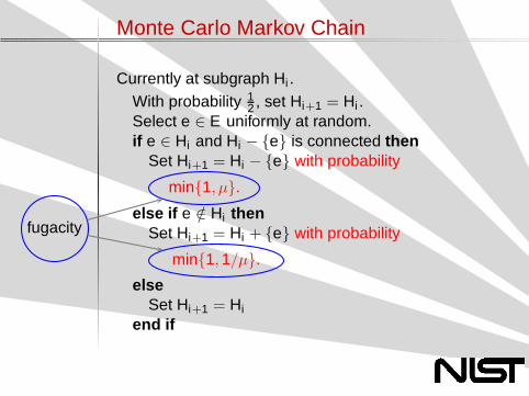
Monte Carlo Markov Chain
Currently at subgraph Hi .With probability 1
2 , set Hi+1 = Hi .Select e ∈ E uniformly at random.if e ∈ Hi and Hi − {e} is connected then
Set Hi+1 = Hi − {e} with probability
min{1, µ}.
else if e /∈ Hi thenSet Hi+1 = Hi + {e} with probability
min{1, 1/µ}.
elseSet Hi+1 = Hi
end if
fugacity
Monte Carlo Markov Chain
This yields a steady state distribution πµ where
πµ(H) =µm−|H|
Z (µ)
where
Z (µ) =
m−n+1∑
k=0
fkµk .
Problems with MCMC
◮ Mixing Time is the number of steps that must betaken before the state distribution is close enough tothe steady state.Previous Solution: If it’s not enough, take more steps.
◮ Sample size is the number of samples to take to geta good estimate of whatever is being measured.Previous Solution: Get many, many more samplesthan required.
◮ Fugacity is the value of µ used in the algorithm.Different fugacities explore different sections of thesample space.Previous Solution: Guess values, and pick more ifparts of the sample space are not explored.
Sequential Importance Sampling
Based on previous work by Beichl, Cloteaux, andSullivan.
◮ Uses Knuth’s method of estimating the size of abacktrack tree.
∑
f (X ) = E(f (X )p(X )−1).
◮ Form a tree with a subgraph at each node.
◮ Children are subgraphs with one edge removed.
◮ To estimate the number of subgraphs◮ Start with the whole graph.◮ Take out one edge at a time, without
disconnecting.◮ Note the number of choices at each step.
Example
1 2
3
5
4 6
7
a1 = 7a2 = 5a3 = 3a4 = 0
f0 = 1f1 = 7f2 = 7·5
2 = 17.5f3 = 7·5·3
3!= 17.5
Actual Values:f1 = 7f2 = 19f3 = 21
Problems with SIS
◮ Sample size How fast does the averageconverge? On many graphs, it appears toconverge very quickly, but there are pathologicalexamples where is doesn’t.
◮ People don’t use this method. (We’re trying tosolve this by telling them about it.)
Using SIS to speed up MCMC
How can we use these methods together and makeit more efficient?
◮ Run SIS first.
◮ Use the SIS results to select fugacity, calculatemixing time, and bound the sample size for usewith MCMC.
Fugacity
◮ Fugacity changes resulting steady statedistribution, indicating which area of the samplespace (which subgraphs) we are exploring.
◮ Optimal fugacity of µ = fi/fi+1 causessubgraphs of size m − i and m − i − 1 to beequally likely, all other sizes less likely.
◮ Idea: Estimate fi and fi+1 from SIS.
Calculated Fugacities
0 1 2 3 4 5 6 7 8 90
0.05
0.1
0.15
0.2
0.25
0.3
0.35
0.4
m − i (i = subgraph size)
freq
uenc
y
Expected, µ1
Expected, µ2
Expected, µ3
Expected, µ4
Expected, µ5
Expected, µ6
Expected, µ7
Expected, µ8
Expected, µ9
Actual, µ1
Actual, µ2
Actual, µ3
Actual, µ4
Actual, µ5
Actual, µ6
Actual, µ7
Actual, µ8
Actual, µ9
Fugacity chosen appropriately: Sample with fugacityµi gives a high proportion of sample subgraphs withm − i edges. (As predicted)
Aggregation
◮ The transition matrix of the Markov Chain isstochastic matrix containing the probabilities oftransitioning between each state (subgraph).
◮ There are too many states, so calculating thetransition matrix exactly is prohibitivelyexpensive.
◮ To reduce the number of states, we combinestates that are “similar” in a process calledaggregation.
◮ In this case, we are recording subgraph size, sowe combine all subgraphs of the same size intoone state.
◮ We always need many different values of the fugacity.◮ The method currently used in practice (guess and
check) does not predict the number that will beneeded.
◮ This method ensures that only the minimum number(m − n) of fugacities are needed.
◮ Mixing Time:◮ For this problem, there is no theoretical bound on the
mixing time.◮ This method calculates a mixing time on the fly for the
actual graph being measured, ensuring that theminimum number of steps are taken.
◮ Sample Size:◮ Estimation using SIS methods leads to significant
reduction in sample size from the theoretical bounds.
Extending to the Multi-variate Case
◮ In the general problem of calculating R(G; p),we let pe be the probability that an edge e isreliable. These values may be distinct fordifferent edges.
◮ There is no longer a notion of coefficients, so wemust estimate the actual value R(G; p).
◮ First algorithm uses the same search tree as inthe single variable case.
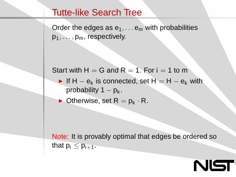
Subgraph Search Tree
For any connected H ⊆ G, letc(H) =
∏
e∈H pe∏
e/∈H(1 − pe)/(m − |H|)! and DH
the set of edges in H that are not bridges.
For any e ∈ DH , letP(e|H) = (1 − pe)/
∑
e∈CH(1 − pe).
To get the estimate, start with H0 = G, and theestimate R = c(G). For k = 1 to m − n + 1:
◮ Set Hk = Hk−1 − {e} with probability P(e|Hk−1),and set ak = P(e|Hk−1)
Compare to existing methods: Karger, basic MonteCarlo.
Compare on sparse graphs.
Tested dependence on size, density, and variance ofedge probabilities.
Size Dependence
0 10 20 30 40 5010
−5
100
105
1010
Run Number
Rel
ativ
e V
aria
nce
BMCTSSSSS
Five graphs per n, n varies from 10 to 100(increments of 10).m = 2nEarly run numbers have fewer nodes.
Size Dependence
10−10
10−5
100
10−1
100
101
102
103
104
Reliability
Rel
ativ
e V
aria
nce
BMCTSSSSS
Density Dependence
50 100 15010
0
105
1010
1015
1020
Number of eges
Est
imat
ed to
tal r
untim
e (×
ε−2 s
econ
ds)
BMCTSSSSS
Edge Variance Dependence
Trials 1–5: Uniform on (0, 1)Trials 6–10: Uniform on (0.25, 0.75)Trials 11–15: Uniform on (0, 0.25) ∪ (0.75, 1)Trials 16–20: Normal with µ = 0.5, σ = 0.25Trials 21–25: Normal with µ = 0.5, σ = 0.05Trials 26–30: Normal with µ = 0.5, σ = 0.5Trials 31–35: Uniform on (0.8, 1)Trials 36–40: Normal with µ = 0.9, σ = 0.05Trials 41–45: 1 − x , where x is exponential withλ = 0.5Trials 46–50: 1 − x , where x is exponential withλ = 0.1
Edge Variance Dependence
0 10 20 30 40 5010
−2
100
102
104
106
108
Run Number
Rel
ativ
e V
aria
nce
BMCTSSSSS
Edge Variance Dependence
0 0.05 0.1 0.15 0.210
−2
100
102
104
106
108
Variance of Edge Probabilities
Rel
ativ
e V
aria
nce
of C
alcu
late
d R
elia
bilit
y
BMCTSSSSS
Edge Variance Dependence
0 1 2 3 4 5
x 10−3
10−1
100
101
102
103
104
Variance of Edge Probabilities
Rel
ativ
e V
aria
nce
of C
alcu
late
d R
elia
bilit
y
BMCTSSSSS
Future Work
◮ Apply to larger graphs and networks, preferablyreal ones.
◮ Theoretical mixing time bound.
◮ Explore methods of reducing the sample size forlarge µ.
◮ Use SIS on other problems where we have anMCMC to increase the efficiency of the MCMCalgorithm.
◮ Theoretical results on when one multi-variatealgorithm is better than another.
◮ Apply to other Tutte polynomial calculations.
References
◮ I. Beichl, B. Cloteaux, and F. Sullivan. Anapproximation algorithm for the coefficients of thereliability polynomial. Congr. Numer., 197:143–151,2009.
◮ I. Beichl, E. Moseman, and F. Sullivan. Computingnetwork reliability coefficients. Congr. Numer.,207:111–127, 2011.
◮ D. R. Karger. A randomized fully polynomial timeapproximation scheme for the all-terminal networkreliability problem. SIAM J. Comput., 29(2):492–514(electronic), 1999.
◮ D. E. Knuth. Estimating the efficiency of backtrackprograms. Math. Comp., 29:122–136, 1975. Collectionof articles dedicated to Derrick Henry Lehmer on theoccasion of his seventieth birthday.