52
Network Simplex Method Fatme Elmoukaddem Jignesh Patel Martin Porcelli
| Date post: | 01-Jan-2016 |
| Category: |
Documents |
| Upload: | brenden-tanner |
| View: | 75 times |
| Download: | 6 times |

Network Simplex Method
Fatme Elmoukaddem
Jignesh Patel
Martin Porcelli

Outline
• Definitions
• Economic Interpretation
• Algebraic Explanation
• Initialization
• Termination

Transshipment Problem
• Find the cheapest way to ship prescribed amounts of a commodity from specified origins to specified destinations through a transportation network
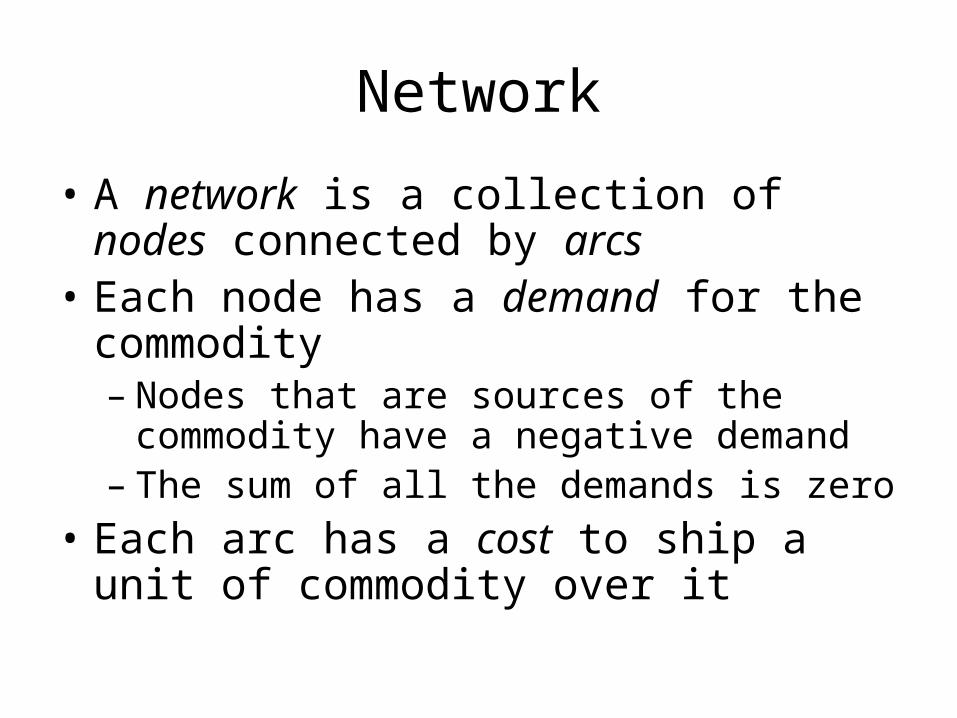
Network
• A network is a collection of nodes connected by arcs
• Each node has a demand for the commodity– Nodes that are sources of the commodity
have a negative demand– The sum of all the demands is zero
• Each arc has a cost to ship a unit of commodity over it

Example
1
2
3
4
5
-5
1
3
3
-2
5
4
7
3
9
1
5

Schedule
• A schedule describes how much of the commodity is shipped over each arc
• Requirements– The amount entering a node minus the
amount leaving it is equal to its demand– The amount shipped over any arc is
nonnegative

Example
1
2
3
4
5
-5
1
3
3
-2
1
3
1
0
0
0
2

LP Formulation
• Let c be a row vector and x a column vector indexed by the set of arcs– cij is the cost of shipping over ij
– xij is the amount to ship over ij
• Let b be a column vector indexed by the set of nodes– bi is the demand at i

Example
1
2
3
4
5
-5
1
3
3
-2
5
4
7
3
9
1
5
5193745c
54
35
25
23
14
13
12
x
x
x
x
x
x
x
x
23315 b

LP Formulation
0
0
ii
iij
ijji
ji
ij
ijijij
b
bxxi
xij
xc to subject minimize cx
LP Formulation (2)
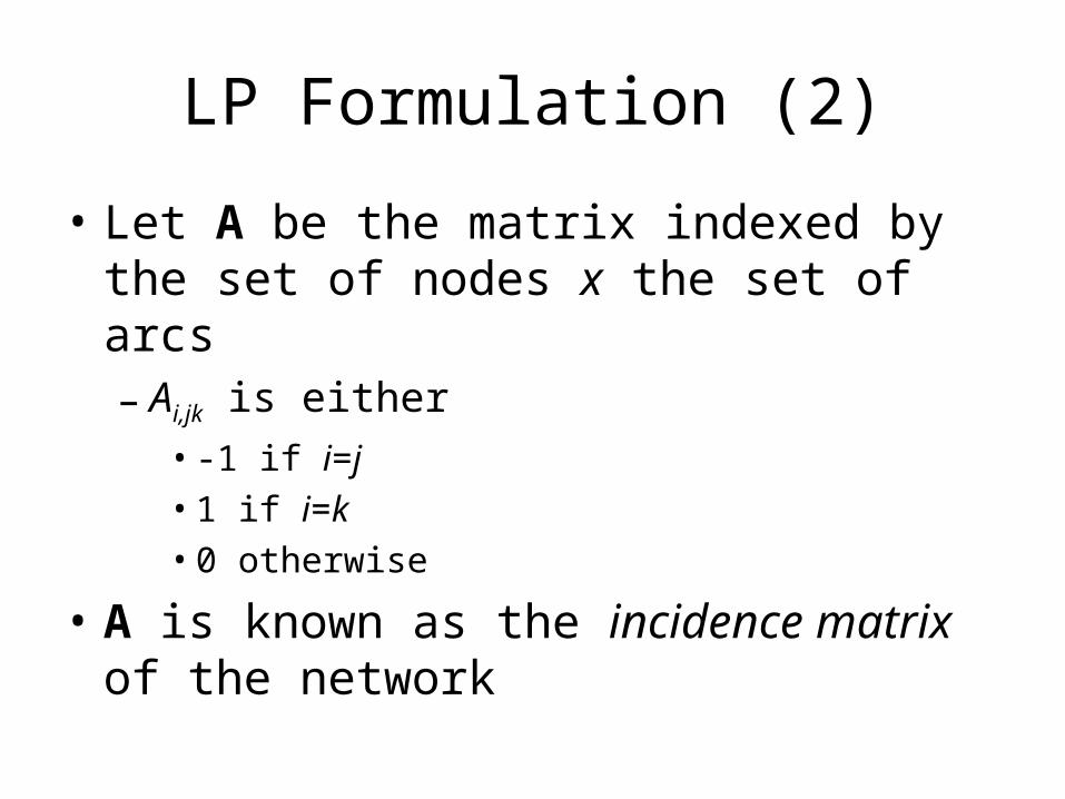
• Let A be the matrix indexed by the set of nodes x the set of arcs– Ai,jk is either
• -1 if i=j• 1 if i=k• 0 otherwise
• A is known as the incidence matrix of the network

Example
1
2
3
4
5
-5
1
3
3
-2
5
4
7
3
9
1
5
1110000
1000100
0101010
0011001
0000111
5
4
3
2
154352523141312

LP Formulation (2)
0
0
i
i
ij
b
xij
bAx
cx to subject minimize

Tree Solution
• A spanning tree of a network is a network containing every node and enough arcs such that the undirected graph it induces is a tree
• A feasible tree solution x associated with a spanning tree T is a feasible solution with– xij = 0 if ij is not an arc of T

Network Simplex Method
• Search through feasible tree solutions to find the optimal solution
• Has a nice economic interpretation

Economic Interpretation
• Given a spanning tree T and an associated feasible tree solution x
• Imagine you are the only company that produces the commodity
• What price should you sell the commodity for at each node?– Assume that you ship according to x
Price Setting
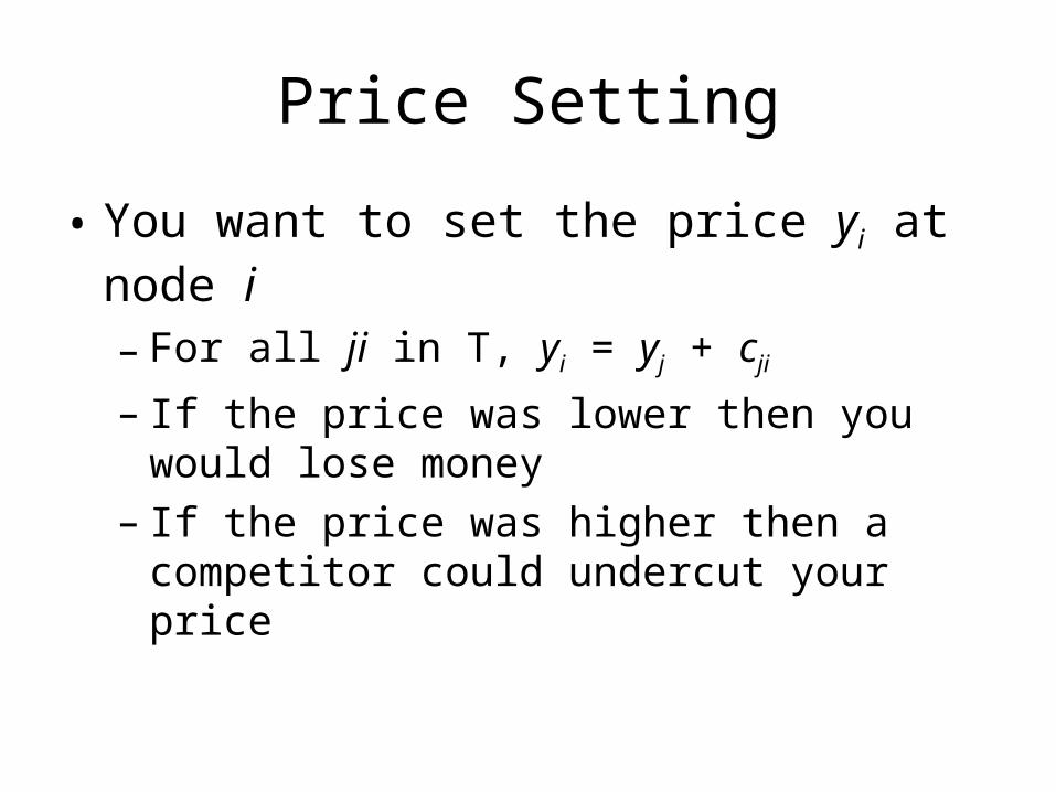
• You want to set the price yi at node i
– For all ji in T, yi = yj + cji
– If the price was lower then you would lose money
– If the price was higher then a competitor could undercut your price

Problem / Solution
• A competitor could still undercut your price – If there was an arc ki not in T with yi > yk + cki
• You don’t want to lose business, so you also plan to ship over ki– You want to ship as much as possible– You must also adjust the rest of your
schedule to conform with demand
Example
1
2
3
4
5
0
5
8
7
2
5
7
3
5
4
1
2
3
4
5
0
5
4
7
2
5
4
7
5

Optimality
• If no arc like ki exists, then your prices can not be undercut– A competitor could break even at best

Algebraic Description (Step 1)
• Each step begins with a feasible tree solution x defined by a tree T.– x is a column vector with a flow value for each arc.
• In step 1 we calculate a value for each node such that yi + cij = yj, ij T.– y is a row vector with value of each node.
• c is the cost (row) vector, b is the demand (column) vector, and A is the incidence matrix.

Algebraic Description (Step 1)
1
2
4
3
2
3
0
2
0
-5 3
20
T:
1
2
4
3
1
7
3
9
5
-5 3
20
G:
5 3 9 7 1
3
2
0
5
0
0
2
3
2
11010
10100
01101
00011
4
3
2
13424231412
71010
c
y
bxA

Algebraic Description (Step 1)
• We define c’ = c – yA.• c’ is the difference between the cost of an arc
and the value difference across the arc.
• If ij T then c’ij = cij + yi – yj = 0.
• If ij T and if c’ij < 0 then ij is candidate for entering arc.
• Also if ij T then xij = 0, combining with above we get c’x = 0 ( ij, either c’ij = 0 or xij=0).

Algebraic Description (Step 1)
1
2
4
3
2
3
0
2
0
-5 3
20
T:
1
2
4
3
1
7
3
9
5
-5 3
20
G:
8 3-0 0 0 '53971
3
2
0
5
0
0
2
3
2
11010
10100
01101
00011
4
3
2
13424231412
71010
c
c
y
bxA

Algebraic Description (Step 1)
• For any feasible solution x’ (i.e. Ax’ = b,x’ ≥ 0), its cost is
cx’ = (c’ + yA)x’ (c’ = c - yA)= c’x’ + yAx’= c’x’ + yb. (Ax’ = b)
• In particular for x, its cost is cx = c’x + yb = yb. (c’x = 0)
• Substituting for yb in the cost of x’ we get cx’ = cx + c’x’ (1)
• So if c’x’ < 0 then x’ is a better solution than x.

Algebraic Description (Step 2)
• In step 2 we find an arc e = uv such that yu + cuv < yv (i.e. c’uv < 0).
• If no such arc exists then c’ ≥ 0 and so c’x’ ≥ 0.
• Hence equation (1) implies cx’ ≥ cx for every feasible solution x’, and so x’ is optimal.
• If we find such an arc e, we it to the tree T.

Algebraic Description (Step 3)
• For step 3, T + e has a unique cycle.
• Traversing the cycle in the direction of e we define forward arcs as arcs pointing in the same direction as e and reverse arcs as arcs pointing in the opposite direction.
• Then we set
cycle. on thenot is if
arc, reverse a is if
arc, forward a is if
ijx
ijtx
ijtx
x
ij
ij
ij
ij

Algebraic Description (Step 3)
1
2
4
3
2+t
3-t
t
2
0
-5 3
20
T+e:
0
0
2
3
2
0
0
2
3
2'
83000
'
t
t
txx
c
1
2
4
3
2
3
0
2
0
-5 3
20
T:

Algebraic Description (Step 3)
• Now, Ax’ = Ax = b, because for each node of the cycle the extra ±t cancel each other.
• So if we choose t such that x’ ≥ 0, then x’ is feasible.
• Since e is the only arc with c’ij 0 and x’ij 0, we have c’x’ = c’ex’e = c’et.
• Substituting in equation (1) we get cx’ = cx + c’et.
• We want to choose t such that x’ is feasible and which minimizes cx’.

Algebraic Description (Step 3)
• We have, cx’ = cx + c’et.
• Since c’e < 0, to minimize cx’, we have to maximize t.
• To make sure x’ is feasible (i.e. x’ ≥ 0), we find a reverse arc f with minimal value xf, and let t = xf.
• The new feasible solution x’ has x’f = 0, so f is the leaving arc.
• Removing f breaks the only cycle in T + e, so T + e – f is the new tree that defines the new feasible tree solution x’.

Degeneracy and Cycling
• If there is more than one candidate for the leaving arc, then for each candidate arc ij,x’ij = 0.
• Only one of the candidate arcs leaves the tree, so the new solution has x’ij=0 for at least one of its tree arcs.
• Such a solution is called a degenerate solution.• They could lead to pivots with t = xf = 0, that is
no decrease in the cost.• Degeneracy is necessary but not sufficient for
cycling.

Degeneracy and Cycling
1
2
4
3
3-t
3-t
t
2
0
0 3
2-5
T+e:
1
2
4
3
3
3
0
2
0
0 3
2-5
T:
1
2
4
3
1
7
3
9
5
0 3
2-5
G:
1
2
4
3
0
0
3
2
0
0 3
2-5
T+e-f:

Degeneracy and Cycling
• Cycling is very rare. No practical example with cycling has been found.
• The first artificial example was constructed 13 years after the appearance of the network simplex method.
• Cycling can be avoided by proper choice of the leaving arc. We will see this later.

Initialization
• If there is a node w | there is an arc:– from every supply node to w– from w to every sink/intermediary node
Then there is an initial feasible solution
wsupply sinks
intermediary

Initialization
• If no such w, add artificial arcs
• Associate a penalty pij for using these arcs ij:– pij = 0 for original arcs
– pij = 1 for artificial arcs
• Solve auxiliary problem: Min pijxij

Initialization
i. T contains an artificial arc ij with xij > 0
=> Original problem has no feasible sol
ii.T contains no artificial arc=> T is a feasible sol. for original problem
iii. Every artificial arcs ij in T has xij = 0
=> original problem has a feasible sol. But not a feasible tree sol.

Decomposition
• For each set S and feasible solution x:
– Import – Export = Net demand– In Ax = b, sum equations corresponding to
nodes in S
Sk
k
SjSi
ij
SjSi
ij bxx
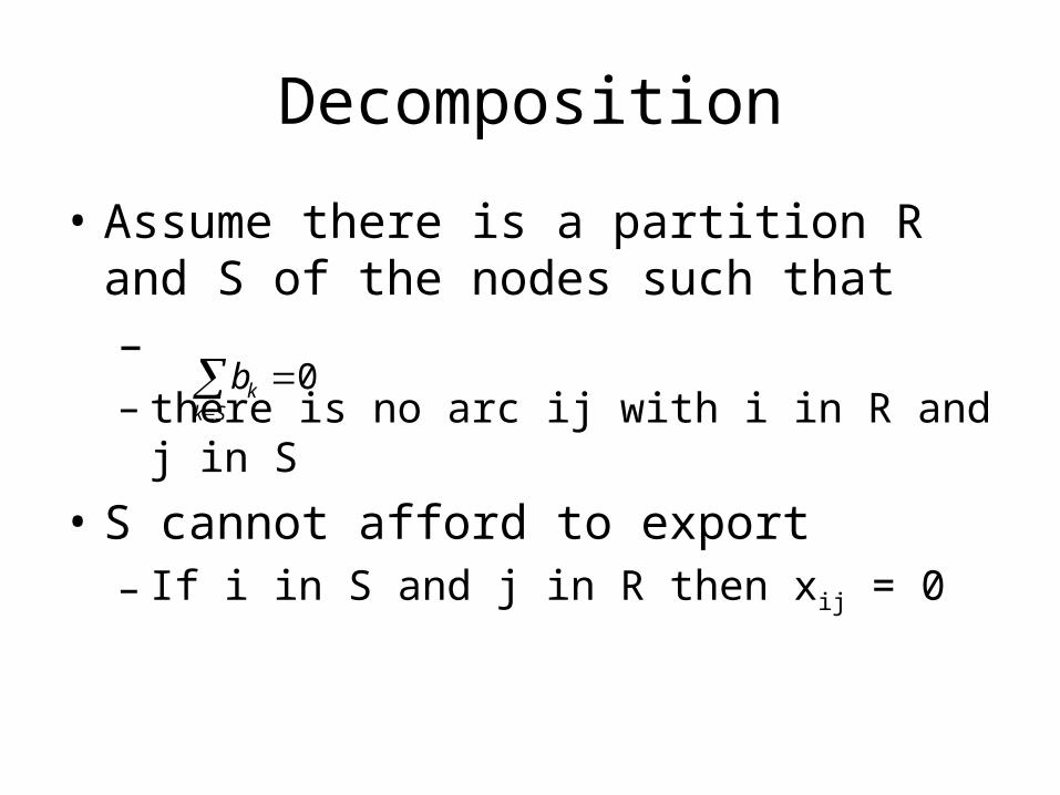
• Assume there is a partition R and S of the nodes such that– – there is no arc ij with i in R and j in S
• S cannot afford to export– If i in S and j in R then xij = 0
Decomposition
Sk
kb 0

Decomposition
-5
2
-2
2
3
-3
3
-5
2
-2
2
3
-3
3
S R

Decomposition
Decompose optimal tree T of auxiliary problem same way:
Take arbitrary artificial arc uv
k in R if yk yu and k in S otherwise
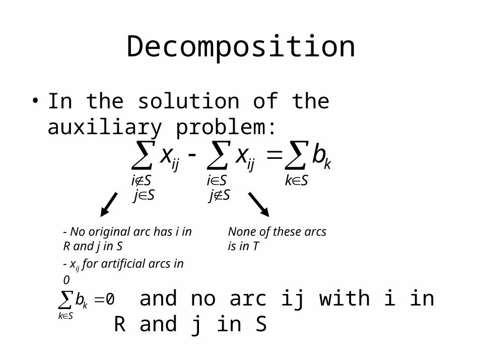
Decomposition
• In the solution of the auxiliary problem:
Sk
k
SjSi
ij
SjSi
ij bxx
None of these arcs is in T
- No original arc has i in R and j in S
- xij for artificial arcs in 0
and no arc ij with i in R and j in S
Sk
kb 0

Updating nodes
In T: yi + cij = yj, ij in T
Goal: y’i + cij = y’j, ij in T + e – f
Define:
y’k = yk (k in Tu)
yk + c’e (k in Tv)
c’e = ce + yu – yv
e
f
uv

Avoid Cycling
Direction of an arc with respect to root
wt
a

Avoid Cycling
Thm: If each degenerate pivot leads from T to T + e – f such that e is directed away from the root of T + e – f => no cycling
Avoid Cycling
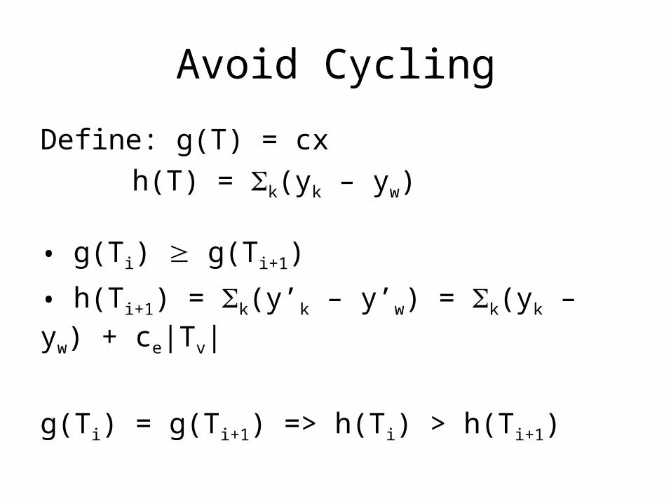
Define: g(T) = cx
h(T) = k(yk – yw)
• g(Ti) g(Ti+1)
• h(Ti+1) = k(y’k – y’w) = k(yk – yw) + ce|Tv|
g(Ti) = g(Ti+1) => h(Ti) > h(Ti+1)

Avoid Cycling
Ti = Tj, i < j =>
g(Ti) = g(Ti+1) = … = g(Tj)
h(Ti) > h(Ti+1) > … > h(Tj)
Contradicting h(Ti) = h(Tj)

Avoid Cycling
Strongly feasible: all arcs ij in T | xij = 0 are directed away from the root
1. initial solution is strongly feasible
2. if T is strongly feasible, then T + e – f is strongly feasible
=> No cycling

Avoid Cycling
1. Starting with a strongly feasible:
Bad arc: directed toward the root and xarc = 0
i. Start with T
ii. Remove bad arc uv: Tv and Tu
iii. If there is an arc ij | i in Tv and j in Tu, add ij to T
=> T’ with less bad arcs
else decompose into two subproblems

Avoid Cycling
2. Arrive at a strongly feasible solution:
Entering arc: any candidate
Leaving arc: first candidate while traversing C in direction of e starting at the join
wjoin
entering arc

Avoid Cycling
Case 1: the pivot is non-degenerate
join
candidate
candidatecandidate
entering
candidate
Candidate arcs ij:
• will have xij = 0 in the new sol.
• will be directed away from w

zero
zero
zero
candidate
candidate
candidate
Avoid Cycling
Case 2: the pivot is degenerate
join
No reverse zero arcs
No forward zero arcs
zero
zero
candidate
zero

Questions?


