Network State Classification Based on the Statistical Properties of RTT for an Adaptive Multi-State...

8/8/2019 Network State Classification Based on the Statistical Properties of RTT for an Adaptive Multi-State Proactive Transpo…

http://slidepdf.com/reader/full/network-state-classification-based-on-the-statistical-properties-of-rtt-for 1/20

International Journal of Computer Networks & Communications (IJCNC) Vol.2, No.6, November 2010

DOI : 10.5121/ijcnc.2010.2611 155

NETWORK S TATE CLASSIFICATION BASED ON THE

S TATISTICAL PROPERTIES OF RTT FOR AN

A DAPTIVE MULTI-S TATE PROACTIVE TRANSPORT

PROTOCOL FOR S ATELLITE BASED NETWORKS

Mohanchur Sakar 1, K.K.Shukla 2 and K.S.Dasgupta2

1Space Applications Centre (ISRO), Ahmedabad, Gujarat, [email protected]|[email protected],[email protected]

2Department of Computer Engineering, I.T, BHU, Varanasi, U.P, [email protected]

A BSTRACT

This paper attempts to establish the fact that Multi State Network Classification is essential for performance enhancement of Transport protocols over Satellite based Networks. A model to classify

Multi State network condition taking into consideration both congestion and channel error is evolved. In

order to arrive at such a model an analysis of the impact of congestion and channel error on RTT values

has been carried out using ns2. The analysis results are also reported in the paper. The inference drawn

from this analysis is used to develop a novel statistical RTT based model for multi state network

classification. An Adaptive Multi State Proactive Transport Protocol consisting of Proactive Slow Start,

State based Error Recovery, Timeout Action and Proactive Reduction is proposed which uses the multi

state network state classification model. This paper also confirms through detail simulation and analysis

that a prior knowledge about the overall characteristics of the network helps in enhancing the

performance of the protocol over satellite channel which is significantly affected due to channel noise and

congestion. The necessary augmentation of ns2 simulator is done for simulating the multi state network

classification logic. This simulation has been used in detail evaluation of the protocol under varied levels

of congestion and channel noise. The performance enhancement of this protocol with reference to

established protocols namely TCP SACK and Vegas has been discussed. The results as discussed in this paper clearly reveal that the proposed protocol always outperforms its peers and show a significant

improvement in very high error conditions as envisaged in the design of the protocol. The protocol is also

evaluated to have very good fairness property under different error conditions.

K EYWORDS

GEO, ns2, Proactive TCP, SACK, Vegas, Adaptive

1. INTRODUCTION

TCP has become the de-facto protocol standard for congestion control in the existing terrestrialInternet. However, experimental and analytical studies [13] confirm that the current TCPprotocol variants have performance problems in long fat networks coupled with very highwireless channel errors like satellite networks [16], [15], [21]. Satellite based Networks aredominated by random packet errors which are not common in the wired counterpart. TCPprotocols react to the lack of arrival of acknowledgments or duplicate ACK as a sign of congestion. So the congestion window is reduced which leads to unnecessary throughputdegradation [13]. It is a challenge for the network researchers and protocol developers to findmeans to differentiate the cause of the DUP ACK arrival. Generally probing is done in protocolslike Peach [1], Peach+ [2], TP-Planet [3] and RCS [4] but at the cost of bandwidth used for thelow priority dummy packets.




156

Majority of the Transport Protocols tries to ascertain the condition of the network in terms of anestimation of the prevailing congestion in the network [8]. This is because of the fact that thebasic paradigm on which the conventional TCP protocols evolved was based on a wiredconnectivity where congestion was the primary concern. The channel noise was not taken intoaccount mainly due to the fact that wired connectivity can be through of as an errorless channel

[13]. So the network states were broadly classified into two states congested and uncongested.But when TCP Protocols are used for Satellite based Networks the effect of wireless channelerrors also become significant [16]. Hence this assumption of two state concept does not lead tothe most optimal performance. It is obvious from the above mentioned reasons that use of TCPover Satellite channel need to address equally the effect of congestion and channel noise whichare important detrimental factors for performance degradation [13][21]. To handle the problemsquarely one need to consider Multi State representation of network condition. There is a needto develop a model to handle and represent Multi State network conditions for satellite basedTCP/IP networks. In order to formulate the model and understand the various systemparameters which control it, the model need to be explicitly evolved and analyzed.

The inferences from this analysis as discussed in this paper are used in an innovative way towork out an Adaptive Multi-State Proactive Transport Protocol with a view to improve theoverall network performance over a Satellite channel which has high degree of channel noiseand appreciable congestion. In order to formulate the Multi-State Network classification modeldetail simulation based experiments in ns2 [12] have been carried out to ascertain the combinedeffect of congestion and channel error on the RTT values pertaining to a connection. Theinference from these simulation experiments has been used in the evolution of a Statisticalmodel for network state classification based on RTT values.

The paper is organized as follows. We introduce the RTT Analysis for Multi State Model inSection 2. In Section 3, we propose the statistical formulation of model parameters. Section 4describes the hierarchical network state classification method. Section 5 describes the AdaptiveMulti State Proactive Transport protocol. Section 6 describes the design considerations of theproposed protocol. Section 7 details the Test and Evaluation methodology. Finally, in Section 8we conclude the paper.

2. RTT ANALYSIS FOR MULTI STATE MODEL

The primary goal of the model is to carry out multi state classification of network states with aview to differentiate (i) No Congestion No Error, (ii) No Congestion High Error, (iii) HighCongestion No Error and (iv) High Congestion High Error conditions of the network. This willbe a significant departure from the conventional two state network classification model withstates (i) No Congestion and (ii) Congestion. Using the four states model the combined effect of congestion and corruption on the network can be ascertained. This model will be primarilyworked out to handle the performance degradation of TCP over satellite channel where there iscoexistence of channel noise and congestion. For the formulation of the model simulation basedexperiments have been carried out in ns2 [12] to study and analyze the impact of congestion andchannel errors on the model parameters. The inference of these analysis will help us inunderstanding a set of network system parameters which can be properly incorporated in the

proposed Adaptive Multi State Proactive Transport Protocol.

2.1. RTT based Modelling Philosophy

When a TCP connection is in progress, the sender has no idea about what is happening in thenetwork. It only receives the ACKS, sometimes duplicate ACKS and encounters timeout whenthe ACKs do not come within an anticipated time[22]. From the received ACKs, the RTT is the




157

only information available to the sender which can be used for a proactive decision makingregarding the state of the network.

2.2. Use of RTT Mean

The RTT in general is considered to be an independent random variable [9]. While a TCP

connection proceeds, if we measure the individual RTT values for every window for all thesegments transmitted in that window, it will not convey much information regarding thecondition of the network, as the transient RTT values are dependent on many dynamic networkparameters which changes so frequently that no stable conclusion can be drawn from them.Moreover as suggested in [19], the frequency with which we sample the RTT values isgenerally less than the Nyquist’s Sampling frequency requirement if we consider the RTTvalues as a time varying signal. So as the sampling is done at a rate lower than needed a properreconstruction of the signal will not be possible and there is a chance to respond to valuescorrupted with noise. Another important point is that in a network there are many connectionssharing a common bandwidth, so an increase or decrease in RTT cannot be attributed to behappening because of that particular connection and taking action on the individual RTT valuesmay not generate optimal conclusion [19][23]. So we have considered the mean of all the RTTvalues in a window, which convey more information or may be thought of as a more

representative value of the RTT for that specific window to be used in our RTT based model.

2.3. Simulation based Experimental Results

In this paper, we have performed some simulation based experiments using ns2[12] with thesimulation setup of 10 senders transmitting to 10 receivers over a GEO link as described inSection 7, to find out the impact of network congestion and packet error rates on the RTTvalues. These simulation based experiments are needed in the formulation of the Multi Staterepresentation of network condition. Three classes of experiments have been performed, (i)considering an uncongested network, (ii) considering a congested network and (iii) progressivelevels of network congestion but with very less channel errors

2.4. Analysis of Results

In Fig.1 to Fig. 9 the mean RTT values are plotted with simulation time for a TCP connection asthe simulation progresses. First, we have considered the packet error rate to be 0 and it can beseen from Fig. 1 that the mean RTT remains in a closed range of 560 to 570 ms. On the contraryin Fig. 5 even with PER 0, the mean RTT values are more dispersed which shows the effect of congestion on the RTT values. In both the network conditions we have gradually increased thepacket error rate from PER 0.001 to PER 0.1 and it has been observed that as we increase thePER for uncongested network the values are seen to have more frequent flickers and dispersionincreases. In a congested network condition the effect is more pronounced than its uncongestedcounterpart for the same PER value. It has also been observed that congested network conditionleads to an increase in the DC value of the concerned parameter, larger dispersion and flickeringof mean RTT. In Fig. 9 to ascertain the effect of congestion on mean RTT values we haveintentionally infused higher levels of congestion in the network, by chocking the availablebandwidth to the satellite to lower values of 4Mbps, 3Mbps down to 1Mbps where the optimum

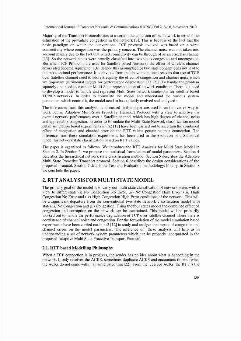
bandwidth required is 5 Mbps as described in Section 7 in detail. Fig.9 directly depicts the highcorrelation, the DC value of the RTT mean has with increasing levels of congestion. Thesimulation experiment used a GEO satellite link having RTT around 550 to 570 ms. In thesimulation scenario decreasing bottleneck bandwidth between the two earth stations theindividual maximum bandwidth shared by the connections can be though of as reducing from500 kbps to 100 kbps. The mean RTT values are seen to increase and to be hovering in therange of 570 ms, 700ms, 900ms, 1400ms and 2700ms corresponding to the decrease in linkcapacity and increasing degree of congestion [22][24]. The inferences which can be drawn from




158

these experiments are given below as (i) From the first experiments it can be concluded that nocongestion and no error leads to very less dispersion of the mean RTT values, dispersionincreases with increasing PER (ii) From second experiment it can be concluded that under

550

555

560

565

570

575

0 100 200 300 400 500 600

Simulation Time (s ecs)

M e a n R T T ( m s )

550

560

570

580

590

600

610

620

630

0 100 200 300 400 500 600

Simulation Time (se cs)

M e a n R T T ( m s e c s )

Fig. 1 PER = 0.00 Queue = 20 Max Receiver Win = 20 Fig. 5 PER = 0.00 Queue = 64 Max Receiver Win = 64

550

560570

580

590

600

0 200 400 600

Simulation Time (secs)

M e a n R

T T ( m s e c s )

550

570

590

610

630

650

670

690

710

730

750

0 100 200 300 400 500 600

Simulation Time (s ecs)


Fig. 2 PER = 0.001 Queue=20 Max Receiver Win= 20 Fig. 6 PER = 0.001 Queue = 64 Max Receiver Win= 64

550

560

570

580

590

600

610

620

630

0 100 200 300 400 500 600

Simulation Time (secs )


550

750

950

1150

1350

1550

0 100 200 300 400 500 600



Fig. 3 PER = 0.01 Queue = 20 Max Receiver Win= 20 Fig. 7 PER = 0.01 Queue = 64 Max Receiver Win = 64

550

650

750

850

950

1050

1150

1250

0 100 200 300 400 500 600



550

650

750

850

950

1050

1150

1250

0 100 200 300 400 500 600



Fig. 4 PER = 0.1 Queue = 20 Max Receiver Win = 20 Fig. 8 PER = 0.1 Queue = 64 Max Receiver Win = 64




159

500

1000

1500

2000

2500

3000

0 100 200 300 400 500 600



B = 500 k bps B = 400 k bps B = 300 k bps

B = 200 kbps B = 100 kbps

Fig. 9 RTT Mean Variation For Different Congestion Levels

congested condition, the increase in packet error rate leads to more dispersion of mean RTTvalues. (iii) From the third experiment it can be concluded that if channel error is very less thedegree of congestion is directly related to the increase in DC value of the RTT Mean. So it canbe concluded that RTT has multivariate correlation [23] with congestion and PER prevailing inthe network.

3. STATISTICAL FORMULATION OF MODEL PARAMETERS

In this section, considering this inference discussed in Section2 we have developed a model to

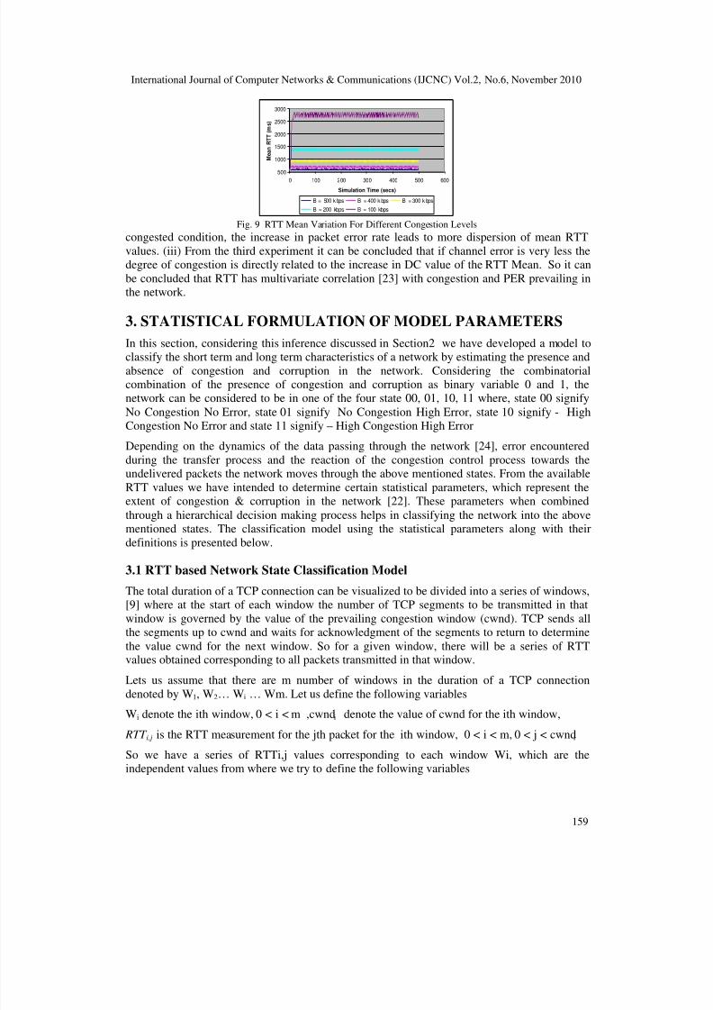
classify the short term and long term characteristics of a network by estimating the presence andabsence of congestion and corruption in the network. Considering the combinatorialcombination of the presence of congestion and corruption as binary variable 0 and 1, thenetwork can be considered to be in one of the four state 00, 01, 10, 11 where, state 00 signifyNo Congestion No Error, state 01 signify No Congestion High Error, state 10 signify - HighCongestion No Error and state 11 signify – High Congestion High Error

Depending on the dynamics of the data passing through the network [24], error encounteredduring the transfer process and the reaction of the congestion control process towards theundelivered packets the network moves through the above mentioned states. From the availableRTT values we have intended to determine certain statistical parameters, which represent theextent of congestion & corruption in the network [22]. These parameters when combinedthrough a hierarchical decision making process helps in classifying the network into the above

mentioned states. The classification model using the statistical parameters along with theirdefinitions is presented below.

3.1 RTT based Network State Classification Model

The total duration of a TCP connection can be visualized to be divided into a series of windows,[9] where at the start of each window the number of TCP segments to be transmitted in thatwindow is governed by the value of the prevailing congestion window (cwnd). TCP sends allthe segments up to cwnd and waits for acknowledgment of the segments to return to determinethe value cwnd for the next window. So for a given window, there will be a series of RTTvalues obtained corresponding to all packets transmitted in that window.

Lets us assume that there are m number of windows in the duration of a TCP connectiondenoted by W1, W2… Wi … Wm. Let us define the following variables

Wi denote the ith window, 0 < i < m ,cwndi denote the value of cwnd for the ith window,

RTT i,j is the RTT measurement for the jth packet for the ith window, 0 < i < m, 0 < j < cwndi

So we have a series of RTTi,j values corresponding to each window Wi, which are theindependent values from where we try to define the following variables




160

i

cwnd

j

ji

icwnd

RTT

MW

i

∑=

=0

,

(1)MWi denote the mean of the RTT values for the ith window Wi

k

MW

M

i

k i j

j

k

∑−=

= (2)

Mk denotes the window average of the mean values MW j for the last k windows.

IRTT

IRTT M MR k

k

−

= (3)

MRk denote the normalized rise of the mean RTT values from the ideal RTT values. IRTT canbe determined from previous knowledge of the end to end delay and is given by the minimum of all RTT values measured for that specific connection. So IRTT in the beginning will be equal tothe RTT values obtained through the SYNC message exchanged during connection setup andgradually can be refined with new values. MRk is an estimation of the short term condition of the network load. MWi denote the mean of the RTT values for the ith window Wi.

i

MW

M

i

j

j

i

∑=

=

0(4)

In (2) if we replace k with i then we get the long term mean M i which is equal to the mean of allthe mean values MW j obtained for each window from the beginning. So the Mk values give theshort term characteristics of the network and M i gives the long term characteristics as it is theintegration of all the values the connection has experienced from its inception. Similarly MR i

denotes the long term mean rise as given below where i denote the prevailing window. So as theconnection progresses, at each instant if the prevailing window is i, then MRi denotes the rise of the mean from the ideal value considering values from beginning of connection.

IRTT

IRTT Mi

MRi

−

=

(5)

Next we calculate the standard deviation of the mean rtt values, MW j for the last k windows,

k

M MW i

k i j

k j

k

∑−=

−

=

2)(

σ (6)

Here k denotes the number of last window values considered.

i

M MW i

j

i j

i

∑=

−

=

0

2)(

σ (7)

IRTT R k

k

σ = (8)

Rk denotes the ratio of the standard deviation to the ideal RTT which signifies the extent towhich the RTT values have been dispersed from the ideal condition. Ri is the long term ratio.

IRTT R i

i

σ = (9)

The parameter Sk denotes the ratio in which the intermediate Mean RTT values MW j and MW j+1




161

have not changed beyond a threshold α to the total number of windows considered. In our case α is taken as 1% of previous RTT Mean so, α = 0.01 * MWj. Sk denotes the short term stability of the network.When k is replaced by i, Si denotes the stability of the connection from the beginning. In theRTT based Model for network state classification we have defined some statistical parametersfrom the measured rtt values which convey different meaning about the short term and longterm characteristics of the network. So corresponding to each window Wi we can think of theset of values {MR10, MR20, MR30, MRi}for Mean Rise, the set {R10, R20, R30, Ri} for Ratio andfor stability {S10,S20, S30, Si} to signify the short term and long term characteristics of thenetwork. The way these parameters varies under different network state is shown below.

0

0.5

1

1.5

2

2.5

3

3.5

4

4.5

0 100 200 300 400 500 600simulation time (secs)

M R 1 0

State00 State01 State10 State11

0

0.5

1

1.5

2

2.5

3

3.5

4

4.5


M R 2 0


Fig. 10 Mean Rise Window Average Length = 10 Fig. 13 Mean Rise Window Average Length = 20

0

0.2

0.4

0.6

0.8

1

1.2

1.4

1.6

1.8

0 100 200 300 400 500 600

Simulation Time(secs)

R 1 0


0

0.5

1

1.5

2

0 100 200 300 400 500 600


R 2 0


Fig. 11 Ratio Window Average Length = 10 Fig. 14 Ratio Window Average Length = 20

-0.2

0

0.2

0.4

0.6

0.8

1

1.2

0 100 200 300 400 500 600


S 1 0


0

0.2

0.4

0.6

0.8

1

1.2

0 100 200 300 400 500 600


S 2 0


Fig. 12 Stability Window Average Length = 10 Fig. 15 Stability Window Average Length = 20

3.2 Short Term Network Characteristics

The short term characteristics of the network can be obtained by considering a window average

of some fixed number of past windows. This will give us a more recent condition of thenetwork. We have simulated considering the last 10, 20 and 30 windows which are displayed inthe graph below. All the three parameters considered in the protocol like mean rise, ratio andstability is seen to vary as shown in Fig. 10 to Fig. 18.




162

3.3 Long Term Network Characteristics

From the Fig. 10 to Fig. 21 it can be seen that as the value of the parameter k increase from 10to 20 to 30, the standard deviation of all the individual plotted statistical parameters is seen toreduce. This is obvious considering the principle of the sampling theory, that a larger samplereduces the standard deviation of the sample mean and leads to a more accurate estimation of the population concerned. So, the long term estimate MRi, Ri and Si is seen to have much less

dispersion in Fig. 19, Fig. 20 and Fig. 21 as the simulation time progresses, therebycharacterizing the network into its different states. So the variable MRi, Ri and Si canbe considered as the network state variables and for each progressive window, getupdated as per the equations described above.

0

0.5

1

1.5

2

2.5

3

3.5

4

4.5


M R 3 0


0

0.5

1

1.5

2

2.5

3

3.5

4

4.5


M R i


Fig. 16 Mean Rise Window Average Length = 30 Fig. 19 Mean Rise Window Average Length = i

0

0.5

1

1.5

2

0 100 200 300 400 500 600


R 3 0


0

0.2

0.4

0.6

0.8

1

1.2

1.4

1.6

1.8

0 100 200 300 400 500 600


R i


Fig. 17 Ratio Window Average Length = 30 Fig. 20 Ratio Window Average Length = i

-0.2

0

0.2

0.4

0.6

0.8

1

1.2

0 100 200 300 400 500 600


S 3 0


0

0.1

0.2

0.3

0.4

0.5

0.6

0.7

0.8

0.9

0 100 200 300 400 500 600


S i

S ta te 00 S tat e0 1 S ta te 10 S tat e1 1 Fig. 18 Stability Window Average Length = 30 Fig. 21 Stability Window Average Length = i

4. HIERARCHIAL NETWORK STATE CLASSIFICATION

This section describes the network state classification logic along with the classification of thestatistical parameters described in Section3. The equations to derive the thresholds have beenexplained considering values derived from simulation experiments. Table I, Table II and TableIII contain values of parameter MRi, Ri and Si respectively calculated from simulations,considering the scenario described in Section 7 for a Geo Satellite Network. In Section 5 it willbe shown how the Parameter Adaptation Algorithm automatically generates the Tablesdescribed in this section. A pictorial representation of the parameter classification logic alongwith multi state hierarchical network classification logic is also presented in this section.




163

4.1Mean Rise Classification

Table I gives the minimum and maximum value obtained by the Mean Rise, MRiparameter through the simulation experiment under different network states.

TABLE1MEAN RISE VALUES FOR GEO NETWORK (MRi)

State 00 01 10 11Min 0.031 0.1 0.40 0.20Max 0.10 0.2 3.96 0.50

Let us define the following thresholds LMRi and HMRi which differentiate the MRi value intolow (L), medium (M) and high (H) ranges as shown in Fig. 22

{ }01,00 State MRState MR Max LMRiii

= (10) { }11State MR Max HMRii

= (11)

LMRi denotes the lower threshold is given by the max value obtained by MRi in 00 and 01states. So when the value of MRi is below this threshold we can assume that the network is in00 or 01 state. HMRi denotes the upper threshold is given by the max value obtained by MRi instate 11. When the value of MRi is between LMRi and HMRi the network is estimated to beeither in state 10 or 11. MRi values higher than HMRi denotes the high congestion no error stateof 10. Fig. 22 shows the classification of network states using MRi.

4.2. Ratio based Classification

The following table gives the minimum and maximum value obtained by the Ratio parameter Rithrough the simulation experiment. We define a threshold

{ }00State R Max LRii = (12)

TABLE IIRATIO VALUES FOR GEO NETWORK (Ri)

00 01 10 11Min 0.013 0.23 0.179 0.35Max 0.2 0.3 1.2 0.40

LRi is used as a threshold which divides the ratio values into two broad cases low (L) and high

(H) and any value lower than the threshold can be considered to be a sign that the network is instate 00. If values higher than this are obtained then the network can be in either of the states 01,10 and 11 as shown below.

Fig. 22 Classification of Network states using Mean Rise MRi Fig. 23 Classification of Network states using Ratio Ri

4.3. Stability based ClassificationThe following table shows the values of the stability parameter obtained through simulationexperiment. We can define some threshold, which differentiate the stability parameter into Low(L), Medium (M) and High (H) values classifying the network into states as shown in the Fig.24. Let us define the thresholds

{ }10StateS Max LSii

= (13) { }01,00 StateSStateS Min HSiii

= (14)

Mean Rise (MRi)

L00 , 01

M10, 11 H

10

<= 0.2

0.2 - 0.5

> 0.5

Ratio (Ri)

L00

H01, 10, 11

<= 0.2 > 0.2




164

TABLE IIISTABILITY VALUES FOR GEO NETWORK (Si)

00 01 10 11Min 0.40 0.16 0.00 0.02Max 1.0 0.4 0.02 0.16

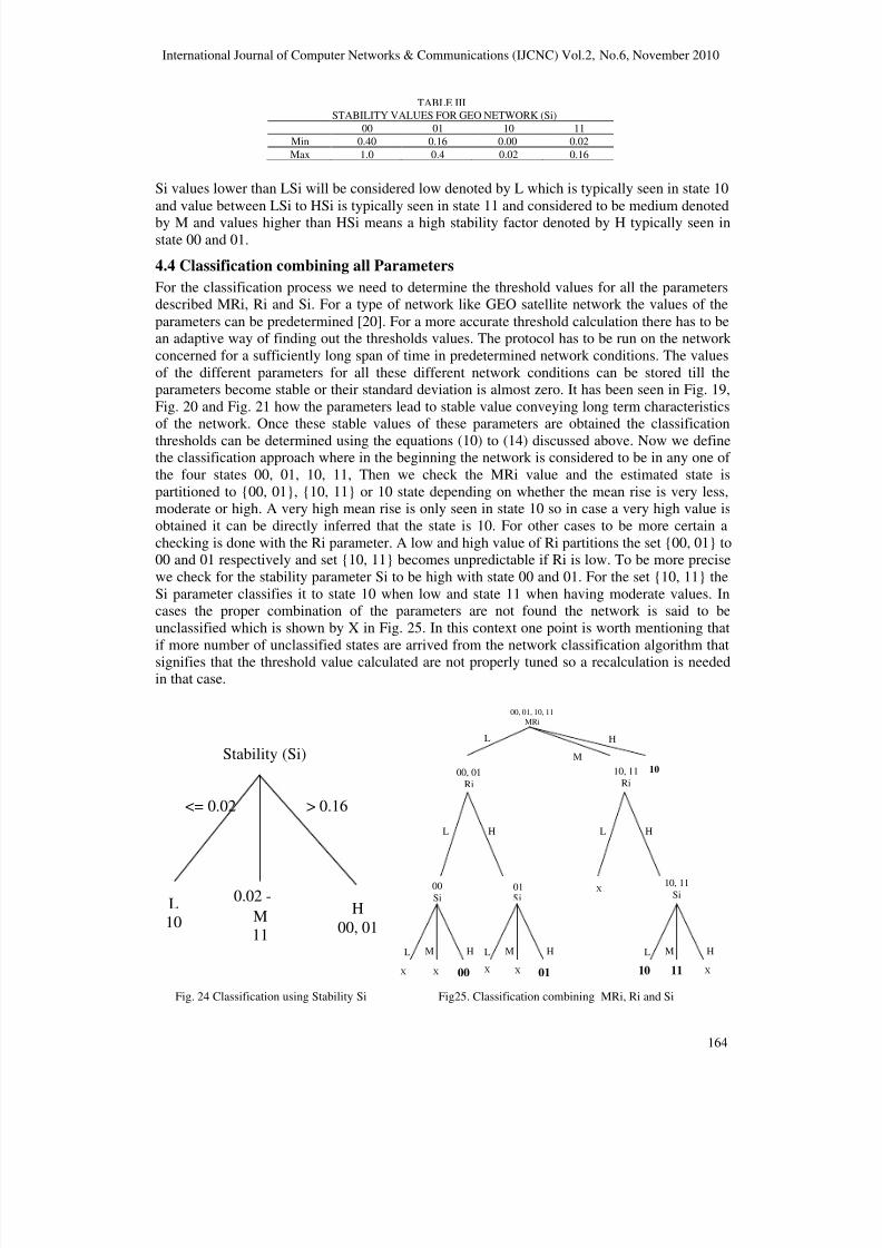
Si values lower than LSi will be considered low denoted by L which is typically seen in state 10and value between LSi to HSi is typically seen in state 11 and considered to be medium denoted

by M and values higher than HSi means a high stability factor denoted by H typically seen instate 00 and 01.

4.4 Classification combining all Parameters

For the classification process we need to determine the threshold values for all the parametersdescribed MRi, Ri and Si. For a type of network like GEO satellite network the values of theparameters can be predetermined [20]. For a more accurate threshold calculation there has to bean adaptive way of finding out the thresholds values. The protocol has to be run on the networkconcerned for a sufficiently long span of time in predetermined network conditions. The valuesof the different parameters for all these different network conditions can be stored till theparameters become stable or their standard deviation is almost zero. It has been seen in Fig. 19,Fig. 20 and Fig. 21 how the parameters lead to stable value conveying long term characteristicsof the network. Once these stable values of these parameters are obtained the classification

thresholds can be determined using the equations (10) to (14) discussed above. Now we definethe classification approach where in the beginning the network is considered to be in any one of the four states 00, 01, 10, 11, Then we check the MRi value and the estimated state ispartitioned to {00, 01}, {10, 11} or 10 state depending on whether the mean rise is very less,moderate or high. A very high mean rise is only seen in state 10 so in case a very high value isobtained it can be directly inferred that the state is 10. For other cases to be more certain achecking is done with the Ri parameter. A low and high value of Ri partitions the set {00, 01} to00 and 01 respectively and set {10, 11} becomes unpredictable if Ri is low. To be more precisewe check for the stability parameter Si to be high with state 00 and 01. For the set {10, 11} theSi parameter classifies it to state 10 when low and state 11 when having moderate values. Incases the proper combination of the parameters are not found the network is said to beunclassified which is shown by X in Fig. 25. In this context one point is worth mentioning thatif more number of unclassified states are arrived from the network classification algorithm thatsignifies that the threshold value calculated are not properly tuned so a recalculation is neededin that case.

10, 11Ri

L H

M

X

00, 01, 10, 11MRi

00, 01Ri

10

00Si

X 00 01 10 11

L M HL M HL M H

L H L H

01 10, 11Si

XXXX

Fig. 24 Classification using Stability Si Fig25. Classification combining MRi, Ri and Si

Stability (Si)

L10 M

11

H00, 01

<= 0.02

0.02 -

> 0.16




165

6. ADAPTIVE MULTI STATE PROACTIVE TCP PROTOCOL

6.1 Brief Working of Adaptive Multi-State Proactive TCP

In this section we introduce an Adaptive Multi State Proactive Transport Protocol, which is anend-to-end solution to improve the throughput performance in satellite networks [15][21]. Theprotocol uses a proactive approach and is composed of new approaches like Proactive SlowStart, Proactive Congestion Avoidance, State based Error Recovery, and State based TimeoutAction algorithms along with traditional TCP algorithms like Fast Retransmit [20]. Thephilosophy of the protocol is that certain statistical parameters of the network can be slowlyadapted for better proactive actions. With a prior knowledge about the characteristic of thenetwork the performance of the protocol can be greatly enhanced specially during challengingenvironments [13][15][21] of high wireless link errors. In Fig. 26 the overall mechanism of theproposed Adaptive Multi-State Proactive TCP scheme is depicted.

The Network State Classification Algorithm is the heart of this Adaptive State based protocol.For every window after the ACKs for all the transmitted packets are received before the start of a new round of packet transfer, Network State Classification is performed which estimates thestate in which the network is presently or an unclassified state using the Network ClassifiactionAlgorithm as described in Fig 31.

The protocol starts with the Proactive Slow Start phase where the slow start threshold is kept athalf the receiver window, the congestion window to one and the state of the protocol is, NoCongestion No Error ie state 00. The receiver window signifies the maximum number of segments the receiver can accommodate. The congestion window is increased by one with eachreceived ACK so that the congestion window doubles every RTT until the slow start thresholdis reached. But the mean RTT is also checked during this phase and if RTT increase for threesuccessive windows [20] is detected the congestion window is reduced by an Adaptive penaltyfactor shown in Fig. 40. After slow start threshold is crossed the protocol moves to the ProactiveCongestion Avoidance phase where it increases the congestion window by 1/cwnd for everyreception of ACK as in traditional Congestion Avoidance Algorithm. Now if anacknowledgment is not received for a transmitted segment within its retransmission timeoutperiod, the timer expires and the algorithm enters the State based Timeout Action phase. Asshown in Fig. 37 here depending on the state of the network the timeout action is taken. If the

state is any among 00, 10 or 11 then the congestion window is reduced to one and ProactiveSlow Start is initiated [18]. If the state is 01 then the congestion window is not reduced and theprotocol remains in Proactive Congestion Avoidance, only the packets not acknowledged areretransmitted.

During the Proactive Congestion Avoidance the mean RTT is checked every time and if anincrease in RTT for three successive congestion windows [20] is detected the congestionwindow is reduced by the adaptive penalty factor using State based Proactive Action Algorithmas shown in Fig. 41. For every window the Network State Classification also predicts the stateof the network.

Now if three duplicate ACKs are received the protocol calls the Fast Retransmit algorithm and aretransmission [18] is done of the lost segment and the protocol moves to the State based ErrorRecovery Algorithm as shown in Fig. 39. In this phase if the protocol is in state 10 or 11 which

signals that the network has some congestion and a packet is not received by the receiver thenthe chance of the packet being lost by congestion is more. So the congestion window is reducedto half and protocol moves to the Proactive Congestion avoidance phase. If the state of thenetwork is 00 then the congestion window is reduced to ¾ of this value. No reduction incongestion window is done when the state of the network is 01 which signifies that the loss iserror initiated. An unclassified state is considered as state 11 because in state 11 all actions areconservative and this prevents from performance degradation during unsuccessful classification.The Adaptive Multi State Proactive TCP Protocol uses some concepts of Proactive TCP [20]Protocol designed by the authors and is best suited to work in high error conditions.




166

6.2 Overall Operation of the Protocol

The overall operation of the protocol can be classified into a Training Phase and an OperationalPhase. During the Training Phase the protocol learns about the characteristics of the network byadapting the statistical parameters and calculates the threshold parameters, which are eventuallyused for network state classification. The basic algorithm is presented below in Fig. 27.

Before the Adaptive Multi State Algorithm can be used it is necessary to have the thresholdvalues for the network state classification process. For a particular type of network these valuescan be predetermined where the traffic dynamics are less. For example we have calculated thevalue of the thresholds for a GEO based network in our simulation based experiments with anidea about the ideal RTT value for a GEO satellite which is 550ms[1][2]. With predeterminedthreshold values pertaining to the type of network in which the protocol is supposed to run, thetraining process may be skipped. But for networks, which have a more dynamic pattern of traffic, before the protocol can be used a training of the protocol is necessary to calculate thethreshold values of the parameters. This is a familiarization of the network dynamics to theprotocol under different conditions of congestion and error. The network has to be run throughvarying levels of congestion and corruption so as to create the different network states while theparameters are recorded [23]. In an overview the main algorithms to be used are given below inFig. 27. Basically using the Parameter Adaptation process the data collection will happen

followed by Threshold_Calculation Algorithm to calculate thresholds. These two algorithms arepart of the initial training process

Once the thresholds are obtained, during the protocoloperation the Parameter_Classification Algorithm willbe used to classify the status of the parameters. Afterthe classification of individual parameters theNetwork State Classification Algorithm will predictthe network state. This state prediction will be used indifferent operations of the protocol as discussed later.Training the Protocol has to be done by intentionally

varying the levels of congestion and channel errors so

as to artificially create network conditions similar to

state00, state01, state10 and state11

The parameters MRi, Ri and Si should be calculated

and stored till the values become stable or the

standard deviation of the calculated parameters are

very less using Parameter_Adaptation()

Determination of Threshold values like {LMRi,

HMRi} for MRi parameter,{LRi} for parameter Ri,

and {LSi, HSi} for Si using Algorithm

Threshold_Calculation()

For each Window after all the transmitted packets are

ACKed, the MRi, Ri and Si parameters are updated

and classify the Status of Parameters MRi, Si and Ri

as Low, Medium or High using

Parameter_Classification() Algorithm

Classify the Network States through a hierarchal

checking of the values MRi, Ri and Si according to

Fig. 25 and using Network_State_Classification()

Algorithm

Fig. 26 Flow Start of Adaptive Multi State Proactive TCP Fig. 27 Overall Operation of the Protocol

()

N

Timeout

Elapsed

ndup

o

Proactive SlowStart ()

Duplicated ACKS

Yes

FastRetransmit

ProactiveCongestion

Avoidance ()

State based ErrorRecovery

{01}

State based TimeoutAction ()

{00, 10, 11}




167

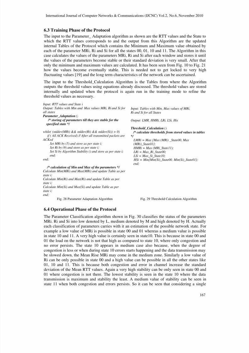
6.3 Training Phase of the Protocol

The input to the Parameter_ Adaptation algorithm as shown are the RTT values and the State towhich the RTT values corresponds to and the output from this Algorithm are the updatedinternal Tables of the Protocol which contains the Minimum and Maximum value obtained byeach of the parameter MRi, Ri and Si for all the states 00, 01, 10 and 11. The Algorithm in thiscase calculates the values of the parameters MRi, Ri and Si after each window and stores it until

the values of the parameters become stable or their standard deviation is very small. After thatonly the minimum and maximum values are calculated. It has been seen from Fig. 10 to Fig. 21how the values become eventually stable. This is needed not to get locked to very highfluctuating values [19] and the long term characteristics of the network can be ascertained.

The input to the Threshold_Calculation Algorithm is the Tables from where the Algorithmoutputs the threshold values using equations already discussed. The threshold values are storedinternally and updated when the protocol is again run in the training mode to refine thethreshold values as necessary.

Input: RTT values and State i

Output: Tables with Min and Max values MRi, Ri and Si for all states

Parameter_Adaptation ()

/* storing of parameters till they are stable for the

specified state */

while( (stddev(MRi) && stddev(Ri) && stddev(Si)) > 0)

if ( All ACK Received) // After all transmitted packets are

ACKed

Set MRi by (5) and store as per state i;

Set Ri by (9) and store as per state i;Set Si by Algorithm Stability () and store as per state i;

end;end;

/* calculation of Min and Max of the parameters */ Calculate Min(MRi) and Max(MRi) and update Table as per

state i;Calculate Min(Ri) and Max(Ri) and update Table as per state i;

Calculate Min(Si) and Max(Si) and update Table as per

state i;

end;

Input: Tables with Min, Max values of MRi,

Ri and Si for all States

Output: LMR, HMRi, LRi, LSi, His

Threshold_Calculation ()

/* calculate thresholds from stored values in tables

*/ LMRi = Max {Max (MRi) _State00, Max(MRi)_State01};

HMRi = Max (MRi_State11); LRi = Max_Ri_State00;

LSi = Max_Si_State10; HSi = Min{Min(Si)_State00, Min(Si)_State01};

end;

Fig. 28 Parameter Adaptation Algorithm Fig. 29 Threshold Calculation Algorithm

6.4 Operational Phase of the Protocol

The Parameter Classification algorithm shown in Fig. 30 classifies the status of the parametersMRi. Ri and Si into low denoted by L, medium denoted by M and high denoted by H. Actuallyeach classification of parameters carries with it an estimation of the possible network state. Forexample a low value of MRi is possible in state 00 and 01 whereas a medium value is possiblein state 10 and 11. A very high value is certainly seen in state10. This is because in state 00 and01 the load on the network is not that high as compared to state 10, where only congestion and

no error persists. The state 10 appears in medium case also because, when the degree of congestion is less or when during state 10 errors starts happening and the data transmission maybe slowed down, the Mean Rise MRi may come in the medium zone. Similarly a low value of Ri can be only possible in state 00 and a high value can be possible in all the other states like01, 10 and 11. This is because both congestion and error in channel increase the standarddeviation of the Mean RTT values. Again a very high stability can be only seen in state 00 and01 where congestion is not there. The lowest stability is seen in the state 10 where the datatransmission is maximum and stability the least. A medium value of stability can be seen instate 11 when both congestion and errors persists. So it can be seen that considering a single




168

parameter, the network can be estimated to be within a set of the network states. When all theseindividual estimations are combined the network state classification can be done using NetworkClassification() algorithm shown in Fig. 31.

Input: MRi, Ri, Si

Output: MRi_Status, Ri_Status, Si_Status

Parameter_Classification () /* Updates status of parameters as low (L), medium (M

) and high (H) */ if(MRi <= LMRi)

MRi_Status = L;elseif(MRi > LMRi && MRi <= HMRi)

MRi_Status = M;elseif(MRi > HMRi)

MRi_Status = H;

if(Ri < LRi)

Si_Status = L;

else Ri_Status = H;

if(Si < LSi)

Si_Status = L;elseif(Si > LSi && Si < HSi)Si_Status = M;

elseif(Si > HSi)

Si_Status = H;end;

Input: MRi_Status, Ri_Status, Si_Status

Output: Network_State

Network_State_Classifiaction ()if (MRi_Status = L)

if (Ri_Status = L)

if (Si_Status = H)

State = 00;else

State = Unclassified;

else

if (Si_Status = H)State = 01;

elseState = Unclassified;

end;

if (MRi_Status = M) {if (Ri_Status = H) {

if(Si_Status = L)

State = 10;else if(Si_Status = M)

State = 11;

}

else

State = Unclassified;return State;

end;

Fig. 30 Parameter Classification Algorithm Fig. 31 Network State Classification Algorithm

7. DESIGN CONSIDERATIONS OF ADAPTIVE MULTI STATE

PROACTIVE TCP

This section describes the internal detail of the proposed protocol and also discusses the

rationale of the specific approach. The section describes the Simulation based experimentswhich have been carried out to analyze in detail how the different protocol related parametersrespond to packet error rates with a view to enhance the performance [13][14] of the protocolunder high error conditions.

7.1 Selective Acknowledgment Scheme

Whenever there is a loss due to duplicate acknowledgment or due to timeout [18], generallytransport protocols transmit all the packets again starting from the point the highestacknowledgment was received if cumulative ACK scheme is used. When multiple packet lossesappear in the same window the repeated transmission of packets already transmitted leads tosome performance degradation [13][16]. So in the Adaptive Multi State Proactive TCPSelective ACK [6] scheme is used, where selectively packets can be retransmitted.

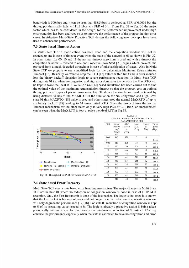
7.2 Effect of Packet Error on Protocol ParametersIn the simulation experiment using scenario of Section7, the Packet Error rates is graduallyincreased from a very low value of 0.0001 to very high value of 0.1 and the total number of Windows, RTT Increase Frequency, DUP ACK Frequency, Timeout Frequency and achievedthroughput is plotted as shown in Table IV. The maximum bandwidth utilization possible foreach connection is 500kbps if they are fairly [11] [10] sharing the 5Mbps of Satellite bandwidthavailable.




169

Fig. 32 shows the total number of windows or in other words rounds [9] which could becompleted within the 500 secs simulation time. It can be seen that as the packet error rateincreases, due to more retransmissions the protocol is able to complete lesser number of roundsof data transfer. This parameter is more useful to visualize the amount of time the protocolkeeps waiting because of an increase in the retransmission timer. In PER of 0.0001 within a 500secs time, 842 rounds could be completed and in PER of 0.1 only 318 rounds could becompleted. This shows why the throughput is degraded as the PER increases.

0

100

200

300

400

500

600

700

800

900

0 0.02 0.04 0.06 0.08 0.1 0.12

PER

N u m b e r o f W i n d o w s

-10

0

10

20

30

40

50

60

70

0 0.02 0.04 0.06 0.08 0.1 0.12

PER

F r e q u e n c y

Fig. 32 Number of Windows vs PER Fig. 35 Timeout_Frequency with PER

0

50

100

150

200

0 0.02 0.04 0.06 0.08 0.1 0.12

PER

F r e q u e n c y

0

100

200

300

400

500

600

0 0.02 0.04 0.06 0.08 0.1 0.12

PER

G o o d p u t ( k

b p s )

Fig. 33 RTT_Increase_Frequency with PER Fig. 36 Goodput (kbps) with PER

0

50

100

150

200

250

300

350

0 0.02 0.04 0.06 0.08 0.1 0.12

PER

F r e q u e n c y

State_based_Timeout_Action()if (RTO expiry)

if (state = 01)

MAXRTO = 2 * IRTT

/* cwnd not changed */ Proactive_Congestion_Avoidance ();

end;

elseif (state = 00| 10 | 11)cwnd = 1;

Proactive_Slow_Start();end;

end;

Fig. 34 Dup_ACK_Frequency Fig. 37 State based Timeout Action

Fig. 33 shows the Frequency of three successive increases in mean RTT values within thesimulation time which triggers a proactive correction of congestion window. As the PERincreases this frequency is seen to reduce because with more errors the amount of datatransmitted by the protocol also reduces. This frequency is important from the fact that witheach such occurrence there is a proactive decrease of the congestion window [20]. Anotherimportant fact which is observed is that, at very high error rates when the amount of datatransmitted is reduced there is an appreciable amount of proactive reduction attributed by error

initiated RTT increase. Fig. 34 shows the frequency of DUP ACK reception with PER and it hasbeen seen that initially the DUP ACK frequency increases with increasing PER and then itreduces since less data being transmitted because of frequent reduction of the congestionwindow during the DUP ACK handling. Fig. 35 shows the frequency of occurrence of timeoutalong with PER. It can be seen that as the PER increases the frequency of timeout increasesappreciably, with no timeout for PER of 0.001, 8 timeouts for PER of 0.01 and 60 timeouts forPER of 0.1. The timeouts are the most expensive events in terms of retransmission and increaseof RTO [18] value leads to the very high degradation [13] of throughput. Fig. 36 shows theachieved goodput [1] with varying PER of the individual connection. The maximum possible




170

bandwidth is 500kbps and it can be seen that 488.5kbps is achieved at PER of 0.0001 but thethroughput drastically falls to 111.2 kbps at a PER of 0.1. From Fig. 32 to Fig. 36 the majorfactor which has to be considered in the design, for the performance improvement under higherror condition has been analyzed so as to improve the performance of the protocol in high errorcases. In Adaptive Multi-State Proactive TCP design the following new concepts have beenused to enhance the performance.

7.3. State based Timeout ActionIn Multi-State TCP a modification has been done and the congestion window will not bereduced to one in case of timeout event when the state of the network is 01 as shown in Fig. 37.In other states like 00, 10 and 11 the normal timeout algorithm is used and with a timeout thecongestion window is reduced to one and Proactive Slow Start [20] begins which prevents theprotocol from a much degraded throughput in case of misclassification of states. Also in MultiState TCP we propose to use a modified logic for the calculation Maximum RetransmissionTimeout [18]. Basically we want to keep the RTO [18] values within limit and in error inducedloss the binary backoff algorithm leads to severe performance reduction. In Multi State TCPduring state 01 i.e. when no congestion and high error dominates the network the Max RTO willbe kept to twice the Ideal RTT value. An ns2 [12] based simulation has been carried out to findthe optimal value of the maximum retransmission timeout so that the protocol gets an optimal

throughput in all types of packet error rates. Fig. 38 shows the simulation result obtained byusing different values of the MAXRTO. In the simulation for No Congestion and High Errorstate 01 this MAXRTO [18] value is used and other states used the normal MAXRTO of up tosix binary backoff [18] leading to 64 times initial RTO. Since the protocol uses the normalTimeout mechanism for the other states only in very high PER of 0.1(-10db) an improvementcan be seen when the MAXRTO is kept at twice the ideal RTT in Fig 38.

0

100

200

300

400

500

600

-40 -30 -20 -10 0

PER(db)

T

h r o

u

g

h p

u t

( k b

p

s )

Normal Timeout MaxRTO = Mean RTT

MAXRTO = 1.5 * Mean RTT MAXRTO = 2 * Mean RTT

MAXRTO = 2 * IRTT

Fig. 38 Throughput vs. PER for values of MAXRTO

7.4. State based Error Recovery

Multi State TCP uses a state based error handling mechanism. The major changes in Multi StateTCP are in state 01 where no reduction of congestion window is done in case of DUP ACKreception. Only the Fast Retransmit is done of the lost packet. The logic is that once it is knownthat the lost packet is because of error and not congestion the reduction in congestion windowwill only degrade the performance [17][18]. For state 00 reduction of congestion window is keptto ¾ of its prevailing value instead to ½. The logic is already a proactive action is being takenperiodically with mean rise for three successive windows so reduction of ¾ instead of ½ mayenhance the performance especially when the state is estimated to have no congestion and error.

TABLE IVSIMULATION RESULT FOR PROTOCOL

PARAMETER VS PERPER Total

number of

Windo

ws

RTT

Increase

Freq

Dup

ACK Freq

Timeo

ut Freq

Throu

ghput (kbps)

.000

1

842 179 0 0

488.5.001 819 138 33 0 473.0.01 675 70 204 8 419.4.02 609 46 277 8 381.1.03 566 46 307 15 318.8.04 533 41 311 17 240.7.05 480 53 285 32 185.0.06 445 35 298 37 192.3.07 381 41 269 51 170.3.08 403 45 293 41 151.3.09 353 41 248 58 118.4.1 318 40 241 60 111.2




171

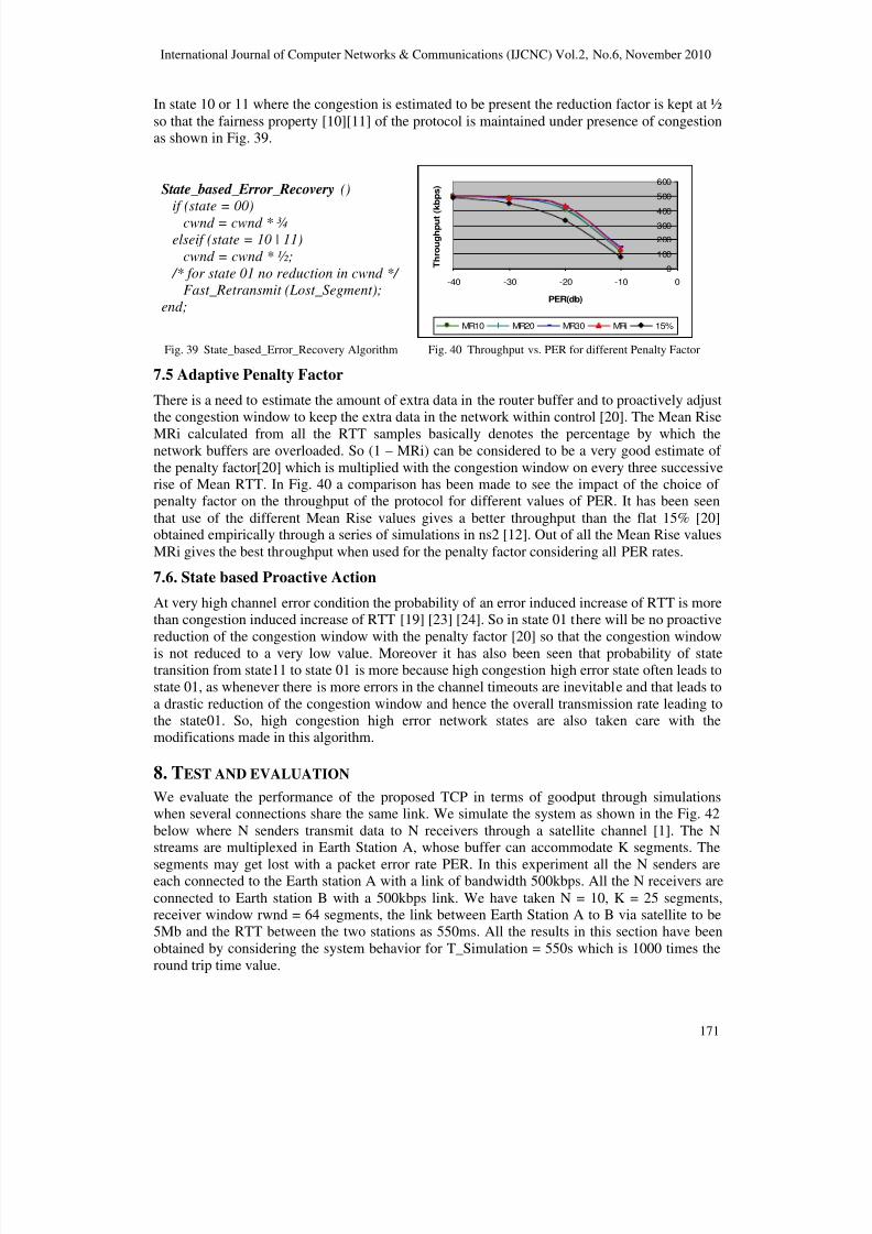
In state 10 or 11 where the congestion is estimated to be present the reduction factor is kept at ½so that the fairness property [10][11] of the protocol is maintained under presence of congestionas shown in Fig. 39.

State_based_Error_Recovery ()

if (state = 00)

cwnd = cwnd * ¾

elseif (state = 10 | 11)

cwnd = cwnd * ½;

/* for state 01 no reduction in cwnd */

Fast_Retransmit (Lost_Segment);

end;

0

100

200

300

400

500

600

-40 -30 -20 -10 0

PER(db)

T h r o u g h p u t

( k b p s )

MR10 MR20 MR30 MRi 15%

Fig. 39 State_based_Error_Recovery Algorithm Fig. 40 Throughput vs. PER for different Penalty Factor

7.5 Adaptive Penalty Factor

There is a need to estimate the amount of extra data in the router buffer and to proactively adjustthe congestion window to keep the extra data in the network within control [20]. The Mean Rise

MRi calculated from all the RTT samples basically denotes the percentage by which thenetwork buffers are overloaded. So (1 – MRi) can be considered to be a very good estimate of the penalty factor[20] which is multiplied with the congestion window on every three successiverise of Mean RTT. In Fig. 40 a comparison has been made to see the impact of the choice of penalty factor on the throughput of the protocol for different values of PER. It has been seenthat use of the different Mean Rise values gives a better throughput than the flat 15% [20]obtained empirically through a series of simulations in ns2 [12]. Out of all the Mean Rise valuesMRi gives the best throughput when used for the penalty factor considering all PER rates.

7.6. State based Proactive Action

At very high channel error condition the probability of an error induced increase of RTT is morethan congestion induced increase of RTT [19] [23] [24]. So in state 01 there will be no proactivereduction of the congestion window with the penalty factor [20] so that the congestion window

is not reduced to a very low value. Moreover it has also been seen that probability of statetransition from state11 to state 01 is more because high congestion high error state often leads tostate 01, as whenever there is more errors in the channel timeouts are inevitable and that leads toa drastic reduction of the congestion window and hence the overall transmission rate leading tothe state01. So, high congestion high error network states are also taken care with themodifications made in this algorithm.

8. TEST AND EVALUATION

We evaluate the performance of the proposed TCP in terms of goodput through simulationswhen several connections share the same link. We simulate the system as shown in the Fig. 42below where N senders transmit data to N receivers through a satellite channel [1]. The Nstreams are multiplexed in Earth Station A, whose buffer can accommodate K segments. The

segments may get lost with a packet error rate PER. In this experiment all the N senders areeach connected to the Earth station A with a link of bandwidth 500kbps. All the N receivers areconnected to Earth station B with a 500kbps link. We have taken N = 10, K = 25 segments,receiver window rwnd = 64 segments, the link between Earth Station A to B via satellite to be5Mb and the RTT between the two stations as 550ms. All the results in this section have beenobtained by considering the system behavior for T_Simulation = 550s which is 1000 times theround trip time value.




172

State_based_Proactive_Action()

if(RTT_Increase_Detected)

if(state = 00 | 10 | 11)

cwnd = cwnd * (1 – MRi) /* for state 01 no change in cwnd */

end;

Fig. 41 State based Proactive Action Algorithm Fig. 42 Simulation Scenario

8.1 Goodput Calculation

Goodput is the effective amount of data delivered through the network [1]. It is a directindicator of network performance. We expect that a good TCP scheme transmit as muchdata as possible, while behaving friendly to other TCP flows in terms of consuming thenetwork resource. In the following graphs shown the throughput of the protocol iscompared to TCP SACK [6] and TCP Vegas [5] in the same test bed of 10 senders

communicating to 10 receivers using a 5Mb bottleneck link via satellite. To artificiallyinduce congestion the bandwidth between Earth Station A and B is stepwise reduced tosee the reaction of the protocol to congestion. Here all ten different connections areconnected to the Earth Station with 500kbps bandwidth each. So the minimumaggregate bandwidth required for all the connections to perform optimally is 5Mbps.Table V shows the goodput of the Multi State TCP along with Vegas [5], TCP SACK [6] andProactive TCP [20]. In Table VI the percentage utilization is shown and it can be seen thatMulti State TCP utilizes 50% bandwidth even in a very high PER of 0.1. Table VII shows theappreciation over its peers and in high error condition the appreciation is 600% over Vegas and800% over SACK. This is a very significant improvement achieved with following graphsshowing the result in Fig. 43, Fig. 44 and Fig. 45.

In Table VIII the Jain’s fairness index [11] calculated from all the 10 connections for differentpacket error rate is shown. It can be seen that all the connections get an almost equal share of bandwidth [10] with a very slow degradation of fairness with increasing PER.

TABLE VIPERCENTAGE BANDWIDTH UTILIZATION

PER Vegas(%)

SACK(%)

ProactiveTCP (%)

MultiStateTCP (%)

0.001 48.92 45.00 90.00 96.200.01 33.74 23.20 64.7 81.700.1 6.98 5.40 17.33 48.99

TABLE V

GOODPUT FOR CONGESTED NETWORK WITH PERPER Vegas

(kbps)SACK(kbps)

ProactiveTCP(kbps)

MultiStateTCP

(kbps)0.001 244.6 225 450 4810.01 168.7 116 323.6 408.50.1 34.9 27 86.67 244.9

TABLE VIIPERCENTAGE APPRECIATION OF MULTI-STATE

TCP OVER ITS PEERS FOR DIFFERENT PERPER Vegas (%) SACK (%) Proactive

TCP (%)0.001 96.64 113.77 6 .880.01 142.14 252.15 26.230.1 601.97 807.37 182.66

TABLE VIIIJain’s Fairness Index for different Packet Error rates

000 0.0001 0.001 0.01 0.1

0.99999 0.999684 0.999415 0.999626 0.998864




173

0

50

100

150

200

250

300

350

400

450

500

-35 -30 -25 -20 -15 -10 -5 0

PER (db)

T h r o u g h p u t ( k b p s )

Vegas SACK Proactive TCP MultiState TCP

0

20

40

60

80

100

-35 -30 -25 -20 -15 -10 -5 0

PER (db)

B a n d w i d t h U t i l i z a t i o n ( % )

Vegas SACK Proactive TCP MultiState TCP

Fig. 43 Throughput for Congested Network with

different PERFig. 44 Percentage Bandwidth Utilization

0

200

400

600

800

1000

-35 -30 -25 -20 -15 -10 -5 0

PER (db)

A p p r e c i a t i o n ( % )

Vegas SACK Proactive TCP

Fig. 45 Multi-State TCP Appreciation in percentage compared to its peers for different PER

9. CONCLUSION

This paper through detailed simulation and analysis of TCP over Satellite Networks hasestablished the fact that multi state network classification is essential to enhance the overallthroughput of the network which is affected equally by congestion and channel noise. Themodelling and analysis as discussed in this paper has proved that the conventional two statenetwork classification devised in classical TCP over wired network is not optimal for satellitebased TCP protocol. So to enhance the performance of TCP protocols over Satellite basedNetworks there is a need for a Multi State representation of network condition by a combinationof the Multi State Network Classification model to be developed which has been explained inthis paper. For the design of such a model simulation based experiments are carried out toanalyze the impact of congestion and error on RTT values. The inferences drawn from the

analysis have been used to evolve a novel Statistical RTT based model which uses a hierarchicaldecision making process for network state classification. This model has been utilized in thedesign of an Adaptive Multi State Proactive Transport Protocol for performance enhancement of satellite based networks. The major causes of performance degradation have been analyzed andthe novel schemes for throughput enhancement have been proposed. The design considerationof the protocol has been discussed thoroughly in this paper and it has been shown how anadaptive mechanism of learning the statistical parameters of a network can help in getting asignificant performance benefit. The Multi–State TCP is seen to outperform substantially overits peers mainly in high error conditions. The most important merit is that the performanceimprovement obtained in this protocol [14] does not need any change in the Routers and allchanges are restricted to the sender and receiver protocol stack [7].

Acknowledgements

Our special thanks to Mr. V.S.Palsule, Deputy Director, Satellite Navigation Application Area,SAC, ISRO, Mr.A.P.Shukla, Head, ACTD and Mr. N.G.Vasantha Kumar, Senior Scientist,ACTD for providing constant encouragement towards the realization of this work.

References[1] Ian F. Akyildiz, Giacomo Morabito, Sergio Palazzo, (2001) “TCP-Peach: A New Congestion

Control Scheme for Satellite IP Networks”, IEEE/ACM TRANSACTIONS ONNETWORKING, VOL. 9, NO. 3, JUNE




174

[2] Ian F. Akyildiz , Xin Zhang, Jian Fang, (2002) “TCP-Peach+: Enhancement of TCP-Peach for

Satellite IP Networks”, IEEE COMMUNICATIONS LETTERS, VOL. 6, NO. 7, JULY

[3] Ozgur B. Akan, Jian Fang, Ian F. Akyildiz, (2004) “TP-Planet: A Reliable Transport Protocol

for InterPlaNetary Internet ”, IEEE/SAC, vol 22, no 2, Feb. 2004, pp 348-61

[4] Jian Fang and Özgür B. Akan,(2004)”Performance of Multimedia Rate Control Protocols in

InterPlaNetary Internet ”, IEEE COMMUNICATIONS LETTERS, VOL. 8, NO. 8, AUGUST

[5] L. S. Brakmo, S. O Malley, L. L. Peterson, (1994) “TCP Vegas: New Techniques for Congestion Detection and Avoidance”, Proc. ACM SIGCOMM 1994, pp. 24-35, October

[6] Mathis, M., J. Mahdavi, S.Floyd, and A.Romanow, (1996) “TCP Selective Acknowledgment

Options”, RFC 2018, April

[7] J. Martin, A. Nilsson, and I. Rhee, (2003) “ Delay-Based Congestion Avoidance for TCP”,IEEE/ACM Transactions on Networking, vol. 11, no. 3, pp. 356–369, June

[8] M. Mathis, J. Mahdavi, (1996) “Forward Acknowledgment: Refining TCP Congestion Control”,Proc. ACM SIGCOMM 1996, pp. 281-292, Aug.

[9] J. Padhye, V. Firoio, D. Towsley, J. Kurose, (2000) “ Modeling TCP Reno Performance: A

Simple Model and Its Empirical Validation”, IEEE/ACM Trans. Networking, Vol. 8, No. 2, pp.133-145, April

[10] S.C. Tsao, Y.C. Lai, and Y.D. Lin, (2007) “Taxonomy and Evaluation of TCP-FriendlyCongestion-Control Schemes on Fairness, Aggressiveness, and Responsiveness”, IEEE Network,November

[11] R. Jain, D. Chiu, and W. Hawed, (1984) “ A quantitative measure of fairness and discrimination

for resource allocation in shared computer systems”, DEC, Res. Rep.TR-301,

[12] UCB/LBNL/VINT Network Simulator [Online]. Available: http://www.isi.edu/nsnam/ns/

[13] T.V.Lakshman and U.Madhow, (1997) “The performance of TCP/IP for networks with high

bandwidth-delay products and random loss”, IEEE/ACM Trans. Networking, vol. 5, June

[14] Injong Rhee and Lisong Xu, (2007) “ Limitations of Equation-based Congestion Control”, IEEE/ACM Trans. Networking, June

[15] C. Metz, (1999) “TCP over satellite the final frontier ”, IEEE Internet Compuingting., pp. 76–80,Jan. /Feb

[16] C. Partridge and T. J. Shepard, (1997) “TCP/IP performance over satellite links”, IEEE NetworkMagazine., pp. 44–49, Sept-Oct.

[17] W. Stevens, (1994) “TCP/IP Illustrated” Addison-Wesley, vol.1

[18] V. Jacobson, (1988) “Congestion avoidance and control,” in Proc. ACM SIGCOMM

[19] Ravi.S.Prasad, “On the Effectiveness of Delay-Based Congestion Avoidance “

[20] Mohanchur Sarkar, K.K.Shukla, K.S.Dasgupta, (2010) “A Proactive Transport Protocol forPerformance Enhancement of Satellite based Networks” in (IJCA) International Journal of Computer Applications, Vol 1, Number16, pp. 114-121, Feb

[21] M. Allman, (2000), “Ongoing TCP research related to satellites”, RFC 2760, Feb.

[22] Jiang Wu, Hosam El-Ocla , (2004) “TCP Congestion Avoidance Model with Congestive Loss”,

in Proceedings 12

th

IEEE International Conference,2004, Vol 1 , pp. 3-8[23] Abhishek Murthy, (2006) “Correlation Coefficient based Loss Differentiation Algorithm

(CCLDA) for TCP vis-à-vis traditional LDAs”, 4th Conference on Research and Development

[24] S. Biaz, (2003) “Is the round-trip time correlated … flight” Internet Measurement Conference

Date post:	10-Apr-2018
Category:	Documents
Upload:	aircc-ijcnc
View:	218 times
Download:	0 times

Network State Classification Based on the Statistical Properties of RTT for an Adaptive Multi-State...

Documents