1

Networking Programmable Logic Controllers:Pneumatic Cylinder Modelling and Control

Diogo Miguel Correia dos SantosInstituto Superior Tecnico / UTL, Lisbon, Portugal

Abstract—Building real world reliable and robust systemsnowadays is usually associated to the use of Programmable LogicControllers (PLCs). These devices are modular digital computersthat allow using a large variety, and number, of electrical inputand/or output interfaces. The mechanical, hardware and softwareare designed to handle continuous operation in environmentsoverwhelmed with electromagnetic and mechanical noise. Thesecharacteristics make PLCs ideal for usage within industrialenvironments: travel industry, aerospace, food industry andtextile industry, or any other area with systems operated bycontrollable machines. However, as technology advances, thesystems to be controlled become more complex. As a result,networking PLCs is becoming not just simply an interest, butan actual requirement. PLC network systems profit greatly fromhaving a Supervisory Control and Data Acquisition (SCADA)system to supervise them. This system is generally composedof a remote monitoring and operation software application thatallows observation and control of the industrial process. Withthe level of detailed surveillance and control capabilities thatSCADA provides, the security and productivity of the systemboth increase. The objective of this thesis was to design a remotemonitoring and operation interface for a physical setup withequipment that could be controlled by Programmable LogicControllers.

The available equipment for the construction of the physicalsetup was a set of pneumatic components. Pneumatics is asection of technology with a whole theory behind it, and so, itwas necessary to get briefly acquainted with that theory beforeproceeding with any experiments. The assembled system wasformed by a double acting cylinder, a double solenoid valve,single direction speed controllers, and a compressor. The purposeof this setup was to be able to control the position of the cylinderthrough the remote monitoring and operation interface.

The PLC model used accepted external communications (tobe more precise, an Ethernet/IP based protocol named Modbus)while in operating mode, but only under specific conditions.A dedicated study was indispensable to ascertain the exactcircumstances under which the PLC allowed external commands,as well as to find out their structure.

I. INTRODUCTION

A. Motivation

With the recent advances in the world of automation,especially in the industrial field, the use of modular digitalcomputers has become vital. These devices can withstandvery harsh environments, and offer a simple, wide variety ofinput/output capabilities that would otherwise be achieved withlarge, complex relay circuits. Throughout this thesis they willbe addressed as Programmable Logic Controllers (PLCs) [1],since it is the name they are commonly known for in industrialautomation.

Naturally, to control numerous machines effectively, it isusually desirable to have some means of interconnectionbetween the PLCs that are in charge of the control of suchmachines. In most cases, for efficiency purposes, severalnetworks are required, where PLCs are connected to each otherthrough physical or wireless communication channels. Thesesetups are common when the PLCs are responsible for thestate of the system (or the state of a subsystem) as a whole,rather than the state of just one machine. Nowadays, most PLCnetworks are composed of Ethernet/IP infrastructures, mainlydue to the speed of data transmission that Ethernet provides,as well as the simplicity of the message framing protocols thatwere developed for those structures.

The domain of interest in this thesis lies within the DiscreteEvent Systems (DES). To implement a given DES, there arethree typical modelling methodologies [2]: use a GRAFCET(otherwise known as Sequentional Function Chart, SFC), usea Petri Net, or use an Automaton. The first choice, GRAFCET,is actually a graphical programming language, one of thefive languages defined by IEC 61131-3 that can be used toprogram PLCs [3]. Therefore, its implementation in PLCsis straightforward, as the only requirement is the knowledgeof the language. The second choice, Petri Net, has moremodelling capacity than GRAFCET, but it does not have adirect implementation in PLCs, consequently demanding someindirect solution, or the help of software that can interpret PetriNets on its own. However, for Petri Nets, there are severalanalysis methods available that provide a lot of insight aboutthe system. This is a great advantage compared to GRAFCET,since the latter is very limited in analysis methods. Lastly, theautomaton is a self-operating machine, built explicitly for thedesired system.

Whichever choice is made for the modelling of the DES,if the intended purpose of the system falls within industrialautomation, then a model of control for the system, alongwith an efficient User Interface, are both also necessary.Presently, industries rely on Supervisory Control And DataAcquisition (SCADA) [4] systems for control access andremote monitoring of their machinery. Simply put, they are themodern example of Supervised systems, resorting to softwaredeveloped for monitoring and control through the acquisitionof coded signals from the equipment. The frequent associationbetween SCADA systems and PLCs is that usually the PLCsprovide the signals to be interpreted by the SCADA softwareas a specific state of the machines they are responsible for,and in turn, the SCADA system sends back signals that areinterpreted by the PLCs as commands for those machines.

2

Additionally, SCADA systems are also designed to grantfeatures like failure detection, isolation capacity, and providinghistorical information about previous activity of the controlledsystem [2].

The goal of this thesis is to approach and solve efficientlyan academic, industrial automation problem: the design andimplementation of a SCADA system to oversee and control aDiscrete Event System. In order to accomplish this, it willbe necessary to model and create an industrial resemblingsetup, resorting to modelling dynamics tools. This setup isgoing to be controlled by a PLC network, using a specificmessage framing protocol designed for Ethernet/IP networksthat is currently being used in modern industries: Modbus [5].The available theory on modelling DES may also be useful.The work can thus be summarized into two main steps:

- Assembling a small physical setup that allows remotemonitoring and operation, in which the equipment can becontrolled by Programmable Logic Controllers. Specifically,the PLC will command pneumatic actuators.

- Designing the remote monitoring and operation interfacefor the physical setup. The PLC model available to actuatethe system is Schneider Premium TSX P57 [6]. The commu-nications protocol of the network connecting the Supervisedsystem to the PLC is Modbus.

B. Related Work

The work Modeling and Identification of Pneumatic Actua-tors [7] presents an in-depth study of a pneumatic actuator. Itoffers both a defined physical model and a possible design ofa non-linear parametric model for it. This knowledge is thenapplied in the control of a humanoid robot. Categorically, [7]provides useful information about the principles of the cylindermodel, and inclusively mentions a particularly interestingphenomenon: stiffness. It is commonly known as the resistanceof a body to deformation by influence of external forces, butin pneumatic actuators such as the cylinders, it may be usedas a form of control. During the empirical work of this thesis,a two-chamber cylinder like the one mentioned in [7] willbe used, and therefore, both the information and the describedphenomenon are substantial contributions worth exploring.

Method for communicating among a plurality of pro-grammable logic controllers each having a DMA controller [8]discusses a method for communicating among several Pro-grammable Logic Controllers, all coupled to a common com-munications bus (serial). Many of the concerns that need tobe approached in the method described in [8], are equiv-alently present in this thesis. However, the creation of X-Way communication, and the fact that it is compliant with theProgrammable Logic Controllers used throughout this thesis,greatly simplifies these issues.

C. Problem Formulation

The objectives of this thesis, described in I-A, requiresolving two problems. The first one concerns the physicalsetup, whereas the second is related to communications. It isknown beforehand that the available equipment for the setup

consists of a kit 1 of pneumatic cylinders and valves 2. Theproposed strategy for the usage of these components is tocreate a simple system in which the position of a doubleacting cylinder3 is measured and controlled. The need to takemeasurements leads to the necessity of a proper sensor. Asfor the control, the intent is to actuate one or more valves, tomove the cylinder to a desired position. The actuation will beperformed by a PLC.

Ideally, the assembled setup would have a Network com-posed of two PLCs. One of them would receive measurements,and the other would command the actuation based on thosemeasurements. The specifications of the available PLC model( [6]) indicate that the inter-communications are compliantwith a specific Ethernet/IP protocol, Modbus ( [5]). Thiswill be the communications protocol used in the Network.However, the PLC model does not have input analog cards.For that reason, it is suggested that an Arduino is used instead,to receive the measurements. The Arduino will be able to sendthe measurements via Ethernet with the use of an Ethershield.Finally, it is also expected that the Network can be monitored,and the system controlled, through a remote monitoring andoperation station.

D. Thesis OutlineSection II provides detailed information about the hardware

of modern Programmable Logic Controllers (PLCs).Section III presents theory regarding Pneumatics. Specifi-

cally, it emphasizes on the pneumatic cylinder model, sinceit illustrates the actual cylinder used in the experiments ofthe dissertation. It also offers an overview of the full setup,designed to be controlled by PLCs, and explains in detail threedifferent methods suggested to perform the position control ofthe cylinder.

Section IV summarizes the most relevant experiments con-ducted throughout the dissertation, and their respective results.This Section is divided in two parts: the first regarding thetheoretical model of the pneumatic cylinder, and the secondconcerning the empirical model. The first experiment showssome results regarding computer simulations of the cylindermodel, intended for use in the real system. Based on thoseresults, an approximation for the system is proposed. Thesecond experiment represents the chosen application for theavailable hardware and software: position control of the doubleacting cylinder. The results of the empirical system includeStep response, Calibration methods, and Closed-loop.

Section V is a conclusion of the developed work, as wellas its contributions.

II. PROGRAMMABLE LOGIC CONTROLLERS

Section II addresses the subject of Programmable LogicControllers (PLCs), which form the central part of the envis-aged setup of the dissertation. The specific PLC model usedin the dissertation is briefly introduced in this section.

1https://www.sjf.tuke.sk/kvtar/2/files/PNEU200.pdf2http://www.datasheetarchive.com/dl/Datasheets-UD9/DSARS0040963.pdf3https://www.smc.eu/portal ssl/WebContent/digital catalog 2/jsp/view

product configurator.jsp?dc product id=36559&part number=cd85n20&filter type=dc search filter&sub filter type=partnumber&filter value=cd85n20

3

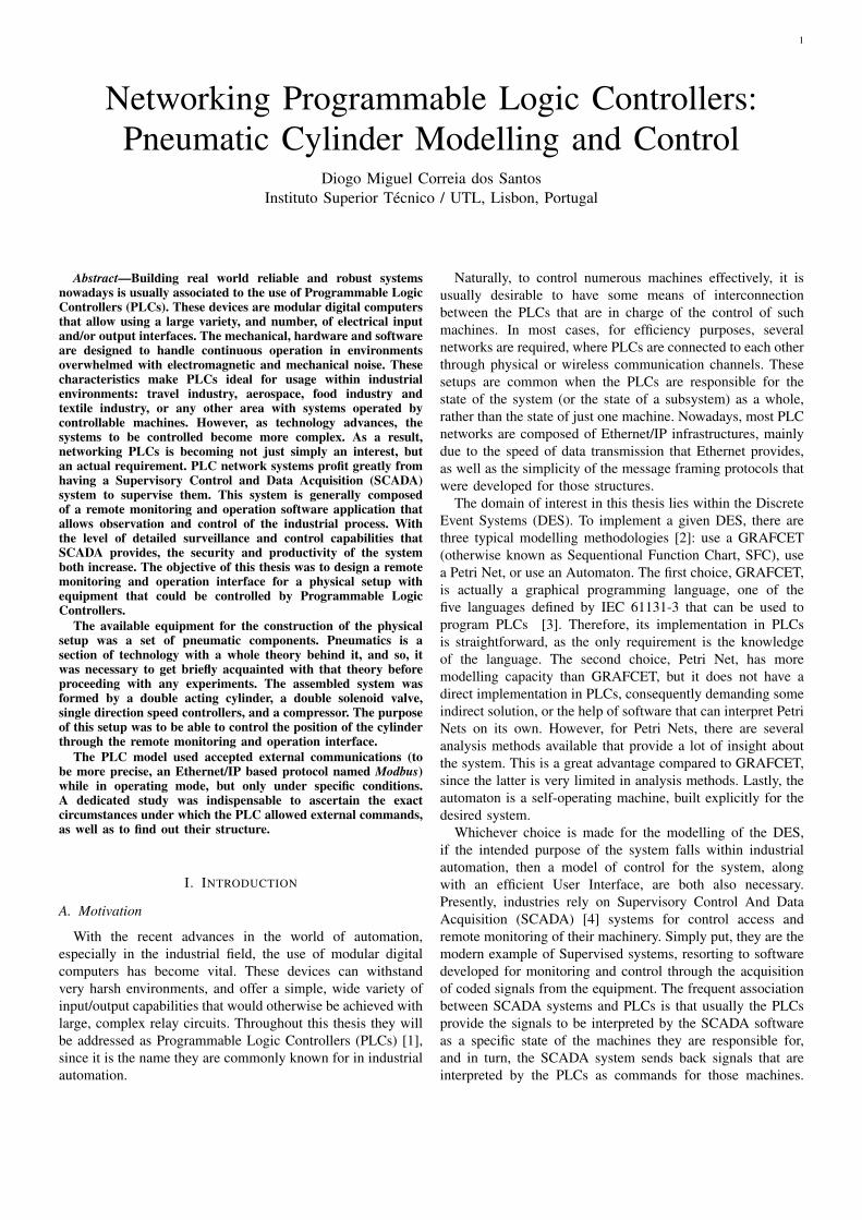
(a) (b)Fig. 1. PLC TSX P57, picture of real model (a) and virtual representation inUnity Pro (b)

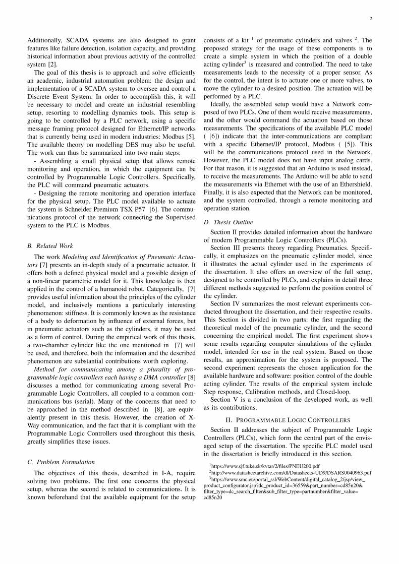
Fig. 2. Real Setup: communications sequence

A. Programmable Logic Controllers

The model at our disposal for this dissertation is Schneider’sTSX P57 Premium [6]. Figure 1 displays both the real model,and its virtual representation in the software where the PLCis programmed, Unity Pro.

This model has a rack with five slots. The CPU model (P572634M) and the Ethernet module (ETY Port) are pluggedinto slots ’0’ and ’1’, respectively, although physically theyare a single hardware piece. The Ethernet module accepts aconnection to a TCP/IP network with X-WAY UNI-TE andModbus messaging facility on a TCP/IP profile, but it mustbe configured in Unity Pro to do so. By default, the projectbuilt in Unity Pro must be loaded to the PLC via RS232/RS485connection. The first serial port on the CPU module is usedfor this effect.

The Inputs module (DEY 16D2) is plugged into slot ’2’.Usually, the signals received by this module dictate what ac-tions the PLC will perform, based on how it was programmed.

The Outputs module (DSY 16T2) is plugged into slot ’4’.The signals transmitted by this module are responsible for theactuation of the machines they are connected to.

III. SYSTEM PROCESS AND CONTROL

The next section describes all the components of the phys-ical setup assembled and the methodology used to controlit. The goal of the experiment is to control the position ofa double acting cylinder, using a pneumatic actuating valve,which will be switching states according to the commandsgiven by a PLC. A sensor will also be necessary, to measurethe current position of the head of the cylinder, and send thesevalues to an Arduino.

A. Closed loop System Overview

The empirical system will follow the communications se-quence shown in figure 2. This figure also displays thefunctions that the Actuator and the Sensor will be performing.Explicitly, the PLC will be controlling the actuation of twovalves, affecting the air flow in and out of the chambers of adouble acting cylinder. This flow will make the cylinder move

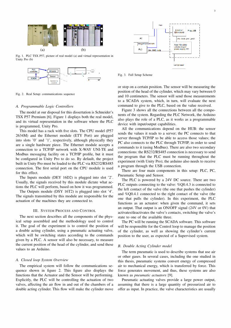
Fig. 3. Full Setup Scheme

or stop on a certain position. The sensor will be measuring theposition of the head of the cylinder, which may vary between 0and 10 centimeters. The sensor will send those measurementsto a SCADA system, which, in turn, will evaluate the nextcommand to give to the PLC, based on the value received.

Figure 3 shows all the connections between all the compo-nents of the system. Regarding the PLC Network, the Arduinoalso plays the role of a PLC, as it works as a programmabledevice with input/output capabilities.

All the communications depend on the HUB: the sensorsends the values it reads to a server; the PC connects to thatserver through TCP/IP to be able to access those values; thePC also connects to the PLC through TCP/IP, in order to sendcommands to it (using Modbus). There are also two secondaryconnections: the RS232/RS485 connection is necessary to sendthe program that the PLC must be running throughout theexperiment (with Unity Pro); the arduino also needs to receivea program through the USB connection.

There are four main components in this setup: PLC, PC,Pneumatic Setup and Sensor.

The PLC is powered by a 24V DC source. There are twoPLC outputs connecting to the valve: %Q0.4.3 is connected tothe left contact of the valve (the one that pushes the cylinder)and %Q0.4.1 connected to the right contact of the valve (theone that pulls the cylinder). In this experiment, the PLCfunctions as an actuator: when given the command, it setsan output. That output is an ON/OFF signal (24V or 0V) thatactivates/deactivates the valve’s contacts, switching the valve’sstate to one of the available three.

The PC will be running the SCADA software. This softwarewill be responsible for the Control loop to manage the positionof the cylinder, as well as showing the cylinder’s currentposition to the user, as expected of a Supervised system.

B. Double Acting Cylinder model

The term pneumatic is used to describe systems that use airor other gases. In several cases, including the one studied inthis thesis, pneumatic systems convert energy of compressedair to mechanical energy, which is transferred by force. Thisforce generates movement, and thus, these systems are alsoknown as pneumatic actuators [9].

Pneumatic actuating valves provide a large power output,assuming that there is a large quantity of pressurized air tooffer as input. In practice, the valve characteristics are usually

4

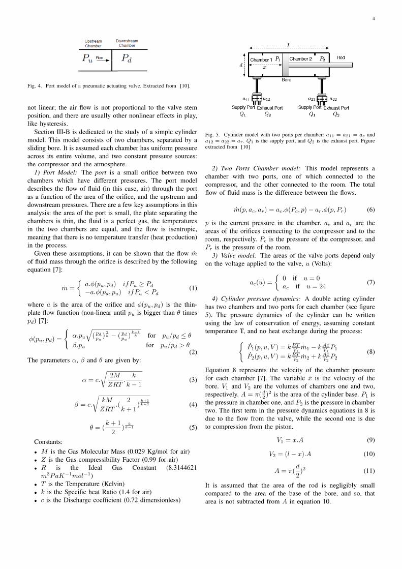
Fig. 4. Port model of a pneumatic actuating valve. Extracted from [10].

not linear; the air flow is not proportional to the valve stemposition, and there are usually other nonlinear effects in play,like hysteresis.

Section III-B is dedicated to the study of a simple cylindermodel. This model consists of two chambers, separated by asliding bore. It is assumed each chamber has uniform pressureacross its entire volume, and two constant pressure sources:the compressor and the atmosphere.

1) Port Model: The port is a small orifice between twochambers which have different pressures. The port modeldescribes the flow of fluid (in this case, air) through the portas a function of the area of the orifice, and the upstream anddownstream pressures. There are a few key assumptions in thisanalysis: the area of the port is small, the plate separating thechambers is thin, the fluid is a perfect gas, the temperaturesin the two chambers are equal, and the flow is isentropic,meaning that there is no temperature transfer (heat production)in the process.

Given these assumptions, it can be shown that the flow mof fluid mass through the orifice is described by the followingequation [7]:

m =

a.φ(pu, pd) ifPu ≥ Pd−a.φ(pd, pu) ifPu < Pd

(1)

where a is the area of the orifice and φ(pu, pd) is the thin-plate flow function (non-linear until pu is bigger than θ timespd) [7]:

φ(pu, pd) =

α.pu

√( pdpu )

2k − ( pdpu )

k+1k for pu/pd ≤ θ

β.pu for pu/pd > θ(2)

The parameters α, β and θ are given by:

α = c.

√2M

ZRT.k

k − 1(3)

β = c.

√kM

ZRT.(

2

k + 1)

k+1k−1 (4)

θ = (k + 1

2)

kk−1 (5)

Constants:• M is the Gas Molecular Mass (0.029 Kg/mol for air)• Z is the Gas compressibility Factor (0.99 for air)• R is the Ideal Gas Constant (8.3144621m3PaK−1mol−1)

• T is the Temperature (Kelvin)• k is the Specific heat Ratio (1.4 for air)• c is the Discharge coefficient (0.72 dimensionless)

Fig. 5. Cylinder model with two ports per chamber: a11 = a21 = ac anda12 = a22 = ar . Q1 is the supply port, and Q2 is the exhaust port. Figureextracted from [10]

2) Two Ports Chamber model: This model represents achamber with two ports, one of which connected to thecompressor, and the other connected to the room. The totalflow of fluid mass is the difference between the flows.

m(p, ac, ar) = ac.φ(Pc, p)− ar.φ(p, Pr) (6)

p is the current pressure in the chamber. ac and ar are theareas of the orifices connecting to the compressor and to theroom, respectively. Pc is the pressure of the compressor, andPr is the pressure of the room.

3) Valve model: The areas of the valve ports depend onlyon the voltage applied to the valve, u (Volts):

ac(u) =

0 if u = 0ac if u = 24

(7)

4) Cylinder pressure dynamics: A double acting cylinderhas two chambers and two ports for each chamber (see figure5). The pressure dynamics of the cylinder can be writtenusing the law of conservation of energy, assuming constanttemperature T, and no heat exchange during the process:

P1(p, u, V ) = kRTV1m1 − kAxV1

P1

P2(p, u, V ) = kRTV2m2 + kAxV2

P2(8)

Equation 8 represents the velocity of the chamber pressurefor each chamber [7]. The variable x is the velocity of thebore. V1 and V2 are the volumes of chambers one and two,respectively. A = π(d2 )2 is the area of the cylinder base. P1 isthe pressure in chamber one, and P2 is the pressure in chambertwo. The first term in the pressure dynamics equations in 8 isdue to the flow from the valve, while the second one is dueto compression from the piston.

V1 = x.A (9)

V2 = (l − x).A (10)

A = π(d

2)2 (11)

It is assumed that the area of the rod is negligibly smallcompared to the area of the base of the bore, and so, thatarea is not subtracted from A in equation 10.

5

5) Force dynamics: There are four different forces consid-ered in the two-chamber model that affect the position variable,x [10]. The first is the force obtained from the difference ofpressures in both chambers:

F1 = (P1 − P2).A (12)

The second force corresponds to the sum of the dynamicfriction and viscous forces:

F2 = sgn(x).kd + kv.x (13)

The third force, F3, is the external force applied to the piston.The fourth force is the static friction, which counterbalancesall other forces up to a threshold ks:

F4 =

−(F1 + F2 + F3), if |F1 + F2 + F3| < ks0, otherwise

(14)By applying the Newton’s law, the model dynamics equationis obtained [10]:

x =1

m.(F1 + F2 + F3 + F4) (15)

6) Computer Simulations: It is assumed that the modelis frictionless, moving a load of constant mass, m. Thishypothesis nullifies all forces except F1, the one derived fromthe difference of chamber pressures. The set of simulationequations, already discretized, is the following [10]:

xt =A

m.(P1(t)− P2(t)) (16)

xt+δ = xt + xt.δ (17)

xt+δ = xt + xt.δ +1

2xt.δ

2 (18)

m1(t) = a11(t).φ(Pc, P1(t)) + a12(t).φ(Pr, P1(t)) (19)

m2(t) = a21(t).φ(Pc, P2(t)) + a22(t).φ(Pr, P2(t)) (20)

P1(t) = kRTm1(t)−AxtP1(t)

xtA(21)

P2(t) = kRTm2(t) +AxtP2(t)

(l − xt)A(22)

P1(t+ δ) = P1(t) + P1(t)δ (23)

P2(t+ δ) = P2(t) + P2(t)δ (24)

The process is a discretization in time, with a small time-step δ ( [10]). Equations 16, 17, and 18 correspond to theacceleration, velocity and position of the bore, respectively.Pressures P1 and P2, as well as the position xt and the velocityxt are all state variables. Once they are updated, the chamberpressure variables are computed (equations 19 through 24).The variables a11 and a21 are the areas of the orifices of thevalve that receive air from the compressor, whereas a12 anda22 are the areas of the exhaust ports of the valve. Pc and Prare the pressures of the compressor and the room, respectively.

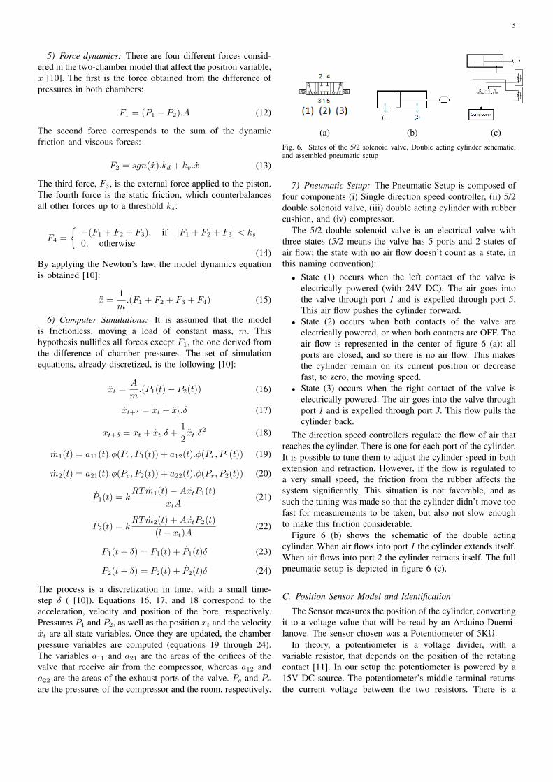
(a) (b) (c)Fig. 6. States of the 5/2 solenoid valve, Double acting cylinder schematic,and assembled pneumatic setup

7) Pneumatic Setup: The Pneumatic Setup is composed offour components (i) Single direction speed controller, (ii) 5/2double solenoid valve, (iii) double acting cylinder with rubbercushion, and (iv) compressor.

The 5/2 double solenoid valve is an electrical valve withthree states (5/2 means the valve has 5 ports and 2 states ofair flow; the state with no air flow doesn’t count as a state, inthis naming convention):• State (1) occurs when the left contact of the valve is

electrically powered (with 24V DC). The air goes intothe valve through port 1 and is expelled through port 5.This air flow pushes the cylinder forward.

• State (2) occurs when both contacts of the valve areelectrically powered, or when both contacts are OFF. Theair flow is represented in the center of figure 6 (a): allports are closed, and so there is no air flow. This makesthe cylinder remain on its current position or decreasefast, to zero, the moving speed.

• State (3) occurs when the right contact of the valve iselectrically powered. The air goes into the valve throughport 1 and is expelled through port 3. This flow pulls thecylinder back.

The direction speed controllers regulate the flow of air thatreaches the cylinder. There is one for each port of the cylinder.It is possible to tune them to adjust the cylinder speed in bothextension and retraction. However, if the flow is regulated toa very small speed, the friction from the rubber affects thesystem significantly. This situation is not favorable, and assuch the tuning was made so that the cylinder didn’t move toofast for measurements to be taken, but also not slow enoughto make this friction considerable.

Figure 6 (b) shows the schematic of the double actingcylinder. When air flows into port 1 the cylinder extends itself.When air flows into port 2 the cylinder retracts itself. The fullpneumatic setup is depicted in figure 6 (c).

C. Position Sensor Model and Identification

The Sensor measures the position of the cylinder, convertingit to a voltage value that will be read by an Arduino Duemi-lanove. The sensor chosen was a Potentiometer of 5KΩ.

In theory, a potentiometer is a voltage divider, with avariable resistor, that depends on the position of the rotatingcontact [11]. In our setup the potentiometer is powered by a15V DC source. The potentiometer’s middle terminal returnsthe current voltage between the two resistors. There is a

6

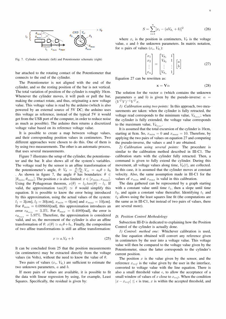
Fig. 7. Cylinder schematic (left) and Potentiometer schematic (right)

bar attached to the rotating contact of the Potentiometer thatconnects to the end of the cylinder.

The Potentiometer is not aligned with the end of thecylinder, and so the resting position of the bar is not vertical.The total variation of position of the cylinder is roughly 10cm.Whenever the cylinder moves, it will push or pull the bar,making the contact rotate, and thus, originating a new voltagevalue. This voltage value is read by the arduino (which is alsopowered by an external source of 5V DC; the arduino usesthis voltage as reference, instead of the typical 5V it wouldget from the USB port of the computer, in order to reduce noiseas much as possible). The arduino then returns a discretizedvoltage value based on its reference voltage value.

It is possible to create a map between voltage values,and their corresponding position values in centimeters. Twodifferent approaches were chosen to do this. One of them isby using two measurements. The other is an automatic process,that uses several measurements.

Figure 7 illustrates the setup of the cylinder, the potentiome-ter and the bar. It also shows all of the system’s variables.The voltage read by the sensor is an affine transformation ofthe potentiometer’s angle, θ: Vθ = θ−θ0

θ1−θ0 .Vcc = a0θ + b0. As shown in figure 7, the angle θ has boundaries: θ ∈[θmin, θmax]. The position x is also limited: x ∈ [xmin, xmax].Using the Pythagorean theorem, x(θ) = l2.tan(θ) − l1. Ifvalid, the approximation tan(θ) ' θ would simplify thisequation. It is possible to know the error being introducedby this approximation, using the actual values of the system:l1 = 3[cm], l2 = 30[cm], xmin = 0[cm] and xmax = 10[cm].For θmin = 0.099668[rad], this approximation introduces anerror eθmin = 3.3%. For θmax = 0.4089[rad], the error iseθmax = 5.97%. Therefore, the approximation is consideredvalid, and so, the movement of the cylinder is also an affinetransformation of θ: x(θ) ' a1θ+b1. Finally, the compositionof two affine transformations is still an affine transformation:

x ' a.Vθ + b (25)

It can be concluded from 25 that the position measurements(in centimeters) may be extracted directly from the voltagevalues (in Volts), without the need to know the value of θ.

Two pairs of values (xi, Vθi ) are sufficient to estimate thetwo unknown parameters, a and b.

If more pairs of values are available, it is possible to fitthe data with linear regression by using, for example, LeastSquares. Specifically, the residual is given by:

S =

n∑i=1

[xi − (aVθi + b)]2 (26)

where xi is the position in centimeters, Vθ is the voltagevalue, a and b the unknown parameters. In matrix notation,for n pairs of values (xi, Vθi ):

x1x2...xn

=

Vθ1 1Vθ2 1

......

Vθn 1

[ab

](27)

Equation 27 can be rewritten as:

x = Vα (28)

The solution for the vector α (which contains the unknownparameters a and b) is given by the pseudo-inverse: α =(V TV )−1V Tx.

1) Calibration using two points: In this approach, two mea-surements are taken: when the cylinder is fully retracted, thevoltage read corresponds to the minimum value, Vθmin

; whenthe cylinder is fully extended, the voltage value correspondsto the maximum value, Vθmax

.It is assumed that the total excursion of the cylinder is 10cm,

starting at 0cm. So, xmin = 0 and xmax = 10. Therefore, byapplying the two pairs of values on equation 27 and computingthe pseudo-inverse, the values a and b are obtained.

2) Calibration using several points: The procedure issimilar to the calibration method described in III-C1. Thecalibration starts with the cylinder fully retracted. Then, acommand is given to fully extend the cylinder. During thismovement, all voltage values along time, Vθ(t), are collected.In this case, it is assumed that the cylinder moves at constantvelocity. Also, the same assumption made in III-C1 for thevalues of xmin and xmax is valid in this calibration.

The data gathered can be represented by a graph startingwith a constant value until time t1, then a slope until timet2, and again a constant value thereafter. Identifying t1 andt2 allows using the least squares line fit (the computations arethe same as in III-C1, but instead of two pairs of values, thereare several more).

D. Position Control Methodology

Subsection III-D is dedicated to explaining how the PositionControl of the cylinder is actually done.

1) Control: method one: Whichever calibration is used,the line equation obtained will convert any reference givenin centimeters by the user into a voltage value. This voltagevalue will then be compared to the voltage value given by thePotentiometer, since the latter corresponds to the cylinder’scurrent position.

The position x is the value given by the sensor, and thereference xref is the value given by the user in the interface,converted to voltage value with the line equation. There isalso a small threshold value ε, to allow the acceptance of asmall window of values of x close to xref . When the condition|x− xref | ≤ ε is true, x is within the accepted threshold, and

7

so a command to turn off the valve is issued. Otherwise, ifthe position x is smaller than xref − ε, the left contact of thevalve is turned on, and the right contact is turned off, so thatthe cylinder will be pushed. If x is bigger than xref + ε, theright contact is turned on, and the left contact turned off, sothe cylinder will pull back.

2) Control: method two: The following control method isa predictive algorithm. The goal of this method is to estimatethe value of the next sample, x(n + 1), at a given instant n.If the value of that sample falls within a certain range of thereference, the command to stop the valves is issued and thecontrol loop ends. In other words, the purpose of this methodis to stop the cylinder when it is estimated that it will reach thedesired position, as opposed to giving that command only afterthe control loop as received the measurement and verified thatthe desired position has been reached. Since the informationis available, this predictive control method uses the knowledgeof both the current sample and the previous one.

Let e be the error between the current value measured x(n)and the prediction of the current value x(n). Thus, the equationis given by 29. Let α be a regulation factor that is updatedaccording to the ratio between the error e and the actual valuex(n), as shown in equation 30. If the predicted value is belowthe actual value, α increases. Otherwise, if the prediction isabove the actual value, α decreases. The starting value for αis 1. Let δ be the difference between the last measurementx(n) and the previous value x(n − 1), as given by equation32. The predicted value for the next sample, x(n), is givenby equation 32. This prediction is based on the assumptionthat the cylinder behaves as an integrator. If that assumptionis valid, while the cylinder is moving, its slope will be thesame for consecutive values, and if the position has increasedby δ in the last two measurements, it is expected to increaseby δ on the next sample, times the regulation factor α. Thisfactor adjusts the precision of the prediction based on previousestimates, since it is updated on each iteration by comparingx with x, to make sure that the estimates remain as close aspossible to the real values.

Finally, let ε be the threshold value. Since it is assumedthat the error e(n) follows a Gaussian distribution, using twicethe absolute value of e corresponds to a confidence intervalof about 95%. Since the predictions are usually very accurate,using only twice the absolute value of e would typically resultin a very small threshold. Ideally, this value would actually bezero, should the prediction be equal to the measured value.So it was necessary to adjust it to a more flexible value. Byadding | δ(n)2 | to the threshold, if the estimate falls within thatmargin, then it means we have found the closest point to thereference value we can possibly get based on the cylinder’scurrent velocity. Thus, the final threshold ε is given by 33.

e(n) = x(n)− x(n) (29)

α(n) = α(n− 1) ∗(

1 +e(n)

x(n)

)(30)

δ(n) = x(n)− x(n− 1) (31)

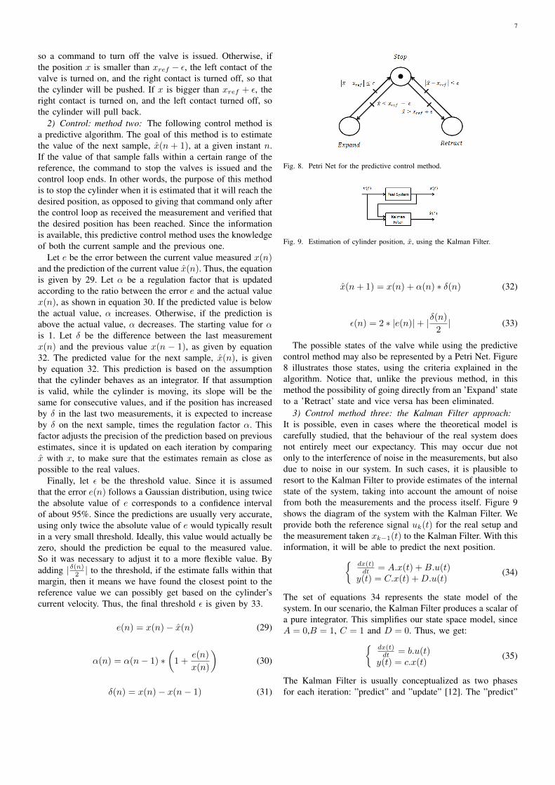
Fig. 8. Petri Net for the predictive control method.

Fig. 9. Estimation of cylinder position, x, using the Kalman Filter.

x(n+ 1) = x(n) + α(n) ∗ δ(n) (32)

ε(n) = 2 ∗ |e(n)|+ |δ(n)

2| (33)

The possible states of the valve while using the predictivecontrol method may also be represented by a Petri Net. Figure8 illustrates those states, using the criteria explained in thealgorithm. Notice that, unlike the previous method, in thismethod the possibility of going directly from an ’Expand’ stateto a ’Retract’ state and vice versa has been eliminated.

3) Control method three: the Kalman Filter approach:It is possible, even in cases where the theoretical model iscarefully studied, that the behaviour of the real system doesnot entirely meet our expectancy. This may occur due notonly to the interference of noise in the measurements, but alsodue to noise in our system. In such cases, it is plausible toresort to the Kalman Filter to provide estimates of the internalstate of the system, taking into account the amount of noisefrom both the measurements and the process itself. Figure 9shows the diagram of the system with the Kalman Filter. Weprovide both the reference signal uk(t) for the real setup andthe measurement taken xk−1(t) to the Kalman Filter. With thisinformation, it will be able to predict the next position.

dx(t)dt = A.x(t) +B.u(t)

y(t) = C.x(t) +D.u(t)(34)

The set of equations 34 represents the state model of thesystem. In our scenario, the Kalman Filter produces a scalar ofa pure integrator. This simplifies our state space model, sinceA = 0,B = 1, C = 1 and D = 0. Thus, we get:

dx(t)dt = b.u(t)

y(t) = c.x(t)(35)

The Kalman Filter is usually conceptualized as two phasesfor each iteration: ”predict” and ”update” [12]. The ”predict”

8

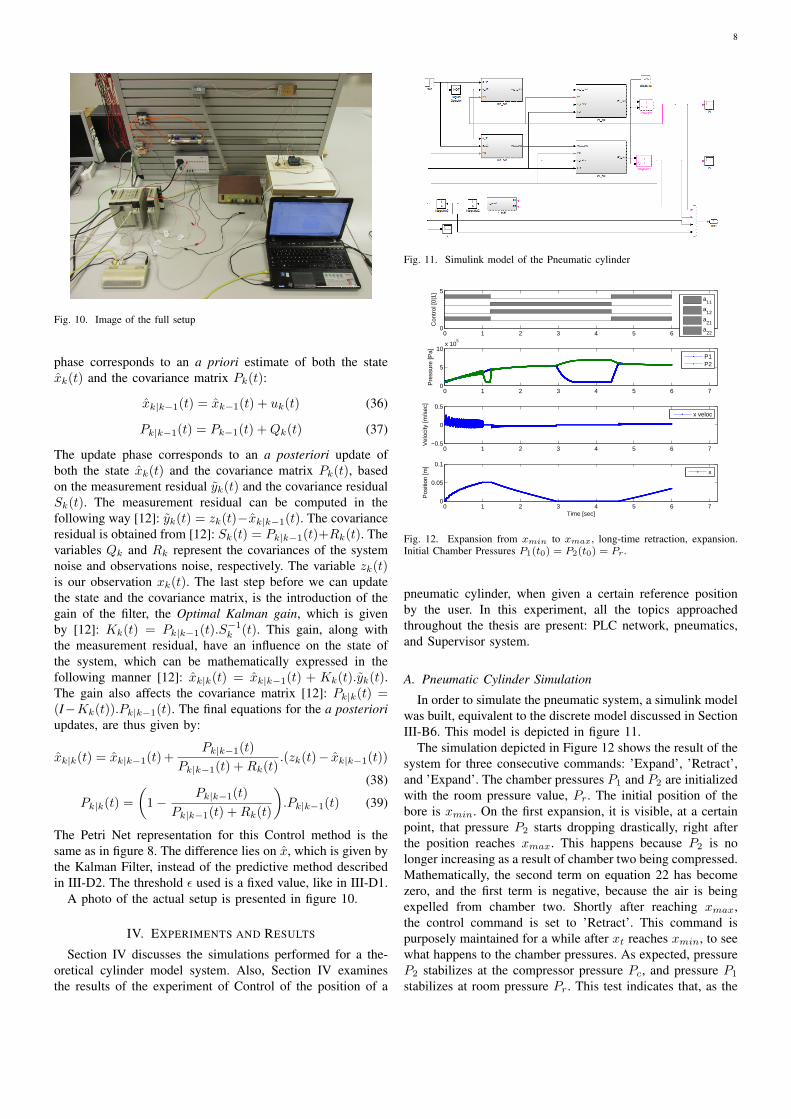
Fig. 10. Image of the full setup

phase corresponds to an a priori estimate of both the statexk(t) and the covariance matrix Pk(t):

xk|k−1(t) = xk−1(t) + uk(t) (36)

Pk|k−1(t) = Pk−1(t) +Qk(t) (37)

The update phase corresponds to an a posteriori update ofboth the state xk(t) and the covariance matrix Pk(t), basedon the measurement residual yk(t) and the covariance residualSk(t). The measurement residual can be computed in thefollowing way [12]: yk(t) = zk(t)−xk|k−1(t). The covarianceresidual is obtained from [12]: Sk(t) = Pk|k−1(t)+Rk(t). Thevariables Qk and Rk represent the covariances of the systemnoise and observations noise, respectively. The variable zk(t)is our observation xk(t). The last step before we can updatethe state and the covariance matrix, is the introduction of thegain of the filter, the Optimal Kalman gain, which is givenby [12]: Kk(t) = Pk|k−1(t).S−1k (t). This gain, along withthe measurement residual, have an influence on the state ofthe system, which can be mathematically expressed in thefollowing manner [12]: xk|k(t) = xk|k−1(t) + Kk(t).yk(t).The gain also affects the covariance matrix [12]: Pk|k(t) =(I−Kk(t)).Pk|k−1(t). The final equations for the a posterioriupdates, are thus given by:

xk|k(t) = xk|k−1(t) +Pk|k−1(t)

Pk|k−1(t) +Rk(t).(zk(t)− xk|k−1(t))

(38)

Pk|k(t) =

(1−

Pk|k−1(t)

Pk|k−1(t) +Rk(t)

).Pk|k−1(t) (39)

The Petri Net representation for this Control method is thesame as in figure 8. The difference lies on x, which is given bythe Kalman Filter, instead of the predictive method describedin III-D2. The threshold ε used is a fixed value, like in III-D1.

A photo of the actual setup is presented in figure 10.

IV. EXPERIMENTS AND RESULTS

Section IV discusses the simulations performed for a the-oretical cylinder model system. Also, Section IV examinesthe results of the experiment of Control of the position of a

Fig. 11. Simulink model of the Pneumatic cylinder

0 1 2 3 4 5 6 70

5

Con

trol

[0|1

]

a

11

a12

a21

a22

0 1 2 3 4 5 6 70

5

10x 10

5

Pre

ssur

e [P

a]

P1P2

0 1 2 3 4 5 6 70

0.05

0.1

Time [sec]

Pos

ition

[m]

x

0 1 2 3 4 5 6 7−0.5

0

0.5

Vel

ocity

[m/s

ec]

x veloc

Fig. 12. Expansion from xmin to xmax, long-time retraction, expansion.Initial Chamber Pressures P1(t0) = P2(t0) = Pr .

pneumatic cylinder, when given a certain reference positionby the user. In this experiment, all the topics approachedthroughout the thesis are present: PLC network, pneumatics,and Supervisor system.

A. Pneumatic Cylinder Simulation

In order to simulate the pneumatic system, a simulink modelwas built, equivalent to the discrete model discussed in SectionIII-B6. This model is depicted in figure 11.

The simulation depicted in Figure 12 shows the result of thesystem for three consecutive commands: ’Expand’, ’Retract’,and ’Expand’. The chamber pressures P1 and P2 are initializedwith the room pressure value, Pr. The initial position of thebore is xmin. On the first expansion, it is visible, at a certainpoint, that pressure P2 starts dropping drastically, right afterthe position reaches xmax. This happens because P2 is nolonger increasing as a result of chamber two being compressed.Mathematically, the second term on equation 22 has becomezero, and the first term is negative, because the air is beingexpelled from chamber two. Shortly after reaching xmax,the control command is set to ’Retract’. This command ispurposely maintained for a while after xt reaches xmin, to seewhat happens to the chamber pressures. As expected, pressureP2 stabilizes at the compressor pressure Pc, and pressure P1

stabilizes at room pressure Pr. This test indicates that, as the

9

(a) Simulink representation, considering constant gain K.

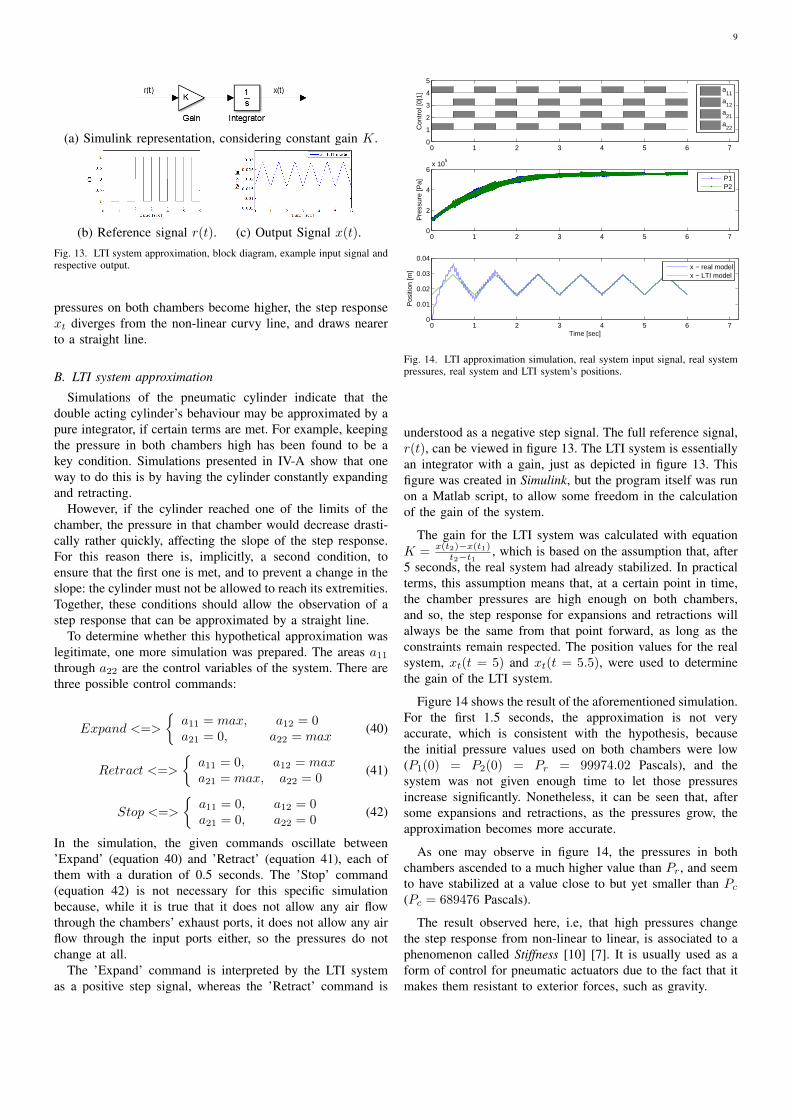
(b) Reference signal r(t). (c) Output Signal x(t).Fig. 13. LTI system approximation, block diagram, example input signal andrespective output.

pressures on both chambers become higher, the step responsext diverges from the non-linear curvy line, and draws nearerto a straight line.

B. LTI system approximation

Simulations of the pneumatic cylinder indicate that thedouble acting cylinder’s behaviour may be approximated by apure integrator, if certain terms are met. For example, keepingthe pressure in both chambers high has been found to be akey condition. Simulations presented in IV-A show that oneway to do this is by having the cylinder constantly expandingand retracting.

However, if the cylinder reached one of the limits of thechamber, the pressure in that chamber would decrease drasti-cally rather quickly, affecting the slope of the step response.For this reason there is, implicitly, a second condition, toensure that the first one is met, and to prevent a change in theslope: the cylinder must not be allowed to reach its extremities.Together, these conditions should allow the observation of astep response that can be approximated by a straight line.

To determine whether this hypothetical approximation waslegitimate, one more simulation was prepared. The areas a11through a22 are the control variables of the system. There arethree possible control commands:

Expand <=>

a11 = max, a12 = 0a21 = 0, a22 = max

(40)

Retract <=>

a11 = 0, a12 = maxa21 = max, a22 = 0

(41)

Stop <=>

a11 = 0, a12 = 0a21 = 0, a22 = 0

(42)

In the simulation, the given commands oscillate between’Expand’ (equation 40) and ’Retract’ (equation 41), each ofthem with a duration of 0.5 seconds. The ’Stop’ command(equation 42) is not necessary for this specific simulationbecause, while it is true that it does not allow any air flowthrough the chambers’ exhaust ports, it does not allow any airflow through the input ports either, so the pressures do notchange at all.

The ’Expand’ command is interpreted by the LTI systemas a positive step signal, whereas the ’Retract’ command is

0 1 2 3 4 5 6 70

1

2

3

4

5

Con

trol

[0|1

]

a

11

a12

a21

a22

0 1 2 3 4 5 6 70

2

4

6x 10

5

Pre

ssur

e [P

a]

P1P2

0 1 2 3 4 5 6 70

0.01

0.02

0.03

0.04

Time [sec]

Pos

ition

[m]

x − real modelx − LTI model

Fig. 14. LTI approximation simulation, real system input signal, real systempressures, real system and LTI system’s positions.

understood as a negative step signal. The full reference signal,r(t), can be viewed in figure 13. The LTI system is essentiallyan integrator with a gain, just as depicted in figure 13. Thisfigure was created in Simulink, but the program itself was runon a Matlab script, to allow some freedom in the calculationof the gain of the system.

The gain for the LTI system was calculated with equationK = x(t2)−x(t1)

t2−t1 , which is based on the assumption that, after5 seconds, the real system had already stabilized. In practicalterms, this assumption means that, at a certain point in time,the chamber pressures are high enough on both chambers,and so, the step response for expansions and retractions willalways be the same from that point forward, as long as theconstraints remain respected. The position values for the realsystem, xt(t = 5) and xt(t = 5.5), were used to determinethe gain of the LTI system.

Figure 14 shows the result of the aforementioned simulation.For the first 1.5 seconds, the approximation is not veryaccurate, which is consistent with the hypothesis, becausethe initial pressure values used on both chambers were low(P1(0) = P2(0) = Pr = 99974.02 Pascals), and thesystem was not given enough time to let those pressuresincrease significantly. Nonetheless, it can be seen that, aftersome expansions and retractions, as the pressures grow, theapproximation becomes more accurate.

As one may observe in figure 14, the pressures in bothchambers ascended to a much higher value than Pr, and seemto have stabilized at a value close to but yet smaller than Pc(Pc = 689476 Pascals).

The result observed here, i.e, that high pressures changethe step response from non-linear to linear, is associated to aphenomenon called Stiffness [10] [7]. It is usually used as aform of control for pneumatic actuators due to the fact that itmakes them resistant to exterior forces, such as gravity.

10

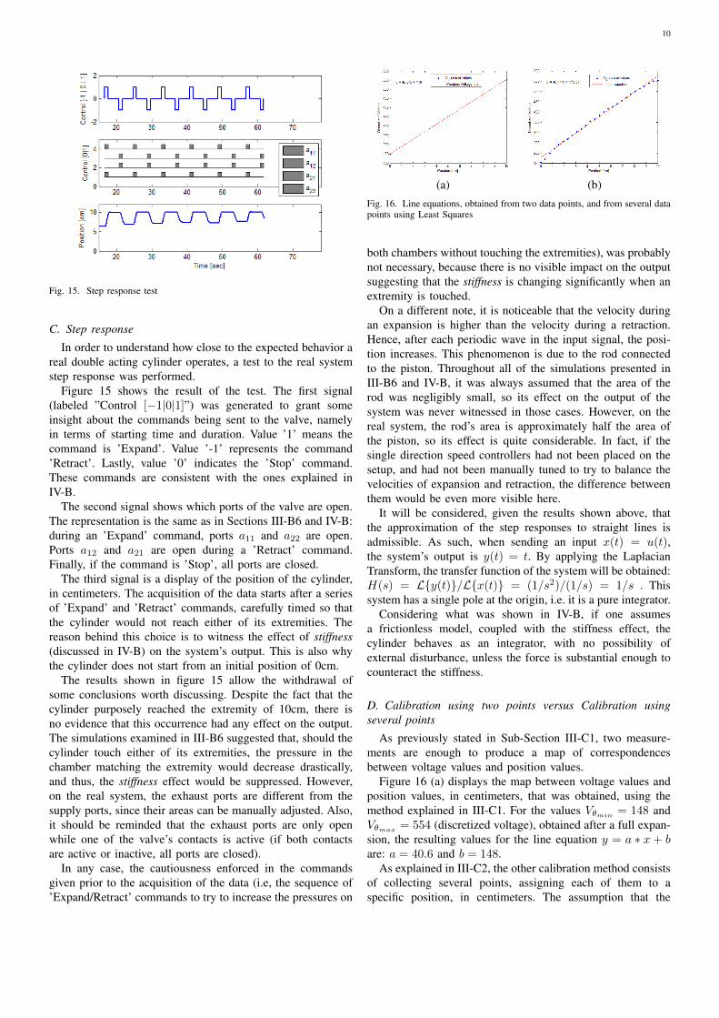
Fig. 15. Step response test

C. Step response

In order to understand how close to the expected behavior areal double acting cylinder operates, a test to the real systemstep response was performed.

Figure 15 shows the result of the test. The first signal(labeled ”Control [−1|0|1]”) was generated to grant someinsight about the commands being sent to the valve, namelyin terms of starting time and duration. Value ’1’ means thecommand is ’Expand’. Value ’-1’ represents the command’Retract’. Lastly, value ’0’ indicates the ’Stop’ command.These commands are consistent with the ones explained inIV-B.

The second signal shows which ports of the valve are open.The representation is the same as in Sections III-B6 and IV-B:during an ’Expand’ command, ports a11 and a22 are open.Ports a12 and a21 are open during a ’Retract’ command.Finally, if the command is ’Stop’, all ports are closed.

The third signal is a display of the position of the cylinder,in centimeters. The acquisition of the data starts after a seriesof ’Expand’ and ’Retract’ commands, carefully timed so thatthe cylinder would not reach either of its extremities. Thereason behind this choice is to witness the effect of stiffness(discussed in IV-B) on the system’s output. This is also whythe cylinder does not start from an initial position of 0cm.

The results shown in figure 15 allow the withdrawal ofsome conclusions worth discussing. Despite the fact that thecylinder purposely reached the extremity of 10cm, there isno evidence that this occurrence had any effect on the output.The simulations examined in III-B6 suggested that, should thecylinder touch either of its extremities, the pressure in thechamber matching the extremity would decrease drastically,and thus, the stiffness effect would be suppressed. However,on the real system, the exhaust ports are different from thesupply ports, since their areas can be manually adjusted. Also,it should be reminded that the exhaust ports are only openwhile one of the valve’s contacts is active (if both contactsare active or inactive, all ports are closed).

In any case, the cautiousness enforced in the commandsgiven prior to the acquisition of the data (i.e, the sequence of’Expand/Retract’ commands to try to increase the pressures on

(a) (b)Fig. 16. Line equations, obtained from two data points, and from several datapoints using Least Squares

both chambers without touching the extremities), was probablynot necessary, because there is no visible impact on the outputsuggesting that the stiffness is changing significantly when anextremity is touched.

On a different note, it is noticeable that the velocity duringan expansion is higher than the velocity during a retraction.Hence, after each periodic wave in the input signal, the posi-tion increases. This phenomenon is due to the rod connectedto the piston. Throughout all of the simulations presented inIII-B6 and IV-B, it was always assumed that the area of therod was negligibly small, so its effect on the output of thesystem was never witnessed in those cases. However, on thereal system, the rod’s area is approximately half the area ofthe piston, so its effect is quite considerable. In fact, if thesingle direction speed controllers had not been placed on thesetup, and had not been manually tuned to try to balance thevelocities of expansion and retraction, the difference betweenthem would be even more visible here.

It will be considered, given the results shown above, thatthe approximation of the step responses to straight lines isadmissible. As such, when sending an input x(t) = u(t),the system’s output is y(t) = t. By applying the LaplacianTransform, the transfer function of the system will be obtained:H(s) = Ly(t)/Lx(t) = (1/s2)/(1/s) = 1/s . Thissystem has a single pole at the origin, i.e. it is a pure integrator.

Considering what was shown in IV-B, if one assumesa frictionless model, coupled with the stiffness effect, thecylinder behaves as an integrator, with no possibility ofexternal disturbance, unless the force is substantial enough tocounteract the stiffness.

D. Calibration using two points versus Calibration usingseveral points

As previously stated in Sub-Section III-C1, two measure-ments are enough to produce a map of correspondencesbetween voltage values and position values.

Figure 16 (a) displays the map between voltage values andposition values, in centimeters, that was obtained, using themethod explained in III-C1. For the values Vθmin = 148 andVθmax

= 554 (discretized voltage), obtained after a full expan-sion, the resulting values for the line equation y = a ∗ x + bare: a = 40.6 and b = 148.

As explained in III-C2, the other calibration method consistsof collecting several points, assigning each of them to aspecific position, in centimeters. The assumption that the

11

(a)

(b)

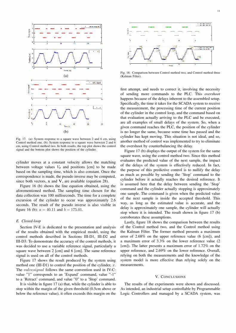
Fig. 17. (a): System response to a square wave between 2 and 6 cm, usingControl method one. (b): System response to a square wave between 2 and 6cm, using Control method two. In both results, the top plot shows the controlsignal and the bottom plot shows the position of the cylinder.

cylinder moves at a constant velocity allows the matchingbetween voltage values Vθ and positions [cm] to be madebased on the sampling time, which is also constant. Once thecorrespondence is made, the pseudo inverse may be computed,since both vectors, x and V, are available (equation 28).

Figure 16 (b) shows the line equation obtained, using theaforementioned method. The sampling time chosen for thedata collection was 100 milliseconds. The time for a completeexcursion of the cylinder to occur was approximately 2.6seconds. The result of the pseudo inverse is also visible infigure 16 (b): a = 40.11 and b = 175.01.

E. Closed-loop

Section IV-E is dedicated to the presentation and analysisof the results obtained with the empirical model, using thecontrol methods described in Sections III-D1, III-D2 andIII-D3. To demonstrate the accuracy of the control methods, itwas decided to use a variable reference signal, particularly asquare wave between 2 [cm] and 6 [cm]. The same referencesignal is used on all of the control methods.

Figure 17 shows the result produced by the system usingmethod one (III-D1) to control the position of the cylinder, x.The valvesignal follows the same convention used in IV-C:value ”1” corresponds to an ’Expand’ command, value ”-1”to a ’Retract’ command, and value ”0” to a ’Stop’ command.

It is visible in figure 17 (a) that, while the cylinder is able tostop within the margin of the given threshold (0.5cm above orbelow the reference value), it often exceeds this margin on the

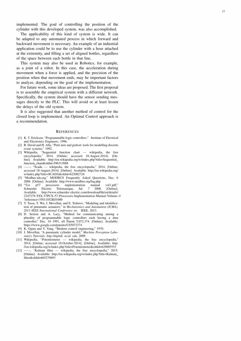
Fig. 18. Comparison between Control method two, and Control method three(Kalman Filter).

first attempt, and needs to correct it, involving the necessityof sending more commands to the PLC. This overshoothappens because of the delays inherent to the assembled setup.Specifically, the time it takes for the SCADA system to receivethe measurement, the processing time of the current positionof the cylinder in the control loop, and the command based onthat evaluation actually arriving to the PLC and be executed,are all examples of small delays of the system. So, when agiven command reaches the PLC, the position of the cylinderis no longer the same, because some time has passed and thecylinder has kept moving. This situation is not ideal, and so,another method of control was implemented to try to eliminatethe overshoot by counterbalancing the delay.

Figure 17 (b) displays the output of the system for the samesquare wave, using the control method two. Since this methodevaluates the predicted value of the next sample, the impactof the delays of the system is effectively reduced. In fact,the purpose of this predictive control is to nullify the delayas much as possible by sending the ’Stop’ command to thecylinder before it actually reaches the desired reference. Itis assumed here that the delay between sending the ’Stop’command and the cylinder actually stopping is approximatelyone sample. The command is given when the predicted valueof the next sample is inside the accepted threshold. Thisway, as long as the estimated value is accurate, and thedelay is approximately one sample, the cylinder will actuallystop where it is intended. The result shown in figure 17 (b)corroborates these assumptions.

Lastly, figure 18 shows the comparison between the resultsof the Control method two, and the Control method usingthe Kalman Filter. The former method presents a maximumerror of 2.68% on the upper reference value (6 [cm]), anda maximum error of 3.3% on the lower reference value (2[cm]). The latter presents a maximum error of 1.72% on theupper reference, and 2.69% on the lower reference. Overall,relying on both the measurements and the knowledge of thesystem model is more effective than relying solely on themeasurements.

V. CONCLUSIONS

The results of the experiments were shown and discussed.As intended, an industrial setup controllable by ProgrammableLogic Controllers and managed by a SCADA system, was

12

implemented. The goal of controlling the position of thecylinder with this developed system, was also accomplished.

The applicability of this kind of system is wide. It canbe adapted to any automated process in which forward andbackward movement is necessary. An example of an industrialapplication could be to use the cylinder with a hose attachedat the extremity, and filling a set of aligned bottles, regardlessof the space between each bottle in that line.

This system may also be used in Robotics, for example,as a joint of a robot. In this case, the acceleration duringmovement when a force is applied, and the precision of theposition when that movement ends, may be important factorsto analyze, depending on the goal of the implementation.

For future work, some ideas are proposed. The first proposalis to assemble the empirical system with a different network.Specifically, the system should have the sensor sending mes-sages directly to the PLC. This will avoid or at least lessenthe delays of the old system.

It is also suggested that another method of control for theclosed loop is implemented. An Optimal Control approach isa recommendation.

REFERENCES

[1] K. T. Erickson, “Programmable logic controllers.” Institute of Electricaland Electronics Engineers, 1996.

[2] R. David and H. Alla, “Petri nets and grafcet: tools for modelling discreteevent systems,” 1992.

[3] Wikipedia, “Sequential function chart — wikipedia, the freeencyclopedia,” 2014, [Online; accessed 18-August-2014]. [On-line]. Available: http://en.wikipedia.org/w/index.php?title=Sequentialfunction chart&oldid=596313068

[4] ——, “Scada — wikipedia, the free encyclopedia,” 2014, [Online;accessed 18-August-2014]. [Online]. Available: http://en.wikipedia.org/w/index.php?title=SCADA&oldid=622082724

[5] “Modbus-ida.org,” MODBUS Frequently Asked Questions, Dec. 62006. [Online]. Available: http://www.modbus.org/faq.php

[6] “Tsx p57 processors implementation manual vol1.pdf,”Schneider Electric Telemanique, Jul. 7 2008. [Online].Available: http://www.schneider-electric.com/download/hk/en/details/2247279-TSX-57PCX-57-Processors-Implementation-Manual-Volume-1/?reference=35011052K01000

[7] Y. Tassa, T. Wu, J. Movellan, and E. Todorov, “Modeling and identifica-tion of pneumatic actuators,” in Mechatronics and Automation (ICMA),2013 IEEE International Conference on. IEEE, 2013.

[8] D. Sexton and A. Lacy, “Method for communicating among aplurality of programmable logic controllers each having a dmacontroller,” Dec. 10 1991, uS Patent 5,072,374. [Online]. Available:https://www.google.com/patents/US5072374

[9] K. Ogata and Y. Yang, “Modern control engineering,” 1970.[10] J. Movellan, “A pneumatic cylinder model,” Machine Perception Labo-

ratory Tutorials, http://mplab. ucsd. edu, 2009.[11] Wikipedia, “Potentiometer — wikipedia, the free encyclopedia,”

2014, [Online; accessed 10-October-2014]. [Online]. Available: http://en.wikipedia.org/w/index.php?title=Potentiometer&oldid=629005553

[12] ——, “Kalman filter — wikipedia, the free encyclopedia,” 2015.[Online]. Available: http://en.wikipedia.org/w/index.php?title=Kalmanfilter&oldid=665279693