NASA/TMB1998-206316

Neural Network and Regression

Approximations in High Speed Civil

Transport Aircraft Design Optimization

Surya N. Patnaik

Ohio Aerospace Institute, Cleveland, Ohio

James D. Guptill, Dale A. Hopkins, and Thomas M. Lavelle

Lewis Research Center, Cleveland, Ohio

National Aeronautics and

Space Administration

Lewis Research Center

April 1998

https://ntrs.nasa.gov/search.jsp?R=19980151078 2018-07-06T18:57:09+00:00Z

Trade names or manufacturers' names are used in this report for

identification onl3a This usage does not constitute an official

endorsement, either expressed or implied, by the National

Aeronautics and Space Administration.

NASA Center for Aerospace Information

800 Elkridge Landing Road

Linthicum Heights, MD 21090-2934Price Code: A03

Available from

National Technical Information Service

5287 Port Royal Road

Springfield, VA 22100Price Code: A03

NEURAL NETWORK AND REGRESSION APPROXIMATIONS IN HIGH

SPEED CIVIL TRANSPORT AIRCRAFT DESIGN OPTIMIZATION

Surya N. Patnaik*

Ohio Aerospace Institute, Brook Park, Ohio

James D. Guptill t, Dale A. Hopkins', and Thomas M. Lavelle§

National Aeronautics and Space AdminstationLewis Research Center

Cleveland, Ohio 44135

SUMMARY

Nonlinear mathematical-programming-based design optimization can be an elegant method. However, the cal-

culations required to generate the merit function, constraints, and their gradients, which are frequently required,

can make the process computationally intensive. The computational burden can be greatly reduced by using approxi-

mating analyzers derived from an original analyzer utilizing neural networks and linear regression methods. The

experience gained from using both of these approximation methods in the design optimization of a high speed civil

transport aircraft is the subject of this paper. The Langley Research Center's Flight Optimization System was

selected for the aircraft analysis. This software was exercised to generate a set of training data with which a neural

network and a regression method were trained, thereby producing the two approximating analyzers. The derived

analyzers were coupled to the Lewis Research Center's CometBoards test bed to provide the optimization capability.

With the combined software, both approximation methods were examined for use in aircraft design optimization,

and both performed satisfactorily. The CPU time for solution of the problem, which had been measured in hours,

was reduced to minutes with the neural network approximation and to seconds with the regression method. Instabil-

ity encountered in the aircraft analysis software at certain design points was also eliminated. On the other hand,

there were costs and difficulties associated with training the approximating analyzers. The CPU time required to

generate the input-output pairs and to train the approximating analyzers was seven times that required for solution of

the problem.

INTRODUCTION

Intensive computation can be a serious deficiency in an otherwise elegant nonlinear mathematical-

programming-based design optimization method. In typical structural design applications, most of the computations,

often more than 99 percent of the total calculations, can be traced to the analyzer (ref. 1). That is, reanalysis and

sensitivity calculations consume the bulk of the computation time in design optimization. To reduce the computa-

tional burden, two approximation methods, regression analysis and neural networks, have been incorporated into theNASA Lewis Research Center's design test bed CometBoards (refs. 1 to 3) (Comparative Evaluation Test Bed of

Optimization and Analysis Routines for the Design of Structures). Both approximation methods provide the reanaly-

sis and design sensitivity information that is usually required during optimization. Approximation augmentation,

which includes a strategy to select training pairs, has broadened the scope of CometBoards; thus, a design problem

can be solved by using three different analyzers the original analyzer or one of the two derived analyzers that are

based on regression and neural networks.

The example of a high speed civil transport (HSCT) aircraft is considered to examine the performance of

approximation methods in design optimization. The NASA Langley Research Center's Flight Optimization System,

FLOPS (refs. 4 and 5), which is well known in industry, was chosen as the aircraft analyzer. This analyzer is not just

*Engineer, Associate Fellow AIAA.

tMathematician, Computational Sciences Branch.

_;Acting Chief, Structural Mechanics Branch, Senior Member AIAA.

§Engineer, Propulsion System Analysis Office.

No copyright is asserted in the United States.

NASA/TM-- 1998-206316 1

computationallyintensive; it can also become unstable at certain design points, thereby requiring that the optimiza-

tion process be restarted. Moreover, an optimum benchmark solution established for the HSCT aircraft problem

from results generated previously with the FLOPS analyzer by Langley, Lewis, and industry becomes a useful solu-

tion against which the results obtained with the approximation methods can be compared. CometBoards, which in-

cludes an approximation module containing regression analysis as well as neural networks, has been soft-coupled to

the FLOPS analyzer. The CometBoards-FLOPS combined software can optimize an HSCT aircraft by using any one

of the three analyzers--the original FLOPS code, the derived regression, or neural network models. This paper pre-

sents optimal solutions that were generated for the HSCT aircraft by using all three analyzers. The results are exam-

ined to assess the performance of the approximation methods in the design of an HSCT aircraft system. In specific

terms, the deviation in the aircraft weight and behavior constraints, and their sensitivity, are investigated for analysis

as well as design. The computational efficiency achieved by using approximation methods in design optimization is

examined by comparing CPU solution times.

This paper is organized as follows: an overview of the CometBoards design test bed; a brief description of

the aircraft analyzer FLOPS; a strategy to generate the input portion of the input-output (io) pairs for training both

approximating analyzers; a brief description of regression analysis and neural networks; a definition of the design

problem and the benchmark solution; generation of the io pairs for this problem; representative response prediction

through the approximation methods; the performance of both approximation methods in predicting the behavior

parameters of the aircraft; their performance during design optimization; and conclusions.

COMETBOARDS: A DESIGN TEST BED

Our earlier research to compare different optimization algorithms and alternate analysis methods for structural

design applications has grown into a multidisciplinary design test bed that is still referred to by its original acronym,

CometBoards. The modular organization of CometBoards (see fig. 1) allows innovative methods to be quickly vali-

dated through the integration of new programs into its existing modules. Optimizers and analyzers are two importantmodules of CometBoards. The optimizer module includes a number of algorithms, such as the fully utilized design

(ref. 6), optimality criteria methods (ref. 6), the method of feasible directions (ref. 7), the modified method of fea-sible directions (ref. 8), three different sequential quadratic programming techniques (refs. 9 to 11), the Sequential

Unconstrained Minimizations Technique (ref. 12), sequential linear programming (ref. 7), a reduced gradient

method (ref. 13), and others. Likewise, the analyzer module includes COSMIC/NASTRAN (ref. 14), the nonlinear

analyzer MHOST (ref. 15), the U.S. Air Force ANALYZE/DANALYZE (ref. 16), IFM/ANALYZERS (ref. 17), the

aircraft flight optimization analysis code FLOPS (ref. 5), the NASA Engine Performance Program NEPP (ref. 18),and others. Some of the other unique features of CometBoards include a cascade optimization strategy, design vari-

able and constraint formulations, a global scaling strategy, analysis and sensitivity approximations through regres-

sion and neural networks, and substructure optimization on sequential as well as parallel computational platforms

(ref. 19). CometBoards has provisions to accommodate up to l0 different disciplines, each of which can have a

maximum of 5 subproblems. The test bed can optimize a large system, which can be defined in as many as 50 differ-

ent subproblems. Alternatively, a component of a large system can be optimized in order to improve an existing

system. The design test bed has been successfully used to solve a number of problems, such as the structural design

of space station components; the design of nozzle components for air-breathing engines; and the configuration

design of subsonic and supersonic aircraft, mixed flow turbofan engines, and wave rotor concepts in engines.

CometBoards has over 50 numerical examples in its test bed. It is written in FORTRAN 77, except for the neural

network code, Cometnet (ref. 20), which is written in C++. The process of integrating this C++ code into the

CometBoards FORTRAN 77 code is referred to as soft-coupling. Soft-coupling is achieved by first generating anexecutable file from the Cometnet C++ source code; then Cometnet is invoked from CometBoards through a system

call. Information is exchanged between the two programs through data files. At present CometBoards is available on

UNIX-based Cray and Convex computers and on Iris and Sun workstations. CometBoards is continuously being

improved to increase its reliability and robustness for optimization at system as well as component levels. This paper

emphasizes the approximation module of CometBoards, which includes regression analysis and neural network ap-

proximations for the design optimization of an HSCT aircraft.

NASA/TM--1998-206316 2

FLOPS:ANAIRCRAFTANALYZER

Aircraftdesignwasformulatedasanonlinearprogrammingproblemwithasetofdesignvariablestooptimizeameritfunctionunderasetofbehaviorconstraints.TheFLOPSanalyzerevaluatedtheperformanceparametersofanadvancedaircrafttogeneratetheconstraintsandmeritfunction.Bysoft-couplingLewis'CometBoardsandLangley'sFLOPS,thedesignproblemcouldbesetupandsolvedwithoutmajormodificationtoeithercode.ThedesignproblemwassolvedbyusingtheCometBoards-FLOPScombinedcapability.

TheFLOPSanalyzerhaseightdisciplines:weightestimation,aerodynamicanalysis(refs.21and22),enginecycleanalysis(refs.23to25),propulsiondatainterpolation,missionperformance,airfieldlengthrequirementsfortakeoffandlanding,noisefootprintcalculations(ref.26),andcostestimation(refs.27to32).TheFLOPSanalyzerallowsselectionofthefollowingfreevariablesforthepurposeofoptimization:(1)rampweight,(2)wingaspectratio,(3)enginethrust,(4)taperratioofthewing,(5)referencewingarea,(6)quarterchordsweepangleofthewing,(7)wingthicknesstochordratio,(8)cruiseMachnumber,(9)cruisealtitude,(10)enginedesignpointturbineentrytemperature,(11)overallpressureratio,(12)bypassratioforturbofanengines,(13)fanpressureratioforturbofanengines,and(14)enginethrottleratio(definedastheratioofmaximumallowableturbineinlettemperaturedividedbythedesignpointturbineinlettemperature).FortheHSCTproblem,thefreevariableswereseparatedintoasetofsixactivedesignvariablesandasetofeightpassivedesignvariables.

Forthepurposeofoptimization,thecompositemeritfunctionavailableinFLOPScanbewrittenas

7Obj = ___ Wk#k

k=l

(1)

where Obj represents the merit function, wk represents the kth weight factor, and the parameter flk can be selectedfrom the following list: (1) gross takeoff weight of the aircraft, (2) mission fuel, (3) the product of the Mach number

times the ratio of lift-to-drag, (4) range, (5) cost, (6) specific fuel consumption, and (7) NOx emissions. For the

HSCT problem, the gross takeoff weight was selected as the merit function by setting w I =1.0 and the other weightfactors to zero.

Behavior constraints can be imposed on (1) the missed approach climb gradient thrust, (2) the second-segment

climb thrust, (3) the landing approach velocity, (4) the takeoff field length, (5) the jet velocity, (6) the compressor

discharge temperature, (7) the total usable fuel weight, (8) the range of the flight, (9) the landing field length,

(10) the aspect ratio (defined as the ratio of bypass area to the core area of a mixed flow turbofan engine), (11) the

engine-throttle ratio, (12) the specific fuel consumption, (13) the compressor discharge pressure, (14) the excess

fuel, and others. Only the first six constraints were imposed in the HSCT problem.

The design space of an aircraft optimization problem can be distorted because both design variables and con-straints vary over a wide range. For example, an engine thrust design variable (which is measured in kilopounds,

e.g., 40 000 lb) is immensely different from the bypass ratio variable (which is a small number, e.g., 0.5). Likewise,

a landing velocity constraint in knots and a field length limitation in thousands of feet differ both in magnitude and

in units of measure. In CometBoards the distortion is reduced by scaling the merit function, design variables, and

constraints such that their normalized values are around unity.

SELECTION STRATEGY FOR INPUT PORTION OF INPUT-OUTPUT PAIRS FOR TRAINING

Both regression and neural network approximations require a set of io pairs for their training. Since intrinsic

coupling of design variables can be inherent to large design problems, this coupling can be exploited to increase the

efficiency of the training scheme. A strategy has been devised to generate a set of design variables that forms the

input portion of the training pairs for a specified coupling map. The output portion, representing the merit function

and behavior constraints, is generated from the FLOPS analyzer for the specified input design variables. An example

of a design problem with six active variables (1 to 5 and 7) and one passive variable (6) is used to illustrate the input

variable selection strategy. The six active variables are separated into four related sets, designated by circled digits 1

to 4 in figure 2. The design variables are shown in braces: {4,7}, {2}, {3,5}, and { 1,2,7} for sets 1 through 4, re-

spectively. Their coupling and influence regions, shown in figure. 2, are given in table I.

NASA/TM--1998-206316 3

In table I consider, for example, Set 3 with two influence regions (2 and 4, see fig. 2). Response prediction for

Set 3 (with two active design variables of its own) will include those of its coupling regions (design variables 1, 2, 3,5, and 7). These five variables will be perturbed by using the scheme described next, and in addition, other active

variables may also undergo minor perturbations.

Consider a design variable in a set with initial design Zi, upper bound Z u, and lower bound XI. Divide the inter-

val between the lower bound and the initial design, and that between the initial design and the upper bound, into nil

and niu subintervals, respectively. A bandwidth bw is assigned for the design variable that specifies the number ofsubintervals to be grouped together to form random perturbations. To illustrate the strategy for selecting the input

portion of a set of io pairs, let us consider a simple example with two design variables. The perturbation scheme

requires the following data for each design variable:

(1) Design variable 1: lower, initial, and upper bounds of, for example, 0.05, 4.00, and 10.00, respectively.

(2) Design variable 2: lower, initial, and upper bounds of, for example, 0.50, 6.00, and 9.50, respectively.

Let us divide the intervals between the lower bound and the initial design into four subintervals. Likewise,

divide the interval between the initial design and the upper bound into three subintervals. Assume a bandwidth of

bw = 3. Further, specify the number of perturbations for each subinterval as follows: for the four subintervals begin-

ning from the initial design toward the lower bound--15, 10, 2, and 6; and for the three subintervals from the initial

design to the upper bound--10, 4, and 8.

The input portion of the io pairs generated through the selection strategy is depicted in figure 3. There are 131

design points. The inner circle, with a radius of 2 centered on the initial design (4,6), captures 31 design points,which corresponds to a density of 2.5 points per unit area. The annulus with radii of 2 and 3 also contains 31 design

points, but is less dense with 2.0 points per unit area. A satisfactory pattern for the input portion of the io pairs can

be generated by changing the bandwidth, number of intervals, stations, and perturbations in an iterative fashion.

Linear Regression Analysis

Regression analysis available in CometBoards uses several basis functions. The basis functions can be selected

from (1) a full cubic polynomial, (2) a quadratic polynomial, (3) a linear polynomial in reciprocal variables, (4) a

quadratic polynomial in reciprocal variables, and (5) combinations thereof. Consider, for example, regression analy-

sis of an n variable model with a combination of a cubic polynomial in design variables and a quadratic polynomial

in reciprocal design variables. The regression function has the following explicit form:

n n /I n /1 n /,1 /I n

y(_)= flO + 2flixi +EEflijxixj +2E 2flijkXiXjXk + 2_i l_._+E Eflij- xixjli=1 i=1 j=i i=1 j=ik=j i=1 _ i=1 j=i

(2)

The regression coefficients ]_ are determined by using the linear least squares approach incorporated in the DGELS

(double precision general matrix linear least squares solver) routine of the Lapack library (ref. 33). The gradient

matrix of the regression function with respect to the design variables is obtained in closed form. For the example

with n variables, the gradient matrix for the regression function has the following form:

"0

O_Xl

0

Vy =.0x 2

OnXn

y (3)

where

NASA/TM-- 1998-206316 4

OqXl i=l i=l j=i+l i=1 j=i "=

and fl(i= _jifori>j, _i)k= flikjforj> k > i,etc.Once theregressioncoefficientshave been obtainedfrom thesingletrainingcycle,reanalysisand sensitivity

calculationsrepresentedby equations(2)to(4)requiretrivialcomputationaleffort.Inregressionanalysis,the accu-

racyoftheapproximationfunctionand itsgradientcan differsignificantlynear,aswellasoutsideof,theboundary

ofthetrainingdomain.Thisdeficiency,ifany,inCometBoards can be reducedby selectingeitherclosed-formor

finitedifferencegradients,atthe discretionoftheuser.

NEURAL NETWORK APPROXIMATIONS

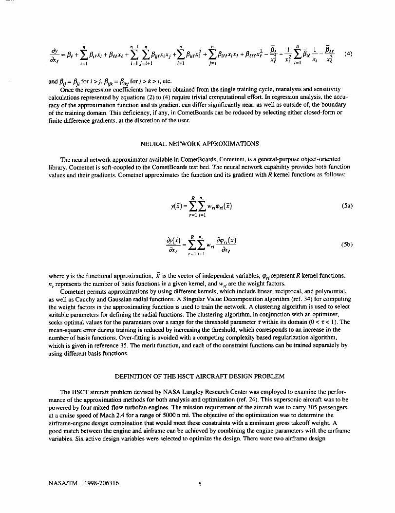
The neural network approximator available in CometBoards, Cometnet, is a general-purpose object-oriented

library. Cometnet is soft-coupled to the CometBoards test bed. The neural network capability provides both function

values and their gradients. Cometnet approximates the function and its gradient with R kernel functions as follows:

g tl r

Y(x ) : _._ E Wri_Ori('r)r=l i=l

(Sa)

R nr C_(Pri(.________)

dY( )-EEw" dx,OqX_ r=l i=1

(5b)

where y is the functional approximation, ._ is the vector of independent variables, tpr/ represent R kernel functions,

nr represents the number of basis functions in a given kernel, and Wr/are the weight factors.Cometnet permits approximations by using different kernels, which include linear, reciprocal, and polynomial,

as well as Cauchy and Gaussian radial functions. A Singular Value Decomposition algorithm (ref. 34) for computing

the weight factors in the approximating function is used to train the network. A clustering algorithm is used to selectsuitable parameters for defining the radial functions. The clustering algorithm, in conjunction with an optimizer,

seeks optimal values for the parameters over a range for the threshold parameter "rwithin its domain (0 < z < 1). The

mean-square error during training is reduced by increasing the threshold, which corresponds to an increase in the

number of basis functions. Over-fitting is avoided with a competing complexity based regularization algorithm,

which is given in reference 35. The merit function, and each of the constraint functions can be trained separately by

using different basis functions.

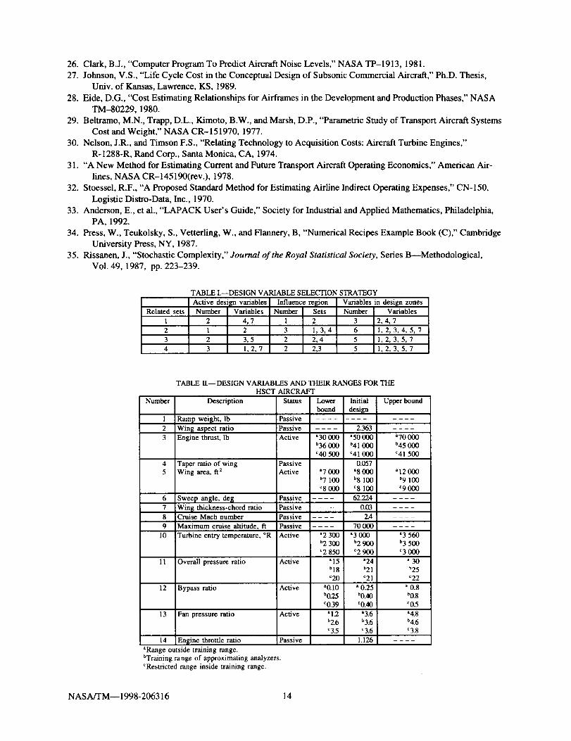
DEFINITION OF THE HSCT AIRCRAFT DESIGN PROBLEM

The HSCT aircraft problem devised by NASA Langley Research Center was employed to examine the perfor-

mance of the approximation methods for both analysis and optimization (ref. 24). This supersonic aircraft was to be

powered by four mixed-flow turbofan engines. The mission requirement of the aircraft was to carry 305 passengers

at a cruise speed of Mach 2.4 for a range of 5000 n mi. The objective of the optimization was to determine the

airframe-engine design combination that would meet these constraints with a minimum gross takeoff weight. A

good match between the engine and airframe can be achieved by combining the engine parameters with the airframe

variables. Six active design variables were selected to optimize the design. There were two airframe design

NASA/TM--1998-206316 5

variables--theenginethrustandthewingsize--andfourenginedesignparameters---theturbineinlettemperature,theoverallpressureratio,thebypassratio,andthefanpressureratio.Theturbineinlettemperaturewaslimitedtoamaximumof3560°R. The constraints imposed on the aircraft and engine were as follows: The takeoff and landing

field lengths had to be less than 11 000 ft; the approach velocity had to be less than 160 kn; there had to be enough

volume to carry all the required fuel; there had to be enough engine thrust available to recover from a missed ap-

proach and execute a second-segment climb; the exit jet velocity had to be less than 2300 ft/sec to limit engine

noise; and the compressor discharge temperature had to be less than 1710 °R.

To assess the performance of the approximation methods, the design space was divided into three subregions:

the standard, wide, and restricted ranges. The range used to train the approximating analyzers is referred to as the

standard range and designated with the letter "b" in table II. The wide range, designated by the letter "a," is

defined as the range outside the training range. The restricted range, designated by the letter "c," is defined as the

range inside the training range. The design variables, their ranges, and status (active or passive) are specified intable II.

The six behavior constraints, which are implicit functions of the design variables, were as follows:

(1) Missed approach climb thrust tc, which must be positive; it was normalized with respect to 106 Ib

tc <0gl = - 1--_

(2) Second-segment climb thrust ts, which must be positive; it was normalized with respect to 104 lb

_ ts

g2 --]-_T <0

(3) Landing approach velocity va, which must not exceed 160 kns

(4)

g3 = Va -1<0160

Takeoff field length _et, which must not exceed 11 000 ft

g4 = gt --1 <_011000

(5) Jet velocity vj, which must not exceed 2300 kn

g5 = vj -1<02300

(6) Compressor discharge temperature T, which must not exceed 1710 °R

Tg6 - 1<0

1710

The constraints extracted from the FLOPS analyzer output in the soft-coupling process were passed into the

CometBoards design test bed. The problem has several passive constraints, which were excluded from design opti-mization calculations.

NASA/TM-- 1998-206316 6

BENCHMARKSOLUTIONFORTHEHSCTAIRCRAFT

NASALangley(reL23)posedsix test cases with different starting points and variable bounds for the HSCT

aircraft problem. NASA Lewis, using the CometBoards test bed and the FLOPS analyzer, obtained solutions for five

of these cases, as did an industrial partner using its own optimizer and the FLOPS analyzer. Table OI gives the opti-

mum weights of the aircraft under the five different conditions, as obtained by Lewis and the industrial partner.Case five is considered the benchmark solution against which all results, including neural network and regres-

sion answers, were compared. For the five cases given in table III, the gross takeoff weight of the HSCT aircraft

obtained by the two groups agreed within a maximum deviation of 1.79 percent. Overall, these results can be consid-

ered acceptable, with minor deviations, because aircraft optimization is a difficult problem. The problem may be

difficult because of the variation in the constraints over a wide range and because of the empirical equations and

smoothing techniques used in the FLOPS code. The weight, design variables, and constraints for the optimal solu-

tion of the benchmark case are given in table IV.

The optimum solutions (see table IV) were in agreement, with minor deviations, except for the second-segment

climb thrust. However, both values of this constraint, which must be positive, are acceptable. The number of re-

analyses required for the CometBoards and industry solutions (134 and 1240, respectively) differed because industryused a combination of a gradient-based algorithm along with a genetic code, which, for this problem, was comput-

ationally intensive. The optimum solution has also been verified graphically. At optimum there are three active con-

straints: takeoff field length, jet velocity, and compressor discharge temperature.

GENERATION OF THE INPUT-OUTPUT PAIRS FOR TRAINING

The training data were generated in two steps. In the first step, the input portion of the io pairs was generated

through the selection strategy illustrated earlier; it was calculated by using a bandwidth of 3 and by setting the

number of stations between the initial design and both the lower or upper bound equal to 4. The number of

pseudo-random perturbations in the 4 intervals beginning with the origin and moving towards the lower or upper

bound are 40, 36, 32, and 28. This selection strategy biases the training set towards the initial design. The passive

design variables were not altered. The selection strategy for the specified parameters yielded a total of 641 design

variable input sets.

In the second step, for each of the 641 sets, the FLOPS aircraft analyzer was run to obtain 641 sets of response

parameters consisting of the merit function and the behavior constraints. Examination of the FLOPS response pa-

rameters indicated that many of these could not be used for training. The reasons for these sets being categorized as

nonusable were (1) the FLOPS analyzer encountered numerical instability, producing "NAN' s" (not-a-numbers--

three such occurrences); (2) the analyzer aborted without any output (14 occurrences); and (3) the analyzer encoun-

tered out-of-range conditions (212 occurrences). Of the 641 output sets, 229 sets could not be used. These baddesign points sometimes interfere with the optimization process when the FLOPS analyzer is used directly. Such an

analyzer deficiency suggests that the use of approximation methods might be beneficial in the design optimization of

the HSCT aircraft. The 412 satisfactory design sets, which exceed the number of design variables by a factor of 35,

were used for regression and neural network training.

Regression Approximations

Cubic polynomials in design variables and quadratic polynomials in reciprocal design variables were used for

the regression analysis. An HSCT aircraft with 6 active design variables has 111 terms in the regression series, so

412 training pairs is considered an adequate number for the regression function. The regression coefficients were

determined by using the linear least squares routine DGELS from the Lapack subroutine library (ref. 33). Once the

coefficients were known, equation (2) was used for functional approximations and equations (3) and (4) for gradientcalculations.

NASA/TM--1998-206316 7

Neural Network Approximations

The 412 it pairs were separated into a set of 392 training pairs and 20 validation pairs. The neural network

training used a Gaussian radial function for the merit function and all the constraints, except the second one

(second-segment climb thrust), which used linear, polynomial, and reciprocal basis functions (ref. 20). The configu-

ration parameters associated with the Gaussian radial function used were a threshold step size of 0.15; a maximumof 4 threshold iterations; an initial step size of 0.2; and a measure of standard variance _ equal to 0.6 for the con-

straints, and 0.5 for the merit function.

REPRESENTATIVE RESPONSE PREDICTIONS

The overall performance of neural network and regression analysis can be illustrated by considering the weight

of the HSCT aircraft as an example. The aircraft weights obtained with approximation methods and the FLOPS ana-

lyzer are projected into two-dimensional planes with aircraft weight as a function of engine thrust in figure 4(a) and

as a function of wing area in figure 4(b). These two graphs reveal several attributes of the two approximating meth-

ods. Consider first the engine thrust within the training (or standard) range of 36 000 to 45 000 lb (see fig. 4(a)). In

this engine thrust range, the maximum error in the weight determined by the regression method is 4.6 percent,

whereas that determined by the neural network is 3.7 percent. For both methods the errors peak at the lower bound-ary of this range. For the wing area in the standard range of 7 100 to 9 100 ft 2 (see fig. 4(b)), the maximum error

obtained with the regression method was about 1.3 percent, and with the neural network it was about 3.4 percent.The error for the wing area variable peaks near the lower boundary with the regression method, but the neural net-

work maximum error of 3.4 percent occurs at a wing area of about 8000 ft2--which is inside the standard range. For

both wing area and thrust, the aircraft weight approximation by the two methods shows substantial deviation outside

the training (standard) range, as expected. Beyond the training range, the neural network performs somewhat better

than the regression method (see fig. 4). In the standard range, both regression and neural network methods perform

satisfactorily.

ANALYSIS OF THE HSCT AIRCRAFT BY APPROXIMATION METHODS

The responses obtained for the aircraft by neural network and regression approximations were examined for a

set of 100 design points in each of the three ranges (restricted, standard, and wide). The design points were not se-

lected from the training data; rather they were selected at random in the specified ranges. An attempt was made to

generate the response parameters for these design points with the FLOPS analyzer. As before, the FLOPS analyzer

could not generate valid responses for all 100 design points. It produced 100, 39, and 33 acceptable sets of response

parameters in the restricted, standard, and wide ranges, respectively. Neural network and regression results in the

three ranges were compared with only the acceptable sets from the FLOPS analyzer. The means of the relative abso-

lute errors in the weight and in each constraint are presented in table V for the three ranges.

Overall, table V shows that the responses generated for the aircraft with both approximation methods progres-

sively degrade from the restricted to the wide range. In the restricted range, approximations by regression analysis

can be considered satisfactory, except for the second-segment climb thrust (the second constraint). For this con-

straint, the 3.4 percent error by regression analysis reduced to a 2.4 percent error by neural network analysis. To a

certain extent, the discrepancy in this constraint can be attributed to the small number (around 25 lb) being normal-

ized with respect to 10 000 lb. For example, an error of 25 lb in the second-segment climb thrust constraint, though

physically negligible with respect to its bound of 10 000 lb, leads to a very large relative error of 100 percent. If this

constraint were associated with a few hundred pounds of thrust, then a relative error of several fold would be seen,

but it could still be inconsequential. An anomaly is observed in the benchmark solution for the second-segment

climb thrust given in table IV. CometBoard's (24.5 lb) and industry's (279.0 Ib) solutions for the constraint differed

by a factor of 11.4, but the variation is inconsequential. The performance of the neural network in the restricted

range can be considered satisfactory except for the takeoff field length constraint. For this constraint, the 5.2 percent

error by the neural network method reduced to a 1.8 percent error with regression analysis. The maximum error in

the restricted range was about 5 percent for all the variables and constraints. In this range neural network and regres-

sion approximations complement each other.

NASA/TM-- 1998-206316 8

Inthestandardrange,theerrorsweresubstantiallylargerthanintherestrictedrange.Forexample,bothneuralnetworkandregressionanalysisshowedanerrorofaround13.5percentforthetakeofffieldlengthconstraint.Inthisrange,theregressionandneuralnetworkapproximationmethodsperformedataboutthesamelevel,withtheexceptionofthejetvelocityconstraint,forwhichregressionanalysisoutperformedtheneuralnetworkmethod.Inthewiderange,boththeapproximationsexhibitedhighererrors.Theerrorfromtheneuralnetworkwassubstantiallylowerthanthatoftheregressionmethod.Anattemptwasmadetoimprovetheregressionmethodbyreplacingthebasisfunctionswithquadraticpolynomialsinthedesignvariablesonly.(Theseresultsaregiveninthecolumnmarked"quadratic"intableV.)Eventhoughusingquadraticpolynomialsreducedtheerrorintheregressionap-proximation,theresponsestillcannotbeconsideredsatisfactory.Inthewiderange,theperformanceofregressionanalysiswithquadraticpolynomialsandtheperformanceoftheneuralnetworkmethodcanbeconsideredsimilar,butneitherissatisfactory.

Inallthreeranges,theregressionapproximationmethod(withasuitablechoiceofpolynomials)andtheneuralnetworkmethodcanbeconsideredtoperformsimilarlyinpredictingresponsesfortheHSCTaircraft.

DESIGNOPTIMIZATIONOFTHE HSCT AIRCRAFT THROUGH APPROXIMATIONS

The performance of approximation methods in optimization of the HSCT aircraft is examined in this section.

The sequential quadratic programming algorithm used earlier to generate the benchmark results was retained as the

optimizer. This gradient-based optimizer requires not only the values of the merit function and constraints but also

their design sensitivities. This gradient information is available only by using finite differences when the FLOPScode itself is used as the analyzer in design optimization. However, both approximating analyzers provide closed-

form sensitivities. Results were obtained by using these closed-form sensitivity formulas in the neural network and

regression methods. The optimization was also repeated with both approximating analyzers by using finite

difference sensitivity calculations. These numerical gradients were derived from the responses obtained by the neu-

ral network and regression methods. In total, five methods were used to obtain sets of optimal results for the HSCT

problem: (1) the FLOPS analyzer with finite difference gradients; (2) the neural network analyzer with closed-form

gradients; (3) the neural network analyzer with finite difference gradients; (4) regression analysis with closed-formgradients; and (5) regression analysis with finite difference gradients. The optimization was carried out for the re-

stricted, standard, and wide ranges. Because a review of the results indicated satisfactory performance only in the

restricted range (as might have been expected from the results obtained for analysis validation), only those results

are given in this section. Results for the other two ranges are provided in the appendix. Tables VI and VII summa-

rize the results generated for the five cases, along with the benchmark solutions.

The performance of the approximation methods in design optimization is discussed separately for the design

variables, the merit function, the active constraints, and the passive constraints.

Design Variables

Notice that even when the FLOPS analyzer itself is used, the maximum deviation in the optimum values of the

design variables exceeds 6 percent of the benchmark results. This deviation can be attributed to the nonlinearity of

the eight disciplines within the FLOPS code, which uses statistical and empirical calculations to estimate the merit

function and constraints. The optimum results with the neural network analyzer differed from the benchmark solu-

tion by a maximum of 5 percent. The regression analyzer results differed by 7.6 percent. These maximum deviations

of 5 percent and 7.6 percent are comparable to the 6 percent deviation for the FLOPS analyzer. Thus, the three ana-lyzers (FLOPS, neural network, and linear regression) performed at about the same level.

Merit Function

The aircraft weights determined by the three analyzers deviated from the benchmark solution by a maximum of

1 percent. When the values of the design variables obtained with the regression scheme were used in the FLOPS

code to calculate the weight, the error in the optimal weight decreased by 33 percent (from 0.98 percent to 0.65 per-

cent). Similarly, the error reduction achieved by using the FLOPS code with the design from the neural network

NASA/TM--1998-206316 9

schemewas79percent(from 0.81 percent to 0.17 percent). Overall, for the HSCT problem the three analysis meth-

ods performed at about the same level.

Active Constraints

The benchmark solution has three active constraints: takeoff field length, jet velocity, and compressor discharge

temperature. Optimization with the FLOPS analyzer produced the same active set within a 0.5 percent deviation.

The neural network optimization results contained the same three active constraints. When the neural network opti-

mum design was used with the FLOPS analyzer to back-calculate these constraints, the jet velocity and compressor

discharge temperature agreed within 1 percent. However, the takeoff field length was infeasible at about 5 percent

deviation. Optimization with regression analysis also produced the same set of active constraints, with a 2 percent

deviation for the compressor discharge temperature. When the regression optimum design was used with the FLOPS

analyzer to back-calculate the active constraints, the takeoff field length and jet velocity agreed within 0.33 percent

deviation. The deviation in the compressor discharge temperature was about 2 percent. The approximating analyzers

often returned with active constraint values of 0.0, which can be deceptive since this value is only an approximation

of the true value. The actual constraint values obtained with the original FLOPS code are given in tables VI and VII.

Passive Constraints

The benchmark solution has three passive constraints: missed approach, second-segment climb thrust, and land-

ing approach velocity. The missed approach and landing approach velocity constraints agreed with the benchmark

solutions within a 0.1 percent deviation. The second-segment climb constraint became active, which caused a

100 percent deviation, corresponding to a 0-1b thrust (versus the 25-1b benchmark solution). Both of these amounts

are small compared to the 10 000 Ib normalization factor, as discussed earlier. The neural network optimization also

returned the same three passive constraints, with a maximum deviation of about 4 percent for the missed approach

thrust and landing approach velocity. The second-segment climb thrust determined with the neural network deviated

by 1706 percent, which represents 443 lb; this too can be considered small compared with 10 000 lb. When the neu-

ral network optimum design was used with the FLOPS analyzer to back-calculate these constraints, the missed ap-

proach thrust and landing approach velocity constraints agreed with the neural network-generated constraint values.

In this case, the second-segment climb constraint deviation between FLOPS and the neural network method repre-sents 24 lb, which can also be considered relatively small compared to the normalization factor. The regression opti-

mization also returned the same three passive constraints, with a maximum deviation of less than 0.20 percent for

the missed approach thrust and the landing approach velocity. Regression analysis produced a deviation of 760 per-

cent for the second-segment climb; this represents 211 lb, which can be considered relatively small compared with

10 000 lb. When the regression method optimum design was used with the FLOPS analyzer to calculate these con-

stralnts, the missed approach thrust and landing approach velocity constraints agreed with the regression-generatedconstraint values reasonably well. The deviation between the FLOPS and regression values for the second-segment

climb constraint represents 24 lb, which can also be considered relatively small compared to its normalization factor.Thus, the neural network and regression analysis methods can both be considered to have performed satisfactorily in

determining the values of the passive constraints, though the regression scheme was slightly better.

INFLUENCE OF GRADIENT GENERATION SCHEMES IN DESIGN OPTIMIZATION OF THE

HSCT AIRCRAFT

The results presented in table VI, which were obtained by using closed-form gradients, were generated again

with finite difference gradients (see table VII).Both the regression and neural network methods produced optimization results that were similar, whether by

closed-form or finite difference gradients. For the aircraft weight, both methods gave about the same results. Using

the two gradient approaches with the regression method produced results almost identical to the optimum values of

the design variables. With the neural network method, the maximum deviation of these variables was less than

NASA/TM-- 1998-206316 10

2percent.Constraintvalues,withthe exception of the second-segment climb thrust, follow the same pattern. For

this passive constraint, the neural network deviation represents 316 lb, which, as before, can be considered small

compared to the normalization factor of 10 000 lb.

CPU TIME FOR DESIGN OPTIMIZATION

The CPU times associated with design optimization of the HSCT aircraft are given in table VIII. A Silicon

Graphics Power Series 480-VGX with eight 40-MHz processors and 256 Mb of main memory was used for all the

calculations. The total time is separated into user and system component times. The user component is primarily

computation time. The system component, which is typically small, accounts for forking of processes as well as

some manipulation of files. The relatively large system times in table VIII can be attributed to soft-coupling of the

CometBoards, Cometnet, and FLOPS codes. Generation of the io pairs consumed the most time (almost 18 hr). Neu-

ral network training took about 0.67 hr, but regression analysis training time was negligible. Regular optimization

with the FLOPS code itself required 2.5 hr. Neural network-based optimization took 1 min when closed-form sensi-

tivities were used, but the time increased to 6.5 min when finite difference gradients were used. For regression

analysis with closed-form gradients, the time for optimization was less than 1 sec, but it grew to 2 sec when numeri-cal sensitivities were used.

Optimization by approximation methods substantially reduced the computation time in comparison to regularoptimization. The reduction factor was 140 when a neural network was used with closed-form gradients, and it was

almost 18 000 when regression analysis was used. Although these reduction factors are attractive, keep in mind that

the io-pair generation and training times were 18.5 and 17.8 hr for neural network and regression methods, respec-

tively. Overall, for the HSCT aircraft problem, regular optimization time, which has been measured in hours, was

reduced to minutes with a neural network and to seconds with a regression scheme; however, a substantial price was

paid for the generation of the derived approximating analyzers.

Optimization worked satisfactorily with closed-form as well as numerical gradients. Numerical sensitivities,however, increased the solution time by factors of 6.0 and 4.2 for the neural network and regression methods,

respectively.

Note that using approximation methods to solve an optimization problem requires the separation of bad re-

sponse points from the candidate io pairs generated by the FLOPS code. The time required for this operation is notincluded in this discussion.

SUMMARY OF RESULTS

The regular design optimization capability of CometBoards has been augmented with two approximation meth-

ods, neural network and regression analysis. This paper presents the validation of the approximation methods for the

analysis and design of an HSCT aircraft. Intensive computation in the optimization of the aircraft was reduced by

using the neural network and regression approximation methods. Regular CPU time for aircraft optimization has

been measured in hours but was reduced to minutes with a neural network and to seconds with the regression

scheme. The regression and neural network methods can be considered to have performed satisfactorily within an

appropriate range for both the analysis and design of the aircraft. When the derived analyzers used closed-form

gradients, the computation time for optimization was further reduced. Both approximation methods eliminated the

effect of the instability in the FLOPS code that can interfere with the optimization process and lead to premature

termination. Generation of the derived analyzers for both the neural network and regression methods required sub-

stantial computational time. Training time for the regression method was negligible. The aircraft problem required

that training be done in a large (standard) range and optimization be performed in a smaller (restricted) range. Thetraining and optimization ranges should be strategized prior to developing the derived analyzers.

Overall, neural network and regression approximation methods were found satisfactory for the analysis anddesign optimization of a high speed civil transport aircraft.

NASA/TM--1998-206316 11

APPENDIX

HSCT AIRCRAFT OPTIMUM SOLUTION IN THE STANDARD AND WIDE RANGES

The optimum solutions for the HSCT design in the standard and wide ranges are summarized in this appendix.

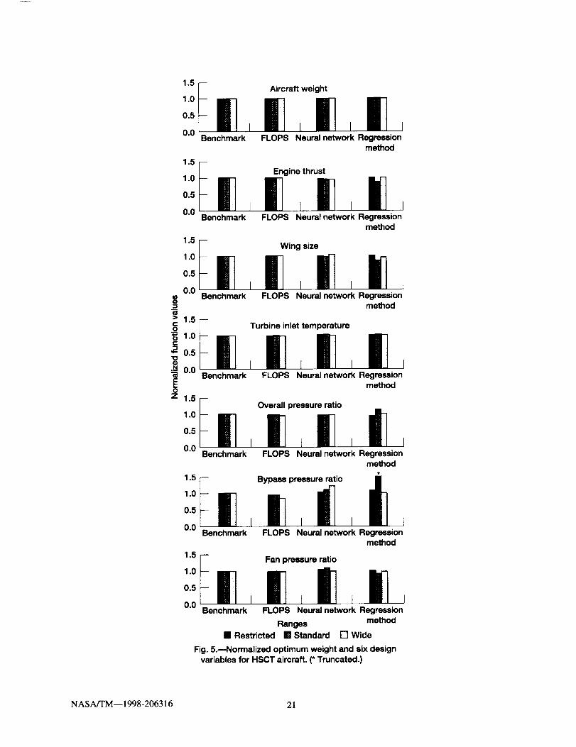
Closed-form gradients and finite difference gradients were used in the standard range to obtain the solutions shownin tables IX and X. The solutions in the wide range are presented in tables XI and XII. The solutions in all three

ranges (standard, wide, and restricted) are compared with the benchmark solution (see the barcharts in figs. 5 and 6).

The performance of the approximation methods in design optimization of the HSCT aircraft in the standard and

wide ranges is discussed separately with respect to the design variables, the merit function, the active constraints,

and the passive constraints.

Design Variables

The optimum results for the first four design variables (thrust, wing area, inlet temperature, and overall pressure

ratio), as determined with the neural network analyzer, differed from the benchmark solution by a maximum of

5 percent in the standard and wide ranges (see fig. 5). The maximum deviation obtained by this method for the other

two design variables (bypass and fan pressure ratios) was 10 percent in the standard range and 21 percent in the

wide range. Using the regression method in the standard range yielded a maximum deviation for the design variables

within 14 percent, except for the bypass pressure ratio, which was about 84 percent. The performance of the full

cubic polynomial regression method was unacceptable in the wide range. Thus, the regression approximator was

retrained with a quadratic polynomial in the design variables. The results are given in tables XI and XII. In the wide

range, the maximum deviation for the design variables was within 4 percent by this method.

Merit Function

The merit function was better behaved than the design variables in both ranges, except for an 11 percent devia-

tion obtained by the regression method in the standard range (see fig. 5).

Active Constraints

For the neural network method, the maximum deviation for the active constraints for both ranges was within

13 percent. With the regression method, the maximum deviation of 68 percent in the standard range was reducedto 4 percent when the regression approximator was retrained with quadratic basis functions in the wide range (see

fig. 6).

Passive Constraints

A large deviation was observed for the passive constraints in both the standard and wide ranges. For example,

the second-segment climb as determined by the neural network deviated by 1907 percent, and that determined by

the regression method deviated by 76 827 percent. Even though this constraint exhibited substantial deviation in the

restricted range, its performance in the standard and wide ranges can be considered unacceptable (see fig. 6).

Both regression and neural network methods gave similar optimization results, with some deviations, regardless

of whether closed-form or finite difference gradients were used.

NASA/TM--1998-206316 12

REFERENCES

1.Guptill,J.D.,Coroneos,R.M.,Patnaik,S.N.,Hopkins,D.A.,andBerke,L.,"CometBoardsUsersManual:Release1.0,"NASATM-4537,1996.

2. Patnalk,S.N.,Coroneos,R.M.,Guptill,J.D.,andHopkins,D.A.,"ComparativeEvaluationofDifferentOptimi-zationAlgorithmsforStructuralDesignApplications,"International Journal for Numerical Methods inEngineering, Vol. 39, 1996, pp. 1761-1774.

3. Patnaik, S.N., Guptill, J.D., and Berke, L., "Singularity in Structural Optimization," International Journal for

Numerical Methods in Engineering, Vol. 36, 1993, pp. 931-944.

4. Patnaik, S.N., Lavelle, T.M, Hopkins, D.A., and Coroneos, R.M., "Cascade Optimization Strategy for Aircraft

and Air-Breathing Propulsion System Concepts," Journal of Aircraft, Vol. 34, 1997, pp. 136-139.

5. McCullers, L.A., "Aircraft Configuration Optimization Including Optimized Flight Profiles," edited by

Sobieski, J., Symposium on Recent Experiences in Multidisciplinery Analysis and Optimization, part 1, NASACP-2327, 1984.

6. Patnalk, S.N., Guptill, J.D., and Berke, L., "Merits and Limitations of Optimality Criteria Method for Structural

optimization," International Journal for Numerical Methods in Engineering, Vol. 38, 1995, pp. 3087-3120.

7. "DOT User's Manual, Version 2.00," Engineering Design Optimization, Inc., Santa Barbara, CA, 1989.

8. Belegundu, A.D., Berke, L., and Patnaik, S.N., "An optimization Algorithm Based on the Method of Feasible

Directions," Structural Optimization, Vol. 9, 1995, pp. 83-88.9. Schittkowski, K., "User's Manual, FORTRAN Subroutines for Mathematical Applications, Version 2.0," IMSL,

Inc., Houston, TX, 1991.

10. Arora, J.S., "IDESIGN User's Manual Version 3.5.2," Optimal Design Laboratory, The University of Iowa,

Iowa City, IA, 1989.

11. "NAG FORTRAN Library Manual-MARK 15," NAG FORTRAN Library Routine Document, Downer'sGrove, IL, 1991.

12. Miura, H., and Schmit, L.A., Jr., "NEWSUMT--A FORTRAN Program for Inequality Constrained Function

Minimization, Users Guide," NASA CR-159070, 1979.

13. Gabriele, G.A., and Ragsdell, K.M., "OPT-A Nonlinear Programming Code in FORTRAN Implementing theGeneralized Reduced Gradient Method, User's Manual," University of Missouri-Columbia, 1984.

14. "RPK_NASTRAN," COSMIC, University of Georgia, Athens, GA, 1994.15. Nakazawa, S., "MHOST Version 4.2. Vol. 1: User's Manual," NASA CR-182235, 1989.

16. Venkayya, V.B., and Tischler, V.A., "ANALYZE: Analysis of Aerospace Structures With Membrane Ele-

ments," Report AFDL-TR-78-170, Air Force Flight Dynamics Laboratory, Wright-Patterson Air ForceBase, OH, 1978.

17. Patnaik, S.N., Hopkins, D.A., Aiello, R.A., Berke, L., "Improved Accuracy for Finite Element Structural Analy-

sis via a New Integrated Force Method," NASA TP-3204, 1992.

18. Plencner, R.M., and Snyder, C.A., "The Navy/NASA Engine Program (NNEP89)--A User's Manual," NASATM-105186, 1991.

19. Gendy, A.S., Patnaik, S.N., Hopkins, D.A., and Berke, L., "Parallel Computational Environment for Substruc-ture Optimization," NASA TM-4680, 1995.

20. Hafez, W.A., "Cometnet--User Manual," IntelliSys, Beachwood, OH, 1996.

21. Feagin, R.C., and Morrison, W.D., "Delta Method, An Empirical Drag Buildup Technique," NASACR-151971, 1978.

22. Sommer, S.C., and Short, B.J., "Free-Flight Measurements of Turbulent-Boundary-Layer Skin Friction in the

Presence of Severe Aerodynamic Heating at Math Numbers from 2.8 to 7.0," NACA TN-3391, 1955.

23. Geiselhart, K.A., "A Technique for Integrating Engine Cycle and Aircraft Configuration Optimization," NASACR-191602, 1994.

24. Geiselhart, K.A., Caddy, M.J., and Morris, S.J., Jr., "Computer Program for Estimating Performance of Air-

Breathing Aircraft Engines," NASA TM--4254, 1991.

25. Caddy, M.J., and Shapiro, S.R., "NEPCOMP--The Navy Engine Performance Computer Program, Version I,"NADC-74045-30, 1975.

NASA/TM-- 1998-206316 13

26. Clark, B.J., "Computer Program To Predict Aircraft Noise Levels," NASA TP-1913, 1981.

27. Johnson, V.S., "Life Cycle Cost in the Conceptual Design of Subsonic Commercial Aircraft," Ph.D. Thesis,

Univ. of Kansas, Lawrence, KS, 1989.

28. Eide, D.G., "Cost Estimating Relationships for Airframes in the Development and Production Phases," NASA

TM-80229, 1980.

29. Beltramo, M.N., Trapp, D.L., Kimoto, B.W., and Marsh, D.P., "Parametric Study of Transport Aircraft Systems

Cost and Weight," NASA CR-151970, 1977.

30. Nelson, J.R., and Timson F.S., "Relating Technology to Acquisition Costs: Aircraft Turbine Engines,"

R-1288-R, Rand Corp., Santa Monica, CA, 1974.

31. "A New Method for Estimating Current and Future Transport Aircraft Operating Economics," American Air-

lines, NASA CR-145190(rev.), 1978.

32. Stoessel, R.F., "A Proposed Standard Method for Estimating Airline Indirect Operating Expenses," CN-150,

Logistic Distro-Data, Inc., 1970.

33. Anderson, E., et al., "LAPACK User's Guide," Society for Industrial and Applied Mathematics, Philadelphia,

PA, 1992.

34. Press, W., Teukolsky, S., Vetterling, W., and Flannery, B, "Numerical Recipes Example Book (C)," Cambridge

University Press, NY, 1987.

35. Rissanen, J., "Stochastic Complexity," Journal of the Royal Statistical Society, Series B--Methodological,

Vol. 49, 1987, pp. 223-239.

Related sets

1

2

3

4

TABLE I.--DESIGN VARIABLE SELECTION STRATEGY

Active design variables Influence re_ion Variables in desi[_n zonesNumber Variables Number Sets Number Variables

2 4,7 1 2 3 2,4,7

1 2 3 1,3,4 6 1,2,3,4,5,7

2 3,5 2 2,4 5 1,2,3,5,7

3 1,2,7 2 2,3 5 1,2,3,5,7

Number

TABLE II--DESIGN VARIABLES AND THEIR RANGES FOR THE

HSCT AIRCRAFT

De_fiption Status Lower

I Ramp wei[,ht, lb

2 Win_ aspect ratio

3 Engine thrust, lb

4 Taper ratio of wing5 Wing area, ft 2

Passive

Passive

Active

Passive

Active

6 Sweep an[le, de[ Passive

7 Win[ thickness-chord ratio Passive8 Cruise Mach number Passive

9 Maximum cruise altitude, ft Passive

10 Turbine entry temperature, °R Active

11 Overall pressure ratio Active

12 Bypass ratio Active

13 IFan pressure ratio Active

14 Engine throttle ratio Passive

_Range outside training range.

bTraining range of approximating analyzers.

CRestricted range inside training range.

Initial Upper bound

bound design

.... 2.363 ....

a30 000 "50000 170 000

b36 000 M1 000 b45 000

c40 500 ¢41 000 c41 500

0.057

a7 0(!O 18000 _12 000

b7 100 b8 100 b9 100

¢8000 c8 100 c9000

62.224 ....

.... 0.03 ....

.... 2.4 ....

.... 70 000 ....

_2 300 a3 000 R3 560

b2 300 b2 900 b3 500

¢2 850 c2 900 _3 000

"15 *24 * 30

b18 b21 b25

_20 ¢21 c22

• 0.10 " 0.25 a 0.8

b0.25 b0.40 b0.8

_0.39 _0.40 ¢0_5

"1.2 *3.6 _4.8

b2.6 b3.6 b4.6

¢3.5 ¢3.6 ¢3.8

1.126

NASA/TM--1998-206316 14

TABLE I]].--OPTIMUM WEIGHT FOR HSCT FOR THE FIVE TEST CASES

Test cases NASA CometBoards solution Industr_ solution

Weight, lb Deviation, percent

678 450.1

5 (benchmark)

Weight, Ib Deviation,

percent666 529.0 0.00

666 578.4 0.00

677 264.1 1.60

666 526.5 0.00

666 530.9 0.00

1

2 666 730.0

3 667 064.0

4 666 658.0

666 665.0

1.79

0.02

0.08

0.02

0.02

TABLE IV.--BENCHMARK SOLUTION FOR THE HSCT AIRCRAFT

Parameters

Aircraft weight, lb

Initial CometBoards Industry

desil_n solution solution753 395.2 666 530.9 666 665.0

Active desi :n variables

(1) Engine thrust, Ib

(2) Wing size, ft 2

(3) Turbine inlet temperature, °R

(4) Overall pressure ratio

(5) Bypass pressure ratio

(6) Fan pressure ratio

50 000.0

7 000.0

3 200.0

18.0

0.7

2.5

41 417.730 41 494.690

8 169.750 8 161.780

2 957.810 2 957.790

21.618 21.627

0.434 0.437

3.619 3.593

Behavior constraints

(1) Missed approach thrust, lb

(2) Second-segment climb thrust, lb

(3) Landing approach velocity, kn

(4) Take off field length, tt

(5) Jet velocity, kn

(6) Compressor discharl_e temperature, °R

Number of reanalyses to solution

87 718.0

12 968.0

169.0

13 742.0

2 107.7

1 586.8

71 028.760

24.502

147.150

11 000.200

2 300.000

1 709.990

134

71 174.0

279.0

147.2

11 000.0

2 287.9

1 709.5

1240

TABLE V.--PERCENT MEAN ERROR IN THE THREE RANGES

Response quantities

Weight

Missed approach

Second-segmentclimb

Approach velocit]¢

Takeoff field len_th

Jet velocit),

Compressor

temperature

Mean error, percent

Restricted range Standard range

Regression Neural Regression Neuralmethod network method network

0.439 0.928 2.224 2.560

0.021 0.069 0.253 0.311

3.441 2.413

0.194 0.523

1.755 5.1 95

0.203 0.675

0.264 0.553

Wide range

Regression method

Cubic Quadraticfunction function

1 375 7.123

128 0.534

17.20 3 10.215 9 720 110

1.082 1.499 753 0.422

13.509 13.623 8 180 109

0.534 3.016 157 0.949

1.938 1.753 53 2.427

Neural

network

6.743

3.367

110

6.967

65.794

9.762

7.326

NASA/TM-- 1998-206316 15

TABLEVI.--HSCTAIRCRAFTDESIGNUSINGAPPROXIMATIONS IN RESTRICTED RANGE WITH

CLOSED-FORM GRADIENTS

Design parameters Benchmark

Aircraft weight, lb

solution

FLOPS

analyzer666530.9 0.11

Active desi[n variables

En[_ine thrust, lb

Win[ size, ft 2

Turbine inlet temperature, °R

Overall pressure ratio

Bypass pressure ratio

Fan pressure ratio

41 417.730 I 0.03

8 169.750 0.14

2 957.810 -0.66

21.618 -2.07

0.434 -6.24

3.619 -1.74

Behavior constraints

Missed approach thrust, lb 71 028.760

Second-se[ment climb thrust, lb 24.502

Landin_ approach velocit?, kn 147.150

Takeoff field length, fi 11 000.200

Jet velocity, kn 2 300.000

Compressor discharge

temperature, °R 1 709.990

"Values were generated by FLOPS analyzer for the o

and regression methods.

-0.08

-100.00

-0.01

0.11

-0.53

Percent deviation in optimum solution

Neural network Regression

0.81 I '0.17 0.98 I "0.65

-2.22 -2.22 0.20 0.20

0.32 0.32 1.29 1.29

1.77 1.77 1.77 1.77

-3.47 -3.47 -5.36 -5.36

3.27 3.27 7.60 7.60

5.00 5.00 1.20 1.20

-3.74 "-3.77 -0.13 a0.08

1 706.05 "-99.90 760.78 _-99.94

-0.12 "-0.07 -0.15 "-0.31

0.00 "4.70 0.130 "0.04

0.00 "0.93 0.00 '0.36

0.00 0.00 "-0.99 - 1.85 a_2.18

_timum designs that were obtained by neural network

TABLE VII.--HSCT AIRCRAFT-DESIGN USING APPROXIMATIONS IN RESTRICTED RANGE

WITH FINITE DIFFERENCE GRADIENTS

Design parameters

Aircraft wei[ht, lb

En[ine thrust, lb

Win[ size, ft 2

Turbine inlet temperature, °R

Overall pressure ratio

B_lpass pressure ratio

Fan pressureratio

Missed approach thrust, lb

Second-se[gment climb thrust, lb

Landin[ approach velocit_¢, kn

Takeoff field len[th, ft

Jet velocit),, kn

Compressor discharge

Benchmark Percent deviation in optimum solutionsolution

FLOPS Neural network

analyzer

666 530.9 0.11 0.84 I "0.45

Active design variables41 417.73 0 0.03 -2.22 -2.22

8 169.750 0.14 2.06 2.06

2 957.81 0 -0.66 1.77 1.77

21.618 -2.07 -3.38 -3.38

0.434 -6.24 2.44 2.44

3.619 -1.74 5.00 5.00

Behavior constraints

71 028.760 -0.08 -3.28 a-3.78

24.502 -100.00 1 290.96 "- 100.00

147.150 -0.01 -0.99 *0.79

11 000.200 0.11 -3.34 "3.79

2 300.00 0 -0.53 0.00 "1.07

1 709.990 0.00 0.00 a-l.00

Regression

0.98 I "0.66

0.20 0.20

1.27 1.27

1.77 1.77

-5.46 -5.46

7.58 7.58

1.07 1.07

-0.11 _0.08

751.39 "-99.94

•0.14 "-0.30

0.00 "0.07

0.00 "0.37

-I.88 "-2.25

temperature, °R

"Values were generated by FLOPS analyzer for the optimum designs that were obtained by neural

network and regression methods.

TABLE VIlI._PU TIME FOR DESIGN OPTIMIZATION ON A SILICON GRAPHICS PS 480-VGX

[ALL TIMES ARE GIVEN IN SECONDS .

Activity FLOPS Neural network

Closed-form Closed-form

_radients _radients

User S?stem User S?stem

Generation of io-pairs -- 63 207 827

Traininl_ -- 2 407 16.8

Optimization 8 897 96 24.1 40.3

Finite difference

sradients i

User S_'stem

(a) (b)

(c) (d)

124.4 263.5

Re_ression anal?sisClosed-form Finite difference

_adients" _radients"

User S_,stem User S?stem(a) (b) (a) (b)

2.2 0.2 (e) (f)

0.4 0.1 1.9 0.2

aNote: (a) and (b) generation of io pairs was carried out only once; (c) to (f) neural network and regression methods weregained once.

NASA/TM-- 1998-206316 16

TABLE IX. --HSCT AIRCRAFT DESIGN USING APPROXIMATIONS IN STANDARD RANGEWITH CLOSED-FORM GRADIENTS

Design parameters Benchmark Percent deviation in optimum solutionsolution

FLOPS Neural network

Aircraft wei[ht, lb

Engine thrust, lb

Win_ size, ft 2

Turbine inlet temperature, °R

Overall pressure ratio

B_ass pressure ratio

i Fan pressure ratio

Missed approach thrust, lb

Second-segment climb thrust, lb

Landin_ approach velocit]t, kn

Takeoff field ien[th, ft

IJet velocity,, kn

Compressor discharge

temperature, °R

Regression

anal_,zer

666530.9 0.03 -1.17 I "-0.088 -10.75 I "1.61

Active design variables41 417.730 -0.06 -4.52 -4.52 -13.08 -13.08

8 169.750 0.12 -2.65 -2.65 -13.09 -13.09

2 957.81 0 -0.24 2.81 2.81 3.2.6 3.26

21.618 -1.20 -3.87 -3.87 13.69 13.69

0.434 -6.41 10.02 10.02 84.33 84.33

3.619 -0.60 10.21 10.21 -7.88 -7.88

Behavior constraints

71 028.760 -0.10 -6.66 ' -7.93 -11.60 '-26.58

24.502 20.81 1907.67 "-99.94 76 827.00 "-99.97

147.150 -0.04 0.49 " 1.31 2.21 "8.13

11 000.200 0.00 0.00 "12.66 -3.82 '67.81

2 300.000 0.01 0.00 "0.88 -12.88 "-9.79

1 709.990 0.02 0.00 "-0.95 0.00 "1.56

aValues were generated by FLOPS analyzer for the optimum designs that were obtained by neural

network and regression methods.

TABLE X.--HSCT AIRCRAFT DESIGN USING APPROXIMATIONS IN STANDARD RANGE WITHFINITE DIFFERENCE GRADIENTS

Design parameters

Aircraft wei[;ht, lb

En[ine thrust, lb

Win[ size, ft 2

Turbine inlet temperature, °R

Overall pressure ratio

B]cpass pressure ratio

Fan pressure ratio

Missed approach thrust, lb

Second-seE;ment climb thrust, Ib

Landin[ approach velocity, kn

Takeoff field lenbnh, ft

Jet velocity,, kn

Compressor discharge

temperature, *R

Benchmark

solution

FLOPS Neural network

anal),zer

666530.9 0.03 -1.16 [ =-0.11

Active desi[n variables41 417.730 -0.06 -4.60 -4.60

8 169.750 0.12 -2.56 -2.56

2 957.81 0 -0.24 2.67 2.67

21.618 -1.20 -4.11 -4.11

0.434 -6.41 9.06 9.06

3.619 -0.60 9.87 9.87

Behavior constraints

71 028.760 -0.10 -6.71 "-8.03

24.502 20.81 1 868.90 "-99.90

147.150 -0.04 0.40 =1.25

11 000.200 0.00 0.00 =12.63

2 300.000 0.01 0.(30 '0.90

Percent deviation in optimum solution

Regression

-14.92 I "-0.71

-13.08 -13.08

-13.09 -13.09

4.99 4.99

15.64 15.64

11.45 11.45

9.10 9.10

1 709.990 0.02 0.00 "-0.%

that were"Values were generated by FLOPS analyzer for the optimum designs

network and regression methods.

-9.32 "-23.02

64 369.61 "- 100.00

0.09 '6.89

-4.19 "50.34

0.00 "2.75

0.00 "1.12

obtained by neural

NASA/TM-- 1998-206316 17

TABLEXI.--HSCTAIRCRAFTDESIGNUSINGAPPROXIMATIONS IN WIDE RANGE WITH

CLOSED-FORM GRADIENTS

Design parameters

Aircraft weight, lb

Ent:ine thrust, lb

Win[g size, ft 2

Turbine inlet temperature, °R

Overall pressure ratio

Bypass pressure ratio

Fan pressure ratio

Benchmark

solutionPercent deviation in optimum

FLOPS Neural network

I b0"77

solution

Regression "

anal),zer

666 530.9 0.50 -0.24 0.25 I b0"21

Active desiE:n variables41 417.730 0.40 -4.82 -4.82 0.65 0.65

8 169.750 0.47 430 4.30 -3.87 -3.87

2 957.810 -1.74 0.53 0.53 1.68 1.68

21.618 -5.15 -2.51 -2.51 0.98 0.98

0.434 -15.76 21.61 21.61 0.85 0.85

3.619 -1.92 -0.59 -0.59 -1.41 -1.41

Behavior constraints

71 028.760 -0.75 b0.69

24.502 4 797.35 b6 244.23

147.150 2.22 b2.10

11 000.200 0.00 b4.24

2 300.000 0.00 b0.45

Missed approach thrust, lb 0.41 -8.66 b-9.03

Second-se[ment climb thrust, ft -100.00 534.26 b-100.00

Landin[_ approach velocit_¢, kn 0.02 -2.70 b-l.70

Takeoff field length, ft 0.02 0.(30 b9.59

Jet velocity, kn -0.12 -4.55 b-3.63

Compressor discharge

temperature, °R 1 709.990 0.00 0.00 b0.00 0.00 b-0.37

aRegression analysis in the wide range was found to be satisfactory only for quadratic approximations

in design variables.bValues were generated by FLOPS analyzer for the optimum designs that were obtained by neural

network and regression methods.

TABLE XII.--H SCT AIRCRAFT DESIGN USING APPROXIMATIONS IN WIDE RANGE WITH FINITE

DIFFERENCE GRADIENTS

Design parameters

Aircraft weight, Ib

En[ine thrust, lb

Win[ size, ft 2

Turbine inlet temperature, °R

Overall pressure ratio

Bypass pressure ratio

Fan pressureratio

Benchmark

solutionPercent deviation in optimum solution

FLOPS Neural network Regression i

anal),zer

666 530.9 0.50 -2.07 I 0.07 0.25 I b0"24

Active desii:n variables41 417.730 0.40 -1.65 -1.65 0.54 0.54

8 169.750 0.47 -8.32 -8.32 -3.68 -3.68

2 957.810 -1.74 2.04 2.04 1.58 1.58

21.618 -5.15 -9.85 -9.85 0.79 0.79

0.434 -15.76 29.98 29.98 0.09 0.09

3.619 -1.92 -7.12 -7.12 -1.61 -1.61

Behavior constraints

71 028.760 b0.50

24.502 b5 433.24

147.150 b2.02

11 000.200 b4.20

2 300.000 b0.43

Missed approach thrust, lb 0.41 -1.69 b-4.18 0.59

Second-se[ment climb thrust, lb -100.00 4 671.64 b-99.90 4 596.95

l_,andin_ approach velocit)', kn 0.02 3.29 b4.48 2.12

Takeoff field length, fi 0.02 0.00 b13.71 0.00

Jet velocit_¢, kn -0.12 -4.36 b-3.40 0.00

Compressor discharge

temperature, °R 1 709.990 0.00 -5.28 b-3.65 0.00 b-0.34

"Regression analysis in the wide range was found to be satisfactory only for quadratic approximations in

design variables.

bVaiues were generated by FLOPS analyzer for the optimum designs that were obtained by neural network

and regression methods.

NASA/TM-- 1998-206316 18

Fig. 1 .--Organization of CometBoards test bed.

{2}

_._ {3,5}

Fig. 2._Dseign vadable sets with influence regions.

Circled numbers represent sets; braced numbers are

active design variables, Adjacent regions are

coupling regions.

NASA/TM-- 1998-206316 19

10.0

9.0

ii• •

_ 6.0

> 5.0

g•_ 4.0 •

L" ".'_ . "a 3o_ .,. . = .

zo_ .,-. : t. .. . .

1.0_ " °I I 1 "I" I0.0 I T i I0.0 1.0 2.0 3.0 4.0 5.0 6.0 7.0 8.0 9.0 10.0

Design variable 1

Fig. 3.mlnput portion of io-palrs for two design variables

(Id = initial design).

"O

m

O

z0.9

0.8 a)33

I36

Analyzer

FLOPS

.... Neural network

....... Regression method

I I I I39 42 45 48x103

Engine thrust, Ib

1,2 m

1.1

._m

1.0

0

z0.9

• //, /

.'//

_f

Analyzer

- FLOPS

.... Neural network

....... Regression method

0.8 (b) l I I I I ] L I I70 73 76 79 82 85 88 91 94 97x102

Wing area, ft2

Fig. 4.--Aircraft weights obtained by using approxima-

tions and FLOPS analyzer (a) as a function of engine

thrust and (b) as a function of wing area.

NASA/TM-- 1998-206316 20

1.5 ._

1.0

0.5

o.o __1Benchmark FLOPS Neural network Regression

method

1 B5 F| Engine thrust

0.5

0.o I | I |Benchmark FLOPS Neural network Regression

method

0,51"5f_1"0 Wingsize _r_

o.0 I I I I= Benchmark FLOPS Neural network Regression

method

1.5 Turbine inlet temperature1,0

0.5

0.0 I I I |Benchmark FLOPS Neural network Regression

o_ method

z 1.5

1.00.5

0.0Benchmark FLOPS Neural network Regression

method

1.0

0.5

0.0Benchmark FLOPS Neural network Regression

method

1.01"5f _ Fan pressure rati__J]0.5

0.0 I 1 | |Benchmark FLOPS Neural network Regression

Ranges method

• Restricted [] Standard [] Wide

Fig. 5.--Normalized optimum weight and six designvariables for HSCT aircraft. (* Truncated.)

NASA/TM--1998-206316 21

1.0

0.5

0.0Benchmark FLOPS Neural network Regression

_thod

okfOSc°is mentcm}I ** I * I I

0.0 Benchmark FLOPS Neural network Regressionmethod

1.5 Landing approach velocity

0.5

•_ 0.0 Benchmark FLOPS Neural network Regressionmethod

_ 0.5

0.0Benchmark FLOPS Neural network Regression

method

11.0 _ __0.5"5f Jet velocity

0.0_ I I I IBenchmark FLOPS Neural network Regression

method

1.0

0.5

0.0Benchmark FLOPS Neural network Regression

method

Ranges

• Restricted IB Standard I-I Wide

Fig. 6.--Normalized constraint values at the optimumfor HSCT aircraft. (*Padded or truncated.)

NASA[I'M-- 1998-206316 22

REPORT DOCUMENTATION PAGE FormApprovedOMB No. 0704-0188

Public reporting burden for this collection of information is estimated to average 1 hour per response, including the time for revrewing instructions, seamhing existing data sources,gathering and maintaining the date needed, and completing and reviewing the collection of information. Send comments regarding this burden estimate or any other aspect of thisco,action of information, including suggestions for reducing this burden, to Washington Headquarters Services, Directorate for Information Operations and Reports, 1215 JeffersonDavis Highway, Suite 1204, Arlington, VA 22202-4302, and to the Office of Management and Budget, Paperwork Reduction Project (0704-0188), Washington, DC 20503.

1. AGENCY USE ONLY (Leave blank) 2. REPORT DATE 3. REPORT TYPE AND DATES COVERED

April 1998 Technical Memorandum4. TITLE AND SUBTITLE 5. FUNDING NUMBERS

Neural Network and Regression Approximations in High Speed Civil Transport

Aircraft Design Optimization

6. AUTHOR(S)

Surya N. Patniak, James D. Guptill, Dale A. Hopkins, and Thomas M. Lavelle

7. PERFORMING ORGANIZATION NAME(S) AND ADDRESS(ES)

National Aeronautics and Space Administration

Lewis Research Center

Cleveland, Ohio 44135-3191

9. SPONSORING/MONITORING AGENCY NAME(S) AND ADDRESS(ES)

National Aeronautics and Space Administration

Washington, DC 20546-0001

WU-523-22-13-00

8. PERFORMING ORGANIZATION

REPORT NUMBER

E-10872

10. SPONSORING/MONITORING

AGENCY REPORT NUMBER

NASA TM--1998-206316

11. SUPPLEMENTARY NOTES

Surya N. Patnaik, Ohio Aerospace Institute, 22800 Cedar Point Road, Cleveland, Ohio 44142; James D. Guptill, Dale A.

Hopkins, and Thomas M. Lavelle, NASA Lewis Research Center. Responsible person, Surya N. Patnaik, organization code

5910, (216) 433-5213.

1211. DISTRIBUTION/AVAILABILITY STATEMENT

Unclassified - Unlimited

Subject Category: 64 Distribution: Nonstandard

This publication is available from the NASA Center for AeroSpace Information, (301) 621--0390

12b. DISTRIBUTION CODE

13. ABSTRACT (Meximum 2OO words)

Nonlinear mathematical-programming-based design optimization can be an elegant method. However, the calculations required to

generate the merit function, consa'aints, and their gradients, which are frequently required, can make the process computationally

intensive. The computational burden can be greatly reduced by using approximating analyzers derived from an original analyzer

utilizing neural networks and linear regression methods. The experience gained from using both of these approximation methods in the

design optimization of a high speed civil transport aircraft is the subject of this paper. The Langley Research Center's Flight Optimiza-

tion System was selected for the aircraft analysis. This software was exercised to generate a set of training data with which a neural

network and a regression method were trained, thereby producing the two approximating analyzers. The derived analyzers were

coupled to the Lewis Research Center's CometBoards test bed to provide the optimization capability. With the combined software, both

approximation methods were examined for use in aircraft design optimization, and both performed satisfactorily. The CPU time for

solution of the problem, which had been measured in hours, was reduced to minutes with the neural network approximation and to

seconds with the regression method. Instability encountered in the aircraft analysis software at certain design points was also elimi-

nated. On the other hand, there were costs and difficulties associated with training the approximating analyzers. The CPU time required

to generate the input-output pairs and to train the approximating analyzers was seven times that required for solution of the problem.

14. SUBJECT TERMS

Supersonic aircraft; Neural network; Design; Optimization; Regression; Analysis

17. SECURITY CLASSIFICATION

OF REPORT

Unclassified

NSN 7540-01-280-5500

18. SECURITY CLASSIFICATION

OF THIS PAGE

Unclassified

15. NUMBER OF PAGES

2816. PRICE CODE

A0319. SECURITY CLASSIFICATION 20. LIMITATION OF ABSTRACT

OF ABSTRACT

Unclassified

Standard Form 298 (Rev. 2-89)

Prescribed by ANSI Std. Z39-18298-102