70
Neural Network – Back-propagation HYUNG IL KOO
Neural Network –
Back-propagationHYUNG IL KOO
Hidden Layer Representations
• Backpropagation has an ability to discover useful intermediate
representations at the hidden unit layers inside the networks which
capture properties of the input spaces that are most relevant to
learning the target function.
• When more layers of units are used in the network, more complex
features can be invented.
• But the representations of the hidden layers are very hard to
understand for humans.

Basic Math
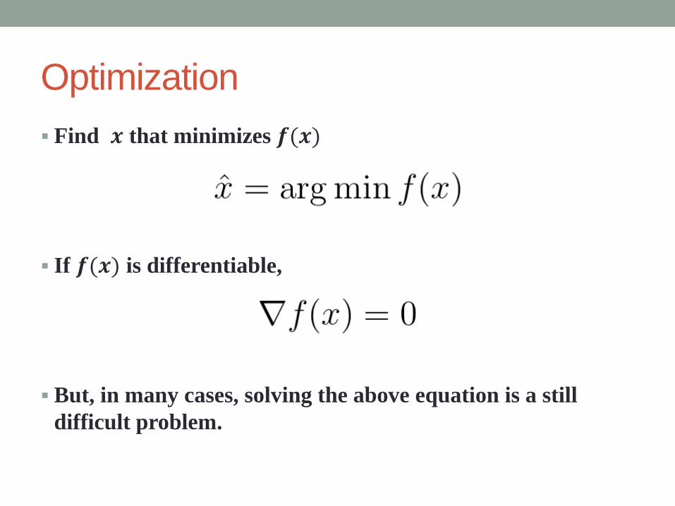
Optimization
Find 𝒙 that minimizes 𝒇(𝒙)
If 𝒇(𝒙) is differentiable,
But, in many cases, solving the above equation is a still
difficult problem.
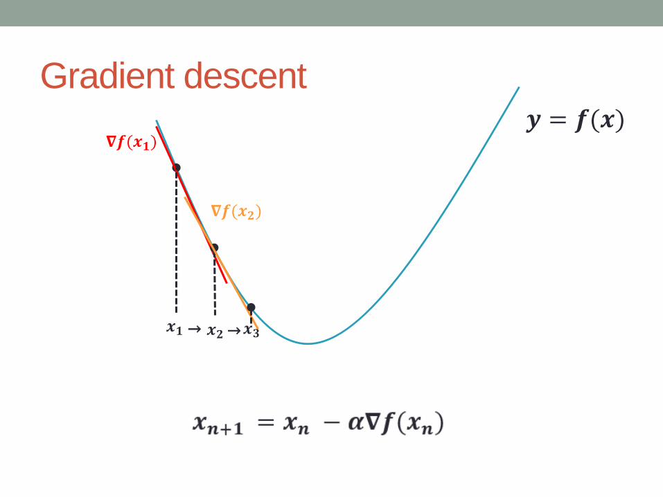
Gradient descent
𝛁𝒇(𝒙𝟏)
𝒙𝟏 𝒙𝟐
𝒚 = 𝒇(𝒙)
→
𝛁𝒇(𝒙𝟐)
𝒙𝟑→
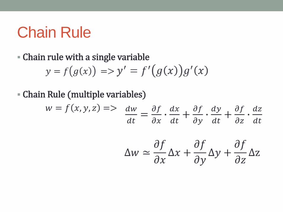
Chain rule with a single variable
Chain Rule (multiple variables)
𝑤 = 𝑓 𝑥, 𝑦, 𝑧 =>
Chain Rule
𝑑𝑤
𝑑𝑡=
𝜕𝑓
𝜕𝑥∙𝑑𝑥
𝑑𝑡+
𝜕𝑓
𝜕𝑦∙𝑑𝑦
𝑑𝑡+
𝜕𝑓
𝜕𝑧∙𝑑𝑧
𝑑𝑡
Δ𝑤 ≃𝜕𝑓
𝜕𝑥Δ𝑥 +
𝜕𝑓
𝜕𝑦Δ𝑦 +
𝜕𝑓
𝜕𝑧Δz
Feed-forward neural network
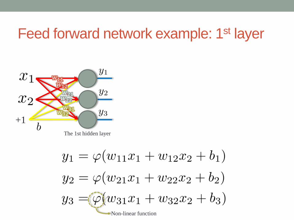
Feed forward network example: 1st layer
The 1st hidden layer
+1
Non-linear function
𝑤11𝑤12𝑤21𝑤22
𝑤31𝑤32
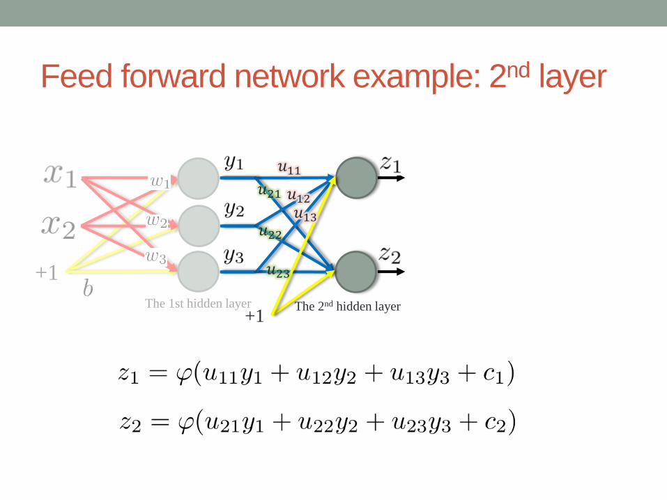
Feed forward network example: 2nd layer
The 2nd hidden layer+1
𝑢11
𝑢12𝑢13
𝑢23
𝑢22
𝑢21
The 1st hidden layer
+1
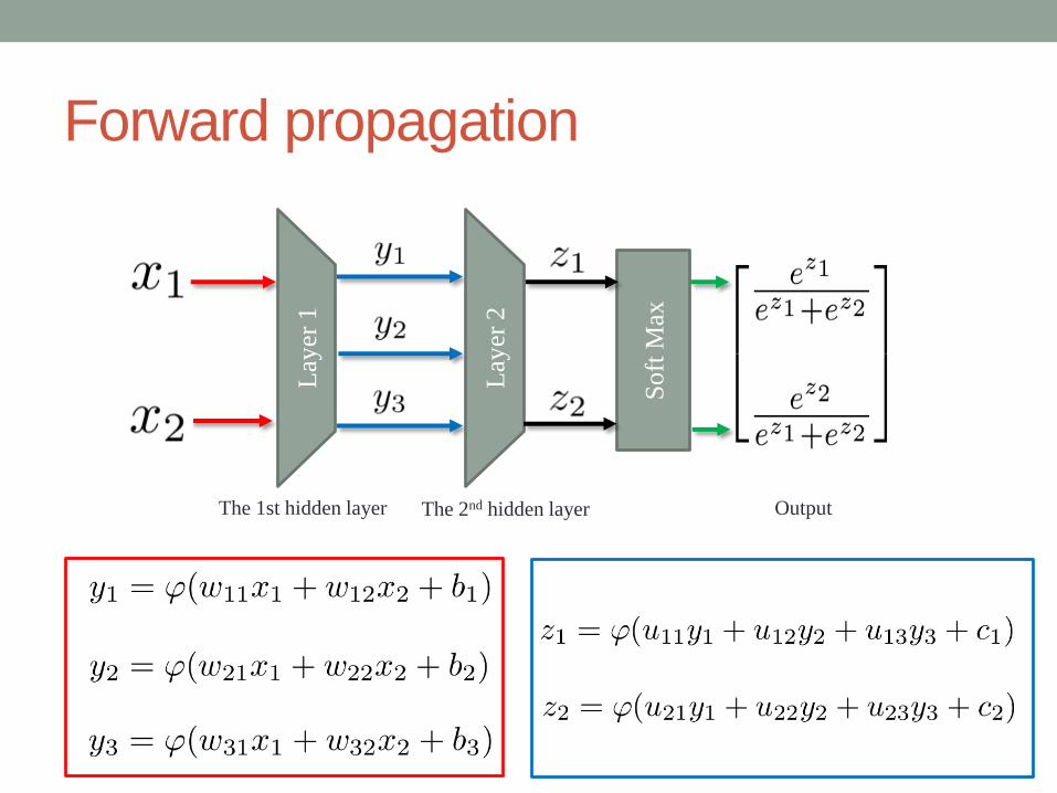
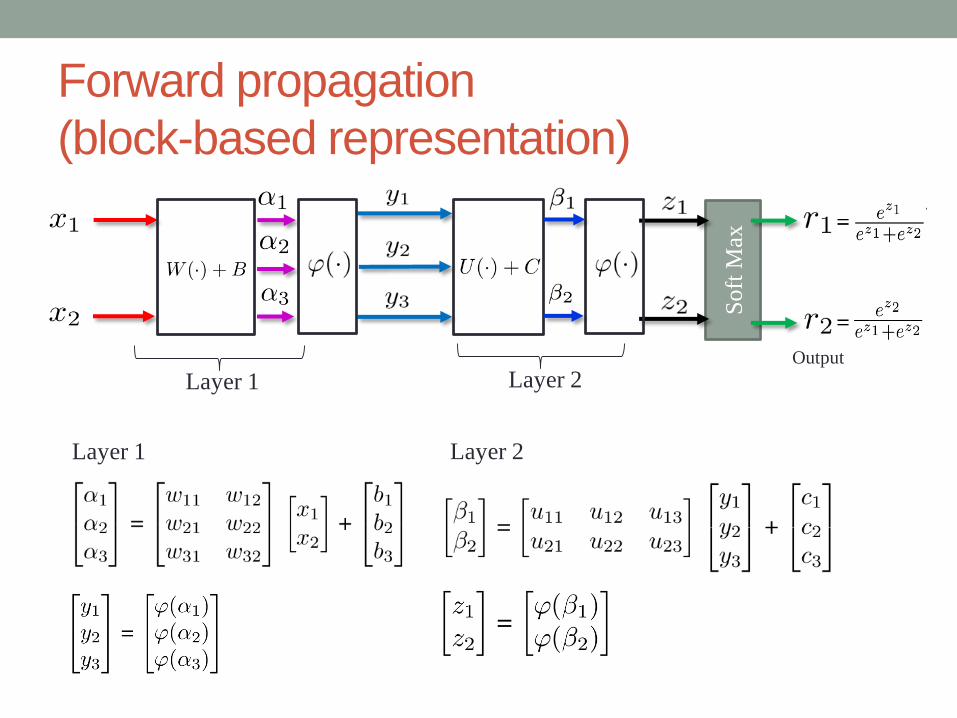
Forward propagation
The 1st hidden layer The 2nd hidden layer
Soft
Max
Lay
er 1
Lay
er 2
Output
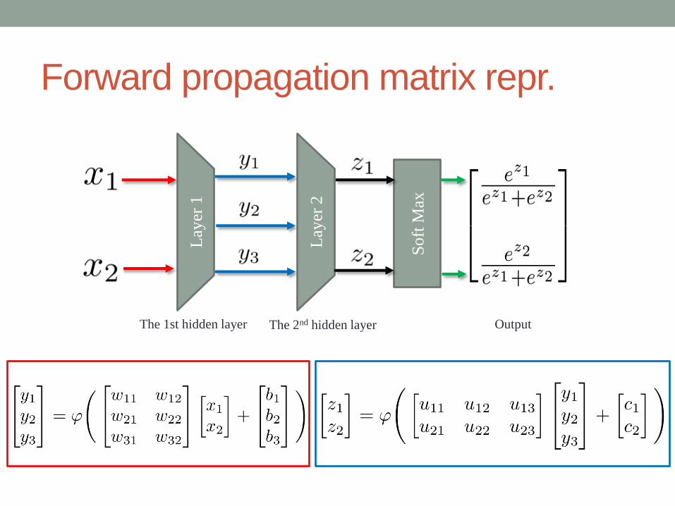
Forward propagation matrix repr.
The 1st hidden layer The 2nd hidden layer
Soft
Max
Lay
er 1
Lay
er 2
Output
Back-propagation algorithm
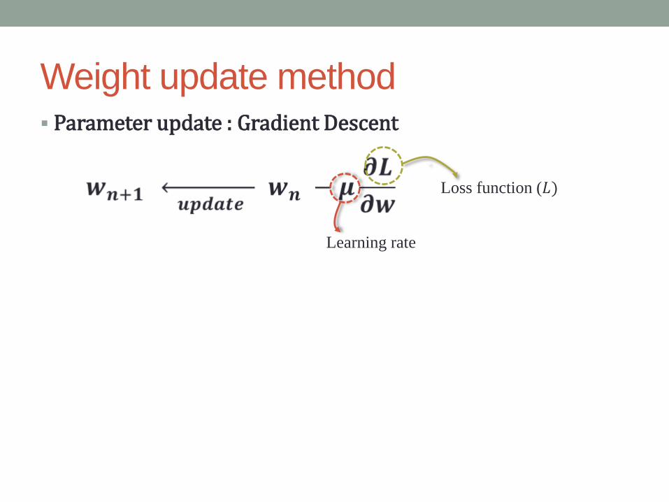
Parameter update : Gradient Descent
Weight update method
Learning rate
Loss function (𝐿)`
Ground Truth
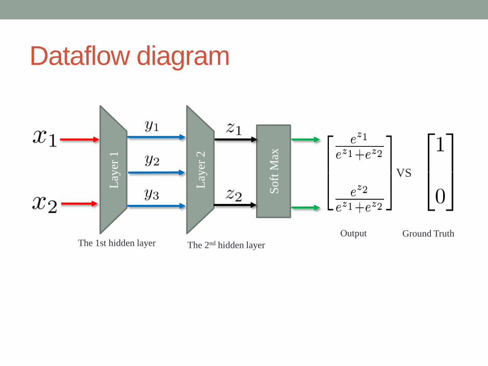
Dataflow diagram
The 1st hidden layer The 2nd hidden layer
Soft
Max
Output
Lay
er 1
Lay
er 2
VS
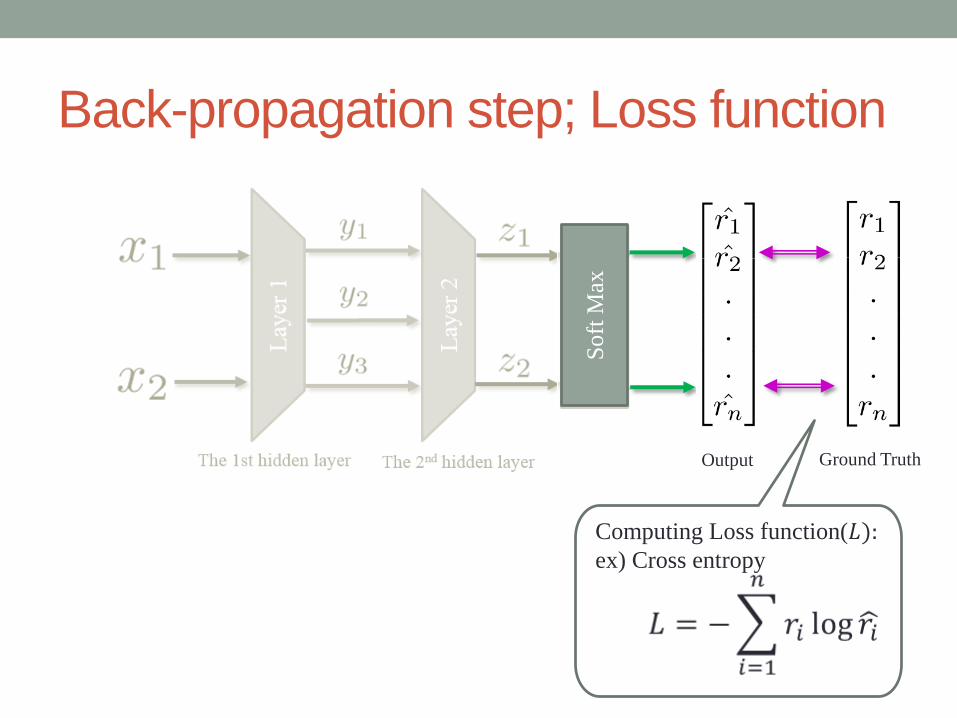
Back-propagation step; Loss function
Computing Loss function(𝐿):ex) Cross entropy
Soft
Max
Output Ground Truth
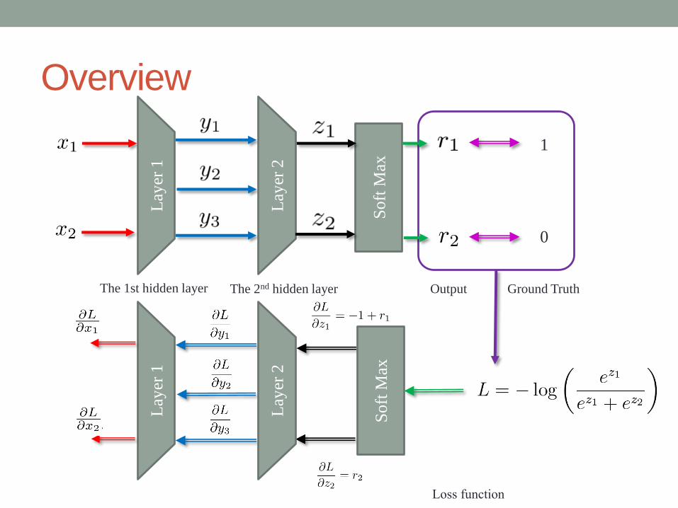
Overview
Lay
er 1
Lay
er 2
The 1st hidden layer The 2nd hidden layer
Soft
Max
Lay
er 1
Lay
er 2
Output Ground Truth
Loss function
1
0
Soft
Max
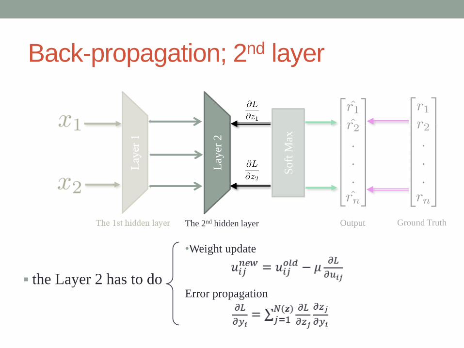
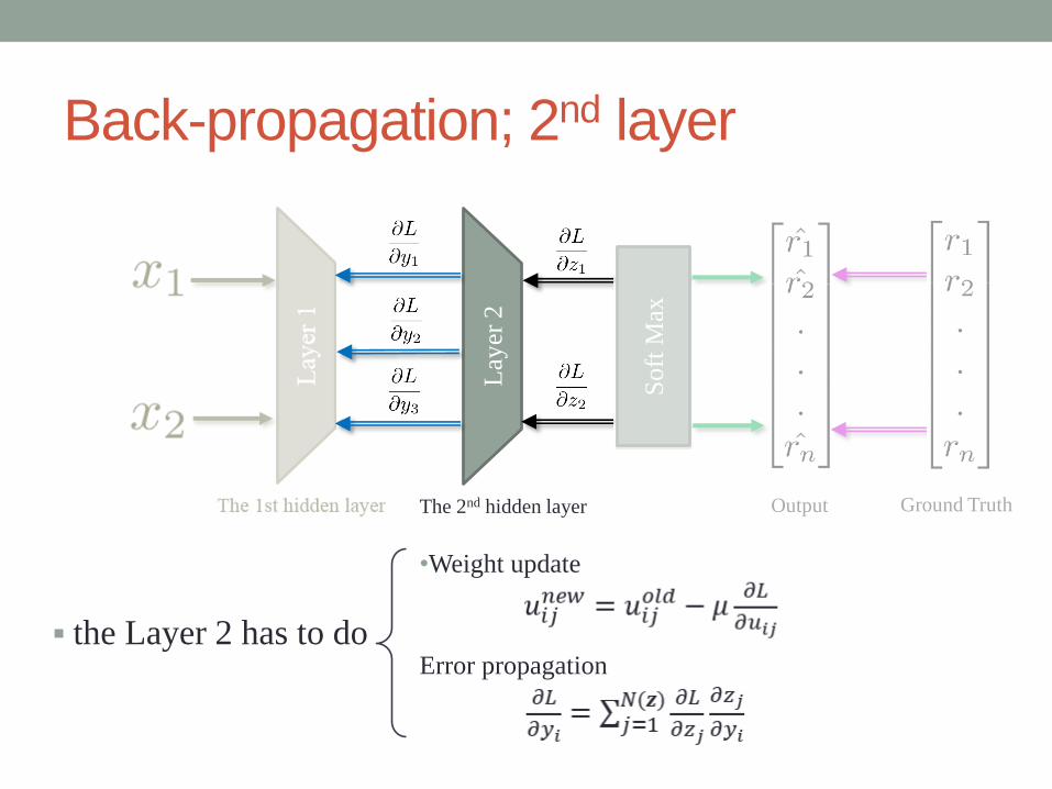
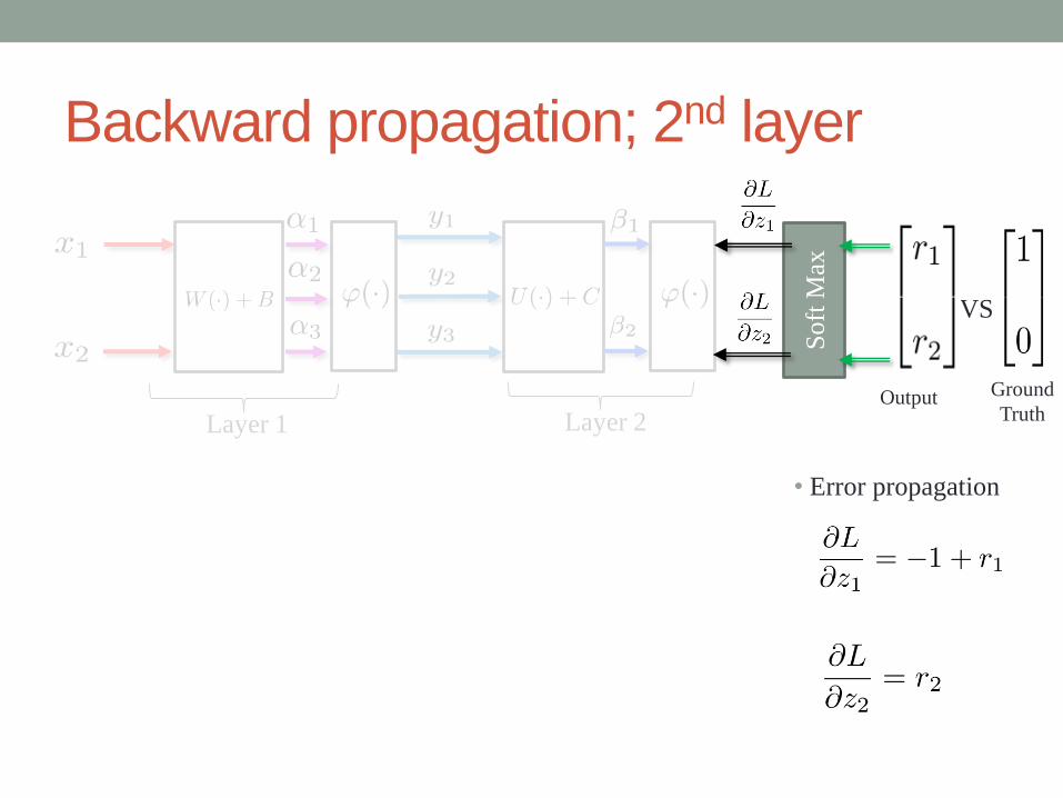
Back-propagation; 2nd layer
the Layer 2 has to do
Lay
er 2
The 1st hidden layer The 2nd hidden layer
Soft
Max
Output Ground Truth
•Weight update
Error propagation
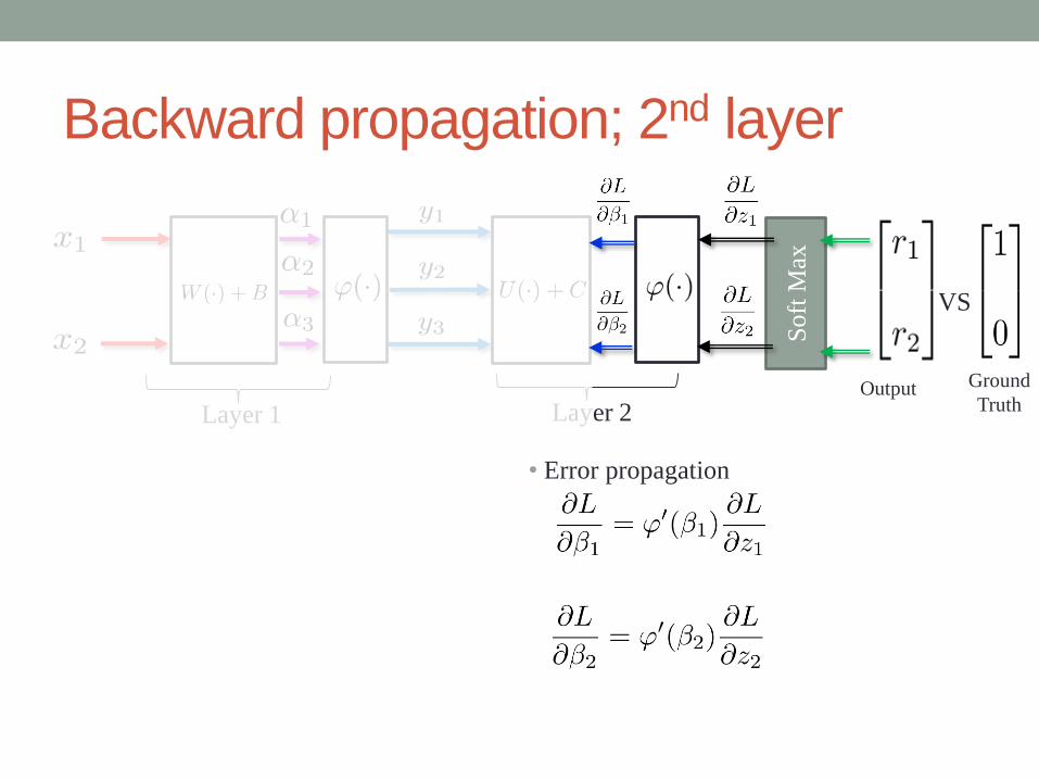
Back-propagation; 2nd layer
the Layer 2 has to do
Lay
er 2
The 1st hidden layer The 2nd hidden layer
Soft
Max
Output Ground Truth
•Weight update
Error propagation
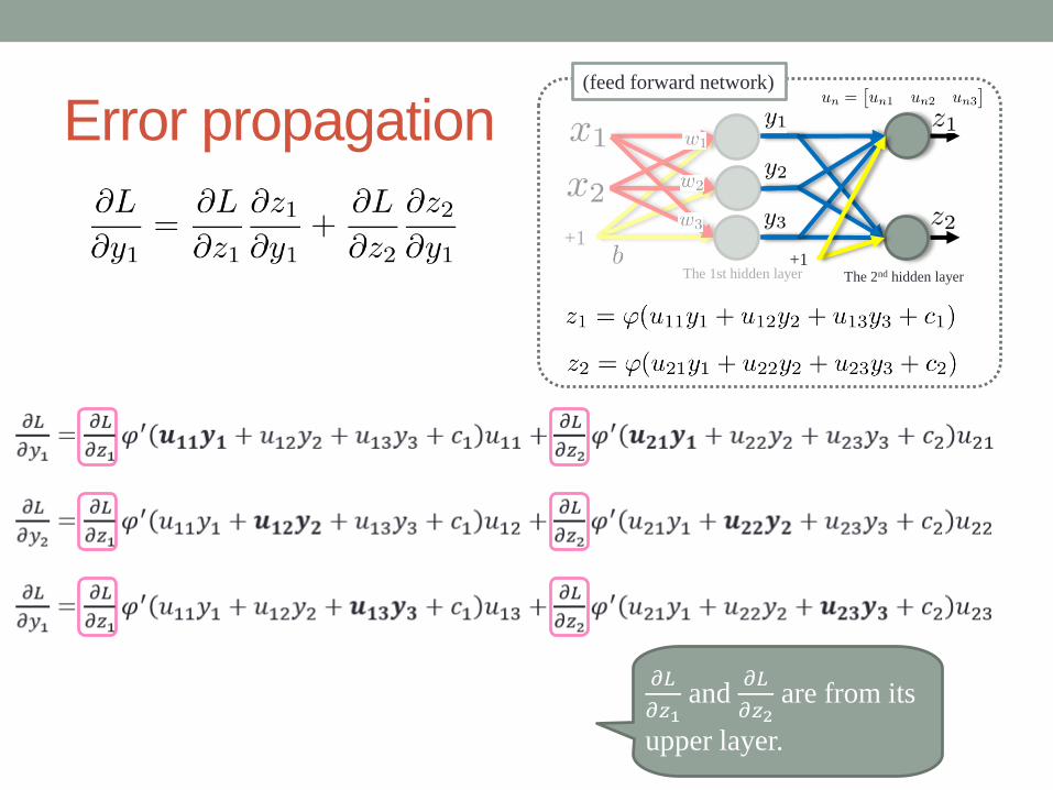
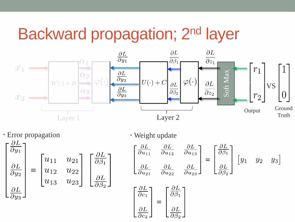
Error propagation(feed forward network)
The 2nd hidden layerThe 1st hidden layer
+1+1
𝜕𝐿
𝜕𝑧1and
𝜕𝐿
𝜕𝑧2are from its
upper layer.
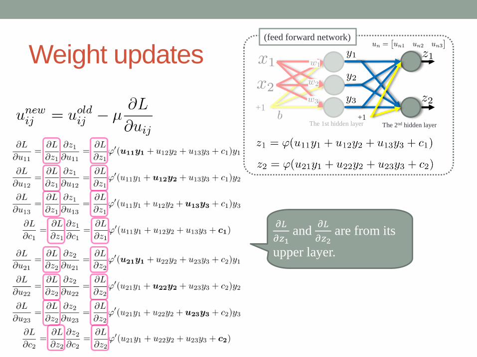
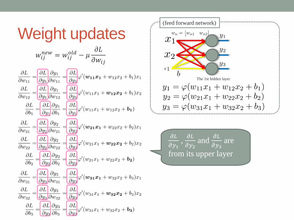
Weight updates(feed forward network)
The 2nd hidden layerThe 1st hidden layer
+1+1
𝜕𝐿
𝜕𝑧1and
𝜕𝐿
𝜕𝑧2are from its
upper layer.
Lay
er 1
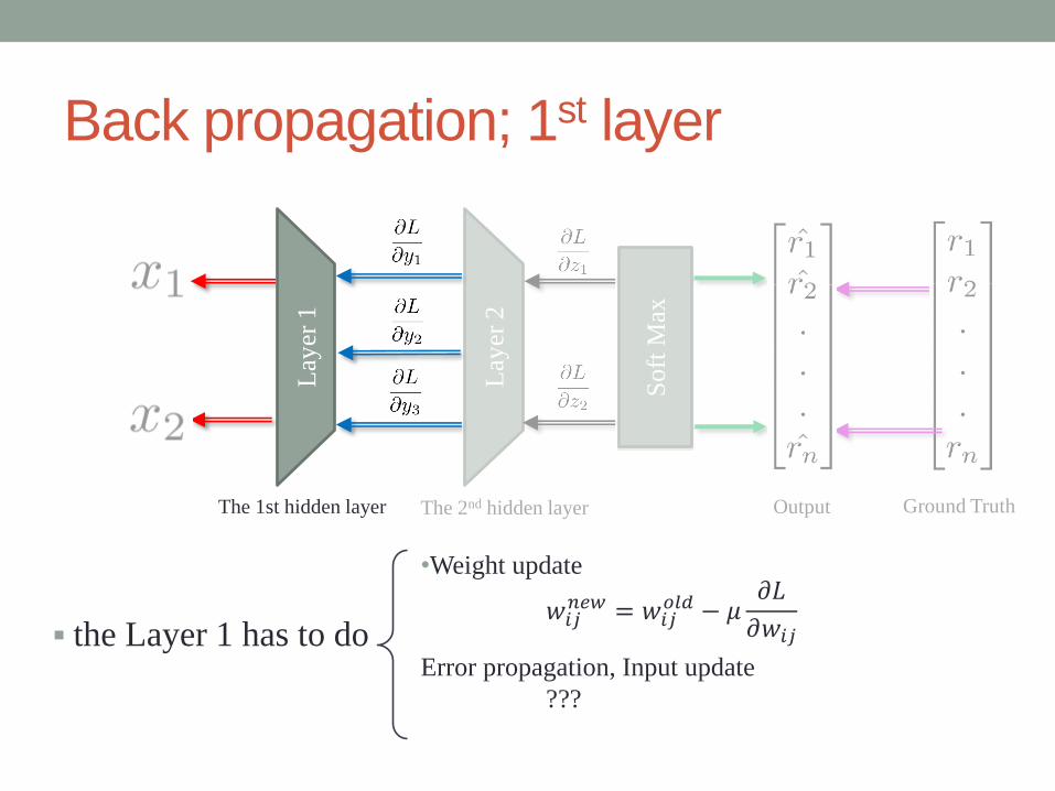
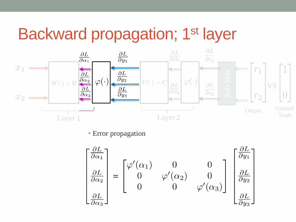
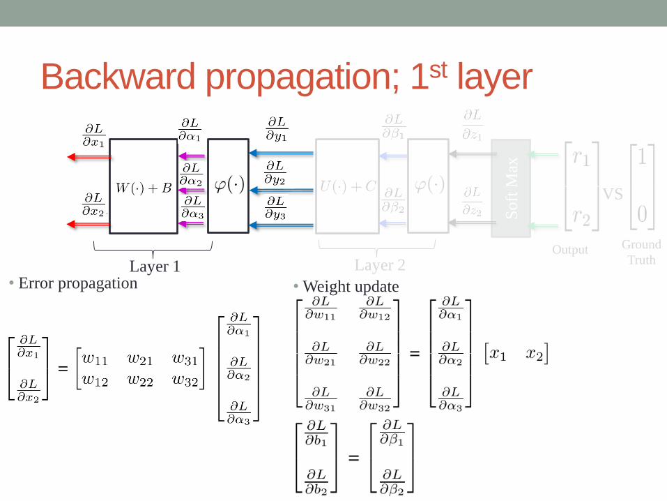
Back propagation; 1st layer
Lay
er 2
The 1st hidden layer The 2nd hidden layer
Soft
Max
Output Ground Truth
the Layer 1 has to do
•Weight update
Error propagation, Input update
???
𝑤𝑖𝑗𝑛𝑒𝑤 = 𝑤𝑖𝑗
𝑜𝑙𝑑 − 𝜇𝜕𝐿
𝜕𝑤𝑖𝑗
The 1st hidden layer
+1
(feed forward network)
Weight updates
𝜕𝐿
𝜕𝑦1, 𝜕𝐿
𝜕𝑦2and
𝜕𝐿
𝜕𝑦3are
from its upper layer
𝑤𝑖𝑗𝑛𝑒𝑤 = 𝑤𝑖𝑗
𝑜𝑙𝑑 − 𝜇𝜕𝐿
𝜕𝑤𝑖𝑗

Block-based perspective
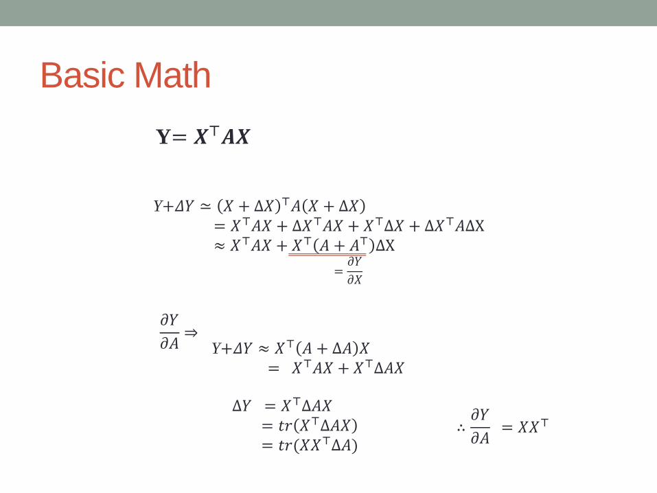
Basic Math
Y= 𝑿⊤𝑨𝑿
Y+𝛥𝑌 ≃ 𝑋 + Δ𝑋 ⊤𝐴 𝑋 + Δ𝑋= 𝑋⊤𝐴𝑋 + Δ𝑋⊤𝐴𝑋 + 𝑋⊤Δ𝑋 + Δ𝑋⊤𝐴ΔX≈ 𝑋⊤𝐴𝑋 + 𝑋⊤ 𝐴 + 𝐴⊤ ΔX
=𝜕𝑌
𝜕𝑋
𝜕𝑌
𝜕𝐴⇒
Y+𝛥𝑌 ≈ 𝑋⊤ 𝐴 + Δ𝐴 𝑋= 𝑋⊤𝐴𝑋 + 𝑋⊤Δ𝐴𝑋
Δ𝑌 = 𝑋⊤Δ𝐴𝑋= 𝑡𝑟 𝑋⊤Δ𝐴𝑋= 𝑡𝑟(𝑋𝑋⊤Δ𝐴)
∴𝜕𝑌
𝜕𝐴= 𝑋𝑋⊤
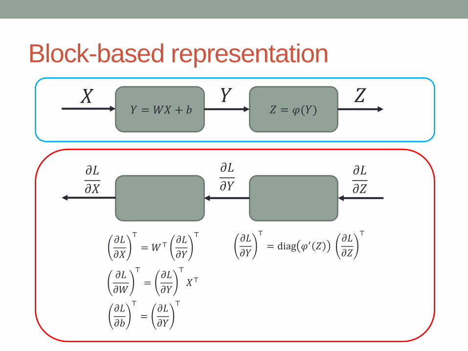
Block-based representation
𝑋 𝑌 𝑍𝑌 = 𝑊𝑋 + 𝑏 𝑍 = 𝜑(𝑌)
𝜕𝐿
𝜕𝑍
𝜕𝐿
𝜕𝑌𝜕𝐿
𝜕𝑋
𝜕𝐿
𝜕𝑋
⊤
= 𝑊⊤𝜕𝐿
𝜕𝑌
⊤ 𝜕𝐿
𝜕𝑌
⊤
= diag 𝜑′ 𝑍𝜕𝐿
𝜕𝑍
⊤
𝜕𝐿
𝜕𝑊
⊤
=𝜕𝐿
𝜕𝑌
⊤
𝑋⊤
𝜕𝐿
𝜕𝑏
⊤
=𝜕𝐿
𝜕𝑌
⊤
Forward propagation
(block-based representation)
Output
Soft
Max
Layer 1
Layer 1
Layer 2
Layer 2
Backward propagation; 2nd layer
Ground
Truth
VS
Output
Soft
Max
Layer 1 Layer 2
• Error propagation
Backward propagation; 2nd layer
VS
Ground
Truth
VS
Output
Soft
Max
Layer 1 Layer 2
• Error propagation
Backward propagation; 2nd layer
• Weight update• Error propagation
Ground
Truth
VS
Output
Soft
Max
Layer 1 Layer 2
Backward propagation; 1st layer
• Error propagation
Ground
Truth
VS
Output
Soft
Max
Layer 1 Layer 2
Backward propagation; 1st layer
• Error propagation
Ground
Truth
VS
Output
Soft
Max
Layer 1 Layer 2
• Weight update
Input Optimization while
fixing all weights
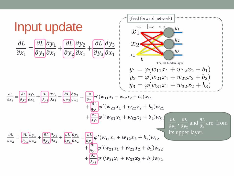
Input update
The 1st hidden layer
+1
(feed forward network)
𝜕𝐿
𝜕𝑦1, 𝜕𝐿
𝜕𝑦2and
𝜕𝐿
𝜕3are from
its upper layer.
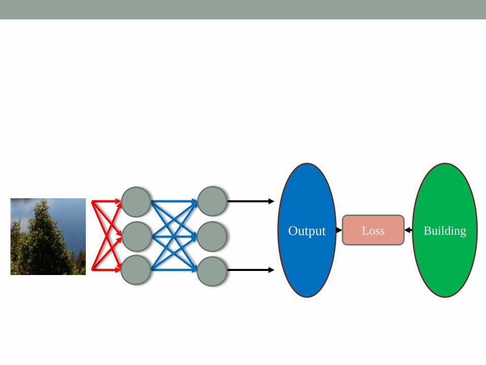
Output Loss Building
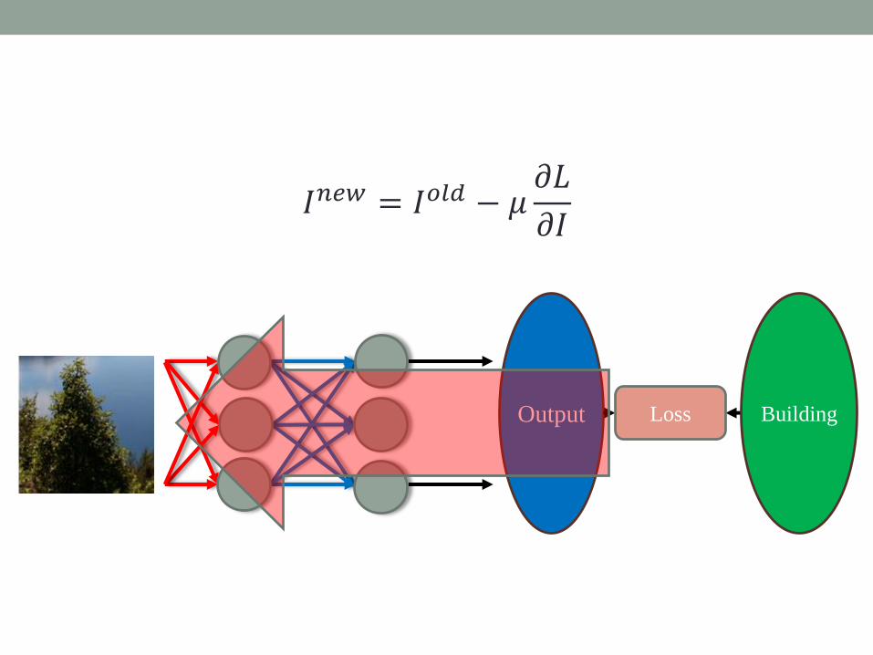
Output Loss Building
𝐼𝑛𝑒𝑤 = 𝐼𝑜𝑙𝑑 − 𝜇𝜕𝐿
𝜕𝐼

Output Loss Building
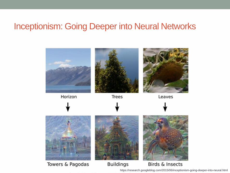
Inceptionism: Going Deeper into Neural Networks
https://research.googleblog.com/2015/06/inceptionism-going-deeper-into-neural.html
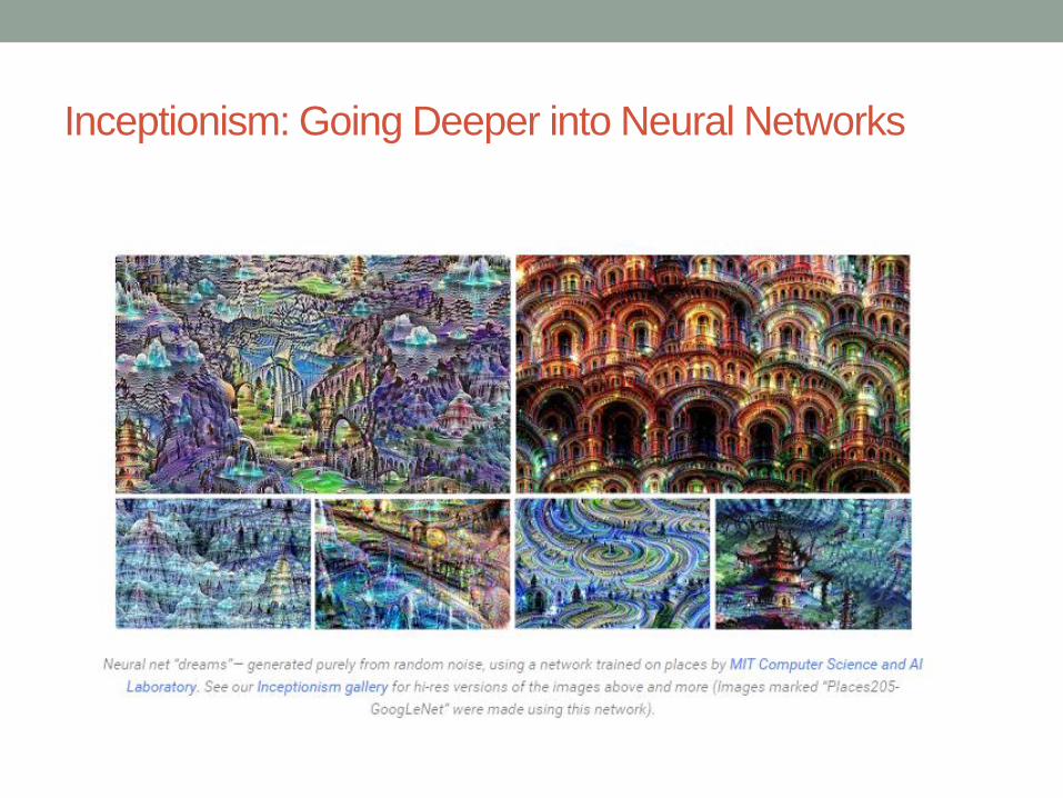
Inceptionism: Going Deeper into Neural Networks
DEEP INSIDE CONVOLUTION
NETWORKS
Inputs maximizing class score
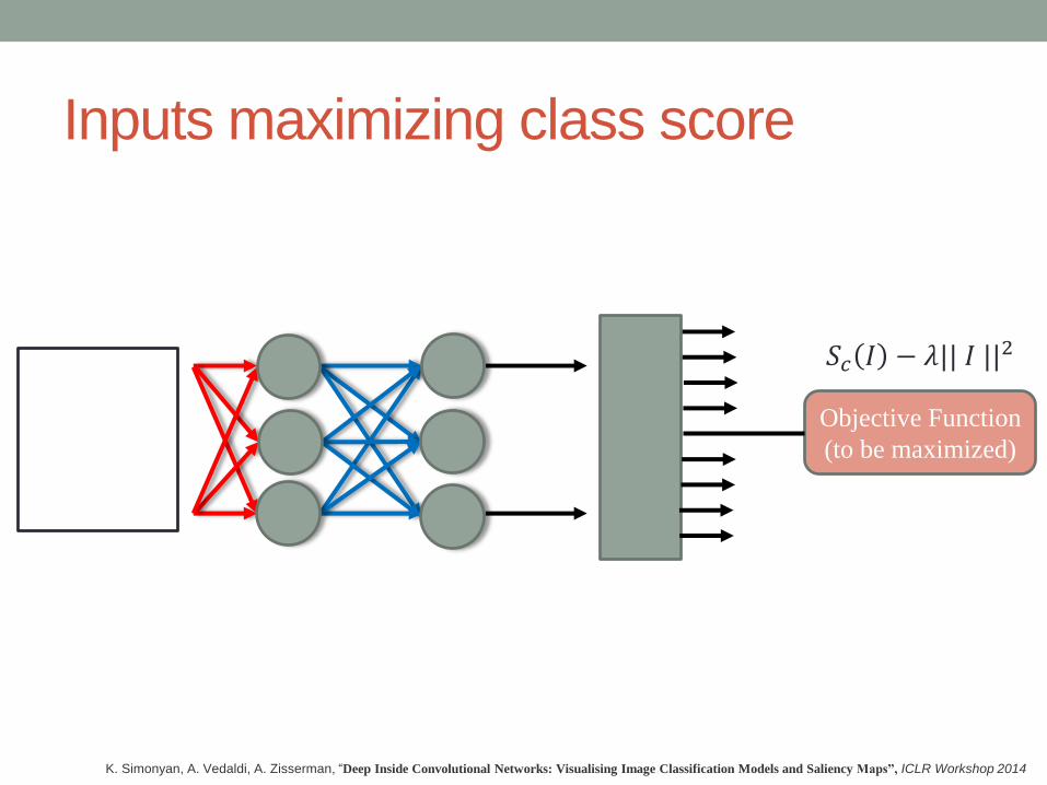
Inputs maximizing class score
Objective Function
(to be maximized)
K. Simonyan, A. Vedaldi, A. Zisserman, “Deep Inside Convolutional Networks: Visualising Image Classification Models and Saliency Maps”, ICLR Workshop 2014
𝑆𝑐 𝐼 − 𝜆|| 𝐼 ||2
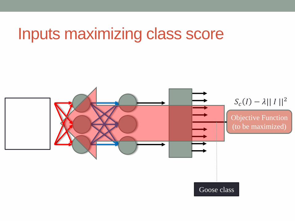
Inputs maximizing class score
Objective Function
(to be maximized)
Goose class
𝑆𝑐 𝐼 − 𝜆|| 𝐼 ||2
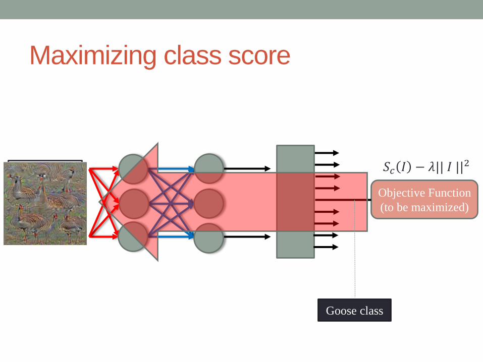
Maximizing class score
Objective Function
(to be maximized)
Goose class
𝑆𝑐 𝐼 − 𝜆|| 𝐼 ||2

Inputs maximizing class score
dumbbell
bell pepper
cup
lemon husky
dalmatian

Inputs maximizing class score
computer keyboard
Washing machine
kit fox
goose ostrich
limousine
DEEP INSIDE CONVOLUTION
NETWORKS
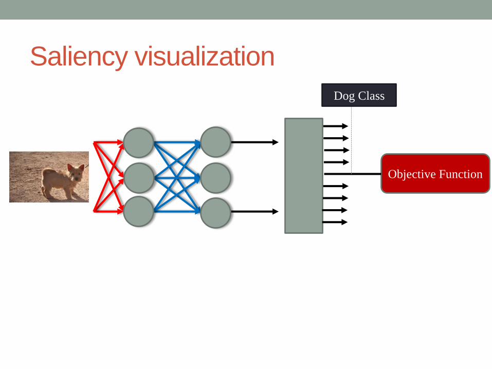
Saliency visualization
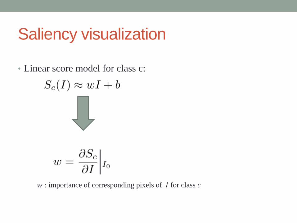
Saliency visualization
• Linear score model for class c:
𝑤 : importance of corresponding pixels of 𝐼 for class 𝑐
Saliency visualization
Objective Function
Dog Class
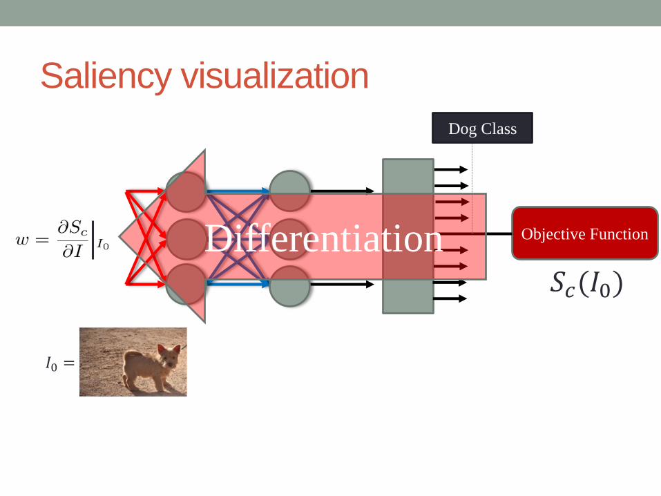
Saliency visualization
Objective Function
Dog Class
Differentiation
𝐼0 =
𝑆𝑐(𝐼0)
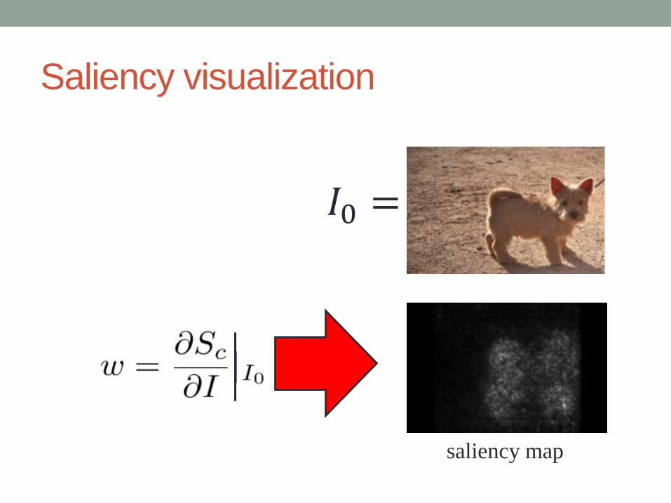
Saliency visualization
saliency map
𝐼0 =
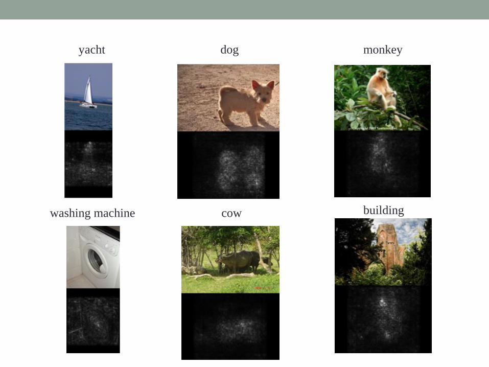
yacht dog monkey
buildingcowwashing machine
A NEURAL ALGORITHM OF
ARTISTIC STYLE

Loss
Gatys, Leon A., Alexander S. Ecker, and Matthias Bethge. "A neural algorithm of artistic style." arXiv preprint arXiv:1508.06576 (2015).
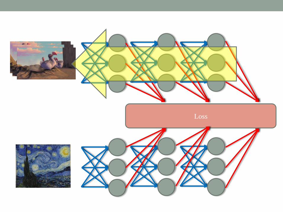
Loss
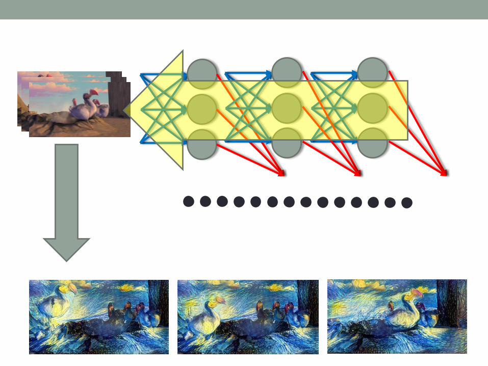

Artistic style
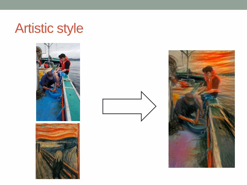
Artistic style

Backups
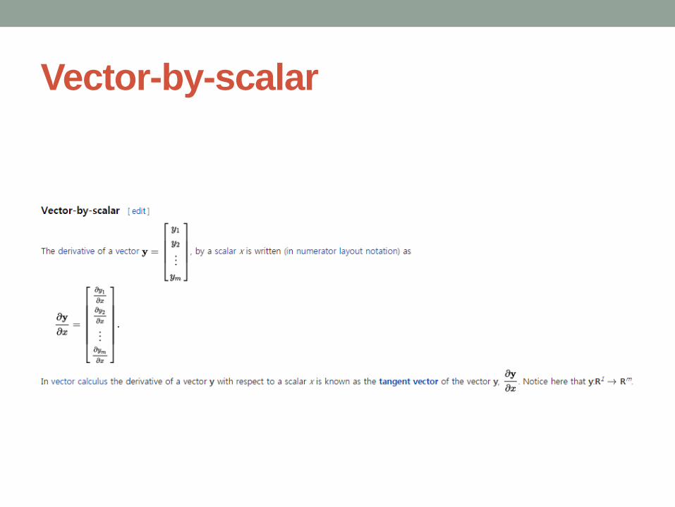
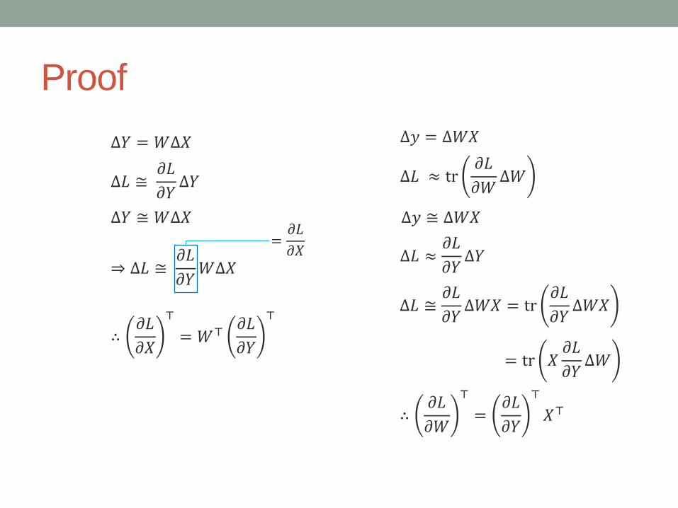
Vector-by-scalar
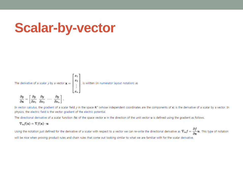
Scalar-by-vector
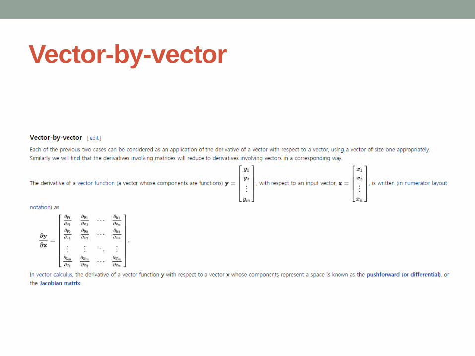
Vector-by-vector
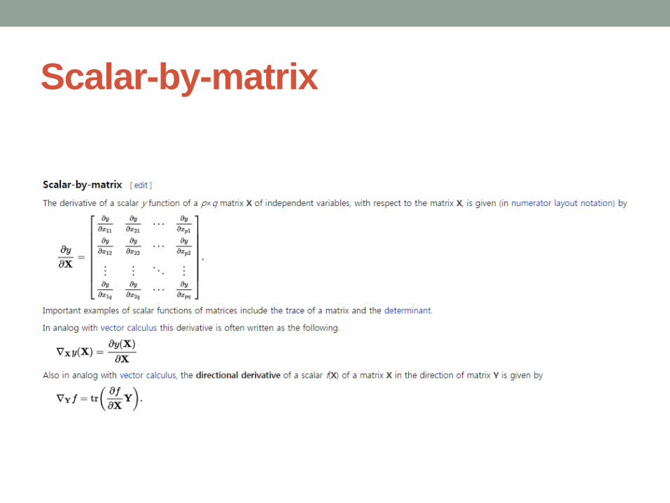
Scalar-by-matrix
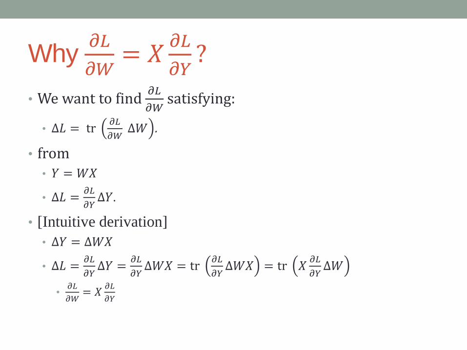
Why 𝜕𝐿
𝜕𝑊= 𝑋
𝜕𝐿
𝜕𝑌?
• We want to find 𝜕𝐿
𝜕𝑊satisfying:
• Δ𝐿 = tr𝜕𝐿
𝜕𝑊Δ𝑊 .
• from• 𝑌 = 𝑊𝑋
• Δ𝐿 =𝜕𝐿
𝜕𝑌Δ𝑌.
• [Intuitive derivation]
• Δ𝑌 = Δ𝑊𝑋
• Δ𝐿 =𝜕𝐿
𝜕𝑌Δ𝑌 =
𝜕𝐿
𝜕𝑌Δ𝑊𝑋 = tr
𝜕𝐿
𝜕𝑌Δ𝑊𝑋 = tr 𝑋
𝜕𝐿
𝜕𝑌Δ𝑊
•𝜕𝐿
𝜕𝑊= 𝑋
𝜕𝐿
𝜕𝑌
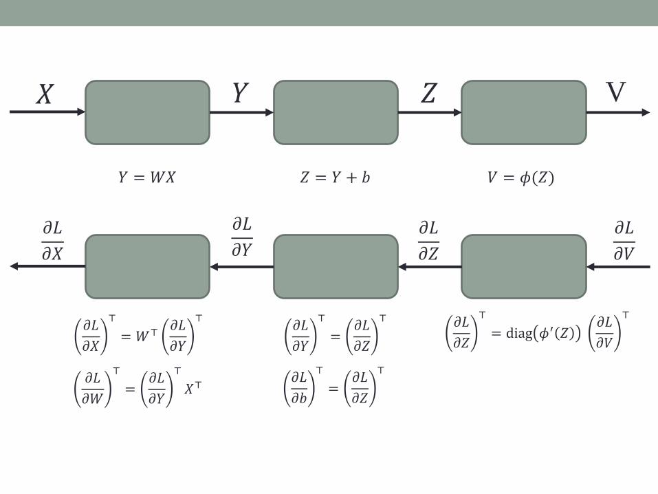
𝑋 𝑌 𝑍 V
𝑌 = 𝑊𝑋 𝑍 = 𝑌 + 𝑏 𝑉 = 𝜙(𝑍)
𝜕𝐿
𝜕𝑉
𝜕𝐿
𝜕𝑍
𝜕𝐿
𝜕𝑌𝜕𝐿
𝜕𝑋
𝜕𝐿
𝜕𝑋
⊤
= 𝑊⊤𝜕𝐿
𝜕𝑌
⊤𝜕𝐿
𝜕𝑌
⊤
=𝜕𝐿
𝜕𝑍
⊤ 𝜕𝐿
𝜕𝑍
⊤
= diag 𝜙′ 𝑍𝜕𝐿
𝜕𝑉
⊤
𝜕𝐿
𝜕𝑊
⊤
=𝜕𝐿
𝜕𝑌
⊤
𝑋⊤𝜕𝐿
𝜕𝑏
⊤
=𝜕𝐿
𝜕𝑍
⊤
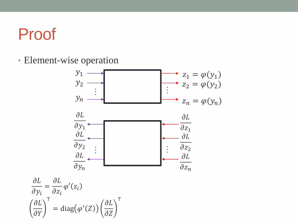
Proof
• Element-wise operation
…
𝑦1
…𝑦2
𝑦𝑛
𝑧1 = 𝜑(𝑦1)𝑧2 = 𝜑(𝑦2)
𝑧𝑛 = 𝜑(𝑦𝑛)
…
𝜕𝐿
𝜕𝑦1…
𝜕𝐿
𝜕𝑦2𝜕𝐿
𝜕𝑦𝑛
𝜕𝐿
𝜕𝑧1𝜕𝐿
𝜕𝑧2𝜕𝐿
𝜕𝑧𝑛
𝜕𝐿
𝜕𝑌
⊤
= diag 𝜑′ 𝑍𝜕𝐿
𝜕𝑍
⊤
𝜕𝐿
𝜕𝑦𝑖=
𝜕𝐿
𝜕𝑧𝑖𝜑′ 𝑧𝑖
⇒ ∆𝐿 ≅𝜕𝐿
𝜕𝑌𝑊∆𝑋
=𝜕𝐿
𝜕𝑋
Proof
∆𝐿 ≅𝜕𝐿
𝜕𝑌∆𝑌
∆𝑌 ≅ 𝑊∆𝑋
∴𝜕𝐿
𝜕𝑋
⊤
= 𝑊⊤𝜕𝐿
𝜕𝑌
⊤
∆𝑦 = ∆𝑊𝑋
∆𝐿 ≈ tr𝜕𝐿
𝜕𝑊∆𝑊
∆𝑦 ≅ ∆𝑊𝑋
∆𝐿 ≈𝜕𝐿
𝜕𝑌∆𝑌
∆𝐿 ≅𝜕𝐿
𝜕𝑌∆𝑊𝑋 = tr
𝜕𝐿
𝜕𝑌∆𝑊𝑋
= tr 𝑋𝜕𝐿
𝜕𝑌∆𝑊
∴𝜕𝐿
𝜕𝑊
⊤
=𝜕𝐿
𝜕𝑌
⊤
𝑋⊤
∆𝑌 = 𝑊∆𝑋

New Layer Design
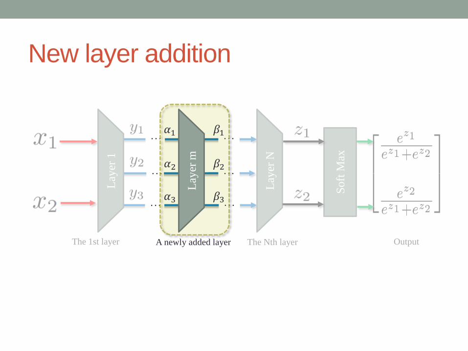
New layer addition
The 1st layer The Nth layer
So
ft M
ax
Lay
er 1
Lay
er N
OutputA newly added layer
…
…
…
…
…
…
𝛽1
𝛽3
𝛽2
Lay
er m
𝛼1
𝛼3
𝛼2
𝑑𝐿
𝑑𝛽3
𝑑𝐿
𝑑𝛽2
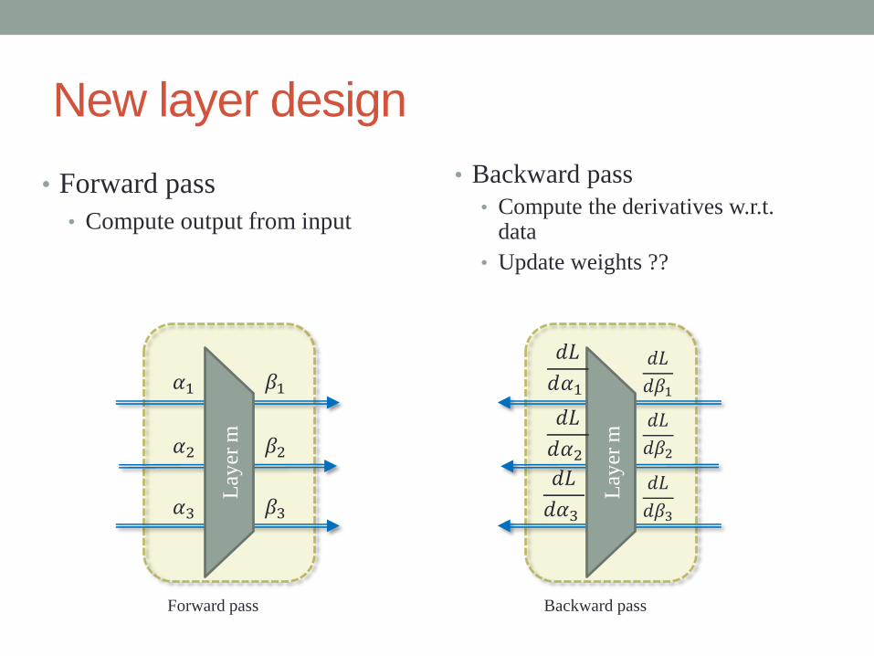
New layer design
• Forward pass
• Compute output from input
Backward pass
𝑑𝐿
𝑑𝛽1
Lay
er m
𝑑𝐿
𝑑𝛼3
𝑑𝐿
𝑑𝛼2
𝑑𝐿
𝑑𝛼1
Forward pass
Lay
er m
𝛽1
𝛽3
𝛽2
𝛼1
𝛼3
𝛼2
• Backward pass
• Compute the derivatives w.r.t. data
• Update weights ??

Max
pooli
ng
lay
er
Example: Max pooling
5 6 3 9
2 1 4 11
17 14 3 21
11 13 12 9
6 11
17 21

Derivatives of max
𝑑𝐿
𝑑𝑧
Backward passm
ax
𝑑𝐿
𝑑𝑥=𝑑𝐿
𝑑𝑧
𝑑𝑧
𝑑𝑥
Forward pass
max
x
y
z
• For forward pass • For backward pass
𝑑𝐿
𝑑y=𝑑𝐿
𝑑𝑧
𝑑𝑧
𝑑𝑦
![Analyzing Deep Neural Networks with Symbolic Propagation: … · 2021. 2. 22. · Analyzing Deep Neural Networks with Symbolic Propagation 297 Specifically, [29] discovers that it](https://static.documents.pub/doc/80x56/613d407a984e1626b6577850/analyzing-deep-neural-networks-with-symbolic-propagation-2021-2-22-analyzing.jpg)


