1 Neural Networks and Static Modelling Igor Belič Institute of Metals and Technology Slovenia 1. Introduction Neural networks are mainly used for two specific tasks. The first and most commonly mentioned one is pattern recognition and the second one is to generate an approximation to a function usually referred to as modelling. In the pattern recognition task the data is placed into one of the sets belonging to given classes. Static modelling by neural networks is dedicated to those systems that can be probed by a series of reasonably reproducible measurements. Another quite important detail that justifies the use of neural networks is the absence of suitable mathematical description of modelled problem. Neural networks are model-less approximators, meaning they are capable of modelling regardless of any knowledge of the nature of the modelled system. For classical approximation techniques, it is often necessary to know the basic mathematical model of the approximated problem. Least square approximation (regression models), for example, searches for the best fit of the given data to the known function which represents the model. Neural networks can be divided into dynamic and static neural (feedforward) networks, where the term dynamic means that the network is permanently adapting the functionality (i.e., it learns during the operation). The static neural networks adapt their properties in the so called learning or training process. Once adequately trained, the properties of the built model remain unchanged – static. Neural networks can be trained either according to already known examples, in which case this training is said to be supervised, or without knowing anything about the training set outcomes. In this case, the training is unsupervised. In this chapter we will focus strictly on the static (feedforward) neural networks with supervised training scheme. An important question is to decide which problems are best approached by implementation of neural networks as approximators. The most important property of neural networks is their ability to learn the model from the data presented. When the neural network builds the model, the dependences among the parameters are included in the model. It is important to know that neural networks are not a good choice when research on the underlying mechanisms and interdependencies of parameters of the system is being undertaken. In such cases, neural networks can provide almost no additional knowledge. www.intechopen.com
Transcript
1
Neural Networks and Static Modelling
Igor Belič Institute of Metals and Technology
Slovenia
1. Introduction
Neural networks are mainly used for two specific tasks. The first and most commonly mentioned one is pattern recognition and the second one is to generate an approximation to a function usually referred to as modelling.
In the pattern recognition task the data is placed into one of the sets belonging to given classes. Static modelling by neural networks is dedicated to those systems that can be probed by a series of reasonably reproducible measurements. Another quite important detail that justifies the use of neural networks is the absence of suitable mathematical description of modelled problem.
Neural networks are model-less approximators, meaning they are capable of modelling regardless of any knowledge of the nature of the modelled system. For classical approximation techniques, it is often necessary to know the basic mathematical model of the approximated problem. Least square approximation (regression models), for example, searches for the best fit of the given data to the known function which represents the model.
Neural networks can be divided into dynamic and static neural (feedforward) networks, where the term dynamic means that the network is permanently adapting the functionality (i.e., it learns during the operation). The static neural networks adapt their properties in the so called learning or training process. Once adequately trained, the properties of the built model remain unchanged – static.
Neural networks can be trained either according to already known examples, in which case this training is said to be supervised, or without knowing anything about the training set outcomes. In this case, the training is unsupervised.
In this chapter we will focus strictly on the static (feedforward) neural networks with supervised training scheme.
An important question is to decide which problems are best approached by implementation of neural networks as approximators. The most important property of neural networks is their ability to learn the model from the data presented. When the neural network builds the model, the dependences among the parameters are included in the model. It is important to know that neural networks are not a good choice when research on the underlying mechanisms and interdependencies of parameters of the system is being undertaken. In such cases, neural networks can provide almost no additional knowledge.
www.intechopen.com
Recurrent Neural Networks and Soft Computing
4
The first sub-chapter starts with an introduction to the terminology used for neural networks. The terminology is essential for adequate understanding of further reading.
The section entitled ”Some critical aspects” summarizes the basic understanding of the topic and shows some of the errors in formulations that are so often made.
The users who want to use neural network tools should be aware of the problems posed by the input and output limitations. These limitations are often the cause of bad modelling results. A detailed analysis of the neural network input and output considerations and the errors that may be produced by these procedures are given.
In practice the neural network modelling of systems that operate on a wide range of values represents a serious problem. Two methods are proposed for the approximation of wide range functions.
A very important topic of training stability follows. It defines the magnitude of diversity detected during the network training and the results are to be studied carefully in the course of any serious data modelling attempt.
At the end of the chapter the general design steps for a specific neural network modelling task are given .
2. Neural networks and static modelling
We are introducing the term of static modelling of systems. Static modelling is used to model the time independent properties of systems which implies that the systems behaviour remains relatively unchanged within the time frame important for the application. (Fig. 1). In this category we can understand also the systems which do change their reaction on stimulus, but this variability is measurable and relatively stable in the given time period. We regard the system as static when its reaction on stimulus is stable and most of all repeatable – in some sense - static.
The formal description of static system (Fig. 1) is given in (1)
Ym(Xn, t) = f (Xn, Pu, t) (1)
Where Ym is the m - dimensional output vector,
Xn is the n – dimensional input – stimulus vector, Pu is the system parameters vector, t is the time.
In order to regard the system as static both the function f and the parameters vector Pu do not change in time.
),,( tPXf unnX mY
Fig. 1. The formal description of static system.
www.intechopen.com
Neural Networks and Static Modelling
5
Under the formal concept of static system we can also imply a somewhat narrower definition as described in (1). Here the system input – output relationship does not include the time component (2).
Ym (Xn) = f(Xn, Pu) (2)
Although this kind of representation does not seem to be practical, it addresses a very large group of practical problems where the nonlinear characteristic of a modelled system is corrected and accounted for (various calibrations and re-calibrations of measurement systems).
Another understanding of static modelling refers to the relative speed (time constant) of the system compared to the model. Such is the case where the model formed by the neural network (or any other modelling technique) runs many times faster than does the original process which is corrected by the model1.
We are referring to the static modelling when the relation (3) holds true.
m << s (3)
Where m represents the time constant of the model, and s represents the time constant of the observed system. Due to the large difference in the time constants, the operation of the model can be regarded as instantaneous.
The main reason to introduce the neural networks to the static modelling is that we often do not know the function f (1,2) analytically but we have the chance to perform the direct or indirect measurements of the system performance. Measured points are the entry point to the neural network which builds the model through the process of learning.
3. The terminology
The basic building element of any neural network is an artificial neural network cell (Fig. 2 left).
(.)
x1
x2
x3
xn
Activation
function
Summing
junction
Synaptic
weights
Bias input
Inputs
wk1
wk2
wk3
wkn
wkb
Output
yk
Input
layer
Hidden
layers
Output
layer
OutputsInputs
1 2 n
. . .
. . .
. . .
. . .
. . .. . .
Fig. 2. The artificial neural network cell (left) and the general neural network system (right)
1The measurement systems usually (for example vacuum gauge) operate indirectly. Through measurement of different parameters the observed value of the system (output) can be deduced. Such is the case with the measurement of the cathode current at inverted magnetron. The current is in nonlinear dependence with the pressure in the vacuum system. In such system the dependence of the current versus pressure is not known analytically – at least not good enough - to use the analytical expression directly. This makes ideal ground to use neural network to build the adequate model.
www.intechopen.com
Recurrent Neural Networks and Soft Computing
6
Each artificial neural network consists of a number of inputs (synapses) that are connected to the summing junction. The values of inputs are multiplied by adequate weights w (synaptic weights) and summed with other inputs. The training process changes the values of connection weights, thus producing the effect of changing the input connection strengths. Sometimes there is a special input to the neural cell, called the bias input. The bias input value is fixed to 1, and the connection weight is adapted during the training process as well. The value of summed and weighted inputs is the argument of an activation function (Fig. 3) which produces the final output of an artificial neural cell. In most cases, the activation function ( )x is of sigmoidal2 type. Some neural network architectures use the mixture of
sigmoidal and linear activation functions (radial basis functions are a special type of neural network that use the neural network cells with linear activation functions in the output layer and non-sigmoidal functions in the hidden layer).
Artificial neural network cells are combined in the neural network architecture which is by default composed of two layers that provide communication with “outer world” (Fig. 2 right). Those layers are referred to as the input and output layer respectively. Between the two, there is a number of hidden layers which transform the signal from the input layer to the output layer. The hidden layers are called “hidden” for they are not directly connected, or visible, to the input or output of the neural network system. These hidden layers contribute significantly to the adaptive formation of the non-linear neural network input-output transfer function and thus to the properties of the system.
0 .0 0
0 .2 0
0 .4 0
0 .6 0
0 .8 0
1 .0 0
-5 -4 -3 -2 -1 0 1 2 3
x - S um o f ne ura l ne tw ork ce ll inpu ts
y -
ac
tiv
ati
on
φ (x) = y =
Satur at ion m arg in Sm = 0 .1 - in te rva l
0 -1 is lim ited to 0 .05 - 0.95
Fig. 3. The activation function ( )x of an artificial neural network cell.
2 One of the sigmoidal type functions is ( ) 1 /(1 )xx e .
www.intechopen.com
Neural Networks and Static Modelling
7
3.1 Creation of model – The training process
The process of adaptation of a neural network is called “training” or “learning”. During supervised training, the input – output pairs are presented to the neural network, and the training algorithm iteratively changes the weights of the neural network.
The measured data points are consecutively presented to the neural network. For each data point, the neural network produces an output value which normally differs from the target value. The difference between the two is the approximation error in the particular data point. The error is then propagated back through the neural network towards the input, and the correction of the connection weights is made to lower the output error. There are numerous methods for correction of the connection weight. The most frequently used algorithm is called the error backpropagation algorithm.
The training process continues from the first data point included in the training set to the very last, but the queue order is not important. A single training run on a complete training data set is called an epoch. Usually several epochs are needed to achieve the acceptable error (training error) for each data point. The number of epochs depends on various parameters but can easily reach numbers from 100,000 to several million.
When the training achieves the desired accuracy, it is stopped. At this point, the model can reproduce the given data points with a prescribed precision for all data points. It is good practice to make additional measurements (test data set) to validate the model in the points not included in the training set. The model produces another error called the test error, which is normally higher than the training error.
4. Some critical aspects
Tikk et al. (2003) and Mhaskar (1996) have provided a detailed survey on the evolution of approximation theory and the use of neural networks for approximation purposes. In both papers, the mathematical background is being provided, which has been used as the background for other researchers who studied the approximation properties of various neural networks.
There is another very important work provided by Wray and Green (1994). They showed that, when neural networks are operated on digital computers (which is true in the vast majority of cases), real limitations of numerical computing should also be considered. Approximation properties like universal approximation and the best approximation become useless.
The overview of mentioned surveys is given in (Belič, 2006).
The majority of works have frequently been used as a misleading promise, and even proof, that neural networks can be used as the general approximation tool for any kind of function. The provided proofs are theoretically correct but do not take into account the fact that all those neural network systems were run on digital computers.
Nonlinearity of the neural network cell simulated on a digital computer is realized by polynomial approximation. Therefore, each neural cell produces a polynomial activation function. Polynomial equivalence for the activation function is true even in the theoretical sense, i.e., the activation function is an analytical function, and analytical functions have their polynomial equivalents.
www.intechopen.com
Recurrent Neural Networks and Soft Computing
8
The output values of the neural network can be regarded as the sum of polynomials which is just another polynomial. The coefficients of the polynomial are changed through the adaptation of neural network weights. Due to the finite precision of the numeric calculations the contributions, of the coefficients with higher powers become lower from the finite precision of the computer. The process of training can no longer affect them. This is also true of any kind of a training scheme.
The work of Wray and Green (1994) has been criticized, but it nevertheless gives a very important perspective to the practitioners who cannot rely just on the proofs given for theoretically ideal circumstances.
There are many interesting papers describing the chaotic behaviour of neural networks (Bertels, et.al., 1996), (Huang, 2008), (Yuan, Yang, 2009), (Wang, et.al., 2011). The neural network training process is a typical chaotic process. For practical applications this fact must never be forgotten.
Neural networks can be used as a function approximation (modelling) tool, but they neither perform universal approximation, nor can the best approximation in a theoretical sense be found.
A huge amount of work has been done trying to find proofs that a neural network can provide approximation of continuous functions. It used to be of interest because the approximated function is also continuous and exists in a dense space. Then came the realization that, even if the approximated function is continuous, its approximation is not continuous since the neural network that performs the approximation consists of a finite number of building blocks. The approximation is therefore nowhere dense, and the function is no longer continuous. Although this does not sound promising, the discontinuity is not of such a type that it would make neural network systems unusable. This discontinuity must be understood in a numerical sense.
Another problem is that neural networks usually run on digital computers, which gives rise to another limitation mentioned earlier: as it is not always possible to achieve the prescribed approximation precision, the fact that neural networks can perform the approximation with any prescribed precision does not hold.
Furthermore, another complication is that continuity of the input function does not hold. When digital computers are used (or in fact any other measurement equipment), the denseness of a space and the continuity of the functions cannot be fulfilled for both input and output spaces. Moreover, when measurement equipment is used to probe the input and output spaces (real physical processes), denseness of a space in a mathematical sense is never achieved. For example, the proofs provided by Kurkova (1995) imply that the function to be approximated is in fact continuous, but the approximation process produces a discontinuous function. This is incorrect in practice where the original function can never be continuous in the first place.
A three layer neural network has been proved to be capable of producing a universal approximation. Although it is true (for the continuous functions), this is not practical when the number of neural cells must be very high, and the approximation speed becomes intolerably low. Introducing more hidden layers can significantly lower the number of neural network cells used, and the approximation speed then becomes much higher.
www.intechopen.com
Neural Networks and Static Modelling
9
Numerous authors have reported on their successful work regarding the neural networks as approximators of sampled functions. Readers are kindly requested to consult those reports and findings to name but a few (Aggelogiannaki, et.al. 2007), (Wena, Ma, 2008), (Caoa, et.al., 2008), (Ait Gougam, et.al., 2008), (Bahi, et.al., 2009), (Wanga, Xub, 2010).
4.1 Input and output limitations
Neural networks are used to model various processes. The measurements obtained on the system to be modelled are of quite different magnitudes. This represents a problem for the neural network where the only neural network output (and often input) range is limited to the [0,1] interval. This is the case since the neural network cell activation function ( )x (Fig.
3) saturates output values at values 0 and 1. The users should be well aware of the processes as these are often the cause of various unwanted errors.
For some neural network systems this range is expanded to the [-1,+1] interval.
This is the reason why the input and output values of the neural network need to be preconditioned. There are two basic procedures to fit the actual input signal to the limited interval to avoid the saturation effect. The first process is scaling, and the second is offsetting.
First, the whole training data set is scanned, and the maximal maxy and minimal
miny values are found. The difference between them is then the range which is to be scaled
to the [0-1] interval. From all values y the value of miny is subtracted (this process is called
offsetting). The transformation of the values is obtained by the equation
min
max min
' ii
y yy
y y
(4)
Here 'iy represents the offset and scaled value that fits in the prescribed interval. The
reverse transformation is obtained by the equation
min max min'i iy y y y y (5)
The process is exactly the same for the neural network input values, only the interval is not necessarily limited to the 0 – 1 values.
This is not the only conditioning that occurs on input and output sides of the neural network. In addition to scaling, there is a parameter that prevents saturation of the system and is called scaling margin. The sigmoidal function tends to become saturated for the big values of inputs (Fig. 3). If the proper action is to be assured for the large values as well, then the scaling should not be performed on the whole [0,1] interval. The interval should be smaller for the given amount (let us say 0.1 for 10% shrinking of the interval). The corrected values are now
min
max min
(1 )( )'
2m im
i
S y ySy
y y
(6)
www.intechopen.com
Recurrent Neural Networks and Soft Computing
10
where mS represents the scaling margin.
The reverse operation is obtained by the equation
max min
min
'2
1
mi
im
Sy y y
y yS
(7)
When selecting the value of 0.1mS , this means that the actual values are scaled to the
interval [0.05 , 0.95] (see Fig. 3).
The training process is usually stopped when the prescribed accuracy is achieved on the training data set. However, there is still an important issue to discuss in order to understand the details. The parameter “training tolerance” is user set, and it should be set according to the special features of each problem studied.
Setting the training tolerance to the desired value (e.g. 0.1) means that the training process will be stopped when, for all training samples, the output value does not differ from the target value by more than 10 % of the training set range. If the target values of the training set lie between 100 and 500, then setting the training tolerance parameter value to 0.1 means that the training process will stop when, for all values, the differences between the target and the approximated values will not differ by more than 40 ( 10% of 500-100). Formally this can be written with the inequality:
max min; Ti i Tfor all i y y y y (8)
Here Tiy represents the target value for the ith sample, iy is the modelled value for the ith
sample, T is the training tolerance, and maxy , miny are the highest and the lowest value of
the training set.
It is not common practice to define the tolerance with regard to the upper and lower values of the observation space. For the case when neural networks are used to approximate the unipolar functions, the absolute error dE is always smaller than the training tolerance
d TE (9)
The absolute error produced by the neural network approximation for the ith sample becomes:
max
Ti id
i
y yE
y
(10)
while the relative error is:
T
i iri T
i
y yE
y
(11)
www.intechopen.com
Neural Networks and Static Modelling
11
and the relation between the absolute and relative error is:
maxr di i T
i
yE E
y (12)
And furthermore
maxri T T
i
yE
y (13)
An important conclusion follows from the last inequality. At the values where Tiy is much
smaller than maxy , the relative error becomes very high, and, therefore, the results of the
modelling become useless for these small values. This implies that the span between maxy
and miny should not be too broad (depending on the particular problem but, if possible,
not higher then two decades), otherwise the modelling will result in a very poor
performance for the small values.
To avoid this problem other strategies should be used.
4.2 Approximation for wide range functions
The usual study of neural network systems does not include the use of neural networks in a wide range of input and output conditions.
As shown in the previous section, neural networks do not produce a good approximation when the function to be approximated spans over a wide range (several decades).
The quality of approximation (approximation error) of small values is very poor compared with that of large ones. The problem can be solved by means of:
a. Log/Anti Log Strategy; the common and usual practice is to take the measured points and to perform the logarithm (log10) function. The logartihmic data is then used as input and target values for the neural network; or
b. segmentation strategy; the general idea is to split the input and output space into several smaller segments and perform the neural network training of each segment separately. This also means that each segment is approximated by a separate neural network (sub network). This method not only gives much better approximation results, but it also requires a larger training set (at least 5 data points per segment). It is also a good practice to overlap segments in order to achieve good results on segment borders.
5. Training stability analysis
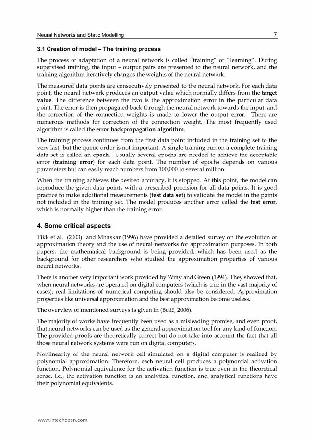
The training process of a neural network is the process which, if repeated, does not lead to equal results. Each training process starts with different, randomly chosen connection weights so the training starting point is always different. Several repetitions of the training process lead to different outcomes. Stability of the training process refers to a series of outcomes and the maximal and minimal values, i.e., the band that can be expected for the particular solution. The narrower the obtained band, the more stable approximations can be expected (Fig. 4).
www.intechopen.com
Recurrent Neural Networks and Soft Computing
12
The research work on the stability band has been conducted on 160 measured time profile samples. For each sample, 95 different neural network configurations have been systematically tested. Each test has included 100 repetitions of the training process, and each training process required several thousand epochs. From the vast database obtained, statistically firm conclusions can be drawn. So much of work was necessary to prove the importance of the stability band. In practice users need to perform only one or two tests to get the necessary information.
0.00
1.00
2.00
3.00
4.00
5.00
6.00
0.0 0 100. 00 200.0 0 300.00 400.00 500.00
tim e [min ]
pre
ssure
sta b ility ba n d u pp e r
bo u nd a ry
sta b ilit y b an d lo w er
b ou n da ry
Fig. 4. The different training processes produce different models. A possible outcome of an arbitrarily chosen training process falls within the maximal and minimal boundaries which define the training “stability band”.
The procedure for the determination of the training stability band is the following:
1. Perform the first training process based on the training data set and randomly chosen neural network weights.
2. Perform the modelling with the trained neural network in the data points between the training data points.
3. The result of the modelling is the first so-called reference model. This means that the model is used to approximate the unknown function in the space between the measured points. The number of approximated points should be large enough so the approximated function can be evaluated with sufficient density. Practically this means the number of approximated points should be at least 10 times larger than the number of measured data points (in the case presented, the ratio between the number of measured and the number of approximated points was 1:15).
4. Perform the new training process with another set of randomly chosen weights. 5. Compare the outcomes of the new model with the previous one and set the minimal
and maximal values for all approximated points. The first band is therefore obtained and bordered by the upper and lower boundaries.
www.intechopen.com
Neural Networks and Static Modelling
13
6. Perform the new training process with another set of randomly chosen weights. 7. For each approximated point perform the test to see whether it lies within the established
lower or upper boundary. If this is not the case, extend the particular boundary value. 8. Repeat steps 6, 7 and 8 until the prescribed number of repetitions is achieved.
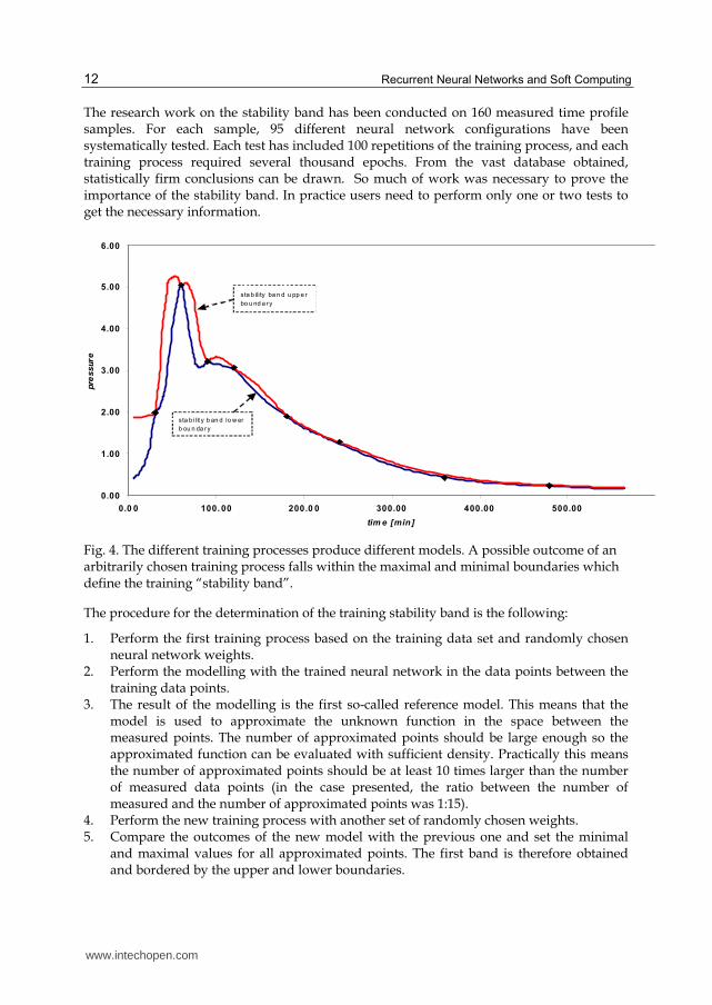
Fig. 5. The training stability upper boundary change vs. the number of separate training experiments. The training stability band does not change significantly after the 100th training experiment.
The practical question is how many times should the training with the different starting values for the connection weights, be performed to assure that the training stability band no longer changes in its upper and lower boundaries. Fig. 5 shows the stability band upper boundary changes for each separate training outcome (the distance from existing boundary and the new boundary). The results are as expected, and more separate trainings are performed, lesser the stability band changes. The recording of the lower boundary change gives very similar results. Fig. 5 shows clearly that the changes after the 100th repetition of training do not bring significant changes in the training stability band. In our further experiments the number of repetitions was therefore fixed to 100. When dealing with any new modelling problem, the number of required training repetitions should be assessed.
Only one single run of a training process is not enough because the obtained model shows only one possible solution, and nothing is really known about the behaviour of the particular neural network modelling in conjunction with the particular problem. In our work, the spinning rotor gauge error extraction modelling was performed and results were very promising (Šetina, et.al., 2006). However, the results could not be repeated. When the training stability test is performed, the range of possible solutions becomes known, and further evaluation of adequacy of the used neural network system is possible. The training stability band is used instead of the worst case approximation analysis. In the case where the complete training stability range is acceptable for the modelling purposes, any trained neural network can be used.
www.intechopen.com
Recurrent Neural Networks and Soft Computing
14
0.00
1.00
2.00
3.00
4.00
5.00
6.00
0.00 100.00 200.00 300.00 400.00 500.00
time[min]
pre
ss
ure
/err
or curve of ap proxim ate d
pressu re
stab ilit y ba nd wid th
Fig. 6. The upper curve represents the band centre line, which is the most probable model for the given data, and the lower curve represents the band width. The points depict the measured data points that were actually used for training. The lower curve represents the width of the training stability band. The band width is the smallest at the measured points used for training.
When the band is too wide, more emphasis has to be given to find the training process that gives the best modelling. In this case, genetic algorithms can be used to find the best solution (or any other kind of optimization) (Goldberg, 1998).
Following a very large number of performed experiments it was shown that the middle curve (centre line) (Fig. 6) between the maximal and minimal curve is the most probable curve for the observed modelling problem. The training stability band middle range curve can be used as the best approximation, and the training repetition that produces the model closest to the middle curve should be taken as best.
Some practitioners use the strategy of division of the measured points into two sets: one is used for training purposes and the other for the model evaluation purposes. This is a very straightforward strategy, but it works well only when the number of the measured points is large enough (in accordance with the dynamics of the system–sampling theorem). If this is not the case, all measured points should be used for the training purposes, and an analysis of the training stability should be performed.
6. The synthesis (design) of neural networks for modelling purposes
Neural network modelling is always based on the measurement points which describe the modelled system behaviour. It is well known from the information theory that the observed function should be sampled frequently enough in order to preserve the system information. Practically, this means that the data should be gathered at least 10 times faster than the highest frequency (in temporal or spatial sense) produced by the system (Shannon’s
www.intechopen.com
Neural Networks and Static Modelling
15
theorem). If the sampled data is too sparse, the results of the modelling (in fact any kind of modelling) will be poor, and the modelling tools can not be blamed for bad results.
The synthesis of a neural network should be performed in several steps:
1. Select the training data set which should be sampled adequately to represent the observed problem. Input as well as output (target) parameters should be defined.
2. Check the differences between the maximal and minimal values in the training set (for input and output values). If the differences are too high, the training set should be segmented (or logarithmed), and for each segment the separate neural network should be designed.
3. Set the first neural network which should consist of three layers (one being the hidden layer). Set the training tolerance parameter that satisfies the modelling needs. Choose an arbitrary number of neural cells in the hidden layer (let’s say 10) and start the training procedure. Observe the way in which the neural network performs the training. If the training process shows a steady decrease of the produced training error, the chosen number of neural cells in the hidden layer is sufficient to build the model. If the output error shows unstable behaviour and it does not decrease with the number of epochs then the number of cells in the hidden layer might be too small and should be increased. If the speed of the neural network output error decreases too slowly for practical needs, then another hidden layer should be introduced. It is interesting that the increase of number of neural cells in one hidden layer does not significantly improve the speed of training convergence. Only addition in a new hidden layer can lower the training convergence speed. Addition of too many hidden layers also can not guarantee better training convergence. There is a certain limit to a training convergence speed that can be reached with an optimal configuration, and it depends on the problem at hand.
4. Perform the training stability test and decide whether further optimization is needed. It is interesting that the training stability band mostly depends on the problem being modelled and that the various neural network configurations do not alter it significantly.
5. At step 4, the design of the neural network is completed and it can be applied to model the problem
Usually, one of the modelled parameters is time. In this case, one of the inputs represents the time points when the data samples were taken. Fig. 6 shows the model of degassing a vacuum system where the x axis represents the time in minutes and the y axis represents the total pressure in the vacuum system (in relative numerical values). In this case, the only input to the neural network was time and the target was to predict the pressure in the vacuum chamber.
7. The example of neural network modelling
Suppose we are to model a bakeout process in a vacuum chamber. The presented example should be intended for industrial circumstances, where one and the same production process is repeated in the vacuum chamber. Prior to the production process, the entire system must be degassed using an appropriate regime depending on the materials used. The model of degassing will be used only to monitor the eventual departure of the vacuum
www.intechopen.com
Recurrent Neural Networks and Soft Computing
16
chamber pressure temporal profile. Any difference in the manufacturing process as it is the introduction of different cleaning procedures might result in a different degassing profile. A departure from the usual degassing profile should result in a warning signal indicating possible problems in further production stages.
For the sake of simplicity, only two parameters will be observed, time t and pressure in the vacuum chamber p. Practically, it would be appropriate to monitor temperature, heater current, and eventual critical components of mass spectra as well.
First, it has to be determined which parameters are primary and which are their consequences. In the degassing problem, one of the basic parameters is the heater current, another being time. As a consequence of the heater current, the temperature in the vacuum chamber rises, the degassing process produces the increase of pressure and possible emergence of critical gasses etc. Therefore, the time and the heater current represent the input parameters for the neural network, while parameters such as temperature, pressure, and partial pressures are those to be modelled.
In the simplified model, we suppose that, during the bakeout process, the heater current always remains constant and is only switched on at the start and off after the bakeout. We also suppose that there is no need to model mass spectra and temperature. Therefore, there are two parameters to be modelled, time as the primary parameter and pressure as the consequence (of constant heater current and time).
Since the model will be built for the industrial use, its only purpose is to detect possible anomalies in the bakeout stage. The vacuum chamber is used to process the same type of objects, and no major changes are expected to happen in the vacuum system as well. Therefore, the bakeout process is supposed to be repeatable to some extent.
Several measurements are to be made resulting in the values gathered in Table 1..
Time [min] Numeric values of pressure
30 0.51
60 0.95
90 0.96
120 1.40
180 2.40
240 2.13
360 1.00
480 0.56
600 0.30
Table 1. Measurements of bakeout of the vacuum system. The time–pressure pairs are the training set for the neural network.
The model is built solely on the data gathered by the measurements on the system. As mentioned before, neural networks do not need any further information on the modelled system.
www.intechopen.com
Neural Networks and Static Modelling
17
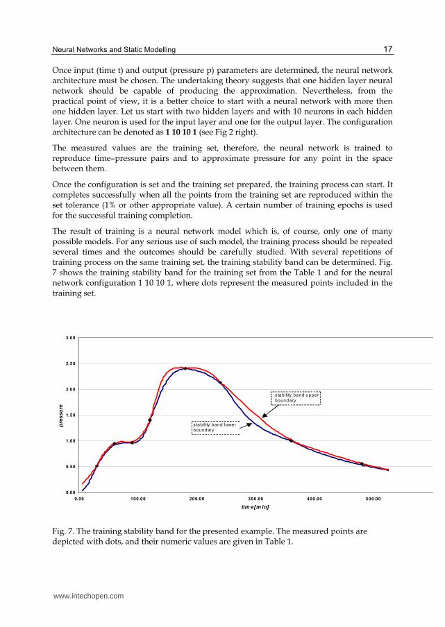
Once input (time t) and output (pressure p) parameters are determined, the neural network architecture must be chosen. The undertaking theory suggests that one hidden layer neural network should be capable of producing the approximation. Nevertheless, from the practical point of view, it is a better choice to start with a neural network with more then one hidden layer. Let us start with two hidden layers and with 10 neurons in each hidden layer. One neuron is used for the input layer and one for the output layer. The configuration architecture can be denoted as 1 10 10 1 (see Fig 2 right).
The measured values are the training set, therefore, the neural network is trained to reproduce time–pressure pairs and to approximate pressure for any point in the space between them.
Once the configuration is set and the training set prepared, the training process can start. It completes successfully when all the points from the training set are reproduced within the set tolerance (1% or other appropriate value). A certain number of training epochs is used for the successful training completion.
The result of training is a neural network model which is, of course, only one of many possible models. For any serious use of such model, the training process should be repeated several times and the outcomes should be carefully studied. With several repetitions of training process on the same training set, the training stability band can be determined. Fig. 7 shows the training stability band for the training set from the Table 1 and for the neural network configuration 1 10 10 1, where dots represent the measured points included in the training set.
0.00
0.50
1.00
1.50
2.00
2.50
3.00
0.00 100.00 200.00 300.00 400.00 500.00
tim e[m in]
pre
ssu
re
s tability band upper
boundary
stability band lower
boundary
Fig. 7. The training stability band for the presented example. The measured points are depicted with dots, and their numeric values are given in Table 1.
www.intechopen.com
Recurrent Neural Networks and Soft Computing
18
If the training stability band is narrow enough, there is no real need to proceed with further optimisation of the model, otherwise the search for optimal or, at least, a sufficient model should continue.
It is interesting to observe the width of the training stability band for different neural network configurations. Fig. 8 provides the results of such study for the training set from the Table 1. It is important to notice that the diagram on Fig. 8 shows the average stability band-width for each neural network configuration. Compared to the values of the measured dependence, the average widths are relatively small, which is not always the case for maximal values of a training stability band. It would be more appropriate for certain problems to observe the maximal value of training stability band width instead of the average values.
On the other hand, the width of the training stability band is only one parameter to be observed. From the practical point of view, it is also important to know how time consuming the training procedure for different configurations really is. Fig. 9 provides some insights into this detail of neural network modelling. Even a brief comparison of Fig. 8 and Fig. 9 clearly shows that neural networks that enable a quick training process are not necessary those which also provide the narrowest training stability band.
0
0.002
0.004
0.006
0.008
0.01
0.012
0.014
0.016
0.018
1 5
15
20
1
1 1
0 1
5 2
0 1
1 5
10
1
1 5
10
15
11
15
20
15
1
1 5
20
20
1
1 1
5 1
5 1
5 1
1 1
0 1
5 1
5 1
1 5
15
15
1
1 5
10
20
1
1 5
10
10
1
1 5
20
15
1
1 1
0 2
0 2
0 1
1 5
15
10
1
1 2
0 2
0 1
5 1
1 2
0 2
0 2
0 1
1 5
15
1
1 1
0 1
5 1
1 2
0 1
5 1
0 1
1 1
5 1
5 1
0 1
1 1
5 1
5 2
0 1
1 1
5 1
0 2
0 1
1 2
0 2
0 1
0 1
1 1
5 2
0 2
0 1
1 5
20
1
1 1
0 1
5 1
0 1
1 1
5 2
0 1
0 1
1 1
0 2
0 1
5 1
1 2
0 1
5 1
5 1
1 1
0 2
0 1
1 2
0 1
0 1
1 1
5 1
5 1
1 2
0 1
0 1
5 1
1 1
0 1
0 1
0 1
1 1
5 5
20
1
1 2
0 1
0 5
1
1 1
0 2
0 1
0 1
1 1
0 1
5 5
1
1 5
5 1
0 1
1 1
0 1
0 2
0 1
1 5
5 1
5 1
1 1
5 1
0 1
0 1
1 5
5 2
0 1
1 1
0 5
20
1
1 1
5 1
0 1
1 2
0 1
5 2
0 1
1 1
0 1
0 1
1 2
0 1
0 2
0 1
1 1
0 1
0 1
5 1
1 1
5 1
0 1
5 1
1 5
5 1
1 2
0 5
1
1 1
5 5
1
1 1
5 2
0 1
1 5
15
5 1
1 5
10
5 1
1 1
5 5
5 1
1 2
0 1
0 1
0 1
1 5
5 5
1
1 2
0 2
0 5
11
10
5 1
0 1
1 5
20
5 1
1 1
0 5
5 1
1 2
0 1
5 1
1 1
0 1
0 5
11
20
5 1
0 1
1 1
5 1
0 5
1
1 2
0 2
0 1
1 2
0 1
5 5
11
15
15
51
NN co nfigu ra tion
av
era
ge
sta
bil
ity
ba
nd
wid
th
Fig. 8. Dependence of the average width of the training stability band versus the neural network configuration.
www.intechopen.com
Neural Networks and Static Modelling
19
0
50000
100000
150000
200000
250000
1 2
0 2
0 1
5 1
1 2
0 2
0 2
0 1
1 2
0 1
5 1
5 1
1 2
0 1
5 2
0 1
1 1
5 1
5 2
0 1
1 2
0 2
0 1
0 1
1 1
5 2
0 2
0 1
1 2
0 1
5 1
0 1
1 2
0 1
0 1
0 1
1 1
5 2
0 1
5 1
1 1
5 1
5 1
5 1
1 1
5 1
0 1
0 1
1 2
0 1
0 1
5 1
1 2
0 1
0 2
0 1
1 1
5 1
0 1
5 1
1 1
5 2
0 1
0 1
1 1
5 1
5 1
0 1
1 1
5 1
0 2
0 1
1 1
0 1
0 1
5 1
1 1
0 2
0 2
0 1
1 1
0 1
5 1
5 1
1 2
0 1
0 5
1
1 1
0 1
5 2
0 1
1 1
0 1
0 2
0 1
1 1
0 2
0 1
5 1
1 1
0 1
5 1
0 1
1 2
0 2
0 5
1
1 5
20
20
11
20
15
5 1
1 1
5 1
0 5
1
1 1
0 1
0 1
0 1
1 2
0 1
5 1
1 2
0 2
0 1
1 1
0 2
0 1
0 1
1 1
5 2
0 1
1 1
5 1
5 1
1 5
15
15
1
1 2
0 5
15
11
10
10
5 1
1 1
0 5
5 1
1 5
20
15
11
5 1
5 2
0 1
1 1
0 2
0 1
1 1
0 5
15
11
15
5 1
5 1
1 1
5 1
5 5
1
1 1
5 5
20
1
1 2
0 1
0 1
1 1
5 5
10
1
1 1
5 2
0 5
11
10
15
1
1 5
10
20
1
1 5
5 2
0 1
1 2
0 5
5 1
1 2
0 5
10
1
1 2
0 5
20
1
1 1
0 5
10
1
1 5
10
15
1
1 5
15
1
1 5
20
11
5 5
10
1
1 1
5 1
0 1
1 1
5 5
5 1
1 5
10
10
1
1 5
20
10
1
1 5
10
11
10
15
5 1
1 5
5 1
5 1
1 1
0 1
0 1
15
15
101
N N c on figura t io n
av
era
ge
nr.
of
ep
oc
hs
Fig. 9. Dependence of the average number of epochs versus the neural network configuration. The higher number of epochs needed usually means faster.
Fig. 10 is a representation of two properties: the average number of epochs (x axis), and the average training stability band width (y axis). Each point in the graph represents one neural network configuration. Interesting configurations are specially marked. It is interesting that the configuration with only one hidden layer performs very poorly. Even an increased number of neurons in the neural network with only one hidden layer does not improve the situation significantly.
If we seek for the configuration that will provide best results for the given trainig data set, we will try to provide the configuration that trains quickly (low number of epochs) and features the lowest possible training stability band width. Such configurations are 1 20 20 20 1 and 1 15 20 15 1. If we need the lowest possible training stability band-width then we will choose the configuration 1 5 15 20 1.
www.intechopen.com
Recurrent Neural Networks and Soft Computing
20
0
0 .0 0 2
0 .0 0 4
0 .0 0 6
0 .0 0 8
0.0 1
0 .0 1 2
0 .0 1 4
0 .0 1 6
0 .0 1 8
0 5 0 00 0 1 00 0 0 0 15 0 0 00 2
a ve ra ge nu m be r of e po ch s
av
era
ge s
tab
ilit
y b
an
d w
idth
1 1 5 20 1 5 1
1 20 2 0 20 1
1 40 1
1 5 15 2 0 1
1 2 0 5 5 1
Fig. 10. The optimisation process seeks the neural network that uses both the lowest possible number of epochs while producing an approximation with the narrowest training stability band. Each dot on the graph represents one neural network configuration. Interesting configurations are highlighted.
8. Conclusions
The field of neural networks as a tool for approximation (modelling) is very rapidly evolving. Numerous authors have reported their research results on the topic.
In this chapter, two very important issues of the theory of approximation are questioned. One is the universality of approximation, and the second is the best approximation property. Both properties are not applicable to the neural networks that run on digital computers.
Theoretically, it has been proven that a three layer neural network can approximate any kind of function. Although this is theoretically true, it is not a practical situation since the number of epochs needed to reach the prescribed approximation precision drops significantly with the increase in the number of hidden layers.
The newly introduced concept of approximation of wide-range functions by using logarithmic or segmented values gives the possibility to use neural networks as approximators in special cases where the modelled function has values spanning over several decades.
The training stability analysis is a tool for assessment of training diversity of neural networks. It gives information on the possible outcomes of the training process. It also provides the ground for further optimization.
www.intechopen.com
Neural Networks and Static Modelling
21
The important conclusions from the presented example are that the nature of the modelled problem dictates which neural network configuration performs the most appropriate approximation, and that, for each data set to be modelled, a separate neural network training performance analysis should be performed.
9. References
Aggelogiannaki, E., Sarimveis, H., Koubogiannis, D. (2007). Model predictive temperaturecontrol in long ducts by means of a neural network approximation tool. Applied Thermal Engineering. 27 pp 2363–2369
Ait Gougam, L., Tribeche, M. , Mekideche-Chafa, F. (2008). A systematic investigation of a neural network for function approximation. Neural Networks. 21 pp 1311-1317
Bahi, J.M., Contassot-Vivier , S., Sauget, M. (2009). An incremental learning algorithm for function approximation. Advances in Engineering Software. 40 pp 725–730
Belič, I. (2006). Neural networks and modelling in vacuum science. Vacuum. Vol. 80, pp 1107-1122
Bertels, K, Neuberg, L., Vassiliadis, S., Pechanek, D.G. (1998). Chaos and neural network learning – Some observations. Neural Process. Lett. 7, pp 69-80
Caoa, F., Xiea, T., Xub, Z.(2008). The estimate for approximation error of neural networks: A constructive approach. Neurocomputing . 71 pp 626–630
Goldberg, D.E. (1998). Genetic Algorithms in Search, Optimization, and Machine Learning. Addison-Wesley
Huang, W.Z., Huang, Y. (2008). Chaos of a new class of Hopfield neural networks. Applied
Mathematics and Computation. 206, (1) pp 1-11 Kurkova, V. (1995). Approximation of functions by perceptron networks with bounded
number of hidden units. Neural Networks. 8 (5), pp 745-750 Mhaskar, H.N. (1996). Neural Networks and Approximation Theory. Neural Networks, 9, (4),
pp 721-722 Šetina, J., Belič, I. (2006). Neural-network modeling of a spinning-rotor-gauge zero
correction under varying ambient temperature conditions. In: JVC 11, 11th Joint
Vacuum Conference, September 24 - 28, 2006, Prague, Czech Republic. Programme and book of abstracts, pp 99-100
Tikk, D., Kóczy, L.T., Gedeon, T.D. (2003). A survey on universal approximation and its limits in soft computing techniques. International Journal of Approximate Reasoning. 33(2), pp 185-202
Yuan, Q., Li, Q., Yang, X.S. (2009). Horseshoe chaos in a class of simple Hopfield neural networks. Chaos, Solitons and Fractals 39 pp 1522–1529
Wang, J., Xub, Z. (2010). New study on neural networks: The essential order of approximation. Neural Networks. 23 pp 618-624
Wang, T., Wang, K., Jia, N. (2011). Chaos control and associative memory of a time-delay globally coupled neural network using symmetric map. Neurocomputing 74 pp 1673–1680
Wena, C., Ma, X. (2008). A max-piecewise-linear neural network for function approximation. Neurocomputing . 71 pp 843–852
www.intechopen.com
Recurrent Neural Networks and Soft Computing
22
Wray, J., Green, G.G.R. (1994). Neural Networks, Approximation Theory and Finite Precision Computing. Neural Networks. 8 (1)
www.intechopen.com
Recurrent Neural Networks and Soft ComputingEdited by Dr. Mahmoud ElHefnawi
ISBN 978-953-51-0409-4Hard cover, 290 pagesPublisher InTechPublished online 30, March, 2012Published in print edition March, 2012