Neural Networks for Optimal Selection of The PID ...

IJCCCE, Vol.6, No.2, 2006

Control and Systems Eng. Dept. University of Technology, Baghdad. 92

Neural Networks for Optimal Selection of The PID Parameters and Designing Feedforward Controller

Mr. Ahmed S. Al-Araji & Miss May N. Bunny

Received on :21/12/2005 Accepted on :4/5/2006

Abstract A neural network-based feedforward controller and self-tuning PID controller

with optimization algorithm is presented. The scheme of the controller is based on two unknown models that describe the system and optimization algorithm. These models are modified Elman recurrent neural network and NARMA-L2. The modified Elman recurrent neural network (MERNN) model and NARMA-L2 model are learned with two stages off-line and on-line, in order to guarantee that the output of the model accurately represents the actual output of the system. The aim from the NARMA-L2 model is to find the Inverse Feedforward Controller (IFC) which controls the steady-state output of the system. The MERNN model after being learned is called the identifier. The feedback PID self tuning control signal for N-step ahead can be calculated the PID parameters by using the optimization algorithm with the quadratic performance index which is quadratic in the error between the desired set point and the model output, as well as quadratic of the control action. The paper explains the algorithm for a general case, and then a specific application on non-linear dynamical plant is presented.

الخلاصةو (Feedforward Neural Controller)أن الشبكة العصبیة أساس المسیطر التغـذیـة الأمامـیة

.لیة قدمت في ھذا البحثاذات التنغیم التلقائي مع الخوارزمیة المث PIDالمسیطرھذان أن ھیكلیة المسیطر المستخدم تتألف من نموذجین غیر معرفین یصفان المنظومة مع خوارزمیة المثلى

. (Modified Elman Neural Network & NARMA-L2)ن ھما یالنموذجلكي یضمن أن إخراج النموذج یمثل ألا خراج الحقیقي (On-line & Off-line)بمرحلتین أن نموذجین یتعلماً

Inverse)ھو أیجاد معكوس مسیطر التغذیة الأمامیة (NARMA-L2)أن الھدف من النموذج .وبصورة دقیقةFeedforward Controller) و الذي یتحكم بالاستجابة النھائیة للمنظومة.

(Identifier)" المعرف"الناتج بعد التعلم (Modified Elman Neural Network)ویطلق على النموذج ومن ثم یمكن حساب إشارة PIDومن المعرف و الخوارزمیة المثلیة یمكن حساب القیم المثلى للعناصر المسیطر

حقھ ولكل لحظھ من اجل السیطرة على الاستجابة العابرة للمنظومة اللا من الخطوات) ن (لتغذیة العكسیة لعدد اعن طریق تقلیل معامل الأداء وھو مربع الفرق بین ألا خراج المرغوب واخراج النموذج إضافة إلى مربع إشارة

.خطيلاوتم شرح ھذه الخوارزمیة واخذ مثال ذات تصرف . السیطرة

IJCCCE, Vol.6, No.2, 2006 Neural Networks for Optimal Selection of The PID Parameters and Designing Feedforward Controller

93

1- Introduction The application of intelligent

techniques to control systems has been a matter of wide study in recent years. These methods are used to solve complex problems that, in many cases, do not have an analytical solution. Neural networks (NNs), due to their ability to learn, have become a powerful tool in the development of the control systems. In fact nowadays, a new branch in control theory has arisen: Neuro control. This discipline studies the design of control systems aided by NN. Although in the process industry simple conventional controllers such as the PID have largely been extended, and show good performance for many tasks, when the plant or the process under control is complex or has high non-linearities. The control performance degrades notably [1]. This section gives a general overview of using neural networks in control systems and describes briefly a number of applications in this field. The neural network model can be used in control strategies that require a global model of the system forward or inverse dynamics, and these models are available in the form of neural networks, which have been trained using neural based system identification techniques. Papers by: Narandra andParthasarathy [2,3], Levin and Narandra [4] are some of those that can be referred to as the application of neural networks for system identification. Also Noriega & Wang [5] for general unknown nonlinear systems present a neural-network-based direct adaptive control strategy in the paper where a simplified formulation of the control signals is obtained of a feedforward neural network and an optimization scheme. The reason of study by the researchers is motivated by simplicity to implement the PID control in the industrial environment, by easiness of utilization by engineers and

process operators, and by acceptance in the industrial sector [6]. Some approaches proposed in the literature for deriving PID controllers are using self-tuning control techniques based on recursive parameter estimation, others are using automatic control techniques, and others are using intelligent control techniques. Despite the huge development in control theory, the majority of industrial processes are controlled by the well-established proportional-integral-derivative (PID) control. The popularity of PID control can be attributed to its simplicity and to its good performance in a wide range of operating conditions. In the last decade years, significant development has been established in the process control area to adjust the PID controller parameters automatically, in order to ensure adequate servo and regulatory behavior for a closed-loop plant [7,8,9] The organization of the paper is as follows: Section two describes the use of feedforward neural networks to learn to act as input-output model. Two models (modified Elman recurrent and NARMA-L2) for system identification is examined with the corresponding neural nets and learning mechanism used for this purpose. Section three represents the core of the present paper, and it is suggested using a feedforward neural controller and a feedback self tuning PID controller with optimization algorithm that will attain specific benefits towards a systematic engineering design procedure for neural control system. Illustrative example, that clarify the features of the proposed strategy are given in section four, where an example is discussed in detail. Finally, section five contains the conclusions of the entire work. 2- Identification of Dynamical Systems Using Neural Network Modeling


94

This section focuses on nonlinear system identification using two models of multi-layered feedforward neural network, the first one is modified Elman recurrent model and the second is NARMA-L2 model. The neural network is trained using Dynamic Back-Propagation Algorithm. A feedforward neural network can be seen as a system transforming a set of input patterns into a set of output patterns, and such a network can be trained to provide a desired response to a given input. The network achieves such a behavior by adapting its weights during the learning phase on the basis of some learning rules. 2-1 Recurrent Neural Networks

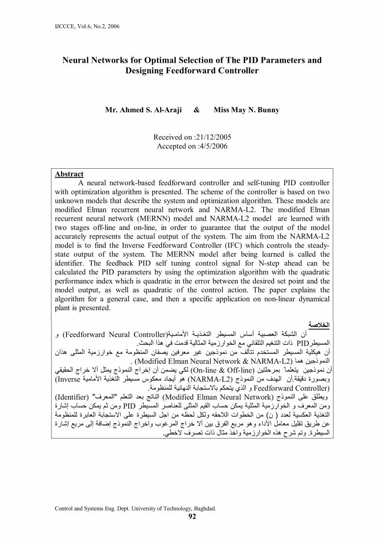
The Recurrent neural networks RNN structures are suitable to channel equalization and multi-user detection applications, since they are able to cope with channel transfer functions that exhibit deep spectral nulls, forming optimal decision boundaries and are less computationally demanding than MLP networks for these applications [10]. Among the available recurrent networks, modified Elman networks as shown in Fig (1) is one of the simplest types that can be trained using dynamic BP algorithm and it used to minimize the oscillation or even instabilities to the training controller. The output of the context unit in the modified Elman network is given by:

)1()1()( khkhkh coc

oc

(1) where )(khoc and )(khc are respectively the output of the context unit and hidden unit and is the feedback gain of the self-connections and is the connection weight from the hidden units (c’th)to the context units (c’th) at the context layer. The value of and are selected

randomly between (0 and 1). From the figure (1) it can be seen that the following equations:

)}(2),(1{)( khVkUVFkh o (2) )()( kWhkO (3)

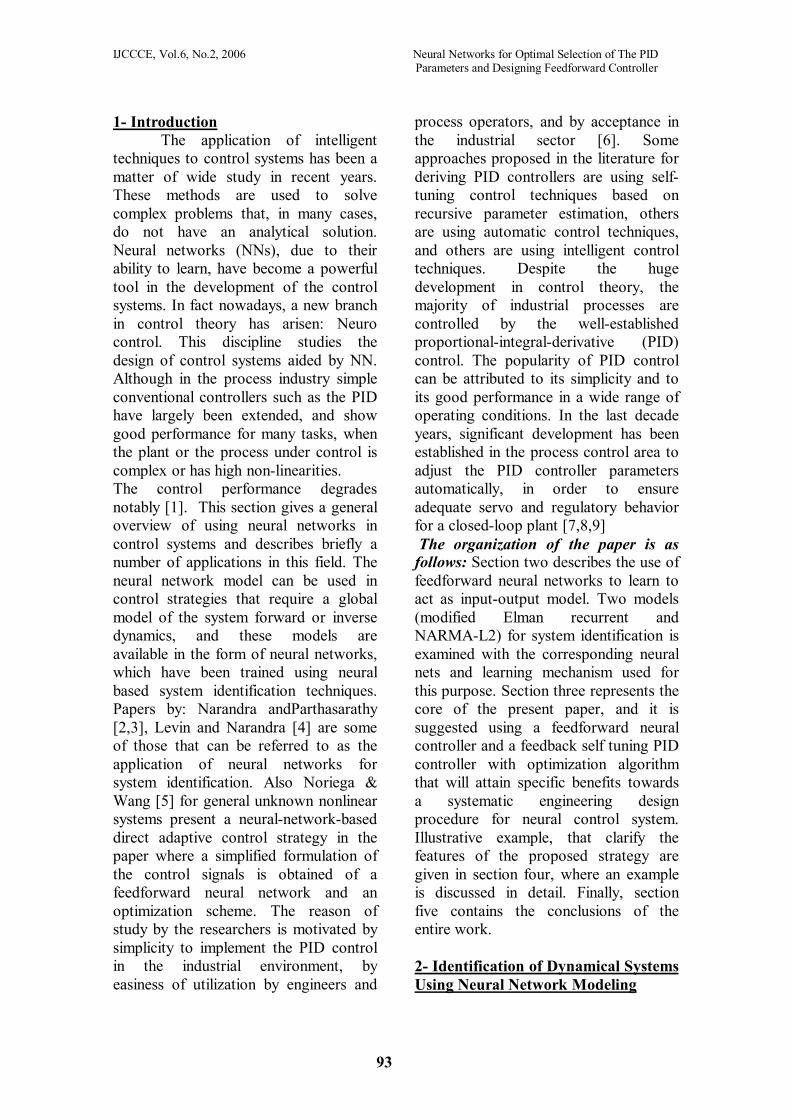
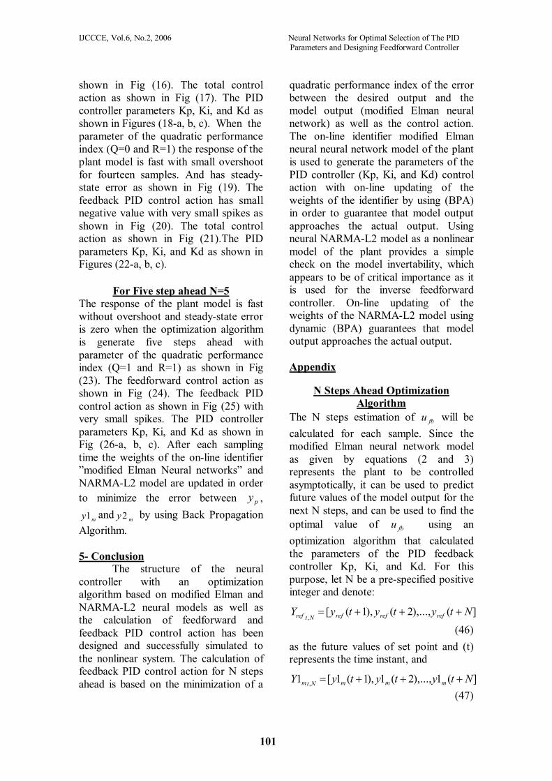
where V1,V2 and W are weight matrices and F is a non-linear vector function. The multi-layered modified Elman neural networks shown in figure (1) that is composed of many interconnected processing units called neurons or nodes. where: V 1: Weight matrix of the hidden layers. V 2: Weight matrix of the context layers. W : Weight matrix of the output layer. L : Denotes linear node. H : Denotes nonlinear node with sigmoidal function. To explain these calculations, consider the general j’th neuron in the hidden layer shown in figure (2). The inputs to this neuron consist of an ni – dimensional vector and (ni is the number of the input nodes). Each of the inputs has a weight V1 and V2 associated with it. The first calculation within the neuron consists of calculating the weighted sum

jnet of the inputs as [11]:

C

c

occj

nh

iiijj hVUVnet

1,

1, 21

(4) Where j=c. nh=C number of the hidden nodes and context nodes. Next the output of the neuron jh is calculated as the continuous sigmoid function of the jnet as:

jh = H( jnet ) (5)

H( jnet )= 11

2

jnete (6)


95

Once the outputs of the hidden layer are calculated, they are passed to the output layer. In the output layer, a single linear neuron is used to calculate the weighted sum (neto) of its inputs (the output of the hidden layer as in equation (7)).

neto k =

nh

jjkj hW

1

(7)

Where kjW is the weight between the hidden neuron jh and the output neuron. The single linear neuron, then, passes the sum (neto k ) through a linear function of slope 1 (another slope can be used to scale the output) as: )( kk netoLO , Where L (x)=x (8) The learning (training) algorithm is usually based on the minimization (with respect to the network weights) of the following objective cost function as equation (9).

np

i

np

i

im

ip

i kykykeE1 1

22 ))1(1)1((21))1((

21

(9) where np is number of patterns, ie is the error of each step, i

py is the actual output

of the plant of each step and imy1 is the

model output of the plant of each step. 2-2 NARMA-L2 Model Identification

Narendra and Mukhopadhyay in their paper [12] proposed two approximation input-output models (referred to by Narendra as NARMA-L1 and NARMA-L2) derived from the NARMA model, in which the control input appears linearly. The NARMA-L2 model requires only two neural networks to approximate the function f and g.

)]1nk(u),...,1k(u),1nk(y),...,k(y[f)1k(y ppp

)k(u)]1nk(u),...,1k(u),1nk(y),...k(y[g pp

(10)

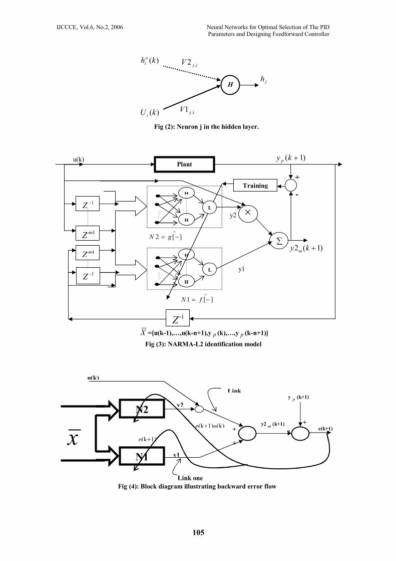
The identification model of NARMA-L2 model can be better illustrated as Fig (3), where X is represents the input vector of the networks N1 and N2 (the argument

of ][f

and ][g

). The same cost function in equation (9), is used for the learning algorithm that is usually based on the minimizing (with respect to the network weights) of the objective function.

np

i

np

i

im

ip

i kykykeE1 1

22 ))1(2)1((21))1((

21

(11) From Fig (3), it is important to note that the error between the desired output and the estimated neural network output needed to apply a supervised learning algorithm which is not available at the output N1 and N2. Hence, a little modification must be done to fit the algorithm to our case. This can be simply done by back-propagating the error at the output of the NARMA-L2 model (between y p (k+1) and y2 m (k+1)) to the output of N2 after multiplying it by u(k) and to the output of N1 directly. Figure (4) illustrates the error back-propagation and one can think of u(k) as a weight at link2. 3- The Controller Design

The control of nonlinear plants is considered in this section. The approach used to control the plant depends on the information available about the plant and the control objectives. The information of the unknown nonlinear plant can be known by the input-output data only and the plant is considered as (modified Elman networks model and NARMA-L2). The first step in the procedure of the control structure is the identification of the plant from the input-output data, and then a feedforward neural controller is used as the inverse of the plant. Also a feedback PID self tuning controller is


96

used based on the minimization of a quadratic performance index function of the error between the desired input and the actual output plant and of the feedback PID controller itself. An optimization algorithm is used to determine the control signal for N-steps ahead which will minimize the cost function in order to achieve good tracking of the reference signal and to use minimum effort. The integrated control structure that consists of the inverse of the plant, feedback self-tuning PID controller with an optimization algorithm and the series model reference, thus brings together the advantages of the inverse method with the robustness of feedback. The general structure of the neural controller can be given in the form of the block diagram shown in Fig (5). In the following sections, each part of the proposed controller will be explained in detail. 3-1 Feedforward Neural Controller (FFNC)

The feedforward neural controller is very important in the structure of the controller, because of its necessity to keep the steady-state tracking error to zero. This means that the action of the (FFNC) )k(u ff is to put the output of the plant as the reference input in steady state. Hence the (FFNC) is supposed to learn the inverse dynamic of the plant and so it is called inverse feedforward controller (IFC). To achieve this a neural using NARMA-L2 model equation (10) as explained in section two uses network for identification of the plant. When identification of the plant is complete then g[-] can be approximated by ][g

and f[-] by ][f

and the

NARMA-L2 model of the plant can be described by equation (12) below:

)]1nk(u),...,1k(u),1nk(y),...,k(y[f)1k(y ffffppm

)k(u)]1nk(u),...,1k(u),1nk(y),...,k(y[g ffffffpp

(12)

Likewise if ][g

is sign definite in the operating region then the network can be used as the inverse of the plant as given by equation (13).

)]1nk(u),...,1k(u),1nk(y),...,k(y[g

)]1nk(u),...1k(u),1nk(y),...,k(y[f)1k(y)k(u

ffffpp

ffffpprefff

(13) The sign definiteness of ][g

in the operating region (the region of interest) ensures the uniqueness of the plant inverse at that operating region [12]. Now by using equation (12) as the model of the plant identifier and equation (13) as the inverse mapping of the model, then these form the feedforward neural controller. The training of the inverse dynamic is done off-line and on-line. After the neural network has learned the inverse dynamic then )k(u ff is the control action required to keep the output of the plant at the reference value at steady state, hence it will be called equivalently as refu . 3-2 Feedback Self-Tuning Controller (PID)

The feedback self-tuning PID controller is also important because it is necessary to stabilize the tracking error dynamics of the system when the output of the plant is drifted from the input reference. The feedback PID controller consists of an on-line neural identifier and an optimization algorithm. The goal is to find the feedback control action that minimizes the cumulative error between the reference input and the output of the plant as well as a weighted sum of the control signal. This can be achieved by minimizing the following quadratic performance index [13].


97

N

1k

2ref

2pref ))k(u)k(u(R))1k(y)1k(y(Q

21J

(14) )k(uref is the reference control action and

it is equivalent to )k(u ff . )k(u is the total control signal

= )k(u ff + )k(ufb )k(ufb is the feedback control action.

)1k(y ref is the reference input. (Q, R) are positive weighting factors N is number of steps ahead Hence:

)k(u ref = )k(u ff (15) )k(u)k(u ff + )k(u fb (16)

Substituting equation (15) and (16) in (14) then J will be given:

N

1k

2fbffff

2pref )))k(u)k(u()k(u(R))1k(y)1k(y(Q

21

J

(17)

N

1k

2fb

2pref ))k(u(R))1k(y)1k(y(Q

21J

(18) This quadratic cost function will not only force the output to follow the reference input by minimizing the cumulative error N steps ahead but also forces the control action in the transient period to be as close as possible to the reference control signal. Also J depends on (Q and R) which are positive weighting factors. Hence the control action found will be optimal with respect to the given set of values of the weighting factors Q and R [13 &14]. The on-line identifier of the plant is to be used to obtain the predicted values of the output of the plant N steps ahead instead of running the plant itself N steps. These values are needed to calculate the feedback PID control action from the parameters Kp, Ki and Kd by the optimization algorithm such that the quadratic performance index J will be minimized. Also on line identification is required to make y1 m (k) the output of

the identifier as close as possible to the plant output y p (k). A feedforward neural network will be used as an identifier and two stages of learning of this neural network will be performed. The first stage is an off-line identification and the second stage is an on-line modification of the weights of the obtained identifier to keep track of any possible variation of the plant parameters. Therefore it can be said )()(1 kyky pm , and the performance index of equation (18) can be put as:

N

kfbmref kuRkykyQJ

1

22 ))(())1(1)1((21

(19)

N

1k

2fb

2 ))k(u(R))1k(e(Q21J

(20) )1(1)1()1( kykyke mref

(21) In this work a one hidden layer feedforward neural network is used for the identifier, hence

)()()1(11

1 netoLbiasWhWLkynh

jnhjjm

(22) The single linear neuron, then, passes the sum (neto) through a linear function of slope (1). Where the activation function of the hidden layer is a sigmoidal function and the output layer is a linear function [15]. Dynamic back propagation algorithm (BPA) is used to adjust the weights of the MERNN to learn the dynamics of the plant, and a simple gradient decent rule is used. After the identifier learns the dynamics of the system then the whole structure of the controller as shown in Fig (5) will be implemented. 3-3 The Series Model Reference

The model reference is used to overcome the harmonics of the step change in the set point desired and to


98

reduce the spikes of the control action of the feedforward neural controller [13 and 16]. Therefore the transient time of the plant is reduced and the overshoot is decreased. The model reference in the structure of the controller may be chosen as the difference equation (23):

)()1()1()1( kykyky refdesref (23) And is the tuning parameter. To ensure that the model reference is stable and to avoid ringing, the tuning parameter should be chosen as

10 [16 and 17]. Algorithm description of one step ahead control action

In this section, the feedback PID control signal )1( ku fb will be derived for one-step ahead depended on the parameters of the PID controller, that is when N=1. Where:

e(k)-1)1)[e(kKp(k(k)u1)(ku fbfb 1)e(k 1)Ki(k

1)]-e(k2e(k)-1)1)[e(kKd(k (24) Where Kp, Ki, and Kd denote the PID gains.

)()()1( kKpkKpkKp (25)

)()()1( kKikKikKi (26)

)()()1( kKdkKdkKd (27)

)()(

kKpJkKp

(28)

But:

])(

))((21

)(

))1((21

[)(

22

kKp

kuR

kKp

keQ

kKpJ fb

(29) Where:

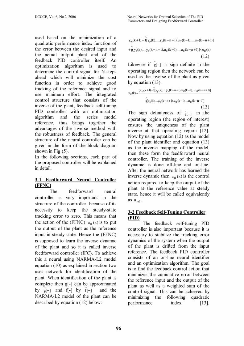
)1(1)1()1( kykyke mref (30) By the chain rule of differentiation we have

)()1(1

)1(1))1((

)())1(( 22

kKpky

kyke

kKpke m

m

)(

)1()1(2

kKpky

ke m

(31) And

)()1()())(( 2

kekekKpku fb

(32) Hence equation (29) becomes

)]()1(()(

)1(1)1([

)(kekeR

kKpky

kQekKpJ m

(33) For the two-layer modified Elman on-line neural network identifier shown in Fig (1) we have:

)()(

)()1(1

kKpneto

netonetoL

kKpky m

(34) For linear activation function output

1neto

)neto(L

)(1

)()1(1

kKph

hneto

kKpky j

j

m

(35)

)(1

)()1(1

1 kKpnet

neth

WkKpky j

j

jnh

jj

m

(36)

Where )net(H)h(121

neth

j2

jj

j


99

)()(

)()(1

)()1(1

1 kKpku

kunet

netHWkKpky j

j

nh

jj

m

(37)

)())()((

)(1)(

)1(1

1 kKpkuku

VnetHWkKpky fbff

jij

nh

jj

m

(38)

)]()1([)(1)(

)1(11

kekeVnetHWkKpky

jij

nh

jj

m

(39) Where the jiV ’s are the weights of the u(k) only [17]. Hence: -

])()1(()(()1([)(1

nh

jjijj kekeVnetHWkQekKp

)]()1(([ kekeR (40)

])1(()(()1([)(1

nh

jjijj keVnetHWkQekKi

)]1(([ keR (41)

nh

jjijj VnetHWkQekKd

1

)(()1([)(

)]1()(2)1(( kekeke )]1()(2)1(([ kekekeR

(42) For N steps-ahead algorithm of the feedback PID control action can be descripted in appendix. 4- Case Study

In this section, an example is taken to clarify the features of the neural controller explained in section three and applied the algorithm for 0ne-step ahead and five-steps ahead. The plant to be controlled is described by the difference equation:

)(1)()(9.0

)1(2 ky

kukyky

p

pp

(43)

This plant has been adopted from [13 and 18]. For the open loop response of

the plant )(ky p to the input signal u(k) is shown in Fig (6-a and b) respectively. The plant response is very oscillatory for the low amplitude input and shows limit cycle oscillation for 6.0)( ku [13 and 18]. To use the proposed controller first a neural network is trained for the feedforward controller, then the feedback controller is established. The Feedforward Controller To identify the plant dynamics, series-parallel identification structure as that in Fig (3). The model is described by:

)()]([2)]([1)1(2 kukyNkyNky ppm (44) Where N1[-] and N2[-] are multi-layered neural networks which approximate ][f

and ][g

of the equation (10) respectively. Since each of N1[-] and N2[-] has one inputs (see equation (44)), the initial guess of the number of hidden nodes was three for each network. An input-output training pattern is needed to provide enough information about the plant to be modeled. This can be achieved by injecting a sufficiently rich input signal to excite all process modes of interest while also ensuring that the training patterns adequately covers the specified operating region. A hybrid excitation signal has been used for the plant that the input signal consisted of random amplitude signal with range (-1 to +1). After identification series-parallel configuration for many times a neural network with three hidden nodes gives fairly good generalization capabilities as shown in Fig (7-a and b). When the training is continued up to 4000 epochs ASE equals 6101.3 . The plant Jacobian N2[-] = ][g

is sign definite in the region of interest. And then applied parallel configuration identification with initial the same finishing weights in a


100

neural network with three hidden nodes in the series-parallel configuration gives fairly very good generalization capabilities when the training is continued up to 3000 epochs ASE equals

6101.1 . An on-line updating of the weights of the neural network will be carried out to ensure the output of the model will be equal to that of the plant, so that calculation of ffu will be fairly accurate. This means that the plant is invertable and a controller of the form of equation (45) can be implemented.

)](2[2)](2[1)1(

)(kyN

kyNkyku

m

mrefff

(45) Where )1( ky ref is the output of the model reference.

Feedback Self-Tuning PID Controller For off-line identification with series-parallel configuration a model described by modified Elman neural networks as shown in Fig (1). BPA with learning rate

2.0 for N[-] and the input-output patterns as a learning set, then after 5000 epochs the ASE is equal to 6105.3 . Figure (8-a and b) compares the time response of the model with the actual plant output for the u(k) as learning set and testing set respectively. And then applied parallel configuration identification with initial the same finishing weights in a neural network series-parallel configuration gives fairly very good generalization capabilities when the training is continued up to 4000 epochs ASE equals 6101.1 . An on-line updating of the weights of the neural network will be carried out to ensure the output of the model will be equal to that of the plant, so that calculation of fbu by the optimization algorithm will be fairly accurate.

Simulation Results In this simulation, the proposed control scheme is applied to the plant model.

For one step ahead N=1 The equation of the model reference is taken from [13 and 17] is:

)1(7.0)(3.0)1( kykyky desrefref (46) When the tuning parameter of the model reference is equal to (0.3). The response of the plant model is fast without overshoot and steady-state error is zero as shown in Fig (9). The response of the NARMA-L2 model and modified Elman model as shown in Fig (10). The feedforward control action is reach to 0.6 amplitude valve as shown in Fig (11) that without the output plant model became oscillatory. The feedback PID control action has small value with respect to the feedforward control action but it has small spikes when the output desired is step change as shown in Fig (12). The total control action as shown in Fig (13). Figures (14-a, b, and c) the values of the PID controller parameters Kp, Ki, and Kd respectively. That calculated from the optimization algorithm for one-step ahead and there are depended on the parameter of the quadratic performance index (Q=1 and R=1) and the error between the reference output and the modified Elman model output. To study the effect of the parameters (Q and R) on the calculation the PID parameters Kp, Ki, and Kd as equations (40, 41, and 42). Then find the response of the feedback PID control action. The parameter of the quadratic performance index (Q=1 and R=0) the response of the plant model is fast with small overshoot for ten samples. And steady-state error is zero as shown in Fig (15). The feedback PID control action has small value but it has small spikes as


101

shown in Fig (16). The total control action as shown in Fig (17). The PID controller parameters Kp, Ki, and Kd as shown in Figures (18-a, b, c). When the parameter of the quadratic performance index (Q=0 and R=1) the response of the plant model is fast with small overshoot for fourteen samples. And has steady-state error as shown in Fig (19). The feedback PID control action has small negative value with very small spikes as shown in Fig (20). The total control action as shown in Fig (21).The PID parameters Kp, Ki, and Kd as shown in Figures (22-a, b, c).

For Five step ahead N=5 The response of the plant model is fast without overshoot and steady-state error is zero when the optimization algorithm is generate five steps ahead with parameter of the quadratic performance index (Q=1 and R=1) as shown in Fig (23). The feedforward control action as shown in Fig (24). The feedback PID control action as shown in Fig (25) with very small spikes. The PID controller parameters Kp, Ki, and Kd as shown in Fig (26-a, b, c). After each sampling time the weights of the on-line identifier ”modified Elman Neural networks” and NARMA-L2 model are updated in order to minimize the error between py ,

my1 and my2 by using Back Propagation Algorithm. 5- Conclusion

The structure of the neural controller with an optimization algorithm based on modified Elman and NARMA-L2 neural models as well as the calculation of feedforward and feedback PID control action has been designed and successfully simulated to the nonlinear system. The calculation of feedback PID control action for N steps ahead is based on the minimization of a

quadratic performance index of the error between the desired output and the model output (modified Elman neural network) as well as the control action. The on-line identifier modified Elman neural neural network model of the plant is used to generate the parameters of the PID controller (Kp, Ki, and Kd) control action with on-line updating of the weights of the identifier by using (BPA) in order to guarantee that model output approaches the actual output. Using neural NARMA-L2 model as a nonlinear model of the plant provides a simple check on the model invertability, which appears to be of critical importance as it is used for the inverse feedforward controller. On-line updating of the weights of the NARMA-L2 model using dynamic (BPA) guarantees that model output approaches the actual output.

Appendix

N Steps Ahead Optimization

Algorithm The N steps estimation of fbu will be calculated for each sample. Since the modified Elman neural network model as given by equations (2 and 3) represents the plant to be controlled asymptotically, it can be used to predict future values of the model output for the next N steps, and can be used to find the optimal value of fbu using an optimization algorithm that calculated the parameters of the PID feedback controller Kp, Ki, and Kd. For this purpose, let N be a pre-specified positive integer and denote:

](),...,2(),1([,

NtytytyY refrefrefNtref

(46) as the future values of set point and (t) represents the time instant, and

](1),...,2(1),1(1[1 , NtytytyY mmmNtm (47)


102

as the predicted outputs of the model of the plant using the modified Elman neural network model. Then define the

following error vector:

](),...,2(),1([, NteteteE Nt (48) where:

Niityityite mref

,...,2,1

))(1)()(

(49) Defining the feedback control signals to be determined as:

)]1(),...,1(),([,

NtututuU fbfbfbNtfb

(50) )]1(),...,1(),([

, NtpKtpKtpKpK

Ntfb

(51) )]1(),...,1(),([

, NtiKtiKtiKiK

Ntfb

(52) )]1(),...,1(),([

, NtdKtdKtdKKd

Ntfb

(53) And assuming the following objective function:

TNtfbNtfb

TNtNt UUREQEJ

,,,, 21

211

(54) Then our purpose is to find dKiKpK ,, such that J1 is minimized using the gradient descent rule, so that the new parameters of the PID control action will be given by:

KNt

KNt

KNt pKpKpK ,,

1, (55)

KNt

KNt

KNt iKiKiK ,,

1, (56)

KNt

KNt

KNt dKdKdK ,,

1, (57)

where k here indicates that calculations are done at the kth sample; and

)]1(),...1(),([1

,,

NtpKtpKtpKpKJpK KNt

KNt

(58)

)]1(),...1(),([1

,,

NtiKtiKtiKiKJiK KNt

KNt

(59) )]1(),...1(),([1

,,

NtdKtdKtdKdKJdK KNt

KNt

(60)

KNt

NtfbK

Nt

NtmNtK

Nt pK

UR

pKY

QEpKJ

,

,

,

,,

,

11

(61) Where:

)1()(1

0000:::::

)2()(1

...)2()3(1

00

)1()(1

...)1()3(1

)1()2(1

0

)()(1

...)(

)3(1)(

)2(1)(

)1(1

1

,

,

NtpkNty

tpkNty

tpkty

tpkNty

tpkty

tpkty

tpkNty

tpkty

tpkty

tpkty

pk

Y

m

mm

mmm

mmmm

KNt

Ntm

(62)

)1()(

0000

:::::)2()(

...)2()3(

00

)1()(

...)1()3(

)1()2(

0

)()(

...)(

)3()(

)2()()1(

,

,

NtpkNtu

tpkNtu

tpktu

tpkNtu

tpktu

tpktu

tpkNtu

tpktu

tpktu

tpktu

pK

U

fb

fbfb

fbfbfb

fbfbfbfb

KNt

Ntfb

(63) It can be seen that each element in the above matrix can be found by differentiating (2 and 3) with respect to each element in (51) as a result, it can be obtained that:

NjNn

jtpKity

itypF

jtpKpF

jtpKnty n

mi

m

m

m

,...3,2,1,...,3,2,1

)1()(1

)(1)(

)1()(

)1()(1 1

(64) where P is the input pattern


103

P=[u(t),u(t-1),,u(t-n+1), y1m(t), y1m(t1), …,y1m(t-n+1)] To calculate the

KNtiKJ

,

1

and

KNtdKJ

,

1

as the same equations (61, 62, 63 and 64). Equation (62) must be calculated using equation (64) every time a new control signal has to be determined. This could result in a large computation for a large N. Therefore a recursive method for calculating the gain matrix is developed in the following, so that the algorithm can be applied to real-time systems. After completing the procedure from n=1 to N and from j=1 to N the new control action for the next sample will be

)e-(epK1)-N(tu)(tu kNt,

1kNt,

kNt,

kfb

kfb

N k

Nt,kNt, e iK

)e2e-(edK 1-kNt,

kNt,

1kNt,

kNt, (65)

)()1()1( Ntukuku K

fbff (66) Where )( Ntu k

fb is the last value of the feedback PID controlling signal calculated by the optimization algorithm, that is N-step ahead of control signal is calculated. This is calculated at each sample time k so that u(k+1) is applied to that plant and the model at the next sampling time. Then we continue to apply this procedure at the next sampling time (k+1) until the error between the desired input and the actual output becomes lower than a specified value.

Reference [1] J. A. Mendez and L. Acosta”An application of a neural self-tuning controller to an over head crane”, Neural

comput and Application. Vol. 8, pp. 143-150. 1999. [2] K. S. Narendra and K. parthasarathy, “Identification and control of dynamical systems using neural networks,” IEEE Trans. Neural Networks, vol. 1,pp. 4-27, 1990. [3] K. S. Narendra and K. parthasarathy, “Gradient methods for the optimization of dynamical systems containing neural networks,” IEEE Trans. Neural Networks, vol. 2 no. 2, pp. 252-262, 1991. [4] A. U. Levin and K. S. Narendra, “Control of nonlinear dynamical systems using neural networks__ Part II: Obsrvability, Identification, and Control,” IEEE Trans. Neural Networks vol. 7, no. 1, pp. 30-42, 1996. [5] J. R. Noiega and H. Wang, “A direct adaptive neural-network control for unknown nonlinear systems and its application,” IEEE Trans. Neural Networks, vol. 9, no. 1,pp. 27-34,1998. [6] L.S.Co, O.M.Al.”Design and Tuning of Intelligent and Self-Tuning PID Controller”. Control Engineering International. University of Ceara. 2000. [7] K.J. Astrom and B. Wittenmark, “Adaptive Control” Addison-Wesley Publishing Company, 1989. [8] T.L. Chia,” Some basic approaches for self-tuning controllers” Control Engineering International, pp. 49-52, Dec. 1992. [9] D.P. Kwok, P.Tam, C.K. Li. And P. Wang,”Linguistic PID controller” in Proc. of 11th IFAC world Congress, Tallinn, Estonia, USSR, 1990,vol.7, pp.192-197. [10] S. Haykin, “Neural Networks:A Comprehensive Foundation” 2nd Edition, Prentice-Hall, 1999. [11] May N. Bunny “Development of controller algorithms for a dual-spin satellite” M.Sc. Thesis, University of technology, November 2002.


104

[12] K. S. Narendra and S. Mukhopadhyay, “Adaptive control using neural networks and approximate models,” IEEE Trans. Neural Networks, vol. 8, no. 3, pp. 475-485, 1997. [13] Ahmed S. Al-Araji “A Neural controller with a pre-assigned performance index” M.Sc. Thesis, University of technology, November 2000. [14] Y. M. Park, M. S. choi, and K. Y. Lee, “An optimal tracking neuro-controller for nonlinear dynamic systems,” IEEE Trans. Neural Networks, vol. 7, no. 5, pp. 1099-1109, 1996. [15] J. M. Zurada, Introduction to Artificial Neural Systems. Jaico

Publishing House, 1993. [16] E. P. Nahas, M. A. Henson and D. E. Seborg, “Nonlinear internal model control strategy for neural network models,” Computers Chem. Eng., vol. 16, no. 12, pp. 1039- 1057, 1992. [17] Ahmed S. Al-Araji “Adaptive Neuro-Controller Based Model-Reference” engineering and technology journal, University of technology, November 2004. [18] M. S. Ahmed and I. A.Tasadduq,”Neural-net controller for nonlinear plants: design approach through linearisation” IEEE Proc. Control Theory Appl., vol. 141 no. 5, pp. 315 322, 1994.

Fig (1): The Modified Elman Recurrent Neural Networks

i j V , 1

i j V , 2

i o h

y1m(k+1)

1 h

kj w

Output Layer

Hidden Layer

L

H

H

H

Input Layer

i U

Context layer

) ( k H

.

.

.

.

.

.


105

Fig (2): Neuron j in the hidden layer.

H

)(khoi

)(kU i

ijV ,2

ijV ,1

jh

Plant

H

H

L

][2 gN

1Z

1nZ

y2

y1

Training

+ -

1nZ

1Z

1Z

u(k)

)1(2 ky m

)1( ky p

][1 fN

H

H

L

X =[u(k-1),…,u(k-n+1),y p (k),…,y p (k-n+1)]

Fig (3): NARMA-L2 identification model

N2

N1

x

e(k+1)

y p (k+1)

y2 m (k+1)

y2

y1

u(k)

+ - +

+

e(k+1)u(k)

e(k+1)

Link

Link one Fig (4): Block diagram illustrating backward error flow


106

-0.8

-0.6

-0.4

-0.2

0

0.2

0.4

0.6

0.8

0 10 20 30 40 50 60 70 80 90 100K

u[k]

Fig (6-b): The corresponding input signal

-0.8

-0.6

-0.4

-0.2

0

0.2

0.4

0.6

0.8

0 10 20 30 40 50 60 70 80 90 100K

yp[k

]

Fig (6-a): The open loop plant response

Plant Model Reference

Self Tuning PID

Controller

Feedforward Controller

Modified Elman

Identifier

+

+ +

_ +

_

desy

refy

fbu

ffu

u(k) y p

y1 m

e

me1

NARMA-L2 Model

y2 m

+

me2 _

Kp Ki Kd

is defined as a delay mapping from a sequence of scalar inputs and outputs. Fig (5): General structure of neural controller

Optimization Algorithm

Weights

Weights


107

-1.2

-0.8

-0.4

0

0.4

0.8

1.2

0 10 20 30 40 50 60 70 80 90 100K

yp[k

] & y

1m[k

]

-1.2

-0.8

-0.4

0

0.4

0.8

1.2

0 10 20 30 40 50 60 70 80 90 100

K

yp[k

],y2m

[k],j

acob

ain

Fig (7-a): The response of the plant and of the series-parallel NARMA-L2 identification model for learning patterns and the estimated plant Jacobain

Plant response Model response Estimated plant jacobain

-1.2

-0.8

-0.4

0

0.4

0.8

1.2

0 10 20 30 40 50 60 70 80 90 100K

yp[k

] & y

1m[k

]

Fig (8-a): The response of the plant and of the

series-parallel modified Elman identification model for learning patterns

Plant response Model response Fig (8-b): The response of the plant and of the

series-parallel modified Elman identification model for testing patterns

Plant response Model response

-0.5

-0.3

-0.1

0.1

0.3

0.5

0 50 100 150 200 250 300 350 400 450 500K

ydes

[k] &

yp[

k]

Desired output Plant response

Fig (9): Desired output tracking for one-step ahead with Q=1 & R=1

-0.4

-0.2

0

0.2

0.4

yp[k

],y1m

[k],y

2m[k

]

Plant response Modified Elman model NARMA-L2 model Fig (10): The response of the plant, Modified

Elman model, & NARMA-L2 model

Plant response Model response Estimated plant jacobain

-0.8

-0.4

0

0.4

0.8

1.2

yp[k

],y2m

[k],j

acob

ain

Fig (7-b): The response of the plant and of the series-parallel NARMA-L2 identification model for testing patterns and the estimated plant Jacobain


108

-0.8

-0.4

0

0.4

0.8

0 50 100 150 200 250 300 350 400 450 500K

uff[k

]

Fig (11): The feedforward control signal for Q=1 & R=1

-0.01

-0.005

0

0.005

0.01

0 50 100 150 200 250 300 350 400 450 500K

ufb[

k]

-0.7

-0.5

-0.3

-0.1

0.1

0.3

0.5

0.7

u[k]

0.99

0.995

1

1.005

1.01

0 50 100 150 200 250 300 350 400 450 500K

Kp[

k]

0.098

0.099

0.1

0.101

0.102

0 50 100 150 200 250 300 350 400 450 500K

Kd[

k]

Fig (12): The feedback control signal for Q=1 & R=1

Fig (13): The total control signal for Q=1 & R=1

Fig (14-a): Kp gain of the PID Controller for Q=1 & R=1

0

0.05

0.1

0.15

0 50 100 150 200 250 300 350 400 450 500K

Ki[k

]

Fig (14-b): Ki gain of the PID Controller for Q=1 & R=1

Fig (14-c): Kd gain of the PID Controller for Q=1 & R=1


109

-0.01

-0.005

0

0.005

0.01

0 50 100 150 200 250 300 350 400 450 500K

ufb[

k]

-0.7

-0.5

-0.3

-0.1

0.1

0.3

0.5

0.7

0 50 100 150 200 250 300 350 400 450 500K

u[k]

1

1.005K

p[k]


0.095

0.105

0.115

0.125

0 50 100 150 200 250 300 350 400 450 500K

Ki[k

]

0.1

0.1001

0.1002

0.1003

0.1004

0.1005

0 50 100 150 200 250 300 350 400 450 500K

Kd[

k]


-0.5

-0.3

-0.1

0.1

0.3

0.5

0 50 100 150 200 250 300 350 400 450 500K

ydes

[k] &

yp[

k]

Fig (15): Desired output tracking for one-step ahead with Q=1 & R=0

Desired output Plant response

Fig (18-b): Ki gain of the PID Controller for Q=1 & R=0




110

-0.08

-0.06

-0.04

-0.02

0

0 50 100 150 200 250 300 350 400 450 500K

ufb[

k]

1

1.005

1.01

0 50 100 150 200 250 300 350 400 450 500K

Kp[

k]

-0.5

-0.3

-0.1

0.1

0.3

0.5

0 50 100 150 200 250 300 350 400 450 500K

ydes

[k] &

yp[

k]

Desired output Plant response Fig (19): Desired output tracking for one-step ahead with Q=0 & R=1


-0.7

-0.5

-0.3

-0.1

0.1

0.3

0.5

0.7

0 50 100 150 200 250 300 350 400 450 500K

u[k]



0

0.5

1

1.5

2

2.5

3

0 50 100 150 200 250 300 350 400 450 500K

Ki[k

]

Fig (22-b): Ki gain of the PID Controller for

Q=0 & R=1

0.098

0.099

0.1

0.101

0.102

0 50 100 150 200 250 300 350 400 450 500K

Kd[

k]



111

-0.8

-0.4

0

0.4

0.8

0 50 100 150 200 250 300 350 400 450 500K

uff[k

]

0.8

0.85

0.9

0.95

1

1.05

1.1

0 50 100 150 200 250 300 350 400 450 500K

Kp[

k]

Fig (26-a): Kp gain of the PID Controller for

five-step ahead with Q=1 & R=1

-0.5

-0.3

-0.1

0.1

0.3

0.5

0 50 100 150 200 250 300 350 400 450 500K

ydes

[k] &

yp[

k]

Desired output Plant response Fig (23): Desired output tracking for five-step

ahead with Q=1 & R=1

Fig (24): The feedforward control signal for five-step ahead with Q=1 & R=1

-0.005

-0.0025

0

0.0025

0.005

0 50 100 150 200 250 300 350 400 450 500K

ufb[

k]

Fig (25): The feedback control signal for

five-step ahead with Q=1 & R=1

-1.5

-1.25

-1

-0.75

-0.5

-0.25

0

0.25

0 50 100 150 200 250 300 350 400 450 500K

Ki[k

]

Fig (26-b): Ki gain of the PID Controller for five-step ahead with Q=1 & R=1

-0.1

-0.05

0

0.05

0.1

0.15

0 50 100 150 200 250 300 350 400 450 500K

Kd[

k]

Fig (26-c): Kd gain of the PID Controller for five-step ahead with Q=1 & R=1

Date post:	18-Dec-2021
Category:	Documents
Upload:	others
View:	1 times
Download:	0 times

Neural Networks for Optimal Selection of The PID ...

Documents