22
Introduction to Neural Network toolbox in Matlab Matlab stands for MATrix LABoratory.
| Date post: | 23-Dec-2015 |
| Category: |
Documents |
| Upload: | naeemkashif |
| View: | 225 times |
| Download: | 0 times |

Introduction to Neural Network toolbox in Matlab
Matlab stands for MATrix LABoratory.

Programming Language : Matlab
High-level script language with interpreter.Huge library of function and scripts.Act as an computing environment that combines
numeric computation, advanced graphics and visualization.

Entrance of matlab
Type matlab in unix command prompt• e.g. sparc76.cs.cuhk.hk:/uac/gds/username> matlab
• If you will find an command prompt ‘>>’ and you have successfully entered matlab.
>>

Ask more information about software
>> info – contacting the company
• eg. Technique support, bugs.
>> ver – version of matlab and its toolboxes– licence number
>> whatsnew– what’s new of the version

Function for programmer
help : Detail of function provided.– >> help nnet, help sumsqr
lookfor : Find out a function by giving some keyword.– >> lookfor sum
•TRACE Sum of diagonal elements.•CUMSUM Cumulative sum of elements.•SUM Sum of elements.•SUMMER Shades of green and yellow colormap.•UIRESUME Resume execution of blocked M-file.•UIWAIT Block execution and wait for resume.……………...

Function for programmer (cont’d)
which : the location of function in the system(similar to whereis in unix shell)
– >> which sum– sum is a built-in function.
– >> which sumsqr– /opt1/matlab-5.3.1/toolbox/nnet/nnet/sumsqr.m
So that you can save it in your own directory and
modify it.

Function for programmer (cont’d)
! : calling unix command in matlab system– >> !ls– >> !netscape

Plotting graph
Visualisation of the data and result.Most important when handing in the report.plot : plot the vector in 2D or 3D
– >> y = [1 2 3 4]; figure(1); plot(power(y,2));
Index of the vector (you can make another vector for the x-axis)
x = [2 4 6 8]; plot(x,power(y,2));
Add vector x as the x-axis index

Implementation of Neural Network using NN Toolbox Version
3.0.1
1. Loading data source.2. Selecting attributes required.3. Decide training, validation, and testing data.4. Data manipulations and Target generation.
– (for supervised learning)5. Neural Network creation (selection of network architecture) and initialisation.6. Network Training and Testing.7. Performance evaluation.

Loading data
load: retrieve data from disk.– In ascii or .mat format.
Save variables in matlab environment and load back
>> data = load(‘wtest.txt’);>> whos data;Name Size Bytes Classdata 826x7 46256 double array

Matrix manipulation
stockname = data(:,1);
training = data([1:100],:)a=[1;2]; a*a’ => [1,2;2,4];
a=[1,2;2,4]; a.*a => [1,4;4,16];
for all
Start for 1
1 2 2 4
1 4 4 16

Neural Network Creation and Initialisation
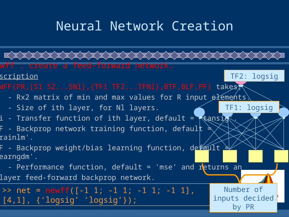
net = newff(PR,[S1 S2...SNl],{TF1 TF2...TFNl},BTF,BLF,PF) Description NEWFF(PR,[S1 S2...SNl],{TF1 TF2...TFNl},BTF,BLF,PF) takes, PR - Rx2 matrix of min and max values for R input elements. Si - Size of ith layer, for Nl layers. TFi - Transfer function of ith layer, default = 'tansig'. BTF - Backprop network training function, default = 'trainlm'. BLF - Backprop weight/bias learning function, default = 'learngdm'. PF - Performance function, default = 'mse’ and returns an N layer feed-forward backprop network.
Number of inputs decided by PR
S1: number hidden neurons
S2: number of ouput neuron
>> PR = [-1 1; -1 1; -1 1; -1 1];
-1 1 -1 1 -1 1 -1 1
Min Max
neuron 1
Neural Network Creation
newff : create a feed-forward network. Description NEWFF(PR,[S1 S2...SNl],{TF1 TF2...TFNl},BTF,BLF,PF) takes, PR - Rx2 matrix of min and max values for R input elements. Si - Size of ith layer, for Nl layers. TFi - Transfer function of ith layer, default = 'tansig'. BTF - Backprop network training function, default = 'trainlm'. BLF - Backprop weight/bias learning function, default = 'learngdm'. PF - Performance function, default = 'mse’ and returns an N layer feed-forward backprop network.
TF1: logsig
TF2: logsig
>> net = newff([-1 1; -1 1; -1 1; -1 1], [4,1], {‘logsig’ ‘logsig’}); Number of inputs decided by PR

Network Initialisation
Initialise the net’s weighting and biases>> net = init(net); % init is called after newff
re-initialise with other function:– net.layers{1}.initFcn = 'initwb';– net.inputWeights{1,1}.initFcn = 'rands';– net.biases{1,1}.initFcn = 'rands';– net.biases{2,1}.initFcn = 'rands';

Network Training
The overall architecture of your neural network is store in the variable net;
We can reset the variable inside.
net.trainParam.epochs =1000; (Max no. of epochs to train) [100]
net.trainParam.goal =0.01; (stop training if the error goal hit) [0]
net.trainParam.lr =0.001; (learning rate, not default trainlm) [0.01]
net.trainParam.show =1; (no. epochs between showing error) [25]
net.trainParam.time =1000; (Max time to train in sec) [inf]

Network Training(cont’d)
train : train the network with its architecture. Description TRAIN(NET,P,T,Pi,Ai) takes, NET - Network. P - Network inputs. T - Network targets, default = zeros. Pi - Initial input delay conditions, default = zeros. Ai - Initial layer delay conditions, default = zeros.
>> p = [-0.5 1 -0.5 1; -1 0.5 -1 0.5; 0.5 1 0.5 1; -0.5 -1 -0.5 -1];
-0.5 1 -0.5 1 -1 0.5 -1 0.5 0.5 1 0.5 1 -0.5 -1 -0.5 -1Training
pattern 1
For neuron 1

Network Training(cont’d)
train : train the network with its architecture. Description TRAIN(NET,P,T,Pi,Ai) takes, NET - Network. P - Network inputs. T - Network targets, default = zeros. Pi - Initial input delay conditions, default = zeros. Ai - Initial layer delay conditions, default = zeros.
>> p = [-0.5 1 -0.5 1; -1 0.5 -1 0.5; 0.5 1 0.5 1; -0.5 -1 -0.5 -1];
>> net = train(net, p, t);
>> t = [-1 1 -1 1];
-1 1 -1 1
Training pattern 1

Simulation of the network
[Y] = SIM(model, UT)
Y : Returned output in matrix or structure format. model : Name of a block diagram model. UT : For table inputs, the input to the model is interpolated.
>> UT = [-0.5 1 ; -0.25 1; -1 0.25 ; -1 0.5];
-0.5 1.00 -0.25 1.00 -1.00 0.25 -1.00 0.50Training
pattern 1
For neuron 1
>> Y = sim(net,UT);

Performance Evaluation
Comparison between target and network’s output in testing set.(generalisation ability)
Comparison between target and network’s output in training set. (memorisation ability)
Design a function to measure the distance/similarity of the target and output, or simply use mse for example.

Write them in a file(Adding a new function)
Create a file as fname.m (extension as .m)>> fname
loading.mfunction [Y , Z] = othername(str)
Y = load(str);
Z = length(Y);
>> [A,B] = loading('wtest.txt');

Reference
Neural Networks Toolbox User's Guide– http://www.cse.cuhk.edu.hk/corner/tech/doc/manual/matlab-5.3.1/help/pdf_doc/nnet/nnet.pdf
Matlab Help Desk– http://www.cse.cuhk.edu.hk/corner/tech/doc/manual/matlab-5.3.1/help/helpdesk.html
Mathworks ower of Matlab– http://www.mathworks.com/


