Neuro-Evolution Search Methodologies for Collective Self ...

Neuro-Evolution Search Methodologies for

Collective Self-Driving Vehicles

Chien-Lun (Allen) Huang

October 2019Version: 1.02 (Final)

Univers

ity of

Cap

e Tow

n

The copyright of this thesis vests in the author. No quotation from it or information derived from it is to be published without full acknowledgement of the source. The thesis is to be used for private study or non-commercial research purposes only.

Published by the University of Cape Town (UCT) in terms of the non-exclusive license granted to UCT by the author.

Univers

ity of

Cap

e Tow

n

University of Cape Town

Department of Computer Science

Computer Science

Neuro-Evolution Search Methodologies forCollective Self-Driving Vehicles


1. Reviewer Dr Geoff NitschkeDepartment of Computer ScienceUniversity of Cape Town

Supervisors Dr Geoff Nitschke

October 2019

Chien-Lun (Allen) HuangNeuro-Evolution Search Methodologies for Collective Self-Driving VehiclesComputer Science, October 2019University of Cape TownDepartment of Computer Science18 University AvenueRondeboschCape Town7700

Abstract

Recently there has been an increasing amount of research into autonomous vehiclesfor real-world driving. Much progress has been made in the past decade with manyautomotive manufacturers demonstrating real-world prototypes.

Current predictions indicate that roads designed exclusively for autonomous vehicleswill be constructed and thus this thesis explores the use of methods to automaticallyproduce controllers for autonomous vehicles that must navigate with each other onthese roads.

Neuro-Evolution, a method that combines evolutionary algorithms with neuralnetworks, has shown to be effective in reinforcement-learning, multi-agent taskssuch as maze navigation, biped locomotion, autonomous racing vehicles and fin-lessrocket control.

Hence, a neuro-evolution method is selected and investigated for the controllerevolution of collective autonomous vehicles in homogeneous teams.

The impact of objective and non-objective search (and a combination of both, ahybrid method) for controller evolution is comparatively evaluated for robustnesson a range of driving tasks and collection sizes.

Results indicate that the objective search was able to generalise the best on unseentask environments compared to all other methods and the hybrid approach was ableto yield desired task performance on evolution far earlier than both approaches butwas unable to generalise as effectively over new environments.

v

Acknowledgement

This thesis has been a long journey for me as I transitioned through various stagesof my life. It has taken far longer than I had originally planned and I am grateful toeveryone who believed in me and supported me along the way.

First, thank you to all who have funded my Masters. This includes the NationalResearch Foundation (NRF) and the Department of Science and Innovation (DSI)in collaboration with the Council for Scientific and Industrial Research (CSIR) forawarding me bursaries. My current employer, Allan Gray Proprietary Limited alsoprovided additional funding.

I would also like to thank my supervisor, Geoff for providing insight, inspriation andfor being patient as I slowly progressed with this thesis.

Finally, I am grateful to my family for always supporting me in all my endeavoursand my girlfriend, Suri for always being there and providing constant motivationand encouragement. I would also like to thank all my friends who helped proof-readthis thesis to ensure that it is of the highest quality.

Without you all, this research would not have been achievable.

Thank you.

vii

Contents

1 Introduction 1

1.1 Motivation and Problem Statement . . . . . . . . . . . . . . . . . . . 2

1.2 Methods . . . . . . . . . . . . . . . . . . . . . . . . . . . . . . . . . . 2

1.3 Contributions . . . . . . . . . . . . . . . . . . . . . . . . . . . . . . . 3

1.4 Thesis Structure . . . . . . . . . . . . . . . . . . . . . . . . . . . . . . 4

2 Background 7

2.1 Neuro-Evolution . . . . . . . . . . . . . . . . . . . . . . . . . . . . . 7

2.1.1 Artificial Neural Networks . . . . . . . . . . . . . . . . . . . . 7

2.1.2 Evolutionary Algorithms . . . . . . . . . . . . . . . . . . . . . 10

2.1.3 Evolving Neural Networks . . . . . . . . . . . . . . . . . . . . 12

2.1.4 Neuro-Evolution of Augmenting Topologies (NEAT) . . . . . . 15

2.1.5 Why NEAT? . . . . . . . . . . . . . . . . . . . . . . . . . . . . 20

2.2 Evolutionary Search Methods . . . . . . . . . . . . . . . . . . . . . . 21

2.2.1 Objective and Non-Objective search . . . . . . . . . . . . . . . 21

2.2.2 Novelty Search . . . . . . . . . . . . . . . . . . . . . . . . . . 22

2.2.3 Hybrid Search . . . . . . . . . . . . . . . . . . . . . . . . . . . 24

2.2.4 Applications . . . . . . . . . . . . . . . . . . . . . . . . . . . . 24

2.3 Autonomous Vehicles . . . . . . . . . . . . . . . . . . . . . . . . . . . 25

2.3.1 Controller Design . . . . . . . . . . . . . . . . . . . . . . . . . 25

2.3.2 Current Self-Driving Vehicles . . . . . . . . . . . . . . . . . . 28

2.4 Conclusion . . . . . . . . . . . . . . . . . . . . . . . . . . . . . . . . 29

3 Methods 31

3.1 Simulator and NEAT Implementation . . . . . . . . . . . . . . . . . . 31

3.2 Evaluation Functions . . . . . . . . . . . . . . . . . . . . . . . . . . . 32

3.2.1 Fitness Function . . . . . . . . . . . . . . . . . . . . . . . . . 32

3.2.2 Novelty Metric . . . . . . . . . . . . . . . . . . . . . . . . . . 32

3.2.3 Hybrid Function . . . . . . . . . . . . . . . . . . . . . . . . . 34

3.3 Conclusion . . . . . . . . . . . . . . . . . . . . . . . . . . . . . . . . 35

4 Experiments and Results 37

4.1 Vehicle Simulation . . . . . . . . . . . . . . . . . . . . . . . . . . . . 37

4.2 Task Environments . . . . . . . . . . . . . . . . . . . . . . . . . . . . 40

ix

4.2.1 Checkpoints . . . . . . . . . . . . . . . . . . . . . . . . . . . . 404.3 Neuro-Evolution Experiments . . . . . . . . . . . . . . . . . . . . . . 444.4 Generalisability Evaluations . . . . . . . . . . . . . . . . . . . . . . . 444.5 Results . . . . . . . . . . . . . . . . . . . . . . . . . . . . . . . . . . . 45

4.5.1 Neuro-Evolution (NE) Results . . . . . . . . . . . . . . . . . . 454.5.2 Generalisability Results . . . . . . . . . . . . . . . . . . . . . 474.5.3 Overall Evaluation Results . . . . . . . . . . . . . . . . . . . . 474.5.4 Evaluation Results by Vehicle Configuration . . . . . . . . . . 504.5.5 Evaluation Results by Track . . . . . . . . . . . . . . . . . . . 50

5 Discussion 575.1 Evolved Task Performance . . . . . . . . . . . . . . . . . . . . . . . . 575.2 Behavioural Space Analysis . . . . . . . . . . . . . . . . . . . . . . . 585.3 Generalisability Evaluations . . . . . . . . . . . . . . . . . . . . . . . 58

5.3.1 Controller Complexity . . . . . . . . . . . . . . . . . . . . . . 59

6 Conclusion 636.1 Summary of Findings and Results . . . . . . . . . . . . . . . . . . . . 636.2 Known Limitations . . . . . . . . . . . . . . . . . . . . . . . . . . . . 636.3 Future Work . . . . . . . . . . . . . . . . . . . . . . . . . . . . . . . . 64

Bibliography 65

x

1Introduction

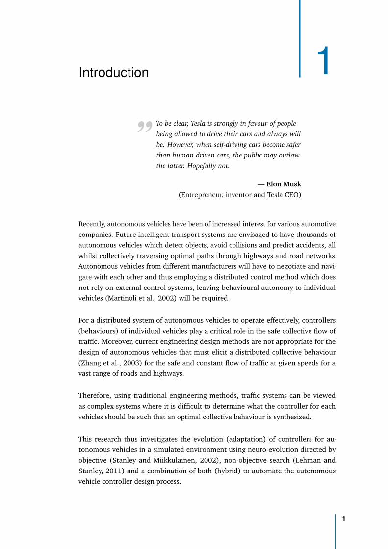
„To be clear, Tesla is strongly in favour of peoplebeing allowed to drive their cars and always willbe. However, when self-driving cars become saferthan human-driven cars, the public may outlawthe latter. Hopefully not.

— Elon Musk(Entrepreneur, inventor and Tesla CEO)

Recently, autonomous vehicles have been of increased interest for various automotivecompanies. Future intelligent transport systems are envisaged to have thousands ofautonomous vehicles which detect objects, avoid collisions and predict accidents, allwhilst collectively traversing optimal paths through highways and road networks.Autonomous vehicles from different manufacturers will have to negotiate and navi-gate with each other and thus employing a distributed control method which doesnot rely on external control systems, leaving behavioural autonomy to individualvehicles (Martinoli et al., 2002) will be required.

For a distributed system of autonomous vehicles to operate effectively, controllers(behaviours) of individual vehicles play a critical role in the safe collective flow oftraffic. Moreover, current engineering design methods are not appropriate for thedesign of autonomous vehicles that must elicit a distributed collective behaviour(Zhang et al., 2003) for the safe and constant flow of traffic at given speeds for avast range of roads and highways.

Therefore, using traditional engineering methods, traffic systems can be viewedas complex systems where it is difficult to determine what the controller for eachvehicles should be such that an optimal collective behaviour is synthesized.

This research thus investigates the evolution (adaptation) of controllers for au-tonomous vehicles in a simulated environment using neuro-evolution directed byobjective (Stanley and Miikkulainen, 2002), non-objective search (Lehman andStanley, 2011) and a combination of both (hybrid) to automate the autonomousvehicle controller design process.

1

1.1 Motivation and Problem Statement

Distributed autonomous vehicle control is a complex process, especially when col-lective behaviour needs to be synthesized. Moreover, current driving systems relyon vision, rather than more advanced technologies such as smart infrastructure orvehicle-to-vehicle communication. Current self-driving cars attempt to replicate hu-man actions but at a more efficient level, thus still relying on traditional vision-baseddriving requirements and road rules.

In the future, it is predicted that all vehicles on roads will be autonomous. If thissituation arises, the need for road rules that govern the way humans drive willno longer be appropriate and thus vehicles could rather travel in a more optimalfashion: simultaneously avoiding obstacles (other autonomous vehicles, road obsta-cles, pedestrians) and keeping within road barriers without the need for lanes orintersections that require stopping.

For this research we assume all vehicles will have fully-functioning sensor systems toproperly detect other vehicles and obstacles around it (for example, LIDAR sensors(Levinson et al., 2011)) along with a vehicle tracking system (for example, GPS(Space-Based Positioning and Timing, 2017)) so that vehicles are aware of theirpositions relative to its destination.

Autonomous vehicles will be tasked with navigating a simulated environment withvarious static and dynamic obstacles. These autonomous vehicles will need tocollectively navigate whilst avoiding collisions with each other and other obstacleswhilst minimising travel time by following the optimal path at high speeds and thusutilising energy effectively.

Currently, there is no distributed control system for collective fully-autonomousvehicles that must navigate roads whilst accounting for other autonomous vehicles,obstacles and unpredictable events such as pedestrians or animals crossing. Thisresearch attempts to address this gap by presenting neuro-evolution methods forthis application.

1.2 Methods

The main objective of this research is to automate the production of autonomousvehicle controllers that operate in a distributed fashion on any given environment.This means that controllers will be generalisable to unseen road networks that differ

2 Chapter 1 Introduction

from the training environment and be robust to different group sizes of autonomousvehicles.

Neuro-Evolution of Augmenting Topologies (NEAT) (Stanley and Miikkulainen,2002) is used to adapt the vehicle controllers. NEAT is an approach to adapt artificialneural networks by evolving network connection weights and the network’s structure(topology).

We investigate three methods: a traditional objective based approach (using afitness function): NEAT Objective Controller Evolution (OCE), a non-objective basedapproach: NEAT Novelty Controller Evolution (NCE) (based on novelty search (NS)by (Lehman and Stanley, 2011)), and a hybrid (HCE) approach where the fitnessfunction from OCE is combined with the novelty score from NCE.

In our experiments, vehicles act in homogeneous teams whereby morphology (shape,type, sensor configuration) and controller are the same for individual vehicles duringevolution process. Homogeneous (clones) teams allow for many instances of acontroller to be tested simultaneously, and is thus more efficient to adapt. Much ofthe literature uses homogeneous teams (Waibel et al., 2009) as they are easier to use(Trianni et al., 2006), scale more easily and are more robust to failures of individuals(Bryant and Miikkulainen, 2003) within teams when compared with heterogeneousteams (Floreano and Mattiussi, 2008). To adapt heterogeneous teams, each variantcontroller would compound the overall evaluation if it were to have been evolvedwith the same rigour as in the homogeneous team.

1.3 Contributions

NE has demonstrated the ability to produce ANN controllers that yield behaviourssuccessful at a wide variety of complex control tasks such as maze navigation, bipedlocomotion (Lehman and Stanley, 2011) and pole balancing (Gomez et al., 2006),along with a variety of autonomous driving research (Togelius and Lucas, 2006;Ebner and Tiede, 2009; Drchal and Koutník, 2009).

A non-objective search approach for NE, NS has also been demonstrated to out-perform (in terms of search speed and ability to avoid getting trapped in localoptima) traditional objective based methods in certain domains (Lehman and Stan-ley, 2011).

Furthermore, the combination of the objective and non-objective methods (a hybrid),has demonstrated the ability to outperform pure approaches (Huang et al., 2015).

1.3 Contributions 3

In this research, we assess the efficacy of traditional objective, novelty search and ahybrid methods on the collective autonomous driving task.

Prior research on autonomous driving using NE have focused on adapting controllersto navigate a single vehicle through a track using either objective or non-objectivemethods, rarely combining the two or adapting controllers to yield collective drivingbehaviours.

Given past research demonstrating the capability of hybrid approaches outperformingtraditional (pure) methods, we hypothesize that the hybrid approach will adaptcontrollers that will generalise more effectively across various unseen environmentswhen compared with the pure-objective and pure-novelty methods in this collectiveself-driving task.

The ability to successfully synthesize collective vehicle control behaviours could aidin designing future transportation systems where autonomous vehicle manufacturersdevelop safe and efficient autonomous fleets that do not rely on costly centralisedcontrol systems.

1.4 Thesis Structure

Chapter 2

This chapter provides the background of this research and introduces neuro-evolution,evolutionary search methods and autonomous vehicles.

Chapter 3

This chapter gives an overview of the specific implementations were employed forthis research including details of the simulator, implementation and parameters forNeuro-Evolution of Augmenting Topologies (NEAT), the evaluation functions definedfor each evolutionary search method and further details on our implementations fornovelty search (NS) and hybrid approaches.

Chapter 4

This chapter describes the experiments, simulated vehicles and environments alongwith all permutations of experiments undertaken to assess performance betweeneach search method. Results are then presented with graphs and statistical tests.

Chapter 5

The penultimate chapter presents a detailed analysis of the results and relates themback to the initial hypothesis.

4 Chapter 1 Introduction

Chapter 6

Finally, this chapter discusses the results and describes some limitations with thiswork and future research.

1.4 Thesis Structure 5

2Background

This chapter provides background on methods used in our research and a literaturereview of existing research on autonomous vehicle controller design. It is dividedinto three sections.

The first section introduces Neuro-Evolution (NE) and explores the underlyingtechnologies: artificial-neural networks (ANN) and evolutionary algorithms (EA).Neuro-Evolution of Augmenting Topologies (NEAT) is discussed in detail as it is themethod used to adapt vehicle controllers in this research. In section 2, evolutionarysearch methods are discussed with focus on objective, non-objective and hybridmethods to guide NE. The non-objective method, Novelty Search (NS) is elaboratedin more detail as it is the focus of this research.

In the final section, research in controller design for autonomous vehicles is surveyedand the current state-of-the-art self-driving technology in production and prototypevehicles outlined.

2.1 Neuro-Evolution

Neuro-Evolution (NE) is the evolution of Artificial Neural Networks using Evolution-ary Algorithms. NE thus combines the power of two biologically inspired methods:the brain and the evolutionary process that derived the brain over generations. NEpresents an alternative method to traditional reinforcement learning (RL) problemsas solutions are not modified during evaluations (ontogenetic) but rather, throughrecombination of individuals in a population. This population-based or phylogeneticlearning gradually moves the population towards the solution where an individualthat exhibits a desired behaviour on a given task (highest fitness) is found.

2.1.1 Artificial Neural Networks

Artificial Neural Networks (ANN) is a computational model based on the biologicalneural networks found in the natural brain. ANNs are powerful problem solvers asthey are universal function approximators, are generalisable and can retain memory(through recurrent networks) (Gomez, 2003). Similar to how a brain’s neural

7

network is comprised of a vast array of neurons and their connections (axons anddendrites), an ANN is created by combining multiple artificial neurons.

The artificial neuron (depicted in the inset in figure 2.1) is a referred to as a nodeand it receives inputs via its input connections and produces a single output basedon the input connection’s weights and the node’s activation function. The inputvalues from the input connections are multiplied by the connection weights and abias value is added to create a net input value using the following equation:

z =∑i

wijOi + θj (2.1)

where wij is the weight between current node j and incoming node i, Oi is theoutput value of node i and θj is the bias.

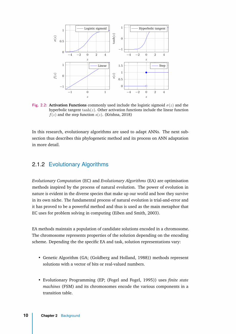
The net input, z is then passed to the activation function. Figure 2.2 depicts fourcommonly used activation functions. The output from this node thus depends on itsinputs and the type of activation function used (for example, if a sigmoid functionwas selected, the output would be: σ(z)).

Multiple neurons are connected together to form an ANN. In the application ofsuch networks, the structure, connection weights or both are modified and tunedto enable it to learn and create desirable outputs based on given inputs. Figure 2.1depicts a fully-connected feed-forward neural network with a total of 10 nodes (4input nodes, 5 hidden substrate nodes and one output node). Layers are used todescribe where nodes reside in the network. Input nodes are in the input layer andthese nodes have no incoming connections from other nodes. Output nodes are inthe output layer (they terminate and have no outgoing connections into other nodes)and nodes that have both incoming and outgoing connections to and from othernodes are referred to hidden nodes in the hidden layer. There can be any numberof hidden layers but only one input and one output layer. The network structure(number of nodes and connections between them) are referred to as the networktopology.

Each input node can receive some numerical feature or signal of the task or envi-ronment. In a supervised learning task, an example in image processing wouldmap each input node to a cluster of pixels on an image. Similarly, in reinforcementlearning such as control systems, inputs would be signals from sensors that receiveinformation about its environment. Outputs from these networks would either beclassification of an image or some action that is taken by the control system toinfluence the environment.

8 Chapter 2 Background

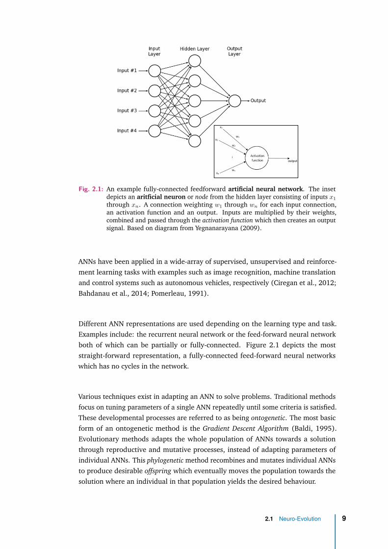
Fig. 2.1: An example fully-connected feedforward artificial neural network. The insetdepicts an aritficial neuron or node from the hidden layer consisting of inputs x1through xn. A connection weighting w1 through wn for each input connection,an activation function and an output. Inputs are multiplied by their weights,combined and passed through the activation function which then creates an outputsignal. Based on diagram from Yegnanarayana (2009).

ANNs have been applied in a wide-array of supervised, unsupervised and reinforce-ment learning tasks with examples such as image recognition, machine translationand control systems such as autonomous vehicles, respectively (Ciregan et al., 2012;Bahdanau et al., 2014; Pomerleau, 1991).

Different ANN representations are used depending on the learning type and task.Examples include: the recurrent neural network or the feed-forward neural networkboth of which can be partially or fully-connected. Figure 2.1 depicts the moststraight-forward representation, a fully-connected feed-forward neural networkswhich has no cycles in the network.

Various techniques exist in adapting an ANN to solve problems. Traditional methodsfocus on tuning parameters of a single ANN repeatedly until some criteria is satisfied.These developmental processes are referred to as being ontogenetic. The most basicform of an ontogenetic method is the Gradient Descent Algorithm (Baldi, 1995).Evolutionary methods adapts the whole population of ANNs towards a solutionthrough reproductive and mutative processes, instead of adapting parameters ofindividual ANNs. This phylogenetic method recombines and mutates individual ANNsto produce desirable offspring which eventually moves the population towards thesolution where an individual in that population yields the desired behaviour.

2.1 Neuro-Evolution 9

−4 −2 0 2 40

0.5

1

z

σ(z

)

Logistic sigmoid

−4 −2 0 2 4−1

0

1

z

tanh

(z)

Hyperbolic tangent

−1 0 1−1

0

1

z

f(z

)

Linear

−4 −2 0 2 4

0

0.5

1

1.5

z

s(z)

Step

Fig. 2.2: Activation Functions commonly used include the logistic sigmoid σ(z) and thehyperbolic tangent tanh(z). Other activation functions include the linear functionf(z) and the step function s(z). (Krishna, 2018)

In this research, evolutionary algorithms are used to adapt ANNs. The next sub-section thus describes this phylogenetic method and its process on ANN adaptationin more detail.

2.1.2 Evolutionary Algorithms

Evolutionary Computation (EC) and Evolutionary Algorithms (EA) are optimisationmethods inspired by the process of natural evolution. The power of evolution innature is evident in the diverse species that make up our world and how they survivein its own niche. The fundamental process of natural evolution is trial-and-error andit has proved to be a powerful method and thus is used as the main metaphor thatEC uses for problem solving in computing (Eiben and Smith, 2003).

EA methods maintain a population of candidate solutions encoded in a chromosome.The chromosome represents properties of the solution depending on the encodingscheme. Depending the the specific EA and task, solution representations vary:

• Genetic Algorithm (GA; (Goldberg and Holland, 1988)) methods representsolutions with a vector of bits or real-valued numbers.

• Evolutionary Programming (EP; (Fogel and Fogel, 1995)) uses finite statemachines (FSM) and its chromosomes encode the various components in atransition table.


• Genetic Programming (GP; (Koza, 1994)) uses tree-structures and thus chro-mosomes encode each node and branch.

• Neuro-Evolution (NE; (Wieland, 1991)) evolves ANNs and thus chromosomesencode the network structure and connection weights in some way and isdiscussed in further detail in section 2.1.3.

For example, using a GA to solve the Travelling Salesman Problem (Applegate et al.,2006) (a travelling salesman visiting multiple cities has to minimise travel distance.The task is to find the shortest path), an appropriate encoding of this problemwould be to store each city’s identifier as a gene in the solution’s genotype. Eachsubsequent gene would store the next city the salesman should travel to and thusthis representation maps directly to the problem whereby cities and order of travelis encoded (Grefenstette et al., 1985).

The EA process is a guided-random (stochastic) search which proceeds as follows:

1. A population of candidate solutions are initialised - either randomly or using aheuristic. Invalid solutions are removed or prevented from being created bysome rule.

2. Each individual is evaluated against a criteria. A measure of fitness is assignedto the individuals.

3. Individuals are selected by a selection criteria (for example, fitness propor-tionate, elitism) which are then recombined to produce offspring (Eiben andSmith, 2003). Invalid or damaged offspring are either discarded and recreatedor prevented from being produced.

4. Offspring are mutated and then evaluated where fitness is assigned to eachoffspring.

5. Using a replacement criteria (for example: fitness based, elitism), offspringreplace parents in the population.

6. Steps 2 - 5 are repeated until a stopping condition (solution found or maximumnumber of evaluations) is met.

Selection pressure in steps 3 (recombining solutions that perform well) and 5(replacing weak parents with fit offspring) forces newer generations to have highfitness and thus guides the search in finding good solutions in a reasonable time.


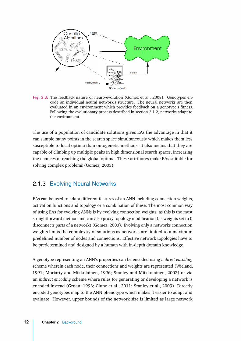
Fig. 2.3: The feedback nature of neuro-evolution (Gomez et al., 2008). Genotypes en-code an individual neural network’s structure. The neural networks are thenevaluated in an environment which provides feedback on a genotype’s fitness.Following the evolutionary process described in section 2.1.2, networks adapt tothe environment.

The use of a population of candidate solutions gives EAs the advantage in that itcan sample many points in the search space simultaneously which makes them lesssusceptible to local optima than ontogenetic methods. It also means that they arecapable of climbing up multiple peaks in high dimensional search spaces, increasingthe chances of reaching the global optima. These attributes make EAs suitable forsolving complex problems (Gomez, 2003).

2.1.3 Evolving Neural Networks

EAs can be used to adapt different features of an ANN including connection weights,activation functions and topology or a combination of these. The most common wayof using EAs for evolving ANNs is by evolving connection weights, as this is the moststraightforward method and can also proxy topology modification (as weights set to 0disconnects parts of a network) (Gomez, 2003). Evolving only a networks connectionweights limits the complexity of solutions as networks are limited to a maximumpredefined number of nodes and connections. Effective network topologies have tobe predetermined and designed by a human with in-depth domain knowledge.

A genotype representing an ANN’s properties can be encoded using a direct encodingscheme wherein each node, their connections and weights are represented (Wieland,1991; Moriarty and Mikkulainen, 1996; Stanley and Miikkulainen, 2002) or viaan indirect encoding scheme where rules for generating or developing a network isencoded instead (Gruau, 1993; Clune et al., 2011; Stanley et al., 2009). Directlyencoded genotypes map to the ANN phenotype which makes it easier to adapt andevaluate. However, upper bounds of the network size is limited as large network


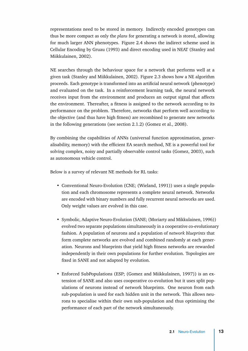
representations need to be stored in memory. Indirectly encoded genotypes canthus be more compact as only the plans for generating a network is stored, allowingfor much larger ANN phenotypes. Figure 2.4 shows the indirect scheme used inCellular Encoding by Gruau (1993) and direct encoding used in NEAT (Stanley andMiikkulainen, 2002).

NE searches through the behaviour space for a network that performs well at agiven task (Stanley and Miikkulainen, 2002). Figure 2.3 shows how a NE algorithmproceeds. Each genotype is transformed into an artificial neural network (phenotype)and evaluated on the task. In a reinforcement learning task, the neural networkreceives input from the environment and produces an output signal that affectsthe environment. Thereafter, a fitness is assigned to the network according to itsperformance on the problem. Therefore, networks that perform well according tothe objective (and thus have high fitness) are recombined to generate new networksin the following generations (see section 2.1.2) (Gomez et al., 2008).

By combining the capabilities of ANNs (universal function approximation, gener-alisability, memory) with the efficient EA search method, NE is a powerful tool forsolving complex, noisy and partially observable control tasks (Gomez, 2003), suchas autonomous vehicle control.

Below is a survey of relevant NE methods for RL tasks:

• Conventional Neuro-Evolution (CNE; (Wieland, 1991)) uses a single popula-tion and each chromosome represents a complete neural network. Networksare encoded with binary numbers and fully recurrent neural networks are used.Only weight values are evolved in this case.

• Symbolic, Adaptive Neuro-Evolution (SANE; (Moriarty and Mikkulainen, 1996))evolved two separate populations simultaneously in a cooperative co-evolutionaryfashion. A population of neurons and a population of network blueprints thatform complete networks are evolved and combined randomly at each gener-ation. Neurons and blueprints that yield high fitness networks are rewardedindependently in their own populations for further evolution. Topologies arefixed in SANE and not adapted by evolution.

• Enforced SubPopulations (ESP; (Gomez and Miikkulainen, 1997)) is an ex-tension of SANE and also uses cooperative co-evolution but it uses split pop-ulations of neurons instead of network blueprints. One neuron from eachsub-population is used for each hidden unit in the network. This allows neu-rons to specialise within their own sub-population and thus optimising theperformance of each part of the network simultaneously.


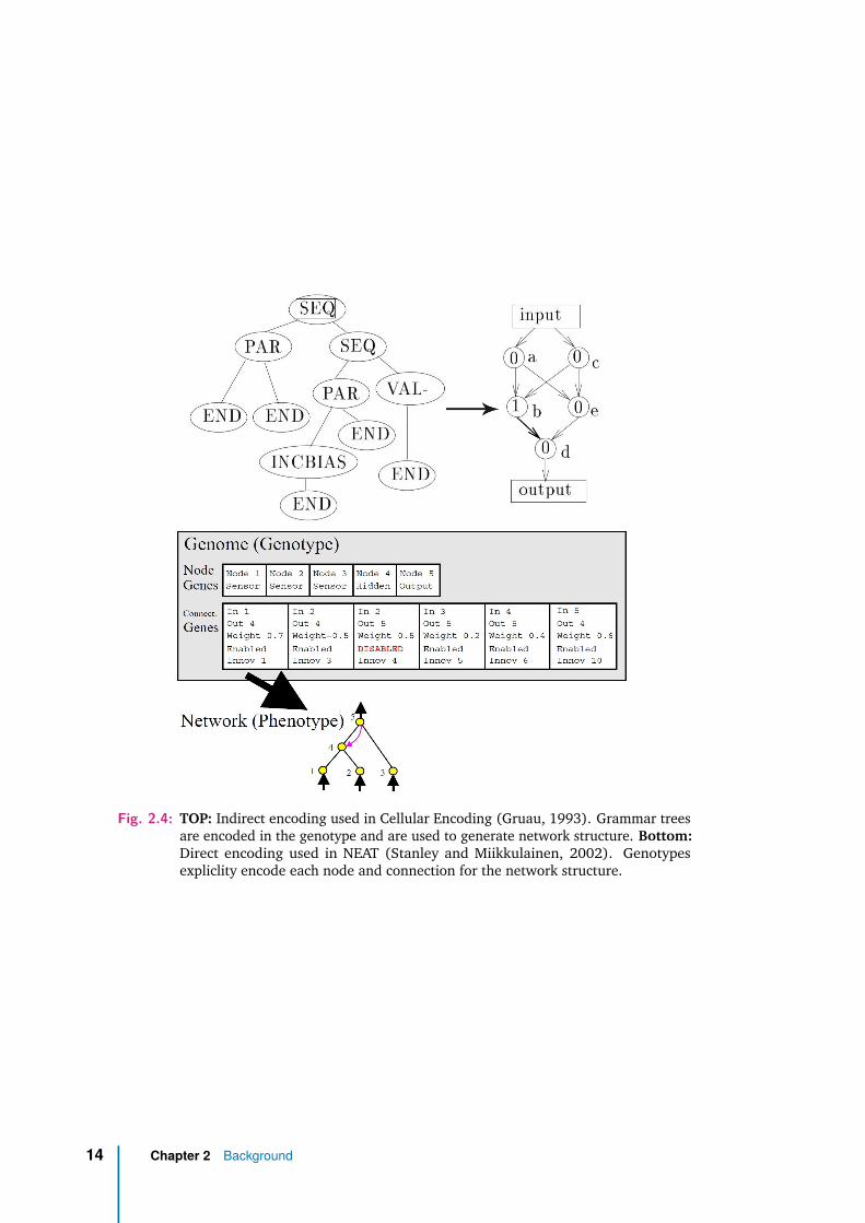
Fig. 2.4: TOP: Indirect encoding used in Cellular Encoding (Gruau, 1993). Grammar treesare encoded in the genotype and are used to generate network structure. Bottom:Direct encoding used in NEAT (Stanley and Miikkulainen, 2002). Genotypesexpliclity encode each node and connection for the network structure.


• GeNeralized Acquisition of Recurrent Links (GNARL; (Angeline et al., 1994))is a Topology and Weight Evolving Artificial Neural Networks (TWEANN) thatspecifically adapts recurrent networks. GNARL only performs mutation ongenotypes as authors question the efficacy of recombination.

• Neuro-Evolution of Augmenting Topologies (NEAT; (Stanley and Miikkulainen,2002)) is also a TWEANN. It uses a direct-encoding scheme and starts offwith minimal networks, gradually increasing the network complexity by eitheradding more nodes or connections. NEAT employs both mutation and recombi-nation and solves many issues plaguing topology adaptation in past TWEANNalgorithms. NEAT is described in further detail in the next section, as it is thefocus of this research.

2.1.4 Neuro-Evolution of Augmenting Topologies (NEAT)

Neuro-Evolution of Augmenting Topologies (NEAT) is a Topology and Weight Evolv-ing Artificial Neural Networks (TWEANNs) by Stanley and Miikkulainen (2002). Itis a complexification algorithm in that it starts out with very simple, minimal neuralnetworks and progressively increases the number of neurons and connections be-tween them. This process is analogical to biological evolution where species increasein complexity over evolutionary generations.

The advantage of using a complexification algorithm, such as NEAT for evolvingANNs, is due to the progressive difficulty of training increasingly complex (manynodes, layers and connections between them) networks. Furthermore, a simplenetwork might achieve similar results to a complex network, but with the advantageof being easier to evolve without changing their behaviour drastically and thusavoiding large networks that are slower to adapt.

Representation

The NEAT algorithm uses a direct genetic encoding that is designed to allow corre-sponding genes to be easily lined up during recombination. A genotype1 consistsof multiple genes (see figure 2.4 Bottom). The authors chose direct over indirectencoding as it does not restrict the phenotype networks and they demonstrate ex-perimentally that an indirect encoded algorithm (Cellular Encoding (Gruau, 1993))is not necessarily more efficient than a direct encoded algorithm (Stanley and Mi-ikkulainen, 2002). Furthermore, upper-bound network size limitations for direct

1A genotype’s gene in NEAT specifies one connection between nodes whilst the whole genotyperepresents the complete ANN.


encoding scheme does not affect this method as NEAT is biased towards solutionsthat have minimal networks.

Each gene has historical markings known as innovation numbers which denote whenthe gene was added. This unique feature in NEAT solves two problems experiencedby TWEANN algorithms.

A common issue with TWEANNs is that structural changes (additions of connectionsor nodes) usually cause a drop in fitness as the addition is unlikely to bring utility assoon as it they are introduced and a few generations are required before they areoptimized. Such innovations to the structure are often discarded by the EA as theyare ranked lower in terms of fitness.

To address this and ensure topological diversity, many TWEANNs initialise thepopulation with a random collection of topologies. Solutions in these randompopulations may produce infeasible networks where nodes have no connectionsfrom its input and outputs and require additional effort to clean up. These randompopulations also take longer to optimize as they have larger number of parameters(often many unnecessary nodes and connections to achieve behaviours that can beelicited with smaller networks).

Instead of initialising a random population of large solutions, NEAT starts withminimal networks and protect innovations by using its innovation numbers to nicheor speciate genotypes (group individuals with genetic similarity) to prevent themfrom being evaluated with the whole population. Fitness sharing in a species ofgenotypes is employed by NEAT and giving new genes some time to adapt, protectinginnovative genes from being discarded. The ability to protect innovations also allowsNEAT to minimise network sizes throughout evolution without having to incorporatea penalty on network size in the fitness function as in Zhang and Muhlenbein (1993),which may have undesirable effects of on the search and requires further tuning asit is unclear what the penalty should be in relation to task performance.

Since NEAT uses a direct encoding scheme, solutions that are genetically similarare topologically similar and thus niches are groups of networks that are similar instructure (see 2.1.4).

The second issue in TWEANNs is the Competing Conventions Problem where there aremany genotypic ways to express a solution. When genotypes that are functionallyequivalent crossover, they are likely to produce damaged offspring. Innovationnumbers allow genes that are equivalent in two different genotypes to line-up solvingthe problem.


Speciation

The innovation numbers allow us to line-up genes in a genotype that are similarand determine disjoint and excess genes. The number of disjoint and excess genesbetween solutions (see figure 2.7) can thus be used as a measure of compatibilitydistance between a pair of genotypes:

δ = c1E

N+ c2D

N+ c3 ·W (2.2)

where E and D is the number of excess and disjoint genes and W , the averageweight differences of matching genes (including disabled genes). c1, c2 and c3 areconstants that are adjusted to weight importance of each of the three factors and Nis the number of genes in the larger genotype, used for normalisation. The distancemeasure δ allows speciation of genotypes using a compatibility threshold δt.

The the end of a generation, each genotype (g) in the population is placed intospecies. Compatibility is determined for each species s sequentially (via a maintainedlist of species, S) by using a random representative genotype (sg). The genotype isplaced in first the specie where genotype’s δ(g, sg) ≤ δt. The average compatibilityof g compared with all the genotypes in s, but practically, using a single genotype(sg) is sufficient and faster (constant time). If g is not compatible with any species(∀s ∈ S, δ(g, sg) > δt), a new species is created and g becomes a member of the news.

Explicit fitness sharing is used within species, this means that all individuals inthe species share the niche’s fitness. This fitness of an individual, i is calculatedaccording to the distance δ from every other individual j.

Competing Conventions

The competing conventions problem also known as the permutations problem is whenthere is more than one way to express a neural network solution. When genotypesrepresenting the same solution do not have the same encoding, crossover is likelyto produce damaged offspring. Figure 2.5 depicts the problem for a solution withthree hidden nodes in two permutations. The hidden nodes can be configured in3! = 6 different permutations (in general, for n hidden nodes in a network, thereare n! functionally equivalent permutations) and when one of these permutationsrecombines with another, critical information in the network is lost. For example,


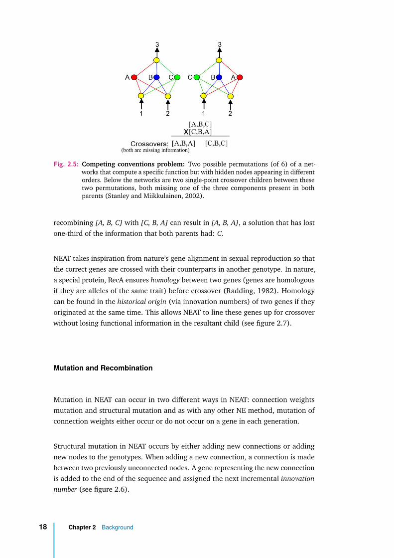
Fig. 2.5: Competing conventions problem: Two possible permutations (of 6) of a net-works that compute a specific function but with hidden nodes appearing in differentorders. Below the networks are two single-point crossover children between thesetwo permutations, both missing one of the three components present in bothparents (Stanley and Miikkulainen, 2002).

recombining [A, B, C] with [C, B, A] can result in [A, B, A], a solution that has lostone-third of the information that both parents had: C.

NEAT takes inspiration from nature’s gene alignment in sexual reproduction so thatthe correct genes are crossed with their counterparts in another genotype. In nature,a special protein, RecA ensures homology between two genes (genes are homologousif they are alleles of the same trait) before crossover (Radding, 1982). Homologycan be found in the historical origin (via innovation numbers) of two genes if theyoriginated at the same time. This allows NEAT to line these genes up for crossoverwithout losing functional information in the resultant child (see figure 2.7).

Mutation and Recombination

Mutation in NEAT can occur in two different ways in NEAT: connection weightsmutation and structural mutation and as with any other NE method, mutation ofconnection weights either occur or do not occur on a gene in each generation.

Structural mutation in NEAT occurs by either adding new connections or addingnew nodes to the genotypes. When adding a new connection, a connection is madebetween two previously unconnected nodes. A gene representing the new connectionis added to the end of the sequence and assigned the next incremental innovationnumber (see figure 2.6).


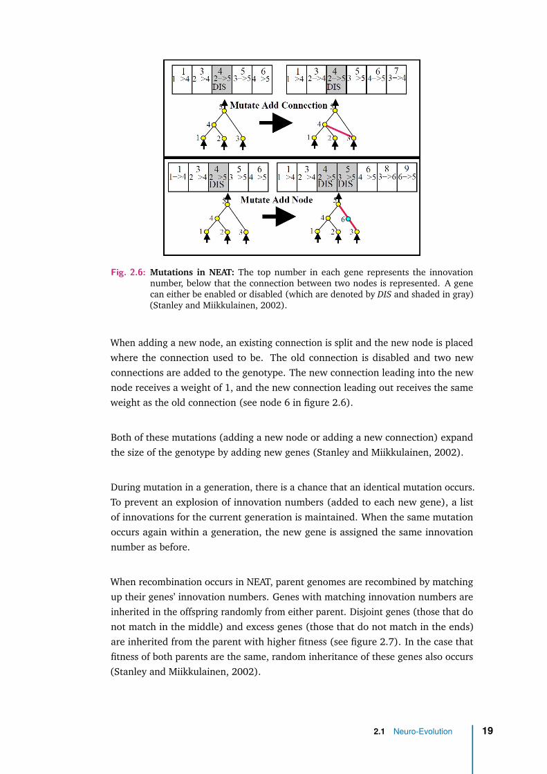
Fig. 2.6: Mutations in NEAT: The top number in each gene represents the innovationnumber, below that the connection between two nodes is represented. A genecan either be enabled or disabled (which are denoted by DIS and shaded in gray)(Stanley and Miikkulainen, 2002).

When adding a new node, an existing connection is split and the new node is placedwhere the connection used to be. The old connection is disabled and two newconnections are added to the genotype. The new connection leading into the newnode receives a weight of 1, and the new connection leading out receives the sameweight as the old connection (see node 6 in figure 2.6).

Both of these mutations (adding a new node or adding a new connection) expandthe size of the genotype by adding new genes (Stanley and Miikkulainen, 2002).

During mutation in a generation, there is a chance that an identical mutation occurs.To prevent an explosion of innovation numbers (added to each new gene), a listof innovations for the current generation is maintained. When the same mutationoccurs again within a generation, the new gene is assigned the same innovationnumber as before.

When recombination occurs in NEAT, parent genomes are recombined by matchingup their genes’ innovation numbers. Genes with matching innovation numbers areinherited in the offspring randomly from either parent. Disjoint genes (those that donot match in the middle) and excess genes (those that do not match in the ends)are inherited from the parent with higher fitness (see figure 2.7). In the case thatfitness of both parents are the same, random inheritance of these genes also occurs(Stanley and Miikkulainen, 2002).


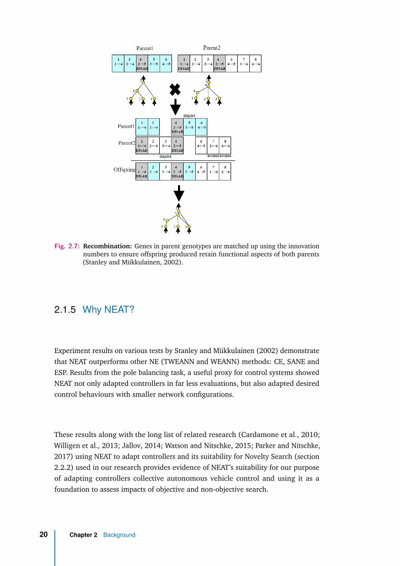
Fig. 2.7: Recombination: Genes in parent genotypes are matched up using the innovationnumbers to ensure offspring produced retain functional aspects of both parents(Stanley and Miikkulainen, 2002).

2.1.5 Why NEAT?

Experiment results on various tests by Stanley and Miikkulainen (2002) demonstratethat NEAT outperforms other NE (TWEANN and WEANN) methods: CE, SANE andESP. Results from the pole balancing task, a useful proxy for control systems showedNEAT not only adapted controllers in far less evaluations, but also adapted desiredcontrol behaviours with smaller network configurations.

These results along with the long list of related research (Cardamone et al., 2010;Willigen et al., 2013; Jallov, 2014; Watson and Nitschke, 2015; Parker and Nitschke,2017) using NEAT to adapt controllers and its suitability for Novelty Search (section2.2.2) used in our research provides evidence of NEAT’s suitability for our purposeof adapting controllers collective autonomous vehicle control and using it as afoundation to assess impacts of objective and non-objective search.


2.2 Evolutionary Search Methods

Different search methods are be used to guide the evolutionary process. In thissection, objective and non-objective search methods are described.

2.2.1 Objective and Non-Objective search

EAs require some criteria to evaluate individuals candidate solutions during thesearch process, as described in steps 2 - 4 in section 2.1.2 above.

This is often described as the objective or fitness function. The reason for thisnomenclature is due to a solution’s success measurement at a given task or objective.It measures how well a solution performs at a given task based on some functionpredetermined by the researcher. Furthermore, the choice of function to use canvary an EAs performance significantly.

Non-objective search methods, on the other hand, do not require researchers tocraft fitness functions to assess a genotype’s performance. Many researchers (Gould(1996), Miconi (2008) and Sigmund (1995)) have argued that fitness functions,which induce selection pressure (pressure to adapt in a certain way) actually restrictsthe search and opposes innovation.

In many problem domains, it is also extremely difficult to craft effective fitnessfunctions, as it requires an a priori understanding of the fitness landscapes andstepping stones to the objective (Woolley and Stanley, 2011). An oversight madeby the researcher when designing a fitness function could cause the search toprematurely converge or be trapped in local optima.

In a non objective method, stepping stones that would have been thrown away byan objective method because they appear to be far away from the objective, will bepreserved. These stepping stones may lead to the ultimate objectives and preventsolutions from getting trapped by deception (Lehman and Stanley, 2011)2.

Various non objective methods exist such as novelty search by Lehman and Stanley(2011) which explores the behaviour space instead of the problem space, curiosity-driven exploration by Pathak et al. (2017) which uses an intrinsic reward mechanism(prediction error as a proxy for curiosity) instead of extrinsic or objective rewards.

2Local optima that appear to be close to the objective, but prevents solutions from ever reaching theultimate goal.

2.2 Evolutionary Search Methods 21

Despite the advantage of not having to craft fitness functions, non-objective searchstill requires the researcher to craft and use some other metric to determine solutionquality in a non-objective manner. One example would be the novelty metric in anon-objective method novelty search which is used to define how to measure solutionnovelty or behavioural distance.

2.2.2 Novelty Search

Novelty search is a non objective neuro-evolution algorithm, proposed by Lehmanand Stanley (2011) where solutions are rewarded by a novelty metric based onhow significantly different or novel their behaviours (phenotypes) are in respect toprevious solutions.

Novelty search presents a new way of traversing the search space. It operates on thepremise that novel solutions provide the stepping stones (ones that objective-basedmethods would have discarded as they appear to be too far away from the objective)to the final objective. This way, novelty search ensures that solutions are not trappedor deceived into a local optima, which plagues objective-based methods.

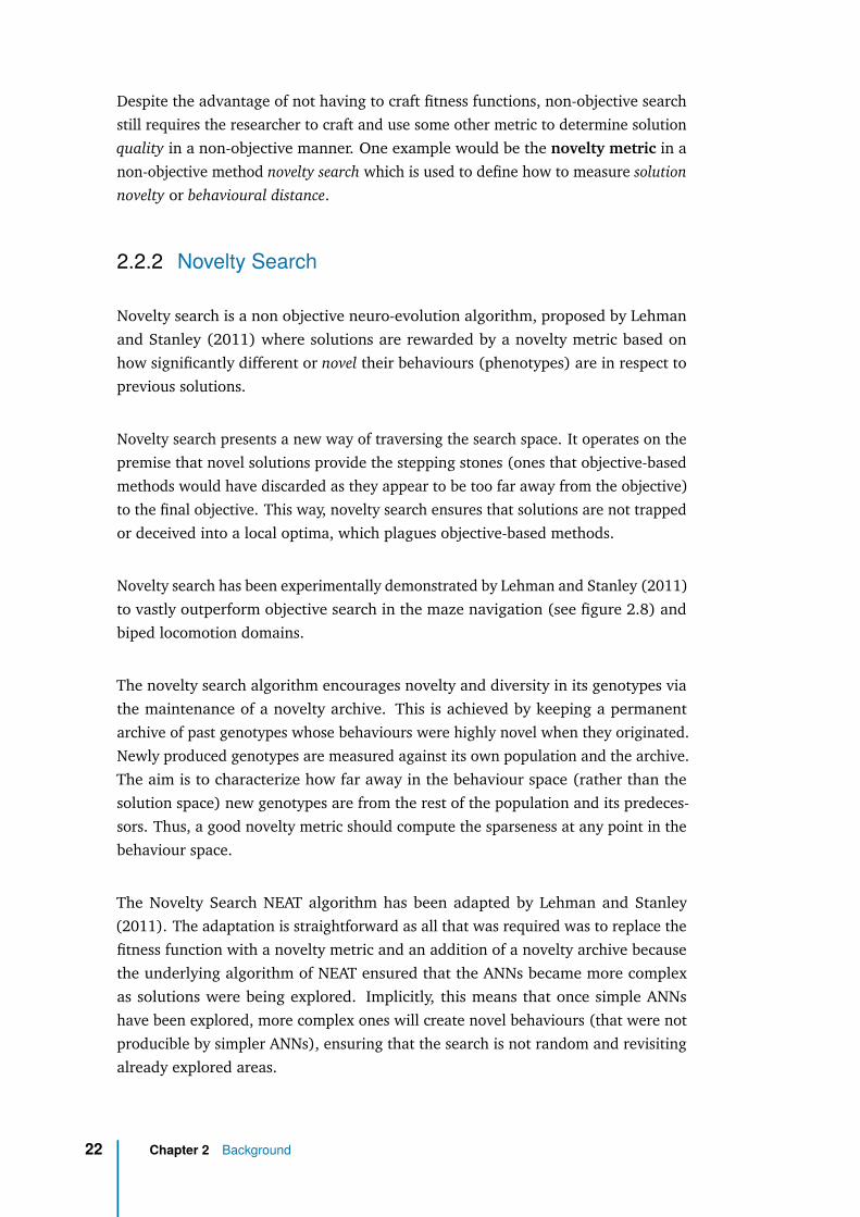
Novelty search has been experimentally demonstrated by Lehman and Stanley (2011)to vastly outperform objective search in the maze navigation (see figure 2.8) andbiped locomotion domains.

The novelty search algorithm encourages novelty and diversity in its genotypes viathe maintenance of a novelty archive. This is achieved by keeping a permanentarchive of past genotypes whose behaviours were highly novel when they originated.Newly produced genotypes are measured against its own population and the archive.The aim is to characterize how far away in the behaviour space (rather than thesolution space) new genotypes are from the rest of the population and its predeces-sors. Thus, a good novelty metric should compute the sparseness at any point in thebehaviour space.

The Novelty Search NEAT algorithm has been adapted by Lehman and Stanley(2011). The adaptation is straightforward as all that was required was to replace thefitness function with a novelty metric and an addition of a novelty archive becausethe underlying algorithm of NEAT ensured that the ANNs became more complexas solutions were being explored. Implicitly, this means that once simple ANNshave been explored, more complex ones will create novel behaviours (that were notproducible by simpler ANNs), ensuring that the search is not random and revisitingalready explored areas.


Fig. 2.8: Novelty Search Maze Navigation Resuts: starting positions in the medium (a, c)and hard (b, d) maps are located at the top left and bottom left, respectively. Theobjective or goal for the medium and hard maps are located at the bottom rightand top left, respectively. Each black dot represents the final locations of mazenavigation robots at the end of each evolution generation until either the goal orwhen the maximum number of evaluations were reached. In both maps, noveltywas able to traverse far more of the maze space earlier when compared to thefitness-based method. All methods were able to reach the goal with the exceptionof the hard map (d). The fitness function used was a distance of the navigatorsposition from the goal (straight-line distance). Novelty metric used to measurebehavioural sparsity: location (x, y co-ordinates) of the navigator (Lehman andStanley, 2011).

2.2 Evolutionary Search Methods 23

This implication shows that NEAT is an effective algorithm for novelty search andencourages exploration of the search space effectively.

2.2.3 Hybrid Search

Researchers (Cuccu and Gomez, 2011; Inden et al., 2013; Huang et al., 2015) havedemonstrated that combining objective and non-objective search methods can yieldsuperior performance over just using pure approaches.

Combination between objective and non-objective methods can be implementedin multiple ways. For purposes of illustration and due to our non-objective choice,Novelty Search, we will discuss combination methods between fitness and noveltysearch.

Selection by fitness and novelty: individuals in this hybrid method are selectedusing fitness-based tournament selection and novelty. A proportion of thepopulation are selected for based on their fitness and the remaining, novelty.(Inden et al., 2013)

Novelty-based speciation: instead of speciating individuals based on fitness orgenotypic similarity, species are maintained based on solutions’ behaviouralsimilarity. (Inden et al., 2013)

Weighted-sum of novelty and fitness: novelty scores and fitnesses are combinedlinearly to create a hybrid measure of performance. (Inden et al., 2013; Huanget al., 2015)

The weighted-sum approach was selected for its simplicity and its ability to out-perform nearly all other more complex methods in Inden et al., 2013 on the polebalancing, four patterns task.

2.2.4 Applications

Objective and non-objective search methods, specifically novelty search have beenused as evolutionary search methods across many applications. These include arange of simulated and physical task environments in the field of evolutionaryrobotics (ER).

Many (Gomez and Miikkulainen, 1999; Gomez et al., 2008; Igel, 2003) havedemonstrated the efficiency of using objective-based evolutionary search methods to


successfully solve the non-markovian double pole-balancing task. Later, it was shownthat non-objective and hybrid search methods are able to successfully solve the sametask with greater efficiency (Mouret and Doncieux, 2012; Cuccu and Gomez, 2011;Inden et al., 2013; Huang et al., 2015).

Although these tasks demonstrate the method’s feasibility in single-agent control,researchers have extended the literature with experiments using objective, non-objective and hybrid approaches for multi-agent and collective swarm ER tasks.

Gomes et al. (2013a), Gomes et al. (2016), and Nitschke and Didi (2017) haveshown that NE was suitable for multi-agent ER tasks and hybridizing objective andnon-objective search methods can yield better results.

Our research focuses on a multi-agent collective self-driving task where all vehicleshave homogeneous controllers testing various search methods.

2.3 Autonomous Vehicles

Recently there has been increasing research attention focused on overcoming thetechnical challenges for producing self-driving vehicles (KPMG, Center for Auto-motive Research, 2012). Some companies have demonstrated working productionprototypes (Ackerman, 2015), the successors of which are speculated as eventuallydisplacing the need for human drivers on public roads (Motavalli, 2012; Bilger, 2013;Bamonte, 2013).

Our research focus is on automated methods for deriving optimal controllers in self-driving vehicles that are able to generalise across new environments such as differentroad networks and traffic conditions. In this section we explore past research oncontroller and morphology design as well as the current state-of-the-art in terms ofself-driving vehicles in the real-world.

2.3.1 Controller Design

There has been a significant amount of work on evolving driving behaviours forsimulated (Togelius and Lucas, 2006; Ebner and Tiede, 2009; Drchal and Koutník,2009; Talamini et al., 2018) and physical vehicles (Beeson et al., 2008; Kestinget al., 2010; Furda and Vlacic, 2011) though such studies produce controllers thatare suitable for the given task environment and evolved driving behaviours rarelyfunction across a broad range of environments (Togelius and Lucas, 2005; Togeliusand Lucas, 2006; Cardamone et al., 2010).

2.3 Autonomous Vehicles 25

In Togelius and Lucas (2006), ANNs were utilised and a 3-layer neural network withfixed topology was used. The input layer consisted of at least three input nodes,a bias input of value 1, an input for the speed of the vehicle and an input for thewaypoint sensor. Each vehicle had a waypoint sensor which informed the networkat what angle the vehicle was approaching the next waypoint on the track. Furtherinputs were from range-finder or laser sensors with values of distances to obstaclesrecorded by each sensor. The network finally had two outputs, which were for thevehicle’s throttle and steering. Only the connection weights were adapted by the EA.The test environment was a 2-dimensional top-down simulation, with no physicssimulation other than moving the vehicle in the direction of travel and collisiondetection with walls.

Ebner and Tiede (2009) demonstrated a method of evolving controllers using GeneticProgramming. Genetic programming is another EA that is out of the scope of thisresearch, however, of interest in this particular research is that they used The openrace car simulator (TORCS), which is a more realistic 3-dimensional racing simulatorwith more realistic physics (gravity, friction) simulation. Similarly, Cardamone et al.(2010) also used the TORCS framework but utilized NE, specifically online-NE tolearn on-the-fly so that trained controllers can learn to drive on new tracks. In bothinstances however, the task was limited to driving a single vehicle around a racetrackas fast as possible, avoiding the track barriers.

Drchal and Koutník (2009) used ANNs for their vehicle controllers and HyperNEATas the EA. Here, both network weights and topologies were evolved with HyperNEAT,a variant of NEAT that uses indirect encoding. Simple two-wheeled vehicles weretrained to drive around an inter-connected roadway. Vehicles had to stay within theboundaries of the road, and not collide with each other if they had to cross paths.The output of the network controlled each wheel individually, thus allowing turnsand rotations to be made. Figure 2.9 provides an overview of past research.

Talamini et al. (2018) assessed the impact of ANN evolution using global (system-wide) versus local (individual vehicle) fitness in terms of speed, safety and efficiencyfor a collective driving task using NEAT in a simulated two-dimensional environment.Individual vehicles had five laser sensors spread out in 180◦ which provided inputinto the network for three distances: to the closest car, to the closest roadside,and to the closest intersection. Besides these three inputs from each sensor, threeadditional inputs were added: current car speed, distance to the target and directionof the target resulting in 18 input nodes. There were two outputs from the network:steering and acceleration (or braking, in the case of negative acceleration). Resultsdid not show statistical significance between local (selfish) and global optimisationbut did show that selfish fitness may yield more robust controllers, generalisableto different environments. Although this task was collective, vehicles started at


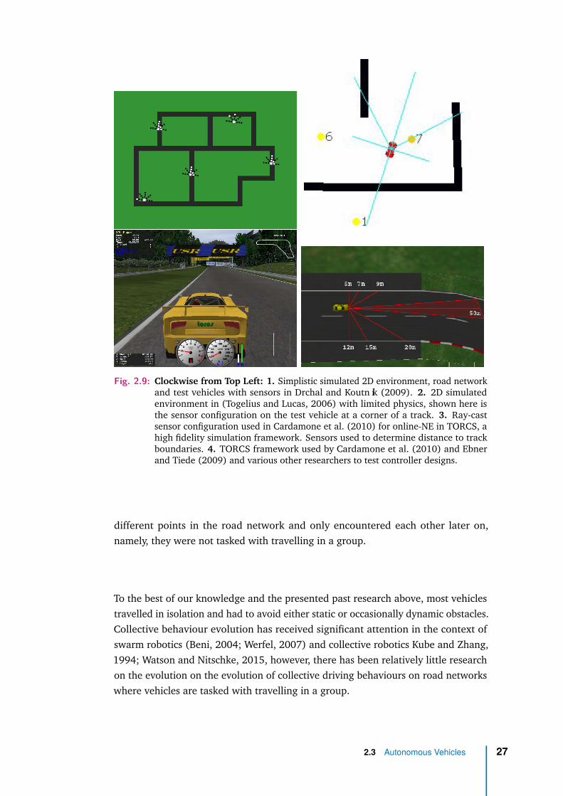
Fig. 2.9: Clockwise from Top Left: 1. Simplistic simulated 2D environment, road networkand test vehicles with sensors in Drchal and Koutník (2009). 2. 2D simulatedenvironment in (Togelius and Lucas, 2006) with limited physics, shown here isthe sensor configuration on the test vehicle at a corner of a track. 3. Ray-castsensor configuration used in Cardamone et al. (2010) for online-NE in TORCS, ahigh fidelity simulation framework. Sensors used to determine distance to trackboundaries. 4. TORCS framework used by Cardamone et al. (2010) and Ebnerand Tiede (2009) and various other researchers to test controller designs.

different points in the road network and only encountered each other later on,namely, they were not tasked with travelling in a group.

To the best of our knowledge and the presented past research above, most vehiclestravelled in isolation and had to avoid either static or occasionally dynamic obstacles.Collective behaviour evolution has received significant attention in the context ofswarm robotics (Beni, 2004; Werfel, 2007) and collective robotics Kube and Zhang,1994; Watson and Nitschke, 2015, however, there has been relatively little researchon the evolution on the evolution of collective driving behaviours on road networkswhere vehicles are tasked with travelling in a group.

2.3 Autonomous Vehicles 27

2.3.2 Current Self-Driving Vehicles

Due to the rapid interest by automotive companies to produce autonomous vehicles,significant progress has been made in the past few years. This section will providea survey of current production and prototype vehicles by various automotive andtechnology companies.

Furthermore, the National Highway Traffic Safety Administration (NHTSA) hasproposed a formal classification system (Highway and Administration, 2013) fordifferent levels of vehicle autonomy.

• No-Automation (Level 0): The driver is in complete and sole control of theprimary vehicle controls – brake, steering, throttle, and motive power – at alltimes.

• Function-specific Automation (Level 1): Automation at this level involvesone or more specific control functions. Examples include electronic stabilitycontrol or pre-charged brakes, where the vehicle automatically assists withbraking to enable the driver to regain control of the vehicle or stop fasterthan possible by acting alone. Almost all modern vehicles have this level ofautonomy as ESC and Anti-lock braking systems (ABS) are now mandatory forall new vehicles sold in the United States. (NHTSA, 2016)

• Combined Function Automation (Level 2): This level involves automation ofat least two primary control functions designed to work in unison to relieve thedriver of control of those functions. This level of autonomy is often achievedby utilizing radar technology combined with camera imaging techniques todetermine road bounds and "follow" traffic at safe distances. An example ofcombined functions enabling a Level 2 system is adaptive cruise control incombination with lane centering. Tesla’s autopilot in its Model S, Model 3 andModel X’s is currently considered Level 2 autonomy. (Kenwell, 2018)

• Limited Self-Driving Automation (Level 3): Vehicles at this level of automa-tion enable the driver to cede full control of all safety-critical functions undercertain traffic or environmental conditions and in those conditions to relyheavily on the vehicle to monitor for changes in those conditions requiringtransition back to driver control. The driver is expected to be available foroccasional control, but with sufficiently comfortable transition time. This levelrequires a larger suite of sensors, cameras and advanced image recognitionsoftware (often using deep-learning) to determine the bounds of the road androad obstacles. Highly-detailed maps are often required for accurate naviga-


tion and pre-planning to aid with the rest of the control systems. Waymo’sself-driving car is an example of limited self-driving automation. Recently, Audihas launched an A8 with Level 3 autonomy capabilities. (Wasef, 2018)

• Full Self-Driving Automation (Level 4): The vehicle is designed to performall safety-critical driving functions and monitor roadway conditions for anentire trip. Such a design anticipates that the driver will provide destination ornavigation input, but is not expected to be available for control at any timeduring the trip. This includes both occupied and unoccupied vehicles.

Almost all new vehicles today have Level 1 as a safety standard and Level 2 is oftenan optional safety feature available from many manufacturers. A few manufacturershave released either production (such as Tesla’s vehicles for a short period) orexperimental vehicles (Waymo’s self-driving vehicles) and Audi demonstrating Level3 capabilities.

2.4 Conclusion

In this chapter, evolutionary algorithms, neuro-evolution with a focus on NEAT andNovelty Search were reviewed. These are algorithms employed in this research forthe collective self-driving task. A survey of existing literature on self-driving researchusing evolutionary methods were listed as well as state-of-the-art technology used inproduction self-driving capabilities of today’s road vehicles.

Current research using evolutionary methods is largely limited to training individualvehicles to drive and testing them in isolation and technologies used in today’s pro-duction vehicles have achieved level 3 autonomy. Furthermore, existing evolutionarymethods only use objective-based search.

Our research is focused on Level 4 or full automation by NHTSA’s classifications forself-driving vehicles traversing road and highway networks in a collective fashion.We utilize the NEAT neuro-evolution algorithm and investigate the impact of usingobjective-based and non-objective-based search methods to elicit collective self-driving behaviours where all vehicles traverse multiple routes simultaneously whilstavoiding each other and other obstacles en-route to their destination.

2.4 Conclusion 29

3Methods

The focus of this research is on adapting autonomous vehicles to traverse variousroad environments in a collection and assessing the performance impact of thesearch method used to guide evolution. This chapter describes the implementationdetails for the simulator used in this research, algorithmic implementations of NEAT(objective, non-objective and hybrid) and the evaluation functions used for eachsearch method.

3.1 Simulator and NEAT Implementation

An extension of UnityNEAT (developed by Jallov (2014)) based on SharpNEAT byGreen (2003) (written in C#) was used to simulate physically realistic 3D vehicles,sensors, roads and obstacles. Unity1 is a multi-platform game engine that allows foreasy development of 2D or 3D games.

The vehicle controllers are evolved with the goal of being able to maximize theaverage distance traversed (measured by way of checkpoints passed) on tracks withobstacles, perpendicular traffic and oncoming traffic whilst minimizing collisionswith obstacles and other vehicles. Sensory input and motor output layers are fixedand NEAT adapts the number of hidden layer nodes and connectivity betweensensory inputs and motor outputs.

The simulation is performed for homogenous teams where groups of vehicles travel-ling together on the track have identical controllers.

NEAT Parameters

The parameters used in NEAT for the experiments are outlined in table 4.1 anddiscribed in more detail in the next chapter. The default activation function employedby NEAT, the steepened sigmoid function is used for our research:

1http://unity3d.com

31

σz = 11 + e−4.9·z (3.1)

The sigmoid function σ(z) is graphed in figure 2.2, top-left.

3.2 Evaluation Functions

A focus area of this research is to investigate the different methods used to directevolutionary search in NEAT. To determine the impact these methods have on searchefficiency, this section will discuss the three different evolutionary search methodsused: objective search (fitness), novelty search (NS) and hybrid search. Experimentalset-up and parameters are described in more detail in the next chapter.

3.2.1 Fitness Function

In the objective search method, controllers were awarded a fitness equalling theportion of the track’s length covered (via checkpoints) over 45 simulation (task trial)iterations:

fitness(x) = 1cars

cars∑i=0

(cppassedcptotal

∗ 0.9coll) (3.2)

where cars represents the number of cars in a group, cppassed denoting the numberof checkpoints vehicles successfully pass, cptotal is the total number of check-pointson that track, and coll is the number of collisions2 that a vehicles was involved in.Collisions cause an exponential decay to the fitness of an individual, thus allowing theevolution to be lenient individuals that collide rarely but penalise them exponentiallyas collision counts increase.

Thus vehicle controllers that minimized the number of collisions and maximized thenumber of check-points passed, were selected for by NEAT.

3.2.2 Novelty Metric

The non-objective approach, NS, requires a novelty metric to determine an controller’sbehavioural novelty. This novelty is described by sparseness (equation 3.3), which

2The value of 0.9 for the base was selected after experimenting with a few other values duringpreliminary experiments. Values lower than 0.9 (in increments of 0.1) resulted in slower evolutionand often caused evolution to stagnate.

32 Chapter 3 Methods

is a combination of a behaviour characterisation (which describes an controller’sbehaviour) and a distance metric. An individual’s novelty is thus a relative scoreon how different its behaviour is compared to others in the population and noveltyarchive.

A novelty archive is maintained to store novel controllers as they appear ensuringthat previously novel behaviours are not lost and reappear during evolution.

K-nearest neighbours (composed of other behaviourally similar solutions in thenovelty archive and solutions in the population at the same given generation) areused to compute a controller’s sparseness and thus novelty. Sparseness is definedas:

Sparseness(x) = 1k

k∑i=0

dist(x, µi) (3.3)

where µ is the ith-nearest neighbor of x with respect to the novelty metric, andwhere the distance component in equation 3.3 uses the Euclidean distance derivedby the Pythagorean theorem (Gower, 1982).

Novelty Archive

The top fifteen of the population (100) most novel solutions at each generation areadded to the novelty archive. The novelty archive is unbounded which means themaximum size of the novelty archive is 15×ngenerations at the final generation. Table4.1 presents the archive size and addition rate for novelty search and population sizefor the experiments.

Behaviour Characterisations

The behaviour characterisation (BC) describes the dimensions(s) chosen for thenovelty metric and has an impact on the search as it induces pressure to exhibitnovel behaviour based given attributes. To ascertain which BC yields the highestperformance (relating to the task), three BCs were tested and compared:

• Speed: Individual vehicle’s velocity measured in meters per second (m/s).

3.2 Evaluation Functions 33

• Speed and Cohesion: Individual vehicle’s velocity and the distance betweenthe vehicles. The distance between the vehicles is the line-of-sight distance inmeters.

• Location: Vehicle locations (x and z coordinates) in the simulated environ-ment.

For each of the metrics, values were sampled at fixed time-steps in the simulationand vectors of behaviours were compared with each other to determine an individualsolution’s sparseness.

Behaviour Sampling

The behaviour characterisation is a vector comprised of values that are sampled atfixed intervals of 1/100th of total simulation time-steps per generation. Each valuein the vector is a dimension that is used to compare against other individuals usingthe pythagoras equation.

One hundred samples are collected for each vehicle (sampling rate, table 4.1) ina group and since each vehicle has their own values during sampling, the vectorof behaviour characterisation values are combined for each vehicle in the groupmaking a final vector used for sparseness calculation.

To ensure that an individual vehicle’s behaviour is compared to the most similarvehicle’s behaviour in another solution’s behaviour vector, the final behaviour vectoris sorted by the aggregate values of the sub-vectors.

3.2.3 Hybrid Function

The hybrid search method used in this research linearly combines novelty and fitnessas in Huang et al. (2015) to create a weighted sum. The score that each individualreceives for the hybrid method is defined as:

score(i) = ρ.fit(i) + (1− ρ).nov(i) (3.4)

Where, ρ = 0.5, combining fitness and novelty equally which are normalized accord-ing to:

fit(i) = fit(i)− fitminfitmax − fitmin

, nov(i) = nov(i)− novminnovmax − novmin

(3.5)

34 Chapter 3 Methods

Where, novmin, fitmin are the lowest novelty and fitness values in the population,respectively and novmax, fitmax are the highest.

It was shown in Huang et al. (2015) increasing or decreasing the ρ value biasedthe results heavily to either objective performance or NS performance. As it is alsounclear for general tasks whether objective or NS will perform better and only witha priori experiments for either pure approached will an experimenter know if it isbetter to bias a weighted-sum hybrid approach to either objective or fitness. Toremove this bias and leave ρ as a parameter-tuning excercise, we selected ρ = 0.5.

3.3 Conclusion

In this chapter, the simulator used for these experiments along with the NEAT imple-mentation was outlined and the three different evaluation function implementationsfor fitness, novelty search and hybrid described.

The behaviour characterisation for novelty search and hybrid may have effect onsearch performance and thus we comparatively assess three different metrics, speed;speed and cohesion and location.

For simplicity and supported by previous research, we create a equally-weightedlinearly-combined fitness-novelty hybrid approach that will be used to assess whetherour hypothesis that hybrid approaches can generalise over various task environmentsis correct.

3.3 Conclusion 35

4Experiments and Results

The ANN controllers are adapted by NEAT for each evolutionary search method, ob-jective, non-objective and hybrid. Thereafter, generalisability tests (evaluations) areperformed for each of the adapted controllers to determine performance differencesfor each search method.

This chapter describes the simulated vehicles, task environments and experimentsthat will be run followed by results.

4.1 Vehicle Simulation

The vehicles in this simulation have a BMW E46 M3 body model. The simulationvehicle has similar acceleration and braking to that of a real-world vehicle. Maximumsteering angle is 25◦ and top speed is capped at 120km/h.

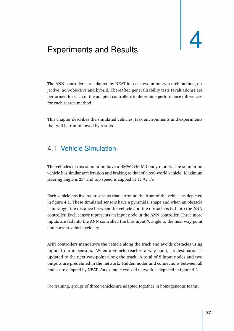
Each vehicle has five radar sensors that surround the front of the vehicle as depictedin figure 4.1. These simulated sensors have a pyramidal shape and when an obstacleis in range, the distance between the vehicle and the obstacle is fed into the ANNcontroller. Each sensor represents an input node in the ANN controller. Three moreinputs are fed into the ANN controller, the bias input θ, angle to the next way-pointand current vehicle velocity.

ANN controllers manoeuvre the vehicle along the track and avoids obstacles usinginputs from its sensors. When a vehicle reaches a way-point, its destination isupdated to the next way-point along the track. A total of 8 input nodes and twooutputs are predefined in the network. Hidden nodes and connections between allnodes are adapted by NEAT. An example evolved network is depicted in figure 4.2.

For training, groups of three vehicles are adapted together in homogeneous teams.

37

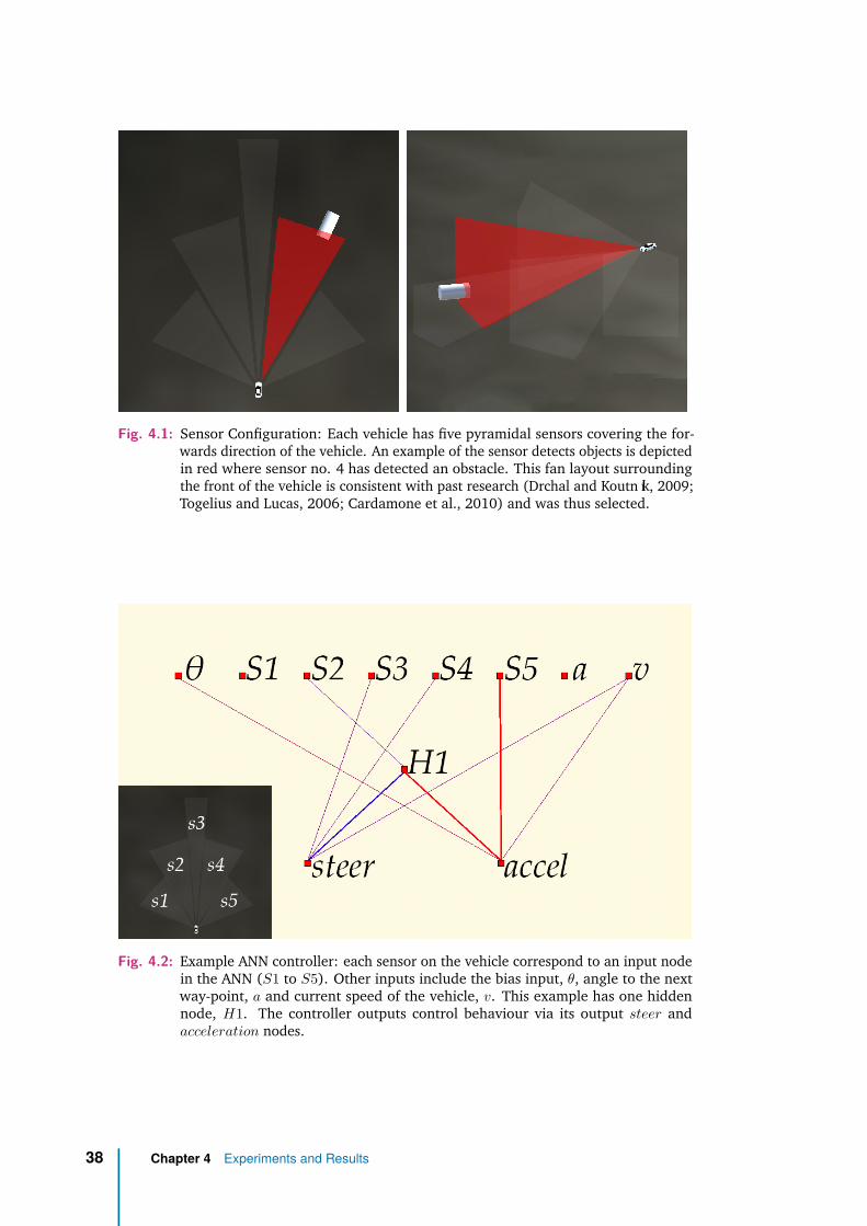
Fig. 4.1: Sensor Configuration: Each vehicle has five pyramidal sensors covering the for-wards direction of the vehicle. An example of the sensor detects objects is depictedin red where sensor no. 4 has detected an obstacle. This fan layout surroundingthe front of the vehicle is consistent with past research (Drchal and Koutník, 2009;Togelius and Lucas, 2006; Cardamone et al., 2010) and was thus selected.

Fig. 4.2: Example ANN controller: each sensor on the vehicle correspond to an input nodein the ANN (S1 to S5). Other inputs include the bias input, θ, angle to the nextway-point, a and current speed of the vehicle, v. This example has one hiddennode, H1. The controller outputs control behaviour via its output steer andacceleration nodes.

38 Chapter 4 Experiments and Results

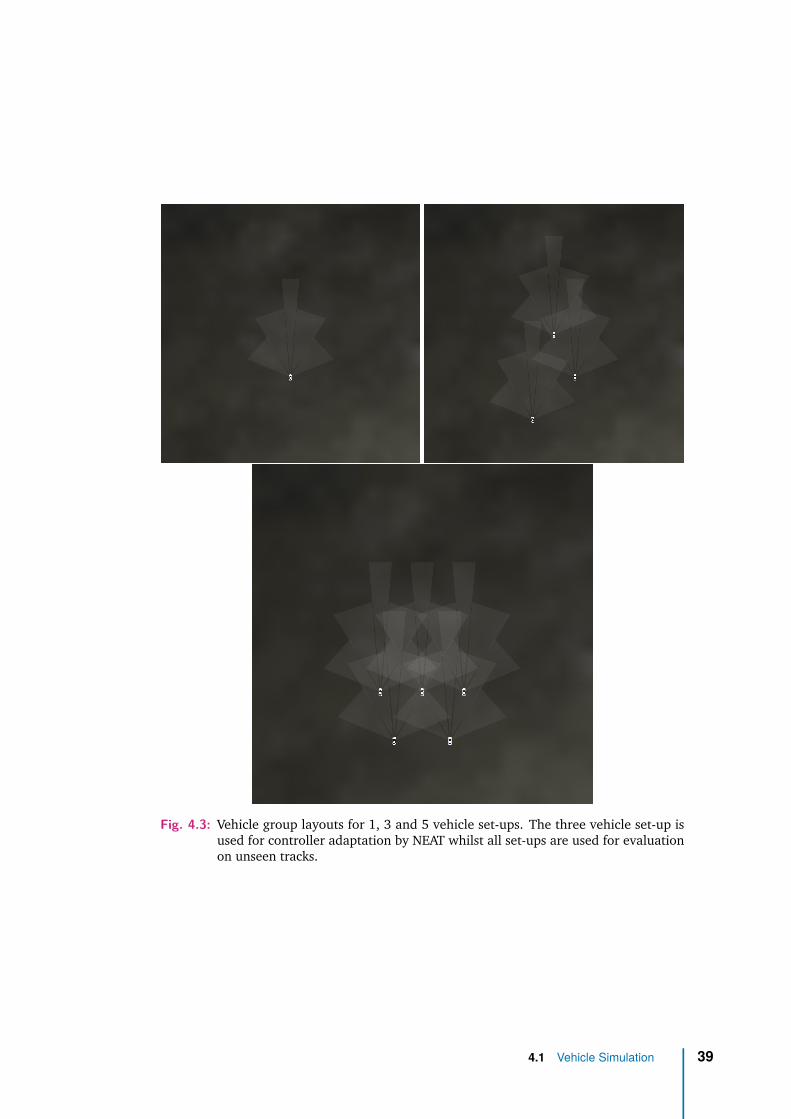
Fig. 4.3: Vehicle group layouts for 1, 3 and 5 vehicle set-ups. The three vehicle set-up isused for controller adaptation by NEAT whilst all set-ups are used for evaluationon unseen tracks.

4.1 Vehicle Simulation 39

Parameter Value

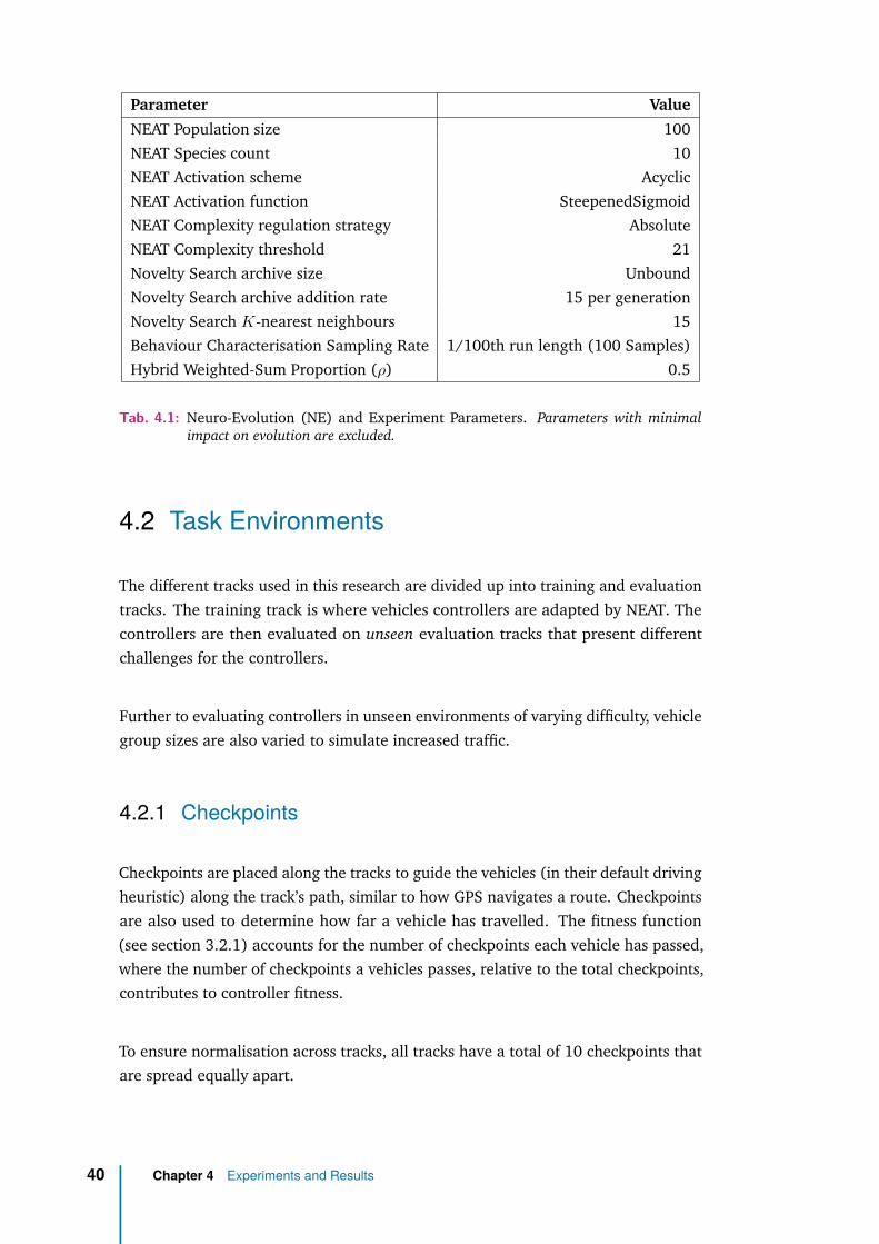
NEAT Population size 100NEAT Species count 10NEAT Activation scheme AcyclicNEAT Activation function SteepenedSigmoidNEAT Complexity regulation strategy AbsoluteNEAT Complexity threshold 21Novelty Search archive size UnboundNovelty Search archive addition rate 15 per generationNovelty Search K-nearest neighbours 15Behaviour Characterisation Sampling Rate 1/100th run length (100 Samples)Hybrid Weighted-Sum Proportion (ρ) 0.5

Tab. 4.1: Neuro-Evolution (NE) and Experiment Parameters. Parameters with minimalimpact on evolution are excluded.

4.2 Task Environments

The different tracks used in this research are divided up into training and evaluationtracks. The training track is where vehicles controllers are adapted by NEAT. Thecontrollers are then evaluated on unseen evaluation tracks that present differentchallenges for the controllers.

Further to evaluating controllers in unseen environments of varying difficulty, vehiclegroup sizes are also varied to simulate increased traffic.

4.2.1 Checkpoints

Checkpoints are placed along the tracks to guide the vehicles (in their default drivingheuristic) along the track’s path, similar to how GPS navigates a route. Checkpointsare also used to determine how far a vehicle has travelled. The fitness function(see section 3.2.1) accounts for the number of checkpoints each vehicle has passed,where the number of checkpoints a vehicles passes, relative to the total checkpoints,contributes to controller fitness.

To ensure normalisation across tracks, all tracks have a total of 10 checkpoints thatare spread equally apart.


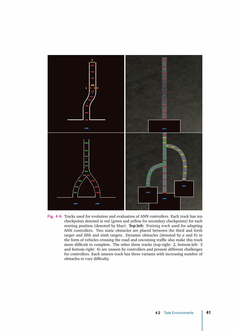
Fig. 4.4: Tracks used for evolution and evaluation of ANN controllers. Each track has tencheckpoints denoted in red (green and yellow for secondary checkpoints) for eachstarting position (denoted by blue). Top-left: Training track used for adaptingANN controllers. Two static obstacles are placed between the third and forthtarget and fifth and sixth targets. Dynamic obstacles (denoted by a and b) inthe form of vehicles crossing the road and oncoming traffic also make this trackmore difficult to complete. The other three tracks (top-right: 2, bottom-left: 3and bottom-right: 4) are unseen by controllers and present different challengesfor controllers. Each unseen track has three variants with increasing number ofobstacles to vary difficulty.

4.2 Task Environments 41

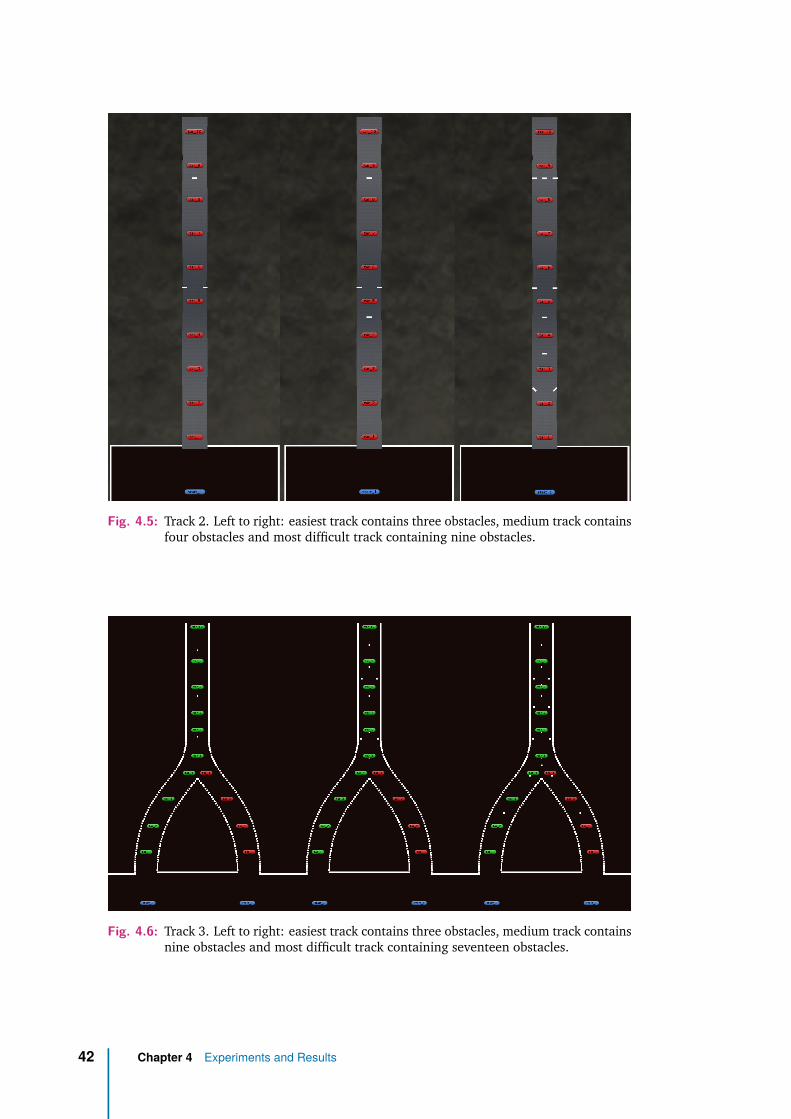
Fig. 4.5: Track 2. Left to right: easiest track contains three obstacles, medium track containsfour obstacles and most difficult track containing nine obstacles.

Fig. 4.6: Track 3. Left to right: easiest track contains three obstacles, medium track containsnine obstacles and most difficult track containing seventeen obstacles.


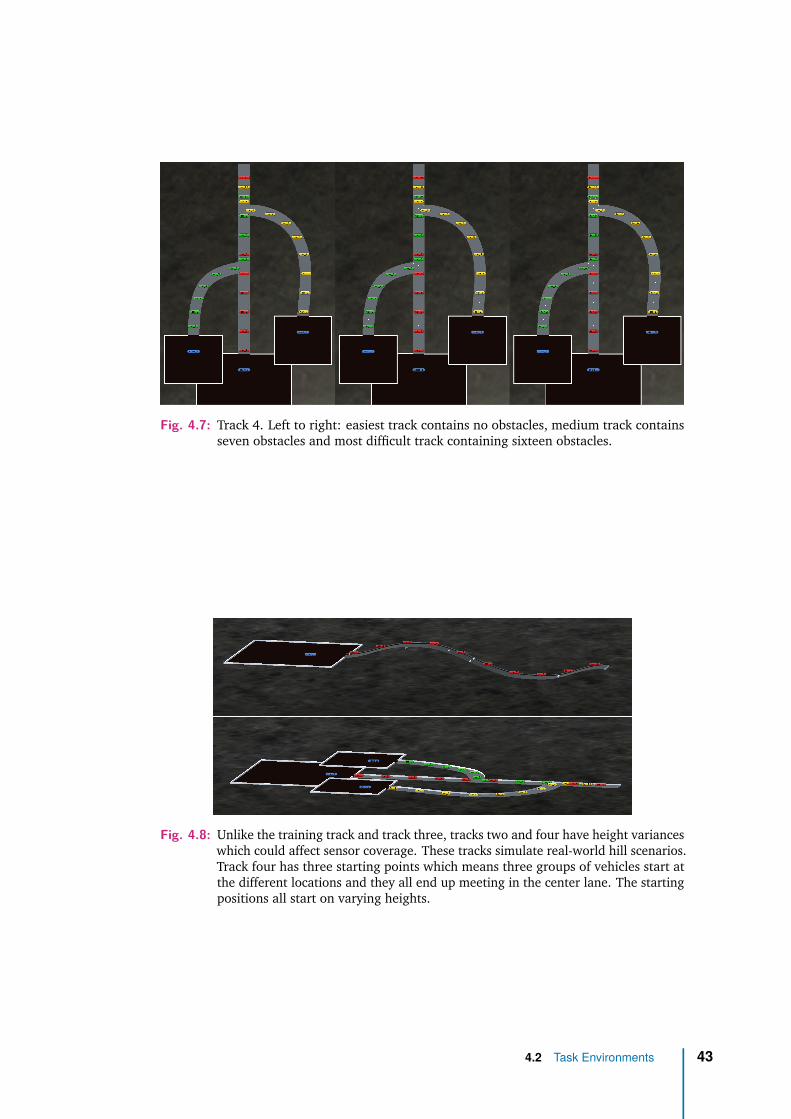
Fig. 4.7: Track 4. Left to right: easiest track contains no obstacles, medium track containsseven obstacles and most difficult track containing sixteen obstacles.

Fig. 4.8: Unlike the training track and track three, tracks two and four have height varianceswhich could affect sensor coverage. These tracks simulate real-world hill scenarios.Track four has three starting points which means three groups of vehicles start atthe different locations and they all end up meeting in the center lane. The startingpositions all start on varying heights.

4.2 Task Environments 43

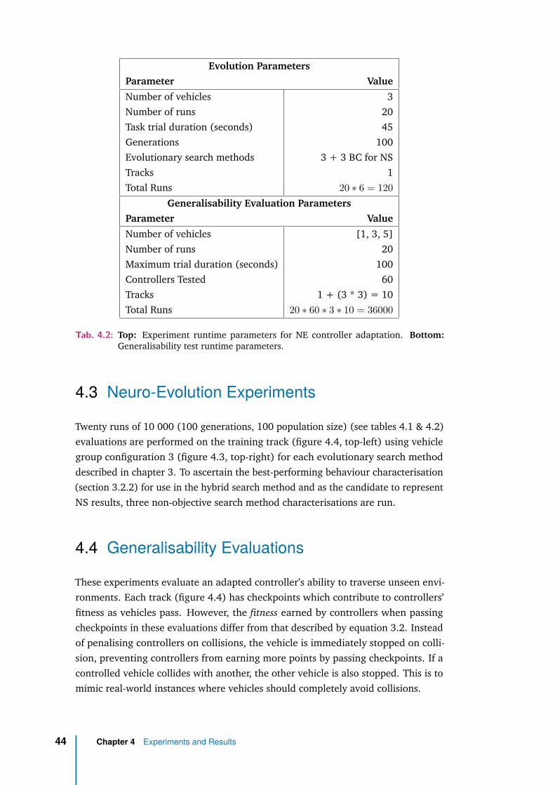
Evolution ParametersParameter Value

Number of vehicles 3Number of runs 20Task trial duration (seconds) 45Generations 100Evolutionary search methods 3 + 3 BC for NSTracks 1Total Runs 20 ∗ 6 = 120

Generalisability Evaluation ParametersParameter Value

Number of vehicles [1, 3, 5]Number of runs 20Maximum trial duration (seconds) 100Controllers Tested 60Tracks 1 + (3 * 3) = 10Total Runs 20 ∗ 60 ∗ 3 ∗ 10 = 36000

Tab. 4.2: Top: Experiment runtime parameters for NE controller adaptation. Bottom:Generalisability test runtime parameters.

4.3 Neuro-Evolution Experiments

Twenty runs of 10 000 (100 generations, 100 population size) (see tables 4.1 & 4.2)evaluations are performed on the training track (figure 4.4, top-left) using vehiclegroup configuration 3 (figure 4.3, top-right) for each evolutionary search methoddescribed in chapter 3. To ascertain the best-performing behaviour characterisation(section 3.2.2) for use in the hybrid search method and as the candidate to representNS results, three non-objective search method characterisations are run.

4.4 Generalisability Evaluations

These experiments evaluate an adapted controller’s ability to traverse unseen envi-ronments. Each track (figure 4.4) has checkpoints which contribute to controllers’fitness as vehicles pass. However, the fitness earned by controllers when passingcheckpoints in these evaluations differ from that described by equation 3.2. Insteadof penalising controllers on collisions, the vehicle is immediately stopped on colli-sion, preventing controllers from earning more points by passing checkpoints. If acontrolled vehicle collides with another, the other vehicle is also stopped. This is tomimic real-world instances where vehicles should completely avoid collisions.


Given that the fitness measurement differs in these experiments, the original trainingtrack is included here so that results can be fairly compared with unseen tracks.Table 4.3 outlines all the generalisability experiments that will be run. Since eachevolutionary search method produces twenty champions, each evaluation will berun sixty times as described in table 4.2.

4.5 Results

Overall experimental results are discussed in the proceeding section. Neuro-EvolutionResults including results behaviour characterisation tests for NS are first presented,followed by controller generalisability results. Objective-based search refers to thesearch method utilizing the only the fitness function. Non-objective refers to the NSsearch method and hybrid refers to the combination of both. Refer to section 3.2 formore information on each.

4.5.1 Neuro-Evolution (NE) Results

Three behaviour characterisations (see 3.2.2) were tested for the non-objective NSsearch method. The best-performing was selected to be the candidate to representthe non-objective search method and to be implemented for the hybrid search. Thus,these results will be presented and discussed first before a comparison is madebetween objective, non-objective and hybrid results.

Behaviour Characterisation Comparison

Results from NE controller adaptation comparing the three behaviour characteri-sations speed, speed & cohesion and location indicate that there was no statisticalsignificant difference between them (see figure 4.9). Thus, speed was selected forcomparison between the other search methods and for use in the hybrid methodsince it had the highest mean fitness overall. A simpler version of the training track(figure 4.4 top-left) was utilized for these these experiments (namely, the obstaclebetween target 3 and target 4 removed).

Overall NE Results

Results from NE controller adaptation comparing the three search methodologies,objective (fitness), non-objective (NS) and hybrid show that there was a statistical

4.5 Results 45

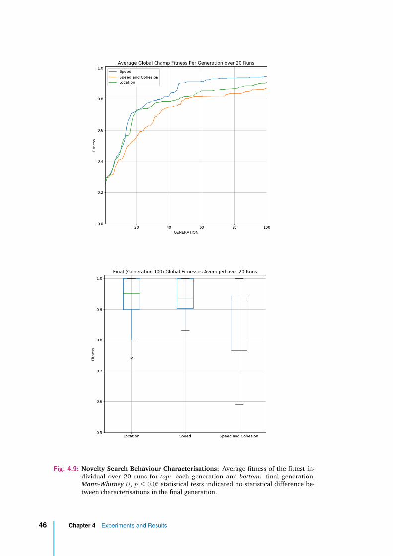
Fig. 4.9: Novelty Search Behaviour Characterisations: Average fitness of the fittest in-dividual over 20 runs for top: each generation and bottom: final generation.Mann-Whitney U, p ≤ 0.05 statistical tests indicated no statistical difference be-tween characterisations in the final generation.


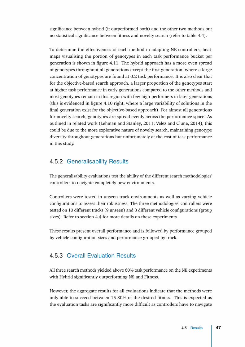
significance between hybrid (it outperformed both) and the other two methods butno statistical significance between fitness and novelty search (refer to table 4.4).

To determine the effectiveness of each method in adapting NE controllers, heat-maps visualising the portion of genotypes in each task performance bucket pergeneration is shown in figure 4.11. The hybrid approach has a more even spreadof genotypes throughout all generations except the first generation, where a largeconcentration of genotypes are found at 0.2 task performance. It is also clear thatfor the objective-based search approach, a larger proportion of the genotypes startat higher task performance in early generations compared to the other methods andmost genotypes remain in this region with few high-performers in later generations(this is evidenced in figure 4.10 right, where a large variability of solutions in thefinal generation exist for the objective-based approach). For almost all generationsfor novelty search, genotypes are spread evenly across the performance space. Asoutlined in related work (Lehman and Stanley, 2011; Velez and Clune, 2014), thiscould be due to the more explorative nature of novelty search, maintaining genotypediversity throughout generations but unfortunately at the cost of task performancein this study.

4.5.2 Generalisability Results

The generalisability evaluations test the ability of the different search methodologies’controllers to navigate completely new environments.

Controllers were tested in unseen track environments as well as varying vehicleconfigurations to assess their robustness. The three methodologies’ controllers weretested on 10 different tracks (9 unseen) and 3 different vehicle configurations (groupsizes). Refer to section 4.4 for more details on these experiments.

These results present overall performance and is followed by performance groupedby vehicle configuration sizes and performance grouped by track.

4.5.3 Overall Evaluation Results

All three search methods yielded above 60% task performance on the NE experimentswith Hybrid significantly outperforming NS and Fitness.

However, the aggregate results for all evaluations indicate that the methods wereonly able to succeed between 15-30% of the desired fitness. This is expected asthe evaluation tasks are significantly more difficult as controllers have to navigate

4.5 Results 47

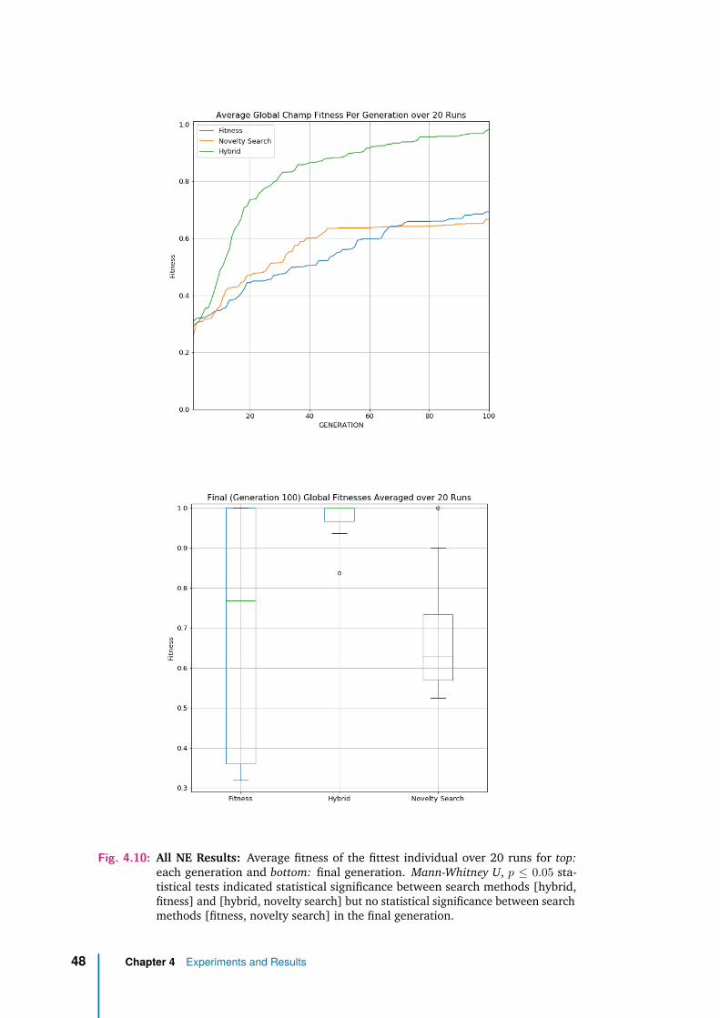
Fig. 4.10: All NE Results: Average fitness of the fittest individual over 20 runs for top:each generation and bottom: final generation. Mann-Whitney U, p ≤ 0.05 sta-tistical tests indicated statistical significance between search methods [hybrid,fitness] and [hybrid, novelty search] but no statistical significance between searchmethods [fitness, novelty search] in the final generation.


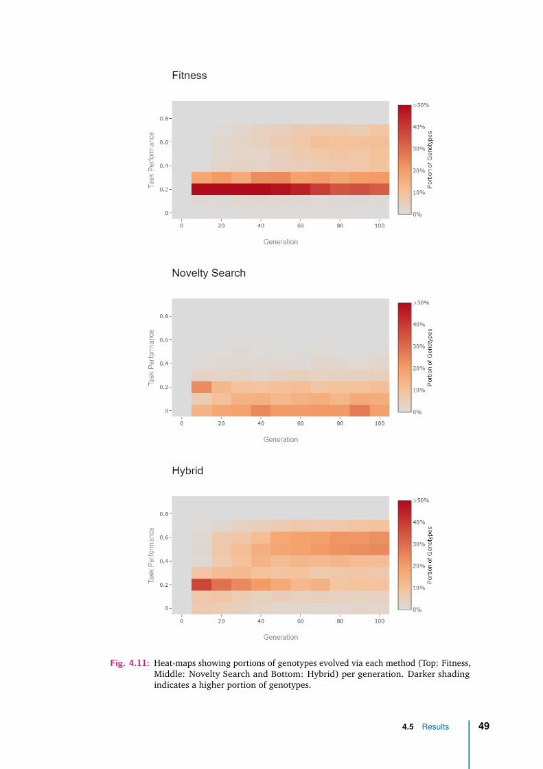
Fig. 4.11: Heat-maps showing portions of genotypes evolved via each method (Top: Fitness,Middle: Novelty Search and Bottom: Hybrid) per generation. Darker shadingindicates a higher portion of genotypes.

4.5 Results 49

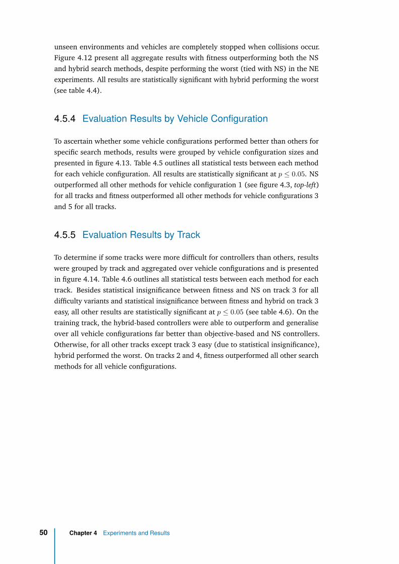
unseen environments and vehicles are completely stopped when collisions occur.Figure 4.12 present all aggregate results with fitness outperforming both the NSand hybrid search methods, despite performing the worst (tied with NS) in the NEexperiments. All results are statistically significant with hybrid performing the worst(see table 4.4).

4.5.4 Evaluation Results by Vehicle Configuration

To ascertain whether some vehicle configurations performed better than others forspecific search methods, results were grouped by vehicle configuration sizes andpresented in figure 4.13. Table 4.5 outlines all statistical tests between each methodfor each vehicle configuration. All results are statistically significant at p ≤ 0.05. NSoutperformed all other methods for vehicle configuration 1 (see figure 4.3, top-left)for all tracks and fitness outperformed all other methods for vehicle configurations 3and 5 for all tracks.

4.5.5 Evaluation Results by Track

To determine if some tracks were more difficult for controllers than others, resultswere grouped by track and aggregated over vehicle configurations and is presentedin figure 4.14. Table 4.6 outlines all statistical tests between each method for eachtrack. Besides statistical insignificance between fitness and NS on track 3 for alldifficulty variants and statistical insignificance between fitness and hybrid on track 3easy, all other results are statistically significant at p ≤ 0.05 (see table 4.6). On thetraining track, the hybrid-based controllers were able to outperform and generaliseover all vehicle configurations far better than objective-based and NS controllers.Otherwise, for all other tracks except track 3 easy (due to statistical insignificance),hybrid performed the worst. On tracks 2 and 4, fitness outperformed all other searchmethods for all vehicle configurations.


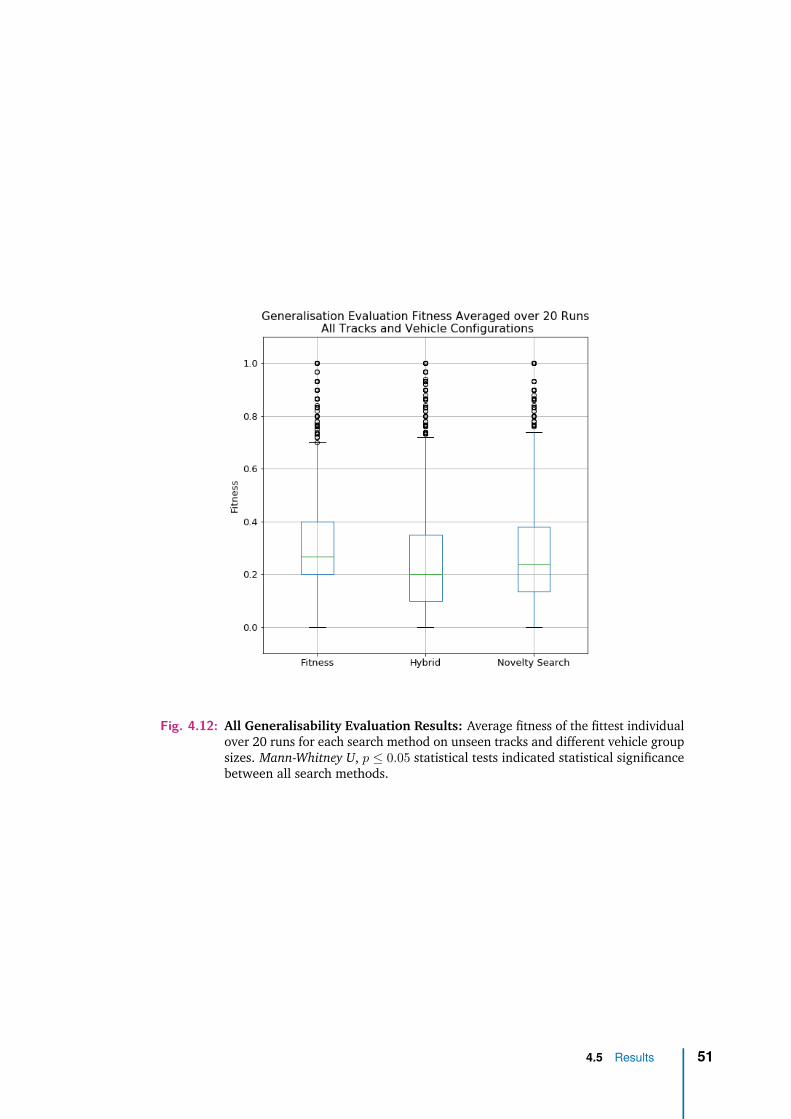
Fig. 4.12: All Generalisability Evaluation Results: Average fitness of the fittest individualover 20 runs for each search method on unseen tracks and different vehicle groupsizes. Mann-Whitney U, p ≤ 0.05 statistical tests indicated statistical significancebetween all search methods.

4.5 Results 51

Fig. 4.13: Generalisability Evaluation Results per Vehicle Configuration: Average fit-ness of the fittest individual over 20 runs for each search method on unseentracks grouped by vehicle group sizes.


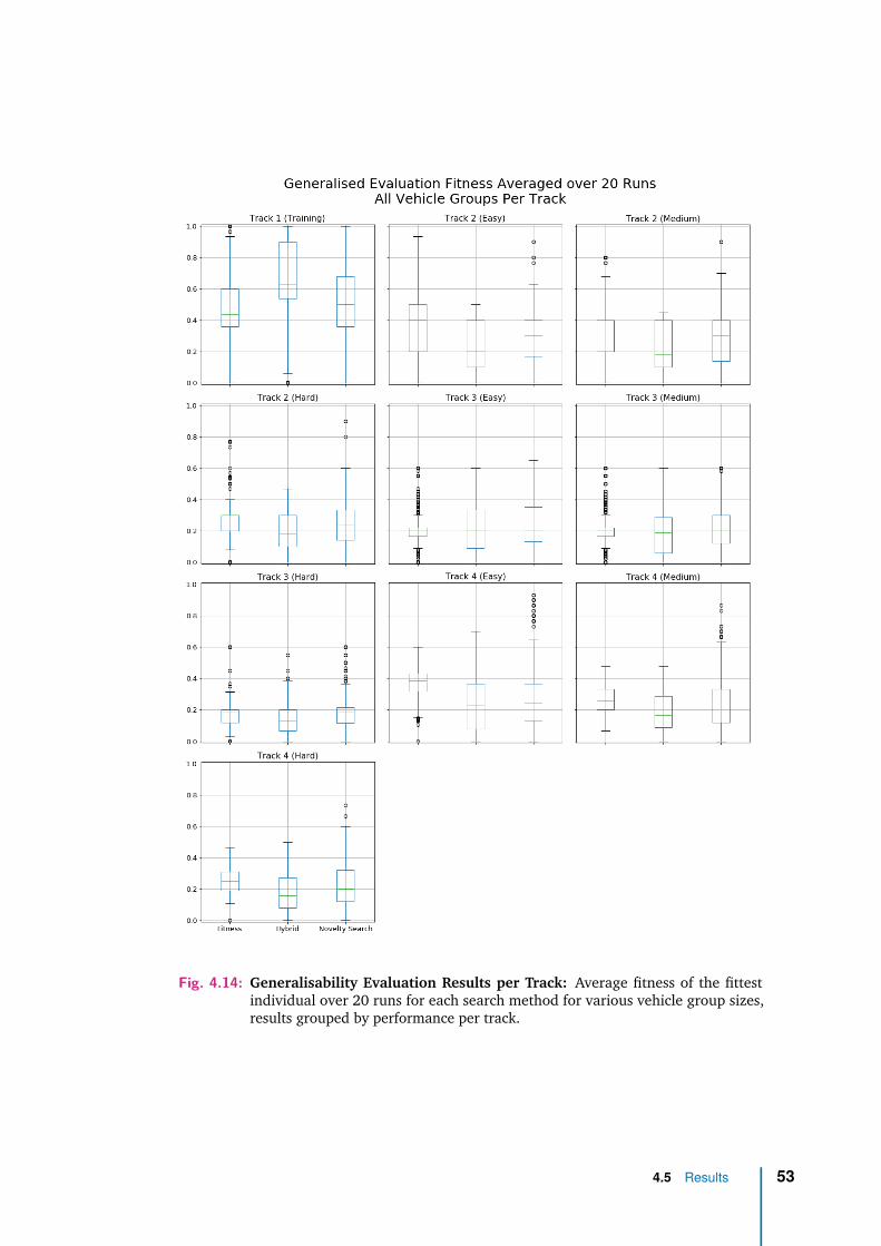
Fig. 4.14: Generalisability Evaluation Results per Track: Average fitness of the fittestindividual over 20 runs for each search method for various vehicle group sizes,results grouped by performance per track.

4.5 Results 53

Track Difficulty Variant Cars Trials

Training (Track 1) N/A 1 20Training (Track 1) - same as evolution N/A 3 20Training (Track 1) N/A 5 20

Track 2 Easy 1 20Track 2 Medium 1 20Track 2 Hard 1 20Track 2 Easy 3 20Track 2 Medium 3 20Track 2 Hard 3 20Track 2 Easy 5 20Track 2 Medium 5 20Track 2 Hard 5 20



Tab. 4.3: Schedule of Generalisability Experiments: Each of the listed experiments arerun for all sixty controllers from the three evolutionary search methods.


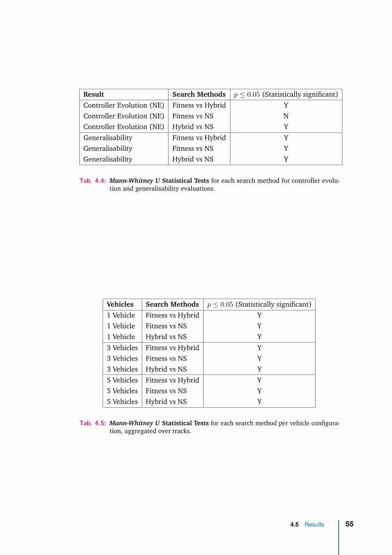
Result Search Methods p ≤ 0.05 (Statistically significant)

Controller Evolution (NE) Fitness vs Hybrid YController Evolution (NE) Fitness vs NS NController Evolution (NE) Hybrid vs NS Y

Generalisability Fitness vs Hybrid YGeneralisability Fitness vs NS YGeneralisability Hybrid vs NS Y

Tab. 4.4: Mann-Whitney U Statistical Tests for each search method for controller evolu-tion and generalisability evaluations.

Vehicles Search Methods p ≤ 0.05 (Statistically significant)

1 Vehicle Fitness vs Hybrid Y1 Vehicle Fitness vs NS Y1 Vehicle Hybrid vs NS Y

3 Vehicles Fitness vs Hybrid Y3 Vehicles Fitness vs NS Y3 Vehicles Hybrid vs NS Y

5 Vehicles Fitness vs Hybrid Y5 Vehicles Fitness vs NS Y5 Vehicles Hybrid vs NS Y

Tab. 4.5: Mann-Whitney U Statistical Tests for each search method per vehicle configura-tion, aggregated over tracks.

4.5 Results 55

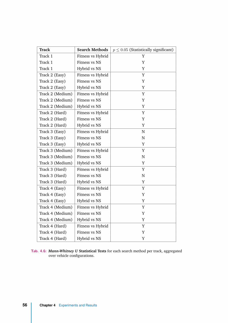
Track Search Methods p ≤ 0.05 (Statistically significant)

Track 1 Fitness vs Hybrid YTrack 1 Fitness vs NS YTrack 1 Hybrid vs NS Y

Track 2 (Easy) Fitness vs Hybrid YTrack 2 (Easy) Fitness vs NS YTrack 2 (Easy) Hybrid vs NS Y

Track 2 (Medium) Fitness vs Hybrid YTrack 2 (Medium) Fitness vs NS YTrack 2 (Medium) Hybrid vs NS Y

Track 2 (Hard) Fitness vs Hybrid YTrack 2 (Hard) Fitness vs NS YTrack 2 (Hard) Hybrid vs NS Y

Track 3 (Easy) Fitness vs Hybrid NTrack 3 (Easy) Fitness vs NS NTrack 3 (Easy) Hybrid vs NS Y

Track 3 (Medium) Fitness vs Hybrid YTrack 3 (Medium) Fitness vs NS NTrack 3 (Medium) Hybrid vs NS Y

Track 3 (Hard) Fitness vs Hybrid YTrack 3 (Hard) Fitness vs NS NTrack 3 (Hard) Hybrid vs NS Y

Track 4 (Easy) Fitness vs Hybrid YTrack 4 (Easy) Fitness vs NS YTrack 4 (Easy) Hybrid vs NS Y

Track 4 (Medium) Fitness vs Hybrid YTrack 4 (Medium) Fitness vs NS YTrack 4 (Medium) Hybrid vs NS Y

Track 4 (Hard) Fitness vs Hybrid YTrack 4 (Hard) Fitness vs NS YTrack 4 (Hard) Hybrid vs NS Y

Tab. 4.6: Mann-Whitney U Statistical Tests for each search method per track, aggregatedover vehicle configurations.


5Discussion

This chapter presents a discussion of each method’s (objective, NS and hybrid)capabilities, how they balance solution space exploration and exploitation, if theywere able to produce controllers that had desired task performance and their abilityto generalise over unseen task environments.

A detailed analysis of each along with evolved controller complexity is presentedto show how it compared with the literature where hybrid approaches are moresuitable at adapting controllers with desired task performance more efficiently andour original hypothesis that the hybrid approach will adapt controllers that willgeneralise more effectively across various unseen environments when compared with thepure-objective and pure-novelty methods in this collective self-driving task (see section1.3).

5.1 Evolved Task Performance

The NE experiment results showed that all search approaches investigated in thiswork were appropriate for the collective self-driving task. That is, they were able toevolve controllers capable of achieving 80% task performance given the constrainsof a population size of 100 and runs of 100 generations. Furthermore, it showed thatthe hybrid approach significantly outperformed the objective and NS approaches andwas the most suitable for adapting controllers that can yield desired task performanceat least 3 times quicker, that is, hybrid was able to achieve 80% task performanceby generation 30 whereas the other methods only reached these levels close togeneration 100 (see figure 4.10).

Although the NS approach initially outperformed the objective method (up to gener-ation 50), it stagnated in producing more effective controllers between generations50 and 90 with objective outperforming (but not statistically significantly) at aroundgeneration 70.

These results support previous research where hybrid approaches significantly out-perform pure objective or non-objective methods in both single-agent tasks (Huang

57

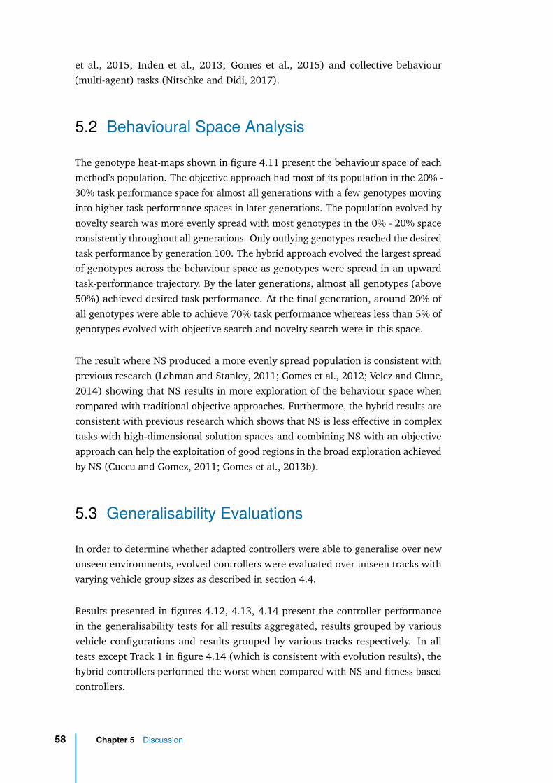
et al., 2015; Inden et al., 2013; Gomes et al., 2015) and collective behaviour(multi-agent) tasks (Nitschke and Didi, 2017).

5.2 Behavioural Space Analysis

The genotype heat-maps shown in figure 4.11 present the behaviour space of eachmethod’s population. The objective approach had most of its population in the 20% -30% task performance space for almost all generations with a few genotypes movinginto higher task performance spaces in later generations. The population evolved bynovelty search was more evenly spread with most genotypes in the 0% - 20% spaceconsistently throughout all generations. Only outlying genotypes reached the desiredtask performance by generation 100. The hybrid approach evolved the largest spreadof genotypes across the behaviour space as genotypes were spread in an upwardtask-performance trajectory. By the later generations, almost all genotypes (above50%) achieved desired task performance. At the final generation, around 20% ofall genotypes were able to achieve 70% task performance whereas less than 5% ofgenotypes evolved with objective search and novelty search were in this space.

The result where NS produced a more evenly spread population is consistent withprevious research (Lehman and Stanley, 2011; Gomes et al., 2012; Velez and Clune,2014) showing that NS results in more exploration of the behaviour space whencompared with traditional objective approaches. Furthermore, the hybrid results areconsistent with previous research which shows that NS is less effective in complextasks with high-dimensional solution spaces and combining NS with an objectiveapproach can help the exploitation of good regions in the broad exploration achievedby NS (Cuccu and Gomez, 2011; Gomes et al., 2013b).

5.3 Generalisability Evaluations

In order to determine whether adapted controllers were able to generalise over newunseen environments, evolved controllers were evaluated over unseen tracks withvarying vehicle group sizes as described in section 4.4.

Results presented in figures 4.12, 4.13, 4.14 present the controller performancein the generalisability tests for all results aggregated, results grouped by variousvehicle configurations and results grouped by various tracks respectively. In alltests except Track 1 in figure 4.14 (which is consistent with evolution results), thehybrid controllers performed the worst when compared with NS and fitness basedcontrollers.

58 Chapter 5 Discussion

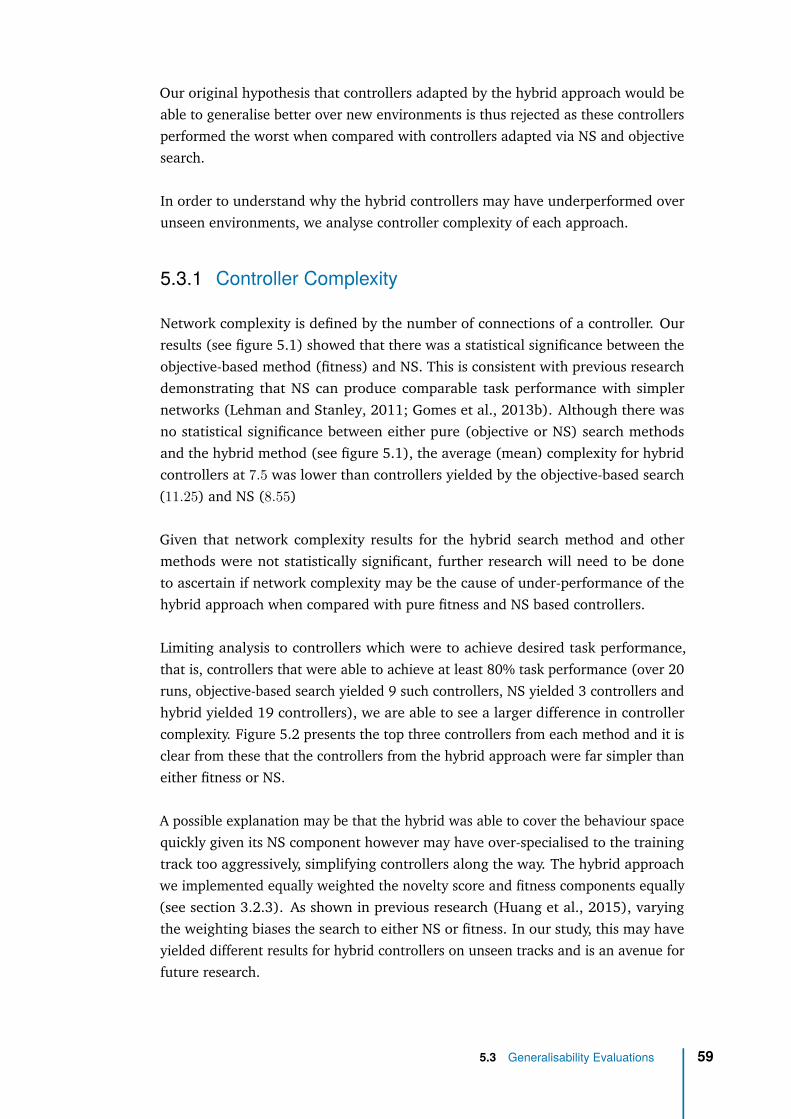
Our original hypothesis that controllers adapted by the hybrid approach would beable to generalise better over new environments is thus rejected as these controllersperformed the worst when compared with controllers adapted via NS and objectivesearch.

In order to understand why the hybrid controllers may have underperformed overunseen environments, we analyse controller complexity of each approach.

5.3.1 Controller Complexity

Network complexity is defined by the number of connections of a controller. Ourresults (see figure 5.1) showed that there was a statistical significance between theobjective-based method (fitness) and NS. This is consistent with previous researchdemonstrating that NS can produce comparable task performance with simplernetworks (Lehman and Stanley, 2011; Gomes et al., 2013b). Although there wasno statistical significance between either pure (objective or NS) search methodsand the hybrid method (see figure 5.1), the average (mean) complexity for hybridcontrollers at 7.5 was lower than controllers yielded by the objective-based search(11.25) and NS (8.55)

Given that network complexity results for the hybrid search method and othermethods were not statistically significant, further research will need to be doneto ascertain if network complexity may be the cause of under-performance of thehybrid approach when compared with pure fitness and NS based controllers.

Limiting analysis to controllers which were to achieve desired task performance,that is, controllers that were able to achieve at least 80% task performance (over 20runs, objective-based search yielded 9 such controllers, NS yielded 3 controllers andhybrid yielded 19 controllers), we are able to see a larger difference in controllercomplexity. Figure 5.2 presents the top three controllers from each method and it isclear from these that the controllers from the hybrid approach were far simpler thaneither fitness or NS.

A possible explanation may be that the hybrid was able to cover the behaviour spacequickly given its NS component however may have over-specialised to the trainingtrack too aggressively, simplifying controllers along the way. The hybrid approachwe implemented equally weighted the novelty score and fitness components equally(see section 3.2.3). As shown in previous research (Huang et al., 2015), varyingthe weighting biases the search to either NS or fitness. In our study, this may haveyielded different results for hybrid controllers on unseen tracks and is an avenue forfuture research.

5.3 Generalisability Evaluations 59

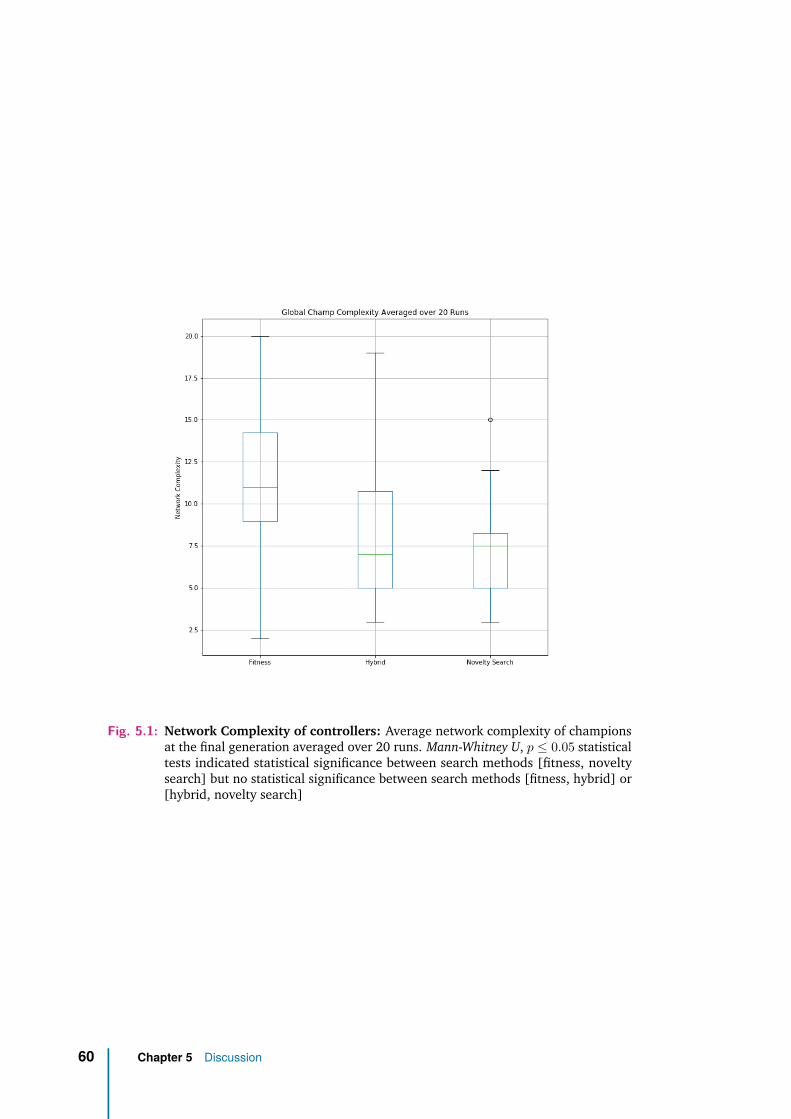
Fig. 5.1: Network Complexity of controllers: Average network complexity of championsat the final generation averaged over 20 runs. Mann-Whitney U, p ≤ 0.05 statisticaltests indicated statistical significance between search methods [fitness, noveltysearch] but no statistical significance between search methods [fitness, hybrid] or[hybrid, novelty search]

60 Chapter 5 Discussion

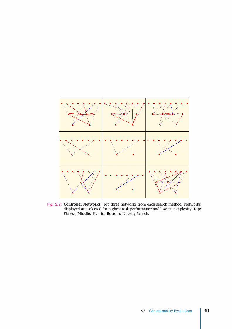
Fig. 5.2: Controller Networks: Top three networks from each search method. Networksdisplayed are selected for highest task performance and lowest complexity. Top:Fitness, Middle: Hybrid. Bottom: Novelty Search.

5.3 Generalisability Evaluations 61

6Conclusion

This final chapter summarises our findings and how they relate to our originalhypothesis and concludes with known limitations and future work.

6.1 Summary of Findings and Results

This work aimed at applying Neuro-Evolution (NE) to the collective self-driving task(chapter 4), an area of vast scientific and commercial interest as it may present thenext frontier of personal transportation systems.

We examined three different search methodologies for a popular and well-researchedNE framework, NEAT. Our research supported previous work with consistent resultswhere hybrid approaches are able to outperform pure objective and NS approachesin terms of task performance and evolution speed.

Furthermore, we presented generalisability experiments that aimed at contributingto the literature in terms of showing how each approach, Objective-based, NS andHybrid perform on unseen task environments. Based on related work (Huang et al.,2015; Inden et al., 2013; Cuccu and Gomez, 2011), our hypothesis was that thehybrid approach will not only outperform both pure approaches in the training task,but also unseen tasks.

However, our results did not support this hypothesis and hybrid ultimately wereoutperformed by objective-based search and NS. This result contrasted the hybridmethod’s ability to outperform pure objective-based and NS methods, highlightinghybrid’s inability to generalise to unseen environments.

6.2 Known Limitations

The track widths in the simulator were significantly wider than real-world roads.Each tracks’ width was at least 15 vehicles wide which is unrealistic. This was dueto controllers unable to adapt when track widths were narrower which would causesensors to detect obstacles constantly.

63

Sensors also did not distinguish between detected object types. All objects that itdetected (walls, static obstacles, other vehicles in its group, dynamic obstacles) wereall treated the same way.

Since the unity game engine produces a physically realistic simulation, randomnessis part of the simulation and our NE task trials were only run once per genotypeper generation. This means that randomness could cause some genotypes to havehigher fitness than others in the NE adaptation phase which we did not average overmultiple runs (this was done in the evaluations, however).

6.3 Future Work

Given our simple (equal weighting) implementation of our hybrid approach, testingvarious degrees of weighting between fitness and novelty may yield significantlydifferent results.

Improving the simulator with sensors which consider object types and narrowerroads could also affect task performance and adapting controllers on more than justone track and varying the environment or vehicle sizes could possibly yield differentresults since the given track may have biased a specific search methodology.

Implementing the three different approaches in related collective behaviour tasks(such as, swarm robotics) may yield different results, especially our result wherehybrid doesn’t generalise over a range of unknown tasks and may indicate domain-specific reasons relating to poor task generalisability.

Finally, given our observed results, introducing a more robust evolution (training)track by introducing more noise (beyond traffic randomness) during evolution mayyield different results by mitigating the risk of the various search approaches tooverspecialising to the training track.

64 Chapter 6 Conclusion

Bibliography

Angeline, Peter J, Gregory M Saunders, and Jordan B Pollack (1994). „An evolutionaryalgorithm that constructs recurrent neural networks“. In: IEEE transactions on NeuralNetworks 5.1, pp. 54–65 (cit. on p. 15).

Applegate, David L, Robert E Bixby, Vasek Chvatal, and William J Cook (2006). The travelingsalesman problem: a computational study. Princeton university press (cit. on p. 11).

Bahdanau, Dzmitry, Kyunghyun Cho, and Yoshua Bengio (2014). „Neural machine translationby jointly learning to align and translate“. In: arXiv preprint arXiv:1409.0473 (cit. on p. 9).

Baldi, Pierre (1995). „Gradient descent learning algorithm overview: A general dynamicalsystems perspective“. In: IEEE Transactions on Neural Networks 6.1, pp. 182–195 (cit. onp. 9).

Bamonte, T. (2013). „Autonomous Vehicles: Drivers for Change“. In: Roads and BridgesSummer, pp. 5–10 (cit. on p. 25).

Beeson, Patrick, Jack O’Quin, Bartley Gillan, et al. (2008). „Multiagent Interactions in UrbanDriving“. In: Journal of Physical Agents 2.1. Special issue on Multi-Robot Systems, pp. 15–30 (cit. on p. 25).

Beni, G. (2004). „From Swarm Intelligence to Swarm Robotics“. In: Proceedings of theInternational Workshop on Swarm Robotics, pp. 1–9 (cit. on p. 27).

Bilger, B. (2013). „Auto Correct: Has The Self-Driving Car At Last Arrived“. In: New Yorker25 November (cit. on p. 25).

Bryant, Bobby D and Risto Miikkulainen (2003). „Neuroevolution for adaptive teams“. In:Evolutionary Computation, 2003. CEC’03. The 2003 Congress on. Vol. 3. IEEE, pp. 2194–2201 (cit. on p. 3).

Cardamone, Luigi, Daniele Loiacono, and Pier Luca Lanzi (2010). „Learning to drive in theopen racing car simulator using online neuroevolution“. In: Computational Intelligenceand AI in Games, IEEE Transactions on 2.3, pp. 176–190 (cit. on pp. 20, 25–27, 38).

Ciregan, Dan, Ueli Meier, and Jürgen Schmidhuber (2012). „Multi-column deep neuralnetworks for image classification“. In: Computer Vision and Pattern Recognition (CVPR),2012 IEEE Conference on. IEEE, pp. 3642–3649 (cit. on p. 9).

Clune, Jeff, Kenneth O Stanley, Robert T Pennock, and Charles Ofria (2011). „On theperformance of indirect encoding across the continuum of regularity“. In: IEEE Transactionson Evolutionary Computation 15.3, pp. 346–367 (cit. on p. 12).

65

Cuccu, G. and F. Gomez (2011). „When novelty is not enough“. In: Applications of Evolution-ary Computation. Springer, pp. 234–243 (cit. on pp. 24, 25, 58, 63).

Drchal, Jan, Jan Koutník, et al. (2009). „HyperNEAT controlled robots learn how to driveon roads in simulated environment“. In: Evolutionary Computation, 2009. CEC’09. IEEECongress on Evolutionary Computation. IEEE, pp. 1087–1092 (cit. on pp. 3, 25–27, 38).

Ebner, M. and T. Tiede (2009). „Evolving driving controllers using Genetic Programming“.In: Proceedings of the IEEE Symposium on Computational Intelligence and Games. Milano,Italy: IEEE Press, pp. 279–286 (cit. on pp. 3, 25–27).

Eiben, Agoston E and James E Smith (2003). Introduction to evolutionary computing. SpringerScience & Business Media (cit. on pp. 10, 11).

Floreano, Dario and Claudio Mattiussi (2008). Bio-inspired artificial intelligence: theories,methods, and technologies. MIT press (cit. on p. 3).

Fogel, David B and Lawrence J Fogel (1995). „An introduction to evolutionary programming“.In: European Conference on Artificial Evolution. Springer, pp. 21–33 (cit. on p. 10).

Furda, Andrei and Ljubo Vlacic (2011). „Enabling safe autonomous driving in real-worldcity traffic using multiple criteria decision making“. In: Intelligent Transportation SystemsMagazine, IEEE 3.1, pp. 4–17 (cit. on p. 25).

Goldberg, David E and John H Holland (1988). „Genetic algorithms and machine learning“.In: Machine learning 3.2, pp. 95–99 (cit. on p. 10).

Gomes, Jorge, Paulo Urbano, and Anders Lyhne Christensen (2012). „Introducing noveltysearch in evolutionary swarm robotics“. In: International Conference on Swarm Intelligence.Springer, pp. 85–96 (cit. on p. 58).

– (Jan. 1, 2013a). „Evolution of swarm robotics systems with novelty search“. In: SwarmIntelligence 7.2–3, pp. 115–144. published (cit. on p. 25).

– (2013b). „Evolution of swarm robotics systems with novelty search“. In: Swarm Intelligence7.2-3, pp. 115–144 (cit. on pp. 58, 59).

Gomes, Jorge, Pedro Mariano, and Anders Lyhne Christensen (2015). „Devising effectivenovelty search algorithms: A comprehensive empirical study“. In: Proceedings of the 2015Annual Conference on Genetic and Evolutionary Computation. ACM, pp. 943–950 (cit. onp. 58).

Gomes, Jorge, Miguel Duarte, Pedro Mariano, and Anders Lyhne Christensen (Sept. 1, 2016).„Cooperative Coevolution of Control for a Real Multirobot System“. In: Parallel ProblemSolving from Nature – PPSN XIV. Springer, pp. 591–601. published (cit. on p. 25).

Gomez, F., J. Schmidhuber, and R. Miikkulainen (2006). „Efficient non-linear control throughneuroevolution“. In: Machine Learning: European Conference on Machine Learning. Springer,pp. 654–662 (cit. on p. 3).

Gomez, Faustino and Risto Miikkulainen (1997). „Incremental evolution of complex generalbehavior“. In: Adaptive Behavior 5.3-4, pp. 317–342 (cit. on p. 13).

Gomez, Faustino, Jürgen Schmidhuber, and Risto Miikkulainen (2008). „Accelerated neuralevolution through cooperatively coevolved synapses“. In: The Journal of Machine LearningResearch 9, pp. 937–965 (cit. on pp. 12, 13, 24).

66 Bibliography

Gomez, Faustino J and Risto Miikkulainen (1999). „Solving non-Markovian control taskswith neuroevolution“. In: IJCAI. Vol. 99, pp. 1356–1361 (cit. on p. 24).

Gomez, Faustino John (2003). „Robust non-linear control through neuroevolution“. PhDthesis (cit. on pp. 7, 12, 13).

Gould, Stephen Jay (1996). „Full House: the Spread of Excellence from Plato to Darwin,1996“. In: See also excerpts of Stephen Jay Gould on Stanford Presidential Lectures in theHumanities and Arts, p. 197 (cit. on p. 21).

Gower, John Clifford (1982). „Euclidean distance geometry“. In: Math. Sci 7.1, pp. 1–14(cit. on p. 33).

Green, C (2003). SharpNEAT homepage (cit. on p. 31).

Grefenstette, John, Rajeev Gopal, Brian Rosmaita, and Dirk Van Gucht (1985). „Geneticalgorithms for the traveling salesman problem“. In: Proceedings of the first InternationalConference on Genetic Algorithms and their Applications, pp. 160–168 (cit. on p. 11).

Gruau, Frederic (1993). „Genetic synthesis of modular neural networks“. In: Proceedings ofthe 5th International Conference on Genetic Algorithms. Morgan Kaufmann Publishers Inc.,pp. 318–325 (cit. on pp. 12–15).

Huang, Chien-Lun Allen, Geoff Nitschke, and David Shorten (2015). „Searching for noveltyin pole balancing“. In: Evolutionary Computation (CEC), 2015 IEEE Congress on. IEEE,pp. 1792–1798 (cit. on pp. 3, 24, 25, 34, 35, 57, 59, 63).

Igel, Christian (2003). „Neuroevolution for reinforcement learning using evolution strate-gies“. In: The 2003 Congress on Evolutionary Computation, 2003. CEC’03. Vol. 4. IEEE,pp. 2588–2595 (cit. on p. 24).

Inden, Benjamin, Yaochu Jin, Robert Haschke, Helge Ritter, and Bernhard Sendhoff (2013).„An examination of different fitness and novelty based selection methods for the evolutionof neural networks“. In: Soft Computing 17.5, pp. 753–767 (cit. on pp. 24, 25, 58, 63).

Jallov, Daniel Ingmer (2014). „Evolve-Introducing a Novel Game Mechanic Based on theIndirect Control Of Evolving Neural Networks“. In: (cit. on pp. 20, 31).

Kenwell, Bret (2018). Will Tesla Be the First Automaker to Offer Fully-Autonomous Driving?(Cit. on p. 28).

Kesting, Arne, Martin Treiber, and Dirk Helbing (2010). „Enhanced intelligent driver modelto access the impact of driving strategies on traffic capacity“. In: Philosophical Transactionsof the Royal Society of London A: Mathematical, Physical and Engineering Sciences 368.1928,pp. 4585–4605 (cit. on p. 25).

Koza, John R (1994). „Genetic programming as a means for programming computers bynatural selection“. In: Statistics and computing 4.2, pp. 87–112 (cit. on p. 11).

KPMG, Center for Automotive Research (2012). Self-Driving Cars: The Next Revolution.https://www.kpmg.com/US/en/IssuesAndInsights/ArticlesPublications/Documents/self-driving-cars-next-revolution.pdf (cit. on p. 25).

Krishna (2018). Introduction to Exponential Linear Unit (cit. on p. 10).

Kube, R. and H. Zhang (1994). „Stagnation recovery behaviours for collective robotics“. In:IEEE/RSJ IROS. Cambridge, USA: MIT Press, pp. 1883–1890 (cit. on p. 27).

Bibliography 67

Lehman, Joel and Kenneth O Stanley (2011). „Abandoning objectives: Evolution through thesearch for novelty alone“. In: Evolutionary computation 19.2, pp. 189–223 (cit. on pp. 1,3, 21–23, 47, 58, 59).

Levinson, Jesse, Jake Askeland, Jan Becker, et al. (2011). „Towards fully autonomous driving:Systems and algorithms“. In: Intelligent Vehicles Symposium (IV), 2011 IEEE. IEEE, pp. 163–168 (cit. on p. 2).

Martinoli, A., Y. Zhang, P. Prakash, E. Antonsson, and R. Olney (2002). „Towards EvolutionaryDesign of Intelligent Transportation Systems.“ In: Eleventh International Symposium onNew Technologies for Advanced Driver Assistance Systems. Siena, Italy.: ATA Press, pp. 283–290 (cit. on p. 1).

Miconi, Thomas (2008). „Evolution and complexity: The double-edged sword“. In: Artificiallife 14.3, pp. 325–344 (cit. on p. 21).

Moriarty, David E and Risto Mikkulainen (1996). „Efficient reinforcement learning throughsymbiotic evolution“. In: Machine learning 22.1-3, pp. 11–32 (cit. on pp. 12, 13).

Motavalli, J. (2012). „Self-Driving Cars Will Take Over By 2040“. In: Forbes Magazine 25September (cit. on p. 25).

Mouret, J-B and Stéphane Doncieux (2012). „Encouraging behavioral diversity in evolution-ary robotics: An empirical study“. In: Evolutionary computation 20.1, pp. 91–133 (cit. onp. 25).

NHTSA (2016). Electronic Stability Control (ESC) (cit. on p. 28).

Nitschke, Geoff and Sabre Didi (2017). „Evolutionary policy transfer and search methods forboosting behavior quality: Robocup keep-away case study“. In: Frontiers in Robotics andAI 4, p. 62 (cit. on pp. 25, 58).

Parker, Aashiq and Geoff Nitschke (2017). „Autonomous intersection driving with neuro-evolution“. In: Proceedings of the Genetic and Evolutionary Computation Conference Com-panion. ACM, pp. 133–134 (cit. on p. 20).

Pathak, Deepak, Pulkit Agrawal, Alexei A Efros, and Trevor Darrell (2017). „Curiosity-drivenexploration by self-supervised prediction“. In: (cit. on p. 21).

Pomerleau, Dean A (1991). „Efficient training of artificial neural networks for autonomousnavigation“. In: Neural Computation 3.1, pp. 88–97 (cit. on p. 9).

Radding, Charles M (1982). „Homologous pairing and strand exchange in genetic recombi-nation“. In: Annual review of genetics 16.1, pp. 405–437 (cit. on p. 18).

Sigmund, Karl (1995). „Games of life: explorations in ecology, evolution and behavior“. In:(cit. on p. 21).

Space-Based Positioning, Navigation National Coordination Office for and Timing (2017).Roads and Highways (cit. on p. 2).

Stanley, Kenneth O and Risto Miikkulainen (2002). „Evolving neural networks throughaugmenting topologies“. In: Evolutionary computation 10.2, pp. 99–127 (cit. on pp. 1, 3,12–15, 18–20).

Stanley, Kenneth O, David B D’Ambrosio, and Jason Gauci (2009). „A hypercube-basedencoding for evolving large-scale neural networks“. In: Artificial life 15.2, pp. 185–212(cit. on p. 12).

68 Bibliography

Talamini, Jacopo, Giovanni Scaini, Eric Medvet, and Alberto Bartoli (2018). „Selfish vs.global behavior promotion in car controller evolution“. In: Proceedings of the Genetic andEvolutionary Computation Conference Companion. ACM, pp. 1722–1727 (cit. on pp. 25,26).

Togelius, J. and S. Lucas (2005). „Evolving controllers for simulated car racing“. In: Pro-ceedings of the IEEE Congress on Evolutionary Computation. Edinburgh, UK: IEEE Press,pp. 1906–1913 (cit. on p. 25).

– (2006). „Evolving robust and specialized car racing skills“. In: Proceedings of the IEEECongress on Evolutionary Computation. Vancouver, Canada: IEEE Press, pp. 1187–1194(cit. on pp. 3, 25–27, 38).

Trianni, Vito, Stefano Nolfi, and Marco Dorigo (2006). „Cooperative hole avoidance in aswarm-bot“. In: Robotics and Autonomous Systems 54.2, pp. 97–103 (cit. on p. 3).

Velez, Roby and Jeff Clune (2014). „Novelty search creates robots with general skills forexploration“. In: Proceedings of the 2014 Annual Conference on Genetic and EvolutionaryComputation. ACM, pp. 737–744 (cit. on pp. 47, 58).

Waibel, Markus, Laurent Keller, and Dario Floreano (2009). „Genetic team composition andlevel of selection in the evolution of cooperation“. In: IEEE Transactions on EvolutionaryComputation 13.3, pp. 648–660 (cit. on p. 3).

Wasef, Basem (2018). 2019 Audi A8 L Review | Brilliant engineering in an unassumingwrapper (cit. on p. 29).

Watson, J. and G. Nitschke (2015). „Evolving Robust Robot Team Morphologies for CollectiveConstruction“. In: Proceedings of the IEEE Symposium Series on Computational Intelligence,pp. 1039–1046 (cit. on pp. 20, 27).

Werfel, J. (2007). „Building Blocks for Multi-robot Construction“. In: Distributed AutonomousRobotic Systems 6. Tokyo, Japan: Springer, pp. 285–294 (cit. on p. 27).

Wieland, Alexis P (1991). „Evolving neural network controllers for unstable systems“. In:Neural Networks, 1991., IJCNN-91-Seattle International Joint Conference on. Vol. 2. IEEE,pp. 667–673 (cit. on pp. 11–13).

Willigen, Willem H van, Evert Haasdijk, and Leon JHM Kester (2013). „Evolving intelligentvehicle control using multi-objective neat“. In: Computational Intelligence in Vehicles andTransportation Systems (CIVTS), 2013 IEEE Symposium on. IEEE, pp. 9–15 (cit. on p. 20).

Woolley, Brian G and Kenneth O Stanley (2011). „On the deleterious effects of a prioriobjectives on evolution and representation“. In: Proceedings of the 13th annual conferenceon Genetic and evolutionary computation. ACM, pp. 957–964 (cit. on p. 21).

Yegnanarayana, B (2009). Artificial neural networks. PHI Learning Pvt. Ltd. (cit. on p. 9).

Zhang, Byoung-Tak and Heinz Muhlenbein (1993). „Evolving optimal neural networks usinggenetic algorithms with Occam’s razor“. In: Complex systems 7.3, pp. 199–220 (cit. onp. 16).

Zhang, Yizhen, Alcherio Martinoli, and Erik K Antonsson (2003). „Evolutionary design of acollective sensory system“. In: Proc. of the 2003 AAAI Spring Symposium on ComputationalSynthesis. SWIS-CONF-2003-007, pp. 283–290 (cit. on p. 1).

Bibliography 69

Websites

Ackerman, Evan (2015). Tesla Model S: Summer Software Update Will Enable AutonomousDriving. URL: http://spectrum.ieee.org/cars-that-think/transportation/self-driving/tesla-model-s-to-combine-safety-sensors-to-go-autonomous (visitedon Mar. 20, 2015) (cit. on p. 25).

Highway, National and Traffic Safety Administration (2013). U.S. Department of Transporta-tion Releases Policy on Automated Vehicle Development. URL: http://www.nhtsa.gov/About+NHTSA/Press+Releases/U.S.+Department+of+Transportation+Releases+Policy+on+Automated+Vehicle+Development (visited on Apr. 1, 2016) (cit. on p. 28).

70 Bibliography

http://spectrum.ieee.org/cars-that-think/transportation/self-driving/tesla-model-s-to-combine-safety-sensors-to-go-autonomous

http://spectrum.ieee.org/cars-that-think/transportation/self-driving/tesla-model-s-to-combine-safety-sensors-to-go-autonomous

http://www.nhtsa.gov/About+NHTSA/Press+Releases/U.S.+Department+of+Transportation+Releases+Policy+on+Automated+Vehicle+Development



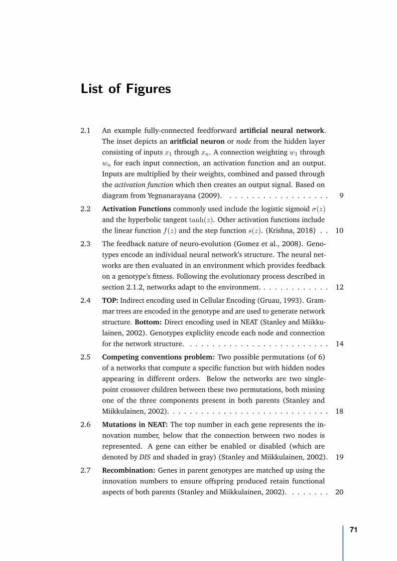
List of Figures

2.1 An example fully-connected feedforward artificial neural network.The inset depicts an aritficial neuron or node from the hidden layerconsisting of inputs x1 through xn. A connection weighting w1 throughwn for each input connection, an activation function and an output.Inputs are multiplied by their weights, combined and passed throughthe activation function which then creates an output signal. Based ondiagram from Yegnanarayana (2009). . . . . . . . . . . . . . . . . . . 9

2.2 Activation Functions commonly used include the logistic sigmoid σ(z)and the hyperbolic tangent tanh(z). Other activation functions includethe linear function f(z) and the step function s(z). (Krishna, 2018) . . 10

2.3 The feedback nature of neuro-evolution (Gomez et al., 2008). Geno-types encode an individual neural network’s structure. The neural net-works are then evaluated in an environment which provides feedbackon a genotype’s fitness. Following the evolutionary process described insection 2.1.2, networks adapt to the environment. . . . . . . . . . . . . 12

2.4 TOP: Indirect encoding used in Cellular Encoding (Gruau, 1993). Gram-mar trees are encoded in the genotype and are used to generate networkstructure. Bottom: Direct encoding used in NEAT (Stanley and Miikku-lainen, 2002). Genotypes expliclity encode each node and connectionfor the network structure. . . . . . . . . . . . . . . . . . . . . . . . . . 14

2.5 Competing conventions problem: Two possible permutations (of 6)of a networks that compute a specific function but with hidden nodesappearing in different orders. Below the networks are two single-point crossover children between these two permutations, both missingone of the three components present in both parents (Stanley andMiikkulainen, 2002). . . . . . . . . . . . . . . . . . . . . . . . . . . . . 18

2.6 Mutations in NEAT: The top number in each gene represents the in-novation number, below that the connection between two nodes isrepresented. A gene can either be enabled or disabled (which aredenoted by DIS and shaded in gray) (Stanley and Miikkulainen, 2002). 19

2.7 Recombination: Genes in parent genotypes are matched up using theinnovation numbers to ensure offspring produced retain functionalaspects of both parents (Stanley and Miikkulainen, 2002). . . . . . . . 20

71

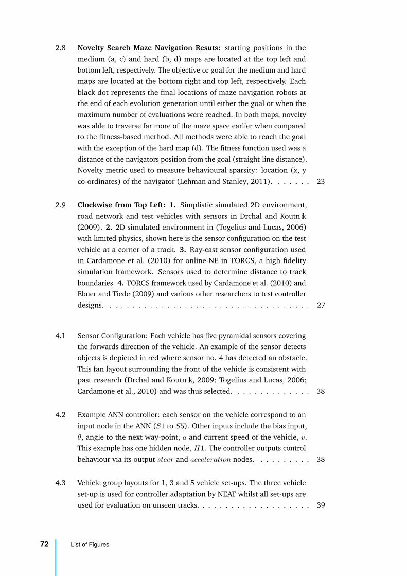
2.8 Novelty Search Maze Navigation Resuts: starting positions in themedium (a, c) and hard (b, d) maps are located at the top left andbottom left, respectively. The objective or goal for the medium and hardmaps are located at the bottom right and top left, respectively. Eachblack dot represents the final locations of maze navigation robots atthe end of each evolution generation until either the goal or when themaximum number of evaluations were reached. In both maps, noveltywas able to traverse far more of the maze space earlier when comparedto the fitness-based method. All methods were able to reach the goalwith the exception of the hard map (d). The fitness function used was adistance of the navigators position from the goal (straight-line distance).Novelty metric used to measure behavioural sparsity: location (x, yco-ordinates) of the navigator (Lehman and Stanley, 2011). . . . . . . 23

2.9 Clockwise from Top Left: 1. Simplistic simulated 2D environment,road network and test vehicles with sensors in Drchal and Koutník(2009). 2. 2D simulated environment in (Togelius and Lucas, 2006)with limited physics, shown here is the sensor configuration on the testvehicle at a corner of a track. 3. Ray-cast sensor configuration usedin Cardamone et al. (2010) for online-NE in TORCS, a high fidelitysimulation framework. Sensors used to determine distance to trackboundaries. 4. TORCS framework used by Cardamone et al. (2010) andEbner and Tiede (2009) and various other researchers to test controllerdesigns. . . . . . . . . . . . . . . . . . . . . . . . . . . . . . . . . . . . 27

4.1 Sensor Configuration: Each vehicle has five pyramidal sensors coveringthe forwards direction of the vehicle. An example of the sensor detectsobjects is depicted in red where sensor no. 4 has detected an obstacle.This fan layout surrounding the front of the vehicle is consistent withpast research (Drchal and Koutník, 2009; Togelius and Lucas, 2006;Cardamone et al., 2010) and was thus selected. . . . . . . . . . . . . . 38

4.2 Example ANN controller: each sensor on the vehicle correspond to aninput node in the ANN (S1 to S5). Other inputs include the bias input,θ, angle to the next way-point, a and current speed of the vehicle, v.This example has one hidden node, H1. The controller outputs controlbehaviour via its output steer and acceleration nodes. . . . . . . . . . 38

4.3 Vehicle group layouts for 1, 3 and 5 vehicle set-ups. The three vehicleset-up is used for controller adaptation by NEAT whilst all set-ups areused for evaluation on unseen tracks. . . . . . . . . . . . . . . . . . . . 39

72 List of Figures

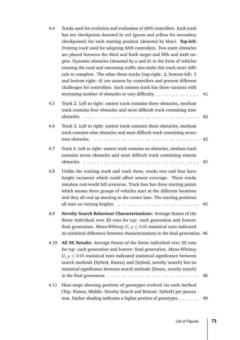
4.4 Tracks used for evolution and evaluation of ANN controllers. Each trackhas ten checkpoints denoted in red (green and yellow for secondarycheckpoints) for each starting position (denoted by blue). Top-left:Training track used for adapting ANN controllers. Two static obstaclesare placed between the third and forth target and fifth and sixth tar-gets. Dynamic obstacles (denoted by a and b) in the form of vehiclescrossing the road and oncoming traffic also make this track more diffi-cult to complete. The other three tracks (top-right: 2, bottom-left: 3and bottom-right: 4) are unseen by controllers and present differentchallenges for controllers. Each unseen track has three variants withincreasing number of obstacles to vary difficulty. . . . . . . . . . . . . . 41

4.5 Track 2. Left to right: easiest track contains three obstacles, mediumtrack contains four obstacles and most difficult track containing nineobstacles. . . . . . . . . . . . . . . . . . . . . . . . . . . . . . . . . . . 42

4.6 Track 3. Left to right: easiest track contains three obstacles, mediumtrack contains nine obstacles and most difficult track containing seven-teen obstacles. . . . . . . . . . . . . . . . . . . . . . . . . . . . . . . . 42

4.7 Track 4. Left to right: easiest track contains no obstacles, medium trackcontains seven obstacles and most difficult track containing sixteenobstacles. . . . . . . . . . . . . . . . . . . . . . . . . . . . . . . . . . . 43

4.8 Unlike the training track and track three, tracks two and four haveheight variances which could affect sensor coverage. These trackssimulate real-world hill scenarios. Track four has three starting pointswhich means three groups of vehicles start at the different locationsand they all end up meeting in the center lane. The starting positionsall start on varying heights. . . . . . . . . . . . . . . . . . . . . . . . . 43

4.9 Novelty Search Behaviour Characterisations: Average fitness of thefittest individual over 20 runs for top: each generation and bottom:final generation. Mann-Whitney U, p ≤ 0.05 statistical tests indicatedno statistical difference between characterisations in the final generation. 46

4.10 All NE Results: Average fitness of the fittest individual over 20 runsfor top: each generation and bottom: final generation. Mann-WhitneyU, p ≤ 0.05 statistical tests indicated statistical significance betweensearch methods [hybrid, fitness] and [hybrid, novelty search] but nostatistical significance between search methods [fitness, novelty search]in the final generation. . . . . . . . . . . . . . . . . . . . . . . . . . . . 48

4.11 Heat-maps showing portions of genotypes evolved via each method(Top: Fitness, Middle: Novelty Search and Bottom: Hybrid) per genera-tion. Darker shading indicates a higher portion of genotypes. . . . . . . 49

List of Figures 73

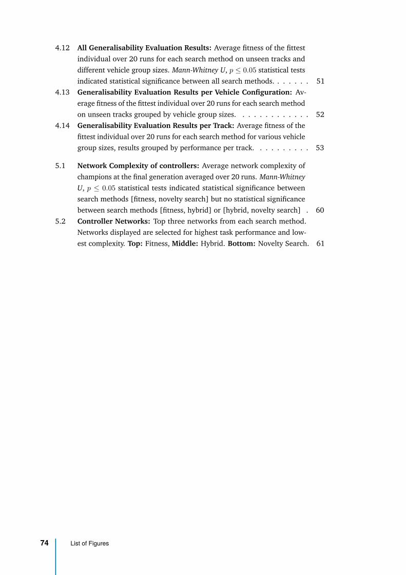
4.12 All Generalisability Evaluation Results: Average fitness of the fittestindividual over 20 runs for each search method on unseen tracks anddifferent vehicle group sizes. Mann-Whitney U, p ≤ 0.05 statistical testsindicated statistical significance between all search methods. . . . . . . 51

4.13 Generalisability Evaluation Results per Vehicle Configuration: Av-erage fitness of the fittest individual over 20 runs for each search methodon unseen tracks grouped by vehicle group sizes. . . . . . . . . . . . . 52

4.14 Generalisability Evaluation Results per Track: Average fitness of thefittest individual over 20 runs for each search method for various vehiclegroup sizes, results grouped by performance per track. . . . . . . . . . 53

5.1 Network Complexity of controllers: Average network complexity ofchampions at the final generation averaged over 20 runs. Mann-WhitneyU, p ≤ 0.05 statistical tests indicated statistical significance betweensearch methods [fitness, novelty search] but no statistical significancebetween search methods [fitness, hybrid] or [hybrid, novelty search] . 60

5.2 Controller Networks: Top three networks from each search method.Networks displayed are selected for highest task performance and low-est complexity. Top: Fitness, Middle: Hybrid. Bottom: Novelty Search. 61

74 List of Figures

List of Tables

4.1 Neuro-Evolution (NE) and Experiment Parameters. Parameters withminimal impact on evolution are excluded. . . . . . . . . . . . . . . . . . 40

4.2 Top: Experiment runtime parameters for NE controller adaptation.Bottom: Generalisability test runtime parameters. . . . . . . . . . . . 44

4.3 Schedule of Generalisability Experiments: Each of the listed experi-ments are run for all sixty controllers from the three evolutionary searchmethods. . . . . . . . . . . . . . . . . . . . . . . . . . . . . . . . . . . . 54

4.4 Mann-Whitney U Statistical Tests for each search method for con-troller evolution and generalisability evaluations. . . . . . . . . . . . . 55

4.5 Mann-Whitney U Statistical Tests for each search method per vehicleconfiguration, aggregated over tracks. . . . . . . . . . . . . . . . . . . 55

4.6 Mann-Whitney U Statistical Tests for each search method per track,aggregated over vehicle configurations. . . . . . . . . . . . . . . . . . . 56

75

Declaration

I know that plagiarism is wrong. Plagiarism is to use another’s work and pretendthat it is one’s own.

I have used the . . . . . . . . . . . . . . . . . . . . . . . . . . . . . . . . . convention for citation and refer-encing. Each contribution to, and quotation in this thesis, Neuro-Evolution SearchMethodologies for Collective Self-Driving Vehicles, from the work(s) of other peo-ple has been attributed, and has been cited and referenced.

This thesis, Neuro-Evolution Search Methodologies for Collective Self-Driving Ve-hicles, is my own work.

I have not allowed, and will not allow, anyone to copy my work with the intentionof passing it off as his or her own work.

Cape Town, October 2019


78 List of Tables

Date post:	16-Feb-2022
Category:	Documents
Upload:	others
View:	5 times
Download:	0 times