Neutral Property Taxation∗

Richard ArnottBoston College

September 1998

Abstract

This paper investigates property tax systems (linear taxes on pre-development land value, post-development structure value, and post-development site value) from a partial equilibrium perspective.Particular attention is paid to characterizing property tax systems that are neutral with respect to the timingand density of development and to calculating the deadweight loss from non-neutral property taxsystems.

JEL code: H2

Keywords: property taxation, site value taxation, land taxation, neutrality

Department of EconomicsBoston CollegeChestnut Hill, MA 02167USA

Tel: (617) 552-3674Fax: (617) 552-2308E-mail: richard.arnott@bc.edu

∗ I would like to thank seminar participants at the Universities of Alberta, British Columbia, Calgary,California-Berkeley, Cergy-Pontoise, Oldenberg and New Hampshire for helpful comments, andDennis Capozza, Yoshitsugu Kanemoto, Geoffrey Turnbull, and Helen Ladd for updating me on theliterature.

1

Neutral Property Taxation

Suppose, for the sake of argument, that a parcel of land has an “intrinsic value” that is unaffected

by decisions concerning its current use. A tax on such intrinsic value would be neutral — would not

affect decisions concerning its current or future use. This principle has led many economists through the

years to advocate the use of land value (or, synonymously, site value) taxation, and the replacement of

the current non-neutral property tax system with a land value tax system.

The obvious difficulty is to come up with a definition of land value that is not only neutral, but

also fair, practicable and sensible. If the market value of a plot of land depends only on the

“attractiveness” of its location (in contrast to the quality of servicing of the land, for example), a tax on

the market value of land is neutral. Even granting this condition, there is an unavoidable problem.

Because of the durability and immobility of structures, there is no “market” value for developed land.

The value observed in the market for a developed site is its property value. And there is no economically

correct way to decompose this value into land value and structure value.

During the 1970’s four papers (Shoup (1970), Skouras (1978), Bentick (1979), and Mills

(1981)) independently examined arguably the most intuitive decomposition, defining post-development

site value as property value minus the depreciated cost of the structure on the site. This definition, here

termed residual site value, is appealing because it is intuitive and would be relatively easy to implement

for tax purposes. The results of these papers can be obtained from a simple model of a developer who

owns a unit area of vacant land. He must decide, under perfect foresight, when to develop the property

and at what density. A land or property tax system is said to be neutral if its application does not alter the

developer’s timing or density decisions. What Shoup et al. (who collectively shall be referred to as the

revisionists) showed was that the taxation of residual site value is non-neutral; in particular, it

discourages density. This result received widespread attention since it called into question the

conventional wisdom concerning the neutrality of land taxation.

Subsequent work (Tideman (1982)) has shown that neutrality is achieved when post-

development site value is defined as “what the site would be worth if there were no structure on it” —

here termed raw site value — since this value is unaffected by the developer’s decisions. Use of this

2

hypothetical value has the disadvantage, however, that it cannot be simply calculated or inferred on the

basis of market observables. Thus, it would appear that the choice of definition of post-development site

value for site value taxation purposes entails a tradeoff between deviations for neutrality and

considerations of administrative feasibility.

This paper asks whether it is not possible to get the best of both worlds — to avoid the tradeoff

— with a well-chosen property tax system. More specifically, with separate tax rates on pre-

development land value, post-development residual site value, and structure value, is neutrality

achievable? Since there are three objectives — neutrality with respect to development timing, neutrality

with respect to development density, and expropriation of a desired fraction of value — and three

instruments, a positive answer is plausible. At least for the model employed — which assumes perfect

competition and no uncertainty, among other things — the paper proves that there is indeed a neutral

property tax system which employs the residual definition of site value. This positive result provides a

basis for optimism in the search for a property tax system that is both practicable and close to neutral.

The paper goes on to derive the tax rates that achieve neutrality for the special case where post-

development rents grow at a constant rate and vacant land generates no rent: Pre-development land value

is untaxed, post-development residual site value is taxed at a rate chosen to meet the revenue requirement,

and structure value is subsidized. The paper also provides the first — to my knowledge — derivation of

the deadweight loss from non-neutral site and property value taxation.

Section I sets the stage by providing a detailed synthetic review of the literature. Section II

presents the analytical results concerning neutral property taxation, and briefly discusses some of the

problems that would be encountered in moving from theory to practice. Section III derives the

deadweight loss from non-neutral property tax systems. Section IV summarizes and concludes.

I. Setting the Stage

To begin, a few words on terminology are appropriate. First, throughout the paper, the terms

land value and site value are employed completely interchangeably. Second, a distinction is made

between a land value tax system and a property tax system. A land or site value tax system taxes only

3

land or site value and at the same rate before and after development. According to the usage in the paper,

the basis for land taxation prior to development is simply the market value of the vacant land. After

development, however, when there is a durable and immobile structure on the site, there are not separate

market values for the site and the structure. Site value is then an abstract or hypothetical notion; it must

be imputed. As we shall see, whether site value taxation is neutral hinges on the definition of post-

development site value employed. A property tax system, meanwhile, is characterized by three tax rates:

a tax rate on the market value of vacant land which applies prior to development, and separate post-

development tax rates on site value and structure value. Thus, according to this terminology, a land

value tax system is a special case of a property tax system.

Under a site or land value tax system, the same tax rate is applied to land value before and after

development. This need not be the case under a property tax system. Accordingly, the site value tax rate

under a land value tax system is the tax rate applied to both pre-development land value (a market value)

and post-development land value (a hypothetical value). When discussing property tax systems, a

distinction must be made between the tax rate on pre-development and post-development land value. The

former is referred as the tax rate on vacant land and the latter as the site value tax rate.

I.1 Synthesis of the Literature on the Taxation of Land

The previous literature has employed a variety of models. All the qualitative results obtained can,

however, be illustrated using variants of the Arnott-Lewis (1979) model of the transition of land to urban

use. An atomistic landowner owns a unit area of undeveloped land. He must decide when to develop

the land and at what density to build the structure. Once built, the structure is immutable; no depreciation

occurs and no redevelopment is possible. He makes his decision under perfect foresight (and hence

under no uncertainty).

To start, consider the landowner-developer’s problem in the absence of taxation. The following

notation is employed:

t time (t=0 today)

T development time

K development density (the capital-land ratio)

4

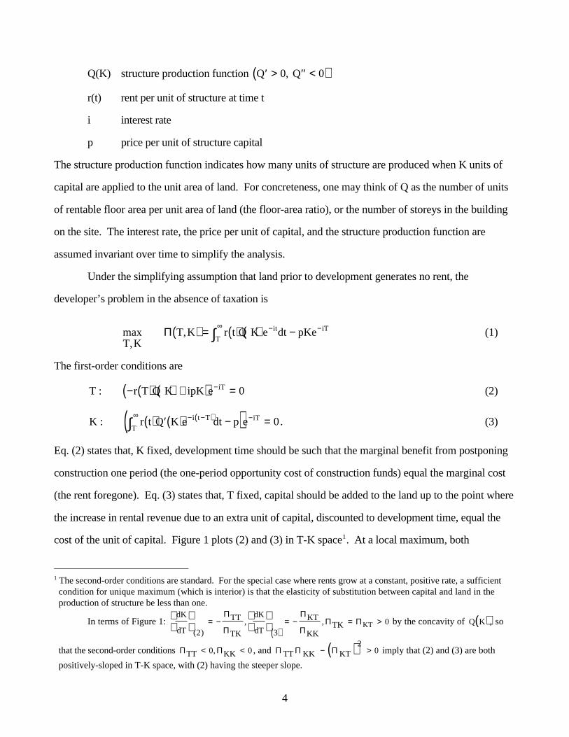
Q(K) structure production function ′ > ′′ <( )Q Q0 0,

r(t) rent per unit of structure at time t

i interest rate

p price per unit of structure capital

The structure production function indicates how many units of structure are produced when K units of

capital are applied to the unit area of land. For concreteness, one may think of Q as the number of units

of rentable floor area per unit area of land (the floor-area ratio), or the number of storeys in the building

on the site. The interest rate, the price per unit of capital, and the structure production function are

assumed invariant over time to simplify the analysis.

Under the simplifying assumption that land prior to development generates no rent, the

developer’s problem in the absence of taxation is

max,

,T K

T K r t Q K e dt pKeT

it iTΠ( ) = ( ) ( ) −∞ − −∫ (1)

The first-order conditions are

T r T Q K ipK e iT: − ( ) ( ) +( ) =− 0 (2)

K r t Q K e dt p eT

i t T iT: ( ) ′( ) −( ) =∞ − −( ) −∫ 0 . (3)

Eq. (2) states that, K fixed, development time should be such that the marginal benefit from postponing

construction one period (the one-period opportunity cost of construction funds) equal the marginal cost

(the rent foregone). Eq. (3) states that, T fixed, capital should be added to the land up to the point where

the increase in rental revenue due to an extra unit of capital, discounted to development time, equal the

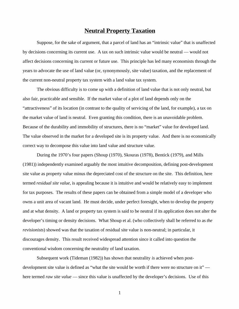
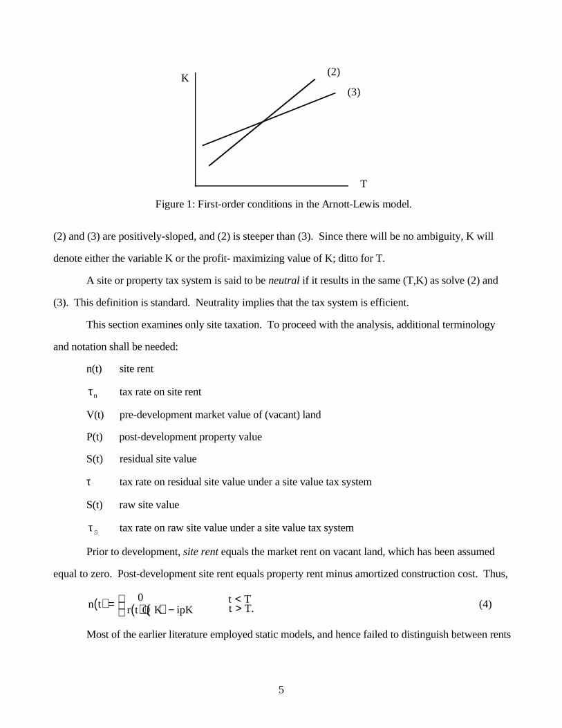
cost of the unit of capital. Figure 1 plots (2) and (3) in T-K space1. At a local maximum, both

1 The second-order conditions are standard. For the special case where rents grow at a constant, positive rate, a sufficientcondition for unique maximum (which is interior) is that the elasticity of substitution between capital and land in theproduction of structure be less than one.

In terms of Figure 1: dK

dT

TT

TK

dK

dT

KT

KKTK KT

= − = − = >

( )( ), ,

2 30

Π

Π

Π

ΠΠ Π by the concavity of Q K( ), so

that the second-order conditions Π ΠTT KK< <0 0, , and Π Π ΠTT KK KT− >( )20 imply that (2) and (3) are both

positively-sloped in T-K space, with (2) having the steeper slope.

5

K

T

(2)

(3)

Figure 1: First-order conditions in the Arnott-Lewis model.

(2) and (3) are positively-sloped, and (2) is steeper than (3). Since there will be no ambiguity, K will

denote either the variable K or the profit- maximizing value of K; ditto for T.

A site or property tax system is said to be neutral if it results in the same (T,K) as solve (2) and

(3). This definition is standard. Neutrality implies that the tax system is efficient.

This section examines only site taxation. To proceed with the analysis, additional terminology

and notation shall be needed:

n(t) site rent

τn tax rate on site rent

V(t) pre-development market value of (vacant) land

P(t) post-development property value

S(t) residual site value

τ tax rate on residual site value under a site value tax system

S(t) raw site value

τS tax rate on raw site value under a site value tax system

Prior to development, site rent equals the market rent on vacant land, which has been assumed

equal to zero. Post-development site rent equals property rent minus amortized construction cost. Thus,

n t r t Q K ipKt Tt T( ) = ( ) ( ) −

<>

0 . (4)

Most of the earlier literature employed static models, and hence failed to distinguish between rents

6

and values. The first economists to use dynamic models, the revisionists, employed the residual site

value definition of site value. Pre-development residual site value is the pre-development market value of

land. Post-development residual site value equals property value minus depreciated structure value.

Here the depreciation rate is assumed to be zero. Accordingly,

S tV t

P t pKt Tt T( ) = ( )

( ) −

<> . (5)

As we shall see, with the residual definition of site value, site value taxation is distortionary. It

has subsequently been recognized (e.g., Tideman (1982), Netzer (1997), and Ladd (1997) whom will be

referred to collectively as defenders of the orthodoxy) that the neutrality of site value taxation can be

recovered by employing definitions of site value that have the feature that post-development site value is

unaffected by the timing and density of development chosen by the market. One such definition of site

value is raw site value. Pre-development raw site value — like pre-development residual site value — is

the market value of vacant land. Post-development raw site value is what the site would sell for were

there no structure on it (even though there in fact is). Thus,

S t

V tt

t Tt T( ) = ( )

( )

<>Φ , (6)

where Φ t( ) is “what the site would sell for were there no structure on it”, an expression for which shall

be derived subsequently.

The literature contains five principal results relating to land/site taxation. The following review

states each result, proves it, and provides the economic intuition.

• Result 1 : A “pure” land value tax — one which is imposed on the “intrinsic” value of the land,

independent of the developer’s decision concerning the timing and density of development — is neutral.

Proof : Since the tax payable is independent of the developer’s decisions, he views such a tax as a

lump sum tax, so it does not affect his decisions. þ

This is the idea underlying the neutrality of land value taxation. The neutrality result holds

however the intrinsic value of the land is calculated (as long as it is independent of the developer’s

decisions) and whether the tax rate is constant or variable over time.

7

• Result 2 : A linear, time-invariant tax on site rent is neutral.

Proof : The developer chooses T and K to maximize the discounted present value of rent, less

construction costs, less tax payments:

max,T K

r t Q K e dt pKe n t e dtT

it iTnT

it( ) ( ) − − ( )∞ − − ∞ −∫ ∫ τ

= ( ) ( ) − − ( ) ( ) −( )∞ − ∞ − ∞ −∫ ∫ ∫r t Q K e dt ipKe dt r t Q K ipK e dtT

it

T

itnT

itτ (using (4))

= −( ) ( ) ( ) −( )∞ −∫l r t Q K ipK e dtn T

itτ . (7)

The maximizing choices of T and K are independent of τn . þ

In the absence of taxation, the developer chooses T and K to maximize the

discounted present value of site rent. With site rent taxation at rate τn , the developer chooses T and K to

maximize the discounted present value of site rent net of the tax payment. Since the tax equals τn times

site rent, the maximizing T and K are unaffected by the tax. Site rent is analogous to profit, and the

neutrality of site rent taxation analogous to the well-known neutrality of a time-invariant tax on pure

profit.

Observe that, with durable structures, a site rent tax whose tax rate is time-varying is not in

general neutral. Such a tax does not affect the timing first-order condition, but it does distort the density

first-order condition. To see this, consider the top storey of a building in the no-tax situation. Suppose

in the early years of the building’s life, from T to t , that the top storey loses money (its net rent is

negative: r t Q K ip( ) ′( ) − < 0), with these losses being exactly offset in discounted terms by profits in

later years. Now impose a site rent tax that is set at a positive rate from T to t and at a zero rate

thereafter. The top storey is subsidized from T to t and incurs no tax liability thereafter. This particular

time-varying site rent tax would encourage construction at higher density than in the no-tax situation.

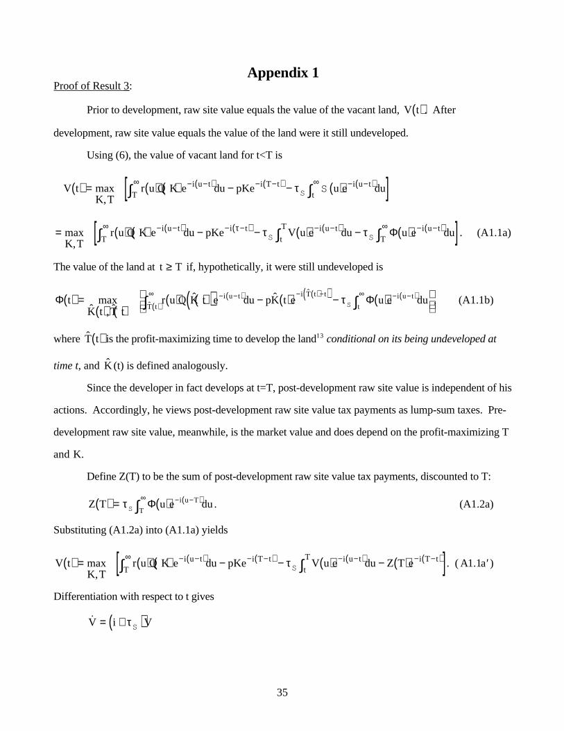
• Result 3 : A linear, time-invariant tax on raw site value is neutral.

Proof : See Appendix 1.

The intuition for this result was given earlier.

8

• Result 4 : If structures are perfectly malleable or mobile — so that the developer chooses the function

K(t) — site value taxes are neutral.

Proof : To simplify, assume that ′( ) = ∞Q 0 , so that development occurs at all points in time.

Since capital may be regarded as being mobile — rented at ip per unit per unit time — the market value

of land is well-defined. Consequently, there is no ambiguity in the definition of site value, which we

denote by Σ t( ):

Σ ΣΣtK u

r u Q K u e du ipK u e du u u e dut

i u t

t

i u t

t

i u t( ) =( )

( ) ( )( ) − ( ) − ( ) ( )∞ − −( ) ∞ − −( ) ∞ − −( )∫ ∫ ∫max τ , (8)

when τΣ u( ) is the site value tax rate at time u. Since structures are perfectly malleable, there is no

development timing condition. Differentiating (8) w.r.t. t yields

Σ Σ ΣΣt r t Q K t ipK t i t t t( ) = − ( ) ( )( ) + ( ) + ( ) + ( ) ( )τ ,

and solving gives

Σ ΣtK u

r u Q K u ipK u e dui u du

ttu

( ) =( )

( ) ( )( ) − ( )( ) − + ′( )( ) ′∫∞∫max τ , (9)

from which it is evident that site value taxation does not affect development density. þ

The intuition is straightforward. Today’s site value is essentially independent of today’s capital

intensity, and future site values completely independent of it. Thus, in deciding on today’s capital

intensity, the developer views the present value of future site value tax liabilities as a lump sum, and

hence his capital intensity decision is unaffected by site value taxation.2

Return to the situation where the development decision is completely irreversible — once

vacant land is developed at a certain density, it remains at that density forever.

• Result 5 : A linear, time-invariant tax on residual site value is distortionary

Proof :

2 It is straightforward to demonstrate that with perfect malleable structures site rent taxation is neutral with a time-varyingtax rate.

9

S t K Tr u Q K e du pKe S u e dt t T

r u Q K e du pK S u e dt t T

T

i u t i T t

t

i u t

t

i u t

t

i u t

( ) =( ) ( ) − − ( ) <

( ) ( ) − − ( ) >

∞ − −( ) − −( ) ∞ − −( )

∞ − −( ) ∞ − −( )

∫ ∫

∫ ∫

max,

.

τ

τ(10)

Solving S(t) by the now-familiar procedure yields

S t K Tn u e du t T

n u e du t T

T

i u t

t

i u t

( ) =( ) <

( ) >

∞ − +( ) −( )

∞ − +( ) −( )

∫

∫

max,

.

τ

τ(11)

The first-order condition with respect to development time is unaffected by the site value tax: n T( ) = 0 .

The first-order condition with respect to density is, however, distorted. In particular, the tax on residual

site value has the effect of increasing the discount rate on site rent from i to i + τ . þ

The marginal cost of postponing development equals the rent forgone, and the marginal benefit

from postponing development equals the interest on construction costs plus net tax savings. Since

residual site value is the same immediately before and immediately after development and since the tax

rate on pre-development site value is the same as that on post-development site value, the net tax savings

from postponing development equal zero, and the timing first-order condition reduces to what it is in the

absence of the residual site value tax.

Two different intuitions for why the residual site value tax distorts the development density first-

order conditions are now presented. To simplify, consider the normal case in which rents rise

monotonically over time. The developer will add storeys to his building up to the point where the

discounted net rent from the top storey equals zero, with the negative net rent in earlier years of the

building’s life just being offset, in discounted terms, by the positive net rent achieved in later years. The

residual site value tax raises the discount rate, which puts greater weight on the earlier years when net

rent is negative. Thus, the top storey that just broke even in the absence of the tax loses money when the

tax is imposed (holding development time constant), implying that the rise in the discount rate caused by

the residual site value tax lowers profit-maximizing development density (holding development time

constant). An alternative explanation is as follows. Start with the situation without the residual site value

tax. At development time, the top storey of the building just breaks even. In other words, at

10

development time the increment to residual site value from the top storey is zero. Subsequent to

development time, the present value of rent from the top storey increases while the present value of

amortized construction costs remains constant. Thus, after development time the increment to residual

site value from the top storey is positive (and increasing over time). When, therefore, a residual site

value tax is imposed, the top storey adds to the building’s discounted tax liability. Imposition of the

residual site value tax therefore renders the top storey of the building unprofitable. The residual site

value tax therefore discourages density.

The essential difference between raw site value and residual site value taxation should now be

apparent. Post-development raw site value is unaffected by the density of development, while in the

neighborhood of the optimum post-development residual site value is increasing in the density of

development. Thus, imposition of a raw site value tax has no effect on the development density

condition, while imposition of a residual site value tax discourages density.

To recapituate: Result 4 was that with perfectly mobile and malleable structure capital, site value

taxation is neutral. Results 2, 3, and 5 were derived for the opposite extreme where structure capital is

completely immobile and immalleable, but apply as well for intermediate situations where capital can be

moved but at a cost and where density can be altered but with adjustment costs. Result 2 was that a

linear tax on site rent, at a time-invariant rate, is neutral; result 3 was that a linear tax on raw site value, at

a time-invariant rate, is neutral; and result 5 was that a linear tax on residual site value is non-neutral.

Thus, the non-neutrality of residual site value taxation derives from a combination of the immobility and

immalleability of structure capital, the taxation of site value rather than site rent, and the particular

definition of site value employed.

I.2 Practicability of Alternative Definitions of Site Value

The economists who have written recently on site value taxation can be divided into two camps.

Defenders of the orthodoxy and modern Georgists3 view it almost as an article of faith that site value

3 Henry George was an influential, late-eighteenth century Progressive American reformer who argued in favor of a singletax — a confiscatory tax on land values. Modern Georgists, while not generally adhering to George’s view that aconfiscatory tax on land values is the single tax needed for optimal taxation, subscribe to the view that land value taxationis efficient.

11

taxation is neutral. They have therefore objected strongly to assertions that site value taxation is

distortionary (Tideman (1982), Netzer (1997)). Their view is not unreasonable. Results 1 and 3 of the

previous subsection show that land or site value can be defined so that site value taxation is non-

distortionary; raw site value is one such definition. The revisionists, however, employ an alternative

definition of site value, residual site value. As with raw site value, pre-development residual site value

equals the market value of land. In contrast to the definition of raw site value, however, post-

development residual site value is measured by property value minus structure value. Under this

definition, site value taxation is indeed distortionary, as was shown in Result 5.

The difference between the two camps therefore derives from differences in the definition of post-

development site value, which reflects the absence of separate market values for land and structure on a

developed site. The choice of the definition of post-development site value should be made on pragmatic

grounds. Employing the raw site value definition has the advantage that its use results in a site value tax

that is neutral. The residual site value definition has the advantage that its computation, though not

without contentious aspects, is relatively straightforward.

Vickrey (1970) characteristically understood the economics of site value taxation before anyone

else and also characteristically leaned as far as could reasonably be defended towards the theoretically

nice policy: “On the whole --- I am inclined to recommend sticking as closely as possible to a

theoretically defined [land or site] value” (p.36). But he also acknowledged that “ In the end it seems

likely that some degree of departure from the goal of strict neutrality will have to be accepted in order to

achieve an acceptable degree of administrative feasibility” (p. 29).

I place more weight on administrative feasibility. The further one moves away from a definition

of site value based on market observables, the more capricious4, unfair, and prone to corruption is site

value taxation in practice likely to be. Furthermore, the more capricious the tax system, the greater the

amount of wasteful litigation. To reduce appeals, assessments for property tax purposes are now

routinely based on hedonic price analysis. A site value tax system that defined site value in a way that

4 One can imagine a clerk in the Assessment Department of Sticks, Anystate, confronted with the task of computing rawpost-development site value!

12

could not be strongly defended in court, on the basis of market observables, would invite appeals, and

for that reason would come to be replaced by a system that defined site value on the basis of market

observables. Defining site value as residual site value is not ideal in this regard, since imputed post-

development structure value is measured by the depreciated construction costs, which are not simple to

estimate. Style obsolescence is hard to measure, and depreciation due to quality deterioration is not only

hard to measure but also depends on the level of maintenance chosen which reflects market conditions

(Sweeney (1974)). Nevertheless, studies have been undertaken which estimate average rates of

depreciation on structures, as captured by age-of-building variables (e.g., Chinloy (1979)), and the

results of such studies could be employed to impute post-development structure value. Thus, with

hedonic price analysis being employed to estimate post-development property value, residual site value

could be imputed using methods that are both straightforward and ‘scientific’, and therefore readily

defensible in court. Hence, on grounds of both administrative costs and fairness, I favor defining site

value as residual site value.

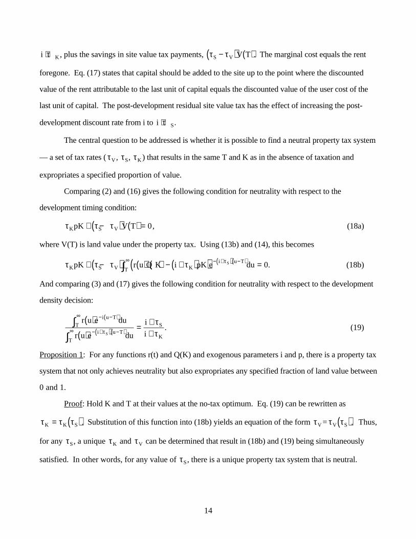
Residual site value taxation is, however, distortionary; in particular, it discourages density. A

question then arises which, surprisingly, has not been addressed in the literature: Is it possible to design

a property tax system — defined as linear taxes at different rates that are constant over time on pre-

development land value, post-development site value, and post-development structure value — that

employs the residual definition of site value and which is neutral or close to neutral? The next section

takes up this question.

II. Neutral or Near-neutral Property Taxation

II.1 Analysis and Results

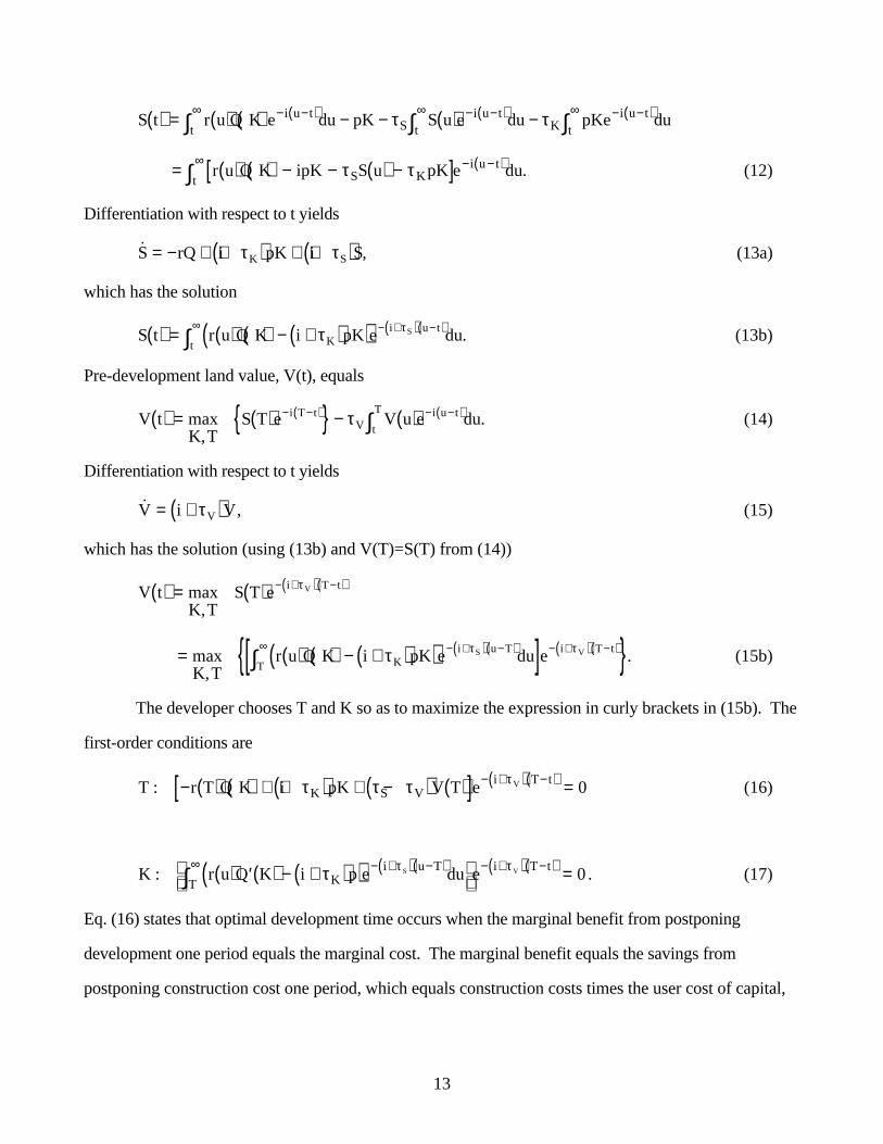
The valuation formulae are now derived for the model of the previous section, but with a property

tax system instead of a site value tax system. The property tax system is characterized by a linear tax on

pre-development land value at rate τV , a linear tax on post-development residual site value at rate τS , and

a linear tax on post-development structure value at rate τK .

Post-development residual site value is

13

S t r u Q K e du pK S u e du pKe dut

i u tS t

i u tK

i u tt

( ) = ( ) ( ) − − ( ) −∞ − −( ) ∞ − −( ) − −( )∞∫ ∫ ∫τ τ

= ( ) ( ) − − ( ) −[ ]∞ − −( )∫ r u Q K ipK S u pK e duS Kti u tτ τ . (12)

Differentiation with respect to t yields

S rQ i pK i SK S= − + +( ) + +( )τ τ , (13a)

which has the solution

S t r u Q K i pK e duKt

i u tS( ) = ( ) ( ) − +( )( )∞ − +( ) −( )∫ τ τ . (13b)

Pre-development land value, V(t), equals

V tK T

S T e V u e dui T tV t

T i u t( ) = ( ){ } − ( )− −( ) − −( )∫max,

.τ (14)

Differentiation with respect to t yields

V i VV= +( )τ , (15)

which has the solution (using (13b) and V(T)=S(T) from (14))

V tK T

S T e i T tV( ) = ( ) − +( ) −( )max,

τ

= ( ) ( ) − +( )( )[ ]{ }− +( ) −( )∞ − +( ) −( )∫max,

.K T

r u Q K i pK e du eKi u T

T

i T tS Vτ τ τ (15b)

The developer chooses T and K so as to maximize the expression in curly brackets in (15b). The

first-order conditions are

T r T Q K i pK V T eK S Vi T tV: − ( ) ( ) + +( ) + −( ) ( )[ ] =− +( ) −( )τ τ τ τ 0 (16)

K r u Q K i p e du eKT

i u T i T tS V: ( ) ′( ) − +( )( )

=∞ − +( ) −( ) − +( ) −( )∫ τ τ τ 0 . (17)

Eq. (16) states that optimal development time occurs when the marginal benefit from postponing

development one period equals the marginal cost. The marginal benefit equals the savings from

postponing construction cost one period, which equals construction costs times the user cost of capital,

14

i K+ τ , plus the savings in site value tax payments, τ τS V V T−( ) ( ). The marginal cost equals the rent

foregone. Eq. (17) states that capital should be added to the site up to the point where the discounted

value of the rent attributable to the last unit of capital equals the discounted value of the user cost of the

last unit of capital. The post-development residual site value tax has the effect of increasing the post-

development discount rate from i to i S+ τ .

The central question to be addressed is whether it is possible to find a neutral property tax system

— a set of tax rates ( τ τ τV S K, , ) that results in the same T and K as in the absence of taxation and

expropriates a specified proportion of value.

Comparing (2) and (16) gives the following condition for neutrality with respect to the

development timing condition:

τ τ τK S VpK V T+ −( ) ( ) = 0 , (18a)

where V(T) is land value under the property tax. Using (13b) and (14), this becomes

τ τ τ τ τK S V KT

i u TpK r u Q K i pK e duS+ −( ) ( ) ( ) − +( )( ) =∞ − +( ) −( )∫ 0. (18b)

And comparing (3) and (17) gives the following condition for neutrality with respect to the development

density decision:

r u e du

r u e du

i

i

i u T

Ti u T

T

S

KS

( )( )

= ++

− −( )∞

− +( ) −( )∞∫

∫ τ

ττ

. (19)

Proposition 1 : For any functions r(t) and Q(K) and exogenous parameters i and p, there is a property tax

system that not only achieves neutrality but also expropriates any specified fraction of land value between

0 and 1.

Proof : Hold K and T at their values at the no-tax optimum. Eq. (19) can be rewritten as

τ τ τK K S= ( ) . Substitution of this function into (18b) yields an equation of the form τV = τ τV S( ). Thus,

for any τS , a unique τK and τV can be determined that result in (18b) and (19) being simultaneously

satisfied. In other words, for any value of τS , there is a unique property tax system that is neutral.

15

From (13b), setting τS = ∞ expropriates all of the no-tax site value while setting τS = 0

expropriates none of the no-tax site value (since with τS = 0 , τK and τV are also zero). From (19),

τ τK S( ) is a continuous function of τS . From (13b), S(T) is therefore a continuous function of τS .

Thus, there is a τS ∈ ∞[ )0, such that any specified proportion of site value between 0 and 1 is

expropriated.5 þ

The general relationship between τ τ τV S K, , and in a neutral tax system is complex and is

investigated in Appendix 2. A complete characterization of the relationship between τ τ τV S K, , and for

the special case where rents grow exponentially over time can, however, easily be obtained. The growth

rate of rents is denoted by η >( )0 . 6

Proposition 2 : When rents grow at a constant rate η, a neutral property tax system has the properties

that:

i) τ τ ητ ηK S

Si= −

+ −

ii) τV = 0

Proof : i) follows directly from (19). ii) then follows from (18b), after substitution of i). þ

We provide two different intuitive explanations for the results in Proposition 2. The first is

casual, the second exact. The residual site value tax system considered in the previous section is a

special case of the class of property tax systems considered here, with τ τ τ= =V S and τK = 0 . Recall

(proof of Result 5) that that tax system had no effect on the development timing condition but caused the

development density condition to change in such a way that discourages density. Take the residual site

value tax system as the starting point and consider how τ τ τS V K, , and should be modified to restore

neutrality. First, capital should be subsidized to offset the depressing effect of residual site value taxation

on development density. But from (16a), the subsidization of capital reduces the marginal benefit from

postponing development. The development timing condition, which was undistorted with residual site

5 Observe that the proof generalizes to the situation where i, p, and Q(K) are all functions of time.

16

value taxation, becomes distorted, leading to excessively early development. This can be corrected by

setting the pre-development land value tax rate below the post-development site value tax rate. This

intuition suggests that, a neutral property tax system which raises positive revenue has τ τS V> and

τK < 0 . This intuition is consistent with Proposition 2 which concerns a special case, but is not correct

in general (see Appendix 2).

The precise intuition is based on a result that is sufficiently important that we present it as:

Proposition 3 : When rents grow at the constant rate η, the neutral property tax system described in

Proposition 2 is equivalent to a site rent tax system with the constant tax rate τ ττ ηn

S

Si=

+ −.

Proof : Since both tax systems are neutral and hence have the same development time and

density, it suffices to demonstrate that the time paths of tax revenue collected under the two tax systems

coincide. For both, the tax revenue collected prior to development is zero. After development, the time

path of revenue collected under the site rent tax is

R t r t Q K ipKn( ) = ( ) ( ) −( )τ . (20)

With a property tax system, the time path of revenue collected is

R t S t pKS K( ) = ( ) +τ τ

= ( ) ( )+ −

−+( )+

+ττ η

τ ττ

τSS

S K

SK

r t Q K

i

i pK

ipK (using (13b)). (21)

Now substitute property i) of the neutral property tax system into (21):

R ti

r t Q K ipKS

S

( ) =+ −

( ) ( ) −( )ττ η

. (22)

With τ ττ ηn

S

Si=

+ −, the two tax revenue streams are identical. þ

Proposition 3 has an immediate:

Corollary : With rents growing at a constant rate η: i) at every point in time, the ratio of property tax

revenue collected under a neutral property tax system to site rent equals τ τ ηS Si + −( ) ; and

6 A necessary condition for a local maximum is that rents be growing at development time.

17

ii) the ratio of the present value of property tax revenue collected under a neutral property tax system to

the no-tax pre-development land value (for t T< ) or no-tax post-development residual site value (for

t T> ) — which is one measure of the proportion of value expropriated by the tax system — equals

τ τ ηS Si + −( ) .

Part i) of the Corollary follows immediately from the proof to Proposition 3. Part ii) follows

from part i). The Corollary is related to the second part of Proposition 1. There it was shown that there

exists a neutral property tax system that expropriates any desired proportion of the no-tax site value.

Proposition 3 gives the exact relation between τS and the proportion of no-tax site value expropriated,

for the special case of a constant growth rate of rents.

Another useful result for the situation where rents grow at a constant rate is given in:

Proposition 4 : Under the neutral property tax system described in Proposition 2, property value at

development time, site value at development time, and structure value are in the proportions: τ τS K− ,

−τK , τS .

The rest of this section discusses the implications of the above results for the design of a

practicable and neutral or close-to-neutral property tax system.

II. 2 Discussion

Since site rent taxation at a time-invariant rate is neutral, why not employ such a site rent tax

rather than a more complex neutral property tax system? The primary reason is presumably that site rents

are generally unobservable and would be difficult to estimate. While the estimation of pre-development

land value, post-development property value, and structure value is by no means trivial, there is a wealth

of practical experience to draw on. This observation points to the importance of considering the

informational feasibility of implementing alternative property tax systems.

Is implementation of the neutral property tax system derived in the previous subsection

informationally feasible? At first glance, the answer would appear negative since the optimal tax rates on

a parcel depend on that parcel’s future time path of rents, which is of course unknown. While the market

does not directly signal expectations concerning future rents, it does provide some information relevant to

18

computing the optimal tax rates: prior to development, the market value of the parcel, and immediately

after development, development time, development density, and property value. The question is whether

this information is sufficient to calculate the set of tax rates that achieves neutrality and raises the desired

revenue or expropriates the desired proportion of value. An incomplete answer, in terms of the model

(which entails the assumptions, inter alia, that the rent on vacant land is zero and that the interest rate is

time-invariant,) is that this information is sufficient if post-development rents grow at a constant rate, but

not generally otherwise. Under these circumstances, Proposition 2 indicates that τV = 0 , Proposition 4

that τ τK S S T pK= − ( )( ), and A2 9. ′′( ) in Appendix 2 that τ ε εS i pK pK S T= −( ) + ( )( )1 , where ε is

the desired proportion of value to expropriate. This assumes that developers take tax rates as parametric.

If, however, the government were to compute τK for a particular property from τ τK S S T pK= − ( )( ) on

the basis of that property’s S T pK( ) , the developer would take into account that by altering the density

of development he would alter the subsidy rate on capital, which would lead to non-neutrality.7 This

problem is easily overcome by setting a particular property’s τK on the basis of the S T pK( ) ratio for

“comparable”, recently developed properties.

When, however, rents do not grow at a constant rate, the situation is more complicated.

Neutrality in general requires a non-zero tax rate on (pre-development) land value. But prior to

development, the only information the market provides relevant to the future rental stream is land value.

7 Substitution of τ τK S S T pK= − ( )( ) into (13b) gives

= ( ) ( ) − + ( )( ) − +( ) −( )∞∫ r u Q K ipK S T e duS

i u T

TSτ τ

⇒ ( ) = + ( ) ( ) −( ) − +( ) −( )∞∫S T

i

ir u Q K ipK e duS i u T

TS

τ τ. (i)

Thus

V tK T

i

ir u Q K ipK e du eS i u T

T

i T tS V( ) = + ( ) ( ) −( )

− +( ) −( )∞ − +( ) −( )∫max,

τ τ τ , (ii)

which yields the following first-order conditions for T and K:

Ti

ie r T Q K ipK V TS i T t

S VV:

+ − ( ) ( ) + + −( ) ( )[ ] =− +( ) −( )τ τ ττ 0 (iii)

Ki

ie r u Q K ip e duS i T t i u T

TV S: .

+ ( ) ′( ) −( )[ ] =− +( ) −( ) − +( ) −( )∞∫

τ τ τ 0 (iv)

Timing neutrality requires τ τS V= . But with τ τS V= > 0 the density decision is distorted — density is discouraged.

19

This and the time at which the land value tax is first imposed do not provide enough information to

compute τV .

Intuition suggests that practically the market is sufficiently uncertain concerning the time path of

future rents that it has only weak beliefs concerning how the time path of future rents will differ from a

constant-growth-rate time path. This suggests that employing a property tax that would be neutral if the

future growth rate of rents were constant would normally come close to achieving neutrality.

Examination of this conjecture will require extending the model to allow for uncertainty (which could

build on Capozza and Li ( )).

The above argument suggests that design of a near-neutral property tax system is informationally

feasible. What of administrative feasibility? The analysis of the previous subsection applied to an

isolated property. If the tax system were to be applied as modeled, every property would have its own

post-development site value tax rate and structure value subsidy rate, which would be very cumbersome.

And since all tax rates on developed properties would have been set in the past, the government would

have no discretion to raise or lower tax revenues in the short run. Clearly, administrative feasibility

requires adapting the property tax system analyzed in the previous subsection.

The objective therefore is to find a property tax system that is informationally and administratively

feasible and that comes close to being neutral. It was argued earlier that a residual site value tax system is

both informationally and administratively feasible. Its weakness is that it discourages density. These

observations suggest the following simple adaptation of the neutral property tax system analyzed earlier.

After development, impose a residual site value tax along with a structure investment tax credit. The tax

rate on pre-development land value would be zero; the tax rate on post-development site value would be

set annually according to the government’s revenue requirements, etc.; and the tax credit rate on structure

investment would be set annually with the objective of achieving neutrality with respect to the timing and

density of development.

Implementation of such a tax system would require addressing a number of practical issues:

How finely should the tax credit rate on structure investment be varied over space? How should the

20

transition from the current system to this system be designed so as to achieve a smooth revenue stream,

to avoid causing a building boom or bust, and to be politically acceptable, which requires among other

things not generating substantial capital losses on any major class of properties? And how should the tax

credit rate on structure investment be determined? This tax system is only one of many that might attain

the best balance between practicability and deviation from neutrality, and has been presented more as a

basis for discussion than as a proposal.

The derivation of neutral property tax systems presented in the previous subsection made a large

number of simplifying assumptions. Future research should investigate how the results need to be

modified when account is taken of time variation in the interest rate and the price of structure capital,

technological change in construction, maintenance and depreciation, the possibility of redevelopment,

and uncertainty, and when time variation of the tax rates is considered.

III. The Deadweight Loss from Non-Neutral Property and Site Value Taxation 8

Remarkably, it appears that no one has investigated the deadweight loss associated with

alternative property tax systems from the modern perspective which correctly views the tax as a tax on

value (rather than rent) in a dynamic economy. The aim of the section is to present some preliminary

results rather than an exhaustive analysis.

III.1 τV > 0 from time immemorial

The first case considered is that where a positive tax on land value has been applied from t = −∞ .

To simplify the algebra slightly, values are evaluated at t=0. Where R(t) is the value of tax revenue

discounted or brought forward to time t,

R 0( ) = ( ) + + ( )−∞

− −∞ ∞ −∫ ∫ ∫τ τ τVT it

Kit

T S T

itV t e dt pKe dt S t e dt . (25)

Also,

S T r t Q K e dt pK pKe dt S t e dti t T

T Ki t T

T S T

i t T( ) = ( ) ( ) − − − ( )− −( )∞ − −( )∞ ∞ − −( )∫ ∫ ∫τ τ . (26)

Substituting (26) into (25), and simplifying, yields

21

R 0( ) = ( ) − − ( ) + ( ) ( )−∞

− − − ∞ −∫ ∫τVT it iT iT

T

itV t e dt pKe S T e r t Q K e dt . (27)

Finally, substituting

V t e i T tV( ) ( ) − +( ) −( )= V T τ (28)

into (27), and using S T V T( ) = ( ) , gives

R 0( ) = ( ) ( ) −∞ − −∫ r t Q K e dt pKeT

it iT . (29)

To evaluate the deadweight loss from the tax system, additional notation shall be employed. Let

bdenote the pre-tax situation, a the after-situation, L t( ) the landowner’s surplus evaluated at t, and

D t( ) deadweight loss at t.

The landowner’s surplus evaluated at t=0 is

Lb iT b

V T e0( ) = ( )( )− (30a)

La

Vi T tT iT

a

V T V t e dt e0 0( ) = ( ) − ( )( )

=−( )−∞

−∫τ (using (27) and (29)). (30b)

Thus, whatever the tax rate, as long as τV > 0 , the landowner’s surplus is driven to zero by the tax

system.

Since, in the partial equilibrium model employed in the paper, the structure rent stream and hence

the utility of renters is unaffected by taxation, the loss in social surplus is simply the sum of the loss in

landowner and government surplus. Thus,

D = L R L0 0 0 0( ) ( ) − ( ) + ( )( )b a

= ( )( ) − ( )V T eiT bR 0 . (31)

Defining

Y r t Q K e dt pKeb it

T

iTb

≡ ( ) ( ) −( )−∞ −∫

and Ya accordingly,

8 I would like to thank seminar participants in the Urban Land Division, Faculty of Commerce, University of BritishColumbia, for suggesting I treat the topic of this section.

22

D 0( ) = −Y Yb a . (32)

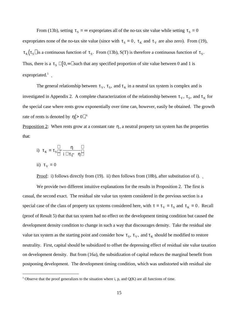
Note from (29) and (30b) that whatever the tax rate on land value, the government expropriates

the full social surplus. If the tax rate on land value is infinitesimal and positive and the tax rates on

residual site value and structure value infinitesimal or zero, the property tax system is effectively neutral.

These two observations together lead to

Proposition 5 : When a positive tax on land value is applied from time immemorial:

i) the government expropriates the entire social surplus from the land in the form of tax revenues;

ii) if the tax rate on land is infinitesimal, and the tax rates on residual site value and structure value zero

are infinitesimal, then the property tax system is essentially neutral; thus, with such a property tax

system, the government is able to expropriate the entire surplus with essentially no distortion.

This is a striking result. At the same time, it is obvious that property tax systems have not been

in place since time immemorial. Thus, the result is of theoretical interest or an illuminating extreme case.

III.2 Other property tax systems

i) τV = 0

Proceeding as for the previous case,

R 0( ) = ( ) ( ) − − ( )( )∞ − − −∫ r t Q K e dt pKe S T e

T

it iT iTa, (33)

Lb iT b

V T e0( ) = ( )( )− and La iT a

V T e0( ) = ( )( )− . Thus,

D = R0 0( ) ( )( ) − ( ) − ( )( )− −V T e V T eiT b iT a

= − ( ) = ( )( )Y Y V T S Tb a since .

ii) τV > 0 and the land value tax first applied at t=I.

In this case,9

9 τ τ τ

Vit

I

T a

Vi T t it

I

T aV t e dt V T e e dtV( )( ) = ( )( )− − +( ) −( ) −∫ ∫= ( ) −( )( )− − −( )V T e eiT T I

aV1 τ

23

R 0( ) = ( ) − − ( ) + ( ) ( )( )∫ ∫− − − −∞

τV I

T it iT iT it

T

aV t e dt pKe S T e r t Q K e dt

= ( ) ( ) − − ( )( )−∞ − − − −( )∫ r t Q K e dt pKe S T e eit

T

iT iT T Ia

Vτ , (34)

Lb iT b

V T e0( ) = ( )( )− (35a)

La

Va i T t

I

T iTa

V T V t e dt e0( ) = ( ) − ( )( )

−( ) −∫τ

= ( )( )− − −( )V T e eiT T I aVτ (35b)

Thus, from (34) and (35b)

D = R0 0( ) ( )( ) − ( ) − ( )( )= −

− − ( ) − −( )V T e V T e e

Y Y

iT b i T T I a

b a

Vτ

.

The above results are drawn together in

Proposition 6 : With τV ≥ 0:

a) Evaluated at t=0, the deadweight loss due to the property tax is

D =0( ) ( ) ( ) −( ) − ( ) ( ) −( )−∞ − −∞ −∫ ∫r t Q K e dt pKe r t Q K e dt pKeit

T

iTb

it

T

iTa.

b) Evaluated to t=0, the revenue collected from the property tax is

R 0

0

0

0

( ) =

( ) ( ) −( ) >

( ) ( ) − − ( )( ) =

( ) ( ) − − ( )( ) >

−∞ −

−∞ − −

−∞ − − − −( )

∫

∫

∫

r t Q K e dt pKe

r t Q K e dt pKe S T e

r t Q K e dt pKe S T e e

it

T

iTa

it

T

iT iTa

it

T

iT iT T Ia

V

from time immemorial

V

V

V

τ

τ

ττ from from t I=

The first part of the Proposition accords with intuition. r t Q K e dt pKeit

T

iT( ) ( ) −−∞ −∫ is the social

surplus generated from the land, conditional on development at time T and density K, discounted or

brought forward to t=0. Thus, D 0( ) is the loss in the discounted social surplus from the land due to the

property tax distorting the choices of T and K.

24

The second part of the Proposition points out conceptual difficulties in comparing the efficiency of

alternative property tax systems. The natural way to compare the efficiency of two tax systems is to hold

the revenue raised constant and to compare the deadweight losses of the two systems. But in comparing

two tax systems with τV > 0 , or in comparing one tax system with τV > 0 with another with τV = 0 ,

the comparison depends on when the land value tax is first applied — what the value of I is. Another

difficulty is that when τV > 0 , the deadweight loss is not minimized when the tax revenue collected is

zero. This shows up most starkly when τV > 0 from time immemorial. Suppose that the tax rate on

land value is infinitesimal and positive, while the tax rates on post-development residual site value and

post-development structure value are zero or infinitesimal. As recorded in Proposition 5, such a tax

system is not only neutral but also expropriates the full value of the land: R 0( ) = Yb .

In the next subsection these difficulties are sidestepped by comparing property tax systems with

τV = 0 . But then the subsequent subsection will confront these difficulties.

III. The deadweight loss from the common property tax τV = 0 , τ τ τS K= =

The common property tax system taxes pre-development land value on the basis of what the value

of the land would be if it were held in agricultural use forever, A(t) — agricultural land value. Since

agricultural rents are zero, A(t)=0, so that the effective tax rate on pre-development land value is τV = 0 .

The common property tax system also effectively applies the same tax rate to post-development residual

site value and post-development structure value: τ τ τS K= = .

To simplify the algebra, only the situation where rents grow at a constant rate shall be considered.

Part a) obtains some general results, while part b) investigates a numerical example.

a) some general results

Elementary algebra yields

Vr T Q K

ipK ea iT0( ) = ( ) ( )

+ −−

−

τ η

= ( ) ( )+ −

−

−r e Q K

ipK e

TiT0 η

τ η. (36a)

25

The corresponding first-order conditions for T and K are:

T: − ( ) ( ) −+ −

+ =r T Q Ki

iipK

ητ η

0 (36b)

K: − ( ) ′( )+ −

− =r T Q Ki

p1

0τ η

. (36c)

(36b) and (36c) together imply

Q K

Q K K

i

i

( )′( )

=− η

. (36d)

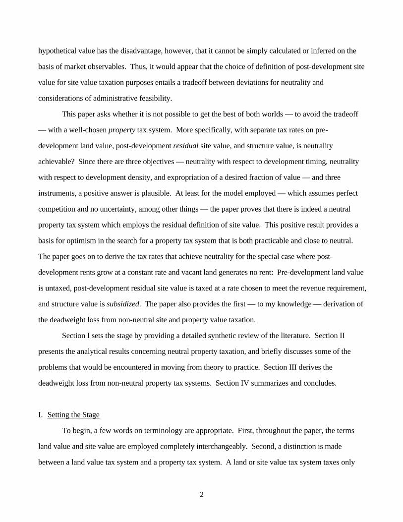
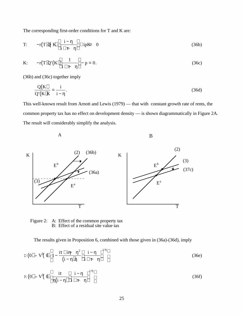
This well-known result from Arnott and Lewis (1979) — that with constant growth rate of rents, the

common property tax has no effect on development density — is shown diagrammatically in Figure 2A.

The result will considerably simplify the analysis.

A

(2) (36b)

(36a)

Eb

Ea

K

T

B

(3)Eb

Ea

(2)

(37c)

K

T

Figure 2: A: Effect of the common property taxB: Effect of a residual site value tax

(3)

The results given in Proposition 6, combined with those given in (36a)-(36d), imply

D =0 0 1

2

( ) ( ) − + −−( )

−+ −

V

i i

i

i

ib

iτ η η

η ηη

τ η

η

(36e)

R =0 0( ) ( )

−( )−

+ −

V

i

i

i

ib

iτ

η ηη

τ η

η

(36f)

26

VpK

i

Q K r

ipKb

i

00( ) =

−( ) ( )

ηη

η

(36g)

T n

ipK

Q K rb =

( ) ( )

1

0ηl (36h)

T T n

i

ia b= + + −

−

1

ητ η

ηl (36i)

Define marginal deadweight loss (MDWL) to be the efficiency loss generated by the marginal dollar

of tax revenue collected. It is straightforward to calculate from (36e) and (36f) that10

MDWL = −( )τ η τ . (36j)

Other values of interest can be calculated straightforwardly from the equations. Note, in accord with

Arnott-Lewis and Figure 2A, that a rise in the tax rate causes development to be postponed.

Two interesting results are given in

Proposition 7 : With the common property tax ( τV = 0 , τ τ τS K= = ) and a constant rental growth rate,

the revenue-maximizing tax rate equals the growth rate of rents, and the marginal deadweight loss from

the tax is τ η τ−( ).

The proof of the first result follows directly from (36f). The result suggests that some common

property tax systems may be “on the wrong side of the Laffer curve”.

b) numerical example

Choose units such that K Q pb b= = = 1, and suppose that11 r i0 03( ) = = . and η = .02 . The

results for several tax rates are recorded in Table 1.

τT K Q L(0)=V(0) D(0) R(0)

0 0 1 1 2 0 0

.01 34.657 1 1 .70711 .23223 1.06066

10 When τ η> , MDWL is negative, since a rise in the tax rate causes deadweight loss to rise and tax revenue to fall.11 r 0( ) is chosen so that in the no-tax situation the land is developed at t=0.

27

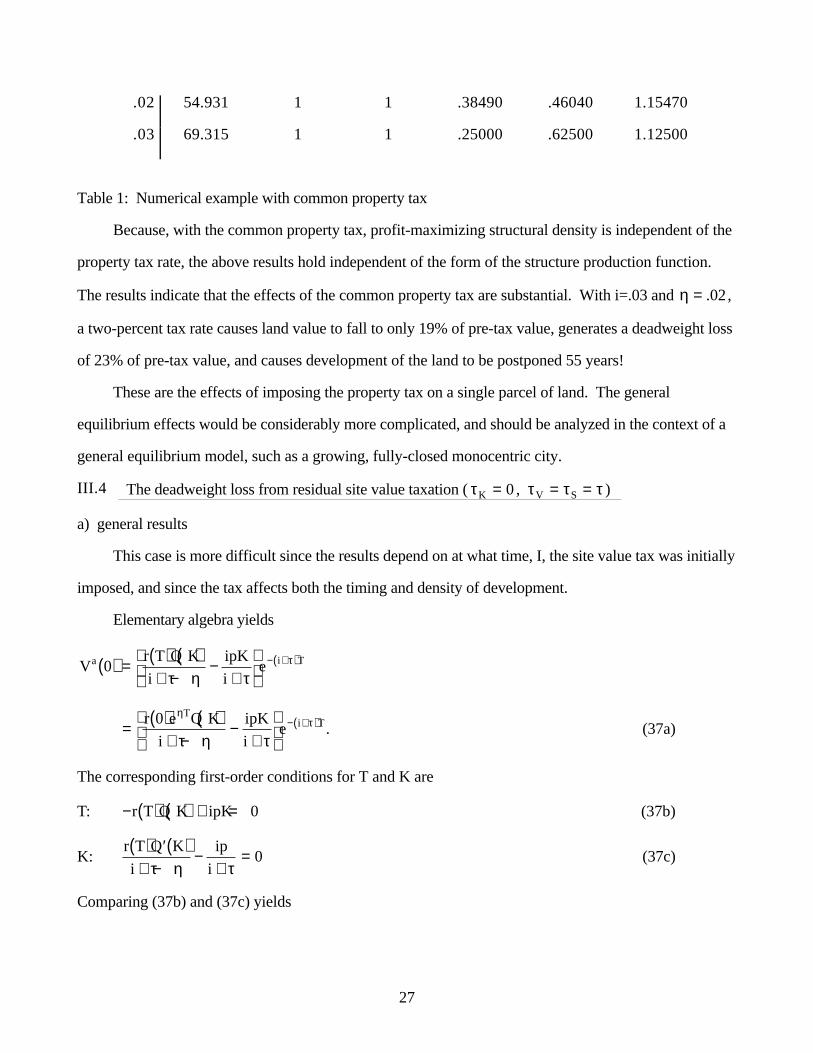
.02 54.931 1 1 .38490 .46040 1.15470

.03 69.315 1 1 .25000 .62500 1.12500

Table 1: Numerical example with common property tax

Because, with the common property tax, profit-maximizing structural density is independent of the

property tax rate, the above results hold independent of the form of the structure production function.

The results indicate that the effects of the common property tax are substantial. With i=.03 and η = .02 ,

a two-percent tax rate causes land value to fall to only 19% of pre-tax value, generates a deadweight loss

of 23% of pre-tax value, and causes development of the land to be postponed 55 years!

These are the effects of imposing the property tax on a single parcel of land. The general

equilibrium effects would be considerably more complicated, and should be analyzed in the context of a

general equilibrium model, such as a growing, fully-closed monocentric city.

III.4 The deadweight loss from residual site value taxation ( τK = 0 , τ τ τV S= = )

a) general results

This case is more difficult since the results depend on at what time, I, the site value tax was initially

imposed, and since the tax affects both the timing and density of development.

Elementary algebra yields

Vr T Q K

i

ipK

iea i T0( ) = ( ) ( )

+ −−

+

− +( )τ η τ

τ

= ( ) ( )+ −

−+

− +( )r e Q K

i

ipK

ie

Ti T0 η

τ

τ η τ. (37a)

The corresponding first-order conditions for T and K are

T: − ( ) ( ) + =r T Q K ipK 0 (37b)

K:r T Q K

i

ip

i

( ) ′( )+ −

−+

=τ η τ

0 (37c)

Comparing (37b) and (37c) yields

28

Q K

Q K K

i

i

( )′( )

= ++ −

ττ η

. (37d)

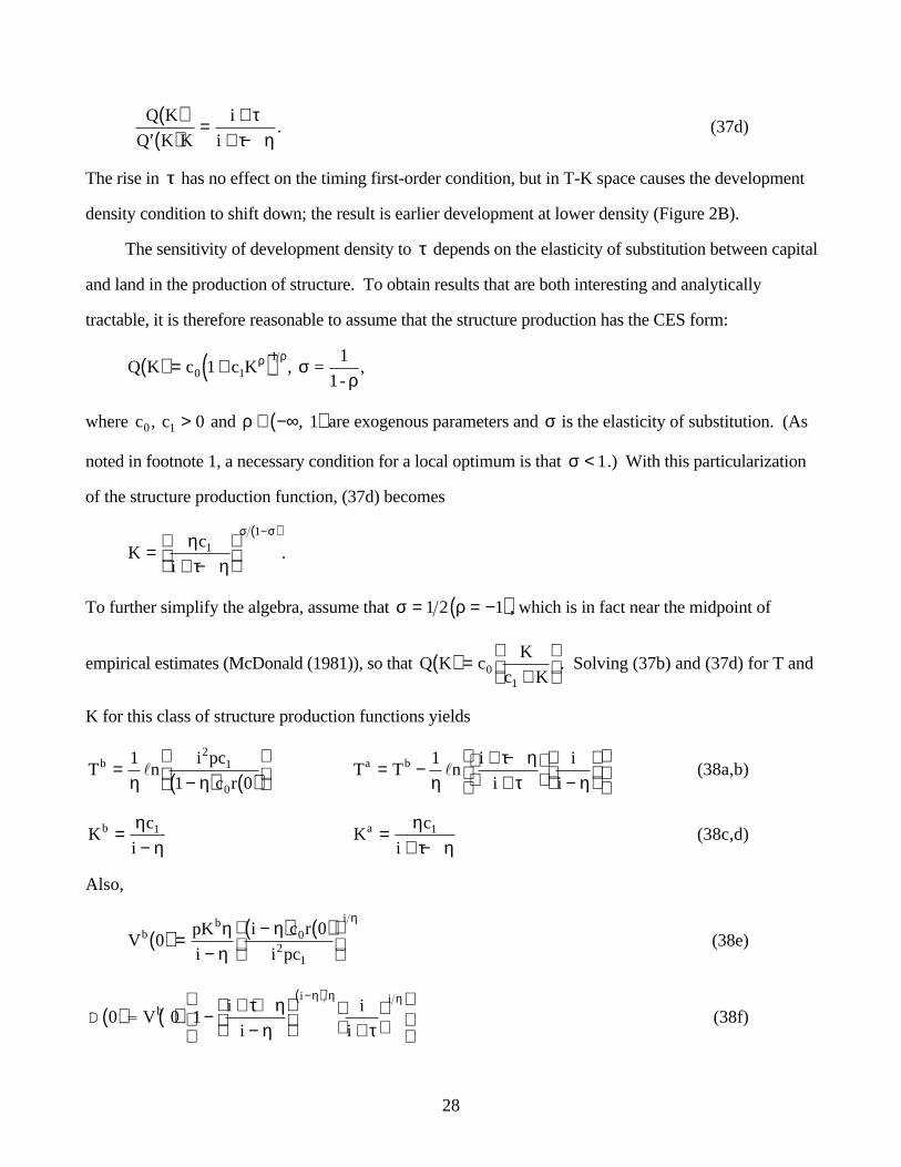
The rise in τ has no effect on the timing first-order condition, but in T-K space causes the development

density condition to shift down; the result is earlier development at lower density (Figure 2B).

The sensitivity of development density to τ depends on the elasticity of substitution between capital

and land in the production of structure. To obtain results that are both interesting and analytically

tractable, it is therefore reasonable to assume that the structure production has the CES form:

Q K c c K( ) = +( )0 1

11 ρ ρ

σρ

, =1

1-,

where c0 0, c1 > and ρ ∈ −∞( ), 1 are exogenous parameters and σ is the elasticity of substitution. (As

noted in footnote 1, a necessary condition for a local optimum is that σ < 1.) With this particularization

of the structure production function, (37d) becomes

Kc

i=

+ −

−( )ητ η

σ σ1

1

.

To further simplify the algebra, assume that σ ρ= = −( )1 2 1 , which is in fact near the midpoint of

empirical estimates (McDonald (1981)), so that Q K cK

c K( ) =

+

0

1

. Solving (37b) and (37d) for T and

K for this class of structure production functions yields

T n

i pc

c rb =

−( ) ( )

1

1 0

21

0η ηl

T T n

i

i

i

ia b= − + −

+

−

1

ητ η

τ ηl (38a,b)

Kc

ib =

−η

η1 K

c

ia =

+ −ητ η

1 (38c,d)

Also,

VpK

i

i c r

i pcb

b i

000

21

( ) =−

−( ) ( )

ηη

ηη

(38e)

D =0 0 1( ) ( ) − + +

−

+

−( )V

i

i

i

ib

i iτ ηη τ

η η η

(38f)

29

R =0 0 1( ) ( ) + −

−

+

−

+

−( )− −( )V

i

i

i

i

i

ieb

i iT Iaτ η

η τ τ

η η ητ

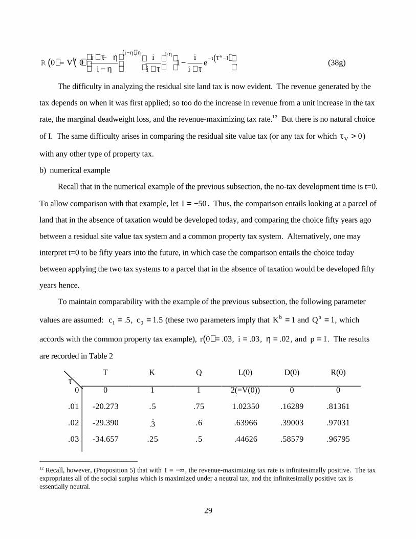
. (38g)

The difficulty in analyzing the residual site land tax is now evident. The revenue generated by the

tax depends on when it was first applied; so too do the increase in revenue from a unit increase in the tax

rate, the marginal deadweight loss, and the revenue-maximizing tax rate.12 But there is no natural choice

of I. The same difficulty arises in comparing the residual site value tax (or any tax for which τV > 0)

with any other type of property tax.

b) numerical example

Recall that in the numerical example of the previous subsection, the no-tax development time is t=0.

To allow comparison with that example, let I = −50 . Thus, the comparison entails looking at a parcel of

land that in the absence of taxation would be developed today, and comparing the choice fifty years ago

between a residual site value tax system and a common property tax system. Alternatively, one may

interpret t=0 to be fifty years into the future, in which case the comparison entails the choice today

between applying the two tax systems to a parcel that in the absence of taxation would be developed fifty

years hence.

To maintain comparability with the example of the previous subsection, the following parameter

values are assumed: c1 5= . , c0 1 5= . (these two parameters imply that Kb = 1 and Qb = 1, which

accords with the common property tax example), r 0 03( ) = . , i = .03, η = .02 , and p = 1. The results

are recorded in Table 2

τT K Q L(0) D(0) R(0)

0 0 1 1 2(=V(0)) 0 0

.01 -20.273 .5 .75 1.02350 .16289 .81361

.02 -29.390 .3 .6 .63966 .39003 .97031

.03 -34.657 .25 .5 .44626 .58579 .96795

12 Recall, however, (Proposition 5) that with I = −∞ , the revenue-maximizing tax rate is infinitesimally positive. The taxexpropriates all of the social surplus which is maximized under a neutral tax, and the infinitesimally positive tax isessentially neutral.

30

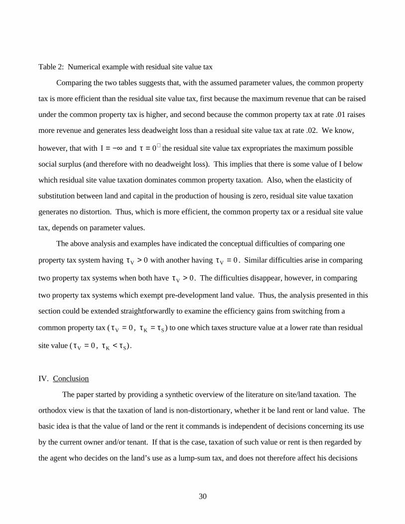
Table 2: Numerical example with residual site value tax

Comparing the two tables suggests that, with the assumed parameter values, the common property

tax is more efficient than the residual site value tax, first because the maximum revenue that can be raised

under the common property tax is higher, and second because the common property tax at rate .01 raises

more revenue and generates less deadweight loss than a residual site value tax at rate .02. We know,

however, that with I = −∞ and τ = +0 the residual site value tax expropriates the maximum possible

social surplus (and therefore with no deadweight loss). This implies that there is some value of I below

which residual site value taxation dominates common property taxation. Also, when the elasticity of

substitution between land and capital in the production of housing is zero, residual site value taxation

generates no distortion. Thus, which is more efficient, the common property tax or a residual site value

tax, depends on parameter values.

The above analysis and examples have indicated the conceptual difficulties of comparing one

property tax system having τV > 0 with another having τV = 0 . Similar difficulties arise in comparing

two property tax systems when both have τV > 0 . The difficulties disappear, however, in comparing

two property tax systems which exempt pre-development land value. Thus, the analysis presented in this

section could be extended straightforwardly to examine the efficiency gains from switching from a

common property tax ( τV = 0 , τ τK S= ) to one which taxes structure value at a lower rate than residual

site value ( τV = 0 , τ τK S< ).

IV. Conclusion

The paper started by providing a synthetic overview of the literature on site/land taxation. The

orthodox view is that the taxation of land is non-distortionary, whether it be land rent or land value. The

basic idea is that the value of land or the rent it commands is independent of decisions concerning its use

by the current owner and/or tenant. If that is the case, taxation of such value or rent is then regarded by

the agent who decides on the land’s use as a lump-sum tax, and does not therefore affect his decisions

31

concerning its use. No contributor to the modern, mainstream literature on the subject disputes this

view. The disagreement instead centers on how land should be valued for property tax purposes after it

has been developed — when there is a durable and immobile structure on the site. Since there is no

market for such land, its value is not logically determinable. There are two broad points of view

concerning how the value developed land should be imputed for property tax purposes. Defenders of the

orthodoxy argue that land value should be defined in such a way that its taxation is neutral. There are

many ways this can be done. One such definition was treated, raw site value — what the site would sell

for if it were undeveloped, even after it has in fact been developed. The problem with using this

definition is that post-development raw site value would be so difficult to estimate that the resulting tax

system would be inequitable, capricious, and subject to abuse. The revisionists have employed an

alternative definition of land value for a built-on site: property value minus structure value, which was

termed residual site value. Property value can be estimated using current assessment practice based on

hedonic analysis, while structure value can be estimated by applying an estimated depreciation rate to

original construction costs. Estimating residual site value would therefore be relatively easy. However,

using residual site value as a basis for taxation violates neutrality; in particular, holding fixed

development time, it discourages density.

Reasonable men may differ concerning which of the two broad approaches to site value taxation

is preferable. I came down on the side of residual site value taxation. Vickrey, whose logic is always

impeccable, favored a definition which comes as close as is administratively feasible to preserving

neutrality.

This paper contributed to the revisionist literature. The revisionists have demonstrated that

residual site value tax is distortionary, but have not taken the next step of asking the question: Is it

possible to design a property tax system employing the residual definition of site value on built-on land

that is neutral? That was the central question addressed in this paper.

A property tax system was defined as a triple of linear taxes: a tax on pre-development land value

at rate τV , a tax on post-development residual site value at rate τS , and a tax on post-development

structure value at rate τK . To address the question, a partial equilibrium model was employed which

32

looked at a single developable site. The simplifying assumptions were made that once a site is developed

at a particular density it remains at that density forever, and that the rent on undeveloped land is zero.

The main result was that for this model there is indeed a combination of the three tax rates that raises a

given level of discounted tax revenues and achieves neutrality. The basic intuition is simple. The

government has three objectives — not distorting the development timing decision, not distorting the

development density condition, and extracting a pre-determined proportion of value — and three

instruments to achieve these objectives. This intuition suggests that the neutrality result extends to

considerably more realistic models than the one employed in this paper.

The paper then calculated the three tax rates that achieve neutrality for the special case in which

the rental growth rate is constant over time. The tax rate on pre-development land value should be zero,

the tax rate of post-development residual site value should be set so as to achieve the desired

expropriation of value, and the structure value tax rate should be negative. One intuition is that, under

the assumptions made, this property tax system is equivalent to a tax on net site rent at a time-invariant

rate, which was earlier shown to be neutral.

The paper then briefly discussed the relevance of the theoretical results for the design of practical

property tax systems, taking into account considerations of informational and administrative feasibility,

and of political acceptability. Two general points were made. The first was that the model requires

considerable elaboration, and that the neutral property tax system generated by any theoretical model

would need to be extensively adapted for practical application. The second was that, these cautions

notwithstanding, it should be possible to design a practicable property tax system that comes close to

achieving neutrality. A sample system was put forward as a basis for discussion: Tax exemption for

land prior to development; residual site value taxation after development, with a structure investment tax

credit being used to offset the depressing effect of residual site value taxation on development density.

The paper went on to derive the deadweight loss associated with non-neutral site value and

property value tax systems. Two particularly noteworthy results were obtained. The first was that a tax

on pre-development land value at an infinitesimal rate, applied from infinitely far in the past up to

development time, is not only neutral but achieves full expropriation of value. The second was that,

33

when structure rents grow at a constant rate, the common property tax system — which (with zero

agricultural rent) applies a zero tax rate to pre-development land value and equal tax rates to post-

development residual site and structure values — has a revenue-maximizing tax rate equal to the growth

rate of rents.

One final remark. The literature on property taxation, to which the paper has contributed, has

evolved largely independently of other important developments in public economics. There is an

extensive literature on neutral capital taxation (e.g., Samuelson (1964), King and Fullerton (1984)). The

two literatures should be integrated, not only to develop results on neutral capital c property taxation, but

also to investigate second-best efficient property taxation when capital taxation is distorted, and vice

versa. There is also an extensive literature on the design of optimal tax systems, which takes into

account the equity-efficiency tradeoffs produced by asymmetries in information. It is time for the

property tax to be considered as one component of a broad tax system rather than being examined in

isolation.

34

BibliographyArnott, R.J., and F.D. Lewis. “The Transition of Land to Urban Use”. Journal of Political Economy 87

(1979), 161-169.

Bentick, B.L. “The Impact of Taxation and Valuation Practices on Timing and Efficiency of Land Use”.Journal of Political Economy 87 (1979), 858-868.

Capozza, D., and Y. Li. “The Intensity and Timing of Investment: The Case of Land”. AmericanEconomic Review 84 (1994), 889-904.

Chinloy, P. “The Estimation of Net Depreciation Rates on Housing”. Journal of Urban Economics 6(1979), 432-443.

George, H. Progress and Poverty (1879). New York: Robert Schalkenback Foundation, 1970.

Kanemoto, Y. “Housing as an Asset and the Effects of Property Taxation on the ResidentialDevelopment Process”. Journal of Urban Economic 17 (1985), 145-166.

King, M. and D. Fullerton, eds. The Taxation of Income from Capital , Chapter 2. Chicago, IL:University of Chicago Press, 1984.

Ladd, H.F. Local Government Tax and Land Use Policies in the United States: Understanding theLinks , Ch. 2. Cheltenham, U.K.: Edward Elgar, 1997.

McDonald, J. “Capital-land Distribution in Urban Housing: A Survey of Empirical Estimates.” Journalof Urban Economics 9 (1981) 190-211.

Mills, D.E. “The Non-Neutrality of Land Value Taxation” National Tax Journal 34 (1981), 125-129.

Mills, D.E. “Reply to Tideman”. National Tax Journal 35 (1982), 115.

Netzer, D. “What Do We Need to Know about Land Value Taxation?” (1997), mimeo.

Samuelson, P. “Tax Deductibility of Economic Depreciation to Insure Invariant Valuations”. Journal ofPolitical Economy 62 (1964), 604-606.

Shoup, D. “The Optimal Timing of Urban Land Development”. Papers of the Regional ScienceAssociation 25 (1970), 33-44.

Skouras, A. “The Non-neutrality of Land Taxation”. Public Finance 30 (1978), 113-134.

Sweeney, J. “A Commodity Hierarchy Model of the Rental Housing Market”. Journal of UrbanEconomics 1 (1974), 288-323.

Tideman, N.T. “A Tax on Land Is Neutral”. National Tax Journal 35 (1982), 109-111.

Turnbull, G.K. “Property Taxes and the Transition of Land to Urban Use”. Journal of Real EstateFinance and Economics 1 (1988), 393-403.

Vickrey, W.S. “Defining Land Value for Taxation Purposes”, in The Assessment of Land Value , D.M.Holland, ed. Milwaukee, WI: University of Wisconsin Press, 1970.

Wildasin, D.E. “More on the Neutrality of Land Taxation”. National Tax Journal 35 (1982), 105-108.

35

Appendix 1Proof of Result 3 :

Prior to development, raw site value equals the value of the vacant land, V t( ) . After

development, raw site value equals the value of the land were it still undeveloped.

Using (6), the value of vacant land for t<T is

V t

K Tr u Q K e du pKe u e du

Ti u t i T t

ti u t( ) = ( ) ( ) − − ( )[ ]∞ − −( ) − −( ) ∞ − −( )∫ ∫max

,τS S

= ( ) ( ) − − ( ) − ( )[ ]∞ − −( ) − −( ) − −( ) − −( )∞

∫ ∫ ∫max,K T

r u Q K e du pKe V u e du u e duT

i u t i tt

T i u t i u tT

τ τ τS S Φ . (A1.1a)

The value of the land at t T≥ if, hypothetically, it were still undeveloped is

Φ Φt

K t T tr u Q K t e du pK t e u e du

T t

i u t i T t t

t

i u t( ) =( ) ( )

( ) ( )( ) − ( ) − ( )

( )

∞ − −( ) − ( )−( ) ∞ − −( )∫ ∫maxˆ , ˆ

ˆ ˆˆ

ˆτS , (A1.1b)

where T t( ) is the profit-maximizing time to develop the land13 conditional on its being undeveloped at

time t, and K (t) is defined analogously.

Since the developer in fact develops at t=T, post-development raw site value is independent of his

actions. Accordingly, he views post-development raw site value tax payments as lump-sum taxes. Pre-

development raw site value, meanwhile, is the market value and does depend on the profit-maximizing T

and K.

Define Z(T) to be the sum of post-development raw site value tax payments, discounted to T:

Z T u e dui u T

T( ) = ( ) − −( )∞

∫τS Φ . (A1.2a)

Substituting (A1.2a) into (A1.1a) yields

V t

K Tr u Q K e du pKe V u e du Z T e

Ti u t i T t

t

T i u t i T t( ) = ( ) ( ) − − ( ) − ( )[ ]∞ − −( ) − −( ) − −( ) − −( )∫ ∫max,

τS . ( A a1 1. ′)

Differentiation with respect to t gives

V i V= +( )τS

36

and

V t

K Tr u Q K e du pK Z T e

T

i u T i T t( ) = ( ) ( ) − −[ ]∞ − −( ) − +( ) −( )∫max,

( ) τS . ( A a1 1. ′′ )

It is easy to see from ( A a1 1. ′′ ) that the first-order condition for density is independent of τS . The first-

order condition for development timing is

− +( ) ( ) − ( ) ( ) + ( ) ( ) − ′( ) =− −( )∞∫i V T r T Q K i r u Q K e du Z Ti u T

TτS 0. (A1.3a)

Substituting ( A a1 1. ′′ ) evaluated at T into (A1.3a) yields

− ( ) − ( ) ( ) + + ( ) − ′( ) =τS V T r T Q K ipK iZ T Z T 0 . (A1.3b),

Finally, substituting ′( ) = − ( ) + ( )Z T T iZ TτS Φ (from (A1.2a)) and V T T( ) = ( )Φ , (A1.3b) reduces to

the first-order condition without the raw site value tax. Thus, the raw site value tax is neutral. þ

To understand this result, consider first the development density condition. Turn to ( A a1 1. ′).

For the development density condition to be unaffected by the site value tax, the derivative of the last two

terms with respect to K must equal zero. The derivative of the second last term equals zero since V(u) is

the maximized value of discounted net revenue with respect to K, implying ∂

∂V u

K

( ) = 0 . And the

derivative of the last term equals zero since, with development time fixed, post-development raw site

value tax payments are independent of development density. Consider next the development timing

condition. For this condition too to be unaffected by the site value tax, the derivative of the last two

terms of ( A a1 1. ′) with respect to T must equal zero. Using (A1.2a), this derivative is

− ( ) − ( ) − ( )( )− −( ) − −( )∫τ ∂

∂τS S

V u

Te du V T T ei u t i T t

t

TΦ .

The first term equals zero since V u( ) is the maximized value of discounted net revenue with respect to T,

implying ∂

∂V u

T

( ) = 0 , and the second equals zero since V T T( ) = ( )Φ .

13 In a smoothly growing economy, the land would be developed immediately.

37

Appendix 2

Relationship between τV , τS, and τK

(Not for Publication)

The two neutrality conditions are (21b) and (22). We shall derive the revenue condition. Then

we shall have three equations in three unknowns, and we shall investigate the properties of the equation

system. We assume throughout that τS i> − .

a) the revenue condition

To simplify the notation somewhat, let t=0 denote the time at which the land value tax is first

applied.

Let R ( )T denote the value of revenue collected, evaluated at time T:

R T V t e dt pKe dt S t e dtV

T i T tK

i t T

T Si t T

T( ) = ( ) + + ( )∫ ∫ ∫−( ) − −( )∞ − −( )∞

τ τ τ0

. (A2.1)

From (15)

τ τ τ

τ

VT i T t

VT i T t i T t

T

V t e dt V T e e dt

V T e

V

V

( ) = ( )

= ( ) −( )∫ ∫−( ) − +( ) −( ) −( )

−0 0

1 .(A2.2)

From (12)

τ τSi t T

T KT

i t TS t e dt S T rQ i pK e dt( ) = − ( ) + − +( )( )− −( )∞ ∞ − −( )∫ ∫ . (A2.3)

And

pKe dtpK

iT

i t T∞ − −( )∫ = . (A2.4)

Combining (A2.1) - (A2.4) yields

R T V T e

pK

iS T rQ i pK e dtVT K

KTi t T( ) = ( ) −( ) + − ( ) + − +( )( )− ∞ − −( )∫1 τ τ τ

= − ( ) + − ( ) ( )− ∞ − −( )∫V T e rQe dt pK S T V TVTT

i t Tτ (using = )

= − − +( )( )

+ −∞ − +( ) −( ) − ∞ − −( )∫ ∫rQ i pK e dt e rQe dt pKKT

i t T TT

i t TS Vτ τ τ . (using (15b)) (A2.5)

38

b) the three equations

Define

A r t e dt B r t e dti t TST

i t T

TS≡ ( ) ( ) ≡ ( )− −( )∞ − +( ) −( )∞

∫ ∫τ τ . (A2.6)

Rewrite the three equations using (A2.6). Eq. (19) becomes

A i i BK S S+( ) − +( ) ( ) =τ τ τ 0 . (A2.7)

Equation (18b) becomes

τ τ τ τ ττK S V S

K

S

pK B Qi

ipK+ −( ) ( ) − +

+

= 0 . (A2.8)

And eq. (A2.5) becomes

R T B Q

i

ipK e AQ pKS

K

S

TV( ) = − ( ) − ++

+ − =−τ τ

ττ 0 . (A2.9)

Now substitute (A2.7) into (A2.8) and (A2.9). Then the three equations can be written as

A i i BK S S+( ) − +( ) ( ) =τ τ τ 0 (A2.7)

τ τ τ ττK S V

K

S

pKi

iAQ pK+ −( ) +

+

−( ) = 0 (A2.8´)

R T AQ pK

i

ieK

S

TV( ) = −( ) − ++

−1ττ

τ . (A2.9´)

Note that AQ-pK is site value at development time in the pre-tax situation. Thus,

ε ≡ ( )

−R T

AQ pK(A2.10)

is the ratio of the value of tax collected evaluated at development time to the pre-tax site value at

development time, which is the measure employed of the proportion of site value expropriated through

the tax. Define η implicitly as

i r T A− = ( )η . (A2.11)

Then the development timing condition in the pre-tax situation (eq. 2) can be written as

A i Q ipK−( ) − =η 0 , so that

39

AQ pK pKi

i

pK

i− =

−−

=−˜

˜

˜ηηη

1 . (A2.12)

Using (A2.10) and (A2.12), (A2.7), (A2.8´), and (A2.9´) can be rewritten as

A i i BK S S+( ) − +( ) ( ) =τ τ τ 0 (A2.7)

τ τ τ ττ

ηηK S V

K

S

i

i i+ −( ) +

+

−

=˜

˜0 (A2. ′′8 )

1 0− ++

− =−i

ieK

S

TVττ

ετ . (A2. ′′9 )

This set of three equations characterizes the set of ( τV , τS , and τK ) that achieve neutrality and

expropriate a proportion ε of site value.

c) τ τ τK K S= ( )

Observe that (A2.7) gives τK as a function of τS . When τS=0, A=B( τS) so that τK =0; thus,

τK ( τS) passes through the origin in τS- τK space. Also,

d

d

B i B

AK

S A

S S Sττ

τ τ τ( . )2 7

= ( ) + +( ) ′( ). (A2.13)

From (A2.6), defining u=t-T, B r u e duSi uSτ τ( ) = ( ) − +( )∞

∫0, so that

′( ) = − ( ) − +( )∞∫B r u ue duS

i uSτ τ0

= ( )+

− +( )

+( ) <− +( ) ∞

∞ − +( )∫r u ue

i

ru r

ie du

i u

S S

i uS

S

ττ

τ τ0

00

˙ (integration by parts). (A2.14)

Substituting (A2.14) into (A2.13) yields

d

d Arue duK

S A

i uSττ

τ

( . )

˙2 7

0

1= −∞ − +( )

∫ . (A2.15)

This is ambiguous in sign. In a growing economy, however, one expects r > 0, except for downturns

in the business cycle. Thus, “normally” d

dK

SA

ττ

< 02 7( . )

.

40

(AS-1): rue du u t T ii uS

00

∞ − +( )∫ > ≡ > −

ττ for - and S

Proposition A1 : Under (AS-1), d

dK

SA

ττ

< 02 7( . )

.

Differentiating (A2.15) with respect to τS gives

d

d Aru e duK

S A

i uS2

22 7

2

0

1ττ

τ

( . )

˙=∞ − +( )

∫ .

(AS-2): ru e du u t T ii uS2

00

∞ − +( )∫ > ≡ > −

ττ for - and S

Proposition A2 : Under (AS-2), d

dK

SA

2

2 2 70

ττ

>( . )

.

Figure A1 plots the relationship between τK and τS under (AS-1) and (AS-2).

τ τ τK K S= ( )

τK

τS

Figure A1

d) τ τ τV V S= ( )

Substituting (A2.7) into (A2. ′′9 ) gives an implicit relationship between τV and τ τ τ τS V V S= ( )( ):

1 0− ( ) − =−B

AeS V Tτ

ετ . (A2.16)

Differentiating (A2.16) yields

d

d

B

BTV

S A

ττ ( . )2 16

0= ′ < (A2.17)

Also,

41

d

d

B

BT

B

B TV

S A

2

22 16

2

2

ττ ( . )

= ′′ −′( )

,

which is in general ambiguous in sign.

Figure A2 plots this relationship between τV and τS .

τS

Figure A2τ τV S( )

ε0

ε1

τV

ε ε1 0>

Loci further northeast from the origin correspond to higher levels of expropriation.

e) τ τ τV V S= ( )

Substituting (A2.7) into (A2. ′′8 ) gives another relationship between τV and τ τ τ τS V V S= ( )( ):

i B

Ai

B

A iS S

S VS+( ) ( ) −

+ −( ) ( )−

=τ τ

τ ττ η

η˜

˜0

or

τη

η ττ

ηVs

S

i i A

B

i=−( )

− ( )

+

˜

˜ ˜1 . (A2.18)

Note first that when τS=0, A=B, which implies that τV =0. Thus, τ τV S( ) passes through the origin in

τ τS K− space. Also,

d

d

ii

A

BBV

S A

ττ η

η( . ) ˜

˜2 18

2 1= −( ) ′ +

. (A2.19)

Now define η τS( ) implicitly by

B r u e du r e dui u i uS S S= ( ) = ( )− +( )∞ − + − ( )( )∞∫ ∫τ τ η τ0 0

0ˆ

(A2.20a)

42

and ˆη τS( ) implicitly by

′ = − ( ) = − ( )− +( )∞ − + − ( )( )∞∫ ∫B r u ue du r ue dui u i u

S S Sτ τ η τ

0 00

ˆ. (A2.20b)

Both η τS( ) and ˆη τS( ) are weighted average rental growth rates. Because ′B contains the extra u inside

the integral, the calculation of ˆη τS( ) puts more weight on later periods than does η τS( ). Thus

ˆ ˆη τ η τS S( )>< ( ) if the rental growth rate

falls

rises

over time. Substituting (A2.20a), (A2.20b), and the

definitions of η and ˆη into (A2.19) yields

d

d

i i

iV

S A

S S

S S

ττ η

τ η τ

τ η τ( . ) ˜

ˆ

ˆ2 18

2

1= −+ − ( )+ − ( )

+

. (A2.21)

If rental growth is exponential, η τS( )= ˆη τS( ) so that d

dV

S A

ττ ( . )2 18

0= . If rental growth falls

rises

over time, d

dV

S A

ττ ( . )2 18

0>< , and when rental growth fluctuates over time τ τV S( ) need not be monotonic.

These results are sufficiently important that we record them.

Proposition A3 : d

dV

S A

ττ ( . )2 18

has the same sign as ˆ ˆη τ η τS S( ) − ( ) . Thus, if ˆ ˆη τ η τS S( )>=<

( ) for all τS , then

τ τV S( ) is

monotonically increasing

constant

monotonically decreasing

.

Figure A3 plots τ τV S( ) ((A2.16)) and τ τV S( ) ((A2.18)) for five cases.

43

τS

τV

(A2.16)

(A2.18)

I

τS

τV

(A2.16)

(A2.18)II

τS

τV

(A2.16)

(A2.18)

III

τS

τV

(A2.16)

(A2.18)IV

τS

τV

(A2.16)

(A2.18)

V

(coincides withhorizontal axis)

Case I depicts the situation with exponential rental growth. Neutrality entails τS>0, τV =0, and (from

Figure A.1 since (AS-1) is satisfied) τK <0. Case II depicts a maturing city in which the growth rate of

rents is positive but falling over time. Neutrality entails τS>0, τV >0, and τK <0. Cases III and IV

depict incipient boom towns in which the rental growth rate is increasing over time. In Case III, τS>0,

τV <0, and (when (AS-1) is satisfied) τK <0; and in case IV, τS<0, τV >0, and (when (AS-1) is satisfied)

44

τK >0. Case V demonstrates the possibility of multiple neutral property tax systems satisfying a

particular revenue requirement.

The above line of analysis can be extended straightforwardly to more complex situations, for

example where the interest rate varies over time and where there is technical change in construction. The

extension to treat uncertainty — for example where the time path of rents follows a stochastic process —

will be more difficult.

Appendix 1

Proof of Result 3 :

Prior to development, raw site value equals the value of the vacant land, V t( ) . After

development, raw site value equals the value of the land were it still undeveloped.

Using (6), the value of vacant land for t<T is

V t

K Tr u Q K e du pKe u e du

Ti u t i T t

ti u t( ) = ( ) ( ) − − ( )[ ]∞ − −( ) − −( ) ∞ − −( )∫ ∫max

,τS S

= ( ) ( ) − − ( ) − ( )[ ]∞ − −( ) − −( ) − −( ) − −( )∞

∫ ∫ ∫max,K T

r u Q K e du pKe V u e du u e duT

i u t i tt

T i u t i u tT

τ τ τS S Φ . (8a)

The value of the land at t T≥ if, hypothetically, it were still undeveloped is

Φ Φt

K t T tr u Q K t e du pK t e u e du

T t

i u t i T t t

t

i u t( ) =( ) ( )

( ) ( )( ) − ( ) − ( )

( )

∞ − −( ) − ( )−( ) ∞ − −( )∫ ∫maxˆ , ˆ

ˆˆ

ˆτS , (8b)

where T t( ) is the profit-maximizing time to develop the land1 conditional on its being undeveloped

at time t, and K (t) is defined analogously.

Since the developer in fact develops at t=T, post-development raw site value is independent

of his actions. Accordingly, he views post-development raw site value tax payments as lump-sum

taxes. Pre-development raw site value, meanwhile, is the market value and does depend on the

profit-maximizing T and K.

Define Z(T) to be the sum of post-development raw site value tax payments, discounted to

T:

Z T u e dui u T

T( ) = ( ) − −( )∞

∫τS Φ . (9a)

Substituting (9a) into (8a) yields

V t

K Tr u Q K e du pKe V u e du Z T e

Ti u t i T t

t

T i u t i T t( ) = ( ) ( ) − − ( ) − ( )[ ]∞ − −( ) − −( ) − −( ) − −( )∫ ∫max,

τS . (8 ′a )

Differentiation with respect to t gives

V i V= +( )τS

and

V t

K Tr u Q K e du pK Z T e

T

i u T i T t( ) = ( ) ( ) − −[ ]∞ − −( ) − +( ) −( )∫max,

( ) τS (8 ′′a )

It is easy to see from (8 ′′a ) that the first-order condition for density is independent of τS . The

first-order condition for development timing is

− +( ) ( ) + − ( ) ( ) + ( ) ( ) − ′( )[ ] =− −( )∞ − −( ) −( )∫i V t r T Q K i r u Q K e du Z T ei u T

T

i T tτ τS

S 0 . (10a)

Substituting (8 ′′a ) into (10a) and evaluating at t=T yields

− ( ) − ( ) ( ) + + ( ) − ′( ) =τS V T r T Q K ipK iZ T Z T 0 . (10b),

Finally, substituting ′( ) = − ( ) + ( )Z T T iZ TτS Φ (from (9a)) and V T T( ) = ( )Φ , (10b) reduces to

the first-order condition without the raw site value tax. Thus, the raw site value tax is neutral. þ

To understand this result, consider first the development density condition. Turn to (8 ′a ).

For the development density condition to be unaffected by the site value tax, the derivative of the

last two terms with respect to K must equal zero. The derivative of the second last term equals

zero since V(u) is the maximized value of discounted net revenue with respect to K, implying

∂∂V u

K

( ) = 0 . And the derivative of the last term equals zero since, with development time fixed,

post development raw site value tax payments are independent of development density. Consider

next the development timing condition. For this condition too to be unaffected by the site value

tax, the derivative of the last two terms of (8 ′a ) with respect to T must equal zero. Using (9a), this

derivative is

− ( ) − ( ) − ( )( )− −( ) − −( )∫τ ∂

∂τS S

V u

Te du V T T ei u t i T t

t

TΦ .

The first term equals zero since V u( ) is the maximized value of discounted net revenue with

1 In a smoothly growing economy, the land would be developed immediately.

respect to T, implying ∂

∂V u

T

( ) = 0 , and the second equals zero since V T T( ) = ( )Φ .