NEW ALGORITHM FOR THE TRIANGULATION OF INPUT-OUTPUT TABLES AND THE LINEAR ORDERING PROBLEM By BRUNO H. CHIARINI A THESIS PRESENTED TO THE GRADUATE SCHOOL OF THE UNIVERSITY OF FLORIDA IN PARTIAL FULFILLMENT OF THE REQUIREMENTS FOR THE DEGREE OF MASTER OF SCIENCE UNIVERSITY OF FLORIDA 2004
Transcript
NEW ALGORITHM FOR THE TRIANGULATION OF INPUT-OUTPUTTABLES AND THE LINEAR ORDERING PROBLEM
By
BRUNO H. CHIARINI
A THESIS PRESENTED TO THE GRADUATE SCHOOLOF THE UNIVERSITY OF FLORIDA IN PARTIAL FULFILLMENT
OF THE REQUIREMENTS FOR THE DEGREE OFMASTER OF SCIENCE
UNIVERSITY OF FLORIDA
2004
ACKNOWLEDGMENTS
I would like to thank all the people who played a role in my career at the
University of Florida (Elif Akcalı, Donald Hearn, and Edwin Romeijn, among
others). I specially thank my committee members (Stanislav Uryasev and Panos
Pardalos) for their time and candid review of my thesis.
There is somebody who will forever have a special place in my heart: Panos
M. Pardalos. I thank him for all his support and advice throughout my career. I
will miss him, but I am leaving with the hope of having other opportunities to work
together in the future.
The last mention is reserved for some very special people, without whom this
would have been an impossible journey. They have endured ups and downs, and
grown with me to form a stronger nucleus. They are the source from which I pull
strength and wisdom, and the recipients of my work. This work is dedicated to
them. I thank Diane and Gianluca for their eternal love, patience, and support.
4–1 The LOLIB Instances: gap from optimal solution as a percentage isshown as a function of the number of iterations. . . . . . . . . . . . 22
4–2 The LOLIB Instances: gap from optimal solution as a percentage isshown as a function of the time elapsed (seconds). . . . . . . . . . . 22
4–3 Mitchell Instances: gap from optimal solution as a percentage isshown as a function of the number of iterations. . . . . . . . . . . . 23
4–4 Mitchell Instances: gap from optimal solution as a percentage isshown as a function of the time elapsed (seconds). . . . . . . . . . . 23
v
Abstract of Thesis Presented to the Graduate Schoolof the University of Florida in Partial Fulfillment of the
Requirements for the Degree of Master of Science
NEW ALGORITHM FOR THE TRIANGULATION OF INPUT-OUTPUTTABLES AND THE LINEAR ORDERING PROBLEM
By
Bruno H. Chiarini
May 2004
Chair: Panos M. PardalosMajor Department: Industrial and Systems Engineering
Developed by Leontief in the 1930s, input-output models have become an
indispensable tool for economists and policy-makers. They provide a framework
on which researchers can systematically analyze interrelations among sectors of
an economy. In an input-output model, a table is constructed where each entry
represents the flow of goods between each pair of sectors. Special features of the
structure of this matrix are revealed by a technique called triangulation.
Triangulation is shown to be equivalent to the linear ordering problem
(LOP), which is an NP-hard combinatorial optimization problem. Because of
the complexity of the triangulation procedure, it is essential in practice to search
for quick approximate (heuristic) algorithms for the linear ordering problem. In
addition to the triangulation of input-output tables, the LOP has a wide range of
applications in practice, including single-server scheduling and ranking of objects
by pairwise comparisons. However, a higher emphasis is placed on the triangulation
of input-output tables, the original motivation for this work.
Our study developed a new heuristic procedure to find high-quality solutions
for the LOP. The proposed algorithm is based on a Greedy Randomized Adaptive
vi
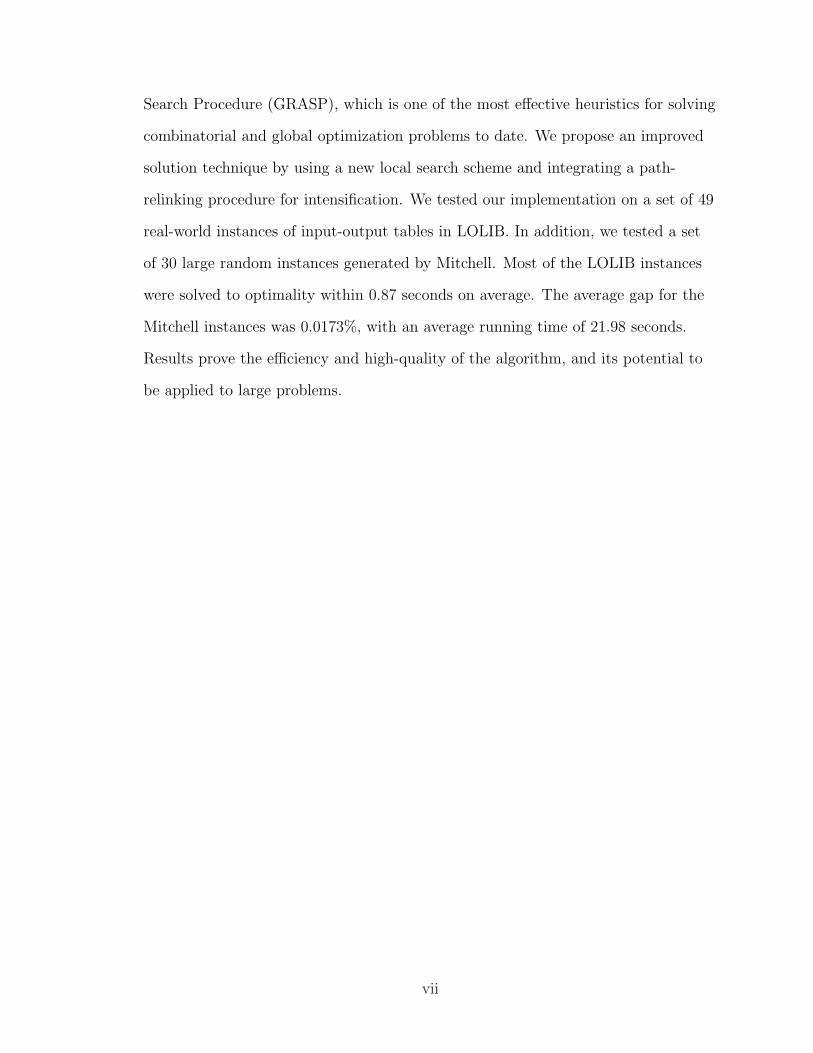
Search Procedure (GRASP), which is one of the most effective heuristics for solving
combinatorial and global optimization problems to date. We propose an improved
solution technique by using a new local search scheme and integrating a path-
relinking procedure for intensification. We tested our implementation on a set of 49
real-world instances of input-output tables in LOLIB. In addition, we tested a set
of 30 large random instances generated by Mitchell. Most of the LOLIB instances
were solved to optimality within 0.87 seconds on average. The average gap for the
Mitchell instances was 0.0173%, with an average running time of 21.98 seconds.
Results prove the efficiency and high-quality of the algorithm, and its potential to
be applied to large problems.
vii
CHAPTER 1INTRODUCTION
The impact of changes of an economic variable can only be analyzed by
understanding the complex series of transactions taking place among the sectors
of an economy. First introduced by Leontief in the early 1930s, input-output
models have become an indispensable tool for economists and policy-makers in
their analysis, providing a systematic description of such interrelations among the
sectors [1].
An input-output model begins by dividing the economy of a country (or
region) into a specified number of sectors. Then a table is constructed, where the
entries are the total transactions between every pair of sectors. The total output
(input) of a sector can be obtained by summing the entries on the corresponding
row (column). The resulting table thus summarizes the interdependence among the
economic sectors.
Structural properties of the input-output tables may not be apparent. A
particular choice in the order of the sectors used in constructing the table might
conceal an otherwise evident structure. These features are revealed by a process
called triangulation, whose objective is to find a hierarchy of the sectors such that
those who are predominantly producers will appear first, while those who are
mainly consumers will appear last.
The economic significance is that it shows how the effects of changes in final
demand propagate through the sectors. Note, however, that in using a hierarchic
ordering, there is an underlying assumption that no flow exists from lower to upper
sectors. In fact, every economy exhibits a certain circularity in the flow of goods—
e.g., the metallurgy industry supplies the vehicle industry with raw metal products,
1
2
while the metallurgy sector needs vehicles as part of the cost of doing business.
Obviously, the flow between any two sectors is hardly symmetric.
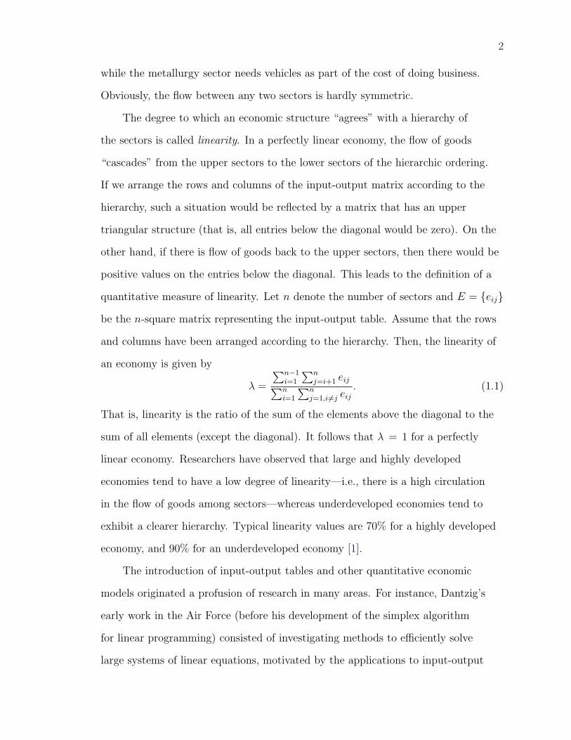
The degree to which an economic structure “agrees” with a hierarchy of
the sectors is called linearity. In a perfectly linear economy, the flow of goods
“cascades” from the upper sectors to the lower sectors of the hierarchic ordering.
If we arrange the rows and columns of the input-output matrix according to the
hierarchy, such a situation would be reflected by a matrix that has an upper
triangular structure (that is, all entries below the diagonal would be zero). On the
other hand, if there is flow of goods back to the upper sectors, then there would be
positive values on the entries below the diagonal. This leads to the definition of a
quantitative measure of linearity. Let n denote the number of sectors and E = {eij}be the n-square matrix representing the input-output table. Assume that the rows
and columns have been arranged according to the hierarchy. Then, the linearity of
an economy is given by
λ =
∑n−1i=1
∑nj=i+1 eij∑n
i=1
∑nj=1,i6=j eij
. (1.1)
That is, linearity is the ratio of the sum of the elements above the diagonal to the
sum of all elements (except the diagonal). It follows that λ = 1 for a perfectly
linear economy. Researchers have observed that large and highly developed
economies tend to have a low degree of linearity—i.e., there is a high circulation
in the flow of goods among sectors—whereas underdeveloped economies tend to
exhibit a clearer hierarchy. Typical linearity values are 70% for a highly developed
economy, and 90% for an underdeveloped economy [1].
The introduction of input-output tables and other quantitative economic
models originated a profusion of research in many areas. For instance, Dantzig’s
early work in the Air Force (before his development of the simplex algorithm
for linear programming) consisted of investigating methods to efficiently solve
large systems of linear equations, motivated by the applications to input-output
3
tables [1, 2]. However, the triangulation problem described next has not been given
much attention.
Triangulation. We have assumed so far the knowledge of a hierarchy
of sectors. Triangulation of an input-output table is the process of finding such
hierarchy among all possible orderings. It is clear from the discussion above
that such ordering most closely resembles an upper triangular matrix, and thus
has the maximum value of λ. Note that every ordering is a permutation of the
sectors, and it is applied to both the rows and columns of the input-output matrix.
Additionally, the denominator of Equation 1.1 is constant for all permutations.
Therefore, we can state the triangulation problem as that of finding a permutation
of the rows and columns, such that the sum of the elements above the diagonal
is maximum. Clearly, this is equivalent to a combinatorial optimization problem,
known as the linear ordering problem (LOP).
Finding such permutation is not an easy task. In fact, the linear ordering
problem is an NP-hard problem, and as such we can only aspire to obtain
approximate solutions. Furthermore, the extent to which input-output methods are
useful depends on the efficiency of the computations. Limited by computational
power, practitioners often must recur to aggregation, with the consequent loss of
information and accuracy, to find optimal solutions within an acceptable time.
Therefore, it is essential in practice to search for quick approximate (heuristic)
algorithms.
In this thesis we propose a new algorithm based on a greedy randomized
adaptive search procedure (GRASP) to efficiently solve the LOP. The algorithm is
integrated with a path-relinking procedure and a new local search scheme.
The remainder of this work is organized as follows. In Chapter 2 we introduce
the LOP, give other applications, and discuss some previous work. In Chapter 3 we
give a detailed implementation of our algorithm, preceded by an introduction
4
describing the GRASP and path-relinking framework. The computational
experimentation is shown in Chapter 4. The thesis concludes with Chapter 5,
where some practical issues are discussed.
CHAPTER 2LINEAR ORDERING PROBLEM
The LOP is an NP-hard combinatorial optimization problem with a wide
range of applications in economics, archaeology, and scheduling. It has, however,
drawn little attention compared to other closely related problems such as the
quadratic assignment problem and the travelling salesman problem.
The LOP can be stated as follows. Consider a set N of n objects and a
permutation π : N → N . Each permutation π = (π(1), π(2), . . . , π(n)) corresponds
one-to-one to a linear ordering of the objects. Let eij, i, j = 1, 2, . . . , n, be the cost
of having i before j in the ordering, and E be the n-square matrix of costs. Then
the linear ordering problem is to find a permutation π that maximizes the total
cost
Z(π) =n−1∑i=1
n∑j=i+1
eπ(i)π(j). (2.1)
Clearly, Equation 2.1 is the sum of the elements above the diagonal of a
matrix A, whose elements aij are those resulting from a permutation π of the
rows and columns of matrix E—i.e., A = XEXT , where X is the permutation
matrix associated with the permutation π [3]. In the context of its application in
economics, we can restate Equation 1.1 as
λ =1
Kmaxπ∈Π
{Z(π)} (2.2)
where Π is the set of all permutations, and K is a positive constant representing
the sum of all the entries in the matrix.
The LOP can also be interpreted as a problem in graphs. Let G(N, A) be a
complete directed graph with node set N and arc set A = {(i, j) : i, j ∈ N ∧ i 6= j}.
5
6
Let eij be the weight of arc (i, j). A spanning acyclic tournament in G induces a
unique linear ordering of the node set N [4]. A tournament is defined as a directed
graph in which each pair of nodes is connected by exactly one arc, which is clearly
necessary since either i is before j or j is before i.
The complexity of the maximum LOP can be easily proven to be NP-hard by
noticing that it is equivalent to the minimum weighted feedback arc set problem on
G, which is known to be NP-hard [5].
The LOP has an interesting symmetry property. If a permutation π =
(π(1), π(2), . . . , π(n)) is an optimal solution to the maximization version, then
the reverse permutation π = (π(n), π(n − 1), . . . , π(1)) is an optimal solution
to the minimization version. In fact, the LOP accepts a trivial 12-approximation
algorithm [4]. Let π be an arbitrary permutation and π its reverse. It is easy to see
that Z(π) + Z(π) is a constant. Choose π such that Z(π) = max{Z(π), Z(π)}, then
we get
Z(π∗)− Z(π)
Z(π∗)≤ 1
2
where π∗ is an optimal permutation and Z(π∗) > 0. No other approximation
algorithm exists [4]. It follows that any permutation is optimal in the unweighted
version of the LOP.
2.1 Applications
Next, we discuss a few applications of the LOP besides that in economics,
which are of particular relevance to the present volume. Reinelt [3] gives an
extensive survey.
Consider the problem of having a group of people rank n objects. Each
individual in the group is asked to express a preference with respect to every
possible pair. If we let eij be the number of people who preferred i to j, the
solution to the corresponding LOP is the ranking that most likely reflects the
preferences of the group.
7
A similar application can be found in the context of sports. For example,
consider a tournament of n teams in which every team plays against every other
team. Let eij be the score of the match between i and j if i wins, and 0 otherwise.
The ranking obtained by the LOP is considered to be the one that most closely
reflects the “true” performance of the teams. Still, it has not gained support for its
implementation, probably because the outcome of a particular match is not closely
related to the result in the ranking.
In archaeology, the LOP is used to determine the “most probable”
chronological ordering of a set of artifacts recovered from different sites. Samples
belonging to various time periods are given a value based on their distance to the
surface. The objective is to aggregate the data and determine an ordering of the
artifacts.
Finally, it is easy to see that the LOP can be used to determine the optimal
sequence of jobs in a single server, where the cost of each job depends upon its
position with respect to the entire schedule.
2.2 Problem Formulations
As with most combinatorial optimization problems, the linear ordering
problem has many alternative formulations. The LOP can be expressed as an
integer programming problem as follows. Let G(N, A) be the complete directed
graph associated with the LOP as shown in the previous section. Define
xij =
1 if (i, j) ∈ A′
0 otherwise
8
where A′ ⊂ A is the arc set of the spanning acyclic tournament on G. Then the
problem of finding the maximum of Equation 2.1 becomes
max∑
(i,j)∈A
eijxij (2.3)
s.t. xij + xji = 1 ∀i, j ∈ N, i < j (2.4)
xij + xjk + xki ≤ 2 ∀i, j, k ∈ N, i 6= j, i 6= k, j 6= k (2.5)
xij ∈ {0, 1}.
The constraints (Equations 2.4) define the tournament polytope. It can be
proven that the 3-dicycle inequalities (Equations 2.5) are sufficient to prevent
any cycles [3]. Together they define the linear ordering polytope. There are 2(
n2
)
variables and(
n2
)+ 2
(n3
)constraints in this formulation.
The tournament constraints (Equations 2.4) motivate the use of a single
variable to represent the two possible ways in which every pair of nodes can be
connected. Let us substitute xji = 1 − xij, for every i, j ∈ N, j > i, then an
equivalent integer programming formulation is
max∑
{(i,j)∈A:i<j}e′ijxij (2.6)
s.t. xij + xjk − xik ≤ 1 ∀i, j, k ∈ N, i < j < k (2.7)
xij + xjk − xik ≥ 0 ∀i, j, k ∈ N, i < j < k (2.8)
xij ∈ {0, 1}
where e′ij = eij − eji. This formulation has(
n2
)variables and 2
(n3
)constraints.
Finally, the linear ordering problem can be formulated as a quadratic
assignment problem (QAP). The distance matrix of the QAP is the matrix of
weights E and the flow matrix F = {fij} is contructed as follows, fij = −1 if i < j
and fij = 0, otherwise [6].
9
2.3 Previous Work
2.3.1 Exact Methods
A common approach in the LOP literature is the use of cutting plane
algorithms [3, 7]. The goal is to obtain an approximate description of the convex
hull of the solution set by introducing valid inequalities that are violated by current
fractional solutions, which are added to the set of inequalities of the current
linear programming problem. Reinelt [3] introduced facets induced by subgraphs.
Bolotashvili et al. [8] extended Reinelt’s results introducing a generalized method
to generate new facets. A complete characterization has only been obtained for
very small problems (n = 7) [9]. In fact, we know that unless P = NP there exist
an exponential number of such facets. However, research in this area has resulted in
valid inequalities that improve the performance of branch-and-cut algorithms [3].
The first authors to consider an interior point algorithm for the LOP were
Mitchell and Borchers [10, 11]. The solution given by a interior point algorithm is
used as a starting point for a simplex cutting plane algorithm [11].
2.3.2 Heuristic Methods
Most hard problems in combinatorial optimization require the use of heuristics
to obtain approximate solutions due to their inherent intractability. In this case, we
are interested in finding solutions that are close “enough” to the optimal value at a
low computational cost.
Heuristics, as opposed to approximation algorithms, do not give a guaranteed
quality of the obtained solutions. Nevertheless, the flexibility we have in developing
heuristics allows us to exploit the special structure of the problem, tailoring the
existing methods, and resulting in very well performing algorithms. The quality of
a heuristic, however, must be validated by extensive testing.
Heuristic methods such as GRASP, tabu search, simulated annealing, genetic
search, and evolution strategies have shown to be able to efficiently find high
10
quality solutions to many combinatorial and global optimization problems by
thoroughly exploring the solutions space. A recent survey on multi-start heuristic
algorithms for global optimization is given by Martı [12].
One of the earliest heuristics for the LOP was proposed by Chenery and
Watanabe [13] in the context of the triangulation of input-output tables. Given a
sector i, the ratio of total input to the total output
ui =
∑nk=1 cik∑nk=1 cki
(2.9)
is used to arrange the sectors in the order of decreasing ui. The use of Equation 2.9
gives a fairly good ordering considering its simplicity.
Based on the symmetry property mentioned in Chapter 2, Chanas and
Kobylanski [14] developed a heuristic that performs a sequence of optimal
insertions and reversals.
Laguna et al. [15] developed an algorithm based on tabu search. They
analyzed several intensification and diversification techniques, and compared
their algorithm with that of Chanas and Kobylanski.
Campos et al. [16] used a scatter search approach. A correction term based on
the frequency by which an object i appears in a particular position in the ordering
is added to Equation 2.9 to reflect previous solutions.
GRASP, which is an iterative restart approach, has proven to be one of the
most effective heuristics to date. In this thesis, we developed a GRASP-based
algorithm for the LOP, offering a significant improvement on the computational
time and quality of solution compared to previous heuristics. In the next section,
we discuss the basic principles for implementing a new local search scheme and
Path-Relinking in GRASP framework.
CHAPTER 3A GRASP WITH PATH-RELINKING ALGORITHM
3.1 Introduction to GRASP and Path-Relinking
Since its inception by Feo and Resende in the late 1980s, GRASP has been
successfully used in many applications. In 1995, the authors formally introduced
GRASP as a framework for the development of new heuristics [17]. Festa et al. [18]
have compiled an extensive annotated bibliography of GRASP applications.
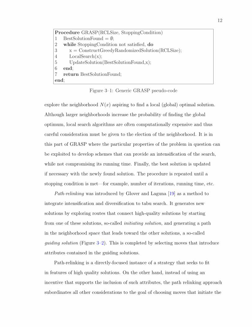
Each iteration of GRASP consists of two phases: a construction phase in
which we seek to obtain a feasible solution, and a local search phase that attempts
to improve the solution. Figure 3–1 shows the pseudo-code of a generic GRASP
algorithm.
During the construction phase, we iteratively build a solution by randomly
selecting objects from a restricted candidate list (RCL). At each step, we form the
RCL choosing those objects with the highest measure of attractiveness, we select a
random object from the RCL, and adapt the greedy function to reflect the addition
to the solution. Figure 3–4 shows the construction phase for our implementation.
The size of the list is typically restricted in one of two ways: by quality,
when we choose the elements based on a threshold on the greedy function, or by
cardinality. In the literature, they are often referred to as α and β, respectively.
The size of the RCL controls the degree of greediness and randomness of the
construction phase. A null RCL—i.e., of size 1—results in a purely greedy solution
whereas a RCL size equal to the size of the problem yields a purely random
solution.
After a solution is constructed, we attempt to improve it by performing a
local search in an appropriately defined neighborhood. Given a solution x, we
11
12
Procedure GRASP(RCLSize, StoppingCondition)1 BestSolutionFound = ∅;2 while StoppingCondition not satisfied, do3 x = ConstructGreedyRandomizedSolution(RCLSize);4 LocalSearch(x);5 UpdateSolution(BestSolutionFound,x);6 end;7 return BestSolutionFound;end;
Figure 3–1: Generic GRASP pseudo-code
explore the neighborhood N(x) aspiring to find a local (global) optimal solution.
Although larger neighborhoods increase the probability of finding the global
optimum, local search algorithms are often computationally expensive and thus
careful consideration must be given to the election of the neighborhood. It is in
this part of GRASP where the particular properties of the problem in question can
be exploited to develop schemes that can provide an intensification of the search,
while not compromising its running time. Finally, the best solution is updated
if necessary with the newly found solution. The procedure is repeated until a
stopping condition is met—for example, number of iterations, running time, etc.
Path-relinking was introduced by Glover and Laguna [19] as a method to
integrate intensification and diversification to tabu search. It generates new
solutions by exploring routes that connect high-quality solutions by starting
from one of these solutions, so-called initiating solution, and generating a path
in the neighborhood space that leads toward the other solutions, a so-called
guiding solution (Figure 3–2). This is completed by selecting moves that introduce
attributes contained in the guiding solutions.
Path-relinking is a directly-focused instance of a strategy that seeks to fit
in features of high quality solutions. On the other hand, instead of using an
incentive that supports the inclusion of such attributes, the path relinking approach
subordinates all other considerations to the goal of choosing moves that initiate the
13
x
Obj
ecti
ve F
unct
ion
Val
ue
Solution
gN(p)
p
Figure 3–2: Visualization of a path-relinking procedure. Given the initial solutionx and the guiding solution g, we iteratively explore the trajectory linking thesesolutions, checking for any improvements on the way.
attributes of the guiding solutions, in order to generate a good attribute composition
in the current solution. The composition at each step is determined by choosing the
best move, using customary choice criteria, from the restricted set of moves that
incorporate a maximum number of the attributes of guiding solutions.
Laguna and Martı [20] were the first to combine GRASP with a path-relinking
procedure, essentially adding memory to a procedure that would otherwise be a
multi-start algorithm.
3.2 Proposed Algorithm
In this section we propose a new heuristic that integrates GRASP with path-
relinking for the linear ordering problem. Figure 3–3 shows the pseudo-code for the
implementation.
The measure of attractiveness for each object i consists of the difference
between its row and column sums, given by
di =n∑
j=1
(eij − eji), i = 1, 2, . . . , n. (3.1)
14
Procedure GRASP(β, ρ, MaxIteration)01 BestSolutionFound = ∅;02 EliteList = ∅;03 nNonImprovingIt = 0;04 for k = 1,2,...,MaxIteration05 x = ConstructGreedyRandomizedSolution(β);06 LocalSearch(x);07 if x is better than worse solution in EliteList08 DoPathRelinking(EliteList,x);09 nNonImprovingIt = 0;10 else if nNonImprovingIt > γ11 ExpandEliteList(EliteList,ρ);12 DoPathRelinking(EliteList,x);13 nNonImprovingIt = 0;14 else nNonImprovingIt = nNonImprovingIt + 1;13 UpdateSolution(BestSolutionFound,x);14 end;15 return BestSolutionFound;end;
Figure 3–3: GRASP pseudo-code
In the context of the input-output tables, Equation 3.1 represents the net flow
of a sector. In earlier experimentations with a GRASP algorithm, we compared
the use of Equation 3.1 with the ratios as defined in Equation 2.9. Although we
have not observed significant differences in the quality of the solutions, adapting
the greedy function when ratios are used is computationally more expensive. The
use of Equation 2.9 demands O(n2) time to update the greedy function whereas
Equation 3.1 requires O(n) time.
Linear ordering problems usually have many alternative solutions—optimal
and suboptimal—with the same objective function value. Therefore, it may occur
at some point in the algorithm that the elite list becomes mostly populated by
alternative solutions. Furthermore, it is increasingly difficult to enter a path-
relinking as the best solution found approaches the optimal. We attempt to avoid
such situations by expanding the size of the elite list and forcing a path-relinking
procedure after a certain number of non-improving iterations. If an improvement is
15
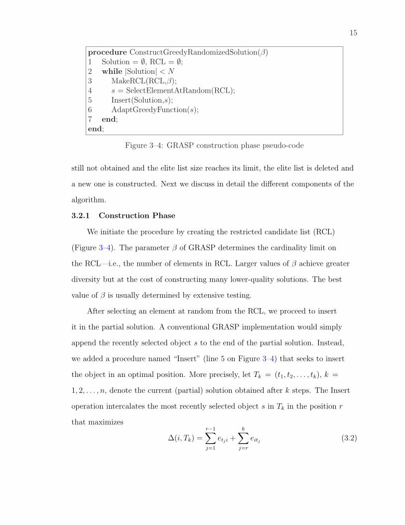
procedure ConstructGreedyRandomizedSolution(β)1 Solution = ∅, RCL = ∅;2 while |Solution| < N3 MakeRCL(RCL,β);4 s = SelectElementAtRandom(RCL);5 Insert(Solution,s);6 AdaptGreedyFunction(s);7 end;end;
Figure 3–4: GRASP construction phase pseudo-code
still not obtained and the elite list size reaches its limit, the elite list is deleted and
a new one is constructed. Next we discuss in detail the different components of the
algorithm.
3.2.1 Construction Phase
We initiate the procedure by creating the restricted candidate list (RCL)
(Figure 3–4). The parameter β of GRASP determines the cardinality limit on
the RCL—i.e., the number of elements in RCL. Larger values of β achieve greater
diversity but at the cost of constructing many lower-quality solutions. The best
value of β is usually determined by extensive testing.
After selecting an element at random from the RCL, we proceed to insert
it in the partial solution. A conventional GRASP implementation would simply
append the recently selected object s to the end of the partial solution. Instead,
we added a procedure named “Insert” (line 5 on Figure 3–4) that seeks to insert
the object in an optimal position. More precisely, let Tk = (t1, t2, . . . , tk), k =
1, 2, . . . , n, denote the current (partial) solution obtained after k steps. The Insert
operation intercalates the most recently selected object s in Tk in the position r
that maximizes
∆(i, Tk) =r−1∑j=1
etji +k∑
j=r
eitj (3.2)
16
breaking ties arbitrarily. First introduced by Chanas and Kobylanski [14] as part of
their heuristic, it can be considered as a very efficient local search procedure in a
relatively small neighborhood. In fact, it can be implemented in O(k).
A step of the contruction phase finalizes with the task of adapting the greedy
function. The row and column corresponding to the object s are removed from the
matrix, and the attractiveness of the objects (Equation 3.1) is updated. We set
ds = −M , where M is a large positive value, and re-sort the top n− k objects that
have yet to be selected. The procedure continues until a solution is constructed.
The overall complexity of the construction phase is O(n2).
3.2.2 Local Search
We used a 2-exchange neighborhood for our local search. Given a solution
π, its 2-exchange neighborhood N(π) consists of all the solutions obtained by
permuting the position of two objects in the ordering—i.e., if π = (3, 1, 2), then
N(π) = {(1, 3, 2), (2, 1, 3), (3, 2, 1)}. Clearly, for a problem of size n, |N(π)| =(
n2
).
Consider a solution π and two objects π(i) and π(j) located in positions i and j
respectively. For simplicity assume that i < j. The change in the objective function
for an exchange of objects π(i) and π(j) is
∆Z(π, i, j) = −e′π(i)π(j) −j−1∑
k=i+1
(e′π(i)π(k) + e′π(k)π(j)) (3.3)
where e′ij = eij − eji. At completion, the local search would have exchanged
the pair of objects that maximizes Equation 3.3. The procedure of exploring the
neighborhood and performing the exchange can be implemented in O(n2).
3.2.3 Path Relinking
The solution provided by the local search procedure is used as the initial
solution for the path-relinking. We randomly select a solution from the elite list as
the guiding solution, determining the trajectory to be followed by the procedure.
17
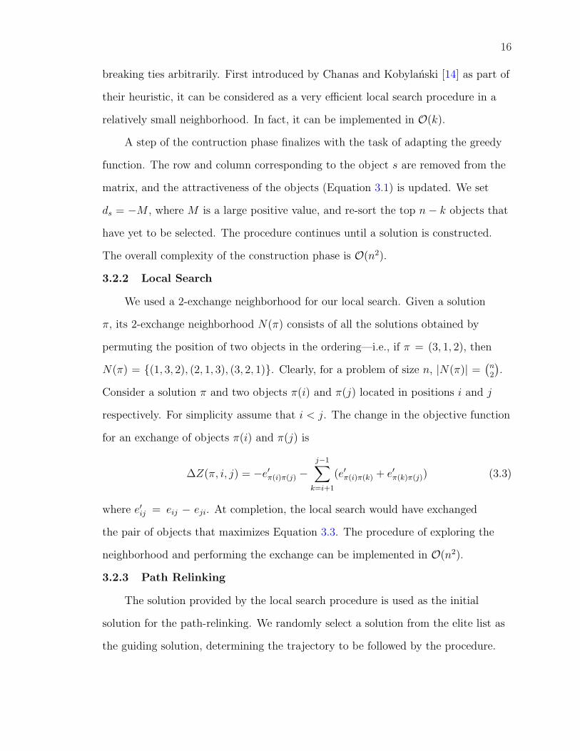
procedure DoPathRelinking(EliteList,x)1 TempSolution = ∅;2 g = SelectSolutionAtRandom(EliteList);3 while x 6= g do4 TempSolution = MakeNextMove(x, g);5 LocalSearch(TempSolution);6 if TempSolution is better than x or g then7 EliteList = EliteList ∪ TempSolution;8 end;9 AdjustEliteList(EliteList,ρ);end;
Figure 3–5: GRASP path-relinking pseudo-code
Figure 3–5 shows the pseudo-code for the path relinking procedure. The parameter
ρ determines the size of the elite list as a fraction of the problem size.
With the trajectory defined by the two end solutions, we proceed to perform
a series of moves that will transform the initial solution into the guiding solution.
In each iteration the algorithm performs a single move, thus creating a sequence
of intermediate solutions (Figure 3–2). To add intensification to the process, we
search the 2-exchange neighborhood of the intermediate solutions. The solutions
obtained in this manner are added to the elite list if they are better than either the
initial or the guiding solutions.
It should be noted that the search on the 2-exchange neighborhood may yield
a previously examined solution in the path. However, this is not of concern in our
implementation since we do not use the local minima during the procedure.
The moving process terminates when the algorithm reaches the guiding
solution. At this point, the elite list size could have grown considerably due to the
added solutions. The procedure “AdjustEliteList” will discard the worst solutions,
keeping the best ρn. The list is kept sorted at all times and therefore no sorting is
needed. The complexity of the path-relinking is O(n3).
CHAPTER 4COMPUTATIONAL RESULTS
Here we discuss the computational results we obtained when applying our
algorithm to two sets of problems:
• LOLIB. These are real-world instances of linear ordering problems that arepublicly available on the internet [21]. They consist of 49 input-output tablesfor some European countries, with sizes up to 60 objects.
• Mitchell. This is a set of 30 randomly-generated instances by Mitchell [10],with sizes ranging from 100 to 250 objects. Three different percentages ofzero entries were used: 0, 10, and 20%, denoted by the last digit on theproblem name. The generator as well as the instances are available at theauthor’s web site [22].
The optimal values for all instances are known. The generated instances
are similar to those from LOLIB except for the numerical range of the entries—
considerably larger for the latter. Despite attempts to replicate the characteristics
of real-world instances such as those found in LOLIB, Mitchell’s test set is
significantly harder to solve. All previous work on the linear ordering problem
that included computational results predates the Mitchell instances, hence featuring
only the LOLIB problems.
The algorithm was written in C++ and executed on a Pentium 4, 2.7 GHz,
with 512 MB of memory. Empirically, we determined β = 0.25 and ρ = 0.35 as
the best values for the parameters (e.g., for a problem of size n, the size of the
RCL and the elite list are at most 0.25n and 0.35n respectively). The algorithm
was executed five times for each problem instance, with a limit of 5000 GRASP
iterations on its running time. We report the running time, number of iterations,
18
19
and the gap between the best solution and the optimal solution. All times are
reported in seconds and gaps as percentages.
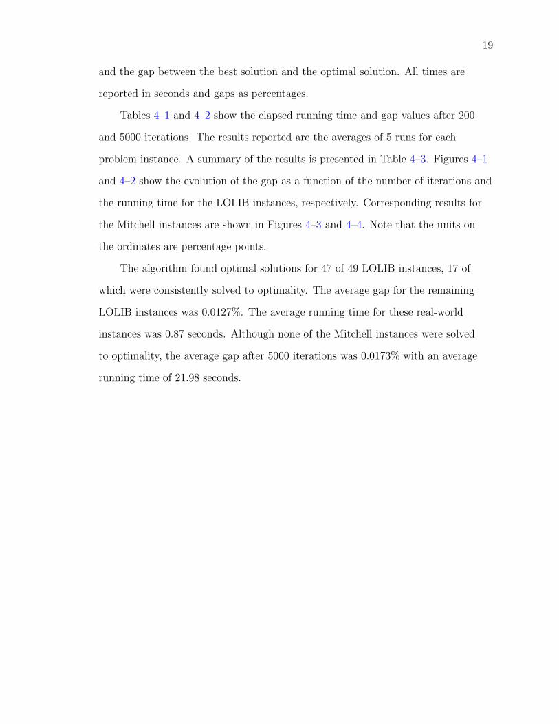
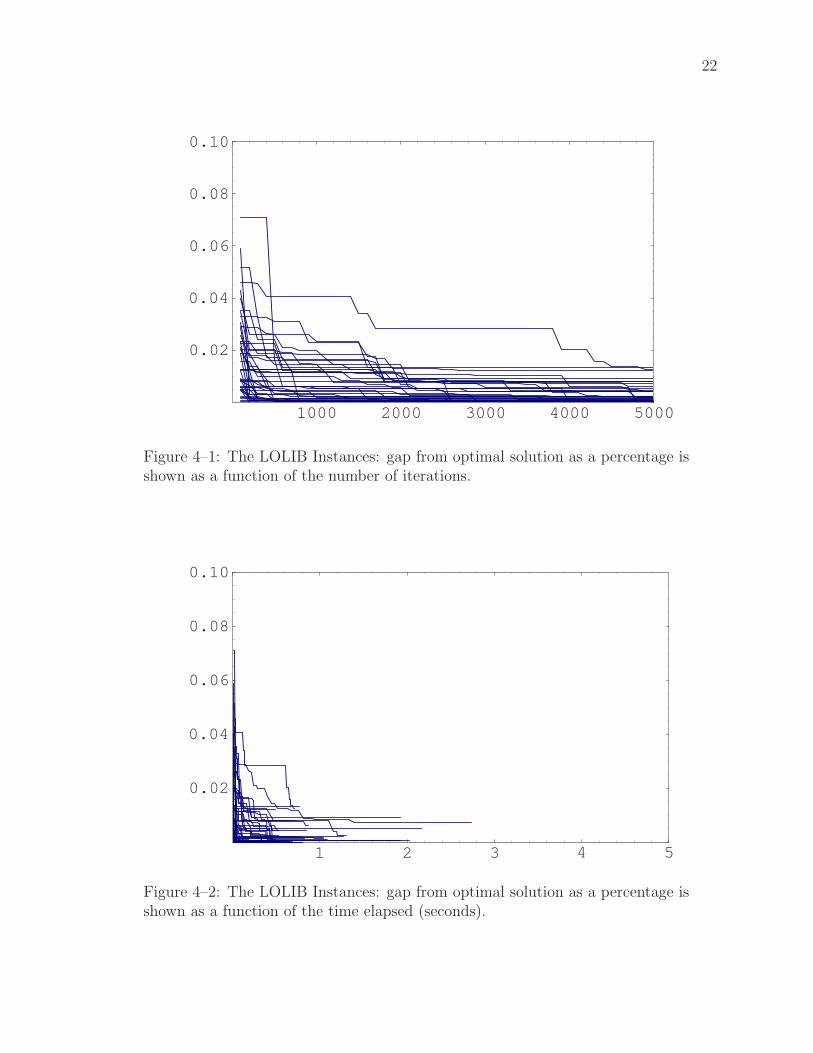
Tables 4–1 and 4–2 show the elapsed running time and gap values after 200
and 5000 iterations. The results reported are the averages of 5 runs for each
problem instance. A summary of the results is presented in Table 4–3. Figures 4–1
and 4–2 show the evolution of the gap as a function of the number of iterations and
the running time for the LOLIB instances, respectively. Corresponding results for
the Mitchell instances are shown in Figures 4–3 and 4–4. Note that the units on
the ordinates are percentage points.
The algorithm found optimal solutions for 47 of 49 LOLIB instances, 17 of
which were consistently solved to optimality. The average gap for the remaining
LOLIB instances was 0.0127%. The average running time for these real-world
instances was 0.87 seconds. Although none of the Mitchell instances were solved
to optimality, the average gap after 5000 iterations was 0.0173% with an average
running time of 21.98 seconds.
20
Table 4–1: Results for the LOLIB Instances after 200 and 5000 iterations.
Instance Size 200 Iterations 5000 IterationsGap(%) Time (s) Gap(%) Time (s)
Figure 4–1: The LOLIB Instances: gap from optimal solution as a percentage isshown as a function of the number of iterations.
1 2 3 4 5
0.02
0.04
0.06
0.08
0.10
Figure 4–2: The LOLIB Instances: gap from optimal solution as a percentage isshown as a function of the time elapsed (seconds).
23
1000 2000 3000 4000 5000
0.02
0.04
0.06
0.08
0.10
Figure 4–3: Mitchell Instances: gap from optimal solution as a percentage is shownas a function of the number of iterations.
10 20 30 40 50 60
0.02
0.04
0.06
0.08
0.10
Figure 4–4: Mitchell Instances: gap from optimal solution as a percentage is shownas a function of the time elapsed (seconds).
CHAPTER 5CONCLUDING REMARKS
Our study implemented a new heuristic algorithm for the linear ordering
problem, inspired by its application to the triangulation of input-output tables
in economics. The algorithm is based on a greedy randomized adaptive search
procedure (GRASP) with the addition of a path-relinking phase to further intensify
the search.
The algorithm was tested on two sets of problems, exhibiting a remarkably
robust performance as shown in Table 4–3. For all instances we obtained optimality
gaps of less than 0.05% within 200 iterations and times ranging from 0.02 to
2.40 seconds on the average. We found optimal solutions for most of the LOLIB
instances. No optimal solutions were obtained for the Mitchell instances, however,
the average gap at termination for this set was 0.0173%. The results confirm the
benefit of embedding GRASP with a path-relinking procedure.
Researchers in economics often use simulations in which many triangulation
problems need to be solved in limited time. The efficiency and high-quality
performance of our algorithm makes it a superior candidate for such application.
Furthermore, since the algorithm is based upon the modelling of the triangulation
problem as a linear ordering problem (LOP), it can be used for any application
that accepts an LOP formulation such as those mentioned in Section 2.1.
We believe that further research is required for analyzing the relation of the
LOP with other known problems. In particular, could the LOP be thought of as a
travelling salesman problem where, in addition to the distances between locations,
we have priorities assigned each of these? Could we use the extensive research done
24
25
in the TSP as a basis for the LOP? Answers to these and other related questions
will be pursued in future research.
REFERENCES
[1] Wassily Leontief, Input-Output Economics, Oxford University Press, NewYork, USA, 1986.
[2] George B. Dantzig, “Linear programming,” Operations Research, vol. 50, no.1, pp. 42–47, January 2002.
[3] Gerhard Reinelt, The linear ordering problem: algorithms and applications,Number 8 in Research and Exposition in Mathematics. Heldermann Verlag,Berlin, Germany, 1985.
[4] Michael Junger, Polyhedral Combinatorics and the Acyclic SubdigraphProblem, Number 7 in Research and Exposition in Mathematics. HeldermannVerlag, Berlin, 1985.
[5] Michael R. Garey and David S. Johnson, Computers and Intractability: AGuide to the Theory of NP-Completeness, W.H. Freeman and Co., New York,USA, 1979.
[6] R.E. Burkard, E. Cela, P.M. Pardalos, and L.S. Pitsoulis, “The quadraticassignment problem,” in Handbook of Combinatorial Optimization, P.M.Pardalos and D.-Z. Du, Eds., pp. 241–338. Kluwer Academic Publishers, 1998.
[7] Martin Grotschel, Michael Junger, and Gerhard Reinelt, “A cutting planealgorithm for the linear ordering problem,” Operations Research, vol. 2, no. 6,pp. 1195–1220, 1984.
[8] G. Bolotashvili, M. Kovalev, and E. Girlich, “New facets of the linear orderingpolytope,” SIAM Journal on Discrete Mathematics, vol. 12, no. 3, pp.326–336, 1999.
[9] Thomas Christof, Low-Dimensional 0/1-Polytopes and Branch-and-Cut inCombinatorial Optimization, Ph.D. dissertation, University of Heidelberg,Heidelberg, Germany, 1997.
[10] John E. Mitchell, “Computational experience with an interior point cuttingplane algorithm,” Tech. Rep., Mathematical Sciences, Rensellaer PolytechnicIntitute, Troy, NY 12180-3590, USA, 1997.
[11] John E. Mitchell and Brian Borchers, “Solving linear ordering problemswith a combined interior point/simplex cutting plane algorithm,” in HighPerformance Optimization, H. Frenk et al., Ed., chapter 14, pp. 345–366.Kluwer Academic Publishers, Dordrecht, The Netherlands, 2000.
26
27
[12] Rafael Martı, “Multi-start methods,” in Handbook of Metaheuristics, FredGlover and Gary A. Kochenberger, Eds., International Series in OperationsResearch & Management Sciences, chapter 12, pp. 355–368. Kluwer AcademicPublishers, Dordrecht, The Netherlands, 2003.
[13] Hollis B. Chenery and Tsunehiko Watanabe, “International comparisons of thestructure of production,” Econometrica, vol. 26, no. 4, pp. 487–521, October1958.
[14] Stefan Chanas and PrzemysÃlaw Kobylanski, “A new heuristic algorithmsolving the linear ordering problem,” Computational Optimization andApplications, vol. 6, pp. 191–205, 1996.
[15] Manuel Laguna, Rafael Martı, and Vicente Campos, “Intensification anddiversification with elite tabu search solutions for the linear ordering problem,”Computers & Operations Research, vol. 26, pp. 1217–1230, 1999.
[16] Vicente Campos, Fred Glover, Manuel Laguna, and Rafael Martı, “Anexperimental evaluation of a scatter search for the linear ordering problem,”Journal of Global Optimization, vol. 21, no. 4, pp. 397–414, December 2001.
[17] Thomas A. Feo and Mauricio G.C. Resende, “Greedy randomized adaptivesearch procedures,” Journal of Global Optimization, vol. 2, pp. 1–27, 1995.
[18] Paola Festa, Mauricio G.C. Resende, and Geraldo Veiga, “Annotatedbibliography of GRASP,” AT&T Research Labs, Jan. 2004,http://www.research.att.com/∼mgcr/grasp/annotated.
[19] Fred Glover and Manuel Laguna, Tabu Search, Kluwer Academic Publishers,Boston, USA, 1997.
[20] Manuel Laguna and Rafael Martı, “GRASP and path relinking for 2-layerstraight line crossing minimization,” INFORMS Journal on Computing, vol.11, no. 1, pp. 44–52, 1998.
[21] Gerhard Reinelt, “Linear ordering library (LOLIB),” University of Heidelberg,Dec. 2002,http://www.iwr.uni-heidelberg.de/groups/comopt/software/LOLIB/.
[22] John E. Mitchell, “Generating linear ordering problems,” Rensellaer Polytech-nic Intitute, Dec. 2002, http://www.rpi.edu/∼mitchj/generators/linord.
BIOGRAPHICAL SKETCH
Bruno H. Chiarini was born on December 21, 1974, in Buenos Aires,
Argentina. In 1996 he was admitted to the Instituto Tecnologico de Buenos Aires
(ITBA). He transferred to the University of Florida in January 2001, where he was
awarded a Bachelor of Science degree in Industrial and Systems Engineering in
August 2002. He then pursued graduate studies at the same institution, obtaining
a Master of Science degree in Industrial and Systems Engineering in May 2004.