New Approach to the Modeling of Complex Multibody...

1

amlmdvtecdw�shcahmsm

msgrota

JrD

J

Downlo

Aaron SchutteDepartment of Aerospace and Mechanical

Engineering,University of Southern California,

Los Angeles, CA 90089-1453e-mail: [email protected]

Firdaus UdwadiaProfessor

Departments of Aerospace and MechanicalEngineering, Civil Engineering, Mathematics,

Systems Architecture Engineering, andInformation and Operations Management,

University of Southern California,430K Olin Hall,

Los Angeles, CA 90089-1453e-mail: [email protected]

New Approach to the Modeling ofComplex Multibody DynamicalSystemsIn this paper, a general method for modeling complex multibody systems is presented.The method utilizes recent results in analytical dynamics adapted to general complexmultibody systems. The term complex is employed to denote those multibody systemswhose equations of motion are highly nonlinear, nonautonomous, and possibly yieldmotions at multiple time and distance scales. These types of problems can easily becomedifficult to analyze because of the complexity of the equations of motion, which may growrapidly as the number of component bodies in the multibody system increases. The ap-proach considered herein simplifies the effort required in modeling general multibodysystems by explicitly developing closed form expressions in terms of any desirable num-ber of generalized coordinates that may appropriately describe the configuration of themultibody system. Furthermore, the approach is simple in implementation because itposes no restrictions on the total number and nature of modeling constraints used toconstruct the equations of motion of the multibody system. Conceptually, the methodrelies on a simple three-step procedure. It utilizes the Udwadia–Phohomsiri equation,which describes the explicit equations of motion for constrained mechanical systems withsingular mass matrices. The simplicity of the method and its accuracy is illustrated bymodeling a multibody spacecraft system. �DOI: 10.1115/1.4002329�

Keywords: multibody dynamics, singular mass matrix, general constrained systems, mul-tiscale dynamical systems, use of more generalized coordinates than minimum

IntroductionThe motion of a multibody system is generally highly nonlinear

nd often complex. Formulating equations of motion for generalultibody systems can be a nontrivial task, and in many formu-

ations the equations of motion are restricted to case specificultibody problems. Recently, a fundamental result in analytical

ynamics obtained by Udwadia and Kalaba �1–4� led to a newiew in the theory of constrained motion, which is intimately tiedo multibody dynamics. They obtain explicitly a general set ofquations of motion for holonomically and nonholonomicallyonstrained mechanical systems in terms of the generalized coor-inates that describe their configuration. In a further advance, Ud-adia and Phohomsiri �5� obtained an explicit equation of motion

Udwadia–Phohomsiri �UP� equation� for constrained mechanicalystems with singular mass matrices. While it may not be obviousow singular mass matrices might arise when describing the un-onstrained motion of a mechanical system, we note that they dorise when modeling multibody systems. The approach proposederein permits the deft handling of systems with singular massatrices, thereby permitting the description of complex multibody

ystems through the use of a larger number of coordinates than theinimum required.The value of a method that is used to obtain the equations ofotion for a complex multibody system should be measured by its

implicity and the amount of effort required when deriving theoverning equations of the correctly modeled multibody system aseasoned in surveys by Kane �6� and Schiehlen �7�. The method-logy proposed herein aims at this goal. It significantly simplifieshe effort in obtaining the equations of motion of such systems byllowing the modeler to apply the following: �1� use of more than

Contributed by the Applied Mechanics Division of ASME for publication in theOURNAL OF APPLIED MECHANICS. Manuscript received July 28, 2009; final manuscripteceived July 23, 2010; accepted manuscript posted August 9, 2010; published online
ecember 20, 2010. Assoc. Editor: Wei-Chau Xie.
ournal of Applied Mechanics Copyright © 20

aded 01 Feb 2011 to 130.221.224.7. Redistribution subject to ASME

the minimum number of coordinates to describe the motion ofeach subsystem of a complex multibody system, �2� inclusion ofany, and all, constraints that can be discerned in the description ofthe various connections between the subsystems used to model thecomplex system without worrying about which constraints may befunctionally dependent, and �3� use of a formulation that seam-lessly includes positive semidefinite and/or positive definite massmatrices.

In many popular multibody modeling methods available todate, the equations of motion are generated using recursive meth-ods. Most recursive methods are employed by casting a multibodysystem into a tree topology wherein each individual body in themultibody system is attached to one or more of the other bodiesthat comprise the whole system. The bodies are attached to oneanother at joints located at arbitrarily given fixed points on eachindividual body. The coordinates in these systems are taken rela-tive to the so-called joint coordinates �relative displacements androtations between component bodies� so that the equations of mo-tion are obtained in terms of the independent degrees of freedom.These approaches attempt to provide a reduction in the total num-ber of coordinates with the primary goal of increasing computa-tional performance, a topic on which considerable research inter-est seems to have been focused �e.g., Refs. �8–10��. While it istrue that a reduction in the number of coordinates can ideallyincrease computational performance, it often does so at the cost ofincreased difficulty in arriving at the equations of motion. In ad-dition, these approaches force the modeling to be conceptualizedwithin a predefined modeling structure, one that requires the con-struction of the multibody system to take place along lineal linesof thought that more or less reflect the underlying paradigmatictree-structure. This aspect could be a source of considerable in-convenience, especially when constraints need to be altered, be-cause this might at times require a complete remodeling of themultibody system. Also, as pointed out by several researchers,applying general constraint equations or forcing functions can be-
come problematic in some situations for recursive methods �11�.
MARCH 2011, Vol. 78 / 021018-111 by ASME

license or copyright; see http://www.asme.org/terms/Terms_Use.cfm

oe�twnccsnasnep

mwodcuetaiepbmtwmdt

2

twwcs

ectaac

CNswc=a�o

0

Downlo

Other approaches for generating the governing equations relyn the computation of Lagrange multipliers �12,13�, or by thelimination of Lagrange multipliers via null space methods14,15�. The so-called null space method relies on the computa-ion of an orthogonal complement of the constraint matrix inhich the constraints are required to be linear in the velocities andonredundant. These methods are difficult to apply to generalomplex multibody systems and they fail in situations where theonstraints are functionally dependent. While holonomic con-traints are often easy to spot when they are not independent,onholonomic constraints take the form of differential equationsnd in highly complex systems, which may have many such con-traints, ensuring that they are all independent could become aontrivial job. This is because two differential equations, thoughquivalent, can take on very different-looking forms when multi-lied by various multiplying factors.

In the following, a new and simple approach of systematicallyodeling a complex system of N rigid bodies is developedherein we posit no predefined modeling structure on the devel-pment of the equations of motion, and in implementation theesired computational performance may not be realized due to theomputational overhead of the recursion. The term complex issed in this paper to denote those systems that are highly nonlin-ar, possibly nonautonomous, and that may yield motions at mul-iple time and distance scales. One of the salient advantages of ourpproach is its conceptual clarity. The modeling methodology andts formulation are simple, and the effort required to obtain thequations of motion is minimal, thereby allowing a uniform, im-roved, and widely applicable route for modeling complex multi-ody systems. The method exploits the appearance of singularass matrices in Lagrangian mechanics by utilizing the UP equa-

ion, thereby overcoming a difficulty that is not easily handledith current methods �5�. In an example, we show its use for theodeling of a realistic multiscale, multibody spacecraft system to

emonstrate the simplicity of the approach, its ease of implemen-ation, and its numerical accuracy.

Modeling Complex Multibody SystemsA general formulation is developed in this section to describe

he dynamics of multiple interconnected rigid bodies. Beginningith the concepts of generalized coordinates and kinetic energy,e describe how to obtain the explicit equations of motion for

omplex multibody systems using a simple straightforward three-tep procedure. Conceptually, these three steps are the following:

�i� description of the so-called unconstrained system of equa-tions

�ii� description of the constraints required to model the givenmultibody system

�iii� description of the constrained multibody system using theprevious two descriptions

In what follows, we develop each of these steps pointing out thease and efficacy with which the equations of motion for generalomplex multibody dynamical systems can be obtained. In ordero provide an explicit framework for our modeling methodologynd establish our notation, we begin by considering the motion ofrigid body wherein we permit the use of an arbitrary number of

oordinates to describe its motion.

2.1 Generalized Coordinates and Kinetic Energy of aomponent Body in a Multibody System Using an Arbitraryumber of Coordinates to Describe Its Motion. Consider first a

ingle rigid body that is a component of the multibody system thate desire to model. Let its mass be m and let the position to its

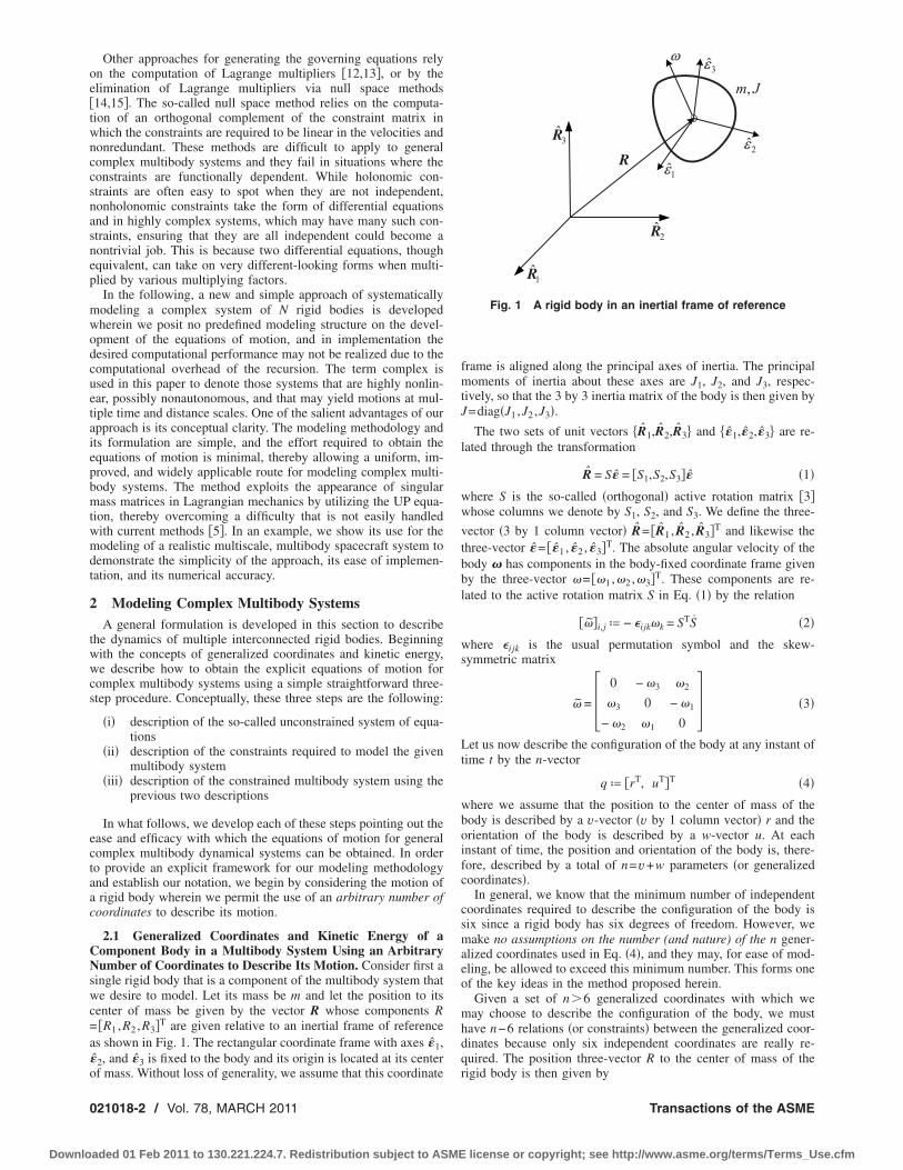
enter of mass be given by the vector R whose components R�R1 ,R2 ,R3�T are given relative to an inertial frame of references shown in Fig. 1. The rectangular coordinate frame with axes �1,

ˆ 2, and �3 is fixed to the body and its origin is located at its center
f mass. Without loss of generality, we assume that this coordinate
21018-2 / Vol. 78, MARCH 2011


frame is aligned along the principal axes of inertia. The principalmoments of inertia about these axes are J1, J2, and J3, respec-tively, so that the 3 by 3 inertia matrix of the body is then given byJ=diag�J1 ,J2 ,J3�.

The two sets of unit vectors �R1,R2,R3� and ��1,�2,�3� are re-lated through the transformation

R = S� = �S1,S2,S3�� 1�

where S is the so-called �orthogonal� active rotation matrix �3�whose columns we denote by S1, S2, and S3. We define the three-

vector �3 by 1 column vector� R= �R1 , R2 , R3�T and likewise thethree-vector �= ��1 , �2 , �3�T. The absolute angular velocity of thebody � has components in the body-fixed coordinate frame givenby the three-vector �= ��1 ,�2 ,�3�T. These components are re-lated to the active rotation matrix S in Eq. �1� by the relation

��i,j ª − �ijk�k = STS �2�

where �ijk is the usual permutation symbol and the skew-symmetric matrix

� = � 0 − �3 �2

�3 0 − �1

− �2 �1 0� �3�

Let us now describe the configuration of the body at any instant oftime t by the n-vector

q ª �rT, uT�T �4�

where we assume that the position to the center of mass of thebody is described by a v-vector �v by 1 column vector� r and theorientation of the body is described by a w-vector u. At eachinstant of time, the position and orientation of the body is, there-fore, described by a total of n=v+w parameters �or generalizedcoordinates�.

In general, we know that the minimum number of independentcoordinates required to describe the configuration of the body issix since a rigid body has six degrees of freedom. However, wemake no assumptions on the number (and nature) of the n gener-alized coordinates used in Eq. �4�, and they may, for ease of mod-eling, be allowed to exceed this minimum number. This forms oneof the key ideas in the method proposed herein.

Given a set of n�6 generalized coordinates with which wemay choose to describe the configuration of the body, we musthave n−6 relations �or constraints� between the generalized coor-dinates because only six independent coordinates are really re-quired. The position three-vector R to the center of mass of the

ω

Jm,

1R

2R

3R

R1ε

2ε

3ε

Fig. 1 A rigid body in an inertial frame of reference

rigid body is then given by

Transactions of the ASME


s

wm

Uvt

w

w

atptc

asropc

cpiuct

wf

atwos

uoWtbp

=e

J

Downlo

R = R�r1,r2, . . . ,rv� ª R�r� �5�

o that R is then simply

R =�R

�rr ª G�r�r �6�

here G is a 3 by v matrix. Similarly, each element of the rotationatrix S is a function of the elements of the w-vector u so that1

S = S�u1,u2, . . . ,uw� ª S�u� �7�sing Eq. �2�, we can then express the components of the angularelocity vector � in the body-fixed coordinate frame so that thehree-vector � can be expressed as

� = H�u�u �8�

here H�u� is a 3 by w matrix.By Eqs. �6� and �8�, the total kinetic energy of the body is

T =1

2mR · R +

1

2�TJ� =

1

2mrTGTGr +

1

2uTHTJHu =

1

2qTM�q�q

�9�

here the n by n block-diagonal matrix

M�q� = diag�mGTG, HTJH� �10�

nd the matrices G and H are functions of q. It should be notedhat the matrix M may not be positive definite, in general, but onlyositive semidefinite. This comes about because we have modeledhe rigid body with an arbitrary number �n�6� of generalizedoordinates.

For example, suppose we choose the generalized coordinate us the four-vector of �unit norm� quarternions, a coordinate welluited for the parameterization of rigid body rotations �16�. Theesultant matrix H in Eq. �8� would then become a 3 by 4 matrixf rank three. This causes the matrix HTJH in Eq. �10� to becomeositive semidefinite. Consequently, the matrix M will also be-ome positive semidefinite �singular�.

2.2 Description of the Unconstrained System and the Un-onstrained Equations of Motion. The next key idea in our ap-roach is to assume that the n generalized coordinates are allndependent of each other. We, thus, apply Lagrange’s equationnder the assumption, that all the components of the generalizedoordinate n-vector q are independent. Thus, for any one bodyhat comprises the multibody system, we have

d

dt �T

� qk −

�T

�qk= Qk, k = 1,2, . . . ,n �11�

here Q is an n-vector that contains the generalized “given”orces and torques �part of which may be derived from a potential�cting on the body. The n-vector Q= ��T , �T�T is composed ofhe generalized force v-vector � and the generalized torque-vector �. Equation �11� will yield, in general, a set of n second-rder nonlinear, nonautonomous differential equations, which areimply expressed in the form

Mq = Q �12�

The n-vector Q on the right hand side of Eq. �12� contains, as

sual, the generalized “impressed” force-torque vector Q andther additional terms generated by applying Lagrange’s equation.e note that because of the flexibility provided in the choice of

he number �and nature� of the coordinates in the n-vector q andecause of our assumption that all the components of q are inde-endent, the equations of motion in Eq. �12� are obtained with

1In general, we could take R=R�r1 ,r2 , . . . ,rv , t�ªR�r , t� in Eq. �5� and SS�u1 ,u2 , . . . ,uw , t�ªS�u , t� in Eq. �7�, but for the sake of simplicity and clarity of
xposition we do not explicitly include the time t in these equations.
ournal of Applied Mechanics


considerable ease. Also, the generalized force-torque vector Q isnear-trivial to obtain since the virtual displacements of all thecomponents of q are assumed independent of each other. How-ever, since the generalized coordinates q may not in actuality beindependent of one another as we have assumed, the matrix Mgiven by Eq. �10� is, in general, only positive semidefinite.

Now that we have described the equations of motion for asingle component body of a multibody system in terms of thegeneralized coordinates used to describe its position and orienta-tion, we can proceed in a similar manner to obtain the equationsof motion for each of the N bodies that comprise the entire multi-body system. Let body “i” of the multibody system have mass mi

and an inertia matrix Ji. We shall denote quantities relevant tobody i by the superscript i. The position and orientation of body iis then described by the ni-component column vector of general-ized coordinates qi as described in Eq. �4�. Thus, we have a totalof

K = �i=1

N

ni �13�

generalized coordinates that specify the configuration of the multi-body system, and we assemble these generalized coordinates intothe K-vector q= ��q1�T , �q2�T , . . . , �qN�T�T. The ni-vectors Qi �and

Qi� are now, in general, functions of the K-vectors q and q thatdescribe the configuration of the multibody system and its gener-alized velocity.

Under the assumption that the generalized coordinates describ-ing the configuration of each rigid body �the components of thevector qi� are all independent of one another and that the coordi-nates qi and qj for all i� j, i , j� �1,N� are independent of oneanother, we next assemble the Lagrange equations for the entiremultibody system as

Mq ª �M1 0 ¯ 0

0 M2¯ 0

] ] � ]

0 0 ¯ MN��

q1

q2

]

qN� = �

Q1

Q2

]

QN�ª Q �14�

where the K by K block-diagonal matrix M is, in general, positivesemidefinite.

We refer to these equations as “unconstrained” since they havebeen arrived at under the assumption that all the components ofthe K-vector q are independent of one another. In other words,when we write the Lagarange equations �Eq. �14��, we assumethat the virtual displacements in each of the coordinates �compo-nents of the K-vector q� are independent of the virtual displace-ments in any of the other coordinates. This forms another keyfeature in our approach. We note that from a numerical implemen-tation standpoint, assembling the so-called unconstrained equa-tions of motion of the system �as done in Eq. �14� by consideringeach individual body that makes up the complex multibody sys-tem� is highly amenable to parallel processing. This makes thepresent approach an excellent candidate for parallelization sincethe equations of motion of each body �or a subgroup of them� canbe independently assembled.

2.3 Description and Specification of the ModelingConstraints. In the second step of our three-step procedure, weimpose all the necessary modeling constraints on the N bodies sothat we appropriately model the complex multibody system. Con-ceptually, we can think of these constraints as forming two cat-egories. The first category of constraints deals with the fact thatwe may have chosen more than the minimum number �i.e., n�6� of generalized coordinates qi that describe the configurationof body i. The second category deals with the fact that since theindividual bodies comprising the multibody system are intercon-

i ˙ i
nected, the components of the vectors q and q may be affected by
MARCH 2011, Vol. 78 / 021018-3


ttos

c

oeqddsss

wtciWat

wE�m�qdamaw

wccbmc�s�pkibbptt

lmtcta�ria

0

Downlo

hose of qj and qj at each instant of time. The second category,hus, includes all those physical interactions described by meansf constraints between bodies i and j that form the multibodyystem. We use the following notation to describe them.

The first category of constraints is dealt with by imposing theoordinate constraints �requirements�

�ki �qi,t� = 0, i = 1,2, . . . ,N, k = 1,2, . . . ,ni − 6 �15�

n Eq. �14�. These g=K−6N constraints reflect the fact that forach body i, the components of the generalized coordinate vectori may not be independent of one another. To “construct” theesired complex multibody system from its component bodies, weefine the physical interactions, or additional modeling con-traints, between each of the bodies that make up the multibodyystem. We include interactions that are governed by the con-traint equations

�k�q,t� = 0, k = 1,2, . . . ,h �16�

�k�q, q,t� = 0, k = 1,2, . . . ,s �17�

hich include holonomic and nonholonomic constraints, respec-ively. Equations �15�–�17� represent all the so-called modelingonstraints, which comprise a total of m=g+h+s relations involv-ng the components of the K-vectors q and q, and the time, t.

hen the consistent set of these m modeling constraint equationsre sufficiently smooth, we can differentiate them with respect toime and obtain the constraint equation

A�q,q,t�q = b�q,q,t� �18�

here A is an m by K matrix and b is an m-vector. Each row ofq. �18� corresponds to one of the m modeling constraints in Eqs.

15�–�17�. The general set of modeling constraints in Eq. �18� thatay be imposed on the “unconstrained” multibody system �Eq.

14�� include constraints that are �1� nonlinear functions of q and˙ , �2� explicitly dependent on time, and �3� functionally depen-ent. The first of these permits nonlinear constraints to be usednd not just those in the so-called Pfaffian form; the second per-its the constraints to yield nonautonomous dynamical systems;

nd the third provides one of the key features of our approachith the following purpose in mind.In a complex multibody system, it can be difficult to determine

hich of the constraints are functionally dependent. This is espe-ially so for systems with nonholonomic constraints since theseonstraints take the form of differential equations as mentionedefore. This often makes it difficult when modeling a complexultibody system to decipher whether a given set �or subset� of

onstraints implies another. In fact, were we to repeat a constraintpossibly in a different form� as part of our set of constraints,tandard methods like the Lagrange multiplier methods will failsee Sec 2.4 below�. This difficulty is directly averted in our ap-roach, thereby greatly easing the modeler’s effort. Thus, anotherey feature of the approach is the facility provided to the modelern placing as many constraints that �s�he can uncover in the multi-ody system without worrying about �a� whether a constraint haseen repeated �possibly in some other form� and/or �b� whether aarticular subset of constraints, in certain regions �or points inime� in the system’s phase space, might imply another constrainthat has also been included in the set.

We note that the methodology proposed herein follows alongogical lines, lines that would be used to mentally construct the

ultibody system. First, one assembles each body that constituteshe multibody system, as was done in Eq. �14�, by using the mostonvenient set of generalized coordinates �with no restriction onhe total number and nature� needed to describe it. Then, onessembles the necessary constraints engendered, as shown in Eq.18� �or alternatively, in Eqs. �15�–�17��. The method does notequire the modeler to undertake the task of identifying all thendependent constraints and weeding out the dependent ones. Any
nd every constraint that can be identified by the modeler can be
21018-4 / Vol. 78, MARCH 2011


included in this set of m constraints.Finally, we present the last step in our three-step modeling pro-

cedure. Using the description of the unconstrained system givenby Eq. �14� along with the description of the modeling constraintsgiven by Eq. �18�, we obtain the explicit equations of motion ofthe complex multibody system.

2.4 Explicit Equations of Motion for Complex MultibodySystems. The presence of the modeling constraints cause gener-alized forces to be exerted on the unconstrained system describedby Eq. �14�. Thus, to accommodate these modeling constraints onthe multibody system, an additional generalized force K-vectorQm must be applied so that the required motion satisfies the con-straints in Eq. �18�. The equation of motion for the complex multi-body system is then simply expressed as

Mq = Q + Qm�q,q,t� �19�

The explicit acceleration for constrained mechanical systemswhen the K by K matrix M is positive semidefinite is obtained byusing the UP equation. Udwadia and Phohomsiri �5� showed thata necessary and sufficient condition for the equation of motion ofsuch a constrained system to yield a unique generalized accelera-tion at each instant of time—a requirement demanded by physicalobservation of mechanical systems—is that the matrix

M = �M AT � �20�

has rank K. The satisfaction of this requirement �the UP rankcondition� can also be viewed as a check to the modeler on thevalidity of the modeling process that has been carried out. This isuseful because it provides in addition to the facility given to themodeler �1� in choosing an arbitrary number of �ni�6� general-ized coordinates to model each rigid body and �2� in placing asmany constraints as can be deciphered in the multibody system, acheck that the modeling has been done in a manner that respectsthe fact that the accelerations in a physical system must beuniquely ascertainable.

Thus, when M0 and the aforementioned rank condition issatisfied, the explicit acceleration of the constrained system isgiven by �5�

q = ��I − A+A�MA

+�Qb ª M+�Q

b �21�

where the � · �+ notation denotes the Moore-Penrose matrix in-verse. If needed, the modeling constraint force, which arises as aresult of the presence of the modeling constraints, can be explic-itly determined by substituting the expression for q from Eq. �21�into Eq. �19� so that

Qm = MM+�Qb − Q �22�

We note that nowhere in this discussion is the notion of aLagrange multiplier invoked. There are several advantages to do-ing this.

�1� The statement of the problem of constrained motion doesnot include the notion of a Lagrange multiplier and, there-fore, quite naturally, nowhere in the final solution of theproblem does it appear.

�2� A Lagrange multiplier is an intermediary notion that wasdeveloped by Lagrange to handle constrained motion; itneeds to be eliminated when one seeks the final solution.

�3� As is clear from the discussion above, recent developmentsin analytical dynamics point to the fact that the equations ofconstrained motion can be obtained explicitly and directlywithout the use of this intermediary notion �and calculationof the Lagrange multiplier� so that parsimony �Occam’srazor� and simplicity would dictate that it need not be in-
voked.


d�wtmcowtcelocL

etbmreonottmmo

rcntUtior

3

atj�toh

J

Downlo

�4� Finally, the standard Lagrange multiplier formulation of theproblem of constrained motion requires the solution of theaugmented �K+m� by �K+m� matrix equation

ML� q

ª �M − AT

A 0 � q

= �Q

b �23�

where is the Lagrange multiplier m-vector. As shown inthe Appendix, for the matrix ML to be nonsingular and,hence, for the formulation in Eq. �23� to be usable, thefollowing two requirements must be met: �1� The con-straints must be functionally independent and �2� the rank

of M in Eq. �20� must be K. We observe that only thesecond requirement is needed for Eq. �21� to be valid. Thus,Eq. �21� is more general than Eq. �23�, making it useablewhen Eq. �23� fails to give the correct equations of motionof the system.

In fact, as any two �or more� constraints “approach” functionalependence, the numerical accuracy of the solution given by Eq.23� deteriorates until finally, the equation becomes unusablehen the two constraints become dependent. In order to ensure

hat ML is nonsingular when using the Lagrange multiplierethod, the modeler is, therefore, required to ferret through all the

onstraints and ensure that they are all independent at each instantf time. Since the first requirement stated above is not neededhen Eq. �21� is used, we find that it contains considerable prac-

icality. By using Eq. �21�, it is not necessary to consider whichonstraint subset may be functionally dependent. As mentionedarlier, this is a key feature of our approach. Even in the relativelyow dimensional example that is used to illustrate our methodol-gy in Sec. 3, we see that this feature becomes important in fa-ilitating the modeling process and that use of the standardagrange multiplier method �Eq. �23�� will fail.We note that Eq. �21� can be computed in real time. The mod-

ler does not need to worry about whether the matrix M is posi-ive definite or positive semidefinite; the equation is applicable inoth cases. Furthermore, one or more of the modeling constraintsay be easily removed, inserted, or altered �these changes being

eflected in equation set �18��, thereby allowing one to assess theffect of imposing a certain set of constraints as opposed to somether set of constraints. Thus, the sensitivity of the ensuing dy-amics of a multibody system to the use of one constraint aspposed to another can be handily studied. Similarly, the effect onhe motion due to alterations in the parameters in one or more ofhe constraints can also be easily studied. This provides a robust

odeling procedure since it is not required to remodel the entireultibody system with the removal, addition, or alteration of one

r more of the modeling constraints.Finally, we note that we do not need to use an inertial frame to

epresent the motion of the so-called unconstrained system. Wean write the proper equations of motion for each of the compo-ent bodies expressed in any suitable set of coordinates, expresshe constraints in terms of the appropriate coordinates, and use theP equation to get the equation of motion of the multibody sys-

em. In the following, we use the general methodology developedn this section and show its applicability by formulating the modelf a multibody spacecraft system and investigating the numericalesults that we obtained.

Example: Multibody Spacecraft SystemIn this example, we carry out the model development of a re-

listic multibody spacecraft system. In order to illustrate the cen-ral ideas in the approach proposed herein, it will suffice to useust two nonlinearly interacting rigid bodies; more rigid bodiesand more interconnections among them� would no doubt add tohe complexity of the system, though possibly at the expense ofbfuscating the main ideas underlying the methodology proffered
erein. Our aim, therefore, in choosing this example, besides its


realistic nature, is to highlight the key features of the methodol-ogy. The problem considered, however, is complex in that thesystem is highly nonlinear and it is subjected to a nonlinear set ofexternal forces, causing the dynamics to evolve at multiple dis-tance and time scales as it simultaneously translates, tumbles, andvibrates. We also provide numerical results showing such a sys-tem’s response as it orbits in a circular low-Earth orbit, therebyillustrating the numerical accuracy of the approach.

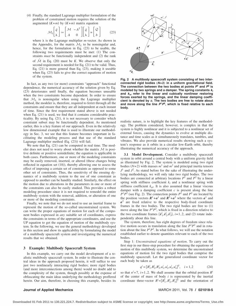
3.1 Model Development. Consider a multibody spacecraftsystem in orbit around a central body with a uniform gravity fieldas illustrated by Fig. 2. The system is modeled using two rigidbodies �N=2� with masses m1 and m2 and principal inertia tensorsJ1 and J2. As stated before for the sake of illustrating the under-lying methodology, we will only take two rigid bodies. The twobodies are connected at arbitrary locations P1 and P2 by a linearspring with stiffness coefficient kl and a nonlinear spring withstiffness coefficient knl. It is also assumed that a linear viscousdamper with a damping coefficient c is present along the lineP1P2 �see Fig. 2�. The connection points P1 and P2 are located bythe position vectors R1+a1 and R2+a2 where the vectors a1 anda2 are fixed relative to the respective body-fixed coordinateframes in the two bodies. The two rigid bodies are free to �1�move along the line P1P2, which is fixed in a direction relative tothe two coordinate frames ��1

i ,�2i ,�3

i �, i=1,2, and �2� rotate inde-pendently about this line.

The system, therefore, has eight degrees of freedom since rela-tive motion occurs in translation along the line P1P2 and in rota-tion about the line P1P2. In what follows, we will use the notationestablished earlier to denote quantities relevant to each of the twobodies.

Step 1: Unconstrained equations of motion. To carry out thefirst step in our three-step procedure for obtaining the equations ofmotion of this multibody system, we determine the unconstrainedequations of motion for the two rigid bodies that comprise themultibody spacecraft. Let the generalized coordinate vector foreach body be taken as

qi = �R1i ,R2

i ,R3i ,u1

i ,u2i ,u3

i ,u4i �T, i = 1,2 �24�

so that ni=7, i=1,2. We shall assume that the orbital position Ri

of the center of mass of body i is represented by the inertiali i i i T

c

lk

1 1,m J

2 2,m J

1R

2R

3R1R

2R

1a

12εεεε

1P11εεεε

13εεεε

23εεεε

22εεεε

21εεεε

2P 2anlk

Fig. 2 A multibody spacecraft system consisting of two inter-connected rigid bodies „N=2… in a uniform gravitational field.The connection between the two bodies at points P1 and P2 ismodeled by two springs and a damper. The spring constants kland knl refer to the linear and cubically nonlinear restoringforces exerted by the springs, and the linear damping coeffi-cient is denoted by c. The two bodies are free to rotate aboutand move along the line P1P2, which is fixed relative to eachbody.

coordinate three-vector R = �R1 ,R2 ,R3� and the orientation of

MARCH 2011, Vol. 78 / 021018-5


b=

Wcbfp

r

T�

w

Tg

Tegt

wpms

Itb

Tf

w

HErot

0

Downlo

ody i is represented by the unit quaternion four-vector ui

�u1i ,u2

i ,u3i ,u4

i �T. By a unit quaternion, we mean

�ui�Tui = 1, i = 1,2 �25�

e note that the number of coordinates chosen to describe theonfiguration of each of the two bodies that constitute the multi-ody system exceeds six, the minimum number needed and, there-ore, the seven coordinates chosen in Eq. �24� cannot all be inde-endent of one another.

The rotation matrix Si �Eq. �1�� associated with body i is pa-ameterized by the quaternion ui as

Si�ui� = �u2i u1

i − u4i u3

i

u3i u4

i u1i − u2

i

u4i − u3

i u2i u1

i ��u2

i u3i u4

i

u1i − u4

i u3i

u4i u1

i − u2i

− u3i u2

i u1i� �26�

herefore, the chosen generalized coordinates Ri and ui �see Eqs.5� and �7�� yield the corresponding matrices �see Eqs. �6� and �8��

Gi = I3i , i = 1,2 �27�

Hi = 2Ei, i = 1,2 �28�

here the matrix Ei is the 3 by 4 matrix given by

Ei = �− u2i u1

i u4i − u3

i

− u3i − u4

i u1i u2

i

− u4i u3

i − u2i u1

i � �29�

he angular velocity of body i in its body-fixed reference frame isiven by Eq. �8� so that

�i = 2Eiui �30�

he generalized force-torque vectors Qi= ��i�T , ��i�T�T, i=1,2,xerted on the individual bodies are generated by the presence ofravitational, elastic, and damping forces. The uniform gravita-ional potential of body i is

Ugi �Ri� = −

�gmi

�Ri�, i = 1,2 �31�

here � · � denotes the two-norm operation and the gravitationalarameter �g is the product of the gravitational constant and theass of the Earth. The elastic potential of the linear and nonlinear

pring is given by

Ue�q� =1

2kl��D� − �e�2 +

1

4knl��D� − �e�4 �32�

n Eq. �32�, �e is the unstretched length of the two springs be-ween the points P1 and P2, and the relative distance vector Detween the points P1 and P2 is given by

D = R1 + a1 − R2 − a2 �33�

he viscous damping is described by the Rayleigh dissipationunction

Ud�q, q� =1

2cD · D �34�

here

D = R1 + �1 � a1 − R2 − �2 � a2 �35�

ere, we note that the components of the vectors Ri, �i, and ai inqs. �33� and �35� are all to be resolved in a consistent frame of

eference. Using Eqs. �31�, �32�, and �34�, the generalized forcesn body i, assuming no “impressed forces” are applied to it, are,
hus,
21018-6 / Vol. 78, MARCH 2011


�i = −�Ug

i

�Ri −�Ue

�Ri −�Ud

�Ri, i = 1,2 �36�

Similarly, the generalized torques on body i, assuming no “im-pressed torques” are applied to it, are

�i = −�Ue

�ui −�Ud

� ui, i = 1,2 �37�

The first step in our approach is accomplished by usingLagrange’s equation under the key assumption that each of thecomponents of the generalized coordinate vectors qi, i=1,2, areindependent of the others, �see Eq. �11��. This gives

Mi�q�qi = Qi�q, q�, i = 1,2 �38�

where

Mi = �miI3i 0

0 4�Ei�TJiEi , Qi = � �i

− 8ETJEu + �i , i = 1,2

�39�

The expressions for some of the individual terms of �i and �i areinordinately long and have not, for brevity, been given here. Theunconstrained equations of motion for the two bodies are, thus,obtained as �see Eq. �14��

Mq ª �M1 0

0 M2 �q1

q2 = �Q1

Q2 ª Q �40�

where M is a 14 by 14 matrix and the vector Q is a 14-vectorsince K=14.

This first step illustrates the following three important featuresof the method. �1� The ease with which these equations can bewritten; this is because we have used far more coordinates �a totalof 14� to describe the configuration of the system than the mini-mum number required, which is eight. �2� Lagrange’s equationsare determined under the assumption that all the coordinates areindependent of one another. �3� The matrix M in Eq. �40� issingular because 4�Ei�TJiEi is singular, which is a consequence ofthe prior two features.

Step 2: Description of constraints. We next impose the neces-sary constraints on the two rigid bodies that are a consequence of

�i� not having used the minimum number of coordinates todescribe the configuration of each body

�ii� not yet having expressed the proper interconnections be-tween the two bodies in our unconstrained equations ofmotion

The method does not impose any restrictions on the number �ornature� of constraints to be used; the modeler can include what-ever constraints are decipherable, irrespective of whether they areindependent or not.

Thus, we have the two required unit quaternion constraints �seeEq. �15��

�11 = �u1�Tu1 − 1 = 0 �41�

and

�12 = �u2�Tu2 − 1 = 0 �42�

which are required so that the quaternions u1 and u2 represent realphysical rotations.

In addition, we have the modeling constraints due to the physi-cal interaction of the two bodies. This interaction is governed bythe requirement that the direction of the relative distance vector Dis fixed relative to the two body-fixed coordinate frames. This
requirement is modeled by the modeling constraint equations


Tladsh

Icwr

imgveE

bosi��otesOtssc

scmstSms

stslao

T=ettwb

J

Downlo

n1 � D = 0 and n2 � D = 0 �43�

he unit vectors n1 and n2 in Eq. �43� are determined by theocations of the spring and damper connections at the points P1

nd P2 �see the numerical example in the next subsection for theirescription�. Equation �43� leads, in general, to a total of six con-traints, one for each component of the cross product, so that weave the set of constraints �see Eq. �16��

�k�q� = 0, k = 1,2, . . . ,6 �44�

t is important to point out that Eq. �43� is an intuitive modelingonstraint, which is a modeling requirement that is easily derivedhen mentally constructing the multibody system from the two

igid bodies.Now, by appropriately differentiating each of the m=8 model-

ng constraint equations with respect to time, we can form theodeling constraint matrix equation as in Eq. �18�. This process

enerates an 8 by 14 matrix A whose rank is six, and an eight-ector b. For ease of implementation, this differentiation can beasily carried out symbolically using platforms like MAPLE, MATH-

MATICA, or MATLAB.Step 3: Determination of the equations of motion of the multi-

ody system. At this point we have all the information needed tobtain both the explicit acceleration of the multibody spacecraftystem and the explicit force of constraint needed to satisfy themposed modeling constraint set. We simply use the UP equationEqs. �21� and �22��, which is valid because the UP rank condition

the matrix M �Eq. �20�� has full rank� is satisfied with the rank

f M being 14. The fact that this matrix has full rank implies thathe generalized acceleration can be uniquely found, which is nec-ssary for obtaining the equations of motion of the multibodyystem and is also a useful check on the validity of our modeling.n the other hand, were the standard Lagrange multiplier method

o be used �see Eq. �23��, it would fail since the matrix ML isingular. Finally, since the equations of motion of the multibodyystem are directly and explicitly found, it is simple to numeri-ally implement them using a standard ode solver.

As we shall shortly see, the nonlinear spacecraft system de-cribed in this section has complex dynamical behavior: it in-ludes translational, tumbling, and vibrational motion, as well asultiple characteristic time scales ranging from several thousand

econds to a few tens of seconds, and multiple characteristic dis-ance scales ranging from several thousand kilometers to 10−4 m.uch nonlinear, multiscale systems are often difficult to accuratelyodel and usually pose considerable challenges from a numerical

tandpoint.

3.2 Numerical Results. We now provide numerical resultshowing the response of the modeled multibody spacecraft sys-em. The initial conditions of the two-body spacecraft systemhown in Fig. 3 are specified so that the system is in a circularow-Earth orbit where the center of mass of body 1 is at a constantltitude of 300 km. The mass mi and the principal inertia matrix Ji

f each component body i are given by

m1 = 2200 kg �45�

J1 = diag�2300, 4500, 3600� kg m2 �46�

m2 = 1200 kg �47�

J2 = diag�1700, 2000, 600� kg m2 �48�

he linear and nonlinear elastic spring constants are kl25 N m−1 and knl=1 N m−3, respectively, and the damping co-fficient is taken to be c=0.2 N m−1 s. The equilibrium length ofhe spring is �e=2 m. The spring connections are located relativeo the two spacecraft by the position vectors a1 and a2 �see Fig. 3�hose components in the body-fixed frame of reference are given
y the three-vectors


a1 = �1, 0, 1�T m �49�and

a2 = �− 1, 0, 1�T m �50�The components of the initial position and velocity vectors in theinertial frame are

R1�0� = �RE + 300,0,0�T km �51�

R1�0� = �0, ��g/R11�0�, 0�T km s−1 �52�

R2�0� = �RE + 300.004,0,0�T km �53�

R2�0� = �0, ��g/R11�0�, 0�T km s−1 �54�

where the gravitational parameter �g=3.986�105 km3 s−2 andRE=6378.1 km is the equatorial radius of Earth. Thus, initially,the distance between the two masses is 4 m; the springs are un-stretched, and the distance between them is 2 m �see Fig. 3�. Thevelocities in Eqs. �52� and �54� correspond to the required velocityfor an equatorial circular orbit. The initial rotational state is cho-sen so that

u1�0� = u2�0� = �1, 0, 0, 0�T �55�

u1�0� = u2�0� = �0, 0, 0, 0�T �56�

Given the spring connection locations a1 and a2 in Eqs. �49� and�50� and the initial position and orientation of the two bodies, therequired components of the unit vectors n1 and n2 expressed inthe respective body-fixed reference frames of the two bodies aresimply �see Fig. 3�

n1 = �1, 0, 0�T �57�and

n2 = �1, 0, 0�T �58�The numerical integration of the multibody spacecraft systemfound by Eq. �21� is carried out for a time duration t� �0,16293� s using a variable time step Runge–Kutta schemewith a relative error tolerance of 10−10 and an absolute error tol-erance of 10−13. The duration of integration corresponds to ap-proximately three orbital periods.

In order to check the fidelity of our multibody model, whosedescription is provided by the equations of motion obtained instep three of our methodology, our attention must first be drawn tothe extent to which all the modeling constraints are satisfied. Thenumerically integrated equations of motion must result in these

2P

1P

2a

1a

1 1,m J

2 2,m J

12εεεε

1 11 ˆ=εεεε n

13εεεε

23εεεε 2

2εεεε

2 21 ˆ=εεεε n

c

lk

nlk

1R

2R

3R

2m

2m

2m

Fig. 3 A view illustrating the initial configuration of the system

constraints being satisfied, or else our model would be deficient.

MARCH 2011, Vol. 78 / 021018-7


Tpagcws

FsssFttFtppmp

pTcb

Ft=s

0

Downlo

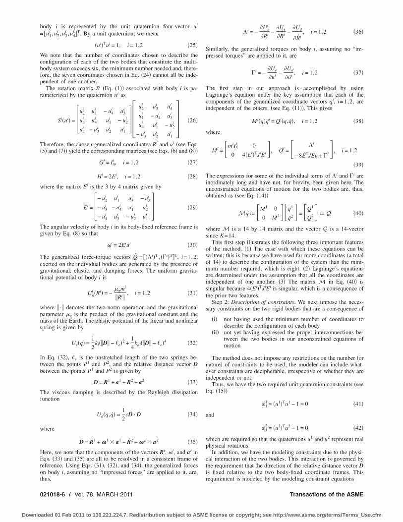
o investigate this, we show in Figs. 4�a� and 4�b� the superim-osed plots of the errors in the modeling constraints �1

i , i=1,2,nd �k, k=1,2 , . . . ,6, respectively, over the duration of the inte-ration. Noting the vertical scales, we find that all eight modelingonstraints are satisfied better than the local error tolerances usedhen numerically integrating our modeled multibody spacecraft

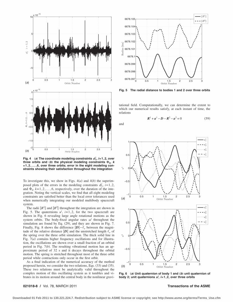
ystem.The radii �R1� and �R2� throughout the integration are shown in

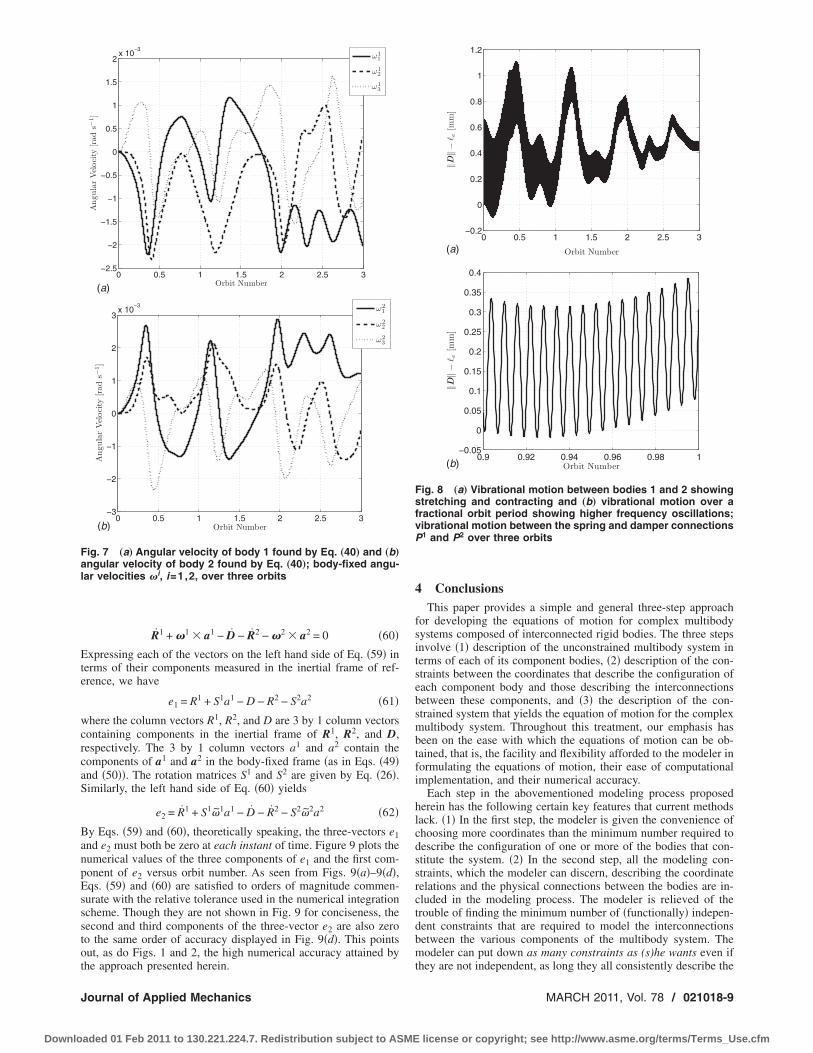
ig. 5. The quaternions ui, i=1,2, for the two spacecraft arehown in Fig. 6 revealing large angle rotational motions as theystem orbits. The body-fixed angular rates �i throughout theimulation are found by Eq. �29�, and they are shown in Fig. 7.inally, Fig. 8 shows the difference �D�−�e between the magni-

ude of the relative distance �D� and the unstretched length �e ofhe spring over the three orbit simulation. The thick solid line inig. 7�a� contains higher frequency oscillations and for illustra-

ion, the oscillations are shown over a small fraction of an orbitaleriod in Fig. 7�b�. The resulting vibrational motion has an ap-roximate period of 32 s and it decays throughout the orbitalotion. The spring is stretched throughout most of the three orbit

eriod while contractions only occur in the first orbit.As a final indication of the numerical accuracy of the method

roposed herein, we consider the two relations, Eqs. �33� and �35�.hese two relations must be analytically valid throughout theomplex motion of this oscillating system as it tumbles and vi-

0 0.5 1 1.5 2 2.5 3

−5

0

5

10x 10

−15

Orbit Number

φi 1

i=

1,2

(a)

0 0.5 1 1.5 2 2.5 3−2

−1.5

−1

−0.5

0

0.5

1

1.5

2x 10

−12

Orbit Number

Φk

k=

1,2,

...,

6

(b)

ig. 4 „a… The coordinate modeling constraints �1i , i=1,2, over

hree orbits and „b… the physical modeling constraints �k, k1,2, . . . ,6, over three orbits; error in the eight modeling con-traints showing their satisfaction throughout the integration

rates in its motion around the central body in the nonlinear gravi-

21018-8 / Vol. 78, MARCH 2011


tational field. Computationally, we can determine the extent towhich our numerical results satisfy, at each instant of time, therelations

R1 + a1 − D − R2 − a2 = 0 �59�and

0 0.5 1 1.5 2 2.5 36678.097

6678.098

6678.099

6678.1

6678.101

6678.102

6678.103

6678.104

6678.105

Orbit Number

Rad

ius

[km

]

‖R1‖‖R2‖

Fig. 5 The radial distance to bodies 1 and 2 over three orbits

0 0.5 1 1.5 2 2.5 3−1

−0.5

0

0.5

1

Orbit Number

u1

u11

u12

u13

u14

(a)

0 0.5 1 1.5 2 2.5 3−1

−0.5

0

0.5

1

Orbit Number

u2

u21

u22

u23

u24

(b)

Fig. 6 „a… Unit quaternion of body 1 and „b… unit quaternion ofi
body 2; unit quaternions u , i=1,2, over three orbits


Ete

wcrcaS

BanpEssstot

Fal

J

Downlo

R1 + �1 � a1 − D − R2 − �2 � a2 = 0 �60�xpressing each of the vectors on the left hand side of Eq. �59� in

erms of their components measured in the inertial frame of ref-rence, we have

e1 = R1 + S1a1 − D − R2 − S2a2 �61�

here the column vectors R1, R2, and D are 3 by 1 column vectorsontaining components in the inertial frame of R1, R2, and D,espectively. The 3 by 1 column vectors a1 and a2 contain theomponents of a1 and a2 in the body-fixed frame �as in Eqs. �49�nd �50��. The rotation matrices S1 and S2 are given by Eq. �26�.imilarly, the left hand side of Eq. �60� yields

e2 = R1 + S1�1a1 − D − R2 − S2�2a2 �62�

y Eqs. �59� and �60�, theoretically speaking, the three-vectors e1nd e2 must both be zero at each instant of time. Figure 9 plots theumerical values of the three components of e1 and the first com-onent of e2 versus orbit number. As seen from Figs. 9�a�–9�d�,qs. �59� and �60� are satisfied to orders of magnitude commen-urate with the relative tolerance used in the numerical integrationcheme. Though they are not shown in Fig. 9 for conciseness, theecond and third components of the three-vector e2 are also zeroo the same order of accuracy displayed in Fig. 9�d�. This pointsut, as do Figs. 1 and 2, the high numerical accuracy attained by

0 0.5 1 1.5 2 2.5 3−2.5

−2

−1.5

−1

−0.5

0

0.5

1

1.5

2x 10

−3

Orbit Number

Angula

rVel

oci

ty[rad

s−1]

ω11

ω12

ω13

0 0.5 1 1.5 2 2.5 3−3

−2

−1

0

1

2

3x 10

−3

Orbit Number

Angula

rVel

oci

ty[rad

s−1]

ω21

ω22

ω23

(a)

(b)

ig. 7 „a… Angular velocity of body 1 found by Eq. „40… and „b…ngular velocity of body 2 found by Eq. „40…; body-fixed angu-ar velocities �i, i=1,2, over three orbits

he approach presented herein.



4 ConclusionsThis paper provides a simple and general three-step approach

for developing the equations of motion for complex multibodysystems composed of interconnected rigid bodies. The three stepsinvolve �1� description of the unconstrained multibody system interms of each of its component bodies, �2� description of the con-straints between the coordinates that describe the configuration ofeach component body and those describing the interconnectionsbetween these components, and �3� the description of the con-strained system that yields the equation of motion for the complexmultibody system. Throughout this treatment, our emphasis hasbeen on the ease with which the equations of motion can be ob-tained, that is, the facility and flexibility afforded to the modeler informulating the equations of motion, their ease of computationalimplementation, and their numerical accuracy.

Each step in the abovementioned modeling process proposedherein has the following certain key features that current methodslack. �1� In the first step, the modeler is given the convenience ofchoosing more coordinates than the minimum number required todescribe the configuration of one or more of the bodies that con-stitute the system. �2� In the second step, all the modeling con-straints, which the modeler can discern, describing the coordinaterelations and the physical connections between the bodies are in-cluded in the modeling process. The modeler is relieved of thetrouble of finding the minimum number of �functionally� indepen-dent constraints that are required to model the interconnectionsbetween the various components of the multibody system. Themodeler can put down as many constraints as (s)he wants even if

(a)0 0.5 1 1.5 2 2.5 3

−0.2

0

0.2

0.4

0.6

0.8

1

1.2

Orbit Number

‖D‖−

� e[m

m]

0.9 0.92 0.94 0.96 0.98 1−0.05

0

0.05

0.1

0.15

0.2

0.25

0.3

0.35

0.4

Orbit Number

‖D‖−

� e[m

m]

(b)

Fig. 8 „a… Vibrational motion between bodies 1 and 2 showingstretching and contracting and „b… vibrational motion over afractional orbit period showing higher frequency oscillations;vibrational motion between the spring and damper connectionsP1 and P2 over three orbits

they are not independent, as long they all consistently describe the

MARCH 2011, Vol. 78 / 021018-9


mPmsadmcasila

daamdtne

mp

0

Downlo

ultibody system. �3� The last step simply uses the Udwadia–hohomsiri equation to give the explicit equation of motion of theultibody dynamical system �5� and the explicit force of con-

traint required to satisfy the imposed modeling constraints. Nottention needs to be paid to whether the mass matrix is positiveefinite or semipositive definite. A check on the validity of theodeling is also provided to the modeler through the UP rank

ondition. To the best of the authors’ knowledge, no currentlyvailable general methodologies for modeling complex multibodyystems are capable of achieving these useful features collectivelyn as uniform and simple a manner. These features, which in turnead to several others that distinguish the approach from thosevailable hereto, have been explained in detail in the paper.

Besides its simplicity and effectiveness, this three-step proce-ure has a certain intuitive feel to it since it conceptually flowslong the same logical line of thinking where one would start withset of N component rigid bodies and subsequently use them toentally construct the desired multibody system through the ad-

ition of the appropriate interconnections �constraints� betweenhem, while permitting oneself the luxury of using more coordi-ates �than the minimum needed� to describe the configuration ofach component body.

The main contributions of this paper are the following.

1. The facility with which more coordinates than the minimumnumber can be used in the formulation of problems in multi-body dynamics. Using more generalized coordinates thannecessary to describe the configuration of one or more of thecomponent bodies can often provide greater convenienceand flexibility to the modeler, especially when dealing withcomplex systems. However, this leads, in general, to a massmatrix M that may not be positive definite, but rather posi-tive semidefinite. Our ability to directly deal with such ma-

0 0.5 1 1.5 2 2.5 3−5

−2.5

0

2.5

5x 10

−13

Orbit Number

e 1(2

)

3

e 1(1

)

0 0.5 1 1.5 2 2.5−5

−2.5

0

2.5

5x 10

−13

Orbit Number(a)

(b)

Fig. 9 „a… Error in the first component of e1, „b… ethird component of e1, and „d… error in the first co

trices in the formulation of the equations of motion for

21018-10 / Vol. 78, MARCH 2011


multibody systems ultimately rests on deeper results fromanalytical dynamics, specifically the recently developed UPequation for constrained systems �5�.

2. The initial assumption that all the coordinates are indepen-dent greatly simplifies writing Lagrange’s equations for thecomponent bodies and especially the determination of thegeneralized force-torque vector.

3. Having chosen more than the minimum number of coordi-nates to facilitate her/his formulation, the modeler is pro-vided information on the suitability of her/his choice of co-ordinates by the UP rank condition �5�. This condition

requires that the matrix M= �M AT� has full rank K �equalto the number of its rows� so that the final, resulting accel-eration of the multibody system at each instant of time isunique, a requirement based on physical observations of themotion of mechanical systems.

4. The freedom to model a multibody system by using model-ing constraints that may be functionally dependent or redun-dant is an aspect that can have considerable value in increas-ing the ease with which a complex multibody system ismodeled. The modeler would indeed be required to identifythe functionally dependent constraints if �s�he uses standardLagrange multiplier methods. This is because these methodsfail when functionally dependent constraints are used. Theapproach developed in this paper is seamlessly used in thesesituations.

5. Sensitivity of the ensuing dynamics to the removal/addition/alteration of constraints can be easily carried out because noreformulations of the entire system are required, as are oftennecessary in other approaches.

6. From an implementation point of view, the approach appears

0 0.5 1 1.5 2 2.5 3−3

−2

−1

0

1

2

3x 10

−19

Orbit Number

e 1(3

)

0 0.5 1 1.5 2 2.5 3−6

−4

−2

0

2

4

6x 10

−16

Orbit Number

e 2(1

)

(c)

(d)

r in the second component of e1, „c… error in theonent of e2; errors e1 and e2 versus orbit number

rro

amenable to parallelization, and this may open up new com-



A

�s

w

aw

h

Pg

fsfi

J

Downlo

putational approaches when dealing with large-scale, com-plex multibody systems.

7. The example of a realistic interconnected two-body space-craft in a low-Earth orbit illustrates all the key features ofthe modeling approach presented herein, including its easeof use and its accuracy. The dynamics of the nonlinear sys-tem is complex as it undergoes translation, tumbling, andvibration at multiple time and distance scales. The numericalresults show that all the constraints are well satisfied. In fact,they are numerically satisfied �see Figs. 1 and 2� to orders ofmagnitude commensurate with the relative error toleranceused in the numerical integration of the equations of motion.

8. The modeling approach developed herein yields an explic-itly generated set of equations of motion for multibody sys-tems that are simple to construct, easy to computationallyimplement, and yield numerically accurate results.

ppendixWe prove here that the �K+m� by �K+m� matrix ML in Eq.

23� is nonsingular if and only if the following two conditions areatisfied.

�1� the rank of the m by K matrix A is m�2� the rank of the matrix M= �M AT� is K

here the matrix M is positive definite or positive semidefinite.Proof. �a� Let us assume that the two requirements stated above

re satisfied. We shall show that the matrix ML is nonsingular. Alle need to show then is that the equation

ML�

� ª �M − AT

A 0 �

� = �0

0 �A1�

as one and only one solution =�=0. Equation �A1� implies that

M = AT�

A = 0 �A2�

remutiplying the first of these by T and using the second, weet

TM = �A �T� = 0 �A3�

rom which it follows that M1/2 =0 since M is positiveemidefinite �or positive definite�. Hence, M =0. Thus, by therst equation in relation �A2� we must have AT�=0, and since the



rank of AT is m, the unique solution of this equation is �=0.Equation �A1� then becomes

MT = �MA = 0 �A4�

whose unique solution is =0, since the rank of MT is K.�b� Let us now assume that the matrix ML is nonsingular. Then,

the columns of the matrix ML must be linearly independent.

Thus, the submatrix MT, which has K columns, must have rankK; similarly, the submatrix �−A 0�T, which has m columns, must

have rank m. Hence, the rank of M is K and the rank of A is m.

References�1� Udwadia, F. E., and Kalaba, R. E., 1992, “A New Perspective on Constrained

Motion,” Proc. R. Soc. London, Ser. A, 439, pp. 407–410.�2� Udwadia, F. E., and Kalaba, R. E., 1993, “On Motion,” J. Franklin Inst., 330,

pp. 571–577.�3� Udwadia, F. E., and Kalaba, R. E., 1996, Analytical Dynamics: A New Ap-

proach, Cambridge University Press, New York.�4� Udwadia, F. E., and Kalaba, R. E., 2002, “On the Foundations of Analytical

Dynamics,” Int. J. Non-Linear Mech., 37, pp. 1079–1090.�5� Udwadia, F. E., and Phohomsiri, P., 2006, “Explicit Equations of Motion for

Constrained Mechanical Systems With Singular Mass Matrices and Applica-tions to Multi-Body Dynamics,” Proc. R. Soc. London, Ser. A, 462, pp. 2097–2117.

�6� Kane, T. R., and Levinson, D. A., 1980, “Formulation of Equations of Motionfor Complex Spacecraft,” J. Guid. Control, 3�2�, pp. 99–112.

�7� Schiehlen, W. O., 1984, “Dynamics of Complex Multibody Systems,” SMArch., 9. pp. 159–195.

�8� Featherstone, R., 1987, Robot Dynamics Algorithms, Kluwer, New York.�9� Bae, D. S., and Haug, E. J., 1987, “A Recursive Formulation for Constrained

Mechanical System Dynamics: Part II Closed Loop Systems,” Mech. Struct.Mach., 15�4�, pp. 481–506.

�10� Critchley, J. H., and Anderson, K. S., 2003, “A Generalized Recursive Coor-dinate Reduction Method for Multibody Dynamic Systems,” Int. J. MultiscaleComp. Eng., 1�2–3�, pp. 181–200.

�11� Shabana, A. A., 1998, Dynamics of Multibody Systems, Cambridge UniversityPress, New York.

�12� Nikravesh, P. E., 1988, Computer-Aided Analysis of Mechanical Systems,Prentice-Hall, Englewood Cliffs, NJ.

�13� Pradhan, S., Modi, V. J., and Misra, A. K., 1997, “Order N Formulation forFlexible Multibody Systems in Tree Topology: Lagrangian Approach,” J.Guid. Control Dyn., 20�4�, pp. 665–672.

�14� Hemami, H., and Weimer, F. C., 1981, “Modeling of Nonholonomic DynamicSystems With Applications,” ASME J. Appl. Mech., 48, pp. 177–182.

�15� Borri, M., Bottasso, C. L., and Mantegazza, P., 1992, “Acceleration ProjectionMethod in Multibody Dynamics,” Eur. J. Mech. A/Solids, 11�3�, pp. 403–418.

�16� Udwadia, F. E. and Schutte, A. D., 2010, “An Alternative Derivation of theQuaternion Equations of Motion for Rigid-Body Rotational Dynamics,”ASME J. Appl. Mech., 77�4�, p. 044505.

MARCH 2011, Vol. 78 / 021018-11


Date post:	30-Jul-2018
Category:	Documents
Upload:	lamkhue
View:	214 times
Download:	0 times

New Approach to the Modeling of Complex Multibody...

Documents