1521-0103/372/1/136–147$35.00 https://doi.org/10.1124/jpet.119.264143THE JOURNAL OF PHARMACOLOGY AND EXPERIMENTAL THERAPEUTICS J Pharmacol Exp Ther 372:136–147, January 2020Copyright ª 2019 by The American Society for Pharmacology and Experimental Therapeutics

Commentary

New Author Guidelines for Displaying Data and Reporting DataAnalysis and Statistical Methods in Experimental Biology

Martin C. Michel, T.J. Murphy, and Harvey J. MotulskyDepartment of Pharmacology, Johannes Gutenberg University, Mainz, Germany (M.C.M.); Partnership for the Assessment andAccreditation of Scientific Practice, Heidelberg, Germany (M.C.M.); Department of Pharmacology and Chemical Biology, EmoryUniversity, Atlanta, Georgia (T.J.M.); and GraphPad Software, Los Angeles, California (H.J.M.)

Received November 22, 2019; accepted November 22, 2019

ABSTRACTThe American Society for Pharmacology and ExperimentalTherapeutics has revised the Instructions to Authors for DrugMetabolism and Disposition, Journal of Pharmacology andExperimental Therapeutics, and Molecular Pharmacology.These revisions relate to data analysis (including statisticalanalysis) and reporting but do not tell investigators how todesign and perform their experiments. Their overall focus ison greater granularity in the description of what has beendone and found. Key recommendations include the need todifferentiate between preplanned, hypothesis-testing, andexploratory experiments or studies; explanations of whetherkey elements of study design, such as sample size and choiceof specific statistical tests, had been specified before anydata were obtained or adapted thereafter; and explanation of

whether any outliers (data points or entire experiments) wereeliminated and when the rules for doing so had been defined.Variability should be described by S.D. or interquartile range,and precision should be described by confidence intervals;S.E. should not be used. P values should be used sparingly; inmost cases, reporting differences or ratios (effect sizes) withtheir confidence intervals will be preferred. Depiction of datain figures should provide as much granularity as possible,e.g., by replacing bar graphs with scatter plots whereverfeasible and violin or box-and-whisker plots when not. Thiseditorial explains the revisions and the underlying scientificrationale. We believe that these revised guidelines will lead toa less biased and more transparent reporting of researchfindings.

IntroductionNumerous reports in recent years have pointed out that

published results are often not reproducible, and that pub-lished statistical analyses are often not performed or inter-preted properly (e.g., Prinz et al., 2011; Begley and Ellis, 2012;Collins and Tabak, 2014; Freedman and Gibson, 2015;National Academies of Sciences Engineering and Medicine,2019). Funding agencies, journals, and academic societieshave addressed these issues with best practice statements,guidelines, and researcher checklists (https://acmedsci.ac.uk/file-download/38189-56531416e2949.pdf; Jarvis and Wil-liams, 2016).In 2014, the National Institutes of Health met with editors

of many journals and established Principles and Guidelinesfor Reporting Preclinical Research. These guidelines wererapidly adopted by more than 70 leading biomedical researchjournals, including the journals of the American Society forPharmacology and Experimental Therapeutics (ASPET). A

statement of support for these guidelines was published in theSociety’s journals (Vore et al., 2015) along with updatedInstructions to Authors (ItA). Additionally, a statistical anal-ysis commentary was simultaneously published in multiplepharmacology research journals in 2014, including The Jour-nal of Pharmacology and Experimental Therapeutics, BritishJournal of Pharmacology, Pharmacology Research & Perspec-tives, andNaunyn-Schiedeberg’s Archives of Pharmacology, tostrengthen best practices in the use of statistics in pharma-cological research (Motulsky, 2014b).In its continuing efforts to improve the robustness and

transparency of scientific reporting, ASPET has updated theportion of the ItA regarding data analysis and reporting forthree of its primary research journals, Drug Metabolism andDisposition, Journal of Pharmacology and ExperimentalTherapeutics, and Molecular Pharmacology.These ItA are aimed at investigators in experimental

pharmacology but are applicable to most fields of experimen-tal biology. The new ItA do not tell investigators how to designand execute their studies but instead focus on data analy-sis and reporting, including statistical analysis. Here, wehttps://doi.org/10.1124/jpet.119.264143.

ABBREVIATIONS: ASPET, American Society for Pharmacology and Experimental Therapeutics; CI, confidence interval; ItA, Instructions toAuthors.

136

at ASPE

T Journals on June 26, 2020

jpet.aspetjournals.orgD

ownloaded from

summarize and explain the changes in the ItA and alsoinclude some of our personal recommendations. We wish toemphasize that guidelines are just that, guidelines. Authors,reviewers, and editors should use sound scientific judgmentwhen applying the guidelines to a particular situation.

Explanation of the GuidelinesGuideline: Include Quantitative Indications of Effect

Sizes in the Abstract. The revised ItA state that theAbstract should quantify effect size for what the authors deemto be the most important quantifiable finding(s) of their study.This can be either a numerical effect (difference, percentchange, or ratio) with its 95% confidence interval (CI) ora general description, such as “inhibited by about half,”“almost completely eliminated,” or “approximately tripled.”It is not sufficient to report only the direction of a difference

(e.g., increased or decreased) or whether the differencereached statistical significance. A tripling of a response hasdifferent biologic implications than a 10% increase, even ifboth are statistically significant. It is acceptable (but notnecessary) to also include aP value in the Abstract.P values inthe absence of indicators of effect sizes should not be reportedin the Abstract (or anywhere in the manuscript) because evena very small P value in isolation does not tell us whether anobserved effect was large enough to be deemed biologicallyrelevant.Guideline: State Which Parts (if Any) of the Study

Test a Hypothesis According to a Prewritten Protocoland Which Parts Are More Exploratory. The revised ItAstate that authors should explicitly say which parts of thestudy present results collected and analyzed according toa preset plan to test a hypothesis and which were done inamore exploratorymanner. The preset plan should include allkey aspects of study design (e.g., hypothesis tested, number ofgroups, intervention, sample size per group), study execution(e.g., randomization and/or blinding), and data analysis (e.g.,any normalizing or transforming of data, rules for omittingdata, and choice and configuration of the statistical tests). Afew of these planning elements are discussed below as part ofother recommendations.All other types of findings should be considered exploratory.

This includes multiple possibilities, including the following:

• Analysis of secondary endpoints from a study that waspreplanned for its primary endpoint;

• Results from post hoc analysis of previously obtaineddata; and

• Any findings from experiments in which aspects ofdesign, conduct, or analysis have been adapted afterinitial data were viewed (e.g., when sample size has beenadapted).

A statistically significant finding has a surprisingly highchance of not being true, especially when the prior probabilityis low (Ioannidis, 2005; Colquhoun, 2014). The more un-expected a new discovery is, the greater the chance that it isuntrue, even if the P value is small. Thus, it is much easier tobe fooled by results from data explorations than by experi-ments inwhich all aspects of design, including sample size andanalysis, had been preplanned to test a prewritten hypothesis.Even if the effect is real, the reported effect sizes are likely tobe exaggerated.

Because exploratory work can lead to highly innovativeinsights, exploratory findings are welcome in ASPET journalsbut must be identified as such. Only transparency aboutpreplanned hypothesis testing versus exploratory experi-ments allows readers to get a feeling for the prior probabilityof the data and the likely false positive rate.Unfortunately, this planning rule is commonly broken in

reports of basic research (Head et al., 2015). Instead, analysesare often done as shown in Fig. 1 in a process referred to asP-hacking (Simmons et al., 2011), an unacceptable form ofexploration because it is highly biased. Here, the scientistcollects and analyzes some data using a statistical test. If theoutcome is not P , 0.05 but shows a difference or trend in thehoped-for direction, one or more options are chosen fromthe following list until a test yields a P , 0.05.

• Collect some more data and reanalyze. This will bediscussed below.

• Use a different statistical test. When comparing twogroups, switch between unpaired t test, the Welchcorrected (for unequal variances) t test, or the Mann-Whitney nonparametric test. All will have differentP values, and it isn’t entirely predictable which will besmaller (Weissgerber et al., 2015). Choosing the testwith the smallest P value will introduce bias in theresults.

• Switch from a two-sided (also called two-tailed) P valueto a one-sided P value, cutting the P value in half (inmost cases).

• Remove one or a few outliers and reanalyze. This isdiscussed in a later section. Although removal of outliersmay be appropriate, it introduces bias if this removal isnot based on a preplanned and unbiased protocol.

• Transform to logarithms (or reciprocals) and reanalyze.• Redefine the outcome by normalizing (say, dividing

by each animal’s weight) or normalizing to a differentcontrol and then reanalyze.

• Use a multivariable analysis method that compares onevariable while adjusting for differences in another.

• If several outcome variables were measured (such asblood pressure, pulse, and cardiac output), switch toa different outcome and reanalyze.

• If the experiment has two groups that can be designated“control,” switch to the other one or to a combination ofthe two control groups.

• If there are several independent predictor variables, tryfitting a multivariable model that includes differentsubsets of those variables.

• Separately analyze various subgroups (say male andfemale animals) and only report the comparison with thesmaller P value.

Investigators doing this continue to manipulate the dataand analysis until they obtain a statistically significant resultor until they run out ofmoney, time, or curiosity. This behaviorignores that the principle goal of science is to find the correctanswers to meaningful questions, not to nudge data until thedesired answer emerges.In some cases, investigators don’t actually analyze data in

multiple ways. Instead, they first look at a summary or graphof the data and then decide which analyses to do. Gelman andLoken (2014) point out that this “garden of forking paths” is

Reporting Data Analysis and Statistical Methods 137

at ASPE

T Journals on June 26, 2020

jpet.aspetjournals.orgD

ownloaded from

a form of P-hacking because alternative analysis steps would

have been chosen had the data looked different.As might be imagined, these unplanned processes artifi-

cially select for higher effect sizes and lower P values thanwould be observed with a preplanned analysis. Therefore, theItA require that the authors state their analysis methodologyin detail so that any P-hacking (or practices that borderline onP-hacking) are disclosed, allowing reviewers and readers totake this into account when evaluating the results. In manycases, it makes sense to remove outliers or to log transformdata. These steps (and others) just need to be part of a plannedanalysis procedure and not be done purely because they lowerthe P value.This guideline also ensures that any HARKing(Hypothesiz-

ing After the Result is Known. Kerr, 1998) is clearly labeled.HARKing occurs when many different hypotheses are tested(say, by using different genotypes or different drugs) andan intriguing relationship is discovered, but only the datasupporting the intriguing relationship are reported. Itappears that the hypothesis was stated before the data werecollected. This is a form of multiple comparisons in which eachcomparison risks some level of type I error (Berry, 2007). Thishas been called double dipping, as the same data are used togenerate a hypothesis and to test it (Kriegeskorte et al., 2009).Guideline: Report Whether the Sample Size Was

Determined before Collecting the Data. The methodssection or figure legends should state if the sample size wasdetermined in advance. Only if the sample size was chosen inadvance can readers (and reviewers) interpret the results atface value.It is tempting to first run a small experiment and look at the

results. If the effect doesn’t cross a threshold (e.g., P , 0.05),increase the sample size and analyze the data again. Thisapproach leads to biased results because the experimentswouldn’t have been expanded if the results of the first smallexperiment resulted in a small P value. If the first smallexperiment had a small P value and the experiment wereextended, the P value might have gotten larger. However, thiswould not have been seen because the first small P valuestopped the data collection process. Even if the null hypothesiswere true, more than 5% of such experiments would yieldP , 0.05. The effects reported from these experiments tend

to be exaggerated. The results simply cannot be interpreted atface value.Methods have been developed to adapt the sample size

based on the results obtained. The increased versatility insample size collection results in wider CIs, so larger effects arerequired to reach statistical significance (Kairalla et al., 2012;https://www.fda.gov/media/78495/download). It is fine to usethese specialized “sequential” or “adaptive” statistical techni-ques so long as the protocol was preplanned and the details arereported.Unlike the British Journal of Pharmacology requirements

(Curtis et al., 2018), equal sample sizes are not required in theASPET ItA because there are situations in which it makessense to plan for unequal sample size (Motulsky and Michel,2018). It makes sense to plan for unequal sample size whencomparingmultiple treatments to a single control. The controlshould have a larger n. It also makes sense to plan for unequalsample size when one of the treatments is much moreexpensive, time consuming, or risky than the others andtherefore should have a smaller sample size than the others.In most cases, it makes sense to have the same sample size ineach treatment group.Situations exist in which a difference in sample sizes

between groups was not planned but emerges during anexperiment. For instance, an investigator wishes to measureion currents in freshly isolated cardiomyocytes from twogroups of animals. The number of successfully isolatedcardiomyocytes suitable for electrophysiological assessmentfrom a given heart may differ for many reasons. It is alsopossible that some samples from a planned sample sizeundergo attrition, such as if more animals in the diseasedgroup die than in the control group. This difference in attritionacross groups may in itself be a relevant finding.The following are notes on sample size and power.

• Sample size calculations a priori are helpful, sometimesessential, to those planning a major experiment or tothose who evaluate that plan. Is the proposed samplesize so small that the results are likely to be ambiguous?If so, the proposed experiment may not be worth theeffort, time, or risk. If the experiment uses animals, theethical implications of sacrificing animals to a study that

Fig. 1. P-hacking refers to a series ofanalyses in which the goal is not toanswer a specific scientific question, butrather to find a hypothesis and dataanalysis method that results in a P valueless than 0.05.

138 Michel et al.

at ASPE

T Journals on June 26, 2020

jpet.aspetjournals.orgD

ownloaded from

is unlikely to provide clear results should be considered.Is the sample size so large that it is wasteful? Evaluatingthe sample size calculations is an essential part of a fullreview of a major planned experiment. However, oncethe data are collected, it doesn’t really matter how thesample size was decided. The method or justificationused to choose sample size won’t affect interpretation ofthe results. Some readers may appreciate seeing thepower analyses, but it is not required.

• Some programs compute “post hoc power” or “observedpower” from the actual effect (difference) and S.D.observed in the experiment. We discourage reporting ofpost hoc or observed power because these values can bemisleading and do not provide any information that isuseful in interpreting the results (Hoenig and Heisey,2001; http://daniellakens.blogspot.com/2014/12/observed-power-and-what-to-do-if-your.html; Lenth, 2001; Levineand Ensom, 2001).

• TheBritish Journal of Pharmacology requires a minimumof n 5 5 per treatment group (Curtis et al., 2018). The ItAdo not recommend such a minimum. We agree that inmost circumstances, a sample size ,5 is insufficient fora robust conclusion. However, we can imagine circum-stances in which the differences are large compared withthe variability, so smaller sample sizes can provide usefulconclusions (http://daniellakens.blogspot.com/2014/12/observed-power-and-what-to-do-if-your.html). This es-pecially applies when the overall conclusion will beobtained by combining data from a set of different typesof experiments, not just one comparison.

Guideline: Provide Details about Experimental andAnalytical Methods. The methods section of a scientificarticle has the following two purposes:

• To allow readers to understand what the authors havedone so that the results and conclusions can beevaluated,

• To provide enough information to allow others to repeatthe study.

Based on our experience as editors and reviewers, thesegoals are often not achieved. The revised ItA emphasize theneed to provide sufficient detail in the methods section,including methods used to analyze data. In other words, thedescription of data analysis must be of sufficient granularitythat anyone starting with the same raw data and applying thesame analysis will get exactly the same results. This includesaddressing the following points.

• Which steps were taken to avoid experimental bias, e.g.,prespecification, randomization, and/or blinding? Ifapplicable, this can be a statement that such measureswere not taken.

• Have any data points or entire independent experimen-tal replicates (“outliers”) been removed from the analy-sis, and how was it decided whether a data point orexperiment was an outlier? For explanations, see thenext section.

• The full name of statistical tests should be stated, forexample, “two-tailed, paired t test” or “repeated-measuresone-way ANOVA with Dunnett’s multiple comparisonstests.” Just stating that a “t test” or “ANOVA” has beenused is insufficient. When comparing groups, it should be

stated whether P values are one or two sided (same as oneor two tailed). One-sided P values should be used rarelyand only with justification.

• The name and full version number of software used toperform nontrivial analyses of data should be stated.

We realize that including more details in the methodssection can lead to long sections that are difficult to read. Tobalance the needs of transparency and readability, generalstatements can be placed in the methods section of the mainmanuscript, whereas details can be included in an onlinesupplement.Guideline: Present Details about Whether and How

“Bad Experiments” or “Bad Values” Were Removedfrom Graphs and Analyses. The removal of outliers can belegitimate or even necessary but can also lead to type I errors(false positive) and exaggerated results (Bakker andWicherts,2014; Huang et al., 2018).Before identifying outliers, authors should consider the

possibility that the data come from a lognormal distribution,which may make a value look as an outlier on a linear but noton a logarithmic scale. With a lognormal distribution, a fewreally high values are expected. Deleting those as outlierswould lead to misleading results, whereas testing log-transformed values is appropriate (Fig. 2).If outlier removal is done by “gut feel” rather than preset

rules, it can be highly biased. Our brains come up with manyapparently good reasons why a value we do not like in the firstplace should be considered an outlier! Therefore, we recom-mend that outlier removal should be based on prespecifiedcriteria. If no such rules had been set, a person blinded togroup allocation may be less biased.The choice of the appropriate method for handling apparent

outliers depends on the specific circumstances and is up to theinvestigators. The ItA ask authors to state in the methods orresults section what quality control criteria were used toremove “bad experiments” or outliers, whether these criteriawere set in advance, and howmany bad points or experimentswere removed. It may also make sense to report in an onlinesupplement the details on every value or experiment removedas outliers, and to report in that supplement how the resultswould differ if outliers were not removed.Guideline: Report Confidence Intervals to Show

How Large a Difference (or Ratio) Was and HowPrecisely It Was Determined. When showing that a treat-ment had an effect, it is not enough to summarize the responseto control and treatment and to report whether a P value wassmaller than a predetermined threshold. Instead (or addition-ally), report the difference or ratio between the means (effectsize) and its CI. In some cases, it makes sense to report thetreatment effect as a percent change or as a ratio, but a CIshould still be provided.The CI provides a range of possible values for an estimate of

some effect size. This has the effect of quantifying the precisionof that estimate. Based on the outer limits of the CI, readers candetermine whether even these can still be considered biologi-cally relevant. For instance, a novel drug in the treatment ofobesity may lower body weight by a mean of 10%. In this field,a reduction of at least 5% is considered biologically relevant bymany. But consider two such studies with a different samplesize. The smaller study has a 95% CI ranging from a 0.5% re-duction to a 19.5% reduction. A 0.5% reduction in weight would

Reporting Data Analysis and Statistical Methods 139

at ASPE

T Journals on June 26, 2020

jpet.aspetjournals.orgD

ownloaded from

not be considered biologically relevant. Because the CIranges from a trivial effect to a large effect, the results areambiguous. The 95% CI from the larger study ranges from8% to 12%. All values in that range are biologically rele-vant effect sizes, and with such a tight confidence interval,the conclusions from the data are clearer. Both studies haveP , 0.05 (you can tell because neither 95% confidenceinterval includes zero) but have different interpretations.Reporting the CI is more informative than just the P value.When using a Bayesian approach, report credible intervalsrather than CI.Guideline: Report P Values Sparingly. One of the

most common problems we observe as statistical reviewers isoveruse of P values. Reasons to put less emphasis on P valueswere reviewed by Greenland et al. (2016) and Motulsky(2018).

• P values are often misunderstood. Part of the confusionis that the question a P value answers seems backward.The P value answers the following question: If the nullhypothesis is true (as well as other assumptions), what isthe chance that an experiment of the same size wouldresult in an effect (difference, ratio, or percent change) aslarge as (or larger than) that observed in the completedexperiment? Many scientists think (incorrectly) that theP value is the probability that a given result occurred bychance.

• Statisticians don’t entirely agree about the best use of Pvalues. The American Statistical Association publisheda statement about P values introduced by Wassersteinand Lazar (2016) and accompanied it with 21 commen-taries in an online supplement. This was not sufficient toresolve the confusion or controversy, so a special issue ofThe American Statistician was published in 2019 with 43articles and commentaries about P values introduced byWasserstein et al. (2019).

• P values are based on tentatively assuming a nullhypothesis that is typically the opposite of the biologichypothesis. For instance, when the question would bewhether the angiotensin-converting enzyme inhibitorcaptopril lowers blood pressure in spontaneously hyper-tensive rats, the null hypothesis would be that it doesnot. In most pharmacological research, the null hypoth-esis is often false because most treatments cause at leastsome change to most outcomes, although that effect maybe biologically trivial. The relevant question, therefore,is how big the difference is. The P value does not addressthis question. P values say nothing about how importantor how large an effect is. With a large sample size, the Pvalue will be tiny even if the effect size is small andbiologically irrelevant.

• Even with careful replication of a highly repeatablephenomenon, the P value will vary considerably fromexperiment to experiment (Fig. 3). P values are “fickle”(Halsey et al., 2015). It is not surprising that randomsampling of data leads to different P values in differentexperiments. However, we and many scientists weresurprised to see how much P values vary fromexperiment to experiment (over a range of more thanthree orders of magnitude). Note that Fig. 3 is the bestcase, when all variation from experiment to experimentis due solely to random sampling. If there are additionalreasons for experiments to vary (perhaps because ofchanges in reagents or subtle changes in experimentalmethods), the P values will vary even more betweenrepeated experiments.

Guideline: Dichotomous Decisions Based on a SingleP Value Are Rarely Helpful. Scientists commonly usea P value to make a dichotomous decision (the data are, orare not, consistent with the null hypothesis). There are manyproblems with doing this.

Fig. 2. Hypothetical data illustrating how data points may appear as outliers on a linear scale but not after log transformation. The five data tests areall randomly drawn from a lognormal distribution. The left panel uses a linear scale. Some of the points look like outliers. The right panel shows the samedata on a logarithmic axis. The distribution is symmetrical, as expected for lognormal data. There are no outliers.

140 Michel et al.

at ASPE

T Journals on June 26, 2020

jpet.aspetjournals.orgD

ownloaded from

• Interpretation of experimental pharmacology data oftenrequires combining evidence from different kinds ofexperiments, so it demands greater nuance than justlooking at whether a P value is smaller or larger thana threshold.

• When dichotomizing, many scientists always set thethreshold at 0.05 for no reason except tradition. Ideally,the threshold should be set based on the consequences offalse-positive and false-negative decisions. Benjaminet al. (2018) suggest that the default threshold shouldbe 0.005 rather than 0.05.

• Sometimes, the goal is to show that two treatments areequivalent. Just showing a large P value is not enoughfor this purpose. Instead, it is necessary to use specialstatistical methods designed to test for equivalence ornoninferiority. These are routinely applied by clinicalpharmacologists in bioequivalence studies.

• Many scientists misinterpret results when the P value isgreater than 0.05 (or any prespecified threshold). It isnot correct to conclude that the results prove there is “no

effect” of the treatment. The corresponding confidenceinterval quantifies how large the effect is likely to be.With small sample sizes or large variability, the P valuecould be greater than 0.05, even though the differencecould be large enough to be biologically relevant(Amrhein et al., 2019).

• When dichotomizing, many scientists misinterpretresults when the P value is less than 0.05 or anyprespecified threshold. One misinterpretation is believ-ing that the chance that a conclusion is a false positive isless than 5%. That probability is the false-positive rate.Its value depends on the power of the experiment andthe prior probability that the experimental hypothesiswas correct, and it is usually much larger than 5%.Because it is hard to estimate the prior probability, it ishard to estimate the false positive rate. Colquhoun(2019) proposed flipping the problem by computing theprior probability required to achieve a desired false-positive rate. Another misinterpretation is that a P valueless than 0.05 means the effect was large enough to be

Fig. 3. Variability of P values. If the null hypothesis is true, then the distribution of P values is uniform. Half the P values will be less than 0.50, 5% willbe less than 0.05, etc. But what if the null hypothesis is false? The figure shows data randomly sampled from two Gaussian populations with the S.D.equal to 5.0 and populations means that differ by 5.0. Top: three simulated experiments. Bottom: the distribution of P values from 2500 such simulatedexperiments. Not counting the 2.5% highest and lowest P values, the middle 95% of the P values range from 0.00016 to 0.73, a range covering almost3.5 orders of magnitude!

Reporting Data Analysis and Statistical Methods 141

at ASPE

T Journals on June 26, 2020

jpet.aspetjournals.orgD

ownloaded from

biologically relevant. In fact, a trivial effect can lead toa P value less than 0.05.

In an influential Nature paper, Amrhein et al. (2019)proposed that scientists “retire” the entire concept of makingconclusions or decisions based on a single P value, but thisissue is not addressed in the ASPET ItA.To summarize, P, 0.05 does not mean the effect is true and

large, and P . 0.05 does not prove the absence of an effect orthat two treatments are equivalent. A single statisticalanalysis cannot inform us about the truth but will alwaysleave some degree of uncertainty. One way of dealing with thisis to embrace this uncertainty, express the precision of theparameter estimates, base conclusions on multiple lines ofevidence, and realize that these conclusions might be wrong.Definitive conclusions may only evolve over time with multi-ple lines of evidence coming from multiple sources. Data canbe summarized without pretending that a conclusion has beenproven.Guideline: Beware of the Word “Significant.”. The

word “significant” has two meanings.

• In statistics, it means that a P value is less than a presetthreshold (statistical a).

• In plain English, it means “suggestive,” “important,” or“worthy of attention.” In a pharmacological context, thismeans an observed effect is large enough to havephysiologic impact.

Both of these meanings are commonly used in scientificpapers, and this accentuates the potential for confusion. Asscientific communication should be precise, the ItA suggestsnot using the term “significant” (Higgs, 2013; Motulsky,2014a).If the plain English meaning is intended, it should be

replaced with one of many alternative words, such as “impor-tant,” “relevant,” “big,” “substantial,” or “extreme.” If thestatistical meaning is intended, a better wording is “P ,0.05” or “P , 0.005” (or any predetermined threshold), whichis both shorter and less ambiguous than “significant.”Authors who wish to use the word “significant” with itsstatistical meaning should always use the phrase “statisti-cally significant.”Guideline: Avoid Bar Graphs. Because bar graphs only

show two values (mean and S.D.), they can be misleading.Very different data distributions (normal, skewed, bimodal, or

with outliers) can result in the same bar graph (Weissgerberet al., 2015). Figure 4 shows alternatives to bar graphs (seeFigs. 7–9 for examples for smaller data sets). The preferredoption for small samples is the scatter plot, but this kind ofgraph can get cluttered with larger sample sizes (Fig. 4). Inthese cases, violin plots do a great job of showing the spreadand distribution of the values. Box-and-whisker plots showmore detail than a bar graph but can’t show bimodaldistributions. Bar graphs should only be used to show dataexpressed as proportions or counts or when showing scatter,violin, or box plots would make the graph too busy. Examplesfor the latter include continuous data when comparing manygroups or showing X versus Y line graphs (e.g., depictinga concentration-response curve). In those cases, showingmean6 S.D. or median with interquartile range is an acceptableoption.A situation in which bar graphs are not helpful at all is the

depiction of results from a paired experiment, e.g., before-aftercomparisons. In this case, before-after plots are preferred, inwhich the data points from a single experimental unit areconnected by a line so that the pairing effects become clear (seeFig. 8). Alternately, color can be used to highlight individualreplicate groups. Authors may consider additionally plottingthe set of differences between pairs, perhaps with its meanand CI.Guideline: Don’t Show S.E. Error Bars. The ItA dis-

courage use of S.E. error bars to display variability. Thereason is simple; the S.E. quantifies precision, not variability.The S.E. of a mean is computed from the S.D. (S.D. thatquantifies variation) and the sample size. S.E. error bars aresmaller than S.D., and with large samples, the S.E. is alwaystiny. Thus, showing S.E. error bars can be misleading, makingsmall differences look more meaningful than they are, partic-ularly with larger sample sizes (Weissgerber et al., 2015)(Fig. 5).Variability should be quantified by using the S.D. (which

can only be easily interpreted by assuming a Gaussiandistribution of the underlying population) or the inter-quartile range.When figures or tables do not report raw data but instead

report calculated values (differences, ratios, EC50s), it isimportant to also report how precisely those values have beendetermined. This should be done with CI rather than S.E. fortwo reasons. First, CIs can be asymmetric to better showuncertainty of the calculated value. In contrast, reporting

Fig. 4. Comparison of bar graph (mean and S.D.), box and whiskers, scatter plot, and violin plot for a large data set (n 5 1335). Based on data showingnumber of micturitions in a group of patients seeking treatment (Amiri et al., 2018). Note that the scale of the y-axis is different for the bar graph than forthe other graphs.

142 Michel et al.

at ASPE

T Journals on June 26, 2020

jpet.aspetjournals.orgD

ownloaded from

a single S.E. cannot show asymmetric uncertainty. Second,although a range extending from the computed value minusone S.E. to that value plus one S.E. is sort of a CI, its exactconfidence level depends on sample size. It is better to reporta CI with a defined confidence level (usually 95% CI).Guideline: ASPET Journals Accept Manuscripts

Based on the Question They Address and the Qualityof the Methods and Not Based on Results. Althoughsome journals preferentially publish studies with a “positive”result, the ASPET journals are committed to publishingpapers that answer important questions irrespective ofwhether a “positive” result has been obtained, so long as themethods are suitable, the sample size was large enough, andall controls gave expected results.Why not just publish “positive results,” as they are more

interesting than negative results?

• Studies with robust design, e.g., those including ran-domization and blinding, have a much greater chance offinding a “neutral” or “negative” outcome (Sena et al.,2007; MacLeod et al., 2008). ASPET doesn’t want todiscourage the use of the best methods because they aremore likely to lead to “negative” results.

• Even if there is no underlying effect (of the drug orgenotype), it is possible that some experiments will endup with statistically significant results by chance. If onlythese studies, but not the “negative” ones, get published,there is selection for false positives. Scientists oftenreach conclusions based on multiple studies, eitherinformally or by meta-analysis. If the negative resultsare not published, scientists will only see the positiveresults and be misled. This selection of positive results injournals is called “publication bias” (Dalton et al., 2016).

• If there is a real effect, the published studies willexaggerate the effect sizes. The problem is that results

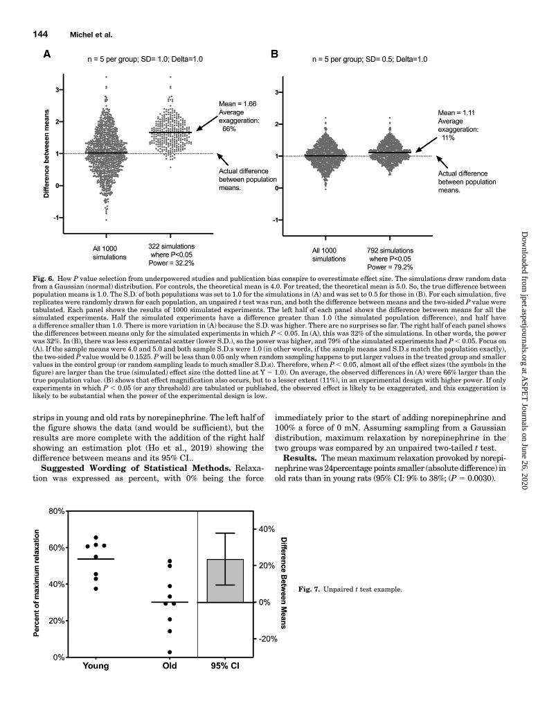
will vary from study to study, even with the sameunderlying situation. When random factors make theeffect large, the P value is likely to be ,0.05, so thepaper gets published. When random factors makethe effect small, the P value will probably be .0.05,and that paper won’t get published. Thus, journals thatonly publish studies with small P values select forstudies in which random factors (as well as actualfactors) enhance the effect seen. So, publication biasleads to overestimation of effect sizes. This is demon-strated by simulations in Fig. 6. Gelman and Carlin(2014) call this a Type M (Magnitude) Error.

• If journals only only accept positive results, they havecreated an incentive to find positive results, even ifP-hacking is needed. If journals accept results thatanswer relevant questions with rigorous methodology,they have created an incentive to ask importantquestions and answer them with precision and rigor.

It is quite reasonable for journals to reject manuscriptsbecause the methodology is not adequate or because thecontrols do not give the expected results. These are notnegative data but rather bad data that cannot lead to anyvalid conclusions.

Examples of How to Present Data and ResultsThe examples below, all using real data, show how we

recommend graphing data and writing the methods, results,and figure legends.

Example: Unpaired t Test

Figure 7 shows a reanalysis of published data (Frazier et al.,2006) comparing maximum relaxation of urinary bladder

Fig. 5. Comparison of error bars. Based on Frazier et al. (2006) showing maximum relaxation of rat urinary bladder by norepinephrine in young and oldrats; the left panel shows the underlying raw data for comparison as scatter plot.

Reporting Data Analysis and Statistical Methods 143

at ASPE

T Journals on June 26, 2020

jpet.aspetjournals.orgD

ownloaded from

strips in young and old rats by norepinephrine. The left half ofthe figure shows the data (and would be sufficient), but theresults are more complete with the addition of the right halfshowing an estimation plot (Ho et al., 2019) showing thedifference between means and its 95% CI..Suggested Wording of Statistical Methods. Relaxa-

tion was expressed as percent, with 0% being the force

immediately prior to the start of adding norepinephrine and100% a force of 0 mN. Assuming sampling from a Gaussiandistribution, maximum relaxation by norepinephrine in thetwo groups was compared by an unpaired two-tailed t test.Results. Themeanmaximum relaxation provoked by norepi-

nephrinewas24percentagepoints smaller (absolute difference) inold rats than in young rats (95% CI: 9% to 38%; (P 5 0.0030).

Fig. 6. How P value selection from underpowered studies and publication bias conspire to overestimate effect size. The simulations draw random datafrom a Gaussian (normal) distribution. For controls, the theoretical mean is 4.0. For treated, the theoretical mean is 5.0. So, the true difference betweenpopulation means is 1.0. The S.D. of both populations was set to 1.0 for the simulations in (A) and was set to 0.5 for those in (B). For each simulation, fivereplicates were randomly drawn for each population, an unpaired t test was run, and both the difference between means and the two-sided P value weretabulated. Each panel shows the results of 1000 simulated experiments. The left half of each panel shows the difference between means for all thesimulated experiments. Half the simulated experiments have a difference greater than 1.0 (the simulated population difference), and half havea difference smaller than 1.0. There is more variation in (A) because the S.D. was higher. There are no surprises so far. The right half of each panel showsthe differences between means only for the simulated experiments in which P, 0.05. In (A), this was 32% of the simulations. In other words, the powerwas 32%. In (B), there was less experimental scatter (lower S.D.), so the power was higher, and 79% of the simulated experiments had P, 0.05. Focus on(A). If the sample means were 4.0 and 5.0 and both sample S.D.s were 1.0 (in other words, if the sample means and S.D.s match the population exactly),the two-sided P value would be 0.1525. Pwill be less than 0.05 only when random sampling happens to put larger values in the treated group and smallervalues in the control group (or random sampling leads to much smaller S.D.s). Therefore, when P, 0.05, almost all of the effect sizes (the symbols in thefigure) are larger than the true (simulated) effect size (the dotted line at Y 5 1.0). On average, the observed differences in (A) were 66% larger than thetrue population value. (B) shows that effect magnification also occurs, but to a lesser extent (11%), in an experimental design with higher power. If onlyexperiments in which P , 0.05 (or any threshold) are tabulated or published, the observed effect is likely to be exaggerated, and this exaggeration islikely to be substantial when the power of the experimental design is low.

Fig. 7. Unpaired t test example.

144 Michel et al.

at ASPE

T Journals on June 26, 2020

jpet.aspetjournals.orgD

ownloaded from

Figure Legend. In the left panel, each symbol shows datafrom an individual rat. The lines show group means. Theanalysis steps had been decided before we looked at the data.The right panel shows the difference between themean and its95%CI. The sample sizes were unequal at the beginning of theexperiment (because of availability), and the sample sizes didnot change during the experiment.

Example: Paired t Test

Figure 8 shows a reanalysis of published data (Okeke et al.,2019) on cAMP accumulation in CHO cells stably transfectedwith human b3-adrenoceptors pretreated for 24 hours with10 mM isoproterenol (treated) or vehicle (control) and thenrechallenged with freshly added isoproterenol.Suggested Wording of Statistical Methods. The log

Emax of freshly added isoproterenol (as calculated from a fullconcentration-response curve) was determined in each exper-iment from cells pretreated with isoproterenol or vehicle. Thetwo sets of Emax values were compared with a two-tailed ratio-paired t test (equivalent to a paired t test on log of Emax).Suggested Wording of Results. Pretreating with iso-

proterenol substantially reduced maximum isoproterenol-stimulated cAMP accumulation. The geometric mean of theratio of Emax values (pretreated with isoproterenol dividedby control) was 0.26 (95% confidence interval: 0.16 to 0.43;P 5 0.0002 in two-tailed ratio-paired t test).

Suggested Wording of Figure Legend. In the left panel,each symbol shows the Emax of isoproterenol-stimulated cAMPaccumulation from an individual experiment. Data pointsfrom the same experiment, pretreated with isoproterenolversus pretreated with vehicle, are connected by a line.Sample size had been set prior to the experiment based onprevious experience with this assay. In the right panel, eachsymbol shows the ratio from an individual experiment. Theerror bar shows the geometric mean and its 95% confidenceinterval.

Example: Nonlinear Regression

Figure 9 shows a reanalysis of published data (Michel,2014) comparing relaxation of rat urinary bladder by iso-proterenol upon a 6-hour pretreatment with vehicle or 10 mMisoproterenol.Suggested Wording of Statistical Methods. Relaxa-

tion within each experiment was expressed as percent, with0% being the force immediately prior to start of addingisoproterenol and 100% a force of 0 mN. Concentration-response curves were fit to the data of each experiment (whereX is the logarithm of concentration) based on the equation

Y5 bottom1 ðtop� bottomÞ=ð1110∧ðlogEC50 � XÞÞ

to determine top (maximum effect, Emax) and log EC50, withbottom constrained to equal zero. Note that this equation doesnot include a slope factor, which is effectively equal to one.Unweighted nonlinear regression was performed by Prism (v.8.1; GraphPad, San Diego, CA). Values of Emax and2log EC50

fit to each animal’s tissue with pretreatment with vehicle or10 mM isoproterenol were compared by unpaired, two-tailedt test.Suggested Wording of Results. Freshly added isopro-

terenol was similarly potent in bladder strips pretreated withvehicle or 10 mM isoproterenol but was considerably lesseffective in the latter. The mean difference in potency (2logEC50) between control and pretreated samples was 20.22(95% CI: 20.52 to 10.09; P 5 0.1519). The mean absolutedifference for efficacy (Emax) was 26 percentage points(95% CI: 14% to 37%; P 5 0.0005).Suggested Wording of Figure Legend. The left panel

shows mean of relaxation from all experiments and a curve fitto the pooled data (for illustration purposes only). The center

Fig. 8. Paired t test example.

Fig. 9. Nonlinear regression example.

Reporting Data Analysis and Statistical Methods 145

at ASPE

T Journals on June 26, 2020

jpet.aspetjournals.orgD

ownloaded from

and right panels show 2log EC50 and Emax, respectively, forindividual experiments. The lines show means of each group.All analysis steps and the sample size of n 5 6 per group hadbeen decided before we looked at the data. Note that the y-axisis reversed, so bottom (baseline) is at the top of the graph.

Example: Multiple Comparisons

Figure 10 is based on a reanalysis of published data (Michel,2014) comparing relaxation of rat urinary bladder by iso-proterenol upon a 6-hour pretreatment with vehicle or 10 mMisoproterenol, fenoterol, CL 316,243, or mirabegron.Suggested Wording of Statistical Methods. Relaxa-

tion within each experiment was expressed as percent, with0% being the force immediately prior to the start of addingisoproterenol and 100% a lack of contractile force (measuredtension 0 mN). Concentration-response curves were fit to thedata of each experiment (where X is logarithm of concentra-tion) based on the equation

Y5bottom1 ðtop� bottomÞ=ð11 10∧ðlogEC50 � XÞÞ

to determine top (maximum effect; Emax) and log EC50 withbottom constrained to equal zero. Note that this equation doesnot include a slope factor, which is effectively equal to one.Unweighted nonlinear regression was performed by Prism (v.8.1; GraphPad). Emax and 2log EC50 values from tissue withpretreatmentwith a b-adrenergic agonist were comparedwiththose from preparations pretreated with vehicle by one-wayanalysis of variance, followed by Dunnett’s multiple compar-ison test and reporting of multiplicity-adjusted P values andconfidence intervals. As sample sizes had been adapted duringthe experiment, the P values and CIs should be considereddescriptive and not as hypothesis-testing.Suggested Wording of Results. Freshly added isopro-

terenol was similarly potent in bladder strips pretreated withvehicle or any of the b-adrenergic agonists. The Emax of freshlyadded isoproterenol was reduced by pretreatment with iso-proterenol (absolute mean difference 22 percentage points;95% CI: 6% to 39%; P 5 0.0056) or fenoterol (24% points; 8%to 41%; P 5 0.0025) but less so by pretreatment with CL316,243 (11% points;26% to 28%; P5 0.3073) or mirabegron(14% points; 21% to 29%; P 5 0.076).

Suggested Wording of Figure Legend. The left panelshows Emax for individual rats, and the lines show means ofeach group. The right panel shows the mean differencebetween treatments with multiplicity-adjusted 95% confi-dence intervals. All analysis steps had been decided beforewe looked at the data, but the sample size had been adaptedduring the course of the experiments.

SummaryThe new ItA of ASPET journals do not tell investigators how

to design and execute their studies but instead focus on dataanalysis and reporting, including statistical analysis. Some ofthe key recommendations are as follows.

• Provide details of how data were analyzed in enoughdetail so the work can be reproduced. Include detailsabout normalization, transforming, subtracting base-lines, etc. as well as statistical analyses.

• Identify whether the study (or which parts of it) wastesting a hypothesis in experiments with a prespecifieddesign, which includes sample size and data analysisstrategy, or was exploratory.

• Explain whether sample size or number of experimentswas determined before any results were obtained or hadbeen adapted thereafter.

• Explain whether statistical analysis, i.e., which specifictests to use and which groups being compared statisti-cally, was determined before any results were obtainedor had been adapted thereafter.

• Explain whether any outliers (single data points orentire experiments) were removed from the analysis. Ifso, state the criteria used and whether the criteria hadbeen defined before any results were obtained.

• Describe variability around the mean or median ofa group by reporting S.D. or interquartile range; describeprecision, e.g., when reporting effect sizes as CI. S.E.should not be used.

• Use P values sparingly. In most cases, reporting effectsizs (difference, ratio, etc.) with their CIs will besufficient.

Fig. 10. Multiple comparisons example.

146 Michel et al.

at ASPE

T Journals on June 26, 2020

jpet.aspetjournals.orgD

ownloaded from

• Make binary decisions based on a P value rarely anddefine that decision.

• Beware of the word “significant.” It can mean that a Pvalue is less than a preset threshold or that an observedeffect is large enough to be biologically relevant. Eitheravoid the word entirely (our preference) or make sure itsmeaning is always clear to the reader.

• Create graphs with as much granularity as is reasonable(e.g., scatter plots).

Acknowledgments

Work on data quality in the laboratory of M.C.M. is funded by theEuropean Quality In Preclinical Data (EQIPD) consortium as part ofthe Innovative Medicines Initiative 2 Joint Undertaking [Grant777364], and this Joint Undertaking receives support from theEuropean Union’s Horizon 2020 research and innovation programand European Federation of Pharmaceutical Industry Associations..

M.C.M. is an employee of the Partnership for Assessment andAccreditation of Scientific Practice (Heidelberg, Germany), an orga-nization offering services related to data quality. T.J.M. declares noconflict of interest inmatters related to this content.H.J.M. is founder,chief product officer, and a minority shareholder of GraphPadSoftware LLC, the creator of the GraphPad Prism statistics andgraphing software.

Authorship Contributions

Wrote or contributed to the writing of the manuscript: All authors.

References

Amiri M, Murgas S, and Michel MC (2018) Do overactive bladder symptoms exhibita Gaussian distribution? Implications for reporting of clinical trial data. NeurourolUrodyn 37 (Suppl 5):S397–S398.

Amrhein V, Greenland S, and McShane B (2019) Scientists rise up against statisticalsignificance. Nature 567:305–307.

Bakker M and Wicherts JM (2014) Outlier removal, sum scores, and the inflation ofthe Type I error rate in independent samples t tests: the power of alternatives andrecommendations. Psychol Methods 19:409–427.

Begley CG and Ellis LM (2012) Drug development: raise standards for preclinicalcancer research. Nature 483:531–533.

Benjamin DJ, Berger JO, Johannesson M, Nosek BA, Wagenmakers EJ, Berk R,Bollen KA, Brembs B, Brown L, Camerer C, et al. (2018) Redefine statistical sig-nificance. Nat Hum Behav 2:6–10.

Berry DA (2007) The difficult and ubiquitous problems of multiplicities. Pharm Stat6:155–160.

Collins FS and Tabak LA (2014) Policy: NIH plans to enhance reproducibility.Nature505:612–613.

Colquhoun D (2014) An investigation of the false discovery rate and the mis-interpretation of p-values. R Soc Open Sci 1:140216.

Colquhoun D (2019) The false positive risk: a proposal concerning what to do aboutp-values. Am Stat 73 (Suppl 1):192–201.

Curtis MJ, Alexander S, Cirino G, Docherty JR, George CH, Giembycz MA, Hoyer D,Insel PA, Izzo AA, Ji Y, et al. (2018) Experimental design and analysis and theirreporting II: updated and simplified guidance for authors and peer reviewers. BrJ Pharmacol 175:987–993.

Dalton JE, Bolen SD, and Mascha EJ (2016) Publication bias: the elephant in thereview. Anesth Analg 123:812–813.

Frazier EP, Schneider T, and Michel MC (2006) Effects of gender, age and hyper-tension on b-adrenergic receptor function in rat urinary bladder. NaunynSchmiedebergs Arch Pharmacol 373:300–309.

Freedman LP and Gibson MC (2015) The impact of preclinical irreproducibility ondrug development. Clin Pharmacol Ther 97:16–18.

Gelman A and Carlin J (2014) Beyond power calculations: assessing type S (Sign) andtype M (Magnitude) errors. Perspect Psychol Sci 9:641–651.

Gelman A and Loken E (2014) The statistical crisis in science. Am Sci 102:460–465.Greenland S, Senn SJ, Rothman KJ, Carlin JB, Poole C, Goodman SN, and AltmanDG (2016) Statistical tests, P values, confidence intervals, and power: a guide tomisinterpretations. Eur J Epidemiol 31:337–350.

Halsey LG, Curran-Everett D, Vowler SL, and Drummond GB (2015) The fickle Pvalue generates irreproducible results. Nat Methods 12:179–185.

Head ML, Holman L, Lanfear R, Kahn AT, and Jennions MD (2015) The extent andconsequences of p-hacking in science. PLoS Biol 13:e1002106.

Higgs MD (2013) Macroscope: do we really need the S-word? Am Sci 101:6–9.Ho J, Tumkaya T, Aryal S, Choi H, and Claridge-Chang A (2019) Moving beyond Pvalues: Everyday data analysis with estimation plots. Nature Methods 16:565–566,doi: 10.1038/s41592-019-0470-3.

Hoenig JM and Heisey DM (2001) The abuse of power. Am Stat 55:19–24.Huang M-W, Lin W-C, and Tsai C-F (2018) Outlier removal in model-based missingvalue imputation for medical datasets. J Healthc Eng 2018:1817479.

Ioannidis JPA (2005) Why most published research findings are false. PLoS Med 2:e124.

Jarvis MF and Williams M (2016) Irreproducibility in preclinical biomedical re-search: perceptions, uncertainties, and knowledge gaps. Trends Pharmacol Sci 37:290–302.

Kairalla JA, Coffey CS, Thomann MA, and Muller KE (2012) Adaptive trial designs:a review of barriers and opportunities. Trials 13:145.

Kerr NL (1998) HARKing: hypothesizing after the results are known. Pers SocPsychol Rev 2:196–217.

Kriegeskorte N, Simmons WK, Bellgowan PSF, and Baker CI (2009) Circular anal-ysis in systems neuroscience: the dangers of double dipping. Nat Neurosci 12:535–540.

Lenth RV (2001) Some practical guidelines for effective sample size determination.Am Stat 55:187–193.

Levine M and Ensom MHH (2001) Post hoc power analysis: an idea whose time haspassed? Pharmacotherapy 21:405–409.

Macleod MR, van der Worp HB, Sena ES, Howells DW, Dirnagl U, and Donnan GA(2008) Evidence for the efficacy of NXY-059 in experimental focal cerebral is-chaemia is confounded by study quality. Stroke 39:2824–2829.

Michel MC (2014) Do b-adrenoceptor agonists induce homologous or heterologousdesensitization in rat urinary bladder? Naunyn Schmiedebergs Arch Pharmacol387:215–224.

Motulsky H (2014a) Opinion: never use the word ‘significant’ in a scientific paper.Adv Regen Biol 1:25155.

Motulsky H (2018) Intuitive Biostatistics, 4th ed, Oxford University Press, Oxford,UK.

Motulsky HJ (2014b) Common misconceptions about data analysis and statistics.J Pharmacology and Experimental Therapeutics 351:200–205, doi: 10.1124/jpet.114.219170 25204545.

Motulsky HJ and Michel MC (2018) Commentary on the BJP’s new statisticalreporting guidelines. Br J Pharmacol 175:3636–3637.

National Academies of Sciences Engineering and Medicine (2019) Reproducibilityand Replicability in Science, The National Academies Press, Washington, DC.

Okeke K, Michel-Reher MB, Gravas S, and Michel MC (2019) Desensitization ofcAMP accumulation via human b3-adrenoceptors expressed in human embryonickidney cells by full, partial, and biased agonists. Front Pharmacol 10:596.

Prinz F, Schlange T, and Asadullah K (2011) Believe it or not: how much can werely on published data on potential drug targets? Nat Rev Drug Discov 10:712–713.

Sena E, van der Worp HB, Howells D, and Macleod M (2007) How can we improve thepre-clinical development of drugs for stroke? Trends Neurosci 30:433–439.

Simmons JP, Nelson LD, and Simonsohn U (2011) False-positive psychology: un-disclosed flexibility in data collection and analysis allows presenting anything assignificant. Psychol Sci 22:1359–1366.

Vore M, Abernethy D, Hall R, Jarvis M, Meier K, Morgan E, Neve K, Sibley DR,Traynelis S, Witkin J, et al. (2015) ASPET journals support the National Institutesof Health principles and guidelines for reporting preclinical research. J PharmacolExp Ther 354:88–89.

Wasserstein RL and Lazar NA (2016) The ASA statement on p-values: context,process, and purpose. Am Stat 70:129–133.

Wasserstein RL, Schirm AL, and Lazar NA (2019) Moving to a world beyond “p ,0.05”. Am Stat 73:1–19.

Weissgerber TL, Milic NM, Winham SJ, and Garovic VD (2015) Beyond bar and linegraphs: time for a new data presentation paradigm. PLoS Biol 13:e1002128.

Address correspondence to: Dr. Harvey J. Motulsky, GraphPad Software,1100 Glendon Ave., 17th floor, Los Angeles, CA 90024. E-mail: hmotulsky@graphpad.com

Reporting Data Analysis and Statistical Methods 147

at ASPE

T Journals on June 26, 2020

jpet.aspetjournals.orgD

ownloaded from