New Directions in Project Performance and Progress Evaluation

i

New Directions in Project Performance and Progress Evaluation

A thesis submitted to fulfil the requirements for the Degree of Doctor of Project Management

By

Douglas C. Bower

B.Arch., MBA, MSc

School of Construction, Property and Project Management RMIT University

Melbourne, Australia

July 2007

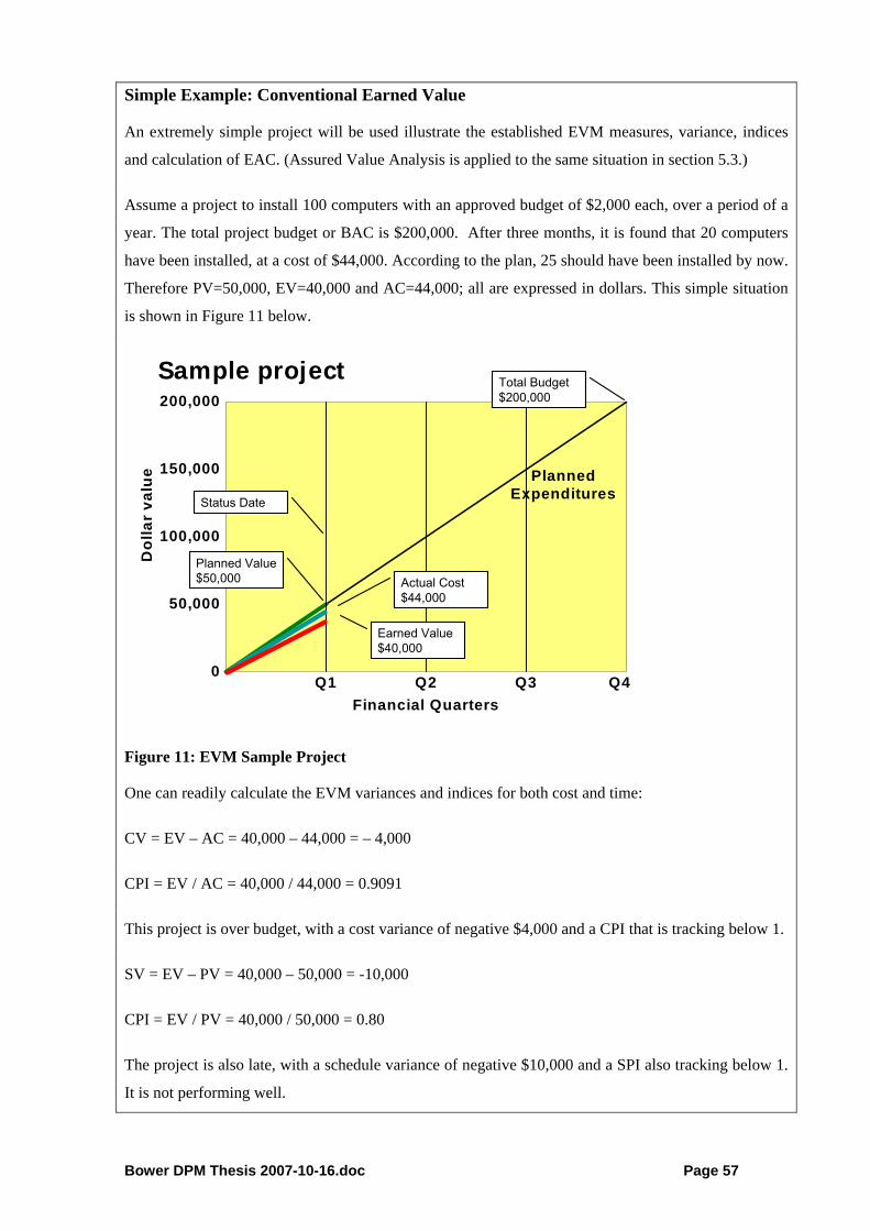
ii

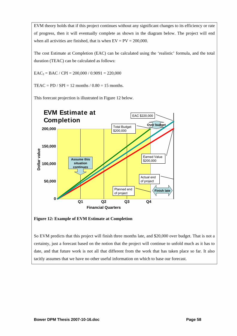
Certification I, Douglas C. Bower, do hereby certify for this thesis that: a) Except where due acknowledgement has been made, the

work is that of myself alone; b) The work has not been submitted previously, in whole or in

part, to qualify for any other academic award; c) The content of the thesis is the result of work which has

been carried out since the official commencement date of the approved research program; and

d) That any editorial work, paid or unpaid, carried out by a

third party is acknowledged.

9 August 2007 Certified by Douglas C. Bower Date

iii

Acknowledgements I would like to acknowledge the following people without whom this work could not have been completed: Derek Walker – for inviting and challenging me at the outset of this endeavour Andrew Finegan – for providing ongoing guidance and advice throughout my journey Hanita Braun – for supporting and reassuring me during these many years in my pursuit of this goal

iv

Abstract

Earned value management (EVM) is a project performance evaluation technique that has origins in

industrial engineering, but which has been adapted for application in project management. EVM is

widely recognised as a core project management technique with obvious benefits; however, its

utilisation is not widespread beyond a few specific industries, notably the defence and aerospace

organisations in the United States. I have sought to identify the reasons for this limited adoption, and

to develop improvements to EVM with the potential to increase its rate of adoption.

This study comprises four types of research: (1) comprehensive literature review, (2) survey of

representative attitudes, (3) development and testing of new model extensions to EVM, and (4)

confirmation of the validity of those new models, through multiple techniques.

This investigation has confirmed that the literature on this subject is not broad in comparison with

other management subjects. There are only a handful of books specifically on the subject, though

EVM is addressed by almost every textbook on project management. The number of peer-reviewed

and referred journal papers on EVM is also limited.

I have prepared an abbreviated one-page survey on attitudes to cost control and EVM, and

administered that survey at nine project management conference presentations and seminars. The

survey results confirm that EVM is not widely adopted, and that many project managers see the

methodology as one that is overly complex and difficult to implement.

The literature review and the simple survey, taken together with my 25 years of project management

experience and several years as a university instructor, have identified a number of serious challenges

associated with conventional EVM.

• Earned value cost forecast formulae do not take into account any future vendor

agreements already formalised through procurement.

• Development of an integrated performance management baseline is very challenging for

organisations with a low level of project management maturity.

• Calculation of the Planned Value, Earned Value and Actual Cost of work packages that

are in progress can be very onerous, particularly in projects that are dynamic.

• The schedule progress indicators (SV and SPI) are counter-intuitive and possess intrinsic

anomalies that minimize their value as the project nears completion.

• EVM does not recognise project phases or key milestones as significant events.

• The future trend lines for earned value achievement and actual cost expenditures cannot be

accurately forecast and charted.

v

I addressed the first issue by creating Assured Value Analysis (AVA). This add-in process provides

two new measures, permitting improvements to EVM that take into account the added certainty

provided through procurement. Assured Value (AV) represents the budget for a future signed contract,

and Expected Cost (EC) represents the agreed cost of that contract. Those measures permit the

calculation of a Total Cost Variance that includes not only cost deviations to date, but also future ones

to which the project team is already committed. AVA also allows conventional EVM formulae to take

into account the Assured Value and Expected Cost of future signed agreements. A simple notional

project is used to demonstrate the implementation of AVA.

I resolved the remaining issues through realising that the isolation of project phases would provide a

simplified but more dependable methodology, one that also provides features not found in

conventional EVM. Significant milestones are normally planned to occur at the end of a project phase.

By assessing project performance only at the end of each completed phase, performance calculations

are significantly simplified. The Planned Value (PV) of a completed phase must be equal to the

approved budget for that phase, and the Earned Value (EV) must be equal to the PV at that point. The

Actual Cost can be readily calculated if expenditures and staff time have been recorded (or can be

attributed) to that phase. Although the project team could implement work packages and control

accounts if they so wish, those tools are not necessary with this approach. The cumulative PV, EV and

AC figures at successive phase ends are plotted on a typical EVM chart with time measured on one

axis, and resource value on the other.

My new technique, Phase Earned Value Analysis (PEVA), not only simplifies that calculation of PV,

EV and AC, but also provides benefits that are not possible with EVM. Since the planned and actual

phase completion dates are known, an intuitively simple but accurate time-based schedule variance

and schedule performance index (i.e. SVP and SPIP) can be measured. This approach possesses many

of the virtues of emerging Earned Schedule concepts, but without complex calculations using

questionable formulae.

PEVA also permits the forecasting of future phase end cost figures and phase completion dates using

the phase CPI and SPI ratios. Since PEVA employs data points having specific x-axis and y-axis

values, those can be readily plotted and trend lines identified with standard spreadsheet functions. This

is a powerful feature, as it allows key project stakeholders to visualise emerging project performance

trends as each phase is completed.

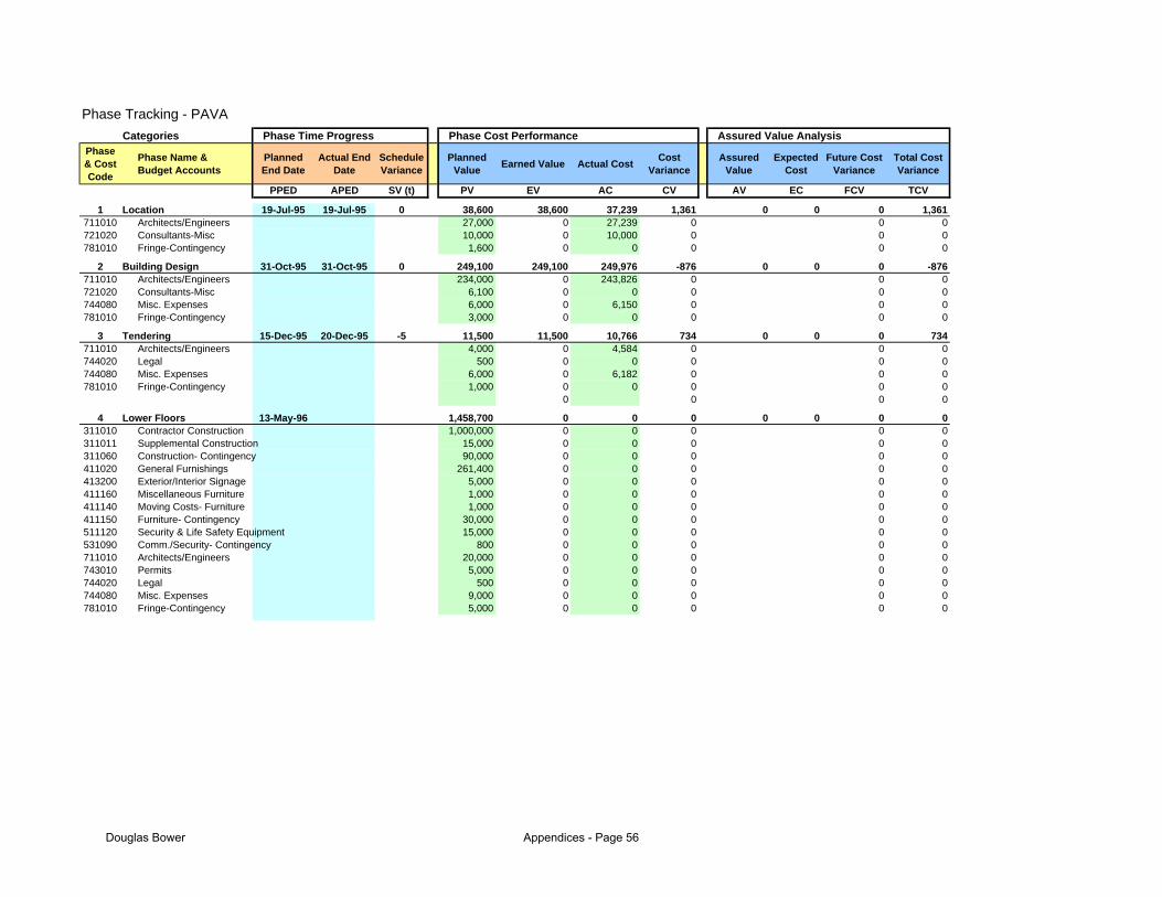
Finally, I have successfully combined the AVA and PEVA concepts, resulting in a new EVM

methodology – Phase Assured Value Analysis (PAVA) – which takes into account the assurance

provided by procurement, simplifies the calculation of earned value through phases, and provides

powerful forecasting and charting features.

vi

I have validated this new combined approach in multiple respects. The new AVA and PEVA formulae

were rigorously established and confirmed through standard algebraic procedures. The formulae were

tested in sample project situations, to clearly demonstrate their functions. I have assessed the

combined AVA and PEVA methodology in relation to the documented shortcomings of EVM, as

described in the literature and confirmed in the survey of practitioners. I have argued that the PAVA

approach conforms to the 32 criteria established in the United States for full EVM compliance. I have

presented both AVA and PEVA to critical audiences at major project management conferences in

North America and the UK, as well as several organisations, and responded to many expert criticisms

and constructive suggestions from practitioners. Finally, I have used my archived cost and schedule

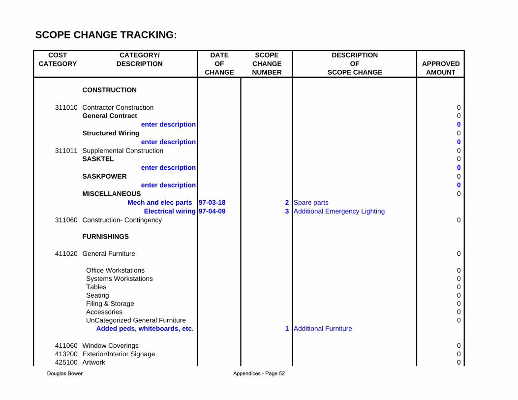
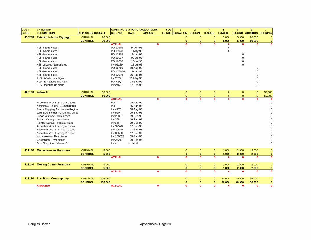
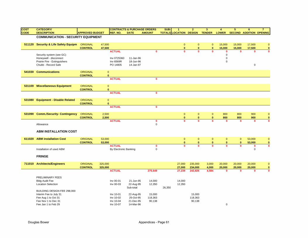
records to retrospectively test the combined PAVA methodology on a significant office facilities and

technology program, one that I completed for a large Canadian bank during the past decade.

Keywords Project management; earned value management; project phases; project performance evaluation; change management

vii

Table of Contents 1 Introduction and Justification ..........................................................................................................1

1.1 Personal Background ..............................................................................................................1 1.2 Project Performance Evaluation Context................................................................................2 1.3 Justification.............................................................................................................................5 1.4 Research Problem and Questions............................................................................................5 1.5 The Research Approach..........................................................................................................7 1.6 DPM Research Program .........................................................................................................9 1.7 Chapter Summary and Thesis Structure ...............................................................................10

2 The Supporting Literature .............................................................................................................13 2.1 Project Types ........................................................................................................................13 2.2 Project Control......................................................................................................................16 2.3 Project Phases and Scheduling .............................................................................................19 2.4 Project Uncertainty, Risk Management and EVM ...............................................................22 2.5 Chapter Summary .................................................................................................................25

3 The EVM Approach ......................................................................................................................28 3.1 Introduction...........................................................................................................................28 3.2 Origins and Evolution of EVM.............................................................................................28

3.2.1 Defining Earned Value Management ...............................................................................28 3.2.2 History of EVM development ..........................................................................................28

3.3 EVM Literature Sources .......................................................................................................30 3.3.1 General Project Management Texts .................................................................................31 3.3.2 Earned Value Specific Books...........................................................................................34 3.3.3 Journal Articles on Earned Value Management ...............................................................36

3.4 EVM Adoption and Standards ..............................................................................................37 3.4.1 Adoption by USA Government and Military ...................................................................37 3.4.2 Non-USA Governmental Adoption ..................................................................................38 3.4.3 Non-Governmental Adoption...........................................................................................39

3.5 Earned Value Methodology ..................................................................................................43 3.5.1 Earned Value Terms and Notation ...................................................................................43 3.5.2 Earned Value Measures....................................................................................................44 3.5.3 Assessment of Work Packages in Progress ......................................................................46 3.5.4 Contingency and Management Reserve ...........................................................................49 3.5.5 Cumulative and Periodic EVM Calculations....................................................................49 3.5.6 EVM Cost and Schedule Tools ........................................................................................50 3.5.7 Time Estimate at Completion...........................................................................................52 3.5.8 Cost Estimate at Completion ............................................................................................53 3.5.9 Conventional EVM Process .............................................................................................60

3.6 Time Management and Earned Value...................................................................................61 3.6.1 EVM Time Issues .............................................................................................................61 3.6.2 New Methods for Assessing Project Progress ..................................................................62

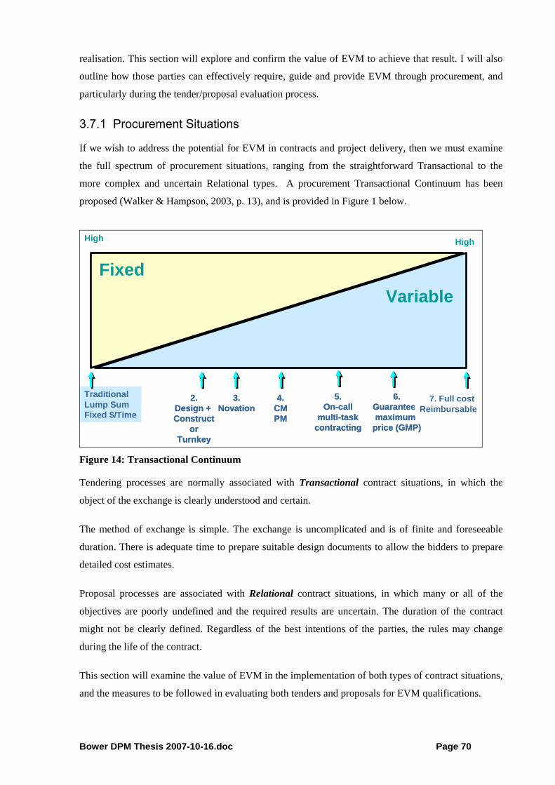
3.7 EVM Variation in Project Contracts and Delivery Scenarios...............................................69 3.7.1 Procurement Situations.....................................................................................................70 3.7.2 EVM Variation by Contract Type ....................................................................................80 3.7.3 Project Design and Delivery.............................................................................................81 3.7.4 Conclusions ......................................................................................................................86

3.8 Earned Value Management and Procurement.......................................................................86 3.8.1 Procurement and Cost Control .........................................................................................86 3.8.2 Procurement and EVM.....................................................................................................87

3.9 EVM Research Issues ...........................................................................................................88 3.10 Chapter Summary .................................................................................................................90

4 Research Design ............................................................................................................................93 4.1 Introduction to Research Design...........................................................................................93 4.2 Research Context ..................................................................................................................93 4.3 Statement of Research Plan ................................................................................................100

viii

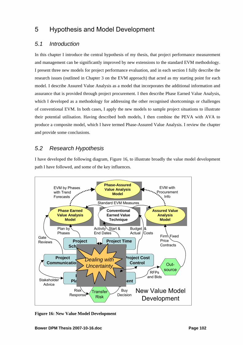
4.4 Chapter Summary ...............................................................................................................101 5 Hypothesis and Model Development ..........................................................................................102

5.1 Introduction.........................................................................................................................102 5.2 Research Hypothesis...........................................................................................................102 5.3 Assured Value Analysis......................................................................................................103

5.3.1 New Assured Value Measures: ......................................................................................104 5.3.2 Calculating the Assured Value and the Expected Cost ..................................................106 5.3.3 Proposed AVA Variances and Indices ...........................................................................107 5.3.4 Assured Value Analysis and Schedule Measures...........................................................109 5.3.5 Forecasting Cost with Assured Value Analysis .............................................................110 5.3.6 Contract Risk and Expected Cost ...................................................................................116 5.3.7 Detailed Sample AVA Application ................................................................................117

5.4 Phase Earned Value Analysis: Simplify yet Enhance EVM...............................................120 5.4.1 Earned Value Management Context...............................................................................120 5.4.2 Adapting EVM to Project Situations ..............................................................................121 5.4.3 Challenges of Standard EVM.........................................................................................122 5.4.4 The PEVA Concept ........................................................................................................130 5.4.5 Implementing PEVA ......................................................................................................138 5.4.6 PEVA Cost and Time Calculations ................................................................................140 5.4.7 Sample PEVA Project ....................................................................................................141

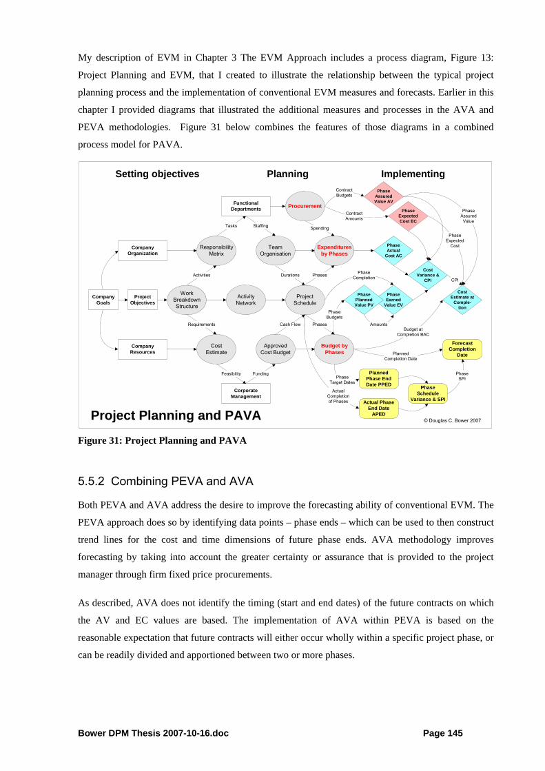
5.5 Phase Assured Value Analysis ...........................................................................................144 5.5.1 Introduction ....................................................................................................................144 5.5.2 Combining PEVA and AVA ..........................................................................................145 5.5.3 About Control Accounts in PAVA.................................................................................152 5.5.4 Implementing PAVA......................................................................................................153 5.5.5 Sample Project with Combined PEVA and AVA ..........................................................155 5.5.6 Combined Model Sample ...............................................................................................159 5.5.7 PAVA for Portfolio Management ..................................................................................161

5.6 Chapter Summary ...............................................................................................................163 6 Analysis and Discussion..............................................................................................................164

6.1 Chapter Introduction ...........................................................................................................164 6.2 Mathematical Verification ..................................................................................................164

6.2.1 AVA Mathematical Verification ....................................................................................165 6.2.2 PEVA Mathematical Verification ..................................................................................167 6.2.3 PAVA Mathematical Verification ..................................................................................168

6.3 Practitioner Evaluation .......................................................................................................170 6.3.1 Survey on Attitudes and Practices ..................................................................................170 6.3.2 Conferences and Seminars .............................................................................................172 6.3.3 PEVA Practitioner Questions .........................................................................................173 6.3.4 AVA Practitioner Questions...........................................................................................176

6.4 Comparison to EVM Standards ..........................................................................................178 6.4.1 EVM System Criteria .....................................................................................................178

6.5 Retrospective Case Analysis...............................................................................................188 6.5.1 Introduction ....................................................................................................................188 6.5.2 Demonstration Project ....................................................................................................190 6.5.3 Project Phases and Cost Records....................................................................................190 6.5.4 Validation Process ..........................................................................................................191 6.5.5 Regina Results with Formulae........................................................................................198

6.6 Chapter Summary ...............................................................................................................200 7 Conclusions .................................................................................................................................203

7.1 Introduction.........................................................................................................................203 7.2 Research Problem and Answers..........................................................................................203 7.3 Value Added by New Extensions to EVM .........................................................................206 7.4 Implications for PM practice ..............................................................................................207 7.5 Further research ..................................................................................................................208 7.6 Chapter Summary ...............................................................................................................209

ix

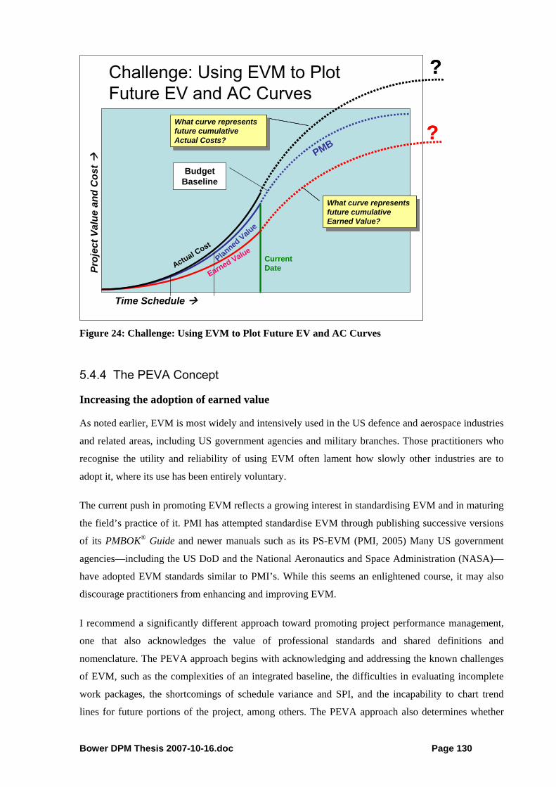
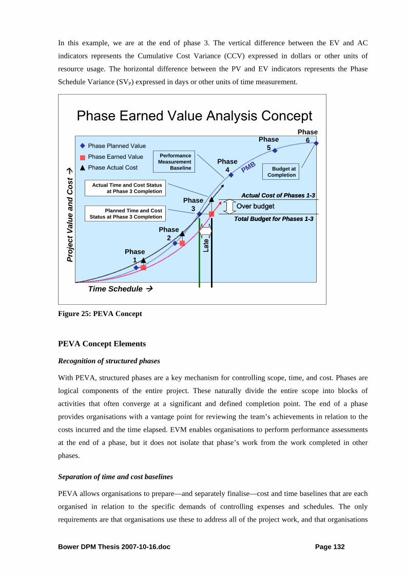
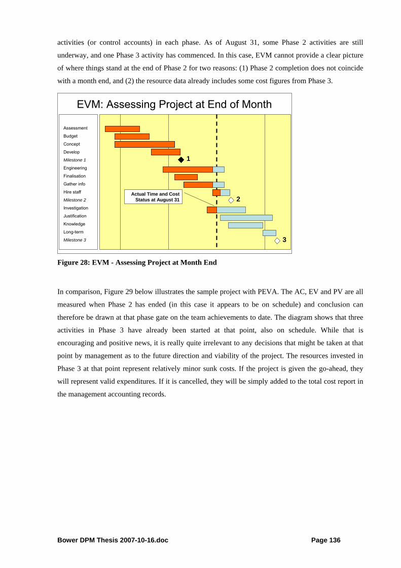
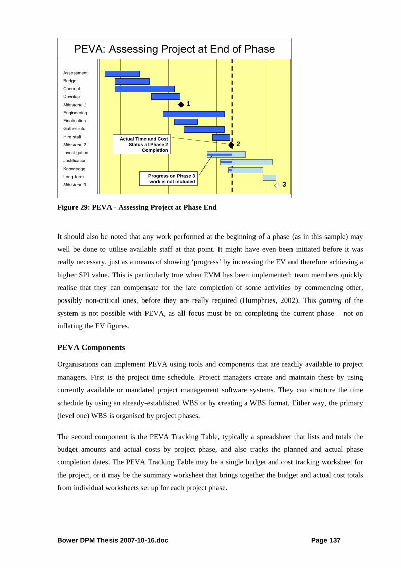
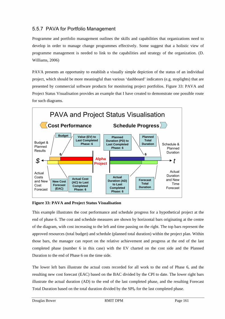
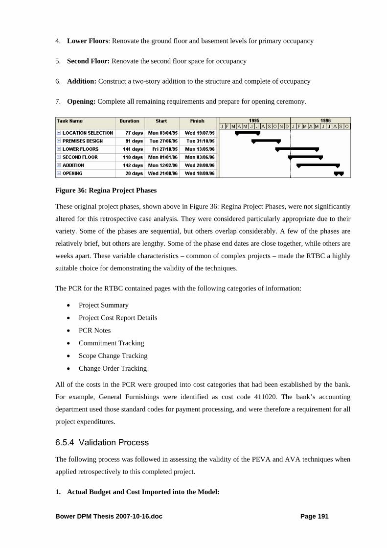
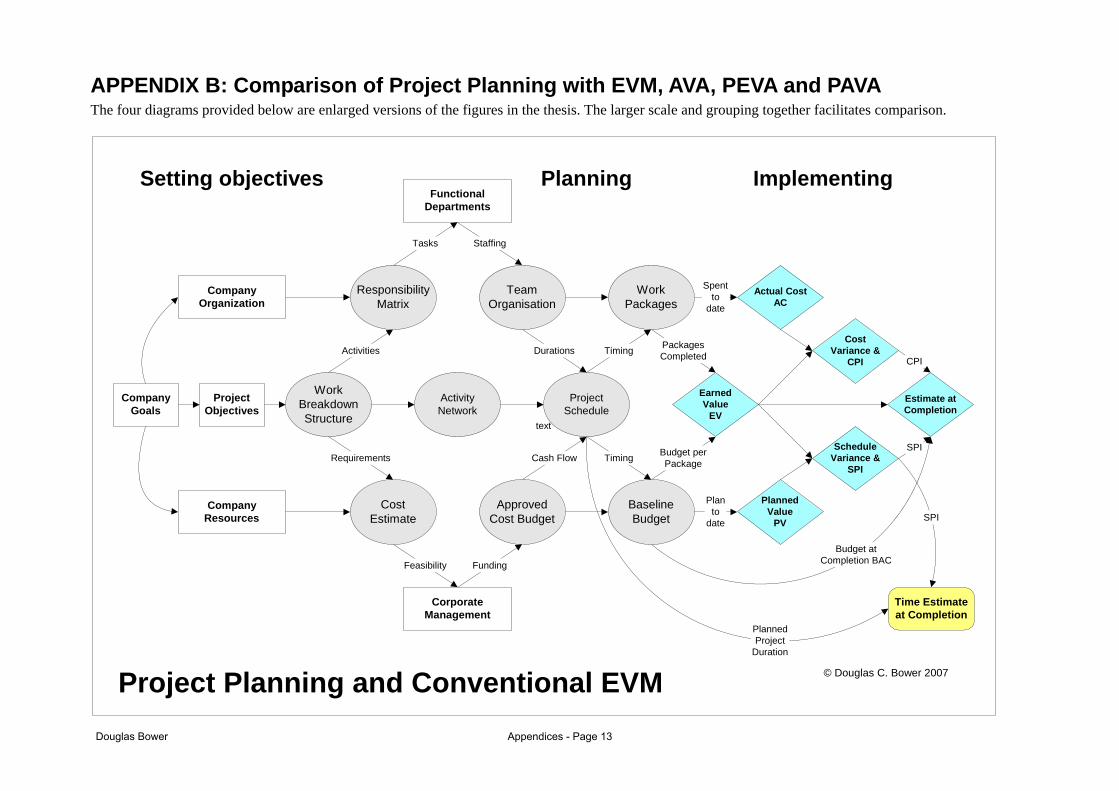
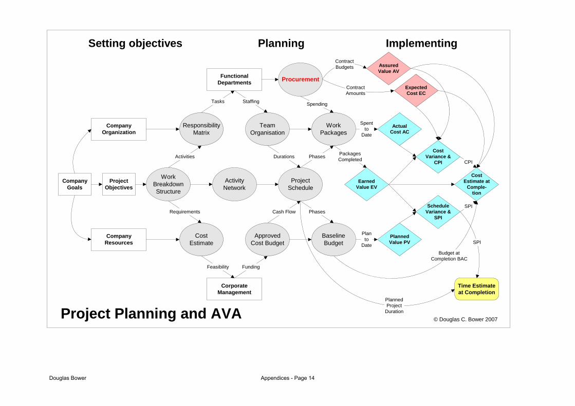
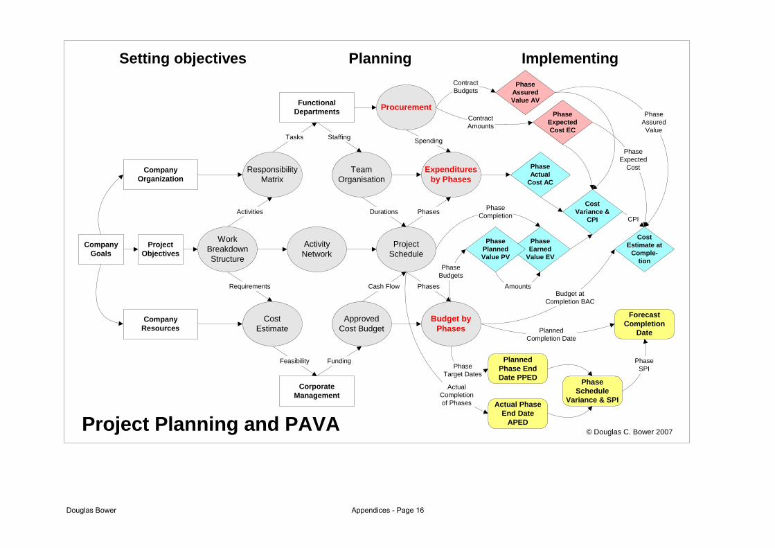
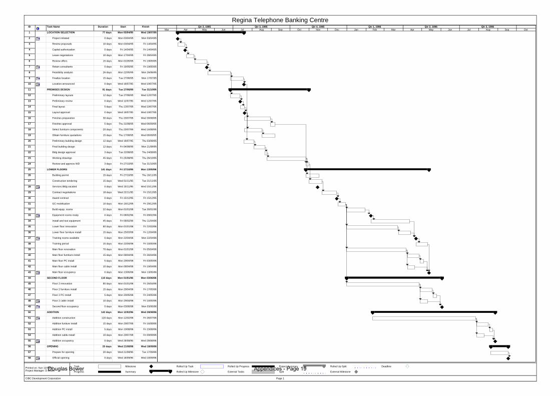
8 References ...................................................................................................................................211 9 Glossary of Terms .......................................................................................................................223 Appendices APPENDIX A: EVM Survey Results APPENDIX B: Comparison of Project Planning with EVM, AVA, PEVA and PAVA APPENDIX C: Regina Telephone Banking Centre APPENDIX D: Leading Change Through Projects APPENDIX E: Phased Rollout Projects List of Figures Figure 1: DPM Program Outline..............................................................................................................9 Figure 2: DPM Program Contribution ...................................................................................................10 Figure 3: Goals and Methods Matrix .....................................................................................................14 Figure 4: Typology of Technical Projects..............................................................................................15 Figure 5: Using Risk Analysis to Plot the PMB.....................................................................................24 Figure 6: Using Risk Analysis to Plot the EAC .....................................................................................24 Figure 7: Evolution of EVM ..................................................................................................................30 Figure 8: Integrated Performance Measurement Baseline (PMB) .........................................................45 Figure 9: Standard EV Methodology .....................................................................................................46 Figure 10: Monitoring CPI Example......................................................................................................51 Figure 11: EVM Sample Project ............................................................................................................57 Figure 12: Example of EVM Estimate at Completion ...........................................................................58 Figure 13: Project Planning and EVM ...................................................................................................60 Figure 14: Transactional Continuum......................................................................................................70 Figure 15: Research Activity as a Knowledge Creation Process ...........................................................94 Figure 16: New Value Model Development ........................................................................................102 Figure 17: Project Planning and AVA .................................................................................................104 Figure 18: Assured Value Analysis, Applied to Simple Example .......................................................114 Figure 19: Earned Value Analysis Example ........................................................................................118 Figure 20: Assured Value Analysis Example.......................................................................................119 Figure 21: EVM Cost/Time Integration Challenges ............................................................................125 Figure 22: EVM Schedule Variance Challenge ...................................................................................127 Figure 23: Applying EVM to Phase Milestones ..................................................................................128 Figure 24: Challenge: Using EVM to Plot Future EV and AC Curves................................................130 Figure 25: PEVA Concept....................................................................................................................132 Figure 26: Nine Possible PEVA Conditions ........................................................................................134 Figure 27: Project Planning and PEVA................................................................................................135 Figure 28: EVM - Assessing Project at Month End.............................................................................136 Figure 29: PEVA - Assessing Project at Phase End.............................................................................137 Figure 30: Phase Earned Value Analysis Sample Project ....................................................................143 Figure 31: Project Planning and PAVA ...............................................................................................145 Figure 32: Phase Schedule Variance ....................................................................................................150 Figure 33: PAVA and Project Status Visualisation..............................................................................161 Figure 34: PAVA and Project Portfolio Management .........................................................................162 Figure 35: Difficulty in Percent Complete Calculations ......................................................................176 Figure 36: Regina Project Phases.........................................................................................................191

x

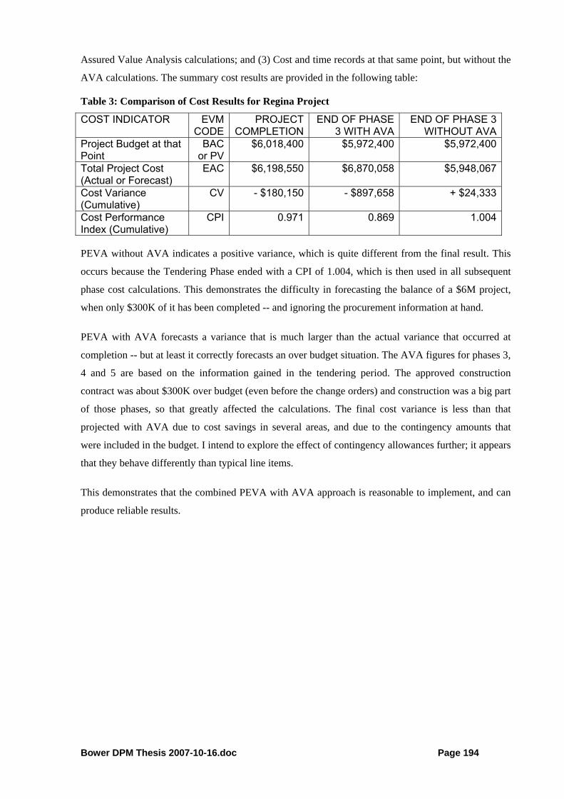
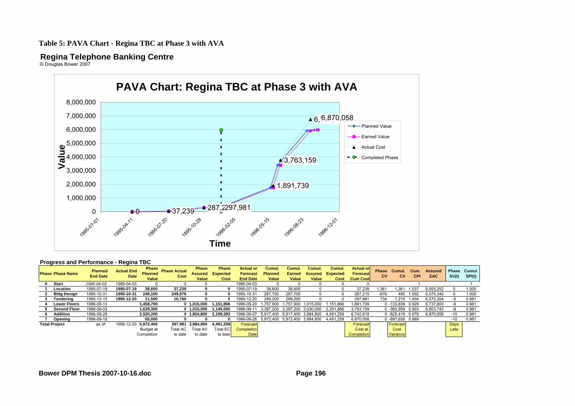
List of Tables Table 1: Elements of Project Management ............................................................................................17 Table 2: Variation in EVM Measures by Contract Type, Client Perspective ........................................81 Table 3: Comparison of Cost Results for Regina Project ....................................................................194 Table 4: PAVA Chart - Regina TBC at Completion............................................................................195 Table 5: PAVA Chart - Regina TBC at Phase 3 with AVA.................................................................196 Table 6: PAVA Chart - Regina at Phase 3 w/o AVA ..........................................................................197 Published Papers and Presentations

During the course of this doctoral program, my original work has been accepted for publication and

for presentation through the following peer-reviewed publications, international conferences and

professional seminars.

Peer Reviewed Publications Bower, D. C. (2007). Phase Earned Value Analysis: A Proposal for Simplifying yet Enhancing EVM.

The Measurable News (Spring), 7-22. Bower, D. C., Walker, D.H.T. (2007). Planning Knowledge for Phased Rollout Projects. Project

Management Journal (September). Peer Reviewed Conference Papers Bower, D. C. (2004, August 12-13). Leading Change Through Projects. Paper presented at the PMOZ

2004, Melbourne, Australia. Bower, D. C. (2004, October 23-26). Assured Value Analysis: Earned Value Extended. Paper

presented at the PMI Global Congress North America 2004, Anaheim, CA, USA. Bower, D. C. (2004, November 14-17). Assured Value Analysis: EVM Meets Procurement. Paper

presented at the 16th Annual International Integrated Program Management Conference, Tysons Corner, VA, USA.

Bower, D. C. (2005, September 10-13). Phase Earned Value Analysis. Paper presented at the PMI

Global Congress North America, Toronto, Canada. Bower, D. C. (2006, July 16-19). Phase Earned Value Analysis: A Proposal for Simplifying yet

Enhancing EVM. Paper presented at the PMI Research Conference 2006, Montreal, Canada. Peer Reviewed Conference Presentations Bower, D. C. (2005, November 29-30). Phased Rollout Projects. Presented at the PMI-OVOC /

Department of National Defence Symposium, Ottawa, Canada. (Both English and French) Bower, D. C. (2006, April 27-28). Phase Earned Value Analysis: A Proposal to Simplify yet Enhance

EVM. Presented at the Business Performance & Project Management Summit, London, UK. Bower, D. C. (2006, May 17-19) Using Phases to Improve Earned Value Performance Evaluation.

Presentation to the PMI-CPM 22nd International Conference, Clearwater Beach, Florida. (Presentation included in the conference proceedings)

xi

Bower, D. C. (2006, September 19) Phase Value as a Key to Program and Portfolio Management.

Public Sector Project Management Forum, Mississauga, Ontario. Industry Consultant Seminars Bower, D. C. (2005, October 12) Phase Earned Value Analysis, Presentation to the Nokia Group,

Los Angeles, CA. Professional Seminars and Presentations Bower, D. C. (2006, April 8) New Directions in Project Performance Evaluation. PMI Southern

Ontario Chapter Seminar, Toronto, Ontario Bower, D. C. (2006, November 18) New Directions in Project Performance Evaluation. PMI Ottawa

Valley Outaouais Chapter Seminar, Ottawa, Ontario, Bower, D. C. (2007, May 17) Why Phases are the Key to Project Performance Evaluation. Greater

Toronto Information Systems Local Interest Group, Toronto, Ontario.

xii

List of Abbreviations

The following abbreviations were utilised in this thesis. All of these terms, plus some others, are

defined in Chapter 9 Glossary of Terms. Other specialized abbreviations, not listed here, exist in the

text and are explained where they are first introduced. Terms marked (*) were developed by the

author, in the course of developing this thesis. Most other terms are in common use.

AC Actual Cost

ACP Phase Actual Cost*

ACWP Actual Cost of the Work Performed – now Actual Cost (AC)

AD Actual Duration (of the completed project)

AD Activity Description (PMI)

ANSI American National Standards Institute

APED Actual Phase End Date*

APM Association for Project Management

AT Actual Time

AV Assured Value*

AVP Phase Assured Value*

AVA Assured Value Analysis*

BAC Budget at Completion

BCWP Budgeted Cost of the Work Performed – now Planned Value (PV)

BCWP Budgeted Cost of the Work Scheduled – now Earned Value (EV)

CF Certainty Factor*

CA Control Account

CAC Cumulative Actual Cost

CAP Control Account Plan

xiii

CAV Cumulative Assured Value*

CCPI Cumulative Cost Performance Index

CCV Cumulative Cost Variance

CEC Cumulative Expected Cost*

CFC Cumulative Forecast Cost*

CPF Cost Plus Fee

CPFF Cost Plus Fixed Fee

CPI Cost Performance Index

CPIP Phase Cost Performance Index*

CPM Critical Path Method

CPV Cumulative Planned Value

CR Critical Ratio

C/SCSC Cost and Schedule Control Systems Criteria

CV Cost Variance

CVP Phase Cost Variance*

DoD Department of Defense (in the United States of America)

EAC Estimate at Completion

EC Expected Cost*

ECP Phase Expected Cost*

ED Earned Duration

EIA Electronic Industry Association

ES Earned Schedule

ETC Estimate to Complete

xiv

ETTC Estimated Time To Complete

EV Earned Value

EVP Phase Earned Value*

EVA Earned Value Analysis (synonymous with EVM)

EVM Earned Value Management

EVMS Earned Value Management System

EVT Earned Value Technique

FCPI Future Contract Performance Index*

FCV Future Cost Variance*

FD Forecast Duration*

FFP Firm Fixed Price

FPED Forecast Phase End Date*

IEAC Independent Estimate at Completion (same as EAC)

IEDAC Independent Estimate of Duration at Completion (in Earned Schedule)

LOE Level of Effort

NDIA National Defense Industry Association (USA)

OBS Organisational Breakdown Structure

PD Planned Duration* (also Project Duration)

PDM Precedence Diagramming Method

PERT Program Evaluation and Review Technique

PEVA Phase Earned Value Analysis*

PF Performance Factor

PM Project Management

xv

PMA Project Management Association (UK)

PMB Performance Measurement Baseline (also, Performance Management Baseline)

PMBOK Project Management Body of Knowledge

PMI Project Management Institute

PMO Project Management Office

PO Purchase Order

PPED Planned Phase End Date*

PSD Project Start Date

PV Planned Value

PVP Phase Planned Value*

PVRate Planned Value Rate

RFP Request for Proposal

SOW Statement Of Work

SPI Schedule Performance Index

SPI(t) Schedule Performance Index (time-based)

SPIP Phase Schedule Performance Index*

SV Schedule Variance

SVP Phase Schedule Variance*

T&M Time and Material

TACP Total Agreed Contract Price*

TCB Total Contract Budget*

TEAC Time Estimate at Completion

TCPI To-Complete Performance Index

xvi

TCV Total Cost Variance*

TV Total Variance (also Time Variance)

VAC Variance at Completion

WBS Work Breakdown Structure

* Abbreviation and term developed by Douglas Bower during this doctoral program.

Bower DPM Thesis 2007-10-16.doc Page 1

1 Introduction and Justification This chapter introduces the research topic in relation to my personal background, perspective and

experience as a practitioner, student and instructor in project management. I then review the evaluation

of project performance in the context of the project management body of knowledge, and acknowledge

some of the limitations of this topic. I provide a brief justification for this research, and then describe

my research problem and key questions. I describe my research approach, and show how it has

developed within the framework of the DPM research program. I conclude by outlining the thesis

structure as presented and developed in these seven chapters.

1.1 Personal Background

I have over 3 decades of experience in managing and directing projects and programs, in both the

public and private sectors. I have served within a wide range of organisational types: consulting firms

(architectural and engineering), government (municipal and provincial), motion picture exhibition and

entertainment, financial services, information technology services, telecommunications, and a large

urban university. I hold a Bachelor of Architecture from the University of Toronto (5-year professional

degree), a Master of Business Administration from York University in Toronto, and a Master of

Science in Telecommunications and Network Management from Syracuse University, USA. I have

taught both undergraduate and continuing education courses at Ryerson University, Toronto, in 1985-

87 and from 1998 to the present, in the areas of project management, construction management,

business information systems, and telecommunications. I was a licensed architect in the Province of

Ontario for 25 years, but my active engagement in design and construction declined during the 1990’s

as I began managing IT and telecommunications projects. I am a member of PMI and also the College

of Performance Management. I became a Project Management Professional (PMP) in 1998.

I am currently the Manager, E-Business in the Ministry of Small Business and Entrepreneurship,

Government of Ontario, Canada. In this role I lead a team delivering programs to foster the adoption

of e-business and ICT by small and medium enterprises (SMEs) as a means of increase productivity

and employment.

Although my career has spanned a wide range of project types in various industries, I have been able

to develop skills and acquire areas of knowledge which were valuable and transferable from one

challenge to the next. Those included ‘hard’ skills and knowledge for tasks such as cost estimating,

and also the ‘soft’ skills and knowledge associated with team building and leadership. I found that my

range of project management experience and the reflection-in-action (Schön, 1983) that accompanied

it was a valuable resource when teaching project management or information technology and

telecommunications topics, as it provided a wealth of examples and case studies to illustrate the

concepts and theory found in textbooks.


One key exception was in the area of project performance evaluation and control. I recognised that

earned value management (EVM) is one of the few management techniques that are unique to project

management. (For example, quality management is also used in operations.) I also realised that, even

though EVM was a standard section in every project management course and textbook, I had never

actually applied EVM – mainly because I had never been asked to do so in any of the ten organisations

where I have led or managed projects. Furthermore, it was rare for me to find a project management

colleague or mature student (enrolled in a CE evening course) who had any experience with EVM

methodology at his/her place of work.

Recognising and reflecting on this paradox led me to investigate EVM further, and to identify not only

significant issues that might be hindering its adoption – but also sound and practical improvements

that could increase its utilisation.

1.2 Project Performance Evaluation Context

Project Management Knowledge

This thesis will refer to project management knowledge mainly in relation to A Guide to the Project

Management Body of Knowledge (from this point onwards to be abbreviated to as PMBOK) that the

Project Management Institute (PMI, 2004, p. 73) has developed; it is now in its third edition. While

there are other project management bodies of knowledge, the PMI one has been the focus of this thesis

as it is the one most widely accepted in Canada, and because it has the strongest links to EVM

practices and standards. For example, PMI has published a Practice Standard for EVM (PMI, 2005) to

supplement the coverage of EVM that exists in its PMBOK.

PMBOK addresses EVM in its Chapter 7 on Project Cost Management (2004, p. 171). The section on

Cost Control identifies five tools and techniques: Cost Change Control System; Performance

Measurement Analysis; Forecasting; Project Performance Reviews; Project Management Software;

and Variance Management. Since all of those techniques are directly or indirectly related to earned

value methods, PMBOK actually devotes nearly 19 of its 21 Cost Control pages to EVM.

PMBOK refers to EVM elsewhere, but clearly it is seen as primarily as a cost control technique. Even

though PMBOK notes in its Chapter 5 on Project Time Management (2004, p. 154) briefly refers to

Performance Measurement as schedule control technique, that paragraph refers back to the Cost

Control section for details. Clearly, even PMI sees EVM as being more effective for cost control than

for schedule control. EVM is also mentioned briefly in Chapter 10 on Project Communications

Management (2004, p. 233) as a possible element of Performance Reporting and Forecasts. A sample

table is provided to illustrate the use of EVM as a reporting tool.


That chapter contains as section on how to Manage Stakeholders, but that fails to note any role for

EVM as a stakeholder communications tool. Only ‘communications methods’ and ‘issue logs’ are

recognised as common tools and techniques.

Interestingly, the previous of PMBOK (2nd edition) treated EVM slightly differently. The technique

was described in detail in Chapter 10 Project Communications Management (PMI, 2000, p. 123) and

was only referred to briefly in the chapters on Time and Cost. One must assume that EVM was seen as

mainly a communications technique for reporting on project performance to date, in the areas of both

time and cost, though even then its shortcomings in evaluating schedule progress were being realised.

In its chapter on Risk Management, the current PMBOK (3rd edition) acknowledges the link between

EVM and risk: “Earned value analysis…and other methods of project variance and trend analysis may

be used for monitoring overall project performance. Outcomes from these analyses may forecast

potential deviation of the project at completion from cost and schedule targets. Deviation from the

baseline plan may indicate the potential impact of threats or opportunities.” (PMI, 2004, p. 266)

In summary, PMBOK sees EVM as an important cost control tool that can provide useful performance

reporting and forecasts, which might broadly identify risks and opportunities. However, it is not as

effective as a schedule control technique, and is possibly too complex to be used as for stakeholder

communications.

Many organisations have adopted the management of projects, programmes and their portfolios as

their preferred approach for a wide range of initiatives related to new product development, strategy

implementation and business transformation. (Winter, Smith, Morris, & Cicmil, 2006) Despite that

progress within organisations, the conceptual base for project management theory has attracted

criticism for its lack of relevance to practice (Morris, 1994, 2000) and also for its failure to contribute

significantly to improved performance of projects across various industries.

I have questioned whether EVM – despite its prominent place in the body of project management

knowledge – is actually relevant to practice in its present form. In this thesis, I have identified some of

the shortcomings of EVM that may contribute to that lack of relevance, and to develop a stronger

conceptual base that will offer an alternative to PM practitioners interested in measuring, analysing

and enhancing their control of project activities, and thereby improving project outcomes.

Limitations of this topic

Project performance can be assessed in many different respects, and in various time dimensions.

During the project, one can measure the performance efficiency and schedule progress of project

activities (EVM) and that is the focus of this thesis. One can also measure the quality of the project

deliverables during the project, and that performance evaluation is a key element in Total Quality


Management (TQM) and other project quality initiatives. While that is a valid approach, it is not one

that is readily combined with EVM, and I have not pursued that possibility in my thesis.

I recognise the obvious link between earned value and risk management, and have noted that the

concept of combining the two techniques has been addressed by at least one author. (Hillson, 2004a)

I acknowledge that since both techniques deal with the uncertainty inherent in all projects (albeit more

in some that others) it would be advantageous to produce a combined methodology. I expect that could

be readily achieved, and I may do so in the future; however, this thesis does not do so. My objective

was to increase the adoption of EVM by addressing its known issues, providing added features, and

simplifying its utilisation. I felt that incorporating Monte Carlo simulations or other probabilistic

methods into EVM would provide a further challenge to practitioners and thereby reduce acceptance

of the core performance evaluation methodology.

One can also measure the performance of the project results, which might be term the products of the

project. For example, if the project is to create a functioning research laboratory, EVM might be used

to evaluate the performance of the construction, interior outfitting and furnishings activities while that

work is progressing. However, once the project is completed, the final EVM reports might contribute

to lessons learned, but not to the ongoing evaluation of the laboratory as an asset. At that point, the

laboratory owner would be most interested it the results of the research occurring in that laboratory,

such as completed experiments, patents obtained, journal citations for the research team, etc. On a

longer time frame, an owner such as a university or government funding agency would be is ultimately

interested in the outcomes of those laboratory results – such as reducing the incidence of a disease. In

summary, EVM is only useful in evaluating the performance and progress in delivering the immediate

products – not in evaluating either their short-term results or their long-term outcomes.

Establishing a model, possibly similar to EVM, which would evaluate results after project completion

would be an intriguing challenge, and one might envisage how that concept could be structured. For

example, one might compare the planned benefits with the actual benefits and the actual costs (both

capital and operating) to arrive at meaningful variances and indices in the period after completion of

the project deliverables. Indeed, it is possible that such calculations occur now in some industries.

However, that is not the intent of this thesis.

EVM measures the performance of the project in progress, and provides forecasts of the final results

for two key dimensions of the project – time and cost – at its completion. On that basis, EVM is seen

as a useful control and communication technique that should assist management in achieving the

successful completion of the project. However, project success does not necessarily equate with the

success of the organisation in meeting its strategic objectives. Other techniques, such as the Balanced

Scorecard approach (Kaplan & Norton, 1996) are more appropriate for that purpose.


1.3 Justification

Earned value management (EVM) is a project performance evaluation technique that has origins in

industrial engineering, but which has been adapted to project management. EVM is widely recognised

as a core project management technique with obvious benefits; however, its utilisation is not

widespread beyond a few specific industries, notably the defence and aerospace organisations in the

United States. I have sought to identify the reasons for this limited adoption, and to develop

improvements to EVM with the potential to increase its acceptance and application of the earned value

concept.

1.4 Research Problem and Questions

This research originated from my experience in teaching several project management courses in

undergraduate and in continuing education (adult learning) programs at Ryerson University in

Toronto, Canada. Introductory courses in project management, and most project management

textbooks, invariably include a section on EVM. The subject is very useful for introducing students to

the fundamental concepts of project performance and progress measurement, and prediction of project

results. EVM has also been included in the bodies of knowledge of two major project management

organisations, the Project Management Institute (PMI) and the Association for Project Management

(APM). EVM has also been mandated by several major organisations, especially governmental and

military agencies in the United States of America (USA). This general acceptance and promotion of

EVM as a best practice has been in clear contrast to the widespread ignorance or avoidance of the

practice in Canadian organisations at which I have managed and directed projects over the past two

decades.

This contradiction leads to an obvious and unavoidable paradox: EVM is widely accepted as a key PM

technique – but it is not widely used by project managers. My observation is not original; Fleming and

Koppelman (2004, p. 1) recount their conversation with the lead editor of the Harvard Business

Review, to whom they had provided information on EVM in response to his inquiry about the topic.

Apparently he wanted “assurances that EVM was for real”. After a few weeks to review that material,

the HBR editor called back and asked this key question: “If EVM is so good…why isn’t it used on all

projects?”

Fleming and Koppelman then cited three underlining reasons why, in their opinion, “EVM has not

been universally accepted on most projects”. Their first reason is that “EVM advocates often speak in

a foreign tongue”, and refer to the obtuse acronyms (e.g. BCWS) that were originally employed. This

has some validity, but it is not clear that the revised versions (e.g. PV) will make a major difference.

Their second reason is because “initially the DoD defined EVM to acquire ‘major systems’”. In other

words, EVM is meant for major defence projects – not regular ones. There is a great deal of validity to


this observation. Conventional EVM as codified in US standards may be overkill for most projects.

Thirdly, they content that “sometimes management…doesn’t really want to know the final cost!”

(Fleming & Koppelman, 2004, p. 7) This statement is borne out by the fact that EVM in the US has

been promoted mainly by financial controllers, such as those at the US federal Office of Management

and Budget (Evans, 2005), rather than by practicing project managers or directors.

If EVM is so good…why isn’t it used on all projects?

I have adopted the HBR editor’s question as the central problem in my thesis, and also addressed the

following related questions:

What is the basis and foundation of the earned value methodology?

The origins, background and current theory underlying EVM is provided as a starting point for the

discussions, analysis and propositions of the study as a whole.

To what extent is EVM utilised and accepted by project management professionals?

The current understanding and adoption of EVM by project management practitioners is examined, in

relation to alternate techniques. This study includes a summary of the recognition given to EVM by

government bodies and professional standards.

What are the strengths of EVM in the management of projects and programmes?

The study will identify the documented strengths of EVM as a project management methodology for

the evaluation of project performance and progress.

Does EVM have serious challenges, issues or flaws that may be slowing its adoption?

The study describes some of the known shortcomings of EVM, and also identifies further logical or

practical issues that may adversely affect the adoption of EVM in the profession.

What new concepts or approaches could address those challenges, and further enhance or alter EVM?

Since EVM is a relatively new methodology, it is still undergoing further refinement. Recent new

concepts are reviewed and analysed. Additional new enhancements are proposed to address the

challenges already identified.

Could those enhancements to EVM be combined to form a valid new methodology?

Enhancements to EVM could function independently, or possibly might be combined to form a

cohesive new methodology. Any such new version of earned value would need to be compatible with

current project management practices. It must also be mathematically sound, deductively logical and

consistently reliable to be considered a valid alternative.


Would a new earned value methodology be accepted by project managers?

Although EVM is a relatively straightforward concept, it has not been universally adopted by project

managers. An altered or enhanced earned value methodology would not provide any added benefit if it

was so overly complex or confusing that is was ignored by project management practitioners. To be

significant, any new or enhanced project performance evaluation methodology must represent a sound

and appropriate alternative to at least a portion of the project management profession.

1.5 The Research Approach

I have taken a multi-faceted approach in addressing these questions. I have firstly reviewed the

available academic and practitioner literature on the subject of EVM to identify perspectives that

reinforce the acceptance of EVM as a best practice, and also arguments against that prevailing

acceptance or in favour of new variations or altogether different approaches to performance

evaluation. I have also examined papers on related topics, such as risk management, knowledge

management and procurement, in order to consider how EVM relates to other key elements in project

management.

One outgrowth of this survey was my exploration of the relationships between planned change,

knowledge management and project phases. As a result of my inquiry, I developed a number of ideas

into two papers. I presented Leading Change through Projects (Bower, 2004c) at the PMOZ

Conference in Melbourne, Australia in August 2004. It explored the various ways in which project

change was delivered by projects, and also the ways that those various types of change were address

by project managers before the project initiation, in successive project phases, and after its completion.

I presented Phased Rollout Projects (Bower, 2005b) at a practitioner conference in Ottawa, Canada in

late 2005. My original papers on these two related topics are provided in Appendices E and F. I further

developed the concept of phased rollout projects with the Director of the DPM Program during 2006,

and that paper has been accepted for publication (Bower & Walker, 2007).

Based on my investigation of the EVM and related literature, I identified a number of gaps or

anomalies in EVM that appeared to both diminish its effectiveness and discourage its acceptance as a

project performance management tool. For example, EVM has been seen mainly as a cost tool due to

the low reliability of its schedule progress indicators (SV and SPI) and completion date forecasting.

To respond to those perceived shortcomings, I created new concepts and models that extended

conventional EVM methodology. My first new concept, Assured Value Analysis (AVA), included

new measures that allowed me to factor in the added certainty provided by procurement in the

forecasting of the expected total project cost or estimate at completion (EAC). My second concept,

Phase Earned Value Analysis (PEVA) used the simple and accepted framework of project phases to


resolve a number of the other EVM issues. Finally, I combined those two models into a unified new

methodology, Phase Assured Value Analysis (PAVA).

I have used my new AVA and PEVA methodologies as the basis for a series of presentations and

papers that I have delivered at project management conferences, seminars and meetings in North

America and the UK during 2004 to 2007 (see Published Papers and Presentations above). The

purposes of those presentations and papers were intended to (1) confirm that my new concepts were

original; (2) obtain practitioner questions, comments and criticisms that would aid in further

refinement of the models; and (3) contribute to the validation of the individual and combined models

as practical tools.

In order to collect some basic information on current practices, and also the opinions of practitioners

towards EVM and procurement, I developed and delivered a simple one-page survey (more of a straw

poll) that could be quickly completed by project managers attending the various conferences that I

have spoken at in the past three years. I did not intend the survey to be statistically valid or conclusive.

That said, the poll provided not only some useful indicators, but also a medium for attendees to

provide qualitative feedback on their experiences with EVM, plus some direct opinions on my new

concepts (AVA and PEVA).

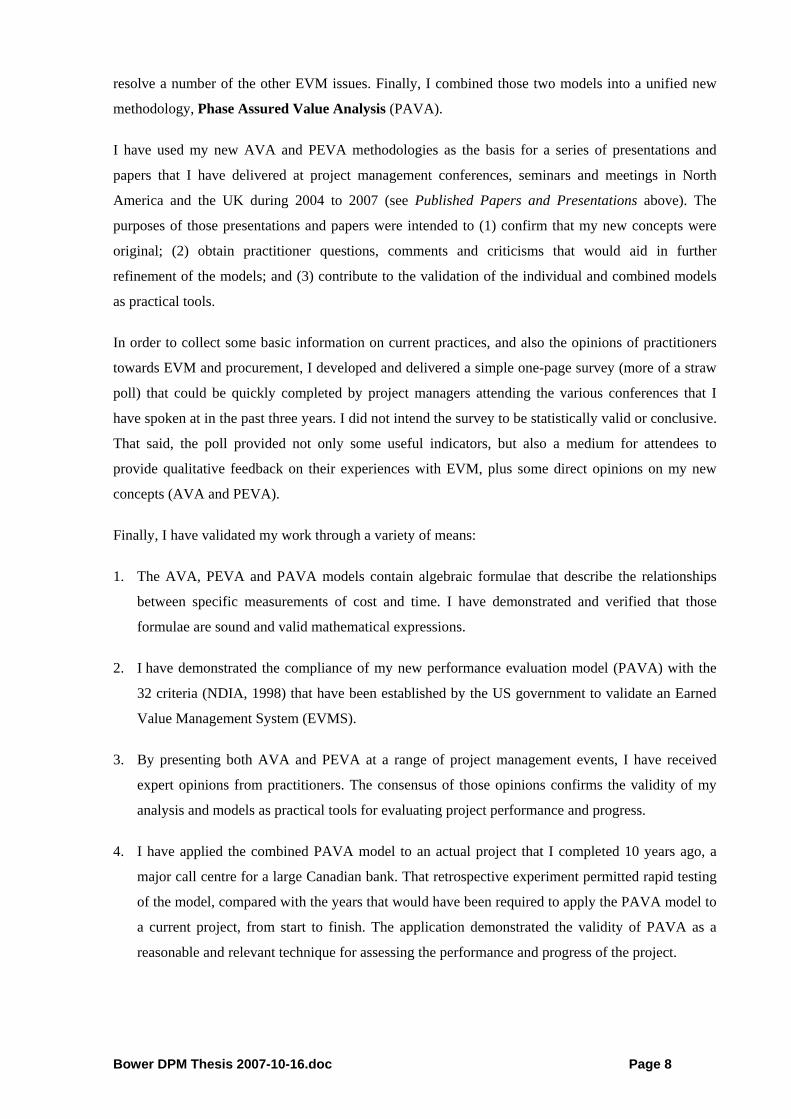
Finally, I have validated my work through a variety of means:

1. The AVA, PEVA and PAVA models contain algebraic formulae that describe the relationships

between specific measurements of cost and time. I have demonstrated and verified that those

formulae are sound and valid mathematical expressions.

2. I have demonstrated the compliance of my new performance evaluation model (PAVA) with the

32 criteria (NDIA, 1998) that have been established by the US government to validate an Earned

Value Management System (EVMS).

3. By presenting both AVA and PEVA at a range of project management events, I have received

expert opinions from practitioners. The consensus of those opinions confirms the validity of my

analysis and models as practical tools for evaluating project performance and progress.

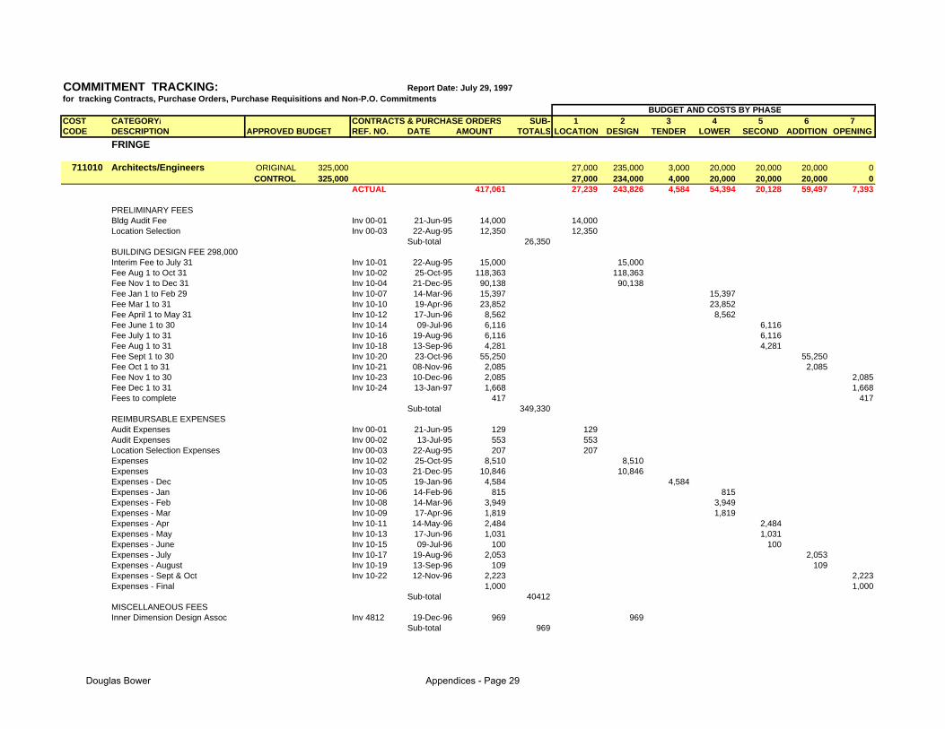
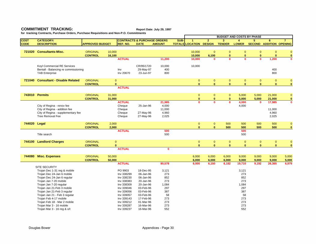
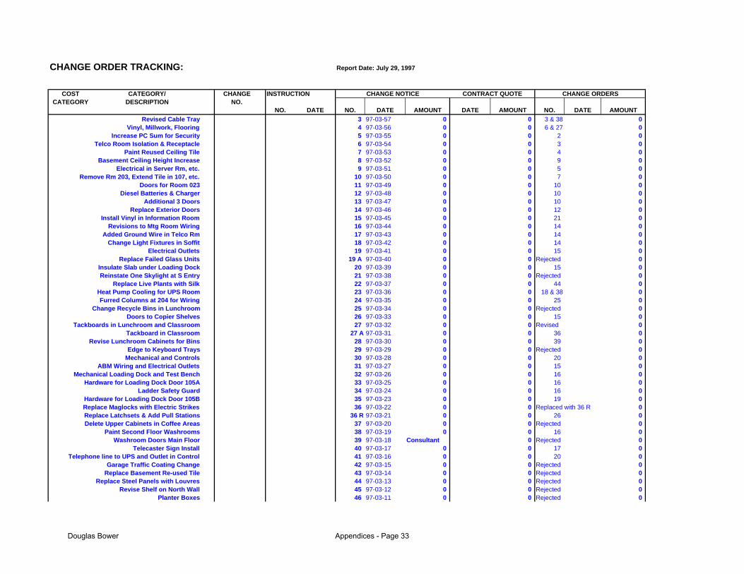
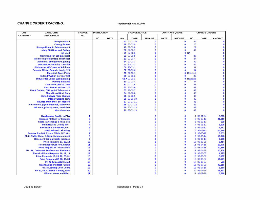
4. I have applied the combined PAVA model to an actual project that I completed 10 years ago, a

major call centre for a large Canadian bank. That retrospective experiment permitted rapid testing

of the model, compared with the years that would have been required to apply the PAVA model to

a current project, from start to finish. The application demonstrated the validity of PAVA as a

reasonable and relevant technique for assessing the performance and progress of the project.


1.6 DPM Research Program

I was attracted to the Doctor of Project Management program as it provided a flexible but rigorous

academic environment in which I could develop ideas, concepts and models that would address some

of the questions related to project management – such as the paradox of EVM being high in value, but

low in usage. The program design facilitates not only the discipline that is necessary for performing

doctoral level research, but also the collaboration that is possible within the community of practice that

is formed by two dozen project management practitioners, some with decades of varied experience.

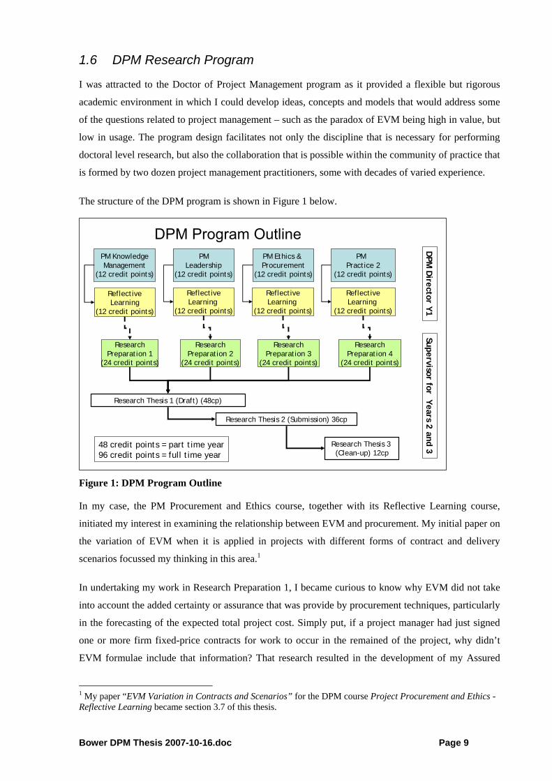
The structure of the DPM program is shown in Figure 1 below.

ReflectiveLearning

(12 credit points)

DPM Program OutlinePM KnowledgeManagement

(12 credit points)

ResearchPreparation 1

(24 credit points)

Research Thesis 1 (Draft) (48cp)

Research Thesis 2 (Submission) 36cp

ReflectiveLearning

(12 credit points)


(24 credit points)

PMLeadership

(12 credit points)

ReflectiveLearning

(12 credit points)


(24 credit points)

PM Ethics & Procurement

(12 credit points)

ReflectiveLearning

(12 credit points)


(24 credit points)

PM Practice 2

(12 credit points)

Research Thesis 3 (Clean-up) 12cp

DPM

Director Y1

Supervisor for Years 2 and 348 credit points = part time year96 credit points = full time year

Figure 1: DPM Program Outline

In my case, the PM Procurement and Ethics course, together with its Reflective Learning course,

initiated my interest in examining the relationship between EVM and procurement. My initial paper on

the variation of EVM when it is applied in projects with different forms of contract and delivery

scenarios focussed my thinking in this area.1

In undertaking my work in Research Preparation 1, I became curious to know why EVM did not take

into account the added certainty or assurance that was provide by procurement techniques, particularly

in the forecasting of the expected total project cost. Simply put, if a project manager had just signed

one or more firm fixed-price contracts for work to occur in the remained of the project, why didn’t

EVM formulae include that information? That research resulted in the development of my Assured

1 My paper “EVM Variation in Contracts and Scenarios” for the DPM course Project Procurement and Ethics - Reflective Learning became section 3.7 of this thesis.


Value Analysis (AVA) model, and I presented the resulting paper at two project management

conferences at the end of 2004.2

Similarly, while proceeding with Research Preparation 2, I returned to my interest in project phases to

question why EVM methodology disregarded phases in any of its concepts and calculations. That line

of inquiry led to the development of my Phase Earned Value Analysis Concept, which I presented at

several major conferences in 2005 and 2006.3

This progression of research and inquiry that I experienced is well illustrated in Figure 2: DPM

Program Contribution below, which represents the progression that a DPM candidate may experience

in the program. I began in the lower left quadrant (Q1) studying the ‘as is’ situation regarding project

procurement, phases and performance evaluation. During the program I moved to Q2 in proposing

new concepts and techniques that ‘could or should’ be utilised. From there I continued to Q4 in

developing new approaches to evaluating the progress and performance of a project, specifically the

new models for AVA and PEVA.

New

Con

cept

/Too

l/Pe

rfor

man

ce m

easu

rem

ent a

gent

s

New Application/Geographical AreaLow High

High

Auditing ‘as is’ Situation analysisMapping/plottingReflection

Proposing ‘could or should be’ Modifying + trial & error, action learning

Modifying, studying new context influences and refining, action learning

Developing new systems, new approaches, new tools

Q1

Q2

Q3

Q4Knowledge

Management

PM Leadership

PM Procurement

+ Ethics

PM Practice 2

DPM Program Contribution

Figure 2: DPM Program Contribution

1.7 Chapter Summary and Thesis Structure

This chapter introduced the topic of my thesis in the context of project management knowledge, and

acknowledged some of the limitations of this thesis. I identified how my research adds value to the

body of project management knowledge. I have identified the research problem, and the key questions

2 PMI Global Congress 2004 in Anaheim, CA and the IPMC Conference 2004 in Washington, DC, USA 3 PMI Global Congress 2005 in Toronto; the BPPM Summit 2006 in London, UK, the PMI Research Conference 2006 in Montreal; and the CPM 22nd International Conference, Clearwater Beach, Florida.


associated with it. I have also described my professional and academic background, and how the

Doctor of Project Management (DPM) program not only acted as a catalyst for organising and

advancing my research into the topic of project performance evaluation in general, and EVM in

particular.

The thesis is organised into Chapters for ease of reference, and a brief description of each is provided

here.

1. Introduction and Justification: The purpose and context of research are described, and the

research questions and propositions are outlined.

2. The Supporting Literature: The bodies of knowledge addressed here include project types, scope

management, project controls, risk management and stakeholder engagement.

3. The EVM Approach: This covers the origins, basis and theory of EVM, its adoption and standards,

and conventional EVM methodology. Time management and earned value is explored, particularly in

relation to Earned Schedule (a new extension to EVM) and to project phases. EVM variation in project

contracts and delivery scenarios is analysed here, in order to recognise the various contexts in which

EVM can be applied. EVM is also compared to procurement and risk management practices. From this

review and analysis, a series of research issues are confirmed and described.

4. Research Design: Based on this review of EVM in relation to project context situations,

procurement practices, risk management and scheduling, I developed a research plan that has been

implemented in the course of this doctoral program. That research plan includes the following key

elements:

• a review of previous and current literature on EVM and closely related topics;

• surveying PM practitioners on their project control practices and attitudes towards EVM;

• analysis of the known challenges (gaps, anomalies, weaknesses) of EVM techniques;

• development of new conceptual techniques to address and resolve those EVM challenges;

• consolidation of those techniques into a single framework and implementation model; and

• validation of that framework and model through multiple methods.

5. Hypothesis and Model Development: In this chapter, I describe two new concepts that I have

developed in the course of the DPM program, and which I have introduced at various PM conferences

over the past three years. I developed Assured Value Analysis to recognise the effects of procurement

in project performance evaluation and forecasting – something that EVM does not do. I developed

Phase Earned Value Analysis to address the other shortcomings of EVM, such as its inability to

chart trend lines for forecast AC and EV values beyond the date of earned value review. Both new


concepts resulted in new measures, and in expanded formulae; those are incorporated into spreadsheet

models that are demonstrated in this chapter with notional projects. I combined both AVA and PEVA

into a single model (PAVA), which I also demonstrated with a simplified sample project. I also

demonstrate how the PAVA indicators, being phase-based, provide a very useful foundation for

visualising the status of projects and programme in comprehensive portfolio management.

6. Analysis and Discussion: I have validated the combined model through multiple techniques.

• Mathematical and deductive reasoning has been applied to confirm the validity of the new

measures (AV, EC, etc.), the enhanced formulae, and the comprehensive models.

• Comparison to EVM standards was undertaken to confirm that the combined approach

(PEVA with AVA) complies with the 32 criteria contained in the established global EVM

standard.

• Actual project implementation was successfully applied retrospectively to a large project

that I managed in the last decade, for which I possessed all relevant cost and schedule

information.

• Practitioner validation was obtained from project managers and academics that attended

my conference presentations or participated in seminars that I delivered on AVA and

PEVA. That feedback was provided in two main channels: comments written on the

survey forms that I provided to attendees, and specific questions that attendees posed

during those presentations.

7. Conclusions: I provide my conclusions to the research studies that are contained within this thesis.

I revisit the research problem and questions posed at the beginning of Chapter 1, and provide

responses with the benefit of the intervening research and analysis. I reiterate the significant

shortcomings that have slowed EVM adoption in many industries and project types, and explained

how PAVA not only addresses those shortcomings, but also provides additional benefits. The value

added by these new extensions to EVM is identified, plus implications for PM practice. Finally, I

identify directions for further research.

8. References: Thesis bibliography.

9. Glossary: Definition of EVM and related terms used in this thesis.

Appendices A-E: Additional detailed information on aspects of the thesis topic and research.


2 The Supporting Literature In this chapter I make reference to the supporting literature on a range of project management topics

that are directly related to project performance evaluation and EVM. The literature is mainly from

academic sources, but also includes some expert practitioner contributions. Those are particularly

important given my desire to ensure that my development of this topic is not only theoretically valid,

but also relevant to active managers and directors of projects and programmes.

I address project types and their influence on the need for project control methodologies such as EVM.

I review project uncertainty and risk management. Finally, I review the role of project stakeholders,

and the potential of EVM as a tool for communication and engagement of many stakeholder groups.

2.1 Project Types

At one time, a clear distinction may have existed between organisational operations and projects;

however, the past decade has seen a significant projectification or widening of the definition of

projects and project management. (Maylor, Brady, Cooke-Davies, & Hodgson, 2006)

The PM bodies of knowledge have defined a project as “a temporary endeavour undertaken to create a

unique produce, service or result” (PMI, 2004, p. 368) and “unique, transient endeavours undertaken

to achieve a desired outcome” (APM, 2006). Both definitions are broad, and perhaps vague.

Kerzner has defined a project (2003, p. 2) more specifically, as “any series of activities and tasks that

(1) have a specific objective to be completed within certain specifications, (2) have defined start and

end dates, (3) have funding limits (if applicable), (4) consume human and non-human resources, and

(5) are multi-functional (i.e. cut across several functional lines).” This definition typifies a traditional

recognition of projects as the means to create physically large and technically complex deliverables

within multi-faceted organisations. However, Kerzner appears to be unnecessarily prescriptive. For

example: some projects have vague objectives or lack defined end dates; many do consume only

human resources; others are delivered by just one functional group. So, these five stipulations may be

useful in forming an image of a typical project, but tend to eliminate many valid projects that do not fit

the mould.

Turner (1999, p. 3) defines a project as “an endeavour in which human material and financial

resources are organised in a novel way, to undertake a unique scope of work of given specification,

within constraints of cost and time, so as to achieve unitary, beneficial change, through the delivery of

quantitative and qualitative objectives.”

Projects have a purpose, a life cycle, interdependencies, uniqueness and conflicts (Meredith & Mantel,

2003, p. 9). Those five characteristics respectively lead to: dedicating resources for their completion,


time schedules for their organisation, relationships between their components, responses to their

uncertainty and the communication between their stakeholders. I will examine all of those items in

this thesis, through the lens of project performance management.

Many researchers and authors have attempted to classify projects by certain characteristics. Kerzner

(2003, p. 23) suggests that they be classified by industry, namely: In-house R&D, Small Construction,

Large Construction, Aerospace/Defence, MIS, and Engineering. He advises that project management

principles may be applied to any project, but the importance of those PM principles will vary from one

industry to another. Kerzner observes that in project-driven industries (such as aerospace and large

construction) the large investment mandates a much more rigorous PM approach. This perspective is

not surprising, as his text is subtitled a systems approach to planning, scheduling and controlling.

Turner and Cochrane (1993) advocate judging projects against two parameters: how well defined are

the goals, and how well defined are the methods for achieving them. This leads to four types of

projects: (1) Goals and methods of achieving the project are well defined; (2) Goals are well defined,

but the methods are not; (3) Goals are not well defined, but the methods are; and (4) Neither the goals

nor the methods are well defined.

Type 1 Project“Earth”

Engineering

Type 2 Project“Water”Product

Development

Type 4 Project“Air”

Research & Organisational

Change

Type 3 Project“Fire”

Applications Software Development

Greater chance

of failure

Greater chance

of success

Goals Well Defined

Methods Well Defined

Yes

No

Goals and Methods Matrix

Source: Turner & Cochrane (1993)

Yes No

Figure 3: Goals and Methods Matrix

These four types are illustrated in Figure 3 above. The authors have named each quadrant after the

four traditional elements (earth, water, fire, air) and have provided a typical project as an example.

Turner and Cochrane (1993) outline both startup and implementation techniques appropriate for these

four project types. They also advise that three breakdown structures are relevant here: the Product

Breakdown Structure (PBS) to define the deliverables, the Organisational Breakdown Structure (OBS)

to identify resource types, and the Work Breakdown Structure (WBS) which is a two-dimensional


matrix of products and activities. With this perspective, Turner and Cochrane (1993, p. 98) argue that

“only on Type -1 projects is it possible to plan the project in terms of the activities to be undertaken”.

On the other project types, the WBS is ill-defined, to varying degrees. Since the WBS is a prerequisite

for the application of EVM, this implies great difficulty in using EVM for projects that fall into

quadrants 2, 3 and 4 of the Goals and Methods Matrix. For those types, Turner and Cochrane further

recommend the use of milestone planning, in which the plan is expressed in terms of control points or

milestones. For Type 2 projects, they suggest that the needed methods and tasks be planned on a

rolling-wave basis. For Types 3 and 4, the milestones must instead be decision points where the

definition of the goals is refined.

At this point, I must observe that project phases provide an ideal means for establishing milestones and

control points, and also for organising the rolling-wave planning. Phase stage gates also provide

convenient decision points for goal definition. I return to this notion later in this thesis.

Shenhar (2001) used case studies to explore a wide spectrum of technical projects, then suggest a

conceptual framework for the classification of projects, then proceed towards that development of a

typological theory of projects. The conceptual model used two main dimensions, each subdivided into

several levels. Technological uncertainty formed four levels: Low-Tech, Medium-Tech, High-Tech,

and Super High-Tech. System scope was divided into three levels: Assembly, System and Array.

Technological Uncertainty

Typology of Technical ProjectsSource: A. Shenhar (2001)

Contingency mgmt.

BMedium-

Tech

ALow-Tech

CHigh-Tech

DSuper

High-Tech

System Scope

1Assembly

2System

3Array

Size, Planning, Control,

Subcontracting, Bureaucracy,

Documentation, Computerization

Systems engineering, System

integration, Configuration mgmt,

Risk mgmt.

Development & testing, Late design freeze, Technical skills, Flexibility, Communication, Risk, Opportunity

Contingent Relationships

Figure 4: Typology of Technical Projects

Those dimensions and levels are illustrated above in Figure 4, along with contingent relationships that

Shenhar argued are relevant along the dimensions of uncertainty and scope.

Shenhar also identified variables according to those two dimensions, and examined the project

characteristics evident for each of the dimension levels. He found that an important variable for system


scope was “control and reports”, and noted (Shenhar, 2001, p. 254) that control became both more

formal and more complex for projects with a higher scope level. An Assembly project needs only

“simple, in-house control” with all “reporting to management or a major contractor”. A System project

requires “tight and formal control on technical, financial and schedule matters”. Finally, an Array

project demands “master or central control of program with separate additional control mechanisms”.

He observed that some of the case studies were considered System projects, and several utilised highly

formal control and reporting methodologies, including EVM. Array level initiatives, however, were

often treated as programs, with the control and reporting devised separately for each sub-project.

Performance management – and specifically conventional EVM – appears most relevant to System

and Array projects (as classified by Shenhar) and that has been borne out by the origins of EVM and

its adoption patterns, particularly in the USA. It appears (Christensen, 1998) that the considerable

costs of implementing EVM can be justified only in projects that are highly technical and complex,

such as weapons systems. In this thesis, I have addressed means of simplifying earned value

techniques, in order to make it less costly on assembly and other straightforward projects – but at the

same time providing additional features, so as to increase its benefit to organisations.

There appears to be an increasing occurrence of projects with intangible results and diffuse outcomes –

ones that address on change management (such as corporate mergers), or social benefit (e.g. aid

projects). In these less-focussed projects, success may be defined more by the perception that they

have met their goals and achieved stakeholder satisfaction – rather than being delivered on time and on

budget (Smith, 2007).

2.2 Project Control

As defined by the PMBOK Guide (PMI, 2004) there are five essential project management processes,

namely: Initiating, Planning, Executing, Controlling and Closing.

Controlling is a combination of two elements: monitoring and taking corrective action. PMBOK

defines control as “comparing actual performance with planned performance, analysing variances,

assessing trends to effect process improvements, evaluating possible alternatives, and recommending

appropriate corrective action as needed.” (PMI, 2004, p. 355) A comparison of this definition with the

description of Earned Value Methodology in section 3.5 below indicates that EVM should be essential

(at least, according to PMI) for the proper control of most projects. This definition of control could

also be applied to quality management and to human resource management, by assigning different

meanings to terms such as performance (e.g. staff performance) and variance (e.g. quality variance).

The Gantt chart was one of the earliest management tools devised for the planning and control of

projects. Some researchers are looking beyond the Gantt chart (Maylor, 2001) and other conventional

techniques, towards other approaches to strategy, planning and assessment for projects that exist


beyond the traditional definition. Maylor (2001, p. 99) recommends better integration of project

performance and business drivers, and specifically concludes that “project performance management

clearly needs development in the light of the move from conformance-based measures and the

popularity of approaches such as the balanced scorecard”. Certainly a new approach such as the

balanced scorecard (Kaplan & Norton, 1992) provides an important perspective for viewing the

performance of the organisation and its broad outcomes; however, that technique does not negate the

value of assessing the performance of individual projects, through either conventional EVM or new

variants and extensions of it.

The element of project management were visualised (Forsberg, Mooz, & Cotterman, 1996) in tabular

form with the rationale and major focus for each element, as reproduced in Table 1 below. Project

control, visibility, status and corrective action are identified as key elements, and I suggest that those

are directly linked to project performance evaluation, which has been conventionally performed

through EVM.

Table 1: Elements of Project Management

Elements of Management

Rationale Major Focus

Requirements Failure to manage requirements which initiate and drive projects is the major cause of failure.

Formulate

Organizing Putting structure around the key activities, people, and resources is critical to successful management.

Project Team Teams are newly formed for each project and include subcontractors and outsourcing.

Planning Needed to overlap roadmap of tasks to be done including schedule, budget, and deliverables.

Proactive

Risk and Opportunity Management

Significant cause of project failures if not specifically managed.

Project Control When properly implemented, controls identify whether project is proceeding appropriately.

Visibility Needed to keep all stakeholders informed.

Status Need hard metrics, measures, and variances to supplement activity reports.

Variance Control

Corrective Action Innovative plans needed to get back on track with plan. Reactive

Leadership Creation of team energy to succeed with plan. Motivate

Source: Visualizing Project Management (Forsberg, Mooz, & Cotterman, 1996)

Effective project management requires project control mechanisms (devices, structures, events) that

can track progress and performance as the project proceeds. Those mechanisms can produce output

reports that inform stakeholders and reinforce visibility. The hard metrics, measures and variances

compare the project’s performance and progress against the plan and provide the needed alerts to spur

corrective action as needed. (Pearlson & Saunders, 2004, p. 252)


The selection of a project control system is an important element in the management of a project or

program (Shtub, Bard, & Globerson, 2005) and the lack of such systems has been identified with a

major role as a cause of project failures. (De Falco & Macchiaroli, 1998)

Project control systems can be classified as either one-dimensional or multi-dimensional according to

an extensive review (Rozenes, Vitner, & Spraggett, 2006) of current literature on this subject. Both

types include one or more predefined project control objectives, such as cost, time, quality, etc. In one-

dimensional control systems, those objectives are not integrated in any way; however, in multi-

dimensional systems several objectives are integrated. EVM is the most commonly used

multidimensional project control method, as it integrates time and cost. Other types deal with risk

management, statistical process control, etc. The authors conclude that a key disadvantage of EVM is

that other project control dimensions – quality, design, technology, etc. – are not integrated into it.

They suggest that more research is needed to integrate additional control dimensions into the EVM

approach.

With either a one-dimensional or two-dimensional control system, an important factor is determining

the best times to perform the control activity. One study (Raz & Erel, 2000) proposed an analytical

framework for determining the optimal timing of project control points throughout the life cycle of the

project.

Meyer (1994, p. 96) suggests that “trying to run a team without a good, simple guidance system is like

trying to drive a car without a dashboard”. He suggests the following four guiding principles for

overhauling performance measurement systems to maximize team effectiveness:

1. A measurement system should allow the team to gauge its progress.

2. The team should play a lead role in designing its own measurement system.

3. Because a team is responsible for a value-delivery process that cuts across several

functions… it must create measures to track that progress.

4. A team should adopt only a handful of measures, based on what gets measured gets done.

EVM was developed by the US Department of Defense (DoD) as a project control system that

specifically integrated the time and cost dimensions. (Abba, 1997) A work breakdown structure

(WBS) is used to provide the integration necessary between these two very different dimensions. A

WBS requires the hierarchic structuring of the project using its major components and subcomponents.

The lowest level of the WBS is the work package, which comprises a set of related tasks to be

performed by a single organisational unit (PMI, 2001). Some attention has been paid to determining

the optimum size of such work packages (Raz & Globerson, 1998) in order to maximize benefits while

minimizing the necessary administrative effort.


2.3 Project Phases and Scheduling

A project phase is defined in PMBOK as a “collection of logically related project activities, usually

culminating in the completion of a major deliverable. Project phases (also called phases) are mainly

completed sequentially, but can overlap in some project situations. Phases can be subdivided into

subphases and then components; this hierarchy, if the project or portions of the project are divided into

phases, is contained in the work breakdown structure. A project phase is a component of a project life

cycle. A project phase is not a project management process group.” (PMI, 2004, p. 369)

Also, from a British perspective: “Project life cycles consist of a number of distinct phases. All

projects follow a life cycle and life cycles will differ across industries and business sectors. A life

cycle allows the project to be considered as a sequence of phases which provides the structure and

approach for progressively delivering the required outputs.” (APM, 2006)

On information technology (IT) projects, a systems development life cycle (SDLC) has been

recognised as a useful model for breaking down the scope and major stages of software application

development. The SDLC consists of several distinct phases that are followed methodically: Planning,

Analysis, Design, Implementation and Support (Oz, 2002, p. 579). Variations on the SDLC are

available. For example, the Staged Implementation Model (S. C. McConnell, 2002) specifically

addresses requirements volatility, risk assessment, scheduling difficulties, and product concurrency by

developing the product in seven stages.

Jalotte et al (2003) describe an iterative software development approach that allows the functionality

to be delivered in parts, as an effective way to manage risks. They propose the timeboxing model for

iterative software development in which each iteration is done in a time box of fixed duration, and the

functionality to be built is adjusted so that it will fit the time box. The authors suggest that by dividing

the time box into stages, pipelining concepts can be employed so that multiple time boxes execute

concurrently, leading to a reduction in the delivery time for product releases.

WBS and Phases

It is important to recognise that a project manager will typically use the phases of a project as the

primary divisions in its WBS. According to the PMI Practice Standard for WBS, the upper levels

“typically reflect the major deliverable work areas of the project or phases in the project’s life cycle.

These levels also provide logical summary points for assessing performance accomplishments, as well

as measuring cost and schedule performance.” (PMI, 2001, p. 4) PMI’s connection between project

phases and the WBS upper level is highly relevant to my thesis, even though I will later point out that

project performance measurement does not necessarily require the use of a WBS common to both cost

and time dimensions.


Risk management activities and risk exposures (both threats and opportunities) vary considerably over

the duration of a project. Project phases represent a natural and convenient framework for identifying

new risks, retiring previous no-show risks, directing risk response techniques, assessing the status of

risk exposures and documenting lessons learned. “The actual content of the risk analysis and risk

management appears to differ depending on the [current] phase of the project and the phase being

targeted.” (van Well-Stam, Lindenaar, van Kinderen, & van den Bunt, 2004, p. 83)

In the development of new products, a phased approach can lead to improved understanding, a greater

sense of urgency, and reduced risk. (Rosenau, 1993, p. 409)

Rolling-Wave Approach

With this approach to project management, fully detailed activity plans are developed only for work

packages that are about to begin in the short term (J.R. Turner, 1999, p. 114). When using EVM, this

means that the project budget (especially on projects of long duration or high uncertainty) is composed

of two types of approved cost estimates: detailed cost figures for current and approaching work

packages, and high-level cost figures for undefined future work packages. It is important to the

integrity of EVM systems that the budgets for those long-term planning packages be strictly separated

from those for current and upcoming detailed work packages. (Fleming & Koppelman, 2005, p. 199)

Rolling wave is also important as it addresses a contradiction in standard EVM. That is, EVM is

particularly useful for complex projects with a high degree of uncertainty, such as weapons systems

(hence the DoD interest). However, EVM also requires an S-curve baseline at the outset, which means

an approved budget for the whole project. How can one do that when project scope is so ill-defined?

The rolling wave permits detailed budgets to be adopted for upcoming work, and high-level budgets to

be assigned to later control accounts. I note here that my PEVA model will facilitate both as budgets

can be prepared and approved by phases: detailed for early phases, rough for later ones.

Kill points

Schulyer (2001, p. 77) points out that research projects often have a series of formal gateways or

points at which the project may be stopped. As an example, the process for creating a successful new

drug, from conception to market, goes through a series of stages of development, testing and approval.

“Each milestone is a decision point, primarily to continue or drop.” Schulyer confirms that some

research projects will never reach the customer. “When necessary, let’s hope that the project ‘kill’

decision is deliberate and made in time. New information during the project helps us to determine

when dramatic intervention may be necessary.” (Schuyler, 2001, p. 77)


Critical Path and Critical Chain

Conventional EVM provides very limited techniques for assessing project schedule progress and for

forecasting the project completion date. In addition, those techniques have been found to be

significantly flawed, as described in section 3.6. Even the most ardent supporter of EVM will caution

that the schedule progress facet of EVM should be used only as an early warning system. Clearly, the

best method for determining schedule status and the expected completion date is a properly maintained

network or Gantt chart using the Critical Path Method (CPM), on which the project manager records

not only the planned start/finish dates for activities, but also their actual start/finish dates.

The CPM is “a schedule network analysis technique used to determine the scheduling flexibility (the

amount of float) on various network paths in the project schedule network, and to determine the

minimum total project duration.” (PMI, 2004, p. 357) It should be clear that if a project is organised in

a single set of sequential phases, the Critical Path must flow through each of those phases. In addition,

even though the Critical Path will not flow through every activity and milestone in that phase, it must

flow through the final milestone that represents completion of that phase. If a project has several sets

of sequential phases forming a network, then the critical path will not necessarily pass through every

phase, but will pass through the sequence of phases that determines the minimum total project

duration.

The preparation of any project schedule necessarily requires the team to estimate the duration of

project activities, and frequently such estimates are based on incomplete information. The durations

entered in a CPM schedule are therefore approximations of the expected duration, with the expectation

that the actual duration may be slightly shorter – or considerably longer. As a longer duration is more

likely and more problematic than a shorter one, it is quite understandable for team leads to ‘pad’ their

duration estimates so that there is reduced chance of having insufficient time, particularly in the event

of unexpected delays or complications. Goldratt (1997) has observed this phenomenon and proposed

the Critical Chain technique, in which those individual hidden periods or ‘buffers’ are pooled to

create an explicit project buffer that is placed at the end of the schedule. Also, a feeding buffer may be

placed at the end of a non-critical group of activities, so that they do not become part of the critical

path, should they become delayed. Finally, a resource buffer may be created as a virtual task prior to

critical chain tasks that require critical resources.

Initially, some authors tended to support Critical Chain (Leach, 1999). A recent critique of Critical

Chain has concluded that although it presents a number of valuable concepts, “it does not provide a

complete solution to project management needs, and that organisations should be very careful about

the exclusion of conventional project management techniques” (Raz, Barnes, & Dvir, 2003, p. 24).

Although this thesis does not specifically support it, Critical Chain appears compatible to the notions

of recognising the significance of project phases, and assessing performance on phase completion.


2.4 Project Uncertainty, Risk Management and EVM

All projects include varying degrees of uncertainty. Ward and Chapman (2003, p. 97) suggest that

project risk management (PRM) processes as currently advocated in PM texts and bodies of

knowledge have a “limited focus which restricts the contribution to improving project management

practice and hence project performance.” They believe that limited focus is in part because the term

risk encourages a threat perspective, and in part because PRM has become associated with events

rather than more general sources of significant uncertainty. Ward and Chapman recommend the term

uncertainty management rather than risk management, as a first step towards dealing with both of

those concerns.

Historically risk events have been seen as mainly negative occurrences, and many project management

texts treat risk in that manner. More recently, risk events have been recognised to be either positive or

negative in their impact on a project. Positive events are termed opportunities, and their recognition is

found in the 3rd edition of the PMI Body of Knowledge (2004) and other risk literature (Hillson,

2004b). That said, the term risk in common usage normally has negative connotations, and therefore it

is difficult in practice to become accustomed to perceiving risk management as embracing events with

either positive or negative outcomes.

However, Ward and Chapman (2003) go beyond semantics. They suggest that adopting uncertainty

management leads to the recognition of a broader scope of uncertainly, beyond identifying potential

risk events. They argue that uncertainty exists in five areas: the variability associated with estimates of

project parameters; the basis of estimates of project parameters; design and logistics; objectives and

priorities; and relationships between project parties.

EVM also addresses uncertainty, particularly the uncertainty surrounding time and cost performance.

The use of EVM measures, variances and indicators provides management with useful advance

warnings as to the degree of risk that time and cost objectives will be met. It can also identify sources

of past performance successes and difficulties, by calculating indices and variances on the

performance of specific groups (vendors, departments, etc.) or types of activities (e.g. control

accounts, work packages).

Despite these obvious links with earned value methodology, most recent books and papers on risk

management do not address EVM directly; however, some do refer to project management techniques

that are shared by both EVM and PRM. For example, in Megaprojects and Risk, Flyvbjerg et al (2003,

p. 141) state that “both staff and directors must be conversant with the implications of performance

management and the notions of risk and accountability.” Project performance management is can be

delivered through EVM, but that is not mentioned.


Project risk management standards (PMI, 2004) and texts (Hillson, 2004b, p. 39; Royer, 2002, p. 35;

van Well-Stam, Lindenaar, van Kinderen, & van den Bunt, 2004, p. 51; Wideman, 1992) generally

identify four categories of responses dealing with negative risk: acceptance, avoidance,

mitigation/reduction and transfer. The two main tactics for transferring risk are either through the use

of financial instruments (insurance, bonds, etc.) or through the procurement of goods and services at

assured prices from suppliers such as consultants and vendors. This establishes an important link

between risk management and procurement management. It is also clear that since procurement

arrangements (contracts, agreements, purchase orders, etc.) are made in advance of the work to be

performed, those could represent an important factor in any cost re-estimating work that may take

place during the course of the project. Such re-estimating occurs both manually and by formula in

EVM. That relationship is revisited in sections 3.8 on Procurement and 5.3, which deals with my

Assured Value Analysis concept.

An important strength of EVM lies in its rigorous examination of what has already occurred on a

project. One of the perceived weaknesses of EVM is its reliance on a key assumption, that future

performance can be predicted from past performance patterns. By comparison, project risk

management (PRM) identifies potential future risks and benefits, together with their probability of

occurrence, and uses that information to assess the range of project outcomes. This important strength

of RM is also one of its key weaknesses. Events which have already taken place are not relevant to the

risk processes, since there is no uncertainty associated with them. Hillson (2004a) proposed that “a

useful synergy might be obtained if a combined EVM-RM approach were able to address these

weaknesses.”

It is worth noting at this point that most project management techniques, such as Gantt charts, Critical

Path Method (CPM) calculations, and even Program Evaluation and Review Technique (PERT) are

deterministic project models. EVM is also deterministic, as it produces a single forecast of future cost

and schedule outcomes based on past performance and progress. Risk techniques such as Monte Carlo

analysis are stochastic, or probabilistic, forecasts as they take into account probability distributions of

unknown values for key variables. (Schuyler, 2001, p. 121)

Hillson noted that the EVM performance measurement baseline is typically seen as an S-shaped curve

beginning at zero and increasing over the planned project duration to the budget at completion (BAC).

He suggested that undertaking a full risk assessment (using a stochastic approach) at or soon after

project inception would result in the recognition of both best and worst case project outcomes, plus all

other possible outcomes between those extremes. Those can be shown as a set of three related S-curves

representing the best case, most likely case, and worst case scenarios. This is shown in Figure 5 below.

Although these are typically referred to as curves the lines representing these three sets of outcomes

would not usually be symmetrical and smooth lines as shown in the figure. It would be possible to


calculate the data points on each of these three curves as the risk simulation software can produce a

range of possible results for regular intervals on the time scale.

Using Risk Analysis to Plot the PMB

Time Schedule

Proj

ect V

alue

and

Cos

t

Use this as PMB

Best Case:Minimum Cost and

Earliest Time

Worst Case:Maximum Cost and Latest Time

EARLIEST PROJECT

END

LATEST PROJECT END

EXPECTED PROJECT

END

EXPECTED TOTAL COST

MINIMUM TOTAL COST

MAXIMUM TOTAL COST

Individual Time/Cost

Results

Source: Hilson (2004) EVM and Risk Management: A Practical Synergy

BAC

Figure 5: Using Risk Analysis to Plot the PMB

Hillson further proposed that EVM and PRM could be combined during the project execution, through

an EAC formula that would include not only the CPI (or a performance efficiency factor based on both

CPI and SPI) but also the known risks and unknown uncertainty on the remainder of the project. The

result would be a collection of individual time/cost results that would cluster as shown in Figure 6

below.


Using Risk Analysis to Plot the EAC

Time Schedule

Proj

ect V

alue

and

Cos

t Worst Case:Maximum Cost and Latest Time

EARLIEST PROJECT

END

LATEST PROJECT END

EXPECTED PROJECT

END

EXPECTED TOTAL COST

MINIMUM TOTAL COST

MAXIMUM TOTAL COST

Source: Hilson (2004) EVM and Risk Management: A Practical Synergy

Best Case:Minimum Cost

and Earliest Time

Use this as EAC

ACTUAL COST TO DATE

TIME NOW

NOTE: EARNED VALUE AND PLANNED VALUE CURVES TO DATE ARE NOT SHOWN

Individual Time/Cost

Results

Figure 6: Using Risk Analysis to Plot the EAC

The worst case results would indicate the maximum total cost and latest project end date; the best case

results would indicate the minimum total cost and earliest project end date. The central point on the

line joining those two extremes represents the estimated total cost, also known as the Estimate at

Completion (EAC).

Hillson’s combined PRM-EVM approach represents a valuable contribution to project performance

evaluation, and certainly an area of research that deserves greater attention. His approach should be of

particular interest to researchers that wish to test out improvements to EAC formulae, which are

outlined later in this thesis.

I have not pursued Hillson’s combined approach in this thesis, as it appeared to be adequately

theorized and described. Further, I wished to determine how to simplify EVM processes and also to

provide additional features, both with the objective of increasing the adoption of earned value

techniques by project management practitioners. Combining risk management with EVM has its

merits, but certainly does not simplify the evaluation process.

For example, although it is possible to plot a time-phased budget, known as the Performance

Management Baseline (PMB), on a chart as shown in Figure 5: Using Risk Analysis to Plot the PMB,

it would be very demanding to plot the expected future actual costs as shown in Figure 6: Using Risk

Analysis to Plot the EAC. That is because the expected dates and budget amounts for future work

packages are contained in the project plan, but the expected dates and actual costs for future work are


not known. Risk techniques (such as Monte Carlo analysis) should be able to generate the required

data to plot the Actual Cost line, but doing so would be rather challenging for many practitioners.

2.5 Chapter Summary

The definition of projects and classification of project types is highly germane to this thesis. While the

definitions found in project management bodies of knowledge are so broad that they encompass all

possible temporary endeavours, other sources have defined projects more closely to those initiatives

traditionally found in the industries where project management was first developed – construction,

aerospace, and the military. However defined, projects possess uncertainty, and that feature is

important to any discussion of project performance measurement.

Some have attempted to classify projects according to their characteristics, such as their industry

sector. That makes some sense; it is already clear that performance measurement, using EVM, initiated

within specific industries, such as those associated with military systems.

Turner and Cochrane advocate assessing projects according to the clarity of their goals and objectives.

Managers wishing to implement project performance measurement require some specifics around

goals and objectives, so that the necessary cost estimating and activity planning can be performed as a

necessary prerequisite to finalising a budget and time schedule. Conventional EVM is best suited to

projects with highly defined goals and methods, as that will facilitate creating the Work Breakdown

Structure (WBS) and plotting the Performance Measurement Baseline (PMB). Projects that lack well-

defined goals or objectives appear to be unsuited to conventional EVM. However, the need to establish

milestone planning on these less-defined projects leads me to recommend the use of phases as a means

to both identify those milestones, and also a framework for performance measurement – my Phase

Earned Value Analysis approach which I describe in this thesis.

Shenhar suggested another conceptual model, also using a quadrant matrix approach. He identified

two main dimensions (each with various levels), namely: technological uncertainty (low, medium,

high, super-high) and system scope (assembly, system, array). His model and case analysis pointed to

the demands for control and reports, and hence the use of EVM, on projects of greater scope (system

and array types) as their greater size and uncertainty provides greater justification for the significant

costs of measuring and analysing performance. In my research, I have sought to reduce the cost and

other obstacles to EVM implementation, thereby making its application to simple assembly projects

both feasible and desirable.

Project control combines monitoring performance and taking corrective action. EVM is clearly a

project control methodology, though not as commonly adopted as Gantt charts and CPM, for example.

Projects that encompass less highly defined objectives and methods may not be as suited to these

conformance-based techniques, and those initiatives may points towards other types of project


assessment, such as the balanced scorecard. However, there remain a large body of projects that can

benefit from quantitative techniques that facilitate accurate measurement and analysis of project

achievement and progress. EVM may not be the perfect tool for all of those projects, but possibly we

can devise alternative approaches, so that project managers have some choices in this area.

EVM is a multidimensional control system, as it integrates cost and time; however, it does not

encompass other dimensions such as quality and risk. Any control system requires optimal timing of

the points at which the measurement and control take place. I have identified project phases as the

most suitable framework, as the end of a phase is the optimal point at which to evaluate what has

occurred, whether to proceed, and how to do so.

Phases are acknowledged elements in project planning, but their characteristics and use are not

prominent in project management literature. Phases can be the primary division of a project’s WBS.

On IT projects, phases allow parcelling the required activities into timeboxes or other stages of fixed

duration. Recognition of appropriate phases can also contribute to improved understanding of project

risk.

Uncertainty of project scope and timing can lead to a situation in which early project phases can be

reasonably well defined, but later ones can only be described at a high level. The rolling-wave

approach helps project managers cope with this circumstance, allowing them to initiate a project with

only short-term planning in place, with the expectation that they will progressively increase the cost

and timing detail for long-term work as they approach those phases in sequence.

Project uncertainty is directly addressed by project risk management, and it can be defined both

narrowly and broadly. The traditional approach viewed risks as potentially negative events. Recent

risk literature has advocated the recognition of opportunities within risk management; however, some

argue that the term uncertainty management should be adopted, to emphasize not only its dual

(positive/negative) nature, but also that managers need to address uncertainty as a whole – not just as

potential events.

Project control in general - and EVM in particular - can assist managers in identifying levels of

uncertainty based on the activities to date. Risk management, on the other hand, assesses activities in

the future. Hillson has proposed a combination of the EVM and risk management in order to take

advantage of those differing perspectives. While that combined approach has undeniable advantages, it

also presents an increased level of complexity that may deter project managers.

One simple means of reducing project uncertainty is to transfer some of the uncertainty to a vendor.

By combining the certainty offered by procurement with predictive EVM methods I have created

Assured Value Analysis, described in Chapter 5.


3 The EVM Approach

3.1 Introduction

In this chapter, I describe the EVM approach as a foundation for my hypotheses and research. A brief

description of the origins and history of the technique is followed by a review of the currently

available sources for EVM literature in books and journals. The current status of EVM adoption is

outlined in three areas: the US government and military, non-USA government adoption, and non-

governmental adoption. Earned value methodology is described in detail, including the EVM

measures, assessment of work in progress, and the estimation of both the final cost at completion and

the project’s eventual end date. A further discussion addresses the EVM schedule reporting

anomalies, and new methods for assessing project progress including Earned Schedule. EVM variation

in various procurement contract and project delivery scenarios is provided for further context. Finally,

I summarise the research issues that are addressed in this thesis, in the chapters that follow.

3.2 Origins and Evolution of EVM

3.2.1 Defining Earned Value Management

The Project Management Institute defines earned value management (EVM) as “a management

methodology for integrating scope, schedule, and resources, and for objectively measuring project

performance and progress. Performance is measured by determining the budgeted cost of the work

performed (i.e. earned value) and comparing it to the actual cost of the work performed (i.e. actual

cost). Progress is measured by comparing the earned value to the planned value.” (PMI, 2004, p. 359)

This definition is actually quite limited, for EVM comprises not only those three comparisons, but also

the use of those three measures to create variances, indicators, and forecasts of project performance

and progress. Note that PMI uses the term performance to describe the resource (cost) efficiency, and

progress to identify the schedule (time) efficiency.

The Association for Project Management defines EVM as “a project control process based on a

structured approach to planning, cost collection and performance measurement. It facilitates the

integration of project scope, time and cost objectives and the establishment of a baseline plan for

performance measurement.” (APM, 2006)

3.2.2 History of EVM development

Industrial Engineering Origins

EVM was initially conceived by industrial engineers in the USA, such as Fredrick W. Taylor, Henry

L. Gantt, and others in late 19th century (Fleming & Koppelman, 2005, p. 26). They compared


‘planned standards’ with ‘earned standards’ and ‘actual expenses’ in their early concepts, and

identified ‘cost variance’ as the difference between the actual costs of performing work, and value of

the achievements according to their estimated or budgeted costs (Moski, 1951, p. 25). The earned

value approach was found to be more valuable in a project environment – rather than ongoing

operations. (Fox, 1996)

Program Evaluation and Review Technique

PERT was introduced by the US Navy in 1958. The technique simulated development planning with a

logic diagram, and could assess statistical probability of achieving the project plan objectives.

Unfortunately, computers were not widely available to implement the complex PERT calculations.

The PERT approach was not as successful as the Critical Path Method (CPM) which was being used in

construction at the time. PERT/Cost in 1962 included calculation of actual cost, and comparison of

that with the value of work performed (now EV) to indicate cost status. It also compared value of work

performed with the cost and work value budget (now PV) to show schedule status (Paige, 1963).

PERT/Cost was ultimately not widely adopted, but its underlying concepts became the basis for EVM.

Cost/Schedule Control Systems Criteria (C/SCSC)

Initiated by US Air Force in 1965, C/SCSC included earned value methodology (Christensen, 1990). It

was later developed by US Dept. of Defense (DoD) in 1967 and applied to new weapons systems

development, such as the Minuteman Missile program. C/SCSC established 35 criteria or standards for

compliance by industry contractors, and provided DoD with some assurance of the final cost of new

systems on open-ended contracts. At the same time, corporations in the USA were investigating

planning and control systems such as Cost and Schedule Planning and Control (CSPC) (Saitow, 1969)

and the Accomplishment/ Cost Procedure (ACP) (Block, 1971) for reporting cost and schedule to

executive levels in meaningful ways. Both of these approaches have marked similarities to EVM

techniques.

EVMS Standard

The Earned Value Management System (EVMS) was developed by US industry associations in 1996,

with the National Defense Industry Association (NDIA) as the lead. In the process, the team rewrote

and simplified the 35 criteria in C/SCSC into 32 criteria, but retained the essential components. Some

key terms were renamed (e.g. BCWS to Planned Value) in order to increase acceptance in industry. At

the same time, many practitioners and academics were documenting the costs and benefits of EVM.

(Christensen, 1998) The EVMS standards were issued (NDIA, 1998) by ANSI/EIA (American

National Standard Institute / Electronic Industry Association) and were subsequently adopted by the

Project Management Institute as a Practice Standard (PMI, 2005).


This slim, 51-page guide (PS-EVM) does not provide a great deal of relevant information on EVM.

Only 26 pages actually address EVM; the balance is occupied by various appendices, a glossary and

index. The PS-EVM is quite narrow in its scope; for example, the Reference section lists only one

source: the main PMI standard, The Project Management Body of Knowledge (PMI, 2004). Several

other books on EVM are noted, but only those that have been reviewed in the Project Management

Journal – no other books or papers are referenced. Those reviews are reproduced in the PS-EVM

Appendix E. The PS-EVM covers the basics of EVM, but fails to identify any of the issues or

shortcomings associated with Earned Value.

This progression over the past 115 years is illustrated in Figure 1 from (Fleming & Koppelman, 2005,

p. 33) below.

Factory Floor… circa 1890

PERT/Cost… circa 1962

C/SCSC… 1967 to 1996

EVM ANSI-EIA Standard in 1998

Simple EVM… into the 21st century Figure 7: Evolution of EVM

3.3 EVM Literature Sources

This investigation has commenced with a thorough review of published literature related to earned

value management. That review has confirmed that the literature on this subject is not broad. There are

currently less than a dozen books available specifically on the subject, though EVM is addressed by

almost every textbook on project management. The number of peer-reviewed and referred journal

papers on EVM is also limited. That is in part due to the fact that there are only two journals dedicated

to project management4. For that reason, I have resorted to other relevant published works that are

non-refereed.

One of the key sources of information on EVM has been The Measurable News, published by the

Project Management Institute College of Performance Management (PMI-CPM). That organisation is

4 Project Management Journal is published by the Project Management Institute, and the International Journal of Project Management is published by the International Project Management Association.


focussed on project performance management, and therefore The Measurable News presents many in-

depth articles by academics and practitioners who are active in the study or use of EVM.

Another important source of EVM information and opinion has been conferences that have been

convened by PMI, CPM or other project management organisations over the past few years. Those

conferences have yielded some full and detailed papers on EVM, and also presentation materials that

summarise new ideas, survey results or case studies.

Even though EVM is an established component of project management theory and methodology, the

extent of literature related to this topic is rather minimal, compared to related project management

topics such as cost control or scheduling. The following discussion reviews the EVM literature in

these categories: general project management texts, books specific to earned value management,

earned value management standards, and finally journal articles related to EVM.

3.3.1 General Project Management Texts

In this section, a representative sample of some widely-accepted general texts on project management

is reviewed for their coverage and treatment of the EVM concept.

Project Management: A Systems Approach to Planning, Scheduling and Controlling (Kerzner, 2003)

This weighty text by Harold Kerzner has become one of the most respected reference works in the

relatively new field of project management – particularly in the implementation of project systems.

However, the Variance and Earned Value section (in the Cost Control chapter of this text) largely

advocates the use of conventional EVM methodology. One interesting contribution is the identification

of thirteen unique ‘case studies’ or typical relationships that might arise between PV, AC and EV.

(Kerzner, 2003, p. 595)

Kerzner recognises the value of EVM as a risk monitoring tool. Specifically, “it provides a basis to

determine if risk handling actions are achieving their forecasted results.” (2003, p. 686)

According to Kerzner, “one of the best ways of reducing executive meddling on projects is to provide

executives with frequent, meaningful status reports.” (2003, p. 604) He suggests that variance reports

should be as brief as possible, and provides an example that includes the following items: Variance

Analysis Chart, Estimate at Completion (cost only), Cost Summary, Schedule Summary, Milestone

Report and Event Report (issue log). His sample Milestone Report provides the scheduled and actual

completion dates for key project milestones, but fails to indicate the actual date variance for their

completion – such as the number of days late.


The Handbook of Project-Based Management: Improving the Processes for Achieving Strategic Objectives (J.R. Turner, 1999)

Rodney Turner introduces (1999, p. 192) the EVM concept first in his chapter on Managing Cost,

where he describes the three EVM measures and two variances. Although he acknowledges that

various sources have given these items different names and acronyms, he does not include the terms

that are most widely-accepted within the project management community. For example, he explains

that a project’s predicted rate of expenditure is variously called: “scheduled cost, predicted cash flow,

baseline cost of work scheduled, or planned cost of work scheduled”. He avoids advising readers that

earned value practitioners previously called this the Budgeted Cost of the Work Scheduled (BCWS),

or that it is now generally termed the Planned Value (PV). Turner adds to the confusion by using the

term Accrual instead of the more accepted term Actual Cost (AC), and stating that cost variance is

calculated by: Cost Variance = Accrual – Earned Value.5 Later in the handbook Turner (1999, p. 319)

refers to Cost Variance as Price Variance in a chart on use of S-curves.

Turner (1999, p. 194) uses Volume Variance rather than the common term Schedule Variance, and

advises that “Volume variance = Earned value – Scheduled cost” (rather than the accepted expression

SV = EV – PV) to indicate whether the project is on average ahead or behind schedule. An example

chart later in the text of a “Work-To List and Turn-Around Document” (J.R. Turner, 1999, p. 312)

shows the scheduled and actual finish dates for various project activities, but does not actually

compare those to arrive at a figure that would represent the number of days early/late.

Project Management: Strategic Design and Implementation (Cleland & Ireland, 2002)

This updated text devotes Chapter 14 to The Project Earned Value Management System (Cleland &

Ireland, 2002, pp. 413-434), in which the older EVM measures are used (e.g. BCWS). While

comprehensive in treatment of the general methodology, it does not address any of the major

limitations of EVM.

Project Management: A Managerial Approach (Meredith & Mantel, 2003)

This university-level textbook covers EVM in a chapter on Monitoring and Information Systems. The

authors warn that the various EVM variances and ratio indices have “almost as many names (and

hence, acronyms) as there are writers.” (Meredith & Mantel, 2003, p. 524) They then proceed to

introduce two unconventional terms: scheduled time for work performed (STWP) and actual time for

work performed (ATWP). Meredith and Mantel use these terms to identify the time variance (TV) as

follows: TV = STWP – ATWP. This concept is similar to the Earned Schedule approach, which is

addressed in section 3.6.1 of this thesis.

5 The common formula for cost variance: CV = EV - AC


In discussing the cost and schedule variances, Meredith and Mantel state (2003, p. 527) that there are

just six possible arrangements of EV, PV and AC, resulting in four combinations of positive and

negative CV and SV, namely: (1) +SV, +CV, (2) –SV, –CV, (3) +SV, –CV, (4) – SV, +CV. They

ignore the possibility of being on budget (CV=0) or on schedule (SV=0). When those are taken into

account nine possible combinations result, as noted below (Lambert, 1993a).

Information Technology Project Management: Providing Measurable Organizational Value (Marchewka, 2003)

Given that the title includes the word value, one might expect this text to provide reasonable coverage

of earned value concepts. In his Project Metrics section, Marchewka (2003, pp. 205-209) devotes

slightly more than three pages to a cursory description of EVM. This may not be too surprising, given

that EVM is difficult to implement on IT projects due to their highly dynamic nature and lack of

strong cost estimating and control expertise. That said, the author unfortunately ends his brief

description with an error. He has explained that the EAC = BAC / CPI and gives an example of that

calculation; however, Marchewka (2003, p. 209) then states that the minimum funds needed amount

(i.e. EAC) “assumes that everything will go according to plan”. This is incorrect, as the CPI is an

indication of the rate of performance that the project team has achieved to date – not the rate of

performance that was assumed in the approved plan. This discrepancy – and the very brief coverage of

earned value in a book that is ostensibly about measurable value – is indicative of the low level of

understanding of EVM by many practitioners.

Successful Project Management (Gido & Clements, 2006)

This textbook provides a brief summary of EVM (2006, pp. 256-269) in its section on Project

Planning and Control. Perhaps attempting to simplify the subject for their undergraduate readers, the

authors focus only on EVM’s cost aspects, and ignore the schedule forecasting indicators such as SV

and SPI. However, they proceed to complicate their presentation of earned value by introducing their

own terms and acronyms for many of the accepted EVM measures, variances and indices. For

example, the authors identify EV as the Earned Value of an individual work package, but CEV as the

Cumulative Earned Value of a grouping of all work packages to date. This is a worthwhile distinction

on their part, but could be achieved by the use of a subscript (such as EVcum) to indicate the cumulative

value.

The AMA Handbook of Project Management (Dinsmore, 1993)

Edited by Paul Dinsmore, this handbook provides two interesting perspectives in a section titled

Controlling Costs and Keeping on Schedule.

Ellis (1993) contends that a project cost control system must possess: validity, timeliness and cost-

effectiveness. He also emphasizes the need to align cost estimate figures with those in the cost budget,


particularly through the use of standardised costing formats, such as the Masterformat published by the

Construction Specifications Institute (CSI, 1989).

Lambert (1993a) describes the concept of cost/schedule control system criteria (C/SCSC) which is the

forerunner of EVM. His chapter is largely based on a previously published (Lambert, 1990) work, but

does provide a useful history of the concept development, starting with its introduction in the 1960’s.

In one table, Lambert provides some sample comparisons of EV, PV and AC values. In doing so, he

actually identifies the nine unique conditions that can exist in EVM analysis. (Lambert, 1993a, p. 190)

Those are:

1. On Schedule – On Cost

2. On Schedule – Underrun

3. On Schedule – Overrun

4. Ahead of Schedule – On Cost

5. Ahead of Schedule – Underrun

6. Ahead of Schedule – Overrun

7. Behind Schedule – On Cost

8. Behind Schedule – Underrun

9. Behind Schedule – Overrun

In another chapter in the AMA Handbook, Lambert addresses R&D Project Management: Adapting to

Technological Risk and Uncertainty. He observes that projects with substantial R&D content have

often found the use of conventional cost-based EVM techniques to be “too cumbersome, too

restrictive, and considerably less than effective.” (1993b, p. 395) Lambert advocates a technology-

driven EV approach that relies on developing and combining three independent point value data

elements to generate the project’s technical performance baseline (PMB). Those elements for each

task are: its relation to the critical path, its technical difficulty, and its risk in relation to project

objectives.

3.3.2 Earned Value Specific Books

There are a limited number of books that focus on earned value within project management, though

more are appearing each year as EVM becomes more widely mandated, particularly in the USA. These

are the main EVM books that are recently published or still in print at this point.

Earned Value Project Management (Fleming & Koppelman, 2005)

This is one of the most readable and widely appreciated of the small number of books that are

focussed on EVM. Now in its third edition, it has been revised and updated since its first publication in

1999. The authors provide a concise history of earned value evolution, an understandable description

of the key measures, indicators and forecasting methods, and a worthwhile summary and discussion of


the 32 criteria contained in the US federal standard. The book identifies some of the deficiencies of

EVM, and also suggests some ways of implementing it simply.

The Earned Value Management Maturity Model (Stratton, 2006)

This recent book, like several others, provides the fundamental tools needed to establish an effective

EVM system. Stratton’s resource is unique in that it defines an EVM maturity model and describes

metrics the efficiency of an organisation’s EVM system. By comparing their system with the author’s

maturity model (or EVM3) users may find ways to make improvements.

Fundamentals of Project Performance Measurement (Kemps, 2004)

Now in its fourth edition, this slim handbook, originally by Robert Kemps, is now edited by Gary

Humphreys. It covers the elements of EVM in its conventional forms, using the previously-favoured

terminology/acronyms such as Budgeted Cost for Work Scheduled (BCWS) rather than the new and

simpler PV. The book has some curious items. For example, it states that the highest level of the WBS

(the project name) is level 1, and has the WBS number 1.0. The inevitable result of that notion is that

each and every project summary and detailed tasked must carry a WBS number beginning with 1 (e.g.

1.5, 1.3.6, etc.). Clearly, that would tend to lead to some confusion by project staff. The current

accepted convention (PMI, 2001) is for the project name itself to be at WBS level 0 (zero), and those

at the first breakdown to be at level 1, etc. The book also contains a surprising number of grammatical

errors, which leads one to question the level of accuracy and completeness of content in general. The

book does not identify or explore any of the known limitations and issues associated with EVM.

Integrated Cost and Schedule Control in Project Management (Kuehn, 2006)

Although the author uses the term “integrated cost and schedule control” in the title, this book is really

about earned value. This practical guidebook brings some clarity to the process with straightforward

explanations and many examples.

Performance-Based Earned Value (Solomon & Young, 2006)

This new text explains how to incorporate EVM with key software engineering, systems engineering,

and project management processes such as establishing the technical or quality baseline, using product

metrics, requirements management, and meeting success criteria for technical reviews. Performance-

Based Earned Value provides information on linking product requirements, project work products, the

project plan, and the Performance Measurement Baseline (PMB), as well as correlating technical

performance measures (TPM) with EVM.

A Practical Guide to Earned Value Project Management (Budd & Budd, 2005)

This recent guide provides a current view of EVM history, concepts, practices and implementation

from the perspective of projects for the US government and its agencies. Part 1 provides an


introduction that stresses the need for EVM, and a brief review of project management practices. Part

2 provides an overview of EVM metrics/ratios, and advises on implementing EVM. Parts 3, 4 and 5

contain chapters that address the 32 criteria (NDIA, 1998) that describe a compliant EVM system.

This organisation may be useful to those who want specific examples and elaboration on those 32

criteria, but may seem cumbersome to many practitioners who might simply want a readable text on

EVM principles and implementation.

Project Management Using Earned Value (Humphries, 2002)

This massive 926 page book is designed as an instructional aid, more for hands-on seminars than for

formal academic environments. Each chapter includes with review and true/false questions, and the

end of the book includes solutions to problems. The text is supplemented by 44 challenging and

complex case studies that are based on real-world experience. The book is composed of five parts

covering these areas: (1) an introduction to the EVM process, including a 15-step flow chart; (2)

project scheduling concepts and procedures; (3) cost estimating; (4) earned value methods and

examples; and (5) EVM implementation.

Project Management: The Commonsense Approach: Using Earned Value to Balance the Triple Constraint (Lambert & Lambert, 2000)

Although published in 2000, this guide is no longer available at major on-line booksellers; however, a

review of this book is included the PS-EVM (PMI, 2005, p. 44). The reviewer observed that this book

“may not be the most impressive looking book on the shelf” but acknowledged that “its brevity and

unique approach provide a degree of value matched by few others.”

Using Earned Value: A Project Manager’s Guide (Webb, 2003)

This thoughtful and detailed guide provides a much appreciated non-USA perspective on earned value.

The author started his career with the British Aircraft Corporation working on the Concorde project,

and continued as a senior project manager on the development of weapons systems. Webb draws from

his UK experience in several sections. Given his aerospace and military background, it is not

surprising that Webb uses the previous terminology (e.g. BCWS) throughout his book. Oddly, Webb

also appears to recommend (2003, p. 44) the same ‘singular’ WBS numbering approach as does

Kemps. He acknowledges some difficulties with the predictive formulae particularly in relation to the

SPI anomaly. Webb proves a very comprehensive section on earned value calculations.

3.3.3 Journal Articles on Earned Value Management

Until quite recently, EVM practice has been seen as a methodology that is mainly concerned with cost

control on the management of large projects, particularly within the military and aerospace industries.

It is therefore not surprising that almost all papers and articles on earned value theory, concepts and


techniques have appeared in project management journals, and in magazines or other publications that

serve the government and military of the USA.

The following three journals have provided the overwhelming majority of the articles on EVM over

the past decade, and are the most highly cited articles, based on personal observation.

PMI: Project Management Journal

Over the years PMJ has included a range of articles dealing with the theory and practical aspects of

EVM. The articles tend to reinforce the earned value terminology that was first refined by the US

military, and later the new simplified acronyms that were adopted and promoted by PMI through its

Project Management Body of Knowledge (PMI, 2004) and Practice Standard for EVM (PMI, 2005).

IPMA: International Journal of Project Management

As the name implies, this journal provides a broader perspective on cost control techniques in general.

The IPMA appears more amenable to publishing papers that deal with the complexities of EVM, and

with new concepts such as Earned Schedule. For example, see (Vandevoorde & Vanhoucke, 2005).

College of Performance Measurement: The Measurable News

This quarterly journal is published by the College of Performance Measurement (CPM) which is an

affiliate of PMI. CPM is not an educational institution, but a community of practice that has grown up

amongst EVM practitioners. Due to the strongly mandated use of EVM by the USA government, the

CPM has tended to focus on how EVM is interpreted and implemented by US federal agencies,

defence contractors, consulting firms and EV software providers.

The Measurable News (TMN) is not an academic journal; however, it is a professional trade magazine

that has contributed the largest number of peer-reviewed in-depth articles on EVM over the past

decades. One might argue that the small number of authors and researchers in the subject to EVM

would make a double-blind peer review process rather difficult, as most reviewers would be able to

identify established authors immediately, based on their stated perspectives. The articles in TMN are

typically researched and written by EVM practitioners with findings based on their experience, or by

university faculty members with an interest in project performance evaluation, project management,

accounting, or program delivery.

3.4 EVM Adoption and Standards

3.4.1 Adoption by USA Government and Military

For three decades in the United States, EVM was referred to as Cost/Schedule Control Systems

Criteria (C/SCSC) when applied to US Government projects in the procurement of major systems

from the defence and aerospace industries. Due to the complexity of those evolving systems, the risk


of exceeding the cost budget was accepted by the US government, and therefore C/SCSC was adopted

as a means of monitoring that risk exposure. (Fleming & Koppelman, 2005)

Earned value adoption has been demonstrated in the defence and aerospace industries, particularly in

the United States. The Department of Defence in the USA has developed guidelines for the adoption

of EVM, and has been active in both promoting and requiring the use of EVM on its projects.

(Fleming & Koppelman, 2005)

One might suggest that EVM has been adopted in the US defence/aerospace industries for the simple

reason that the US government and its agencies, such as NASA, have required its use. However, that

simply begs the question: Why is EVM considered so valuable in that context that its use has been

mandated? Defence/aerospace projects are highly complex, very lengthy, and subject to constant

change in requirements during their life cycle. EVM provides a useful methodology for maintaining

measures of the planned work, the progress achieved, and the use of resources. Due to the highly

dynamic environment, obtaining those measures would be difficult without the inherent logic of EVM.

That said, the success of EVM in the defence/aerospace industries does not negate the possibility that

improvements could be made to EVM that not only make it more valuable there, but also in other

industries that have shown less enthusiasm to date.

3.4.2 Non-USA Governmental Adoption

International Performance Management Council

The defence departments of Australia, Canada and the United States entered into a Memorandum of

Understanding (MOU) entitled Cooperative Implementation of Project Cost and Schedule

Performance Management Principles in Defense Contracting (IPMC, 1995) on November 29, 1995.

The MOU's objectives are to 1) establish the framework for implementing mutually accepted cost and

schedule performance management requirements, 2) exchange information for the purpose of utilizing

best practices to optimize resources allocated for defence acquisition oversight, and 3) eliminate or

minimise differences between management practices used for government and commercial activities.

This document established a comprehensive framework for the continued international collaboration in

developing and implementing mainstream project management principles for complex projects, both

in government and industry. The amended MOU extends the agreement for another 10 years. It was

signed by all parties as of September 28, 2005 (IPMC, 2005).

At the meeting of the International Project Management Council on November 2001 (IPMC, 2001) the

Canadian representative proposed the development of an IPMC website to share information on issues,

policies, etc. That web site was to be hosted by Canada; however, at this point it is not visible on the

public Internet.


Canadian Government

In 1993 the Canadian government released EVM control system guidelines (Policy 187-GP-1) for

private industry to follow. Those initial guidelines were “tailored after the United States DoD

C/SCSC, but required that earned value management be used in conjunction with Critical Path Method

(CPM) network scheduling” (Fleming & Koppelman, 2005, p. 73). However, that Cost/Schedule

Performance Management Standard (Canada, 1993) was withdrawn by the Canadian General

Standards Board in May 2001. The Canadian Project Performance Management standard was

introduced in 1999 as CGSB-187.2-99 and appears to replace the previous standard.

It is difficult to find meaningful current references to EVM on the Canadian federal web sites or

publications list. One current Government of Canada electronic document, An Enhanced Framework

for the Management of Information Technology Projects - Part II Solutions: Putting the Principles to

Work, (Canada, 2007) states: “The Earned Value Method of planning and reporting progress on

deliverables, which is being used for Major Crown Projects, will be adapted for use in information

technology projects.” This seems encouraging; however, it is not possible to find references to earned

value or EVM at other Canadian web sites, such as those for Public Works Canada.

Australian Government

In 2003 the Australian Government, Department of Defence, issued its Project Performance

Management Guide (Australia, 2003) as a brief handbook that also includes a section on risk

management.

The current Australian EVM standard (Australia, 2006) Project Performance Measurement Using

Earned Value recommends an eleven-step process for implementing EVM: (1) decompose the project

scope, (2) assign responsibility, (3) Schedule the work, (4) Develop a time-phased budget, (5) Assign

objective measures of performance, (6) Set the performance measurement baseline, (7) authorize and

perform the work, (8) accumulate and report performance data, (10) take management action, and (11)

maintain the baseline.

3.4.3 Non-Governmental Adoption

Despite its demonstrated benefits in military and aerospace projects, EVM has not been

comprehensively adopted in other industries where projects are managed.

Resistance to EVM

There are numerous factors that could have slowed the adoption of EVM, and those have been well

identified in other papers (E. Kim, Wells, & Duffery, 2003). EVM requires, of course, a degree of

maturity in project management methodology that (from the author’s personal experience) is not

consistently available in many organisations. For example, many organisations do not include the cost


of internal staff time when estimating project costs. The use of timesheets to track actual staff time

devoted to specific projects (much less specific activities) is rare outside of consulting firms and other

groups that charge clients for their time. Project schedules may be established, but project managers

are under no pressure to set a baseline, without which one cannot perform an earned value analysis.

And finally, poor scope definition and change control practices can make identification of work

packages and related costs very difficult.

This resistance is associated with a perception that the planning work and control rise in an

unjustifiable way, when using EV techniques. Antvik (1998) states that the resistance comes from a

cultural process of informality in the control of projects.

Brandon (1998) identified several reasons for the lack of EVM adoption outside government agencies.

(1) Minimal awareness of EVM in commercial and corporate circles, including training courses; (2)

Data acquisition (for obtaining percent complete and actual cost numbers) requires significant

resources and time; (3) EVM reporting has not been handled in an easily implemented manner; and (4)

Significant employee resistance problems have surfaced when EVM is put in place.

There have been many studies about the utility of EVM. Thamhain (1998) evaluated the popularity of

different project management practices. He surveyed 400 professionals who lead 180 projects (as

managers, directors, etc.) in Fortune-1000 companies. They were asked about the popularity and value

of various performance evaluation techniques. A significant group (41%) of the respondents stated that

they had used EVM. However, when asked about value of the technique they placed EVM at a level

below almost all of the techniques listed. In attempting reconcile this apparent contradiction,

Thamhain states that the low utilisation can be attributed to these barriers:

• Lack of comprehension of how the technique works

• Anxiety concerning the adequate use of the tool

• Use of the tool requiring a lot of work and time consumption;

• Tools trimming creativity in the use of other strategics

• Inconsistency of the tool in managerial procedures/business processes

• Method of control as a threat, concerning the freedom of the team

• Vague and inaccurate purpose and its benefit

• High cost of its implementation

• Unsuccessful prior experience in the use of other techniques

• Low familiarity with the technique


Wideman (1999) states that the earned value technique is conceptually attractive; however, it requires

a great deal of effort to maintain it. EVM therefore needs a qualified team not only to understand its

requirements, but also to provide reliable information. According to Wideman, many project managers

don't believe that the significant cost of implementing EVM is worth the limited benefit.

Christensen (1998), points out that implementing EVM requires a cultural change, which requires time

and effort. Key policies and knowledge regarding earned value methodology must be taught by the

organization in order to facilitate adoption.

According to Sparrow (2000), earned value analysis provides a supplementary benefit to the project

because it offers a forecast of its final results. It demonstrates emerging cost and schedule trends at an

early point in the project – when there is still the possibility of implementing corrective actions.

On the other hand, West and McElroy (2001) contend that earned value analysis is an adequate tool

for the generation of reports of work done, but not a managerial tool. They stated that an earned value

analysis shows only the performance obtained until that point – not the future forecast of the project.

From those varied perspectives, it is evident that EVM presents some effective features; however, it

presents great difficulty in data collection or in the low speed of information generation.

Terrel, Brock and Wise (1998) assert that in order to effectively implement EVM, information about

project resource usage must be clearly defined. Failure to obtain that data creates an inaccurate

performance measurement baseline (PMB), with little relationship to the actual situation.

To Fleming and Koppelman (2005) a key success factor is preparing a suitable work breakdown

structure (WBS). If the work is subdivided excessively, control will be expensive and cumbersome.

On the other hand, they point out that a badly stratified subdivision may present inaccurate data on real

costs and deadlines.

EVM in Specific Industries

EVM is not appropriate to all organisations or to all industries. Some researchers (Peterson & Oliver,

2001) point to the low acceptance of EVM in technology and marketing areas, where creative work is

the norm.

EVM has not been widely applied on software development projects (Christensen & Ferns, 1995)

possibly due to difficulties in documenting progress, or due to the extent of nebulous tasks (Prentice,

2003). However, it is reported (Fleming & Koppelman, 2003) that private-sector companies in the

USA, such as Edison International and Computer Sciences Corporation, have experienced great

success in applying a simplified EVM approach to IT projects. Recently, the US DoD sponsored


research by Carnegie-Mellon University into using EVM in spiral development of software-intensive

systems (Brownsword & Smith, 2005).

One survey of the Hong Kong construction industry (Deng & Hung, 1998) indicated that only a small

percentage of construction projects implemented an integrated cost/schedule control system. In the

construction industry, earned value concepts could be readily applied. Almost all construction work is

routinely divided into identifiable packages, most deliverables are tangible, and typically costs are

carefully tracked (True, 2003). But it is quite evident that earned value has not been widely accepted

as the preferred means of monitoring, controlling and reporting cost status on construction projects.

The use of subcontracting for the vast majority of the work in most construction and engineering

projects could facilitate the application of EVM, but also makes it less necessary, as described further

in this thesis.

Several authors (Kauffmann, Keating, & Considine, 2002) have advocated the use of EVM techniques

to provide the justification for claims related to cost adjustments and scope changes. They further

advise that, if claims cannot be resolved and legal remedies are pursued, EVM appear consistent with

legal standards for substantiating cost claims.

The tight integration of sub-contractor work in the construction industry creates scheduling and work

flow situations that are not addressed adequately by EVM (Y.-W. Kim & Ballard, 2002). Even though

EVM considers the variances of each control account to be independent (D. R. McConnell, 1985) the

work packages of each construction trade are highly interdependent and sequential. Eldin (1991)

endorsed full cost and schedule integration for engineering and design of major construction projects

using EVM, but stressed the need for distinguishable event (control points) for each package. These

studies and comments point towards adaptation of EVM when used for construction, possibly through

the recognition of project phases as larger units of measurement, and the milestones at each phase end

as the control points at which progress and performance would be analysed and confirmed.

One paper (Y.-W. Kim & Ballard, 2002) shows that EVM does not differentiate between value

generating work and non-value-generating work, and suggests a new cost measure, Customer Earned

Value (CEV), which can differentiate between value and non-value-generating work. With the use of

CEV, managers can get information on work-in-process inventory levels and co-ordination between

construction trades.

EVM and Project Management Maturity

A great deal of effort has been expended by organisations to develop capability maturity models to

explain and guide the development of knowledge, techniques and processes in their respective fields.

One of the earliest and most widely-known is The Capability Maturity Model created by the Software

Engineering Institute (Carnegie-Mellon, 1995) for software development.


Researchers have investigated the maturity of project management within organisations (Andersen &

Jessen, 2003), and also in various industries (Cooke-Davies & Arzymanow, 2003). The Project

Management Institute has devised and promoted its Organizational Project Management Maturity

Model (OPM3) Knowledge Foundation (PMI, 2003).

Due to its complexity and data requirements, EVM requires a significant level of project management

maturity. Crowther (1999, p. 13) of British Aerospace has pointed out that “whilst you can practice

good project management without EVM, you cannot practice EVM effectively without good project

management.”

Carnegie-Mellon University has developed a variant on its maturity model approach to improve

Earned Value Management (Solomon, 2002). Recently, Stratton (2006) has expanded on this

relationship between effective EVM implementation and project management maturity.

Effective management of a portfolio of projects and programmes may be seen as further evidence of

project management maturity. EVM has been recognised as a means to facilitate project portfolio

management (Cable, Ordonez, Chintalapani, & Plaisant, 2004).

3.5 Earned Value Methodology

3.5.1 Earned Value Terms and Notation

EVM has developed a reputation for being overly complex and difficult to understand. This is no

doubt caused in some part not only by the use of algebraic formulae to represent cost and time

relationships, but also by the variety of terminology and notation that practitioners and academics have

developed to identify and explain those relationships.

The original EVM terminology utilised four-letter abbreviations that were logical representations of

the basic measures, but proved difficult to convey the intended meaning. For example, the term

Budgeted Cost for the Work Scheduled (BCWS) certainly states the meaning clearly, but is overly

long to state in conversation, and its abbreviation cannot be pronounced as an acronym. Also, the three

abbreviations (BCWS, BCWP and ACWP) had so many letters in common that they were easily

confused. In an effort to improve that situation, PMI and other organisations have promoted simplified

terminology and acronyms for the three key measures and the most common forecasting formulae

(PMI, 2005, p. 4).

Despite the unifying effect of PMI and its College of Performance Management, proponents of

expressions for derived EVM formulae – such as those for forecasting schedule completion – have

continued to promote and publish a wide variety of conflicting terms and abbreviations. One author

(Cioffi, 2006) has even developed a totally new notation system for describing earned value measures,

relationships and calculations.


A recent paper in the Project Management Journal by Anbari (2003) not only summarized the

standard measures and formulae, but also described a number of interesting extensions related to time.

Except as noted, the terms used in this thesis are generally compatible with those contained in

Anbari’s PMJ paper and with the Practice Standard for EVM (PMI, 2005).

To aid understanding and consistency in this thesis, when discussing or reproducing another author’s

concepts or formulae that are expressed in unconventional terms, I have converted those terms or

formulae to standard PS-EVM terminology. Where that is not available, I have used the terminology

that appears to be most compatible with PS-EVM, or most widely accepted.

3.5.2 Earned Value Measures

The early developers of earned value methodology established three measures (budget,

accomplishment and expenditure) and used those to calculate variances and indices for both cost and

schedule, and to forecast the total estimated cost at completion for the project, before it is completed.

These are currently well known, established and accepted (PMI, 2005).

Planned Value (PV): What did we plan to achieve by now?

In the past this was called the Budgeted Cost of the Work Scheduled (BCWS). This is defined as the

portion of the approved cost estimate (budget) planned to be spent on the activity during a given

period. Planned Value includes both direct and indirect costs. The Planned Value can be a portion of

the budget for activities that should have been partly completed at the review date. The term can also

refer to the total budget for an activity, and this can lead to confusion.

The cumulative budget for project activities should be termed the Performance Measurement Baseline

(PMB). The total cost budget for a project is termed the Budget at Completion (BAC). In EVM the

PMB is typically plotted on a chart with cumulative cost on the vertical (y) axis and time increments

on the horizontal (x) axis.

Many projects start slowly and gradually increase their expenditures as the team grows and vendors

are approved, such that the maximum spend (or burn) rate occurs near the mid-point of the project.

Thereafter, the intensity of work subsides as deliverables are achieved and team members are

transferred to other initiatives. This results in an S-curve when plotted, though that symmetrical curve

shape is not a requirement – only an observation. This condition is shown in Figure 8. One author

(Cioffi, 2005) has developed a tool for analytic parameterization of the S-curve.


Integrated Performance Measurement Baseline (PMB)

Highest Resource Use Rate at Mid-

Point

Perform

ance

Measu

rement

Baseli

ne

Time Schedule

Proj

ect V

alue

and

Cos

t

Slow Growth at Start

Growth Tapers off as Project Winds Down

Each point represents the cumulative planned

expenditure to date

Theoretically an “S” curve – but not

necessarily this smooth BAC

Figure 8: Integrated Performance Measurement Baseline (PMB)

Earned Value (EV): What have we achieved so far?

This has been called the Budgeted Cost of the Work Performed (BCWP). This is a portion of the total

budget equal to the portion of the work actually completed. This can include an estimated value for

partly completed activities. The term earned value can have two meanings: this specific measure of

performance, and also the overall EVM performance measurement concept. Normally, the correct

meaning is clear from the context.

Actual Cost (AC): What have we spent so far?

Previously called the Actual Cost of the Work Performed (ACWP), this is the total of direct and

indirect costs incurred in accomplishing work on all activities that have been started in a given period.

This can include an estimated cost for partly completed activities.

These three measures, illustrated in Figure 9: Standard EV Methodology, can be used to measure the

value and cost of both internal work performed by staff, and external work performed by vendors.

Many organisations find it easier to tabulate vendor costs rather than internal costs, and to determine

the budget amounts for vendor contracts rather than internal work packages. Vendor contracts

typically attract more corporate scrutiny than internal work, with their associated bidding, negotiations

and legal agreements. In many organisations, the cost of the work undertaken by internal staff, even

that related to projects, is not estimated in advance nor tracked accurately as it is expended.


Standard Earned Value Methodology

Date of Measurement

Planned Value

Actual Cost

Time Schedule

Proj

ect V

alue

and

Cos

t

CV

Earned Value

SV

Schedule Variance

SV=EV-PV

Cost Variance

CV=EV-AC

PMB

Figure 9: Standard EV Methodology

In unionized environments or some other work situations, tracking staff costs may become an issue.

The use of time cards to collect detailed information on the time expended by an employee to

complete a specific task on a project may seem innocuous to the project manager, but may be viewed

quite differently by the employee and union representatives. They may see the time card records as a

means to evaluate the personal performance of each employee, with the possible use of that

information in determining annual ratings, bonuses and perhaps promotions.6 One of my new

extensions to EVM (PEVA methodology) avoids this problem as all internal staff costs can be

aggregated during a given phase, and need not be collected at the task level.

3.5.3 Assessment of Work Packages in Progress

EVM allows the performance and progress of a project to be assessed at a single point in time, usually

repeated on a regular basis such as weekly or monthly. Projects are composed of many activities

(sometimes hundreds or thousands) with differing durations and start times. Therefore at any point

during the project some activities have been completed, some are underway, and some have not been

commenced. The only possible exception arises when a project is divided into separate phases that do

not overlap, and the point of EV assessment happens to coincide with the period of inactivity between

those phases. At that instant, it would be possible for no activities or work to be in progress. We will

return to that notion later.

6 This issue with EVM was raised by a government employee during a seminar I led in Toronto in April 2006.


To reduce the number of items to consider, groups of related activities are combined into work

packages (PMI, 2004). To calculate these earned value measures for work packages that are in

different states of progress, EVM practitioners have developed methods for calculating the EV, PV

and AC for activities that have commenced, but not finished.

When a work package has not commenced, clearly no Planned Value or Earned Value has been

achieved. No Actual Cost has been incurred, and any deposits, advances, retainers, etc. that might have

been provided to a vendor are ignored because they are not yet associated with any project results.

When a work package is finished, the Planned Value is equal to the budgeted amount for that work

package. The Earned Value must be equal to the Planned Value. If EV is not equal to the PV, then the

work package has not been completed. Similarly, the work package EV cannot exceed the PV. The

Actual Cost of a completed work package is the total of all approved invoices, staff hours, contractor

draws, etc. to date or anticipated under internal or external agreements, including applicable indirect

costs and taxes. Any withheld payments (such as holdbacks) are counted as Actual Costs even though

they may not have been actually paid to the vendor.

Determining the partial budget value, performance achievement, and actual cost of work that is in

progress represents one of the major challenges and complexities of EVM. A number of different

techniques have been identified for measuring the earned value of a work package in progress

(Fleming & Koppelman, 2005, p. 130; Kerzner, 2003, pp. 587-590). Managers using EVM should

ensure that the most appropriate techniques are selected during project planning to calculate the value

and cost of various types of work packages when they are in progress.

Fixed Formula

This technique is most effectively used on short-duration tasks. A typical fixed formula is the 50/50

technique. With this method, 50% of the work is considered complete when the task is started, and the

remaining 50% when it is completed. For example, assume that work with a budget of $1000 has not

begun but should have started according to the schedule. With this approach the PV is $500 but the EV

is zero. Once the work is completed (even late) the PV and EV will both be $500. The AC for the

work will be calculated as the work proceeds, usually on a monthly basis at each EVM status point. If

the work covers many periods, then most of the AC will have been recognised before the end of the

work, but only half of the PV and EV.

The fixed formula technique has the distinct advantage of not relying on team members or vendors to

offer subjective opinions (i.e. fictions) as to the degree of progress that they have achieved to date.

Other variants are possible, such as the 25/75 method or the 0/100 method. The latter has the added

advantage of not requiring the calculation of a partial Actual Cost; only the total AC for the work

package is needed, once it has been confirmed complete.


Weighted Milestone

This technique divides the work into appropriate segments, each with an observable milestone and a

partial value. This approach is most suitable for longer duration tasks with intermediate, tangible

outcomes or deliverables. The PV for the entire work package is subdivided, with each portion

planned to be achieved at each of the milestones including the end of the work package. As time

proceeds and each milestone date passes, its predetermined PV accumulates. As each milestone

deliverable is achieved, partial EV equal to the corresponding partial PV is recognised. The AC will

need to be counted for each segment as well. This is rather complex, and best implemented with the

aid of specialized computer software. It might be just as effective to convert such a single work

package into several (each with its own PV) rather than to attempt this technique.

Percent Complete

With this approach, the level of effort and achievement is assumed to be constant over the duration of

the work package. The PV is calculation is based on the portion of the work that should have been

completed at the point of EVM assessment. For example, if the duration of a $10,000 work package is

25 business days and the EVM assessment occurs on the 5th day of that work package, then the PV at

that point is 20% of the total budget, which is $2,000. The EV of a work package in progress is

calculated as a portion of the work package budget, based on a percentage completion estimate that is

provided by staff, vendors, or by observation. If the team agrees that work package is actually 25%

complete at that point, then the EV is $2,500. The Actual Cost is calculated on all expenditures related

to that work package to date. This approach can be one of the most subjective earned value

measurement techniques, unless the percentage is based on objective criteria, such as the portion of

physical, visible or tangible work completed.

Apportioned Effort

If a work package has a direct, supportive relationship to another work package for which EV can be

readily established, then the value for the support activities may be based on (or apportioned to) the

EV of the referenced work package. This approach is appropriate for quality assurance and inspection

activities, for example. PV is similarly determined, and AC is again based on expenditures to date.

Level of Effort

This approach is applied to other project activities that do not produce tangible outcomes, but are

generally related to a range of other project activities. This normally applies to ongoing tasks with

intangible deliverables, such as maintaining the project schedule.

With the Level of Effort (LOE) approach, the EV of a work package is the portion of its budget

proportionate to the apparent effort that has been applied to the task, or the fraction of the available

time that has passed. The PV is the portion of the budget that should have been consumed by that point


in time. The AV is the actual expenditures on supporting that activity, such as the salary with overhead

for the project scheduler or team.

3.5.4 Contingency and Management Reserve

Some authors (Kerzner, 2003) have addressed the question of how to deal with funds that may be

available to deal with unexpected additional costs that may occur on a project due to poor estimating,

market conditions, or the need to retest and rework deliverables in order to meet technical and quality

standards. This does not include additional costs that may be incurred due to increased project scope;

any such costs should be the result of a systematic change control process, and as a result there would

be corresponding increases in the project budget.

A contingency or management reserve represents a portion of the available funds that the organisation

may have available to compensate for these unexpected additional costs; however, not all projects

have contingency or management reserve funds allocated.

These funds may be included within the project budget, in which case they may appear as separate line

items that are calculated as a set percentage of a detailed cost category. For example, a building project

could have a 10% Contingency Allowance included within the Signage budget. With this approach,

each contingency amount will represent a Planned Value; however, there cannot be logically

corresponding Earned Value or Actual Cost amounts. The contingency PV will essentially provide a

budget buffer that will compensate for overspending on any ‘real’ budget line items. However, a

Control Account may well include a contingency reserve, and in that case when the CA is complete

the total amount of the PV – including the contingency funds – would be included as the EV amount.

According to Parkinson’s well-know ‘law’, the work at hand always expands to fill the time available,

and expenditures rise to meet the budget. (Parkinson, 1957)

For that reason, these funds may be identified at the corporate level as a Management Reserve (MR)

for a specific project, but not included within its approved project budget. In some cases, the existence

of the MR might not be disclosed to the project manager or the team. This MR approach allows the

organisation to create an overall project cost buffer, but one that is not available to the project team.

Any significant overspending on the project will become obvious, as it will increase the Actual Cost.

3.5.5 Cumulative and Periodic EVM Calculations

As noted, there are many ways to calculate the EV, PV and AC of work packages that are in progress.

Comparison of those figures can serve to identify specific work packages in which performance and

progress is inadequate or advanced, which will hopefully lead to remedial action by the project

manager and team.


These EVM measures are also highly useful if they are aggregated, either cumulative to date or over a

defined period of time. The cumulative figures for EV, PV and AC for all work packages that are

completed or underway to each EVM assessment date can be compared to indicate the overall project

performance to date. Similarly, the increases in EV, PV and AC over the regular periods from one date

to the next may be compared to show the rate of change and trend lines.

In summary, we may speak of EV for a given activity, EV for a work package, EV increase for a given

period, and cumulative EV to date. This multitude of meanings for an ostensibly simple term may also

be a source of confusion, unless the reader is fully aware of the context. In some cases, the use of

subscripts (such as EVcum) helps in clarifying the intended meaning.

3.5.6 EVM Cost and Schedule Tools

The accepted EVM approach to measurement of cost variance compares the value of the work

achieved to date with the actual cost of achieving those results. This results in a positive value when

the value of achievements exceeds the cost of work to date. This is readily understood; positive (which

is good) means under budget. This formula identifies cost variances to date, but does not address what

variances might arise in future work.

• Cost Variance is Earned Value less Actual Cost to date

CV EV AC= − (1)

The cumulative cost variance to date on a project is the cumulative EV less the cumulative AC. To be

clear, that could be expressed: cum cum cumCV EV AC= − or CV EV AC= −∑ ∑ ∑ However, for

simplicity hereafter all EV, PV and AC figures should be read as cumulative, unless stated otherwise.

A simple variance measure can be misleading when comparing two or more projects that differ greatly

in size, or in their degree of completion. An index permits a readily understood comparison factor for

different sized projects, at different points in their life cycle.

The Cost Performance Index (CPI) is the ratio of the value of the work achieved to date, to the actual

cost of achieving those results. This results in a value below 1.0 when the Actual Cost of work to date

exceeds the Earned Value, and over 1.0 when the Actual Cost is less than the Earned Value. This

index identifies the work efficiency to date, but does not necessarily predict what efficiency might be

achieved in the future.

• Cost Performance Index is Earned Value divided by Actual Cost to date

EVCPIAC

= (2)


Project managers that record Cumulative CPI values on a regular basis can monitor those using a chart

similar to the example given in Figure 10: Monitoring CPI. The CPI at project start is shown for

convenience as 1.0 even though mathematically it is incalculable (since it is zero divided by zero). In

this example, as the project proceeds the monthly CPI value has declined to 0.99, then 0.95, and so on.

This indicates not only that the project efficiency is unsatisfactory, but that the situation is worsening.

Monitoring Cumulative CPI: An Example

?

1.0

1.1

0.9

0.8

1.2

Jan Feb March April May June July Aug Sept etc.

Cos

t Per

form

ance

Inde

x

Project Progress

Project Start

CPI=0.99 CPI=0.95

CPI=0.89

CPI=0.85

Figure 10: Monitoring CPI Example

Schedule variance compares the value of the work achieved to date with the planned value of

achieving those results. This results in a positive value when the value of achievements exceeds the

planned value of that work. This formula identifies schedule variances to date, but does not address

what schedule variances might arise in future work.

• Schedule Variance is Earned Value less Planned Value to date

SV EV PV= − (3)

The accepted EVM Schedule Performance Index (SPI) is the ratio of the value of the work achieved to

date, to the actual cost of achieving those results. This results in a value below 1.0 when the Planned

Value of work to date exceeds the Earned Value, and over 1.0 when the Planned Value is less than the

Earned Value. This index identifies the time efficiency to date, but does not necessarily predict what

time efficiency might be achieved in the future.

• Schedule Performance Index is Earned Value divided by Planned Value to date.

EVSPIPV

= (4)


The SPI can also be tracked monthly along with CPI on a chart similar to that shown in Figure 10:

Monitoring CPI Example above.

3.5.7 Time Estimate at Completion

Using the SPI, the BAC and the planned duration of the entire project, it is possible to generate a

rough estimate of when the project might be completed. The PS-EVM (PMI, 2005, p. 17) provides the

following formula7, where TEAC is Time Estimate at Completion, and PD is the planned Project

Duration8, expressed in units of time such as weeks or months:

BAC

SPITEAC BACPD

= (5)

PS-EVM does not give the rationale behind this formula. The numerator represents the project budget

(BAC) in dollars or increased by a factor representing the rate of progress (SPI), and the denominator

is the same budget divided by the number of units of time in the planned project duration, to represent

the average budget amount per unit of time.

In all, this seems overly complicated. By multiplying both the numerator and denominator by

PD/BAC, this formula becomes:

*

*

BAC PDSPI BACTEAC BAC PDPD BAC

= (6)

Through algebra the denominator becomes one, BAC is eliminated in the numerator, and the

expression is simplified to:

PDTEACSPI

= (7)

In other words, the revised estimate of project duration is the original planned duration divided by the

average rate of progress to date. This is more direct, and seems to be more logical than formula (5)

contained in the PS-EVM. One wonders why the authors (a committee) left it in the more complex

form.

7 The PS-EVM actually uses EACt to represent Time Estimate at Completion. That is shown as TEAC here for clarity, and to avoid confusion with the various cost EAC formulae. It also uses the word “months” in the formula to represent the original Project Duration. 8 The PS-EVM uses PD in this context for the planned Project Duration. In this thesis, I have used PD to represent the Planned Duration of the project, so the two meanings of PD are identical.


One major limitation of the SPI result is that it always returns to 1.0 as the project nears completion –

whether it is on schedule, early or late. This occurs because the cumulative EV must approach (but

cannot exceed) the total cumulative PV (also termed the BAC) as the project progresses. Cumulative

EV must equal the BAC for the project to end. As SPI approaches 1.0 it becomes rather useless as an

indicator of project schedule status.

Due to that unavoidable fact, formula (7) becomes highly unreliable as the project nears completion.

For example, assume that a million dollar project is planned to take 10 months, but is running late. At

the end of month 5, it is 40% complete, so SPI = EV/PV = 400,000/500,000 = 0.80. Using that in the

formula, TEAC = PD/SPI = 10/0.8 = 12.5 months, which seems plausible.

Continuing slowly, the project reaches 90% complete at the end of month 12. Since the original

planned end date has passed, PV must equal one million, therefore: SPI = EV/PV = 900,000/1,000,000

= 0.90 now. Using that SPI value in formula (7) we obtain: TEAC = PD/SPI = 10/0.9 = 11.1 months.

That is obviously an incorrect duration forecast. This shortcoming has reduced SPI’s value as an

indicator, except in limited circumstances.

This TEAC anomaly is a key reason why conventional EVM has been considered primarily has a cost

performance assessment technique.

The linear assumptions that underlie the project duration formula contrast with the fact that EVM is

always used in the context of non-linearity. Evenso and Karlsen (2006) found that applying such

formulae on projects with time-phased budgets in the form of an S-curve could result in

misinformation on future project development.

Some authors (Fleming & Koppelman, 2005, p. 162) suggest that the best method for determining

schedule status is to maintain an accurate and current critical path network diagram or Gantt chart.

Others have developed alternative approaches to forecasting or predicting the project duration, termed

Earned Schedule. That school of thought is addressed in section 3.6 Time Management and Earned

Value.

3.5.8 Cost Estimate at Completion

Earned Value Management provides several accepted formulae that can be used to forecast the total

estimated cost of the project. In this section we first review three very useful EVM cost terms:

• Budget at Completion (BAC) is synonymous with the total approved cost budget, total

project budget, total approved cost estimate, total cost baseline, or similar terms. BAC is also

the total of the Planned Value for all work packages.


• Estimate at Completion (EAC) is the current estimated total cost of a project that is

underway. On the date when the project budget is approved, the EAC is equal to the BAC.

Depending on how efficiently the project

• Estimate to Complete (ETC) is the current estimated cost to finish a project that is

underway. That estimate can be arrived a by several methods.

A forecast is not an accurate prediction. A forecast such as EAC provides the project manager with

one indication of the eventual total project cost at a given point during the project’s implementation,

based on various combinations of EVM indicators. Armed with that information, key project

stakeholders such as the project sponsor, the project manager and team members (even vendors) may

adjust their plans, schedules or implementation techniques so as to avoid a negative forecast, or take

advantage of a positive one. In extreme cases, the project might be cancelled or altered substantially.

As a result, the forecast result might not actually take place – in fact, it should not.

Estimate at Completion Approaches

We will examine several common EVM approaches, each based on different assumptions on the part

of the project manager, or conditions that may exist at that point in the project.

New Estimate EVM EAC

This first approach to EAC assumes that the original estimating was seriously flawed, and would be

selected if Actual Costs have consistently exceeded the Planned Value for work to date. That implies

that the balance of the estimate is not reliable. In simple terms, the New Estimate EAC approach is:

take all costs to date, and then add a new estimate for the remaining work.

EAC1 = Actual Costs + New Estimate for Balance of Scope

1EAC AC ETC= + (8)

This expression is not a simple formula into which one can simply insert available data; one must

prepare a new cost estimate to complete (ETC) for the remaining work on the project. The new EAC

might significantly differ from the original BAC, as the new estimate takes into account the project

knowledge gained since the last cost baseline was prepared.

Optimistic EVM EAC

A second approach to EAC assumes current cost variances are atypical, and that the cost estimates for

the balance of the project are valid and reliable. It is an optimistic perspective, as normally past

problems are indicative of future problems. In this approach, you take your costs to date, and then add

the budget for the remaining work


Since the Earned Value represents the budgeted costs for the work that has been achieved, then the

budget for the remaining work is the total budget less the EV to date. This leads to a formula that is

easy to calculate, and was used by some project management software (e.g. MS Project 2002) as the

default method for calculating EAC.

EAC2 = Actual Costs + (Total Budget - Earned Value)

2EAC AC BAC EV= + − (9)

Since CV = EV – AC then this formula can also be written:

2EAC BAC CV= − (10)

This might possibly be more logical to remember. It optimistically states that the total project cost will

be the original budget less the cost variance to date. Since an over-budget variance is negative,

subtracting it from the total budget figure will result in a higher figure for the total estimated cost at

completion.

Realistic EVM EAC

The third EVM approach for EAC seems more realistic, in that it assumes that the project will

continue much as it has to date.

“The assumption generally associated with EVM is that past performance is a good predictor

of future performance, that performance to date will continue into the future, and that

efficiencies or inefficiencies observed to date will prevail to completion.” (Anbari, 2003, p.

20)

Often termed the Cumulative CPI Estimate at Completion, this approach takes into account the degree

of efficiency (or inefficiency) demonstrated by the project to date, as represented by the CPI. In this

approach, you take your actual costs to date, and then add the budget for the remaining work divided

by your cost efficiency to date.

As learned from the above approach to equation (9), the budget for the remaining work is Total

Budget less Earned Value. Therefore:

EAC3 = Actual Costs + (Total Budget - Earned Value) / Cumulative CPI

3BAC EVEAC AC

CPI−

= + (11)


This formula can be further simplified. Since CPI = EV / AC then AC = EV / CPI. Substituting, we

obtain 3EV BAC EVEACCPI CPI CPI

= + − and therefore:

3BACEACCPI

= (12)

The resulting formula above can be stated (and remembered) more simply as: Divide your total budget

(BAC) by cost efficiency to date.

Research has shown that this EAC, derived from the CPI alone, represents the probable lower limit to

the final project cost. (Christensen, 1996b)

This approach to EAC is appealing in many respects. It is simple, and it uses the past performance of

the project to predict the eventual outcome. However, as most financial investors will confirm, past

performance is not always a reliable indicator of future performance.

Pessimistic EVM EAC

The final EVM approach for EAC seems somewhat pessimistic, in that it assumes that the project’s

future performance will tend to worsen, with the costs steadily increasing in proportion to a

Performance Factor (PF) that combines the CPI and SPI9.

The rationale behind this technique is that future performance will tend to be similar to the efficiency

(CPI) to date, but will also be adversely affected by lagging behind schedule – or improved by being

ahead of schedule. Late completion of activities will tend to increase actual costs, as the team attempts

to get back on schedule. (Christensen, Antolini, & McKinney, 1995) Those delays will also cause

inefficiencies, and thus worsen the situation.

The formula is similar to that introduced in the equation (11), except that it incorporates a Performance

Factor (PF) rather than the CPI. The PF may be CPI*SPI as shown below.

EAC4 = Actual Costs + (Total Budget - Earned Value) / Performance Factor

4*

BAC EVEAC ACCPI SPI

−= + (13)

If both CPI and SPI are below 1.0, their product will be even lower. Other PF variants are possible,

such as PF = ½ CPI + ½ SPI or PF = 0.8 CPI + 0.2 SPI.

9 The term Performance Factor is equivalent to the term Critical Ratio. Both represent CPI*SPI or other possible combinations of these indices for use in EAC formulae.


Simple Example: Conventional Earned Value

An extremely simple project will be used illustrate the established EVM measures, variance, indices

and calculation of EAC. (Assured Value Analysis is applied to the same situation in section 5.3.)

Assume a project to install 100 computers with an approved budget of $2,000 each, over a period of a

year. The total project budget or BAC is $200,000. After three months, it is found that 20 computers

have been installed, at a cost of $44,000. According to the plan, 25 should have been installed by now.

Therefore PV=50,000, EV=40,000 and AC=44,000; all are expressed in dollars. This simple situation

is shown in Figure 11 below.

PlannedExpenditures

Q1 Q3 Q4Q2

200,000

100,000

50,000

150,000

0

Financial Quarters

Dol

lar

valu

e

Planned Value $50,000 Actual Cost

$44,000

Earned Value $40,000

Status Date

Total Budget $200,000

Sample project

Figure 11: EVM Sample Project

One can readily calculate the EVM variances and indices for both cost and time:

CV = EV – AC = 40,000 – 44,000 = – 4,000

CPI = EV / AC = 40,000 / 44,000 = 0.9091

This project is over budget, with a cost variance of negative $4,000 and a CPI that is tracking below 1.

SV = EV – PV = 40,000 – 50,000 = -10,000

CPI = EV / PV = 40,000 / 50,000 = 0.80

The project is also late, with a schedule variance of negative $10,000 and a SPI also tracking below 1.

It is not performing well.


EVM theory holds that if this project continues without any significant changes to its efficiency or rate

of progress, then it will eventually complete as shown in the diagram below. The project will end

when all activities are finished, that is when EV = PV = 200,000.

The cost Estimate at Completion (EAC) can be calculated using the ‘realistic’ formula, and the total

duration (TEAC) can be calculated as follows:

EAC3 = BAC / CPI = 200,000 / 0.9091 = 220,000

TEAC = PD / SPI = 12 months / 0.80 = 15 months.

This forecast projection is illustrated in Figure 12 below.

Q1 Q3 Q4Q2

200,000

100,000

50,000

150,000

0

Financial Quarters

Dol

lar v

alue

EAC $220,000


Actual end of project


EVM Estimate at Completion

Planned end of project

Finish late

Over budget

Assume this situation continues

Figure 12: Example of EVM Estimate at Completion

So EVM predicts that this project will finish three months late, and $20,000 over budget. That is not a

certainty, just a forecast based on the notion that the project will continue to unfold much as it has to

date, and that future work is not all that different from the work that has taken place so far. It also

tacitly assumes that we have no other useful information on which to base our forecast.


Accuracy of the EAC formulae

Many published papers, particularly from US sources, address the accuracy of various EAC formulae

when applied to military projects. An early paper (Christensen, 1993a) described how cancellation of

the US Navy's A-12 Avenger program greatly increased focus on EAC methods within the US DoD.

Research within the US military (Christensen, 1996a) has shown that the CPI-based EAC is a

reasonable lower bound to the final cost of a defence contract, but that an EAC based on the SCI

approach (PF = CPI*SPI) is a more accurate overall predictor of the final project cost.

Christensen (1999) also reviewed selected EAC studies and reported generalizations based on them.

Actual performance data from a failed project and important research results were used to describe

three simple analysis techniques for evaluating the contractor's projected final cost (EAC) for a

project.

The Ballistic Missile Defense Organization (BMDO) within the US DoD (Bachman, 2001) examined

various possible formulae for calculating the EAC for their projects, and found that the formula

utilising an SCI Performance Factor (i.e. where PF=SPI*CPI) represented the best approach for the

first 2/3 of a developmental contract’s life. This PF would become less reliable in the final third of

their projects due to the SPI anomaly, namely the mathematical certainty that it will approach a value

of 1 as the project nears completion – regardless of the actual progress status (early, late) of the

project.

One useful study (Lipke, 2004b) reviewed five versions of the EAC calculation10, making reference to

a number of previous papers on this topic, and concluded that formula 1 (using CPI alone as the

performance factor) provided sufficient predictive capability. The EAC versions11 examined were:

• EAC1 = AC + (BAC – EV) / CPI

• EAC2 = AC + (BAC – EV) / SPI

• EAC3 = AC + (BAC – EV) / (SPI*CPI)

• EAC4 = AC + (BAC – EV) / (wt1 * SPI + wt2 * CPI) Where wt1+wt1=1.0

• EAC5 = AC + (BAC – EV) / CPIx Where x = cumulative performance for last x periods

Two studies performed during the 1990s (Christensen, 1993b; Christensen, Antolini, & McKinney,

1995) examined the predictive capability of these formulae on US military projects and concluded

that: (1) the accuracy of these index-based formulas depends on the system in development; (2) index- 10 In this paper Lipke uses the term Independent Estimate at Completion (IEAC) to refer to EVM calculations that predict the final cost of the project, rather than the common term EAC found in most standards. 11 Note that the numbering of the EAC formulae in this list does not correlate with the numbering for the four EAC formulae in the previous section.


based formulae that include SPI are more effective if applied early in the project, as SPI falsely

improves as the project nears completion; (3) the accuracy of formulae with a weighted PF (such as

EAC4) cannot be confirmed; and (4) the accuracy of EAC5 improves in the middle and late stages of

the project.

Several studies, two quite recent, (Christensen & Heise, 1993; Christensen & Rees, 2002; Christensen

& Templin, 2002) have examined the behaviour of the CPI throughout the life of a project, and found

that (1) results from EAC1 provide a reasonable lower (i.e. best case) bound for the final project cost;

(2) the cumulative value of CPI stabilizes by the time that a project is about 20% complete – that is,

the final CPI did not vary by more than 0.10 form the value obtained at the 20% point; (3) the value of

CPI tends to worsen from that point of stability until project completion. It should be noted that all of

the studied projects were military, and therefore had many common characteristics.

3.5.9 Conventional EVM Process

I have illustrated the relationships that exist between EVM as and the other elements of project

planning in Figure 13: Project Planning and EVM.

text

WorkBreakdownStructure

ActivityNetwork

ProjectSchedule

CompanyGoals

CompanyOrganization

CompanyResources

ProjectObjectives

TeamOrganisation

CostEstimate

Requirements

Activities

ApprovedCost Budget

WorkPackages

Actual CostAC

EarnedValue

EV

PlannedValue

PV

BaselineBudget

Feasibility

Budget perPackage

Spentto

date

Durations PackagesCompleted

ResponsibilityMatrix

Tasks

Planto

date

Timing

Timing

Cash Flow

CostVariance &

CPI

ScheduleVariance &

SPI

CPI

Budget atCompletion BAC

Project Planning and Conventional EVM © Douglas C. Bower 2007

CorporateManagement

Funding

FunctionalDepartments

Staffing

Estimate atCompletion

ImplementingPlanningSetting objectives

SPI

Time Estimateat Completion

PlannedProject

Duration

SPI

Figure 13: Project Planning and EVM

This diagram illustrates that the EVM calculations all derive from three key sets of information that

would normally be available as a result of project planning processes: Project Schedule, Work

Packages (scope, cost, timing and responsibility) and the Baseline Budget. I have provided similar

versions of this diagram to illustrate my extensions to EVM in Chapter 5 and also in Appendix B.


3.6 Time Management and Earned Value

3.6.1 EVM Time Issues

The EVM system has been based on three measures: the budgeted cost of the work scheduled (BCWS)

which is now termed Planned Value; the budgeted cost of the work performed (BCWP), now termed

Earned Value; and the actual cost of the work performed (ACWP) or Actual Cost in current simplified

use. It is clear from these original four-letter acronyms that all three measures are expressed in units of

cost – not in units of time. It is also clear that with three measures, there are only three comparisons

that can be made: PV to AC, EV to AC, and EV to PV.

Proponents of EVM have often explained that project managers or cost engineers should never attempt

to assess project performance by comparing the budgeted cost of the work scheduled (PV) with the

actual cost of the work performed (AC). They point out that comparison is largely irrelevant because it

fails to consider the key measure – the budgeted cost of the work performed (EV). Therefore, there are

only two other comparisons that can reasonably be made.

It was clear to the creators of the EVM system in the mid-1960s that project performance (i.e. cost

efficiency) should be expressed by comparing EV with AC, and this is certainly the key relationship

on which EVM is based. The comparison generates both the Cost Variance and Cost Performance

Index, and both are very useful in forecasting the total project cost, also known as the Estimate at

Completion (EAC).

The third relationship (between EV and PV) must have appealed to the EVM creators as a logical way

to quantify schedule progress, as compares the value of current achievement to the value of planned

performance, all at a specific point during the project. If a project team has achieved less value than

had been planned for that point, then the project is seemingly behind schedule. However, adoption of

that comparison (EV to PV) has produced two key faults in EVM methodology, and to some extent

has led to EVM being considered mainly a cost control tool.

The first arises because both measures (EV and PV) are expressed in units of cost – not in units of

time – and therefore standard EVM schedule variance must also be expressed in units of cost. As a

result, EVM schedule analysis will lead project managers to advise the sponsor or client that ‘The

project is $40,000 behind schedule.’ This message is counter-intuitive: Executives are more likely to

expect project managers to communicate schedule status in units of time, conveyed through statements

such as ‘The project is running 15 days late.’ What is missing is an expression of the schedule variance

in days, hours, or other appropriate unit of time.

The second issue is due to the fact that as a project progresses and activities are completed, both EV

and PV converge on the value for the total budget (BAC). The PV must approach the BAC because

that is how it is defined. The cumulative PV for a project at the end of its planned schedule must be


equal to the BAC. Similarly, the cumulative EV for a project on its actual completion date must be

equal to the BAC. It cannot be less, otherwise the project is incomplete. And EV cannot exceed the

BAC, otherwise the project has achieved deliverables that are not in its approved budget and scope.

The net result of this behaviour is that the SV must eventually return to zero and the SPI must return to

1.0 at the completion of every project – even one that is finishing weeks or months late. Although both

SV and SPI can be useful indicators at the beginning of a project, their validity wanes as the project

proceeds; this was noted in section 3.5.7. One expert (Lipke, 2003, p. 31) contends that “the schedule

indicators of EVM fail to provide good information, nominally, over the final third of the project; they

absolutely break down if the project is executing past its planned completion date.”

3.6.2 New Methods for Assessing Project Progress

In response to the issues identified above, over the past few years several researchers and practitioners

have developed and proposed new methods for assessing the progress of a project.

Planned Value Method

As described by Anbari (2003) the planned value method relies on the Planned Value Rate (PVRate)

which is equal to the average planned value per time period.12 That is:

BACPRVratePD

= (14)

Where: BAC is the budget at completion (cost units) PD is the total planned project duration (time units)

This permits the EVM schedule variance (SV = EV – PV) to be translated into time units by dividing

the SV by the planned value rate, resulting in the following time variance (TV) expression:

Time Variance: * ( )*SV SV PD EV PV PDTV

PVRate BAC BAC−

= = = (15)

Let us assume a project with a $1 million budget is planned to occur over 20 months; it will have a

PVRate of $50,000 per month. If part way through this project we calculate that SV = $25,000 then

using this formula TV = 0.5 months, and that would be true even if the project was running so late that

it had passed its original end date.

The TV figure from (15) allows us to arrive at a formula for Time Estimate at Completion that is

analogous to the ‘optimistic’ formula (10) for EAC, namely EAC = BAC – CV. Using time units,

typically months:

Remaining work as planned: TEAC PD TV= − (16) 12 This is different from the ‘burn rate’ which is average spending (AC) per unit of time.


However, if we believe that the work remaining in the project will progress with the same speed as has

occurred to date, we have no other alternative to equation (7) TEAC = PD / SPI, which has been

shown to be unreliable, particularly in the last half to third of the project.

Earned Duration Method

The earned duration method is initially described by Jacob (2003) and extended by Jacob and Kane

(2004). They stated that Earned Duration (ED) is the product of the Actual Duration (AD) and the

Schedule Performance Index (SPI). That is, ED = AD*SPI and therefore the generic ‘earned duration’

forecasting formula is:

Generic Earned Duration: PD EDTEAC AD

PF−

= + (17)

The Performance Factor (PF) is used to adapt this formula to various project characteristics and

expected outcomes. If the duration of the remaining work is as planned, then PF = 1 and therefore:

Remaining work as planned: 1

1

( ) /1*(1 )

TEAC AD PD EDTEAC PD AD SPI

= + −= + −

(18)

On the other hand, if the duration of the remaining work is expected to be at the same rate of progress

that has been experienced to date, then PR = SPI. Since AD = ED / SPI, then:

Remaining at same rate: 2PD ED PDTEAC AD

SPI SPI−

= + = (19)

Again, this approach leads us to the same formula (7) found in conventional EVM, if we assume that

the remaining work will proceed at the same rate (SPI) as has been experienced to date.

The Earned Duration method was further clarified with five implementation rules (Jacob, 2005) that

stated: (1) durations are expressed in working days, not calendar days; (2) all calculations should be

expressed it the same time units, e.g. weeks or months; (3) when AD is greater than PD and the

planned work for an activity remains incomplete, AD should be substituted for PD in any formula in

which PD occurs; (4) once the PMB is established, the PD of an activity never changes in its duration

or location on the project schedule; and (5) the AD of an activity is measured from the time now point

back to when the activity actually started or was planned to start – whichever is earlier. While these

rules were intended to address several inquiries that the authors received regarding the earlier papers,

they also make clear the complexity of this process.


Earned Schedule Method

Several years ago a project management practitioner, Walter Lipke (2003), developed and proposed a

new approach, Earned Schedule, that expresses schedule variance in units of time. This approach has

its merits, but it also adds complexity to EVM – a technique that many project managers already find

challenging.

The basis of the Earned Schedule approach is to compare the current date or Actual Time (AT) with

the Earned Schedule (ES) which represents the date on which the current level of accomplishment

(EV) should have been achieved according to the project plan – the integrated baseline. Lipke

proposed that the unit of measure for both AT and ES be chronological, such as days. This appears

appropriate, as it allows the ES indicators to also be expressed in units of time rather than resource

units, such as dollars or staff-hours. Lipke proposed that ES indicators be formed which behave

analogously to the cost indicators:

Schedule Variance: ( )SV t ES AT= − (20)

Schedule Performance Index: ( ) ESSPI tAT

= (21)

In these formulae, Lipke added (t) after the SV and SPI to stress that these are calculated from time-

based units, in contrast to resource-based units (such as dollars) that are used in EVM methodology.

How are ES and AT calculated? Let us assume that EVM is measured monthly. The project manager

can readily establish the value for AT. For a project beginning January 1, at the end of August the AT

will be exactly 8 months. Calculating the value of ES is more problematic. If the EV on August 31 is

identical to the PV for July 31, then the ES would be 7 months. However, that situation is improbable;

it is far more likely that the EV will be somewhere between the PV figures for two consecutive month

ends. Lipke asserted (2003, p. 33) that “the calculation of ES is extremely non-complex” and proposed

a simple linear interpolation of the amount of schedule to credit for the month partially completed.

Although he did not provide a generic mathematical formula for the calculation of ES, he did provide

some notional project data that he used to demonstrate the ES calculation. In the following, that

example is presented using standard EVM notation:

For a project beginning January 1, the ES is being calculated at the end of August.

EV to August 31= $1900

PV to July 31= $1805

PV to August 31= $2135


Since the EV exceeds the PV for July, it is obvious that the ES is greater than 7 months. To determine

the ES for the month partially completed, Lipke uses the following calculation:

1900 18057 7.2282135 1805

ES months−= + =

−

Although it is not actually stated in the Lipke paper, based on this example and according to Book

(2006, p. 21) the Lipke formula for ES is apparently:

1

11

n nn

n n

EV PVES nPV PV

++

+

−= +

− (22)

In this formula, EV and PV are the cumulative values for two successive time periods, ‘n’ and ‘n+1’.

It is also evident that PV for the initial time period ‘n’ must be less than the EV for second period

‘n+1’, otherwise the calculation would not function properly. It is not clear how this can be automated

in a spreadsheet or other software for use on large projects. In the above example, the August EV is

greater than the July PV. What if it was not? Could the formula or other automated system identify the

month with a PV that is less than the August EV – or would that have to be done manually?

The ES value obtained through this process can be compared with the AT to provide useful

descriptions of schedule status that avoid the two problems associated with conventional EVM. Using

the figures in this example:

SV(t) = ES – AT = 7.288 – 8 = -0.722 months

SPI(t) = ES / AT = 7.288 / 8 = 0.911

Lipke concludes (2003, p. 34) that “the aberrant behaviour of the EVM schedule indicators, SV and

SPI, is overcome by employing the Earned Schedule (ES) computational methods. The application of

Earned Schedule provides a set of schedule indicators, which behave correctly over the entire period

of project performance.”

Kym Henderson (2003) expanded the concepts developed by Lipke by suggesting that the SPI(t)

indicator can be reliably used to forecast the project completion date. The first technique calculates an

Independent Estimate of Duration at Completion (IEDAC) by using the PD to represent the Planned

Duration of the project:

( )

PDIEDACSPI t

= (23)

This formula is similar in structure to the conventional TEAC equation (7) except that the SPI is time-

based rather than resource-based.


His second technique calculates an Independent Estimate of Completion Date (IECD) for the project

as follows: IECD = Project Start Date + IEDAC. Using PSD for Project Start Date, he combined these

two formulae to produce:

( )

PDIECD PSDSPI t

= + (24)

In other words, the forecast total project duration is the original planned duration divided by the

current rate of progress. If SPI(t) > 1.0, then the project is progressing ahead of schedule and will

therefore be finished in a shorter duration than planned. This line of thinking is analogous to the

standard EVM cost forecasting expression: EAC = BAC / CPI which is equation (12). That cost

formula accepts the notion that project performance to date is expected to continue unchanged to the

end of the project, and this assumption has been verified by several studies in the United States

(Christensen, Antolini, & McKinney, 1995). However, it has not been verified that the same

phenomenon exists on the schedule side of EVM. If a project is running late, will it normally continue

to do so at the same rate?

Studies to answer that question were not consulted as part of this research. However, one can surmise

that several possibilities exist for a project that is running late, depending on the project constraints:

• Time sensitive: Additional resources will be applied to compensate for the slippage, or non-

essential scope items will be removed from the project to facilitate on-time completion.

• Cost sensitive: The schedule slippage will be accepted, or the scope will be reduced to

achieve on-budget completion.

• Scope sensitive: The schedule slippage will be accepted, or additional resources will be

applied to compensate for the delay, in order to ensure full completion of the project scope.

In Further Developments of Earned Schedule (2004) Henderson proposed a number of additional

calculations that are parallel to those performed on the cost side. Those include Planned Duration for

Work Remaining (PDWR) which Henderson calculated as follows:

cumPDWR PD ES= − (25)

For example, assume a project has a planned duration (PD) of 12 months, and at the end of 8 months

the manager finds that the team has achieved a level of EV that should have been completed at the end

of month 5. The ES is therefore 5 months. Using that value, the PDWR = PD – ES = 12 – 5 = 7

months; however, that does not actually predict how long it will take to complete the remaining work.

It will take 7 months only if remaining part of the project proceeds as planned – but that seems

unlikely, given the very slow progress to date. On the other hand, the project manager may realise the


predicament and decide to expedite progress through additional resources, reduced scope, or some

other method.

Henderson (2004) recommends that the above IEDAC expression be changed to include the time

expended to date (AT), the remaining duration (PDWR) and a performance factor (PF):

cumPD ESIEDAC AT

PF−

= + (26)

He suggests the Performance Factor can be an indictor other than SPI(t), such as the Critical Ratio

(CR) that has been used (Anbari, 2003) in formulae to predict the cost EAC. In those expressions, the

CR = CPI * SPI. Restated to be consistent with Earned Schedule methodology, the CRES = CPI *

SPI(t). Henderson goes further and suggests that the IEDAC could then be restated as follows:

PDIEDACCR

= (27)

This formula expresses the notion that the total duration of a project that is underway will depend on

the planned duration according to the schedule, but that will be affected by both the cost performance

efficiency and the actual rate of progress. The logical support for this equation – rather than the

simpler version IEDAC = PD / SPI(t) suggested above – is that if a project is running over budget,

management may take actions to reduce that cost overrun rate. Some possible remedies would be to

reduce the pace of work through removal of under-achieving staff, elimination of overtime work and

contract staff, and similar measures to improve the cost performance. Such steps will, however, also

reduce the pace of work and thereby lengthen the project duration. Therefore, CPI is a reasonable

component of the CR denominator.

In Connecting Earned Value to the Schedule, Lipke (2004a) proposes further benefits from calculating

the Earned Schedule (ES) for a project. Lipke postulates out that for any value of ES, it is highly

unlikely that some of that ES work value will be contributed by work packages that have been

completed ahead of schedule. Those will tend to compensate for work packages that should have been

completed for that ES point, but have not been completed. Most recently Henderson (2005) applied

Earned Schedule to a small scale but time-critical IT project, and found ES to be an important ‘bridge’

between the EVM data and the ‘real’ network schedule.

Evaluation of Alternate Methods to Project Progress

Several other authors have examined the problem of assessing the progress of the project through these

new extensions to EVM techniques.


A recent comparison of different project duration forecasting methods using earned value metrics

examined the three methods described above. Vandevoorde and Vandevoorde concluded that “the use

of the planned value method, the earned duration method, or the earned schedule method, depending

on the need and knowledge of the project manager, might lead to similar results for project monitoring

in the early and middle stages”; however, they recommended that managers “shift to the earned

schedule method for monitoring project progress at the final stage of the project” (Vandevoorde &

Vanhoucke, 2005, p. 298). Given that it would be impractical for any manager to change from one

method to another during a project, this amounted to an endorsement of the Earned Schedule process.

A Canadian practitioner recently examined the use of the EVM resource-based SV and SPI measures,

and concluded that they are “not reliable and are essentially erroneous over the entire project life cycle

for most commercial projects with a non-linear cost curve.” (Corovic, 2007, p. 22) He found that the

Earned Schedule techniques performed more accurately, mainly because it assesses progress on the

horizontal (time) axis.

In the USA, Stephen Book (2003) had already described the well-known issues with the calculation of

SV and SPI using traditional EVM metrics. His recent paper examined Earned Schedule (ES) and

concluded that “ES and its time-valued derivative measures, SV(t) and SPI(t), suffer from the some of

the same deficiencies as do the traditional metrics” (Book, 2006, p. 24). Those deficiencies include:

(1) the lack of consideration of the Critical Path; (2) dollar-valued data are additive, whereas time is

not additive; and (3) the fundamental impossibility of the problem of transforming resource units (e.g.

dollars) into time units. He concluded that “these deficiencies make ES and its derivative measures

unreliable indicators of a project’s schedule health.” (Book, 2006, p. 24) Book also noted that “if, at

some point in the future, a time-based CPR [contract-performance report] is developed, the situation

would be somewhat improved, but the critical path would have to be taken into account in any case.”

(Book, 2006, p. 26)

I have concluded that none of the three alternative methods offer a reasonable technique for predicting

a project’s revised completion date. Certainly, project managers should plan and maintain an accurate

schedule, containing both planned and actual completion dates, to be properly apprised of their project

progress status. In addition, they should monitor the completion of key deliverables through

milestones. Many of those occur at the end of project phases, and normally the critical path on any

project will pass through the milestones occurring at the end of those phases.

Surely the clearest and simplest indicator of real project progress is how closely the planned

completion dates for those key milestones compare with their actual completion dates. I will return to

this concept later in Section 5.4.4 regarding the time component of Phase Earned Value Analysis.


3.7 EVM Variation in Project Contracts and Delivery Scenarios

Earned Value Management (EVM) has been widely accepted within some government and military

organisations for the management of cost-plus and incentive contracts leading to the development of

defence and aerospace systems. The costs and benefits of EVM in those contexts have been examined

and summarised (Christensen, 1998). This section shall explore the potential application of EVM in

relation to other contractual bases, and in various project development scenarios.

The first aspect to be examined is the role of EVM in the context of various forms of procurement.

Contracts are the foundation of procurement, and therefore is it important to define the relevance of

EVM in each of the typical contractual formats. Is EVM valuable only in the cost-plus or incentive

arrangement, or could it also be beneficial in the management of a fixed-price contract?

Grounded in that understanding of how EVM can contribute to the formation and management of

procurement contracts, it will then be possible to examine the role that EVM can play in the various

organisational models that exist for the development of projects. Is EVM valuable only in the instance

of a major client wishing to closely monitor the performance of a sophisticated contractor responsible

for the delivery of a vast acquisitions project, or could it also be beneficial in other project delivery

arrangements, in other industries?

The literature on EVM (Fleming & Koppelman, 2005) tends to focus on the tools and techniques of

EVM as they may be applied internally within an organisation. EVM tools provide a recognised means

for identifying cost and schedule variances and indices that provide the corporate management with

assurance on the degree to which the project is being implemented according to plan.

When EVM is applied to wholly internal projects, the three key measures are straightforward. As

noted earlier:

Planned Value (PV) is equal to the approved budget for each completed control account (group of

work packages) and the total of all approved control account budgets represents the budget at

completion (BAC).

Earned Value (EV) represents the planned value of the work packages that have been fully or

partially completed.

Actual Cost (AC) tabulates all direct and indirect expenditures that are incurred by the client, for staff

time plus purchased equipment and materials, for project activities.

EVM can be used to provide assurance not only to senior management within an organisation, but also

to an external client. EVM could be an excellent methodology for increasing the levels of

transparency and understanding between the client, the contractor and other parties to the project


realisation. This section will explore and confirm the value of EVM to achieve that result. I will also

outline how those parties can effectively require, guide and provide EVM through procurement, and

particularly during the tender/proposal evaluation process.

3.7.1 Procurement Situations

If we wish to address the potential for EVM in contracts and project delivery, then we must examine

the full spectrum of procurement situations, ranging from the straightforward Transactional to the

more complex and uncertain Relational types. A procurement Transactional Continuum has been

proposed (Walker & Hampson, 2003, p. 13), and is provided in Figure 1 below.

High High

Fixed Variable

Traditional Lump SumFixed $/Time

Traditional Lump SumFixed $/Time

2.Design + Construct

orTurnkey

4.CMPM

3.Novation

2.Design + Construct

orTurnkey

4.CMPM

3.Novation

5.On-call

multi-taskcontracting

5.On-call

multi-taskcontracting

6.Guaranteedmaximum

price (GMP)

6.Guaranteedmaximum

price (GMP)

7. Full cost Reimbursable

7. Full cost Reimbursable

Figure 14: Transactional Continuum

Tendering processes are normally associated with Transactional contract situations, in which the

object of the exchange is clearly understood and certain.

The method of exchange is simple. The exchange is uncomplicated and is of finite and foreseeable

duration. There is adequate time to prepare suitable design documents to allow the bidders to prepare

detailed cost estimates.

Proposal processes are associated with Relational contract situations, in which many or all of the

objectives are poorly undefined and the required results are uncertain. The duration of the contract

might not be clearly defined. Regardless of the best intentions of the parties, the rules may change

during the life of the contract.

This section will examine the value of EVM in the implementation of both types of contract situations,

and the measures to be followed in evaluating both tenders and proposals for EVM qualifications.


The requirement for earned value is influenced by the following factors:

• The degree that the project or portions of it are fully defined

• The ability to enter into lump sum contracts with most or all contractors

• The number of contractors and vendors that are contributing to the project

• The potential for change to the project scope and deliverables as it proceeds

• The organisation’s adoption of earned value management as a standard project

requirement

• Sufficient project management maturity in the organisation to allow it to support the

tracking and reporting requirements of EVM

It is recognised that many different project types exist on a continuum from the highly defined lump

sum type to the highly variable cost reimbursement variety.

Providing assurance to a client is particularly important when the project delivery organisation has

been retained by that client to achieve project objectives that are initially not fully defined.

To what extent should bidders outline EVM techniques and reporting to clients when they are

submitting proposals on such projects? Put another way, to what extent should clients require that

those tendering (bidders) confirm their agreement, capability, and experience in the use of EVM

techniques and reporting?

EVM for Full Cost Reimbursable Contracts

EVM was first implemented in a comprehensive manner with the introduction of thirty-five standards

or criteria, collectively termed the Cost/Schedule Control Systems criteria (C/SCSC) by the US

Department of Defense (DoD) in 1967. It has been reported that C/SCSC was the perfect vehicle “as

used by the United States government and other governments in the acquisition of their ‘major system’

– where all the risk of the cost growth was on them because they elected to employ a cost-

reimbursable or incentive-type contract.” (Fleming & Koppelman, 2005, p. 13)

In the cost reimbursable context, the client wishes to proceed with the implementation of a project,

even though key aspects might not be fully defined at the point of initiation. The client recognises that

earned value management techniques can provide important information related to cost control and

risk management.

EVM was adopted by the DoD (and later by other US government agencies) as a means of monitoring

project work that was being provided by contractors – design and production organisations that are


external to the government. While many contractors eventually embraced EVM and have applied it to

some of their own internally-mandated projects, the original impetus came from the client perspective.

Parties to the Agreement

Of course, there are at least two parties to any contract – the client and the contractor. Before

proceeding any further, we should consider whether the EVM measures noted above would have the

same meaning to both parties. After all, the client may see the work being performed under the

contract as representing all (or almost all) of the work in the client’s project. On the other hand, the

work under the contract may represent just a small portion of the client’s project, and the contract may

be one of many contracts required to complete the client’s project.

By the same token, the contractor may see the work under the contract as relatively minor, part of its

ongoing operations. Alternately, the contractor may regard its activities and deliverables under the

contract to be highly complex, and therefore could decide to apply EVM techniques to those activities,

treating them as an internal project.

For the sake of clarity and consistency, in this section EVM is considered from the perspective of the

client. When EVM is applied to cost reimbursable contracts, the first two measures (PV and EV) are

unchanged from internal projects, but the AC differs:

Actual Cost (AC) on a cost reimbursable contact represents the payment obligations that are

incurred by the client, which are the reasonable expenditures incurred by the contractor plus a

percentage fee, fixed fee or some combination of the two representing contractor profit, all as

governed by the agreement.

In this situation, the Actual Cost recognised by the client is not the same as the actual expenditures

made by the contractor – the difference is the contractor’s profit (or loss).

Projects with Cost Reimbursable Contracts

Conventional EVM methodology recommends that the project manager obtain the estimated costs for

all work packages, obtain organisational approval for those estimates as a project budget, and thereby

establish the Budget at Completion (BAC) for the project. The problem, of course, is that the cost

reimbursable form of contract is normally adopted due to a high level of uncertainty over the project

requirements and deliverables. This produces a contradiction: the uncertainty and risk can be

addressed through EVM; however the EVM requires enough certainty that a cost baseline and a BAC

can be formalised. Without a cost baseline, it is not possible to perform any of the EVM variance

calculations. Since EV = PV for a completed work package, and the PV is based on the budget for an

activity or control account, it is clear that one cannot establish the EV for any activity unless its budget

has been established.


In a cost reimbursable contract, the total contract amount is not known at the outset, and might not be

defined until very late in the term of the agreement. That contract might represent a major portion of

the project, or the project might comprise a number of significant cost reimbursable contracts. How

can the client utilise EVM in this context?

The rolling wave approach noted earlier may be instructive here. It recognises that the near-future

aspects of a project are typically better defined than those that occur later in the project. With rolling

wave and EVM, we see that the BAC may be composed of relatively well estimated control accounts

that occur early in the project, and allocations or rough approximations of cost (such as cash

allowances) for the work packages that are planned for the later stages.

Fleming and Koppelman (2005) refer to the time-phased Performance Measurement Baseline (PMB)

as a means of addressing this need. In this approach, the PMB is composed of the allocated budget,

taking the form of cost accounts, and the undistributed budget. Undistributed budgets cover scope that

has been authorized by the owner, but not yet negotiated between the parties.

The cost accounts in the allocated budget are further divided between Work Packages and Planning

Packages. Near-term activities are defined in definitive work packages, with target costs that have

been negotiated or otherwise confirmed. The planning packages cover more distant work, which may

be the subject of discussion, bidding and negotiation – but are not yet finalised.

However well that costs can be estimated, we must recognise that in a project containing one or more

major cost reimbursable contracts, the BAC might not become a firm figure until relatively late in the

project. It could vary widely at the outset, as the scope of work is becoming more clearly defined. This

does not preclude the use of EVM; however, the project manager must accept that early EVM

calculations cannot produce a reliable EAC. The reason for this is that the most common EAC

calculations use the BAC in calculating the EAC. If the BAC cannot be reliably defined, then the EAC

is clearly an unreliable forecast.

Benefits of EVM on Full Cost Reimbursable Projects

That said, clients that invite tenders for proposals based on cost reimbursable contracts can benefit

greatly from requiring that bidders document their experience and competence with EVM reporting,

and stipulating that the approved bidder(s) comply with that methodology. EVM can provide the

following key benefits for cost reimbursable contracts:

The agreement can require the contractor to provide initial and regularly updated the estimates for the

costs of all project work packages covered by that agreement. Those packages may represent one or

more control accounts in the client’s project budget. This estimating service is necessary so the client

can establish and eventually finalise the BAC and therefore forecast the EAC as the project proceeds.


As the contractor submits expenditures for repayment, the client will recognise those as Actual Costs,

and can compare those with the estimated costs for those work packages that form the basis for the PV

and EV. Even without the benefit of an agreed BAC, the client can judge the success of the contractor

in meeting the estimated costs for the early work as it is completed. This is particularly true if the

contractor’s work is divided into phases with identified key deliverables. Subtracting the AC from the

EV results in the Cost Variance; a negative figure indicates poor cost control and/or optimistic cost

estimating by the contractor. The CPI can also be calculated and tracked, to indicate a trend line for

the contractor’s cost performance.

Once each contractor has provided a detailed cost estimate for its areas of responsibility, a BAC can be

established for the entire project. That may represent an opportunity for the client to recommend that

one or more contracts be converted to a lump sum agreement, or possibly an incentive contract based

on that figure.

EVM for Lump Sum Contracts

One might assume that clients inviting lump sum tenders from bidders for key deliverables on a

project would have little or no need to require the use of EVM by the successful bidder. After all, if

the bidder is guaranteeing completion of that specific work for a set price, would the contractor’s

EVM reports be beneficial to the client? Some practitioners have reported on use of EVM with firm

fixed priced contracts. (Boyer, 2004)

One of the key benefits of EVM is to identify cost variances. The client may have little interest in the

contractor’s cost situation, as the client is under no obligation under a lump sum contract to absorb any

cost overruns, and equally has no right to claim any cost savings that might be realised by the

contractor. (Fleming & Koppelman, 2002)

In addition, the contractor in a lump sum agreement normally has no incentive to share its cost

information with the client. The difference between the contractor’s total budget and the contract

amount represents that contractor’s profit. The client expects (and indeed hopes) that the contractor is

realising a modest profit from the project, so that the contractor remains financially solvent. However,

a client that becomes aware that the contractor was expecting extraordinary profits on that client’s

project is less likely to agree to generous increases in the contract amount for required changes to the

contract scope, as the project proceeds.

As noted above, the client and contractor may have different views on the measurement of EV, PV and

AC when EVM is applied. When viewing the situation from the client’s perspective, the first two

measures (PV and EV) are unchanged from internal projects, but once again the AC differs:


Actual Cost (AC) on a lump sum contact represents the payments that are incurred by the client,

which are the contractor draws or invoices representing portions (or all) of the agreed contract amount,

as amended.

The Planned Value for the work packages that are covered by the lump sum contract would typically

be determined well before the tendering process, based on the last approved detailed estimate,

including any contingency amounts. The PV is not the approved contract amount; that is the AC. The

contract amount would be adopted as the Planned Value only if a new cost baseline is adopted.

The effect of scope changes, rework and design errors on the measurement of the PV, EV and AC are

discussed below.

A lump sum contract may be executed well in advance of the start of the work under that contract. The

cost certainty that is represented by that agreement is not recognised in conventional EVM theory.

I have proposed (Bower, 2004a) that the Planned Value of future contracts be called Assured Value

and the lump sum contract amount be termed Expected Cost. I have described reasons why this

approach, Assured Value Analysis, would be useful in the calculation of the EAC and other forecasts

on projects that include significant amount of work under lump sum contracts. This concept is

developed further in section 5.3.

Alignment of costs and timing

In a typical lump sum contract, the contractor is required to propose and maintain a contract cost

breakdown, and to report on a regular basis the percentage of the work that has been completed under

each of those cost categories. The cost categories may represent specific sub-contracts, or grouping of

sub-contracts that a general contractor may have arranged for a large project. The client can use this

information to track the cumulative cost and ongoing progress of the work covered by that agreement.

This standard arrangement is conducive to the establishment of earned value management, but it does

not provide all of the information that is required. While the client can readily determine the Actual

Cost (AC) at a given point in time, it cannot compare that with the Earned Value (EV) to arrive at cost

variance and cost index without knowing what work packages should have been completed, or

partially completed at that point in time.

The contractor is also typically obliged to provide a schedule indicating the major elements of the

work, with dates representing the completion of those elements, or the completion of specific phases.

Often this information is presented in a Gantt or milestone chart at the beginning of the project.

However, the tasks identified in that Gantt chart don’t necessarily correspond with the cost breakdown

provided by the contractor.


For example, on a construction project, the breakdown might indicate that 17% of the total contract

amount will be spent on concrete work. However the Gantt chart might identify many activities that

include concrete work, such as: Install main building foundations, Pour suspended floor topping,

Install walks and curbs, Form swimming pool, Construct parking structure, etc. Both sets of

information (cost and schedule) are very useful, but frequently – as in this case – they are not aligned.

Earned value management requires the establishment of work packages with not only a given

estimated cost, but also with a specific time frame of start/end dates.

By requiring the contractor to establish costs for schedule elements, the client can then determine

whether the project is proceeding according to plan. This is particularly important for non-tangible

projects where it might not be obvious whether a given segment or element of the project has in fact

taken place. Even the most basic project management software applications (such as Microsoft

Project) can perform earned value calculations as long as the required information is provided.

Most construction tenders in North America do not require bidders to provide a detailed schedule and

cost breakdown with their bids. The tender documents do require, however, that the successful bidder

provide the client with the cost breakdown and the project schedule within a specific time frame –

often well before the first payment claim is made. By requiring the contractor to align the cost

breakdown with the project schedule, the client will obtain all of the information needed to establish

and maintain an earned value system for the project.

Key benefits of establishing EVM for a lump sum contract:

There are numerous benefits that may be realised from using EVM on a lump sum contract:

• Client representatives will find it easier to assess the validity of contractor draws, since

those will identify the percent complete for all work packages that are underway or

finished. The client can readily determine if those completion status claims are valid, since

the packages identify specific deliverables.

• The client can establish a cost baseline for the project, which identifies that cumulative

cost investment over the life of the project. This can be estimated by consultants or

internal experts for each work package or control account identified in the project

schedule, before those work packages are tendered.

• The cost baseline will quantify the anticipated expenditures during each reporting period,

which will be beneficial in forecasting required project funding cash flow.

• With a cost baseline, the client can calculate cost variances and also the Cost Performance

Index (CPI), which can be used for EAC forecasts.


• The client can calculate the SPI for the project, based on contractor-supplied information,

which will complement the information provided by the critical path schedule regarding

the progress of the project.

• The EVM methodology will distinguish between changes that increase the value of the

completed project – such as increased scope – and those that only increase the cost – such

as design errors.

• EVM allows the client to identify funds allocated for cost contingency, and whether those

costs have been attributed to contract changes, to internal expenditures (such as for

insurance) or not required.

Using EVM to assess cost status on a lump sum contract:

The amounts claimed by the contractor for specific work packages will be equal to their cost

breakdown figures, plus (or less) any adjustments due to approved change orders. Approved contractor

draws will be considered by the client as Actual Costs.

The contractor can require the sub-contractors to provide the necessary information that can be

accumulated as needed to report on progress to the client.

It is important to distinguish between the contractor’s actual expenditures, and the client’s Actual Cost

for the same work package under EVM. Normally, the contractor’s actual expenditures to complete a

work package will be less than the AC recorded by the client, for the contractor typically is able to

charge a premium or profit for that work. That is, the cost breakdown provided by the contractor firm

includes its profit.

The contractor may incur additional costs on a work package beyond those anticipated in its original

bid. Added expenses for repair or rework due to poor quality results by its staff cannot be claimed. In

those cases, the contractor can only claim the costs identified in its contract and work breakdown, and

therefore the client’s AC for that work package, when completed, will be in accordance with the lump

sum contract.

When a contractor incurs additional expenses that can be claimed – such as work due to design errors

or additional deliverables – the total cost it claims for that work package will be increased through the

change order system, as described below.

The client could require through its agreement that the contractor report on its actual expenditures for

all work packages – even thought the client would not be required, under a FFP contract, to reimburse

the contractor for those. This reporting would provide an indication of the contractor’s financial

situation, and an advance warning of insolvency or potential for claims beyond the agreed provisions

of the contract. (Fleming & Koppelman, 2002, p. 95) For example, a large aerospace consortium may


resort to political lobbying to obtain an increase to its FFP contract amount, particularly if it represents

the only viable corporation that is available to complete the contract requirements.

Using EVM to determine schedule status on a lump sum contract:

The cost estimates for the work packages covered by the contract, initially provided by the design

consultants or internal staff, represent the PV figures for the client’s earned value analysis. The

cumulative PV figures, plotted over time, provide the cost baseline for the project, indicating expected

investment at points of time in the future.

The contractor’s cost breakdown should be in alignment with the work package structure (ie. the work

breakdown structure) and therefore progress draws will indicate percentage complete for each work

package.

If an activity in progress is stalled, its EV will be less than the PV expected for that date, and therefore

that work package will have a Schedule Performance Index (SPI) that is less than 1 – which is not

promising.

The cumulative EV is the total of the EV for all work packages underway or complete. If the total

value of delayed work packages exceeds that of those ahead of schedule, then the SPI will also be less

than 1.

Affect of contract change orders on the EVM calculations:

As changes to the project are approved, any client costs (or savings) resulting from those changes will

affect the PV and EV figures for the affected work packages.

A change that increases the total value of the project – through improved quality, added features or

more deliverables – will increase both the PV and the EV for the affected control account by the

estimated cost of that change. The project BAC is increased accordingly by the amount of that

additional PV. Once the client approves that change, the cost quoted by contractor becomes an

additional Actual Cost for that control account.

A change that does not increase the project value – such as those to compensate for correcting a client

design error or for repairing storm damage – should change neither the PV nor the EV for the affected

control accounts. However, they will affect the Actual Cost that is claimed by the contractor in its

draws. This is because the total contract amount is not identical to the client’s budget for the

contractor’s work.

Changes to the project could well delay the completion of the affected work packages, and therefore

will reduce the cumulative EV in relation to the PV – indicating a higher SV and therefore delayed

progress.


EVM for Incentive Contracts

Incentive contracts are suitable for projects in which the objectives of the project are reasonably clear,

but the details of the required deliverables have not been established. The lack of detail may be due to

a lack of information surrounding key determinants, or due to the early stage of the planning and

design work.

For example, a municipality may wish to build a new sports arena, with seating, team rooms,

mechanical rooms and offices. All of those elements can be readily quantified, as the building type is

very common. The municipality could proceed with the normal route of retaining architects and

engineers to design the building, request lump sum tenders, and proceed to select the best tender and

administer that contract. That route would, however, mean that the municipality would not know the

total cost until the tenders are received, and also would not be able to avail itself of any creative

recommendations that the selected builder might provide on the construction design details, materials

or procedures.

In general, incentive contracts contain procedures and financial mechanisms that motivate the selected

contractor to share in the design – and in doing so provide recommendations that will reduce cost,

hasten completion or improve quality for the project as a whole. Although the details vary, incentive

contracts reward the contractor for its participation in the cost reduction exercises by providing the

contractor with a significant share of those savings, in relation to an established value for the project at

the outset.

Earned value techniques would be appropriate in the evaluation of proposals for incentive contracts,

because EVM serves to quantify the elements of the contracted work in terms of planned value, earned

value and actual cost.

From the perspective of the client, when EVM is applied to incentive contracts, the first two measures

(PV and EV) are unchanged from internal projects, but once again the AC differs:

Actual Cost (AC) on an incentive contract represents the payments that are incurred by the client,

which are the contractor draws or invoices calculated from the expenditures on the work, as adjusted

by the incentive formulae and other terms of the agreement.

The Planned Value for the work packages that are covered by the incentive contract could be

determined well before the request for proposals, based on the last approved estimate, including any

contingency amounts. However, if the incentive contract represents a major portion of the total

project, as in our example, the client might not feel comfortable in establishing the budget for the work

until it had received the proposals. In that case, the PV could be based on the lowest bid amount, or the

lowest maximum upset price, that had been submitted. In this case the AC will still differ from the PV


for the work under the contract due to the effect of client scope changes. The final AC will also be

dependent on the degree to which the contractor and client are able to realise the cost reductions that

had been envisaged in their agreement.

Many of the observations and comments provided with respect to cost reimbursable and lump sum

contracts are relevant and applicable for incentive contracts, and need not be repeated here.

Key benefits of applying EVM to an incentive contract

There are several potential advantages to applying EVM on an incentive contract:

• The request for proposals identifies the requirement for EVM reporting, and thereby

notifies all bidders at the outset that the client will be actively monitoring and controlling

the project costs.

• At the outset the selected builder works closely with the design professionals and client

representatives to describe the work, and estimate the cost, for all of the control accounts.

The builder’s expertise at this point would accelerate the process, and improve the validity

of the cost estimates. The objective would be to arrive at a total project budget (BAC) that

is lower than the client’s established total cost envelope.

• The difference between the BAC and the client’s upper limit represents the cost savings

that have been jointly achieved by the client team and the builder team, and will be shared

by the client and builder according to the terms of the incentive contract.

As the project proceeds, the builder will report progress in terms of the control accounts in the project

plan, and provide cumulative cost variance and cost performance index calculations on a regular basis.

3.7.2 EVM Variation by Contract Type

Earned value theory may apply to the monitoring and forecasting of cost and schedule on internal

projects, where the activities are (for the most part) performed by employees of the organisation. This

discussion has suggested that EVM has real benefits when applied to these three diverse types of

contracts – lump sum, cost reimbursable and incentive contracts. However, the parties to the

agreement may calculate the PV, EV and AC differently, due to their special perspectives.

In addition, the application of EVM measures must vary significantly due to the characteristics of

those contract types. The following Table 2 summarises those key differences, particularly in the

calculation of the Actual Cost, as seen from the client perspective.


Table 2: Variation in EVM Measures by Contract Type, Client Perspective

Procurement Situation

Actual Cost (AC)

Planned Value (PV)

Earned Value (EV)

Internally Sourced (no contract)

Staff labour costs with overhead, plus invoiced costs for purchased items

Estimated cost of staff labour and purchases

Planned value for completed work packages

Cost Reimbursable Contract

Final cost of contract, including approved costs for all changes

Lump Sum Contract

Contractor draws or invoices representing portions (or all) of the agreed contract amount, as amended

Incentive Contract

Contractor draws or invoices based on the expenditures, as adjusted by the incentive formulae and other terms of the agreement

Estimated cost of procured work package(s) plus estimated costs for approved changes

Planned value for completed work package(s) plus PV for approved changes

3.7.3 Project Design and Delivery

The preceding sections examined the application of EVM, and the resulting variations, first with

internal projects and then with three types of vendor agreements.

This section examines the range of options that exist in delivering a large project in the context of

earned value management (EVM), and will address the ways in which EVM may impact and also

benefit the project financing and organisational structure.

Over the past few decades in the US defence and aerospace industries, EVM has been embraced as a

means of organising and managing the work of multiple contractors, or the work of a single contractor,

on a large procurement project. Often the project will include a significant portion of the work

performed by internal forces within the client organisation. How applicable is EVM in the range of

situations that exist in other industries such as building construction, and in the context of dividing

design and delivery of the project?

Traditional Project Structure

Building construction projects have traditionally been organised so that the architectural and

engineering professions have controlled the design and implementation on behalf of the client. This

has provided many benefits, particularly for projects that do not require a high degree of innovation or

flexibility. It assumes from the outset that the architect or engineer possesses all of the information

needed to properly design the solution, and the ability to supervise the interpretation of the design

documents during the construction phase – while enforcing the provisions of the builder’s contract in

an impartial manner.


In countries with a British heritage, the architect is often assisted in this process by a quantity surveyor

– thought the role of the ‘QS’ varies in different countries. Quantity surveyors in the UK measure all

quantities and provide those calculations to all bidders during the tender process. Those in Canada act

as cost consultants to the architect and owner only, and do not normally share their calculations with

the bidders or contractors. Either way, the QS is seen as part of the consultant team retained by the

client and responsible to that client either directly or indirectly through the architect.

Many large A&E firms in Canada employ quantity surveyors, cost engineers, and architectural

technicians on a full-time basis. They provide and revise cost estimates, and examine not only full

tenders but also change order quotes submitted by contractors.

Despite the existence of strong skills in cost estimating and scheduling, the traditional structure has not

been conducive to the implementation of earned value management (EVM) for a number of reasons.

Quantity surveyors and other cost consultants have adopted elemental cost analysis formats that may

be logical in relation to design of the building and the division of the building trades, but not

particularly transferable to the cost accounts that are typically structured in EVM.

For example, elemental categories such as Building Foundations, Exterior Walls or Site Work are very

convenient ways of grouping costs that include a select number of trades. Those categories are also

convenient to the architect who wishes to allocate a budget according to specific aspects of the

completed building. EVM control accounts are made up of work packages that represent specific

activities that are grouped by common responsibility and sequence. While those control accounts

might be structured to resemble the elemental categories favoured by quantity surveyors, doing so

would require considerable adjustment.

Design professionals (architects, engineers, interior designers, etc.) have tended to see their services

and fees to be quite separate from building activities. Their budgets tend to exclude those soft costs

and focus on the hard costs incurred in construction alone. This is counter to the EVM processes,

which see the entire project – including design work – as a collection of work packages and control

accounts.

When the building contractor is selected traditionally, that is through competitive tendering leading to

the award of a lump sum contract, it is required to provide a cost breakdown of its contract amount

according to readily recognised divisions. Historically, those have been according to the standard trade

divisions such as concrete work, masonry and carpentry. Those breakdown amounts are the basis for

contractor draws. Implementing EVM would require that the contractor provide a total cost breakdown

based on the major elements (control accounts) of the project schedule. This is due to the need to

track not only the construction draws (Actual Cost) but to compare it to the expected cash flow

(Planned Value) as forecast in the schedule.


Implementing EVM in the traditional structure would require that a knowledgeable client retain an

architect that could be responsible for EVM methodology and reporting. The architect would need to

prepare a project plan at the outset that included all activities – including design work. The quantity

surveyor would use that plan to assign estimated costs for groupings of activities (control accounts)

that would be provided by specific consultants or contractors. In other words, the plan would need to

be organised primarily by responsibility, rather than by design elements or time sequence. As the

design and construction work proceeded, the client would receive regular reports on the progress in

relation to the baseline plan. Construction contracts would have their draws structured around the

EVM control accounts, rather than trade divisions.

Cost Reimbursable Structure

The above discussion related to the traditional structure applies equally to a structure in which the

client enters into cost reimbursable contracts. In fact, one or more cost reimbursable contracts would

benefit even more from EVM than the traditional structure. A cost reimbursable (or cost plus) contract

is typically implemented in a situation of high uncertainty, where the project scope or deliverables

cannot be fully defined. Otherwise, the owner would most certainly elect to proceed with a lump sum

contract or another arrangement that provides greater cost certainty.

With the cost reimbursable situation, the client is likely to rely heavily on the quantity surveyor to

accurately estimate and monitor cost commitments, and could retain a project manager to oversee,

tender and administer the cost reimbursable contract.

A cost reimbursable contract with a single contractor provides the client with a great deal of flexibility,

and may be appropriate in circumstances where cost issues are secondary to time, quality and features.

EVM would provide that client with the means for tracking work packages closely, and providing

assurance that key activities are being completed according to the planned timeframes.

Construction Management

If a large number of reimbursable or lump sum contracts are required, the client may retain a

construction manager to plan and control the procurement processes and reporting. This person might

possibly be called a project manager or contracts manager, but the role would be the same. The

construction manager (or CM) effectively replaces the general contractor in the tendering, award and

supervision of the sub-contractors and suppliers.

The CM acts as an agent of the client, and does not normally assume any financial responsibility for

the success of the tendering process or the final costs. The architect or engineer that is responsible for

the project design also acts as an agent of the owner, and this duality can cause conflict on the project

team when the CM and design professional have differing view on, for example, how to reduce costs

or simplify construction details.


EVM should be valuable in this context, for it provides a set of effective tools to help plan and control

contracts and costs. The construction manager and cost consultant or QS would work closely to

organise and group the work activities into control accounts that would map closely to the expected

contractor contracts. This alignment of cost estimate with the project activities would simplify any

assessments of design changes or cost reductions that might be required as the project progresses.

Project Management

Although several variations exist on project management structure in the delivery of large projects,

this examination will focus on the common characteristics and relate those to EVM.

With the Consultant PM approach, the client retains a project manager as an advisor and coordinator.

The design consultants are retained directly by the client, and might be hired before the PM joins the

team. The Consultant PM co-ordinates all activities as well as defining the project scope, often with

input of the architect. The architect must allow for changing the design to achieve a more buildable

design solution, based on the PM’s experience and recommendations.

In the Executive PM variant, the project manager is retained by and reports to the client. The PM

leads the project team, including all design consultants. The client may select or retain the architect

and engineers, but the PM will typically direct them in their design work. Contractors are also

directed by the Executive PM, even though their contracts are executed with the client or owner.

The Commercial PM approach is very similar, except the client enters into an agreement directly and

solely with the PM firm. It in turn selects, retains and directs all consultants, contractors and suppliers.

The Commercial PM often assumes a level of risk, often based on performance specifications which

derive from conceptual plans or a design competition. The client remains responsible for funding the

project. There are a range of implementation options from lump sum contracts to cost reimbursable or

incentive-based contracts.

A key feature in all three of these forms is the separation of the client from the direct control of the

project, in varying degrees. In a very large project, this may be desirable – particularly if the client

firm or personnel are not particularly experience in this type of scale of project. By coming between

the client and the other actors on the project team, the PM provides both leadership to the team and

guidance to the client.

EVM can provide a valuable tool for the PM in exercising that leadership and guidance. The

establishment of work packages and control accounts at the earliest stages allows the project to be seen

in an analytical fashion, and to provide a common mechanism for all parties to organise their efforts

and contributions. It ensures the alignment of the cost categories across all cost consultants, design

professionals, building contractors and material suppliers. Without this, the cost categories established


by the QS firm in its elemental cost analysis could not be readily compared with the detail estimates

provided by the sub-contractors, divided by traditional trade groupings.

Novated Contract

In this approach, the client engages design consultants to create a design proposal that addresses the

client’s requirements in a conceptual form. At that point, the proposal is tendered out to pre-qualified

contractor (building firm, developer, etc.) using only the preliminary design and simple performance

specifications.

The selected contractor accepts responsibility for the final design and construction of the project at the

tendered price. It must hire the client’s design consultants to work out the remaining design details and

prepare construction documents (working drawings) for tender and award. The design consultants

must serve their new contractual client (the contractor), while attempting to maintain the integrity of

their original design to the satisfaction of their initial client (the owner).

EVM could be very helpful as a requirement in the preliminary proposal stage of a novated contract.

The potential bidders would be pre-qualified in part on their ability and experience with EVM tools,

techniques and reporting. The cost consultant or design professionals would stipulate that the bidders

must, in their proposals, address this aspect and identify how their firms would organise and deliver

EVM reporting.

The request for proposals could also stipulate that the bidders provide a breakdown of their total price

into major control accounts. The scope of those control accounts could be predetermined by the cost

consultant, or could be left to the discretion of the bidders. The choice would be determined by the

degree of flexibility that was warranted, and the degree of detail that is (or is not) in the design

documents that are provided to the bidders. Alternately, the RFP could require the selected contractor

to provide an EVM cost breakdown within a specific time after the contract award.

As the project proceeds, the contractor would indicate the progress of the project using EVM

techniques and reporting standards, together with Gantt charts. Contractor draws for payment would

indicate the percent complete by control account, and those claims could be readily compared with the

reported progress according to the schedule.

After novation, the design consultants are paid by the contractor. This creates a situation in which the

client may well question the impartiality of the architect or engineer, particularly when the contractor

is claiming that a specific amount of work has been completed. The EVM will assist in this regard, for

it provides a framework for the detailed review of the project achievement in terms of schedule status

and value creation.


The client may well wish to retain at least one consultant after novation – other than a lawyer. The

most logical choice would be a cost consultant or QS, since it is likely that the contractor would

possess its own estimating and cost control staff. In fact, the cost consultant might be a key asset to

the owner in the review of the proposals. The impartiality of the design consultants is open to question,

as they are fully aware that they will soon report to the selected contractor.

Given the changed allegiances of the design consultants after novation, the EVM approach will also

provide the client with greater assurance that all required deliverables will continue to be addressed,

and that none will mysteriously disappear or be forgotten as the detailed design documents are

prepared.

Finally, EVM techniques provide an effective framework for the processing of changes that may be

proposed by the client. Changes can be identified as affecting only specific work packages, and not

others. Again, a cost consultant reporting to the client would be helpful in evaluating the contractor’s

responses to any change requests that might increase the total contract amount.

3.7.4 Conclusions

Although EVM theory may be most easily associated with the monitoring and evaluation of project

activities that are undertaken within an organisation, it can also be readily applied, with some

adjustment, to the control of project activities that are performed by contractors and vendors. In those

circumstances, however, it must be recognised that the client and contractor will have differing

perspectives on actual and budgeted costs.

Even when adopting the client perspective, special consideration must be given to the calculation of

the Actual Cost, which varies significantly between the subject contract types: lump sum, cost

reimbursable, and incentive.

This section has also indicated that EVM has significant value and presents unique features that can

benefit clients, consultants and contractors involved in the wide range of procurement structures.

3.8 Earned Value Management and Procurement

3.8.1 Procurement and Cost Control

In many industries, such as engineering and construction, the majority of a project is implemented

through a series of contracts with independent vendors and contractors. A general contractor might

have many employees, but most would be supervisors, estimators, and managers. Very few of them

would perform any physical work on a construction site.

Such projects might be termed high-procurement projects. If the contracts are firm fixed price

agreements, then we might also consider these to be one with a high degree of certainty (low risk) to


the purchaser. The combination of those two factors points towards the use of contract management as

the best means for assessing progress and expenditures to date, in relation to the project scope,

schedule and budget – the project plan.

With contract management, the project may be seen as primarily an assembly of contracted work

packages. Great effort is taken to ensure that the project design allows for the separation of the work

into packages that can readily be assigned to specialist consultants, suppliers, installers and other

vendors.

In building construction and land development, budgets may be structured so that the cost categories

map directly to the trade groups and suppliers that will perform the work. In that way, as quotations

and bids are received, they can be readily compared with the corresponding amount in the cost budget.

In this environment, cost and schedule status is determined largely by comparing:

• the agreed contract amount with the approved budget amount

• the actual contract start date with the planned start date for that work

• the actual contract end date with the planned end date for that work

• the total of all contract amounts with the total of all budget amounts for that work

• the degree of progress on an contract with the expected percent complete according to the plan.

The contract management approach is not appropriate for all project types, and would be totally

inappropriate for one that is being implemented fully with internal resources, with no vendor contracts.

3.8.2 Procurement and EVM

Through the performance measurement baseline (PMB) EVM establishes the planned value (budget)

of all work, both internal activities and external activities that will be procured or purchased for the

project. But EVM compares the budget, performance and cost of those vendor contracts only if the

work has been completed, or is at least underway.

Procurement practices allow organisations to obtain a degree of certainty regarding packages of work

(contracts) that vendors agree to provide within specific constraints. Normally, those contracts are

established well in advance of the execution of the work. Many organisations use the cost of those

contracts as a means of confirming the expected total cost of the project, well before it is completed.

One might therefore expect that some published material on EVM would have addressed the use of

procurement to provide assurance on future costs, and thereby reduce estimates of risk exposure and

also improve cost forecasting accuracy. Although there is a significant body of literature related to

EVM and to project procurement, no paper that specifically links the two methodologies was


discovered in the preparation of this thesis. It therefore presents several concepts that build on both

EVM and procurement practices, but otherwise appear to be original.

The central proposition is that contracts that have been signed but not completed should be carefully

considered in the calculation of the expected total project cost. The value of fixed-price contracts

represents work that will be completed (with a high degree of certainty) for a predetermined cost by a

future point in time. Other contracts, such as cost-plus or design-build types, offer less certainty, but

should still be considered in forecasting the EAC.

I have termed the anticipated value of those contracts Assured Value. The associated concept and

process are therefore Assured Value Analysis (AVA). Section 5.3 demonstrates that Assured Value

Analysis, in combination with EVM, allows the calculation of indices, variances and estimates at

completion that are more meaningful than those available from earned value techniques alone.

3.9 EVM Research Issues

I have identified a number of serious challenges (i.e. shortcomings, deficiencies, issues) associated

with conventional EVM, and accepted those challenges as research issues to be explored and resolved.

I have summarised those issues here, but further expanded on them in Chapter 5, where I develop my

performance evaluation hypothesis and models.

1. Isolation from procurement:

As I have noted, EVM cost forecast formulae do not take into account any future vendor agreements

already formalised through procurement, even though those may profoundly affect the overall

performance of the project. The total cost of a contract is included in EVM calculations only when the

contract has been completed. Up to that point, only the cost related to the work actually performed is

taken into account. This isolation from procurement would be most evident in sectors such as

construction, where a very large proportion of the work is performed through firm fixed price

contracts.

2. Integration of cost budget and time schedule:

Development of an integrated performance management baseline (PMB) is very challenging for

organisations with a low level of project management maturity. Integration should be done at the

Control Account (CA) level. CA requirements can be very restrictive. All work packages in a CA

should be under the same external vendor or internal department, and all activities in a CA must occur

as a block in the schedule. Schedule software must contain cost information, even though many

organisations require that cost information be contained in a corporate ERP application (e.g. SAP,

PeopleSoft, etc.) In my experience, there is also difficulty in transferring information between

corporate financial applications and project planning software.


Costs are categorised (divided) in various formats during project: Variables and output values in

parametric estimating; elemental cost categories in detailed estimates, especially in construction

industry; corporate cost categories and codes enforced through the CFO; and control accounts

established in EVM based on activities groups that are under same responsibility. These cost

categories are not aligned, so it is difficult to transfer knowledge from one grouping to another.

3. Evaluation of Work in Progress:

Calculation of the Planned Value, Earned Value and Actual Cost of work packages that are in progress

can be very onerous, particularly in projects that are dynamic and subject to ongoing change.

4. Schedule Variance Units:

Schedule variance (SV) is expressed in resource units (e.g. dollars) rather than in units of time. This is

counter-intuitive, and reduces its value as a reporting and communication tool. While project team

members may understand that being $50,000 ahead of schedule is a good thing, other stakeholders

might understand (incorrectly) that more funds have been spent than anticipated in the cash flow

projections. It is obvious to practitioners (and no doubt executives) that project progress reports should

state schedule variance in days, such as 25 days ahead of schedule.

5. Schedule Progress Indicator Anomaly:

The schedule progress indicators (SV and SPI) possess intrinsic anomalies that minimize their value as

the project nears completion. Since EV must approach PV as the project nears completion, the

Schedule Variance (SV) will approach zero and the SPI will approach 1.0 eventually – even if the

project is months or years late. While SV and SPI may have some value in the first half of the project,

this anomaly means that EVM reports cannot consistently present schedule variance information, as it

will become illogical and even ludicrous as a late project nears completion. While the anomaly is not

as great an issue for projects that are completed early, even in that case it would indicate that the

project was completed on time, with no schedule variance – and therefore the good news would be

gradually eliminated as the project nears completion.

6. Failure to Recognise Milestones:

EVM measurements are typically performed on a regular basis, such as weekly, biweekly or monthly.

This is partly because measurement of staff time, which is often a major cost component, requires the

use of time cards or time reporting software. It also facilitates recognition of costs for vendor work in

progress, as those can be recorded within a regular and predictable timeframe. Unfortunately, major

project milestones do not always occur on those predetermined dates, such as month end. They are

planned to occur according to the determinants of the time schedule, and might not actually occur on

those dates in any event. This reduces the effectiveness of EVM for reporting, as it can only report


status of a milestone (e.g. completion of a key deliverable) if is planned to and actually does occur at

the month end reporting date.

7. Failure to Isolate Project Phases:

EVM theory ignores phasing due to its emphasis on control accounts and work packages. Project

phases are important elements in the development of the project plan, and are often the major divisions

in the time schedule and the WBS.

Project phases also provide opportunities to review performance and take corrective action. Phase ends

are valuable as points in time (milestones) at which the project team, client, sponsors and possibly

other stakeholders may review the status of the project, including its progress and performance. They

make key decisions on upcoming phases, including whether the project should be ‘killed’ or altered in

significant ways. Phases are also useful for knowledge management, as lessons learned in one phase

can be evaluated and integrated into the planning for the next phase (Bower, 2004c).

EVM does not specifically recognise phases – unless they coincidentally are completed at the end of a

month. EVM reporting does not normally isolate the work and expenditures that occur within a

phase.13

8. Inability to Chart Forecast Trend Lines

EVM typically includes plotting the PMB as an S-shaped curve that extends from project initiation to

completion. That is a time-phased forecast of the budget or planned value (PV) is possible as the

x-axis (month end) and y-axis (cumulative budget) chart coordinates are known at each month end.

Even though it is referred to as a curve, that shape cannot be described by a mathematical equation.

EVM methodology is unable to forecast future trend lines for expenditures (AC) or achievements (EV)

because it cannot generate the y-axis values at month-end for those measures. EVM can identify the

EAC (total forecast AC) and the end date might be available from the schedule using CPM, but it

cannot generate the data needed to create the AC or EV forecast trend lines.

3.10 Chapter Summary

EVM is a method for assessing the level of achievement on a project in progress, in terms of cost

performance and progress over time. Is industrial engineering origins were in operations, but is

techniques evolved and found eventually favour in the project environment. The use EVM was

mandated in the US military as an necessary means of tracking the performance and expected total

cost of large aerospace and weapons systems, including the NASA space exploration programs.

13 That could be done by creating a special report that deals only with Control Accounts (CAs) that are wholly contained within a given phase; however, some CAs may extend across two phases, unless that is specifically prohibited in the planning of CAs.


Eventually EVM was codified in a 32-point standard that was recognised by industry associations in

the USA and in some allied countries.

EVM is now an established project management practice described in almost every general PM

textbook, in some new books specifically devoted to the subject, and in a range of academic and trade

journals. Despite this EVM’s recognition as a ‘best practice’ and the enthusiastic advocacy of EVM by

the US government, it is not widely utilised by project managers in sectors where its use is voluntary.

There are numerous factors that could have slowed the adoption of EVM: perceived complexity,

confusing abbreviations, high implementation costs, resistance from project managers, low PM

maturity levels, lack of qualified administrators, executive ignorance, organisational ambivalence, and

simpler control alternatives.

EVM’s original abbreviations caused confusion and were recently simplified. The EVM concept is

now simpler to understand, but it remains difficult to implement. It has just three straightforward

measures (AC, EV and PV) that are combined into two variances and two indices that indicate project

status. Practitioners widely use the cost indicator (CPI) to forecast the cost estimate at completion

(EAC) using a variety of formulae. While the schedule indicator (SPI) can be tracked to indicate

progress, its use is compromised by unusual behaviour in the last third of the project, which greatly

reduced its value. The approved work package budgets (PV) combined with the schedule permits the

plotting of a performance measurement baseline (PMB), typically as an S-shaped curve. Both AC and

EV can also be plotted as they are realised, permitting visual comparison of plan, cost and

achievement.

Many studies of US military projects have shown the typical EAC calculation (using CPI) to be an

accurate forecast of the final project cost, if done once the project is at least 15-20% underway. The

well-document issues with using SPI to forecast the project duration have prompted several

researchers to develop Earned Schedule as an extension to EVM that should be able to provide

improved prediction of total duration. However, many researchers and practitioners dispute the

validity of the Earned Schedule (ES) approach, putting its formulae into question. I have studies that

discussion, and also recognised that ES requires many additional calculations that are not readily

automated. The principle of ES remains valid: to measure progress in terms of elapsed time – not in

terms of resource expenditures as EVM does.

I have examined the value of EVM in the implementation of several types of contract situations, and

the measures to be followed in evaluating both tenders and proposals for EVM qualifications. I also

discussed the range of options that exist in delivering a large project in the context of earned value

management (EVM), and will addressed the ways in which EVM may impact and also benefit the

project financing and organisational structure.


I have returned to the connection between procurement and cost control, and the potential for linking

procurement to EVM as a means of improving its cost at completion forecasting accuracy.

Finally, I have identified these EVM research issues: (1) isolation of EVM from procurement; (2)

difficulties in integrating the cost budget with the time schedule; (3) burden of evaluating work in

progress; (4) illogical schedule variance units; (5) the SPI anomaly issue; (6) failure to recognise

milestones; (7) inability to isolate project phases; (8) inability to chart forecast trend lines for actual

cost and achievement. These are addressed in Chapter 5.


4 Research Design

4.1 Introduction to Research Design

This chapter begins with the reality of projects, and the impact of that context on the design of

research into their management. I review different perspectives on the nature of projects, and the

resulting variation in approaches to research design, including both qualitative and quantitative

choices. I outline types of validity in research design. My research approach is described in some

detail, and compared to the choices available to me in pursuing this topic.

4.2 Research Context

Reality of Projects

In recent literature, some authors (T. Williams, 2005) have suggested that many of the problems

inherent in project management practice (cost overruns, delays etc.) reside in the prescriptive,

functionalist, and quantitative tradition inherited by project management from the narrow perspective

of operations management. For example, the contributors to Making Projects Critical (Cicmil &

Hodgson, 2006a) further expanded research on project management, by considering it within a wider

organizational and societal context.

My personal experience as a project manager over several decades confirms this perspective; one

cannot expect to successfully complete complex and dynamic projects through simply adhering to

normative methodologies. Managers must also view their projects within a broad environment that

includes the goals of the organisation and the needs of society. That broader perspective, however,

does not relieve researchers of the opportunity or obligation to further improve current project

management methodologies such as EVM. I suggest some researchers can develop and demonstrate

more effective project management techniques in the area of project performance evaluation while

others may advance knowledge and practices in less prescriptive areas. Project management is a

relatively immature area of management, one that can benefit from re-examination of existing models

as well as the development of new and varied ones.

A number of authors (Cicmil & Hodgson, 2006b) have asserted that the decision to study and

investigate a management topic in a particular fashion involves a philosophical choice by the

researcher on what is important. This is based on the premise that “what one decides to study has

methodological consequences” (Holstein & Gubrium, 1995, p. 72).

Cicmil contends (2006) that chosen theoretical approaches will determine the way in which the subject

phenomenon will be represented; that concept is shown in Figure 15 below.


THEORETICAL TRADITIONS

Used to understand and explain the world

of management practice with

assumptions about and concepts of reality,

scientific knowledge, ethics, values

METHODOLOGY

• Level of inquiry and view on empirical data

• Methods of data collection and analysis: procedures, tools and techniques

• The role of theory in the data interpretive process

ISSUE / AREA OF STUDY

Conceptualization and definition of the

research problem or question:

Which previous research, extant

literature, and debates are being considered

as relevant?Views on criteria for

quality, usefulness and relevance of the

research.

Research Activity as a Knowledge Creation ProcessSource: S. Cicmil (2006) Understanding Project Management Practice Through Interpretive and Critical Research Perspectives. PMJ

Figure 15: Research Activity as a Knowledge Creation Process

EVM has become the predominant theoretical tradition for the evaluation of project performance and

progress over the past several decades. That key role is underlined not only by its prominence in most

PM textbooks and bodies of knowledge (see Section 3.3) but also its codification within the US

government requirements and standards (NDIA, 1998). It provides a narrow perspective on the project

status, as it evaluates performance and progress using a metrics approach in which just three measures

are derived, all based on cost or other resource calculations. That narrow focus is a weakness;

obviously the EVM indicators and forecasts are only as good as the quality of the information on

which they are based. Further, EVM only considers that internal performance of the project – that is,

how well the project is performing in relation to its cost, time and scope objectives. EVM does not

address the performance of the results of the project, nor the impact of those results on society, the

environment, etc. That said, the narrow focus if EVM may also be considered a strength, as it allows

the underlying concepts of EVM to be readily understood, and limits the performance evaluation

process to quantifiable components.

Research Methodologies

The methodology of research into EVM has reflected both its origins and its nature. EVM is

theoretical in that it describes relationships between abstract project elements (time and resources) in

order to construct mathematical formulae intended to represent a form of reality. The EVM formula

EAC = BAC / CPI attempts to forecast a future reality through a simple (perhaps overly simple)

relationship expressed in an algebraic abstraction. EVM is also empirical in that it derived from the

industrial shop floor and was developed by practitioners to respond to the very urgent demands by

government for some level of assurance over the direction and ultimate conclusion of some extremely


large military and space exploration projects (Abba, 2001). Significant effort has been expended to test

out and confirm the theoretical underpinnings of EVM in actual projects. Other initiatives have sought

to establish a relationship between the use of EVM on specific and their successful conclusion.

Research has also examined case studies of organisations that have implemented EVM, and

documented important lessons learned from those experiences.

As a researcher wanting not only to review the acceptance of EVM but also to develop new extensions

to its models, I have chosen to adopt a methodology that is appropriate to the subject. Since EVM is

based on specific terminology, measures and formulae, my research has developed supplementary

terminology, measures and formulae to more faithfully represent the reality of project performance

and progress. That reality is one founded on numbers rather than perceptions, but the use of EVM does

not preclude the use of other forms of performance assessment. In fact, the cautious practitioner will

want to obtain performance assessment from a variety of sources, in order to form a composite view.

With reference again to Figure 15: Research Activity as a Knowledge Creation Process, by selecting

EVM as the key Issue / Area of Study for my thesis, I am implicitly agreeing to include previous

research, extant literature, and debates on the validity of EVM as highly relevant to my research. In

that regard, I have sought to identify the challenges or gaps in conventional EVM, so that I might

respond to those in developing extensions to EVM techniques.

I should note that despite its formal recognition, EVM is essentially a very straightforward comparison

of specifics established in the planning stage (scope, budget and schedule) with the facts obtained

during implementation (actual costs, completion dates, deliverables). There is a tendency to over-

emphasize EVM’s formulaic attributes and identification as a particularly complex technique, when in

its basic form it is a comparison (budget vs actual) that all consumers perform on a regular basis. For

that reason, I have sought to keep my examination of new directions in project performance evaluation

at a practical level. Even though I have developed numerous mathematical formulae to describe

enhanced relationships in AVA and PEVA, I recognise that those are simply a convenient form for

expressing automated calculations that are made in the models, and not processes that must be

repeated by project managers. In other words: while my models may appear complex, their operation

is quite simple.

Proponents of EVM have attempted to validate its tenets through a combination of approaches:

mathematical expression, deductive reasoning, application to actual projects, and compliance with

specific criteria. After developing extensions to conventional EVM techniques in my research, I felt

that it would be only appropriate for me to validate my work through a similar range of approaches.


Research Types

Research may be categorized (Sekaran, 1992, pp. 95-100) into four general types: Exploratory

research is intended to expose issues and develop parameters for later extending the study. It may be

done by observation, focus groups, interviews, etc. Descriptive research investigates and describes

variables and possible models that may explain the phenomenon being investigated, and constructs

paradigms that offer a more complete theoretical picture. Causal research investigates possible causes

of phenomena, often through statistical analysis. Correlation research investigates possible

relationships between variables, typically through sophisticated statistical analysis.

My initial research work was exploratory in nature, as I sought to identify the reasons why EVM had

not been a require technique in my personal management experience. My review of the literature

confirmed that impression, and pointed to issues that pointed to further investigation. Based on that

initial work, I moved into descriptive research as I identified further variables (such as procurement

practices and phase recognition) that could contribute to the phenomenon of performance evaluation.

I constructed paradigms and new models that significantly extended EVM theory and techniques.

I have not attempted causal or correlation research as it requires quantitative analysis, which is

problematic in this case (see below).

My research is largely based on several hypotheses: (1) conventional EVM has specific inherent

weaknesses (issues, challenges) that have constrained its adoption by practitioners; (2) those issues can

addressed through improvements (extensions) to the EVM technique and formulae; and (3) those new

models not only provide enhanced functionality but also might be readily accepted by many

practitioners.

When undertaking research to test hypotheses or propositions there are essentially two approaches:

inductive and deductive (Babbie, 1993), and the detailed study of phenomenon can be critically

analysed through quantitative or qualitative research techniques (Creswell, 1994). My initial

research was inductive, in that I began by making observations concerning a range of relevant

information: the low rate of EVM adoption by practitioners; known issues regarding anomalies in its

schedule progress indicators (SV and SPI); its isolation from other related areas of knowledge, such as

risk and procurement management, etc. I recognised patterns that might be the basis for improved

theories and models. Those conditions and patterns were further developed through deductive

reasoning, in which I developed hypotheses and improved models (AVA and PEVA) that addressed

the deficiencies of EVM that I had observed or extracted from the extant literature.

Quantitative research measures phenomenon under study by using numerical or ranking scales to

measure quantities that are then analysed using statistical analysis techniques, with the objective of

predicting or generating rules that can be applied to ensure greater certainty of an expected outcome.

This approach was not appropriate for my research; the low level of EVM adoption means that a


relatively small sample of EVM users exist, which would limit the application of statistical analysis –

particularly to demonstrate or prove any significant correlations. Further, it is not clear that those EVM

users were applying EVM techniques consistently, and would do so continuously over a sufficiently

long period of time. As I was developing hypotheses and new models, a quantitative approach would

have required that I find a representative sample of users of those new techniques, and possibly a

control sample, all of which would need to occur over the significant period of time required for each

user (of my new model or standard EVM) to complete at least one project.

A qualitative approach was clearly more appropriate. I could describe and critically analyse the

phenomenon under study – conventional EVM and my proposed extensions – by investigating its

characteristics and qualities using symbolic and narrative tools. Qualitative research includes a wide

range of options; I have used combinations and variants of these techniques:

Reflection-in-Action:

The origins for my concepts on project performance evaluation spring from my reflection on the

nature of monitoring and control during the decades of project management assignments within a

range of organisations. This reflection-in-action (Schön, 1983) has been both deliberately conscious

and informally occurring, particularly in the role of instructor in project management that I have

assumed at Ryerson University since 1999. Leading course discussions on various facets of PM,

including EVM, has sparked realisations and concepts that might not have otherwise occurred in

isolated professional practice. Those reflective learning exercises have been further reinforced by co-

operative inquiry (Reason, 1999) with a range of practitioners at PM conferences and seminars over

the past few years.

Practitioner Survey and Expert Opinions:

I developed a brief one-page polling survey of attitudes and practices related to performance

evaluation, cost control and procurement. I distributed and collected this at varied project management

events, ranging from large PMI conferences to small dinner meetings. The results were clearly not

statistically significant, but they did confirm the information on EVM usage that I had obtained from

the literature and from my personal experience. More importantly, the conferences, seminars and

presentations provided a valuable source of practitioner suggestions, comments and observations on

the models that I was developing during that period, from mid 2004 to early 2007.

Theory-building:

Central to my research has been the development of hypotheses and new models to describe the

relationships between these key elements of project management: cost, scope, time, risk and

communication. I have used the language of mathematics to describe the theoretical basis for those

new concepts, but using algebra rather than statistical analysis. Algebra may be considered qualitative


as it is essentially a highly logical language. While the EVM expressions (PV, EV and AC) represent

numbers when used to calculate performance on an actual project, they also represent conceptual

entities. Earned value is a concept of achievement, planned value represents corporate governance of

resources, and actual cost represents the application of resources. Wacker (1998) contends that by

definition, theory must have four basic criteria: conceptual definitions, domain limitations,

relationship-building, and predictions. Clearly, EVM theory and my model extensions (AVA and

PEVA) meet all four of these criteria.

Action Research – Case Study:

McKay and Marshall (2001) argue that in Action Research (AR) one is both investigating a problem

and discovering a better solution. It also involves stepping back and observing your self undertaking

the research exercise. A real life problem situation is being addressed as well as your research interest.

In order to test out and validate the resulting models, I have applied them retrospectively to a large

project that I had completed in 1997. That project represents a historical case study. Since I was a

participant in it (as project manager) and my work on EVM is based on my reflections on that project,

it also has many similarities to action research.

Research Validity

To allow the value and usefulness of research methods to be evaluated, clarity and credibility are

crucial. Sekaran (1992, p. 192) summarizes eight different methods of testing research results for

validity. Those eight include several methods that are applicable mainly to quantitative research

results. Those that are relevant to this thesis include:

• Content validity: ensuring that the measures adequately measure the concept;

• Face validity: obtaining confirmation by ‘experts’ that the research instrument(s) measure

the appropriate aspects of the subject;

• Predictive validity: predicting future performance of a variable based on defined criteria;

• Construct validity: ensuring that the research instrument measures the valid variables, to

enable valid analysis based on a theorized hypothesis.

Yin (2003, p. 34) outlines four tests of validity have been summarized in numerous social science

textbooks:

• Construct validity: establishing correct operational procedures for the concepts being

studied;

• Internal validity: (for explanatory or causal studies only) establishing a causal relationship,

whereby certain conditions are shown to lead to other conditions, as distinguished from

spurious relationships;


• External validity: establishing the domain to which the a study’s findings can be

generalized; and

• Reliability: demonstrating that the operations of a study – such as the data collection

procedures – can be repeated, with the same results.

Creswell (1994, p. 185) suggests the importance of addressing the concepts of validity (both internal

and external) and reliability in a qualitative plan.

In the context of my thesis topic, hypotheses and model development, the validity of my research

results may be based on the following:

Content validity:

This covers the existing EVM measures (PV, EV, AC) and formulae, plus and new measures and

formulae that have been proposed by other authors, or that I propose in this thesis. The measures,

formulae and their application constitute the language and symbols to address the concepts included in

project performance and progress evaluation.

Internal Validity:

Causal relationships exist within the EVM formulae. Since they are stated as equations, clearly a

change in one of the components of an expression will result in a corresponding change to the other

side of the equation. The language of algebra is a precise form for identifying causal relationships,

such as the idea that poor efficiency to date (i.e. low CPI) will cause the final total costs (i.e. EAC) to

increase. Therefore, EAC = BAC/CPI states a direct causal relationship. That relationship, of course,

is not absolute – just as it is not true that smoking will cause lung cancer in every smoker.

External Validity:

My hypotheses and models are not intended to be isolated examples; they are offered as techniques

that may be used (and possibly modified) by project managers who see the merit in my approach.

I have used examples that are typical, and have validated my models by applying them retrospectively

to a real project. To that extent, I believe that my new models are applicable to other similar projects.

While EVM has been offered by PMI and its other proponents as a best practice and a standard, it is

generally acknowledged that it is not appropriate for all project types and sizes. By the same token, it

is a given that any new variation on EVM that a researcher might develop will also not be universally

applicable.


Reliability:

The development of my new models is expressed algebraically, so that work can clearly be replicated

or confirmed by other researchers. I have applied them to typical project situations – rather than

special cases – so it appears that other researchers can expect similar results for many project types.

4.3 Statement of Research Plan

Yin (2003, p. 21) identifies these five components of research design as being particularly important:

(1) a study’s questions; (2) its propositions, if any; (3) its unit of analysis; (4) the logic linking the data

to the propositions, and (5) the criteria for interpreting the findings.

I identified the research questions to be addressed by this thesis in Section 1.4. Those questions all

derive from the salient question posed by the HBR editor: “If EVM is so good…why isn’t it used on all

projects?”

The propositions are based on the challenges to EVM that are explored in Section 3.5 - Earned Value

Methodology and further identified and developed in Section 3.9 - EVM Research Issues.

The units of analysis for this thesis are represented by the measures and indices within conventional

EVM methodology as described in the previous chapter. Their validity and effectiveness have been

analysed and confirmed by numerous studies referenced here. In the following Chapter 5 Hypothesis

and Model Development, I have adopted those EVM units of analysis, and developed complementary

units. My new AVA methodology introduced the related measurement units of Assured Value and

Expected Cost. In my PEVA approach, I created the units of Phase Planned Value, Phase Earned

Value, and Phase Expected Cost.

In this thesis, the data or information is represented by the new algebraic expressions that I have

created to express the value relationships inherent in two new models: AVA and PEVA. Further data

is contained within the combined model (PAVA) which provides the benefits of both new techniques.

The logic linking that data to the propositions is contained in the analysis and discussion of Chapter 6,

where I have used four types of validation to verify my new models: mathematical verification,

practitioner evaluation, compliance with standards, and a retrospective case analysis.

From an ethical perspective, the practitioner evaluation did not require recorded interviews or case

studies that could be linked to specific individuals. All information provided by practitioners was

freely provided either verbally during conference presentations and seminars, or in writing as

comments entered anonymously (with a few exceptions) by attendees that completed the simple

survey form that was provided to them at each practitioner event.


The criteria for interpreting these findings is summarised in Chapter 7, where I have identified the

value added by these new extension to conventional EVM, the implications for project management

practice, and the areas of further research.

4.4 Chapter Summary

I began my design by examining the context for research in project management. Increasingly,

researchers are broadening their perspective on the environment of project management, stressing that

projects exist within an organisational and societal context that should influence the choice of

techniques and processes employed by practitioners. I do not question the validity of that perspective,

for I have recognised its importance during my own professional experience in various organisations

and industries. That said, there remains a valid requirement for tools and techniques that can be readily

implemented by practitioners for tracking project performance and progress – even if they choose to

do so in a narrow context.

My research is based on the hypotheses that EVM adoption has been slowed by inherent issues that I

can address through new variant models. Those could both enhance functionality and be accepted by

practitioners.

EVM is theoretical as it describes abstract relationships through formulae, but it is also empirical as it

derived from industrial observations and was developed by practitioners to respond to highly practical

needs. I have both respected and persisted with that dichotomy. I have analysed EVM’s theoretical

underpinnings, and proposed variants on the standard EVM formulae that I suggest will better respond

to the context of projects – one that includes uncertainty and risk, but also greater assurance through

procurement and phased implementation. Proponents have validated EVM in the past through

mathematical solutions, deductive reasoning, case analysis, and compliance with specific criteria.

I have employed similar verification techniques to validate my new concepts and extensions to EVM,

described in the following chapter.

I have outlined various research types, and identified how my research approach in this thesis has

employed those various types. In some cases, I have adapted a standard research approach so that it

would be more appropriate to my research. For example, I have created new models that may be used

to assess project performance. Those models could be tested on actual projects to demonstrate their

value, but doing so would require years for implementation and analysis. I have employed a

retrospective case analysis to verify my models. Not only can it be done immediately, but it also

presents several other research advantages.

I have addressed methods of research validity, and described in what ways my research has achieved

content validity, internal validity, external validity and also reliability. Finally, I have provided an

overview of my research plan.


5 Hypothesis and Model Development

5.1 Introduction

In this chapter I introduce the central hypothesis of my thesis, that project performance measurement

and management can be significantly improved by new extensions to the standard EVM methodology.

I present three new models for project performance evaluation, and in each section I fully describe the

research issues (outlined in Chapter 3 on the EVM approach) that acted as my starting point for each

model. I describe Assured Value Analysis as a model that incorporates the additional information and

assurance that is provided through project procurement. I then describe Phase Earned Value Analysis,

which I developed as a methodology for addressing the other recognised shortcomings or challenges

of conventional EVM. In both cases, I apply the new models to sample project situations to illustrate

their potential utilisation. Having described both models, I then combine the PEVA with AVA to

produce a composite model, which I have termed Phase-Assured Value Analysis. I review the chapter

and provide some conclusions.

5.2 Research Hypothesis

I have developed the following diagram, Figure 16, to illustrate broadly the value model development

path I have followed, and some of the key influences.

Assured Value Analysis

Model


Model

Phase-Assured Value Analysis

Model

Phase-Assured Value Analysis

Model

PM Procurement

Project Scheduling

Risk Planning

Project Cost Control

Project Time Control

Conventional Earned Value

Technique

Conventional Earned Value

Technique

Phase Earned Value Analysis

Model

Phase Earned Value Analysis

Model

TransferRisk

Out-source

Project Communication Dealing with

UncertaintyDealing withUncertainty

Plan by Phases

Firm Fixed Price Contracts

Buy Decision

RFPsand Bids

Risk Response

Gate Reviews

Budget & Actual Costs

Activity Start & End Dates

Standard EVM Measures

EVM with Procurement

Info

EVM by Phases with Trend Forecasts

Stakeholder Advice

New Value Model Development

Figure 16: New Value Model Development


As shown in Figure 16, I have started with the recognition that uncertainty is a basic element, in

varying degrees, of all projects. That uncertainty is due to the unique character of the project

objectives, processes, team, stakeholders, deliverables and other factors. Project management

generally addresses that uncertainty through a number of processes; the major ones are illustrated in

the figure as blue oblongs. Project time and cost control have been the key processes on which

conventional EVM is based – though as noted earlier it tends to be more effective on the cost side.

Risk planning and procurement both address project uncertainty, and some procurement practices

serve as risk response techniques that transfer risk exposure from the project owner to contractors and

vendors. Procurement (through Outsourcing) may use firm fixed price (lump sum) contracts to remove

(or significantly reduce) cost uncertainly on specific project elements. The diagram illustrates that

Assured Value Analysis uses some of the methodology of conventional EVM, but adds the certainty

provided by those purchasing arrangements.

Project scheduling and communication processes also address uncertainty by dividing the project into

phases – sequential, coherent and manageable portions of the project. Communication processes

provide avenues for information flow to the project sponsor, client, team, and other stakeholders. Gate

reviews, reports to stakeholders and other types of project evaluation can logically take place at the

end of a phase. Phase Earned Value Analysis is derived from conventional EVM, but utilises phases to

facilitate and enhance the evaluation of progress and performance. Finally, the figure illustrates that

my two new models – PEVA and AVA – can be combined, and I have termed that composite model

Phase-Assured Value Analysis (PAVA).

5.3 Assured Value Analysis

I have developed and proposed Assured Value Analysis as a new extension to EVM theory and

methodology that utilises two new measures to expand and improve on existing EVM concepts.

Assured Value Analysis (AVA) is intended to provide more representative performance measurement,

and improved estimates of the total project cost, than is possible with EVM alone – particularly for

projects that include a significant portion of procurement. I first introduced the AVA concept (Bower,

2004a) at the PMI Global Congress North America in October 2004, and also presented AVA at the

PMI College of Performance Management 16th Annual International Integrated Program Management

Conference in November 2004 (Bower, 2004b).

The new Assured Value measures and formulae are presented in detail, and applied to two

hypothetical project situations. A very simple example is integrated with the text, and a more detailed

application is provided in 5.3.7. These demonstrate the ease of application of the AVA extensions, and

provide results that can be compared with those available from EVM techniques alone.


Chapter 3 The EVM Approach includes a process diagram, Figure 13: Project Planning and EVM,

which I created to illustrate the relationship between the typical project planning process and the

implementation of conventional EVM measures and forecasts. I have provided Figure 17 below as a

convenient means of comparing the two approaches.


ActivityNetwork

ProjectSchedule

CompanyGoals

CompanyOrganization

CompanyResources

ProjectObjectives

TeamOrganisation

CostEstimate

Requirements

Activities

ApprovedCost Budget

WorkPackages

ExpectedCost EC

EarnedValue EV

BaselineBudget

Feasibility

Planto

Date

ContractAmounts

Durations


Tasks

Phases

Phases

Cash Flow

CostVariance &

CPI CPI


Project Planning and AVA

CorporateManagement

Funding


Staffing

CostEstimate at

Comple-tion


Procurement

Spentto

Date

ActualCost AC

AssuredValue AV

ContractBudgets

© Douglas C. Bower 2007

PlannedValue PV

Spending

PackagesCompleted

ScheduleVariance &

SPI

SPI


PlannedProject

Duration

SPI

Figure 17: Project Planning and AVA

The key difference in this diagram is the addition of a new oval titled Procurement, and also two light

red boxes in the upper right, to represent the two new measures that I have introduced with AVA.

Those are described in the next section.

5.3.1 New Assured Value Measures:

The accepted EVM measures (EV, PV and AC) are effective in assessing what has taken place so far

in a project in relation to its performance measurement baseline. However, to determine with greater

certainty where a project is headed, two additional measures are required:

Assured Value (AV): What is the value of signed future contracts?

This might have been called the Assured Value of Future Contracts in the tradition of the

original earned value measures. This is the total of all of the budget amounts for project work

that will be performed in the future through procurement commitments (e.g. contracts,

purchase orders, etc.). It includes the balance of the value of contracts that have commenced

but not been completed.


Expected Cost (EC): What will we spend on signed future contracts?

This could be called the Expected Cost of Future Contracts. This is the total cost of all

procurement commitments (e.g. contracts, purchase orders, etc.) for project work that will be

performed in the future. It includes the balance of the cost of contracts that have commenced

but not been completed.

Both of these measures relate to work that will be preformed by vendors in the future, such as

consulting services, equipment supply and installation, construction of facilities, and similar purchased

goods and services.

The choice of words here deserves some explanation. In both cases, the term signed is used rather than

executed to avoid confusion – since executed could also mean completed or implemented. The phase

future contract means any agreement with an external supplier, vendor, contractor, etc. that covers the

provision of a portion of the project activities and deliverables to the project owner in the future. It

should not be confused with futures contract, a term used in finance to describe rights or options to

purchase a quantity of goods at a point in the future. In the balance of this thesis, the term future

contract implies one that has been negotiated, carries a firm fixed price, and has been approved by the

purchaser as the project owner.

Assured Value (AV) represents the value of signed contracts that will be completed in the future. It is

assured because the contract provides the project manager with a high degree of assurance (but not

total certainty) that the budgeted value will be delivered according to the agreement. The value of the

work is equal to the budget amount contained in the project cost baseline. The Assured Value of a

future contract is the sum of the approved cost budgets of all of the work packages that it comprises.

Expected Cost (EC) represents anticipated actual costs for vendor contracts. It is expected because the

agreed contract price is what the project owner as buyer expects to pay the vendor for the specified

work or material.

In selecting these new terms, care was taken to avoid abbreviations that might be confused with

existing terms in project management or accounting. For example, PV is now used as an abbreviation

for Planned Value, but it also represents Present Value, a term used in discounted cash flow

calculations.

The EC might be seen as a future equivalent of the AC. Is the AV a future equivalent of the PV or the

EV? Since the AV measure recognises the budgeted value for work packages that are in the future, it

has some similarities to each. In fact, PV and EV differ only for work packages that are – or should be

– in progress. Once a work package or control account is completed, its PV and EV are identical. This

is also true of the PV and EV for a completed phase, but more on that later.


Once the work under a future contract has been completed, the work package(s) that it covers will be

evaluated using the standard earned value measures. The Assured Value of that contract becomes the

Earned Value, and the Expected Cost becomes the Actual Cost.

What if there are changes to the project that will affect these future contracts? Of course, the final cost

of future vendor work might turn out to be different than the initial contract price, due to agreed

changes to the contract. In the event of such changes, the Expected Cost for those contracts will need

to be adjusted. At the same time, the project’s change control administration should ensure that the

Planned Value of the related work packages, are also adjusted to reflect those changes. Changing the

Planned Value of a work package will automatically change the Assured Value of any contract for

work in that package.

5.3.2 Calculating the Assured Value and the Expected Cost

I have proposed that the following methods be used for determining the Assured Value (AV) of a

vendor contract:

• Contract not started: AV is equal to the budget of the work package(s) that comprise the

future contract.

• Contract completed: AV is zero, as the work packages covered by that contract are

measured as EV.

• Contract in progress: AV is calculated as a portion of the budget for a contract in

progress, based on the remaining percentage after the EV has been allocated.

For a contract in progress, a percent complete figure is typically calculated and reported for the

purpose of determining contractor draws. In those cases, the AV is the percent incomplete. The key is

to calculate the EV first, then subtract that from the Total Contract Budget (TCB). For any contract

‘C’ that is underway:

C C CTCB EV AV= + (28)

The following methods are proposed in Assured Value Analysis for determining the Expected Cost

(EC) of a vendor contract:

• Contract not started: EC is equal to the total agreed contract price of the contract,

agreement, purchase order, etc.

• Contract completed: EC is zero, as the cost of the work packages covered by that

contract (as amended) is measured as AC.

• Contract in progress: EC is calculated as a portion of the total agreed contract price for a

contract in progress, based on the remaining percentage after the AC has been allocated.


The key is to calculate the AC first, then subtract that from the Total Agreed Contract Price (TACP).

For any contract ‘C’ that is underway:

C C CTACP AC EC= + (29)

5.3.3 Proposed AVA Variances and Indices

These two new Assured Value Analysis measures – Assured Value (AV) and Expected Cost (EC) –

appear advantageous in calculating new variances and indices to evaluate the performance of projects.

Future Cost Variance (FCV):

This proposed new AVA measure for future cost variance compares the value of the work covered by

future contracts with the expected cost of those contracts. This simple formula results in a positive

value when the Assured Value of future contracts exceeds their Expected Cost.

• Future Cost Variance is Assured Value less Expected Cost

FCV AV EC= − (30)

Total Cost Variance (TCV):

The standard EVM cost variance formula ignores the value of any vendor contracts that have been

successfully negotiated, but not completed. Those contracts could conceivably cover the majority – or

almost all – of the remaining work. It would be useful to take them into account when reporting

variance from the budget – particularly if the total of all those contracts is significantly less than the

amounts budgeted for them.

Using Assured Value Analysis, it is possible to combine the existing CV formula with the new FCV

formula (described above) to create a more effective assessment of the project cost performance:

• Total Cost Variance is Earned Value and Assured Value less both Actual Cost and Expected

Cost, or

• Total Cost Variance is Cost Variance to date plus Future Cost Variance

TCV EV AV AC EC= + − − (31)

Since EV – AC = CV and AV – EC = FCV, then

TCV CV FCV= + (32)


This slightly more complex variance formula results in a positive value when the value of

achievements plus future contracts exceeds the cost of work to date plus the cost of those future

contracts.

It can also be seen that poor performance to date can be compensated by the assurance of good results

in future vendor contracts. This is a significant advantage of this proposed TCV formula over the

accepted CV formula. It would be rather counterproductive to alert management and to take action to

‘rein in costs’ based on a negative CV to date, if that variance is more than compensated by a positive

FCV for future contracts. By the same token, it would be unfortunate if one was lulled into a false

sense of security by a positive or nil CV value, without taking into account the expected cost of future

contracts in comparison with the budget line amounts for that work.

Future Contract Performance Index (FCPI):

It is proposed that the new AVA Future Contract Performance Index (FCPI) will provide a ratio

between the value of the work under future contracts, and the expected cost of achieving those results.

• Future Contract Performance Index is the Assured Value of confirmed future contracts,

divided by their Expected Costs

AVFCPIEC

= (33)

This simple formula results in a value below 1.0 when the Expected Cost of future work exceeds the

Assured Value, and over 1.0 when those Expected Costs are less than the Assured Value.

Simple Example: AVA Measures and Variances

At this point, it would be useful to return to the simple example that was used in Section 3.5.8 to

illustrate conventional EVM techniques. Some additional information on future contracts will be

considered now.

What is the result if we know that half of the computers will be supplied and installed by a reputable

vendor during Q3 and Q4, and that a contract has been signed that requires them to perform that

work at a cost of $1800 per computer?

That means that the current crew will install only half of the computers – which is good news, given

their poor performance to date.

Calculating the Assured Value measures:

EC = 50 x 1800 = 90,000 and AV = 50 x 2000 = 100,000


With these two AVA measures, the cost variances can be further defined:

FCV = AV – EC = 10,000 and TCV = CV + FCV = - 4,000 + 10,000 = 6,000

These AVA variances are encouraging indicators – both are positive. The total cost variance (TCV)

indicates that the project might actually be completed below budget. In contrast, the CV alone had

indicated that performance to date was over budget.

Calculating the Future Contract Performance Index:

FCPI = AV/EC = 100,000/90,000 = 1.11

As this is greater than 1.0, it is evident that the vendor-performed work in the balance of the project

will tend to compensate for the poor performance of the internal staff to date.

5.3.4 Assured Value Analysis and Schedule Measures

Can Assured Value (AV) and Expected Cost (EC) be applied to calculating schedule variances and

indices to evaluate the time performance of projects? The short answer is no. The reason is that SV

and SPI compare the work that has been achieve with the work that had been planned at a given point

in time. It follows that one cannot consider future work as if it had been performed, and compare it to

the plan for the current point in time.

The AV and EC measures can be applied to cost forecasts because we are comparing the certainty of

all future contract costs with the value of the work that will be assured through those future contracts.

While the signed contract may provide an assured value at an expected cost, there may be less

certainty as to when the contracts will be completed, in relation to the project schedule. Does Assured

Value Analysis provide any schedule guidance?

AVA could be helpful in schedule assessment if we have definite information on the completion dates

for future contracts. Obviously, if all (or almost all) of the remaining work is covered by future

contracts, and those agreements require the vendor to complete them before the target project

completion date, then one might reasonably predict on-time completion regardless of the SV or SPI

calculations. After all, SV and SPI are simply forecasts; firm completion dates on signed contracts

should provide more meaningful information. I have not explored this option further as I realised, in

the development of PEVA, that the use of phases is more promising.


5.3.5 Forecasting Cost with Assured Value Analysis

EVM variance indicators and indices are useful in identifying project situations that may require the

attention of the organisation’s leadership – assuming that senior executives can interpret those

indicators properly. There is no substitute, however, for a new and higher estimate of the project cost

in attracting executive attention. Simply put, management wants to know: How will it all end? This

seems to put the project manager in the position of predicting the future, which is a risky proposition at

best. Of course, a forecast of future results is not a prediction that they will necessarily occur. It is a

warning that those results might occur if action is not taken to change the project course.

EVM theory holds that the project’s direction can be revealed by the results from the early stages with

enough accuracy that the final total cost can be reliably predicted early in the project. Final results are

actually determined not by the estimate at completion, but by a number of other factors.

The quality of the project plan will have a major impact on the success of the project team. Spurred by

the dire predictions of negative cost variances, a team might revisit their plan and make improvements

to it. The actual performance results of the team may well improve after the early EVM results are

published. Finally, the management team may decide, given the indicators, to rescue the project by

providing more highly qualified staff, more effective equipment, or other improvements that will

increase efficiency and results.

EVM forecasting takes three variables into account: the value of the work remaining, a performance

efficiency factor, and the total actual costs to date. AVA adds the missing ingredient: the value and

cost of future signed contracts.

Calculating the EAC with Assured Value Analysis

Calculating the Cost Estimate at Completion with Assured Value Analysis should result in greater

accuracy, since it takes into account the value of work packages that will occur in the future, for which

the cost is already know with a good degree of certainty. The following techniques are derived from

those described in section 3.5.8.

AV EAC 1: Actual and expected costs plus a new estimate

This approach assumes that the original estimating was seriously flawed, and would be an appropriate

choice if the Actual Costs have consistently exceeded the Planned Value for work to date. In simple

terms, the approach is:

• Take your actual costs to date, plus the expected costs for all future contracts, plus a new

estimate for any remaining work that is not part of a future contract.

AV EAC1 = Actual Cost + Expected Cost + New Estimate for Balance of Scope


This expression is not a formula; one must prepare a new cost estimate for the remaining work on the

project that is not covered by any future contracts. The new EAC could well be significantly higher

than the original BAC.

This approach would not produce results that are very different than the corresponding EVM EAC1

approach. In both cases, the project manager would take signed future contracts into account when

preparing a new estimate for the balance of the work. The key difference is that this expression

identifies those expected costs as being significantly different than other future non-contracted costs –

over which there is much less certainty.

AV EAC 2: Actual and expected costs plus the remaining budget

This optimistic approach assumes current cost variances (if any) are atypical, and that the cost

estimates for the balance of the project are valid and reliable.

• Take your actual costs to date, plus the expected costs for future contracts, then add the budget

for remaining work that is not part of a future contract.

Since Earned Value and Assured Value represent the budgeted costs for the work that either has been

or will be achieved, then the budget for the remaining work is the total budget less those two values.

This leads to a formula that is easy to calculate:

AVEAC2 = Actual Costs + Expected Costs + (Total Budget – Earned Value – Assured Value)

2AVEAC AC EC BAC EV AV= + + − − (34)

At first, this seems rather complicated; however, since CV = EV – AC and FCV = AV – EC then the

above formula can be written:

2AVEAC BAC CV FCV= − − (35)

This might be slightly more logical to remember. Basically it states that the total project cost will be

the original budget less the cost variance to date, and also less the future cost variance.

Since TCV = CV + FCV then the above formula can also be written:

2AVEAC BAC TCV= − (36)

Put another way, with this approach the total expected project cost is the original budget less the total

of the current and future cost variances. This is an optimistic approach because it assumes variances

are atypical, and that the existing budget amounts are still valid.


This approach will produce results that are different from the standard EVM optimistic approach

(EAC2) because it takes into account any variances that will exist between the value and the cost of

future contracts.

Assured Value EAC 3: Assured Value CPI EAC

This approach builds on the Cumulative CPI EAC method, but also takes into account the value of

contracts that have been negotiated and formalized, but not completed. We begin with:

• Add your cost to date to the expected cost of future contracts, and then add the remaining

work divided by performance to date.

AVEAC3 = Actual Costs + Expected Costs + (Total Budget - Earned Value – Assured Value) / CPI

3BAC EV AVAVEAC AC EC

CPI− −

= + + (37)

This formula can also be further simplified. Since EVCPIAC

= then EVACCPI

= . Substituting:

3EV BAC EV AVAVEAC ECCPI CPI CPI CPI

= + − − − (38)

By simplifying and rearranging the results, we obtain:

3BAC AVAVEAC EC

CPI−

= + (39)

This final formula can be restated in words as:

• Take the total budget, subtract the planned value of future contracts, divide that by the cost

efficiency to date, and then add the expected costs for those future contracts.

Does this formula pass a reality check? Yes, logically, it makes sense. Formula (39) states that the

total project cost will be composed of two items:

1. The first one – the total budget less planned amounts for any future contracts – either has been

or will be affected by the cost efficiency to date.

2. The second one is simply the expected cost of those contracts. They are not affected by the

cost efficiency factor because we already know what the agree cost is for the contract, and

what value we had already assigned to it in the budget.


This approach should be inherently more reliable than the conventional EVM formulae for calculating

EAC, which basically assumes that future work will be implemented with the same level of efficiency

as past work. That might be the case, or it might not, depending on the stage at which the EAC is

prepared. In any event, it appears highly logically to consider the known cost and value of future

contracts as reliable information, rather than to simply ignore them.

I return to the simple example to illustrate application of my AVA measures and enhanced formulae.

Simple Example: AVA Estimate at Completion

What is the Estimate at Completion using Assured Value Analysis? Two different formulae can be

applied to our simple example, previously introduced in section 3.5:

Optimistic Method:

AVEAC2 = BAC – TCV = 200,000 – 6,000

AVEAC2 = 194,000

This assumes that the internal crew have gotten over their difficulties, and will install their remaining

30 computers according to plan. Therefore, the project will come in $6,000 under budget – an amount

equal to the total cost variance.

Realistic Method:

AVEAC3 = (BAC–AV) / CPI + EC = (200,000 – 100,000) / 0.9091 + 90,000

AVEAC3 = 110,000 + 90,000 = 200,000

This assumes that the internal crew will continue to under-perform, but the project will get back on

budget due to the positive future cost variance produced by our external contract, per the Assured

Value Analysis diagram below.

Of course, outsourcing is not always good news. If the vendor contract was for $2,400 per computer,

then the situation becomes even worse than predicted by the use of the internal forces. But that is

precisely the point; the more information is available on the procurement arrangements for the balance

of the contract, the better prepared we can be to accurately predict project total costs at completion.


Q1 Q3 Q4Q2

200,000

100,000

50,000

150,000

0

Financial Quarters

Dol

lar v

alue

Actual end of project



Planned end of project

Finish late

Assume that the Future

Contracts are Considered

EAC $200,000


Figure 18: Assured Value Analysis, Applied to Simple Example

Calculating the Estimate to Complete with AVA

Conventional EVM provides two methods for preparing a cost Estimate To Complete (ETC) a project.

The EVM optimistic approach assumes that the cost to complete the project will be covered by the

budget for the remaining work.

EVM Optimistic ETC: oETC BAC EV= − (40)

The EVM realistic approach assumes that the cost to complete the remaining work will be subject to

the same efficiencies (or inefficiencies) experienced with the completed work to date. Therefore, the

estimated cost of the remaining work is equal to the budget for the remaining work divided by the cost

efficiency to date:

EVM Realistic ETC: rBAC EVETC

CPI−

= (41)

With Assured Value Analysis, these Estimate to Complete approaches become slightly more involved.

The AVA optimistic approach assumes that the cost to complete the project will be covered by the

budget for the remaining work that is not covered by a future contract, plus their expected cost.

AVA Realistic ETC: oETC BAC EV AV EC= − − + (42)

The AVA realistic approach assumes that the cost to complete the remaining work that is not covered

by a future contract will be subject to the same efficiencies experienced to date.


AVA Realistic ETC: rBAC EV AVETC EC

CPI− −

= + (43)

Simple Example: Estimate to Complete

Applying these ‘Estimate to Complete’ approaches to our simple example, one finds the following

results:

Optimistic EVM ETC = BAC – EV = 200,000 – 40,000 = 160,000 Realistic EVM ETC = (BAC – EV) / CPI = 160,000/0.9091 = 176,000 Optimistic AVA ETC = BAC – EV – AV + EC = 200,000 – 40,000 – 100,000 + 90,000 = 150,000 Realistic AVA ETC = (BAC – EV – AV) / CPI + EC = (60,000)/0.9091 + 90,000 = 66,000 + 90,000 = 156,000

In both cases, the AVA approach estimates a lower ‘to complete’ figure, as it takes into account the

positive performance figures generated by the vendor arrangements for half of the work.

Calculating the Variance at Completion

Conventional EVM provides this formula for forecasting the cost variance at the completion of the

project:

VAC BAC EAC= − (44)

With Assured Value Analysis, the same formula is valid – though different values would be entered

for the EAC.

Certainty Factor

In presenting the EAC for a project to its sponsor, executive or client, it would be useful to indicate the

level of certainty that can be attached to that EAC. Forecasts and projections are just that, and some

are rightly viewed with a fair degree of scepticism – or outright disbelief.

The degree of certainty for a conventional earned value management EAC calculation is largely

dependent on the percentage of the project that is completed. Overall percent complete for a project

can be expressed as: Total % Complete = EV/BAC.

As the EV approaches the BAC, there is less likelihood that variances for the remaining work will be

significant in relation to the total costs. In simple terms: the more that gets done, the less there is that

can go wrong.


I propose that EVM practitioners use a new expression, the Certainty Factor (CF), to express the level

of confidence in EAC and other forecasts. With conventional EVM, it would be based on the EV

divided by the BAC. As the project nears completion, the Certainty Factor associated with the EAC

forecast will approach 1. A figure of 0.23 indicates less certainty, as the project is only 23% complete

– and there is a great deal of opportunity for costs to get out of control. The Earned Value Certainty

Factor (EVCF) for a conventional EVM forecast is:

EVEVCF

BAC= (45)

With Assured Value Analysis, greater certainty can be indicated at an equivalent point in the project.

We obtain assurance not only from the work that has been completed, but also from future work that is

covered by procurement contracts. The Assured Value Certainty Factor (AVCF) for an AVA forecast:

EV AVAVCF

BAC+

= (46)

It should be noted that the certainty of an EAC calculation can also be dependent on many other

factors, including the degree of variation in the CPI values to date, the track record of the project team

in estimating costs for similar projects, and the extent of risk evident in the project.

Simple Example: Certainty Factor

Applying the proposed Certainty Factor measure of confidence to our initial EVM projections, it is

found that: 40,000 0.20200,000

EVEVCFBAC

= = =

Therefore, one would have a very low level of certainty concerning the EVM forecasts. How confident

should one be about both of the AVEAC calculations? Applying the proposed AVA Certainty Factor,

one finds: 40,000 100,000 0.70

200,000EV AVAVCF

BAC+ +

= = =

This shows that a much higher level of confidence can be justified for either of the two AVEAC

forecasts, than was possible with the EVM EAC forecast.

5.3.6 Contract Risk and Expected Cost

I have proposed that the total agreed contract price be used to represent the Expected Cost of the work

package(s) covered by that contract. This is based on the notion that a firm fixed price (FFP) or lump

sum contract provides a high degree of certainty on those future project costs. This leads to the

question: Should any Expected Cost be assigned to the work package(s) covered by a contract that


carries a higher degree of purchaser risk, such as a cost plus fixed fee (CPFF) contract? Similarly,

what Assured Value should be ascribed to work packages covered by such contracts?

These are valid questions for study, but beyond the scope of this document, which seeks to introduce

Assured Value Analysis, rather than overly complicate the discussion at this time.

That said, the following approach to different contract types – and therefore differing levels of

purchaser risk – might be suggested.

• For a firm fixed price contract with a highly reputable vendor, or any lump sum vendor

agreement secured by a performance bond, completion insurance or similar security, use the

agreed contract price as the Expected Cost.

• For a unit price or cost-plus contract containing a maximum upset price provision, signed with

a reputable vendor, use the maximum upset price as the Expected Cost.

• For all other contracts, do not ascribe any Expected Cost or Assured Value, as the degree of

uncertainty is excessive.

5.3.7 Detailed Sample AVA Application

The simple example was useful to illustrate AVA formulae usage, but a more representative example

follows. Figure 19 below presents the cost base line for a hypothetical project that was planned to

extend over 10 months. Since it began on January 1st, it should finish by October 31st. All figures are

in thousands of dollars.

The cumulative PV (also Performance Measurement Baseline) is given in the first line. The BAC is

$750,000. The second line indicates the progress made to date, the EV. Based on this information, on

June 1st the SPI = EV/PV = 180/200 = 0.90 to date.

Using EVM formula (7) for Time Estimate At Completion: 10 11.10.9

PDTEACSPI

= = =

Therefore, the project will likely be completed at the beginning of November, about a month over

schedule. A knowledgeable project manager would confirm that conclusion by reviewing the critical

path on the project schedule, but we will proceed to use it in this example nonetheless.

The third line is the EV Forecast, with the total EV of 750 attained in November. The other EV

Forecast numbers are probable values, assuming that the project achievements continue to track

steadily behind schedule. Since the PV baseline is not a linear progression (as in our simple example)

or a mathematical curve, the EV Forecast numbers cannot be generated by a formula.


Earned Value Management ExampleJan Feb Mar Apr May Jun Jul Aug Sep Oct Nov Dec

PV Baseline 10 30 70 120 200 350 550 650 720 750EV 10 15 60 110 180EV Forecast 320 450 580 660 720 750AC 11 20 55 90 140AC Forecast 249 350 451 513 560 583

CPI 1.29 CPI is based on May cumulative EV and ACSPI 0.90 SPI indicates project will finish one month late (10% of total duration)EV EAC 583 EV Forecast has been assumed, with November value equal to BAC

AC Forecast has been calculated as EV for that month divided by CPI

Earned Value Management

0100200300400500600700800

Jan

Feb

Mar

Apr

May Ju

n

Jul

Aug

Sep Oct

Nov

Dec

Months

Cum

ulat

ive

Valu

e

PV BaselineEVEV ForecastACAC Forecast

Figure 19: Earned Value Analysis Example

Actual Cost is given in the fourth line. Using the May figures we can calculate that

180 1.29140

EVCPIAC

= = = and therefore the project is under budget. The CPI has been used here to

generate the AC Forecast in the bottom line, based on AC=EV/CPI. The final AC Forecast figure is

also the EVM Estimate at Completion: 750 5831.29

BACEACCPI

= = =

These EVM calculations indicate that even though the project could finish a month late, it will be

about $167,000 under budget. However, our Certainty Factor is low, since EVCF = 180/750 = 0.24 at

this point. Moreover, what about information that we may already have on future costs, based on firm

contracts? That is ignored in the standard EVM approach – but might make a significant difference.

We now use the same situation to examine the use of Assured Value Analysis. The first four rows in

Figure 20 below are therefore unchanged, as are the SPI and CPI indicators.


Assured Value Analysis ExampleJan Feb Mar Apr May Jun Jul Aug Sep Oct Nov Dec

PV 10 30 70 120 200 350 550 650 720 750EV 10 15 60 110 180EV Forecast 320 450 580 660 720 750AC 11 20 55 90 140AC Forecast 254 383 464 552 635 658AV 160 240 330 400 450 450EC 130 220 270 350 425 425

CPI 1.29 CPI is based on May cumulative EV and ACSPI 0.90 EV Forecast has been assumed, with November value equal to BACEV EAC 583 AV EAC is calculated using realistic approachAV EAC 658 AC Forecast is calculated for each month using same AV EAC formula


0100200300400500600700800

Jan

Feb

Mar

Apr

May Ju

n

Jul

Aug

Sep Oct

Nov

Dec

Months

Cum

ulat

ive

Valu

e PVEVEV ForecastACAC ForecastAVEC

Figure 20: Assured Value Analysis Example

The cumulative AV and EC figures are given in the last two rows. These are based on the agreed firm

prices for all signed contracts in the balance of the project. The final cumulative AV and EC can be

used to calculate the AV EAC using the Realistic approach:

750 450 425 6581.29

BAC AVAVEAC ECCPI− −

= + = + =

This estimate at completion is 13% higher than the EVM figure, though still well below the original

budget. We have a high degree of certainty about this EAC, as the Certainty Factor is relatively high:

180 450 0.84750

EV AVAVCFBAC+ +

= = =


5.4 Phase Earned Value Analysis: Simplify yet Enhance EVM

This section describes Phase Earned Value Analysis (PEVA), which I have proposed and introduced

(Bower, 2005a, 2006a) as a second new extension (following but distinct from AVA) to earned value

management theory and methodology that adapts and advances standard EVM concepts. In doing so, I

explain how Phase Earned Value Analysis (PEVA) can provide effective performance measurement

information without the rigor and complexity that is normally required by conventional EVM. PEVA

achieves this through the recognition of phases as the key organising elements of projects, and also by

addressing and resolving several of the known challenges of conventional EVM.

I begin this investigation by reviewing the relevant literature on EVM and the issues related to its

implementation. Following this, I discuss PEVA’s key elements and the procedures used to apply

these elements. I also examine the recent work in the area of Earned Schedule. I then demonstrate the

ease of applying this new PEVA approach—identifying its features and benefits and comparing it with

current EVM techniques—via a hypothetical and simplified project situation.

5.4.1 Earned Value Management Context

The benefits of adopting and using EVM are commonly touted within the defence and aerospace

industries, particularly among the United States (US) organisations working within these industries.

This embrace of EVM is linked to the US Department of Defense (DoD), which developed guidelines

for adopting EVM, guidelines which actively promote and require DoD contractors to use EVM when

implementing defence projects (Fleming & Koppelman, 2005). Despite EVM’s demonstrated benefits,

it has not been widely adopted in other industries where projects are managed.

There are numerous factors that could have slowed the adoption of EVM. Kim, Wells, & Duffery

(2003) identified some of these factors. For instance, EVM requires that the organisation possess a

significant degree of project management maturity. In my professional experience, such maturity is not

consistently available. For example, many organisations fail to include the cost of internal staff time

when estimating project costs. Rarely do they use timesheets to track actual staff time devoted to

specific projects and specific activities. (Such a practice is common among consulting firms and other

groups that charge clients for their time.) Although these organisations establish project schedules,

their project managers are not required to set a baseline, an element that is essential for analysing

earned value. It is also very difficult to identify work packages and related costs when organisations

use poorly outlined scope definitions and change control practices.

In my previous research (Bower, 2004a) I found that EVM lacks the additional information and

certainty found in the procurement practices that are extensively used in many industries, including

construction. I proposed using a new technique—Assured Value Analysis (AVA)—that could provide

this additional information and certainty. Although AVA built on and extended conventional EVM


methodology by embracing procurement management, it added complexity to a methodology that

many project managers already perceived as overly demanding.

If EVM’s complexity is preventing more organisations from using it, then one approach to expand its

use is to improve the EVM skills of managers, while demonstrating its benefits to executives. Another

valid approach is for researchers to determine whether they can simplify EVM, and thereby increase

its acceptance and use among managers in organisations with lower levels of project management

maturity. This latter approach is addressed in this section. And in doing so, I explain how

organisations can use PEVA as a method for simplifying EVM by using the project phases as natural

groupings of both scheduled activities and budgeted costs.

5.4.2 Adapting EVM to Project Situations

PMI’s Practice Standard for Earned Value Management (PS-EVM) (2005, p. 4) explained that EVM

“needs to be tailored to fit the specific project situation to be effective and efficient.” The PS-EVM

argued that as project significance and uncertainty increase, the rigor with which organisations apply

EVM also needs to increase. It went on to state that “There are two basic dimensions to EVM vigour,

the granularity and frequency of the measurement of project performance”. PS-EVM defined

granularity as the level of detail used to categorize project scope using the work breakdown structure

(WBS). It defined frequency as the time interval at which project performance is assessed, analysed

and reported, ranging from daily to monthly or longer. PS-EVM explained that “EVM implementation

can be scaled along the dimensions of granularity and frequency to achieve the degree of vigour

required by the significance and uncertainty of the project”. (PMI, 2005, p. 4)

In this chapter, I suggest that other key dimensions may exist other than the two recognised by PS-

EVM. One of these involves the degree to which the project deliverables are being provided by

consultants and vendors. Procuring a large portion of the project deliverables from external sources

can increase the need to align the approved budget with the procurement structure, which will, in turn,

reduce the degree that the budget can be made to integrate with the schedule.

Another key dimension affecting EVM implementation is the degree to which the project

implementation has been divided into stages or phases. Managers typically divide large and complex

projects into recognisable phases to aid in planning, execution and control. Dividing the deliverables

into a series of phases may create difficulties in the creation of control accounts, which are seen as

groupings of work packages. With a phased project approach, a set of similar deliverables by a given

internal department or vendor may be implemented in a fragmented fashion, possibly in a range of

separate locations or over several phases.


5.4.3 Challenges of Standard EVM

Cost and Schedule Integration Challenges

Conventional EVM practice requires that organisations completely integrate their project’s scope,

budget, and schedule (Cleland & Ireland, 2002). Fleming and Koppelman (2005) affirmed this point in

their text on this technique. I have not encountered any paper or article suggesting that EVM may be

possible without this integration, or offering any procedure that would allow performance

measurement and evaluation without integration of the cost and time dimensions.

Conventional EVM requires the project manager to develop a performance measurement baseline

involving both the cost budget and the approved time schedule. The key to such activity is creating

Control Accounts that aggregately represent all project-related activities.

EVM appears to require that organisations create control accounts to group one or more work

packages which are the responsibility of a specific project participant, such as an individual,

department, division, supplier, vendor, or consultant. Each control account comprises a specific scope

of work, an approved budget, a time schedule, and actual costs that are directly attributed to it.

Fleming and Koppleman (2005) described the control account as a sub-project because it comprises

these self-contained characteristics. PMI proposed a definition of control accounts:

“Control Account (CA): A management control point where the integration of scope, budget,

actual cost, and schedule takes place, and where the measurement of performance will occur.

Control accounts are placed at selected management points (specific components at selected

levels) of the work breakdown structure. Each control account may include one or more work

packages, but each work package may be associated with only one control account. Each

control account is associated with a specific organizational component in the organizational

breakdown structure (OBS). Previously called a Cost Account.” (PMI, 2004, p. 355)

Creating the performance measurement baseline (PMB) may seem both logical and straightforward in

the context of EVM theory. In practice, however, many project managers find it very difficult to

integrate the schedule activities with the line items in the budget. Based on my experience and

discussions with project managers, I suggest there are many reasons why such difficulties occur.

Corporate accounting codes

Many organisations require that project managers organise their project budgets according to pre-

established major and minor divisions, using standardised names and cost codes. Using these standard

divisions allows an organisation to more effectively collect, summarise, and analyse the costs for its

projects and programs. If each project used project-specific cost categories and codes, then the process

of summarising costs on an annual basis or by division would prove very challenging. By the same


token, project managers may find it very difficult to organise budgets to conform to corporate codes

and simultaneously align budgets with WBS categories and Control Accounts.

Budgets derived from estimates

Budgets are normally based on cost estimates, which project managers may have prepared using

estimating techniques or models that generate cost estimates in specific output formats. At the highest

level, organisations might authorize a project to proceed prior to any detailed estimating, particularly if

the project is very similar to one the organisation recently completed, one for which it knows the total

costs involved. Although that previous project’s cost breakdown is available, it could have been

formatted according to the information provided by a major contractor.

A parametric estimating process can provide an extremely reliable cost estimate, but one that is not

formatted or subdivided according to the WBS or Control Accounts. Several years ago I developed a

parametric model, using a spreadsheet platform, that could reliably estimate the cost and physical

characteristics of a bank branch facility. The model used only a few parameters. The user input

included the number of tellers, ATMs, loan officers and vault safety-deposit boxes as well as a few

items related to the characteristics of the building, such as the number of floors. The result provided a

cost estimate grouped into appropriate categories, but those did not necessarily represent the expected

WBS for the project.

In order for a detailed WBS to represent the budget categories, it would be necessary for that budget to

be based on a detailed bottom-up estimate. Not all projects include the preparation of a detailed

estimate, and those that do may not generate a detailed estimate until the project is well advanced. It is

not reasonable or advisable to delay the preparation of the WBS and the earned value system until that

point in the project.

Effect of procurement

Projects that are internally delivered require no differentiation of the source of resources. That is, all

staff resources are from the organisation that is sponsoring and implementing the project.

However, for those projects involving work provided by external sources (vendors and contractors),

organisations must develop estimate and budget accounts that list these costs in a single section, one

that correlates to the scope of the vendor and contractor agreements. That is, if there is just one contact

with a vendor, then the organisation should summarise all of that work in one section of the budget. If

there are several contracts with the same vendor, then the organisation should summarise—in separate

sections of the budget—the work outlined in each of the contracts.

One of the key challenges with conventional EVM is that effective cost control requires a means to

track budget against contract amount, draws and payments for each vendor agreement. Those


agreements may comprise a large and diverse range of work activities that cannot be neatly assigned to

a cost account. For example, an engineering firm could be retained to provide a wide range of testing

services through the full life cycle of the project. The budget could contain an amount based on

previous experience, as a detailed cost estimate may be impossible. If the firm has been retained on a

cost-plus basis, the actual costs for its work would become known only as the project proceeds. The

activities performed by the engineering firm could occur at many different points in the project,

resulting in many work packages that do not occur in a conveniently sequential block in the schedule.

In construction projects, contractors are usually responsible for the work they perform at many places

on the site and at different times in the implementation schedule. For example, in the construction of

an office building, concrete forming and placement occurs early on when making the footings and

foundations, again during the pouring of the floor slabs, and later during the installation of walkways

and curbs. Although this concrete work obviously occurs at different points (involving numerous work

packages) during the project schedule, these services are typically included in the same contract. As

this shows, it is not convenient to consider all of those work packages as a single grouping on the

schedule.

Breaking down the scope for budget and schedule

The project manager wishes to organize the budget according to cost elements. Those cost elements

may be based on standard corporate formats, standard industry formats such as Masterformat,

developed by the Construction Specifications Institute (CSI, 1989), and the expected division of the

work among functional departments and external vendors.

In addition, the project manager wishes to organize the schedule according to time elements. Those

time elements may be based on the planned stages of the work, the effect of annual seasons, the logical

sequence of the activities, the phased rollout of the deliverables to various locations, the availability of

staff or various other resources, the target milestones for deliverables, and many other determining

factors. Why then must the cost baseline be integrated with the time baseline?

In its PMBOK® Guide, PMI defined the WBS as “A deliverable-oriented hierarchical decomposition

of the work to be executed by the project team to accomplish the project objectives and create the

required deliverables. It organizes and defines the total scope of the project”. (PMI, 2004, p. 379) With

this, PMI defined a work package as “A deliverable or project work component at the lowest level of

each branch of the work breakdown structure”. (PMI, 2004, p. 380) This definition stresses that the

WBS describes the work to be executed by the project team only. It does not describe the work

performed by other individuals or organisations, work which impacts or contributes to the total

project.


One can argue that the WBS must address a project’s total scope and that the scope must summarise

all of the items included in the WBS. However, there is the possibility that some WBS activities will

not use any resources. Because of this, project managers might not list these activities in the budget.

For example, the WBS might include crucial project activities carried out by the client at no cost to the

project team, such as: collecting site information, approving project deliverables, performing user

acceptance testing (UAT), etc.

The schedule may also contain activities that are not—strictly speaking—listed in the WBS; such

activities might not directly contribute to the project deliverables. For example, the schedule may

include milestones or activities related to the completion of other projects, the approval of a

government regulation, or the opening of a shipping season. Even though such activities are not

actually under the control of the project team, these activities—as well as milestones—may appear on

the project schedule so that project manager can properly sequence the project activities.

The net result is that the schedule may contain activities and milestones that are not integrally part of

the project scope or WBS, and in turn the WBS may contain work items that do not really belong in

the budget. I have illustrated these relationships in Figure 21 below.

ScheduleSchedule

EVM Cost/time Integration Challenges

WBSWBS

BudgetBudget

Planned Stages

Phased Rollout

Target Milestones

External Constraints

Corporate Cost Control Formats

Standard Industry

BreakdownsInternal Division of Work

Planned Procurement

Available Resources

Activity Sequences

Some Schedule Items Not in WBS?Some Schedule

Items Not in WBS?Some WBS Items Not in Budget?

Some WBS Items Not in Budget?

Cost Estimate

Figure 21: EVM Cost/Time Integration Challenges

Another fundamental difficulty with linking the cost and time baselines stems from the fact that time

and cost are essentially different dimensions. Costs accumulate due to authorized work, and resources

such as money can be applied only once, to a specific activity. Time does not accumulate – it passes

regardless of activities, and time as a resource can be applied to many activities simultaneously.


Applying the WBS to both budget and schedule

Given all of these difficulties, why would anyone want to use a single framework, such as the WBS, to

organise both cost and time? The WBS is appealing because it offers an elegant solution and a one-

size-fits-all systems approach: Simply create a WBS and use it for whatever project management

needs may surface. Organise the budget to the WBS. Plan the schedule according to the WBS. Perform

risk identification with the WBS. It is a very attractive approach. But does it work?

A prime reason for using the WBS to organise both cost and time is that doing so improves the chance

that the budget and schedule will cover all of the same activities. Certainly, it could prove disastrous to

include in the budget authorized work that does not appear on the schedule. Likewise, it would prove

awkward to include on the schedule work that does not appear in the budget. It is not essential,

however, to use a single WBS to ensure that both the budget and the schedule cover the same scope of

work.

I recommend a budget-schedule linking technique that achieves the same objectives as using the WBS

to organise both cost and time. The proposed technique, however, avoids the WBS’s common

difficulties while providing organisations with added flexibility. The first step is to completely identify

and organise the scope through the WBS, then use the WBS to organise the schedule. Secondly, use

corporate or industry cost codes to organise the budget. Third step: link the schedule to the budget by

recording only the cost codes for each related activity in the schedule. Organisations can compare the

schedule with the budget by converting the schedule into a spreadsheet or database table and by

sorting the activities by cost code. In this way, organisations can verify that each activity relates to one

of the budget’s specific cost categories.

Separating the management of a project’s cost and time is not revolutionary; it is frequently carried out

by project managers who are unaware that they should use the WBS for both purposes, or who believe

that a common WBS is too difficult to use. The key contribution here is two-fold: to recognise the

logic of separating the two and to identify a process for ensuring that both are aligned with the scope

description, as it is detailed in the WBS.

Although a discussion focusing on the relative contents of the schedule, WBS and budget is interesting

on its own, it is particularly relevant to the simplification and enhancement of earned value as

proposed in this section.


EVM Time Performance Challenges

Schedule Performance Units

In standard EVM methodology, the schedule variance compares the value of current performance to

the value of planned achievement in relation to a specific point in time. Both measures are expressed

in the same units as the budget (usually money or staff-hours). As a result, EVM schedule analysis will

lead project managers to advise the sponsor or client that ‘The project is $40,000 behind schedule.’

This message is counter-intuitive: Executives are more likely to expect project managers to

communicate schedule status in units of time, conveyed through statements such as ‘The project is

running 15 days late.’ Figure 22 illustrates this difference. What is missing is an expression of the

schedule variance in days, hours, or other appropriate unit of time.

Lipke (2003), among others, has recommended a new approach—Earned Schedule—that expresses

schedule variance in units of time (SV(t)). This approach has its merits, but it also adds complexity to

EVM, to a technique that already challenges many.

EVM Time Performance Challenges: Standard Earned Value Methodology

Date of Measurement

PMB

Actual Cost

Time Schedule

Proj

ect V

alue

and

Cos

t

Earned ValueMissing: Schedule Variance in Days

PV

CVSV

Schedule Variance in

Dollars

Cost Variance in

Dollars

BAC

Figure 22: EVM Schedule Variance Challenge

Schedule Performance Anomaly

EVM has a well-know deficiency in its treatment of schedule performance. Since the schedule

variance (SV) and the schedule performance index (SPI) are both calculated using earned value (EV)

and planned value (PV), as the project nears completion (typically in the final third) both SV and SPI

will indicate dramatic improvement. This is because EV always gradually approaches PV. And as the


project nears completion, SV will move towards zero and SPI will move towards 1.0, indicating on-

time performance, even for a project that was significantly delayed.

Schedule Milestone Tracking

When organisations implement EVM, they measure performance on a regular basis, typically

biweekly or monthly, as shown in Figure 23. But they are not measuring performance in relation to

key project milestones, such as phase gates. Unfortunately, phase gates do not typically occur on a

regular basis, such as monthly. And even if organisations measure EVM at both a phase’s planned and

actual end, they would find it difficult—maybe even impossible—to identify a particular phase’s

actual versus planned performance. This is because the cost information for a particular phase is not

isolated when using standard EVM: All project costs are totalled together. Performance information

about the phase nearing completion is mixed with data on the next phase, which is then already

underway.

Applying EVM to Phase Milestones

Budget Baseline

Planned Value for End of Phase 3

What will Actual Cost be when Phase 3 finishes?

What will Actual Cost be when Phase 3 finishes?

Earned Value is Lagging - Phase 3 is incomplete

Time Schedule

Proj

ect V

alue

and

Cos

t

Phase 3 Planned Completion Date

Planned Valu

e

Actual Cost

Earned Value

PMB

Figure 23: Applying EVM to Phase Milestones

It is a given among project management researchers and practitioners that project managers can divide

projects into phases to provide better management control. PMI defined a project phase as “A

collection of logically related project activities, usually culminating in the completion of a major

deliverable. Project phases . . . are mainly completed sequentially, but can overlap in some project

situations.” (PMI, 2004, pp. 369-370) The transition from one phase to another within a project’s life

cycle typically involves some form of technical transfer or handoff. At phase end, project managers


and clients often review the interim deliverables for completeness and accuracy, before allowing work

to begin on the next phase.

A project phase typically ends when the management reviews the suitability of the phase’s

deliverables, the project’s timeframe in relation to its schedule, and the costs expended and the

resources consumed to achieve these results. Phase-end reviews are also called phase exits and phase

gates. These are also called kill points because the organisation may decide, at this point, to cancel the

project if its results prove unacceptable in relation to the actual cost incurred or the schedule status.

On large and complex projects, or where additional control is desired, project managers can divide

project phases into subphases, each corresponding with one or more project deliverables. In that case,

the end of a phase represents not only the completion of the key deliverables due at that point, but also

the completion of the deliverables contained within all of the subphases of that project phase.

When phases are implemented sequentially, the phase review occurs with the project in a state of

hiatus. No major project activities are in progress. This is an ideal point to calculate earned value.

Overlapping phase implementation is a method for fast-tracking projects, one that enables project

teams to expedite the project or take advantage of available resources. When fast-tracking, project

teams will start a new phase while completing work on a previous phase. This method is only possible

when the in-progress activities of the previous phase do not limit the team’s ability to implement the

next phase. From an earned value perspective, those activities at the start of the new phase are not

highly significant because they are very early in the context of that phase.

Regardless of whether phases overlap or occur in sequence, the end of a phase typically represents a

critical path convergence point. On a network diagram, the project’s dependences converge on the

event or milestone representing the completion of that phase. This convergence would not occur if a

project has two (or more) parallel phases because this generates two (or more) critical paths. While not

impossible, such a condition is certainly unusual.

EVM Forecasting Challenges

Plotting future EV and AC trend lines

EVM typically plots the budget baseline as an S-curve from project initiation to completion. Project

managers can plot cumulative EV and AC values for all measurements to date. EVM alone cannot

help project managers plot the expected future trend line of EV and AC to its end point. This is

because of two reasons. First, the values plotted to date might not prove sufficiently consistent to

allow extrapolation with any statistical validity. Second, the end dates for the EV and AC curves

cannot be reliably determined from the current data. As noted above, the standard SPI value is faulty.

Figure 24 illustrates this difficulty.


Challenge: Using EVM to Plot Future EV and AC Curves

Budget Baseline

Time Schedule

Proj

ect V

alue

and

Cos

t

Current Date

What curve represents future cumulative Actual Costs?


?



?

?

What curve represents future cumulative Earned Value?


?



Planned Valu

e

Actual Cost

Earned Value

PMB

Figure 24: Challenge: Using EVM to Plot Future EV and AC Curves

5.4.4 The PEVA Concept

Increasing the adoption of earned value

As noted earlier, EVM is most widely and intensively used in the US defence and aerospace industries

and related areas, including US government agencies and military branches. Those practitioners who

recognise the utility and reliability of using EVM often lament how slowly other industries are to

adopt it, where its use has been entirely voluntary.

The current push in promoting EVM reflects a growing interest in standardising EVM and in maturing

the field’s practice of it. PMI has attempted standardise EVM through publishing successive versions

of its PMBOK® Guide and newer manuals such as its PS-EVM (PMI, 2005) Many US government

agencies—including the US DoD and the National Aeronautics and Space Administration (NASA)—

have adopted EVM standards similar to PMI’s. While this seems an enlightened course, it may also

discourage practitioners from enhancing and improving EVM.

I recommend a significantly different approach toward promoting project performance management,

one that also acknowledges the value of professional standards and shared definitions and

nomenclature. The PEVA approach begins with acknowledging and addressing the known challenges

of EVM, such as the complexities of an integrated baseline, the difficulties in evaluating incomplete

work packages, the shortcomings of schedule variance and SPI, and the incapability to chart trend

lines for future portions of the project, among others. The PEVA approach also determines whether


project managers can significantly improve EV by incorporating emerging project management

concepts, such as ES and project phasing. The PEVA approach additionally enable managers to

simplify their EVM calculations and demonstrate to executives its value by using improved

illustrations showing project progress and achievement through graphic charting and trend depictions.

In short, the PEVA concept will not only help project managers address many of conventional EVM’s

shortcomings but also give them easier-to-use applications with additional features.

PEVA Concept Diagram

The PEVA concept is presented in Figure 25 below. In that diagram, the vertical axis is the resource

value or cost of project activities, while the horizontal axis represents the passage of time.

The blue diamonds represent the Cumulative Planned Value (cumulative approved phase budgets)

and the completion milestone for each phase of the project. The first blue diamond (at the lower left)

represents the budget (Planned Value) for Phase 1 on the resource scale and the milestone end date for

Phase 1 on the time scale. The blue diamond at phase 3 represents not only the Cumulative Planned

Value for phases 1, 2 and 3, but also the Planned Phase End Date for phase 3. Since the budget for

each phase is usually known at the project launch, it is possible to not only plot them on a graph such

as this, but also to construct a trend line that illustrates a time-phased budget for the entire project.

The S-shaped blue line connecting the PV diamonds illustrates a PEVA Performance Measurement

Baseline (PMB). On projects where the phases are sequential, it is identical to the conventional EVM

PMB. However, in those cases phases overlap (the next one starting before the current one has

finished) the PEVA Performance Measurement Baseline could have a slightly different shape. Because

it connects the cumulative phase budget total, it will not take into account the value of any work that

might take place during that overlap period.

The red squares indicate both the cumulative achievements at the end of each phase and the date it

was accomplished. Achievement is also called Earned Value (EV). Each phase can be considered

complete only when all of the work planned for that phase has been accomplished. On that date, we

can say that all of the value planned for that phase has been earned, so therefore the EV is equal to the

PV. In this diagram, the work in each phase has been consistently completed late, so every EV square

is to the right of the PV diamond representing the plan for that phase. The red line joins up those EV

squares, showing the accomplishment trend to date.

The black triangles ▲ represent the cumulative Actual Cost (AC) for performing all the project work

up to the end of each phase, and the date that it finished. In the PEVA Concept diagram, the total cost

of completing Phase 1 was more than budgeted. Therefore, the AC indicator is above the EV and PV

indicators. That difference has continued and grown as phases 2 and 3 were completed.


In this example, we are at the end of phase 3. The vertical difference between the EV and AC

indicators represents the Cumulative Cost Variance (CCV) expressed in dollars or other units of

resource usage. The horizontal difference between the PV and EV indicators represents the Phase

Schedule Variance (SVP) expressed in days or other units of time measurement.

Phase Earned Value Analysis Concept

Performance Measurement

Baseline Budget at Completion

Actual Time and Cost Status at Phase 3 Completion

Phase 4

Phase 5

Phase 6

Phase Planned Value

Phase Earned Value

Phase Actual Cost

Phase 2

Phase 3

Phase 1

Over budgetActual Cost of Phases 1-3

Total Budget for Phases 1-3

Over budgetActual Cost of Phases 1-3

Total Budget for Phases 1-3

Late

Late

Planned Time and Cost Status at Phase 3 Completion

Time Schedule

Proj

ect V

alue

and

Cos

t

PMB

Figure 25: PEVA Concept

PEVA Concept Elements

Recognition of structured phases

With PEVA, structured phases are a key mechanism for controlling scope, time, and cost. Phases are

logical components of the entire project. These naturally divide the entire scope into blocks of

activities that often converge at a significant and defined completion point. The end of a phase

provides organisations with a vantage point for reviewing the team’s achievements in relation to the

costs incurred and the time elapsed. EVM enables organisations to perform performance assessments

at the end of a phase, but it does not isolate that phase’s work from the work completed in other

phases.

Separation of time and cost baselines

PEVA allows organisations to prepare—and separately finalise—cost and time baselines that are each

organised in relation to the specific demands of controlling expenses and schedules. The only

requirements are that organisations use these to address all of the project work, and that organisations


adopt the phases as the primary divisions of both budget and schedule. PEVA does not prevent or

forbid the integration of the cost and time baselines; it just does not require it. In contrast, EVM

requires that organisations use a common WBS and create control accounts with identified costs, time

frame, and responsible groups.

Simplify PV and EV calculations

PEVA establishes the PV for each project phase by summing the budgets for all work taking place

within that phase. Once any phase is complete, its EV must equal its PV. This is much simpler than

EVM, which requires complex calculations based on the individual PVs for each control account as

well as estimates of progress for those cost accounts that are not completed by a specific date. PEVA

does not prevent organisations from calculating PV and EV for work packages that are in progress, if

that is desired for tracking and scrutinizing the work of specific vendors or departments.

Simplify Actual Cost calculations

By using PEVA, organisations can calculate the Actual Cost (AC) of each phase, calculate it by

summing the expenditures or staff time reported for all of the work that has been completed in that

phase. Only the costs (or man-hours) reported by the contributing groups (departments or vendors) are

tallied. This is simpler than EVM, which requires organisations to attribute AC to every Control

Account. Again, this is possible using PEVA, if an organisation desires to do so for control purposes;

with PEVA, this is an option, not a requirement.

Compares planned with actual dates

With PEVA, organisations can note the planned completion date for each phase and compare this date

with the actual date their team completes that phase. PV is associated with the planned phase

completion date; EV and AC are associated with the actual completion date. This method recognises

some aspects of the Earned Schedule concept recently introduced by Lipke (2003) and further

explored by Henderson (2003) in relation to conventional EVM. The PEVA method simplifies the

Earned Schedule approach by focusing on the phase completion milestone, as opposed to calculating

the Earned Schedule for every control account that is underway or completed.

Forecasts future phase end dates and cumulative costs

When a phase is completed, the project manager can use PEVA to calculate the SPIP. This time-based

index is used to forecast the end dates of the following phases by calculating the planned number of

days, from project start to the end of unfinished phase ‘n’ times the last calculated SPIP. This forecasts

the number of days from the project start to the end of phase. With this approach, managers can plot

new forecast dates for all future cumulative EV and AC amounts, including those for the project

completion.


And for each completed phase, PEVA allows managers to calculate the cumulative CPI, which

forecasts the actual cost of the following phases by calculating planned AC from project start to the

end of phase ‘n’ times the last calculated CPI. This forecasts the cumulative AC from project start to

the end of that phase. Therefore, organisations can plot the expected values of future Phase EV and

Phase AC, including those involving project completion.

PEVA Conditions

A project phase might be completed early, on-time, or late. A phase’s AC may total less than, equal to,

or more than the budget. It has been already recognised (Lambert, 1993a, p. 190) that combining these

potential outcomes produces nine possible conditions in EVM; however, only with PEVA can those be

explicitly diagrammed. Figure 26 illustrates these conditions as these might appear on a PEVA Chart.

Nine Possible PEVA Conditions

Early

Earned Value

Actual Cost Planned

Value

4

Late

Earned Value

Actual Cost

Planned Value

6On Budget

On Time

Earned Value

Actual Cost

Planned Value

5On Budget

On Budget

On

Bud

get

Early

Earned Value

Actual Cost Planned

Value

4

Late

Earned Value

Actual Cost

Planned Value

6On Budget

On Time

Earned Value

Actual Cost

Planned Value

5On Budget

On Budget

On

Bud

get

Over budget

Late

Earned Value

Actual Cost

Planned Value

3Over Budget

On Time

Earned Value

Actual Cost

Planned Value

1Over Budget

Early

Earned Value

Actual Cost

Planned Value

1 2

Early Completion On Time Completion Late Completion

Ove

r Bud

get

Over budget

Late

Earned Value

Actual Cost

Planned Value

3Over Budget

On Time

Earned Value

Actual Cost

Planned Value

1Over Budget

Early

Earned Value

Actual Cost

Planned Value

1 2

Early Completion On Time Completion Late Completion

Ove

r Bud

get

EarlyEarned

Value

Actual Cost

Planned Value

7 LateEarned Value

Actual Cost

Planned Value

98

Under Budget

Under Budget

Under Budget

On TimeEarned Value

Actual Cost

Planned Value

Und

er B

udge

t

EarlyEarned

Value

Actual Cost

Planned Value

7 LateEarned Value

Actual Cost

Planned Value

98

Under Budget

Under Budget

Under Budget

On TimeEarned Value

Actual Cost

Planned Value

Und

er B

udge

t

Figure 26: Nine Possible PEVA Conditions

Note that the cumulative EV (square) indicator is always at the same resource value on the X-axis as

the cumulative PV (diamond) indicator; the cumulative AC (triangle) is always on the same point on

the Y-axis as cumulative EV. For simplicity, I indicated the trend line for the PV only. Project

managers using PEVA, however, can plot the EV and the AC trend lines as well.

PEVA Process Diagram

My description of EVM in Chapter 3 The EVM Approach includes a process diagram, Figure 13:

Project Planning and EVM, that I created to illustrate the relationship between the typical project


planning process and the implementation of conventional EVM measures and forecasts. The diagram

below, Figure 27: Project Planning and PEVA, provides a convenient means of comparing the two

approaches.


ActivityNetwork

ProjectSchedule

CompanyGoals

CompanyOrganization

CompanyResources

ProjectObjectives

TeamOrganisation

CostEstimate

Requirements

Activities

ApprovedCost Budget

Expendituresby Phases

PhaseEarned

Value EV

Budget byPhases

Feasibility

PhaseBudgets

Durations


Tasks

Phases

Phases

Cash Flow

CostVariance &

CPI CPI


Project Planning and PEVA

CorporateManagement

Funding


Staffing

CostEstimate at

Comple-tion


PhaseActual

Cost AC


PhasePlannedValue PV

PlannedPhase EndDate PPED

Actual PhaseEnd Date

APED

PhaseSchedule

Variance & SPI

PlannedCompletion Date

ForecastCompletion

Date

ActualCompletionof Phases

PhaseTarget Dates

PhaseSPI

PhaseCompletion

Amounts

Figure 27: Project Planning and PEVA

PEVA Compared to EVM

I have recognised, in developing PEVA, that measuring performance and progress at phase end must

necessarily isolate the cost and completion information for each phase. In particular, I realised that at

the end of any phase ‘n’ it would not be possible to take into account any work the might have already

been performed on the next phase, ‘n+1’. There are two reasons for this: Firstly, the main object of

PEVA is to clearly demonstrate the status of the project at the end of a given phase, for review by

executives, the project team and other key stakeholders. The completed phases up to that point

represent the cumulative investment in time and resources to achieve the planned deliverables. That

review should not be confused by extraneous information.

Secondly, PEVA is structured specifically to simplify the collection of cost and time information. A

central notion of the simplification is that actual costs and earned value are realised only at phase end

– when it matters. It is therefore neither desirable nor reasonable to attempt to collect earned value

information on any activities that might be already underway in the next phase.

Figure 28 below illustrates, in a simplified situation, the conventional EVM approach, in which the

time and cost status is measured at the end of a month. In this sample, we have just a few major


activities (or control accounts) in each phase. As of August 31, some Phase 2 activities are still

underway, and one Phase 3 activity has commenced. In this case, EVM cannot provide a clear picture

of where things stand at the end of Phase 2 for two reasons: (1) Phase 2 completion does not coincide

with a month end, and (2) the resource data already includes some cost figures from Phase 3.

Assessment

Budget

Concept

Develop

Milestone 1

Engineering

Finalisation

Gather info

Hire staff

Milestone 2

Investigation

Justification

Knowledge

Long-term

Milestone 3

EVM: Assessing Project at End of Month

1

2

3

Actual Time and Cost Status at August 31

Figure 28: EVM - Assessing Project at Month End

In comparison, Figure 29 below illustrates the sample project with PEVA. The AC, EV and PV are all

measured when Phase 2 has ended (in this case it appears to be on schedule) and conclusion can

therefore be drawn at that phase gate on the team achievements to date. The diagram shows that three

activities in Phase 3 have already been started at that point, also on schedule. While that is

encouraging and positive news, it is really quite irrelevant to any decisions that might be taken at that

point by management as to the future direction and viability of the project. The resources invested in

Phase 3 at that point represent relatively minor sunk costs. If the project is given the go-ahead, they

will represent valid expenditures. If it is cancelled, they will be simply added to the total cost report in

the management accounting records.


Assessment

Budget

Concept

Develop

Milestone 1

Engineering

Finalisation

Gather info

Hire staff

Milestone 2

Investigation

Justification

Knowledge

Long-term

Milestone 3

PEVA: Assessing Project at End of Phase

1

2

3

Actual Time and Cost Status at Phase 2

Completion

Progress on Phase 3 work is not includedProgress on Phase 3 work is not included

Figure 29: PEVA - Assessing Project at Phase End

It should also be noted that any work performed at the beginning of a phase (as in this sample) may

well be done to utilise available staff at that point. It might have even been initiated before it was

really necessary, just as a means of showing ‘progress’ by increasing the EV and therefore achieving a

higher SPI value. This is particularly true when EVM has been implemented; team members quickly

realise that they can compensate for the late completion of some activities by commencing other,

possibly non-critical ones, before they are really required (Humphries, 2002). This gaming of the

system is not possible with PEVA, as all focus must be on completing the current phase – not on

inflating the EV figures.

PEVA Components

Organisations can implement PEVA using tools and components that are readily available to project

managers. First is the project time schedule. Project managers create and maintain these by using

currently available or mandated project management software systems. They can structure the time

schedule by using an already-established WBS or by creating a WBS format. Either way, the primary

(level one) WBS is organised by project phases.

The second component is the PEVA Tracking Table, typically a spreadsheet that lists and totals the

budget amounts and actual costs by project phase, and also tracks the planned and actual phase

completion dates. The PEVA Tracking Table may be a single budget and cost tracking worksheet for

the project, or it may be the summary worksheet that brings together the budget and actual cost totals

from individual worksheets set up for each project phase.


The PEVA Cumulative Summary Table uses the budget and actual cost information for each phase in

the PEVA Cost Table and presents it in a cumulative format. It also provides the planned and actual

phase completion dates, transferred from the project schedule. The PEVA Cumulative Summary Table

enables project managers to calculate the cumulative CPI and SPI(t) and to forecast both the future AC

values and the expected completion dates for all remaining unfinished phases.

The PEVA Trend Chart lists the PEVA data in a graphic format. In its simplest form, this chart could

take the form of a spreadsheet file, linked to the PEVA Cumulative Summary Table. As there are two

date ranges (the planned and the actual phase end dates), organisations should set up this chart as a

scatter diagram so as to effectively show the trend lines.

5.4.5 Implementing PEVA

I recommend using these sequential steps when implementing PEVA:

Prepare time schedule by phases

Even a project with a minimal amount of planning will have a basic time schedule, often in the form of

a Gantt chart that project managers can readily prepare using common project management software

packages. While a schedule may list various major groupings of activities, project managers

commonly use a primary division (i.e., the first level of the WBS) to structure the implementation

phases. These phases can overlap or occur sequentially; these are typically arranged in order of phase

completion. The number of phases is determined by the specifics of each project, and can vary from a

few phases for small projects to hundreds of phases for large projects involving multiple project

locations or iterations.

Prepare budget by cost elements

This is the preferred way to prepare a budget for PEVA. Project managers identify the sources of cost

in terms of the groups that charge the project, either as expenses or staff-hours. For external costs,

project managers should obtain firm quotes or reasonable estimates from each consultant or supplier to

the project. For internal costs, they should obtain from the participating internal departments a firm

estimate or commitment of staff hours they will charge to the project. These estimates or quotes, once

approved by senior management, represent the approved budget. Project managers will need to convert

to this format any estimates prepared by other methods, such as through parametric models or

elemental breakdowns (as in construction estimating).

Group budget elements by phase

The budget may initially be arranged according to the estimating format, the order of the cost codes, or

many other possible formats. When using PEVA, project managers must rearrange their budget

elements on the PEVA table in relation to the project phases in which these elements occur. They


should then divide any cost elements occurring in more than one phase. This will ensure that they will

estimate or calculate costs for that element separately for each phase on the PEVA table. Although a

consultant contract will state the total fees payable, such contracts also frequently indicate how that fee

is calculated or billed according to project phases. Managers can attribute single-order vendor

deliverables to specific phases. For example, project managers can establish—for each phase—the

cost of installing air conditioning units over multiple phases of a construction project. To calculate

these costs, total up all of the budget costs within each phase on the PEVA table and tally the total

project budget.

Confirm activities and transfer phase completion dates

Ensure that each of the activities on the Gantt chart for a given phase is covered by a contributing

group listed in the PEVA table for that same phase. Project managers can confirm this by inserting a

column in the Gantt chart titled ‘Cost Code’ in which they record the budget cost code for that activity.

They can also track this by using the Resource column and naming the responsible group. Confirm the

duration of all activities, especially those on the critical path. Transfer the completion date for each

phase from the Gantt chart to the PEVA table.

Deal with approved changes

Make changes to the Gantt chart or PEVA table as the project progresses and ensure that all added

activities involving the contributing groups are detailed in formal arrangements, such as change orders

and purchase orders. Project managers may readily add to the project any activities with no cost

impact (e.g., board meetings). They can also reschedule activities within any given phase, as required,

and move resources from one activity to another on the Gantt chart, without concern for cost impact—

as long as the contributing groups do not claim added charges or staff hours. Project managers can also

add additional approved costs (e.g., more expensive equipment) to the budget (normally as a separate

line item) without adding a corresponding work package to the WBS and schedule, as long as the

original activities match the revised work item.

Track progress and completion

As each activity is implemented, estimate its progress and record the percentage of completed value on

the Gantt chart. Project managers can use project management software to perform this activity

because the current software automatically calculates the percentage complete. If desired, project

managers can update the PEVA table with additional information. The key information, however, is

achieving 100% completion for each phase. As each phase is completed, enter the actual completion

date on the PEVA table.


Tally actual costs

Calculate the actual costs for the work performed and deliverables provided by the contributing groups

(departments, vendors). Perform this activity in the same manner as conventional EVM. However, it is

not necessary to sub-divide all costs to the level of control accounts. For internal staff, it is only

necessary to determine the work hours claimed by all personnel assigned to each project phase; it is

not necessary to attribute staff-hours to each work package or control account. For vendors and

consultants, it is only necessary to determine the project costs claimed by each firm for that phase.

Actual staff-hours and billed costs will include fees and charges for all approved changes, but it is not

necessary to attribute those to specific changes. Project managers can track AC on a separate

spreadsheet or by using sophisticated cost control system. Enter the actual costs for each contributing

group on the PEVA table and calculate the total AC for that phase.

Review variances and take action

Entering 100% completion for a phase, the phase completion date and the actual cost of that phase will

cause the PEVA Summary Table to automatically calculate the CV, CPI, SV(t) and SPI(t) for that

phase, and also to forecast the cost and schedule variances and indices for the balance of the project.

Project managers can review these indicators and take necessary actions to address any cost overruns

or schedule slippage issues.

5.4.6 PEVA Cost and Time Calculations

Calculating PEVA is very similar to calculating EVM. But there are several simplifications and a few

key differences. Below are specified PEVA’s cost and time measures, variances, and indices.

PEVA Cost Measures and Indicators

Phase Planned Value (PVp) is the total budget for a specific phase.

Phase Earned Value (EVp) is equal to the Phase Planned Value, once that phase is completed.

Phase Actual Cost (ACp) is the total of all internal and external costs attributed to that phase.

Phase Cost Variance (CVp) is the Phase Earned Value less the Phase Actual Cost.

p p pCV EV AC= − (47)

Phase Cost Performance Index (CPIp) is Phase Earned Value divided by Phase Actual Cost.

ppp

EVCPI AC= (48)

Cumulative Cost Variance (CCV) is cumulative EV less cumulative AC, for all completed phases.


CCV CEV CAC= − (49)

Cumulative CPI (CCPI) is the cumulative EV divided by cumulative AC, for all completed phases.

CEVCCPI CAC= (50)

PEVA Time Measures and Indicators

Project Start Date (PSD) is the planned and actual date for the initiation of the project.

Planned Phase End Date (PPED) is the calendar date on which the phase is planned to finish.

Actual Phase End Date (APED) is the point when the phase deliverables are accepted as 100%

complete.

Phase Schedule Variance (SVP) is the difference between Planned and Actual Completion Dates for

that phase.

Phase Schedule Performance Index (SPIP) is the current planned duration (in days), divided by the

current actual duration, both counted from the project start to the end of the last completed phase.

Forecast Phase End Date (FPED) is the calendar date on which an incomplete or unstarted phase is

now forecast to finish, based on the planned duration multiplied by the SPIP for the last completed

phase.

5.4.7 Sample PEVA Project

Implementing PEVA is best illustrated by analysing a simple project. To minimise this effort, I have

limited the number of sample project’s phases and its budget elements to the minimum necessary to

explain PEVA. Figure 30: Phase Earned Value Analysis Sample Project shows the PEVA calculations

and chart as these would appear at the end of Phase 2. The Gantt chart is not shown due to space

limitations and because the time schedule is relevant to PEVA only for identifying each phase’s

planned and actual completion dates.

PEVA Tracking Table

The tracking table serves as the entry point for calculating key budget and expenditure amounts during

project planning and implementation. The project is divided into the desired number of phases, and the

budget for each phase is subdivided according to the contributing groups and not necessarily by work

packages or control accounts.

The project manager enters AC per department or vendor as these are accumulate and enters the

completion date after the project team has completed all phase activities on the time schedule and the


owner accepts these. The table then shows that EV per phase is equal to PV; it then totals AC per

phase. CV and CPI are automatically calculated per phase. Since EV is equal to the PV at the end of

every phase, there is no point in calculating the conventional SV and SPI for each phase because these

will always total zero and 1.0, respectively.

In the sample project, the project team has completed phases one and two. The AC for these phases

were entered along with the completion dates for those phases. At this point the Total Cost Variance is

$3,600 and the CPI is 1.14 overall.

PEVA Cumulative Performance Forecast

This table contains the phase end dates, summarises the cumulative costs, and generates cost and time

forecasts. Once the schedule is approved, the manager enters the target completion dates for each

phase in the ‘Planned End Date’ column. The ‘Forecast or Actual End Date’ column gives the actual

end date for that phase if one has been entered in the Tracking Table. The Cumulative Performance

Forecast table uses the planned and actual dates to instantly generate the SV(t) and Cumulative SPI(t)

values for that phase. The built-in formula then uses that SPI(t) value to calculate the Estimated End

Date at the far right of that row. If the phase has not been completed, then the table formula uses the

last calculated Cumulative SPI(t) value to forecast the end date for that phase as well as all remaining

phases. In the sample, the Cumulative SPI(t) of 0.95 results in an Estimated End Date that is 10 days

late.

If a phase has been completed, PEVA uses its PV, EV and AC (from the Cost Table) to automatically

calculate the Cumulative CV and CPI and to forecast—using the standard formula EAC=BAC/CPI—

an Estimate at Completion for the project. If a phase is incomplete, then PEVA uses the last calculated

Cumulative CPI to forecast the Actual Cost for that phase and all remaining phases. In the sample, the

Cum CPI of 1.14 results in an EAC of $150,648.

Phase Earned Value Analysis Chart

These cumulative values for PV, EV and AC, as well as the associated dates, generate the three sets of

points on the PEVA Chart. Note that a conventional EVM baseline chart will show these three values

at the same date and therefore, as vertically aligned. PEVA illustrates these values on the dates these

occur, clearly demonstrating—graphically—the Phase SV(t) by the horizontal time delay between PV

and EV and the Phase CV by the vertical cost difference between EV and AC. These characteristics

make the PEVA Chart much easier to comprehend and explain than a conventional EVM baseline

chart, features which may encourage project professionals to accept, appreciate, and adopt the earned

value approach in their organisations.

The Forecast End Dates and the Forecast Actual Cost values for incomplete phases permit PEVA to

plot those future points and to join them graphically, indicating these expected trends.


PEVA Sample

Phase Earned Value Analysis Sample ProjectPEVA Tracking TablePhase No.

Phase and Budget Item

Date Phase Completed

Planned Value

Earned Value

Actual Cost

Cost Variance

Cost Perf.

PV EV AC CV CPI

1 Planning Phase 2005-01-17 14,000 14,000 12,500 1,500 1.12101 Design Dept. 8,000 7,000102 Marketing Consultant 6,000 5,500

2 Development 2005-02-12 15,000 15,000 12,900 2,100 1.16201 Engineering Dept. 13,000 11,000202 Prototype Vendor 2,000 1,900

3 Implementation 59,000 0 0 0 0.00301 Engineering Dept. 30,000302 Fabrication 24,000303 Assembly 5,000

4 Installation 35,000 0 0 0 0.00401 Contracts Dept. 21,000402 General Contractor 14,000

5 Testing 23,000 0 0 0 0.00501 Test Consultant 13,000502 Test Materials 10,000

6 Commissioning 26,000 0 0 0 0.00601 Engineering 15,000602 Training 11,000

Totals 172,000 29,000 25,400 3,600 1.14

PEVA Cumulative Performance ForecastPhase Planned

End DateForecast or Actual End

Planned Value

Earned Value

Actual Cost Cumul. CV Cumul.

CPICumul.

EACPhase SV(t)

Cumul. SPI(t)

Est. End Date

Start 2005-01-01 0 0 0 01 2005-01-15 2005-01-17 14,000 14,000 12,500 1,500 1.12 153,571 -2 0.88 2005-09-012 2005-02-10 2005-02-12 29,000 29,000 25,400 3,600 1.14 150,648 -2 0.95 2005-08-123 2005-04-01 2005-04-05 88,000 88,000 77,076 10,924 1.14 150,648 -5 0.95 2005-08-124 2005-06-10 2005-06-18 123,000 123,000 107,731 15,269 1.14 150,648 -8 0.95 2005-08-125 2005-07-11 2005-07-20 146,000 146,000 127,876 18,124 1.14 150,648 -10 0.95 2005-08-126 2005-08-02 2005-08-12 172,000 172,000 150,648 21,352 1.14 150,648 -11 0.95 2005-08-12

PEVA Sample Project - End of Phase 2

12,50025,400

77,076

107,731127,876

150,648

020,00040,00060,00080,000

100,000120,000140,000160,000180,000200,000

2004

-12-19

2005

-02-07

2005

-03-29

2005

-05-18

2005

-07-07

2005

-08-26

Time

Valu

e

Planned Value

Earned Value

Actual Cost

Figure 30: Phase Earned Value Analysis Sample Project


5.5 Phase Assured Value Analysis

5.5.1 Introduction

I initially recognised that EVM does not take into account the additional information and certainty

provided through the procurement practices that are extensive in construction and other industries.

Responding to that shortcoming in EVM, I introduced Assured Value Analysis (AVA) (Bower, 2004a)

at the PMI Global Congress North America in Anaheim, California, as a new technique that would

address the assurance provided by firm contracts. While AVA built on and extended conventional

EVM methodology by embracing procurement management, it added some complexity to a

methodology that was already seen within the project management community as overly demanding.

In an attempt to simplify yet enhance standard EVM theory and methodology, I developed Phase

Earned Value Analysis (PEVA) and first introduced the concept at the PMI Global Congress North

America in Toronto (Bower, 2005a). Over the following year, I further developed and presented the

PEVA concept at two major project management conferences in London, UK, (Bower, 2006b) and

Montreal, Canada. (Bower, 2006a) The Montreal paper was later reprinted in The Measurable News

(Bower, 2007), which is the journal of the PMI College of Performance Management.

Phase Earned Value Analysis (PEVA) can provide effective performance measurement information

without the rigor and complexity that is normally required by conventional EVM. PEVA achieves this

through the recognition of phases as the key organising elements, and by addressing and resolving

several of the known challenges of conventional EVM.

These two techniques – AVA and PEVA – address different objectives but are not mutually exclusive,

and therefore the obvious question is whether they might be implemented jointly and simultaneously.

To answer that question, I have sought to develop processes and formulae that would incorporate both

approaches in a cohesive and seamless methodology.

A combined new approach, which might be termed Phase-Assured Value Analysis (PAVA), is

developed and assessed. It is applied to a hypothetical and simplified project situation to demonstrate

the ease of application, features and benefits of the PAVA approach, compared with current EVM

techniques.

I have also addressed the use of Control Accounts in EVM, and identified some benefits that can be

realised through their use in the combined PAVA approach. Control Accounts can be used to provide

valid indicators on project performance and progress during a phase, before the full phase-end results

are available.


My description of EVM in Chapter 3 The EVM Approach includes a process diagram, Figure 13:

Project Planning and EVM, that I created to illustrate the relationship between the typical project

planning process and the implementation of conventional EVM measures and forecasts. Earlier in this

chapter I provided diagrams that illustrated the additional measures and processes in the AVA and

PEVA methodologies. Figure 31 below combines the features of those diagrams in a combined

process model for PAVA.


ActivityNetwork

ProjectSchedule

CompanyGoals

CompanyOrganization

CompanyResources

ProjectObjectives

TeamOrganisation

CostEstimate

Requirements

Activities

ApprovedCost Budget


PhaseExpectedCost EC

PhaseEarned

Value EV

Budget byPhases

Feasibility

PhaseBudgets

ContractAmounts

Durations


Tasks

Phases

Phases

Cash Flow

CostVariance &

CPI CPI


Project Planning and PAVA

CorporateManagement

Funding


Staffing

CostEstimate at

Comple-tion

PhaseExpected

Cost


Procurement

PhaseActual

Cost AC

PhaseAssuredValue AV

ContractBudgets





APED

PhaseSchedule

Variance & SPI


ForecastCompletion

Date


PhaseTarget Dates

PhaseSPI

Spending

PhaseCompletion

PhaseAssuredValue

Amounts

Figure 31: Project Planning and PAVA

5.5.2 Combining PEVA and AVA

Both PEVA and AVA address the desire to improve the forecasting ability of conventional EVM. The

PEVA approach does so by identifying data points – phase ends – which can be used to then construct

trend lines for the cost and time dimensions of future phase ends. AVA methodology improves

forecasting by taking into account the greater certainty or assurance that is provided to the project

manager through firm fixed price procurements.

As described, AVA does not identify the timing (start and end dates) of the future contracts on which

the AV and EC values are based. The implementation of AVA within PEVA is based on the

reasonable expectation that future contracts will either occur wholly within a specific project phase, or

can be readily divided and apportioned between two or more phases.


Combining these two concepts increases the number and complexity of earned value calculations, but

those calculations can be readily performed by spreadsheet or database software. AVA can be treated

as an ‘add-on’ to PEVA, with very minor additional input required of the project manager.

The combined PEVA and AVA might be termed Phase-Assured Value Analysis (PAVA). For

convenience, that term and acronym is used in the balance of this thesis.

Phase Assured Value Analysis Inputs

The project manager inputs only the following eight items for each phase as the project proceeds.

Conceptually, four items are entered during the project planning and the balance during project

execution. That said, managers may certainly add new phases as the project proceeds, and make

authorized changes to the dates and values for established phases. The Progress and Performance

table and the PAVA Chart will calculate all other cumulative amounts, variances, indices, forecast

figures or dates, and chart trend lines.

During Project Planning:

Phase Name and Number coincides with the phase identification that the project manager establishes

for the project schedule and budget. If the organisation authorizes that any project phases be added,

removed or renamed, then the project manger adjusts the Progress and Performance table

accordingly. If a phase has not been started and needs to be postponed, the manager may simply

remove and reinserted it later in that table.

Project Start Date (PSD) is the calendar date on which the project begins for progress tracking

purposes. That date serves as a reference point for all Phase Earned Schedule calculations. The

Project Start Date is not always obvious – even to the project manager – and need not be absolutely

accurate. For our purposes, the start date should precede any major project activities on the schedule

and certainly those on the critical path. The Project Start Date must be prior to the planned or actual

start of any of the identified project phases. It should also occur before the start of any of the budget

cost items, and usually before the date of any vendor agreements or purchase orders. Once established,

the Project Start Date cannot be changed, unless management postpones the entire project and initiates

it anew.

Planned Phase End Date (PPED) is the milestone date in the approved schedule for the completion

of a given project phase. The project manager may base the schedule on the work breakdown

structure, but should also include any tasks or events that affect the sequence of project activities –

even if those tasks do not consume resources or are not even the responsibility of the project team. The

project manager will adjust the PPED as the organisation or client authorizes changes in the project

time schedule, such as those caused by approved change orders.


Phase Planned Value (PVP) is the total budget approved for a specific phase, including any approved

contingency amounts that the project manager controls. The total of all PVP amounts is equal to the

approved project budget. The project manager will adjust the PVP as the organisation or client

authorizes changes in the approved budget for that phase, such as those caused by approved change

orders.

During Project Execution:

Actual Phase End Date (APED) is the actual date on which the project team and vendors complete

all of the scheduled activities in a specific phase. On this date, the organisation has received full value

for all of the planned budget items for that phase, and all of the costs for that work can be identified or

closely estimated. On that end date, by definition the Phase Earned Value (EVP) must be equal to

Phase Planned Value (PVP), which the manager had previously entered.

Phase Actual Cost (ACP) is the total of all direct and indirect expenditures incurred for the work

within a completed phase, including expenditures for work authorized by approved change orders.

Direct costs for that phase include staff hourly rates, purchase orders, invoices, contracts and any

estimated expenditures for expense claims that the project team has not yet received. Indirect costs

include any relevant costs that the organisation wishes to attribute to the project phase, such as office

space or automobile usage, unless those costs are already included in the staff hourly rates.

Phase Assured Value (AVP) is the total of all of the budget amounts for work that will be performed

under signed firm contracts in each current or future phase. Those firm contracts may include all

accepted vendor quotations, exchange of letters, purchase orders, and other forms of legally

enforceable procurement agreements. The AVP of any completed phase is zero, as that value is

included in the Phase Planned Value.

Phase Expected Cost (ECP) is the total cost of all of the signed firm contracts for work that will be

performed in each current or future phase. ECP includes the cost of approved changes to each contract.

The ECP of any completed phase is zero, as that cost is included in the Phase Actual Cost.

All of the following figures and data on the Progress and Performance table are calculated instantly

and automatically by the model (spreadsheet, database, or other software) without intervention by the

project manager.

Cumulative Progress and Performance Totals

The Progress and Performance table automatically calculates the running totals, known as cumulative

amounts, for the standard EVM measures (PV, EV and AC) for all project phases. These values are

linked to the corresponding data series in the PEVA Chart. The Progress and Performance table also


calculates the cumulative amounts for Assured Value and Expected Cost for any current and future

phases, as those values are used in the forecast formulae.

Cumulative Planned Value (CPV) is the running total (sum) of the Phase Planned Value amounts,

which are the approved budgets for all phases that have been completed to date. The final CPV equals

the total project budget, known as the Budget at Completion (BAC). In mathematical terms, at the end

of any phase ‘n’:

1

n

n PP

CPV PV=

=∑ (51)

Cumulative Earned Value (CEV) at phase end is always equal to the Cumulative Planned Value at

phase end. On that basis, CEV is a confirmed value for any completed phase and a forecast value for

any current or future phase. CEV is provided in the table to clarify other calculations, and to facilitate

charting the Earned Value points at each phase end date.

Cumulative Actual Cost (CAC) is the running total (sum) of the Phase Actual Cost amounts incurred

for each completed phase. In mathematical terms, at the end of completed phase ‘n’:

1

n

n PP

CAC AC=

=∑ (52)

Cumulative Assured Value (CAV) is the running total of the Phase Assured Value amounts that the

project manager has entered for current and future signed firm contracts. In mathematical terms, at the

end of future phase ‘f’:

1

f

f PP

CAV AV=

=∑ (53)

Cumulative Expected Cost (CEC) is the running total of the Phase Expected Cost amounts that the

project manager has entered for current and future signed firm contracts. In mathematical terms, at the

end of future phase ‘f’:

1

f

f PP

CEC EC=

= ∑ (54)

Calculated Cost Forecasts and Variances

The following cost figures are automatically calculated by the Progress and Performance table, using

these formulae:


Phase Cost Variance (CVP) is the difference between the Phase Earned Value and the Phase Actual

Cost, for any completed phase. CVP is not calculated for phases that are in progress or not started. At

the end of a completed phase ‘n’:

n n nCV EV AC= − (55)

Cumulative Cost Variance (CCV) is the difference between the Cumulative Earned Value and the

Cumulative Actual Cost for completed phases. For current and future phases, CCV is the difference

between CEV and the Cumulative Forecast Cost (defined below). The spreadsheet model contains an

‘IF statement’ that selects the appropriate formula, based on phase completion. At the end of any

completed phase ‘n’:

n n nCCV CEV CAC= − (56)

Forecasting CCV to the end of a future incomplete phase ‘f’:

f f fCCV CEV CFC= − (57)

Cumulative Cost Performance Index (CCPI) is an expression of the cost performance efficiency,

from project start date to the most recent phase end date. The spreadsheet model contains an ‘IF

statement’ that selects the appropriate formula, based on phase completion. At the end of any

completed phase ‘n’:

n

nn

CEVCCPICAC

= (58)

Forecasting CCPI to the end of a future incomplete phase ‘f’:

f

ff

CEVCCPICFC

= (59)

Cumulative Forecast Cost (CFC) is a forecast projection of the cost of all work at a future phase end,

based on both performance to date and also the difference between the budgeted and expected cost of

signed firm contracts occurring up to that phase end. This is similar to using a conventional EVM

formula to forecast the total project cost (Estimate at Completion). Since we want this forecast to take

into account the budget and cost of signed firm contracts in this future phase, the CFC formula is

based on the Assured Value Analysis EAC calculation in equation (39). In this formula, CFC is equal

to the value of remaining work less any work in future firm contracts, all divided by cost performance

to date, plus the expected cost of those future contracts. Calculating CFC to the end of a future

incomplete phase ‘f’:

1

f ff f

f

CPV CAVCFC CECCCPI −

−= + (60)


Performance to date is represented by the cumulative CPI to the end of the previous phase, denoted as

‘f-1’. Doing so is logical, and also avoids a circular reference in the spreadsheet formula. I have

addressed the validity of this approach in section 6.2.3 PAVA Mathematical Verification.

The Progress and Performance table presents both the Cumulative Actual Cost and the Cumulative

Forecast Cost in the same column, labelled Actual or Forecast Cum. Cost. This facilitates the

identification of that data series for the PEVA Chart. The spreadsheet model contains an ‘IF

statement’ that inserts the CAC if that phase has been completed; and the CFC if it is incomplete.

Calculated Time Forecasts and Variances

During project planning, the project manager enters the Project Start Date (PSD) and the Planned

Phase End Date (PPED) for all identified phases in the Progress and Performance table. As the

project progresses, the manager transfers each successive Actual Phase End Date (APED) from the

time schedule (e.g Gantt chart) to the same table. The Progress and Performance table uses those date

values to automatically calculate the following time variances and forecasts:

<SVP>Planned Duration (PD)

Actual Duration (AD)

Project Start Date (PSD)

Phase Completion

Planned Phase End

Date (PPED)

Phase Schedule Variance

Actual Phase End Date (APED)

Figure 32: Phase Schedule Variance

Phase Schedule Variance (SVP) is the difference in time units (usually days) between the Planned

Phase End Date (PPED) and the Actual Phase End Date (APED) as shown in Figure 32. The

spreadsheet model contains an ‘IF statement’ that selects the appropriate formula, based on whether

the manager has entered a phase completion date. If the phase is incomplete, then the formula

automatically uses the Forecast Phase End Date (FPED), which is described below. Although dates in

a spreadsheet model are displayed as calendar days (e.g. 15-May-2007) they are actually stored as

numeric integers, which greatly facilitate these calculations. A negative result represents the late

completion of that phase, expressed in days.

For a completed phase ‘n’: n n nSV PPED APED= − (61)

For a future phase ‘f’: f f fSV PPED FPED= − (62)


Phase Schedule Progress Index (SPIP) is the ratio of the planned duration to phase end in relation to

the actual or forecast duration to phase end. Planned Duration (PD) is the elapsed time from the

Project Start Date to the Planned Phase End Date. Actual Duration (AD) is the elapsed time from the

PSD to the Actual Phase End Date for completed phases. Forecast Duration (FD) is the estimated time

from the PSD to the Forecast Phase End Date (described below) for current or future phases. A value

below 1.0 represents late completion. The spreadsheet model contains an ‘IF statement’ that selects the

appropriate formula, based on phase completion status.

For completed phase ‘n’: n n

nn n

PD PPED PSDSPIAD APED PSD

−= =

− (63)

For any future phase ‘f’: f f

ff f

PD PPED PSDSPIFD FPED PSD

−= =

− (64)

These values of SPI may be plotted to illustrate the trend to date in rate of progress. As demonstrated

in the sample project, all instances of forecast SPI will be identical, as they are all derived from the

actual SPI for the last completed phase.

Forecast Phase End Date (FPED) is the date at which a future phase is expected to be completed,

based on the rate of progress achieved to date. This will be different from the Planned Phase End Date

if the project has been either delayed or expedited. The FPED for the last phase in the project is the

forecast end date for the project as a whole.

The FPED calculation is based on the assumption that future project activities and therefore phases

will progress at the same rate as they have do date. That assumption will not be correct in all instances;

however, past rate of progress is often the best (or only) available predictor of future rate of progress.

FPED is calculated by adding the Project Start Date to the Planned Duration of that future phase

(which is the difference between the Planned Phase End Date and the Project Start Date) divided by

the SPI for the previous completed phase (i.e. phase ‘f-1’). Calculating FPED for the end of a future

incomplete phase ‘f’:

1

ff

f

PPED PSDFPED PSDSPI −

−= + (65)

The validity of this formula is further discussed and in verified section 6.2.3.

The Progress and Performance table presents both the Actual Phase End Date and the Forecast Phase

End Date in the same column, labelled ‘Actual or Forecast End Date’. This facilitates the identification

of that data series for the PEVA Chart. The spreadsheet model contains an ‘IF statement’ that inserts

the APED if that phase has been completed; and the FPED if it is incomplete.


5.5.3 About Control Accounts in PAVA

Conventional EVM adopted the Control Account (CA) as the key unit of measurement for PV, EV and

AC. Project managers implementing EVM must measure PV, EV and AC for all project activities at a

single instance in time, and Control Accounts represent an essential mechanism for doing so. Earned

value can be readily established for CAs that are completed (EV=PV) or not started (EV=0), and

various methods have been proposed for calculating the EV for CAs that are in progress.

In developing AVA, I accepted that project managers would need to establish Control Accounts so

that they could identify the AV and EC of signed future contracts. However, in my initial work on

PEVA, I realised that CAs would not be essential, because at a phase end the project manager can

readily calculate the PV, EV and AC without the bother of establishing various CAs that are integrated

across budget, schedule and scope. In fact, I saw the ability to avoid CAs as a prime advantage of

PEVA – particularly in organisations that might find that requirement onerous.

Further deliberation on the role of Control Accounts has led me to conclude that they might be quite

useful in PEVA, though not necessarily in precisely the same fashion as described in EVM literature

and standards.

Project managers using PEVA may estimate project costs in various ways; however, as the project

advances the organisation will require a budget that is broken down in a logical manner – or possibly

in a format mandated by the organisation. The individual expenditures in that budget may be described

as budget line items, cost categories, etc. but they could certainly also be termed Control Accounts.

Adopting that term has the added benefit of demonstrating how closely PEVA conforms to current

EVM standards and terminology, which I have addressed in the following section.

We can see that the budget for a project phase could easily be composed of many CAs. Each CA has

identified deliverables, budget amounts, actual costs and a completion milestone. These CAs might be

seen as being very similar to phases themselves, with at least two notable differences. The work within

a CA is normally the responsibility of a single organisational entity (such as a vendor or an internal

department) while the work within a phase is typically the responsibility of many entities. Secondly,

phases are usually sequential, but CAs can occur simultaneously and will often be finished at the same

time – such as the end of the phase.

Practitioners of conventional EVM see CAs as the means of organising budget, schedule and

organisational responsibility for each group of work activities. That could also be the case, if desired,

for those implementing PEVA. Its methodology does not require that project managers track the start

and finish dates for each CA on a time schedule; however, if project managers wish to assess the

performance and progress of work in a phase before that phase is completed, then CAs offer a

convenient tool for doing so.


In presentations that I have made on PEVA at conferences in 2006, several delegates have asked how

one might determine the status of the project between the phase end dates. How would the project

manger be able to know if he/she is on the right track? I have responded that managers can use their

time schedule and critical path analysis to confirm progress, but I did not have a reasonable suggestion

for confirming performance in mid-phase. Control accounts can provide the solution to that need.

One of the four components of PEVA is the Phase Tracking Table, which summarises the cost items

within the budget for each phase. Most or all of those cost items could be readily identified as Control

Accounts. If that is done, managers can identify the PV, EV and AC of each CA. The Phase Tracking

Table can use those values to calculate the CV of each CA on its completion, and also the cumulative

values. In addition, the project manager can record the planned and actual completion date of each CA

on the Phase Tracking Table, which can then automatically calculate the SV in days for each CA.

There is no obvious value in calculating the CPI and SPI of the CAs; those indicators are not needed in

mid-phase. The Phase CPI and Phase SPI are more valuable indicators, as they summarise the

performance and progress over a variety of CAs.

In comparison with conventional EVM, the identification of CAs is not an administrative burden in

PEVA or PAVA. Project managers using EVM must calculate the PV, EV and AC for each of the

several or many work packages that might exist within every CA. Managers using PEVA need not

identify work packages as components of CAs at all. If they decide to identify and track CAs,

managers implementing PAVA can obtain timely and reliable measurement of the key components of

each phase prior to its completion.

5.5.4 Implementing PAVA

In Section 5.4.5, I identified 8 process steps that a project manager would follow to implement PEVA

in a project. Doing so in combination with AVA adds just one step (number 5) and affects a few of the

other steps. I summarise the original PEVA steps here, and identify additional requirements to

implement AVA. The use of Control Accounts is optional. They are not required if earned value is

assessed only at phase end. The following process includes the recognition of Control Accounts, in

order to permit mid-phase performance and progress assessment.

1. Prepare time schedule by phases

The project manager prepares a time schedule, usually a Gantt chart. The project activities are

primarily organised by phases, and those could be the first level of the WBS. Those phases are

arranged in order of phase completion. The number of phases is not limited, and they may overlap or

be sequential.


2. Prepare budget by cost elements

The project manager identifies the sources of cost in terms of the vendors or departments that may

charge the project, and estimates the cost of each element though various appropriate methods. Those

estimates, once approved by senior management, represent the approved budget in the Phase Tracking

table.

3. Group budget elements by phase

The project manager arranges the budget elements by the project phases in which they occur, and

divides any cost elements occurring in more than one phase, so that separate costs for that element are

budgeted and tracked for each phase. The Phase Tracking table totals up all of the approved cost

items as Control Accounts within each phase, and also the total project budget. Those figures appear

on the Progress and Performance table.

To implement AVA, the budget identifies as a separate line item any work that will be procured

through a firm contract.

4. Confirm activities and planned phase completion dates

The project manager will ensure that each of the activities on the Gantt chart for a given phase is

covered by a budget line item or Control Account for that same phase. The team will confirm the

duration of all activities, but especially those on the critical path. The manager transfers the planned

completion date for each Control Account and each phase from the Gantt chart to the Phase Tracking

table.

5. Identify the expected costs for signed future contracts

To implement AVA, as each firm contract is signed the project manager will enter its budget amount

as AV and its contract amount as EC in the corresponding Control Account in the Phase Tracking

table. Any firm contract extending over more than one phase will require the vendor to provide a

breakdown of its work and costs over the Control Accounts in those phases.

6. Deal with approved changes

The project manager makes changes to the Gantt chart or Phase Tracking table as the project

progresses, ensuring all affected vendor activities are covered by formal arrangements such as change

orders, purchase orders, etc.

To implement AVA, the project manager will adjust the AV and EC for current or future signed

contracts that are affected by approved change orders.


7. Total the actual costs

The team will calculate the actual costs for the work performed and contract deliverables, and enter

those in the Phase Tracking table, which will calculate the total Actual Cost for each Control Account

and the entire phase. That figure will appear in the Progress and Performance table.

To implement AVA, as each phase is completed, the project manager will remove any AV and EC

entries for that phase, because those values are covered by the Earned Value and Actual Cost figures

that are entered at phase end.

8. Track progress and completion

As each activity is underway, the team estimates its progress and the project manager enters the

percent complete value on the Gantt chart. If desired, the Phase Tracking table may be updated with

that information; however, the key information is 100% completion. As each Control Account or

phase is finished, the project manager enters its actual completion date on the Phase Tracking table.

9. Review variances and take action

Entering the completion date and the Actual Cost of each Control Account within a phase will cause

the Phase Tracking table to calculate its cost variance (CV) and schedule variance (SV). The Table

will also calculate the CV and cost performance index (CPI) for that phase, and also cumulative

variances and cumulative indices for the entire project to the end of that phase. The project manager

can review these indicators and take necessary actions to address any cost overruns or schedule

slippage issues.

5.5.5 Sample Project with Combined PEVA and AVA

The combined implementation of PEVA and AVA may be best illustrated by a simple project. To

minimise exhibits, the number of phases and Control Accounts in this sample has been limited to the

minimum necessary to convey the concept. The sample project spreadsheets (provided in Appendix 1)

show the tables and chart as they would appear at the end of Phase 3.

Project Schedule

The Gantt chart is not shown due to space limitations, and because the content of the time schedule is

not necessarily relevant to the cost and forecast tables – other than the recognition of the planned and

actual completion date for each phase.

Phase Tracking Table

This serves as the entry point for key budget and expenditure amounts during project planning and

implementation. The manager divides the project into the desired number of phases, and subdivides

the budget for each phase according to the relevant cost categories, and any control accounts or work


packages as needed. He or she enters the information shown against the light blue background; the

table formulae calculate all other values and variances.

The manager enters the information under the Planned End Date and Planned Value columns at the

outset. If a planned end date for a Control Account is not known, it need not be entered at initially.

However, a budget amount (or allowance) must be entered for every CA.

The project manager enters Actual Costs for each CA (such as a department or vendor) as they are

realised and can also enter the completion date for each CA if desired. If that is done, the table will

display the SVP, the Earned Value and the Cost Variance for that Control Account; however, it will

not total up those values in each phase.

One the entire phase is finished according to the time schedule, and accepted by the client or

management, the manager enters the Actual Phase End Date (APED), and the Phase Tracking table

will automatically:

• calculate the Phase Schedule Variance,

• show the Phase Earned Value to be equal to the Phase Planned Value,

• display the Phase Actual Cost as a total, and

• calculate the Phase Cost Variance.

The manager also enters the Assured Value and Expected Cost for signed contracts, purchase orders

and other firm purchasing agreements within each CA that has not been completed. When those are

entered, the Phase Tracking table will automatically calculate the Future Cost Variance. The table

also provides the Total Cost Variance, which is the total of the CV and FCV.

In the sample project, phases 1 to 3 have been completed, so the project manager has entered the Phase

Actual Costs along with the completion dates for those phases. At this point the Cumulative Cost

Variance is $3,000.

Phase 4 in the sample project is underway. One CA (501 Computer) has been completed ahead of

schedule and below budget; it has a SV of 1 day, and a CV of $2000. However, those CA variances

are not rolled up into the phase variances, as it has not been completed. Another CA (502 Telecom)

has not been completed; but that CA includes work budgeted at $10,000 that will be performed by a

vendor under an $8,000 signed contract. This results in a FCV of $2,000.

Progress and Performance Table

This table is linked to cells in the Phase Tracking table so that it reproduces the planned phase end

dates, planned values, phase actual cost, and other values that are entered or calculated in it. In


addition to duplicating those key figures and dates, the Progress and Performance table provides

these key functions:

• calculating the CPI and SPI indices for each phase

• organising the data sets for presentation in the PEVA Chart

• forecasting the actual costs and phase completion dates for phases that have not been completed

The Assured Value and Expected Cost figures are automatically transferred from the Phase Tracking

table, and are used to generate cumulative values which are used in the forecasting, as noted below.

The ‘Actual or Forecast End Date’ column gives the actual end date for that phase if one has been

entered in the Phase Tracking table, then uses the planned and actual dates to generate the SV(t) and

Cumulative SPI(t) values for that phase. If the phase has not been completed, then the last calculated

Cumulative SPI(t) is used to forecast the end date for that and all remaining phases. In the sample, the

Cumulative SPI(t) of 0.968 that is generated at the end of Phase 3 results in an Forecast Completion

Date of July 21, which is 7 days late.

The ‘Actual or Forecast Cumulative Cost’ column gives the cumulative Actual Cost for all completed

phases using the data transferred from the Phase Tracking table. It then uses the Cumulative Earned

Value and Cumulative Actual Cost to generate the CV and Cumulative CPI values to the end of that

phase. If a phase is incomplete, then that column uses the last calculated Cumulative CPI and the

cumulative AV and EC values in a formula to generate a Forecast Actual Cost for that phase. That

forecast cost is then used to predict the CV and CPI for that incomplete or not started phase. The

formula to predict the Forecast Actual Cost for a phase is a variant on AV EAC formula (39) which is:

3BAC AVAVEAC EC

CPI−

= +

In the sample project, the Cumulative CPI steadily improves with each phase because Phase 3 is under

budget, and due to the effect of the FCV produced by signed contracts in Phases 4 and 5.

PAVA Chart

These cumulative values for PV, EV and AC (both actual and forecast) generate the three sets of

points on the PAVA Chart. A conventional EVM baseline chart will show these three values at the

same date, and therefore vertically aligned. PAVA illustrates these values on the dates they occur –

clearly demonstrating graphically the Phase Schedule Variance (SVP) by the horizontal time delay

between cumulative PV and EV, and the Phase Cost Variance (CVP) by the vertical cost difference

between cumulative EV and AC. These characteristics make the PAVA Chart much easier to

comprehend and explain than a conventional EVM baseline chart – which may increase the acceptance

and appreciation of the earned value approach in organizations.


The Forecast Phase End Dates and Forecast Actual Costs for current and future phases permit those

points to be plotted, and joined by lines to graphically display the progress and performance trends.

It is important to clearly distinguish the performance and progress to date from the forecast

performance and progress. I have therefore included a vertical ‘time line’ on the PAVA Chart that is

aligned over the last completed phase, and automatically moves to the right as each phase is

completed.

Douglas Bower RMIT DPM Page 159

5.5.6 Combined Model Sample



5.5.7 PAVA for Portfolio Management

Programme and portfolio management outlines the skills and capabilities that organizations need to

develop in order to manage change programmes effectively. Some suggest that a holistic view of

programme management is needed to link to the capabilities and strategy of the organization. (D.

Williams, 2006)

PAVA presents an opportunity to establish a visually simple depiction of the status of an individual

project, which should be more meaningful than various ‘dashboard’ indicators (e.g. stoplights) that are

presented by commercial software products for monitoring project portfolios. Figure 33: PAVA and

Project Status Visualisation provides an example that I have created to demonstrate one possible route

for such diagrams.

PAVA and Project Status Visualisation

Alpha Project

Cost Performance Schedule Progress

BudgetBudget Value (EV) to Last Completed

Phase: 6

Value (EV) to Last Completed

Phase: 6

Planned Total

Duration

Planned Total

Duration

Planned Duration (PD) to Last Completed

Phase: 6

Planned Duration (PD) to Last Completed

Phase: 6

New Cost Forecast

(EAC)

New Cost Forecast

(EAC)

Actual Cost (AC) to Last Completed Phase: 6

Actual Cost (AC) to Last Completed Phase: 6

Forecast Total

Duration

Forecast Total

Duration


to Last Completed Phase: 6


to Last Completed Phase: 6

Schedule & Planned Duration

Budget & Planned Results

Actual Costs and New Cost Forecast

Actual Duration and New

Time Forecast

t$6 6

Figure 33: PAVA and Project Status Visualisation

This example illustrates the cost performance and schedule progress for a hypothetical project at the

end of phase 6. The cost and schedule measures are shown by horizontal bars originating at the centre

of the diagram, with cost increasing to the left and time passing on the right. The top bars represent the

approved resources (total budget) and schedule (planned total duration) within the project plan. Within

those bars, the manager can report on the relative achievement and progress at the end of the last

completed phase (number 6 in this case) with the EV charted on the cost side and the Planned

Duration to the end of Phase 6 on the time side.

The lower left bars illustrate the actual costs recorded for all work to the end of Phase 6, and the

resulting new cost forecast (EAC) based on the BAC divided by the CPI to date. The lower right bars

illustrate the actual duration (AD) to the end of the last completed phase, and the resulting Forecast

Total Duration based on the total duration divided by the SPIP for the last completed phase.


While it would be possible to create the left side of this diagram with conventional EVM, it would not

be possible to create the right side. That is because conventional EVM does not comprise the

necessary measures, specifically Planned Duration and Actual Duration.

This diagram format is obviously convenient for visualising the status of an individual project, but

should be particularly valuable for visualising the relative cost, duration, performance and progress of

a series of projects that may exist within an organisation’s portfolio of projects – or within a large

programme. This is shown in Figure 34 below.

PAVA and Project Portfolio Management

Alpha Project

Cost Performance Schedule Progress

Beta Project

Gamma Project

Delta Project

Planned & Forecast

Budget & Forecast

Resource Units (e.g. Millions of $) Time Units (e.g. Duration in Months)

t$

1 2 3 4 5 65 4 3 2 1

Figure 34: PAVA and Project Portfolio Management

In this diagram, the notional Alpha project is presented with three other projects currently underway

within the same organisation. It is visually apparent that, for example:

• All four projects were budgeted to cost from $3 to $4 million, and have a planned duration

of approximately 2 to 6 months duration.

• Alpha is slightly over budget, and has completed about ¾ of its deliverables. It is

progressing well, slightly ahead of schedule.

• Beta is on budget, but is only about ¼ complete at this point. It is running slightly late, and

will finish a few weeks late if work progresses similarly in the future.

• Gamma is also slightly over budget, and just half finished. However, it is slightly ahead of

schedule, and might finish early.

• Delta is also half finished, but running considerably over budget. It was planned for

completion in 9 weeks, but may take 12 weeks if work continues at the current rate of


progress. This project could become the most problematic, and deserves attention at the

executive level.

In this fictitious example, it is evident that the visual depiction of these projects could assist decision-

makers in rapidly identifying issues that require attention. In the final analysis, that is the purpose of

project performance analysis – to identify potential problems so that they can be addressed and

resolved expeditiously.

5.6 Chapter Summary

Earned Value Management has been demonstrated an effective tool, particularly in the management of

large, complex projects possessing a high degree of uncertainty and change. On the other hand, it has

not been accepted in many other industries, such as construction, where projects are typically

delivered though the use of fixed price contracts.

Assured Value Analysis builds on the EVM concept by identifying two new measures – Assured

Value and Expected Cost – that can be employed to develop very useful extensions to EVM. Those

measures permit the development of cost variance, cost performance index and estimate at completion

formulae that recognise the certainly that is achieved through the use of firm contracts for future

project deliverables. The use of AVA can provide not only greater certainly in calculating an estimate

at completion, but also reduce the likelihood that senior management might receive false warnings of a

potential cost overage in a situation that did not, in fact, represent a significant risk.

Phase Earned Value Analysis (PEVA) represents a promising variant on conventional EVM

methodology, one that may prove particularly attractive to project managers who wish to implement

earned value performance measurement without the inherent demands of an integrated cost/time

baseline. As the name implies, PEVA focuses on performance at the end of each phase, an appropriate

point for assessing and reporting project results. PEVA also provides features not found in standard

EVM, features including the improved calculation and presentation of schedule variance on the basis

of actual days early or late and the ability to forecast and chart both the cost and dates for the

completion of future phase milestones.

These two new concepts can be readily combined into a powerful and fully-featured methodology for

the evaluation and forecasting of project progress and performance. I have termed that methodology

Phase-Assured Value Analysis (PAVA).

As a combined concept, PAVA requires implementation in a wide range of industries and in projects

of varying scale in order to demonstrate its effectiveness, and to identify any areas for improvement.

However, the simple example provided in this chapter clearly demonstrates the feasibility of the

concept and calculations that underlie Phase Assured Value Analysis.


6 Analysis and Discussion

6.1 Chapter Introduction

I realise that the development and introduction of two new concepts to extend EVM beyond its current

methodology must necessarily raise questions surrounding their validity, whether taken singly or

jointly. In this section I identify a range of validation approaches:

• Mathematical Verification: Since EVM utilises mathematical equations to document its

standard relationships, it is possible to adapt and expand those equations to evaluate the

validity of the AVA and PEVA relationships.

• Practitioner Evaluation: Since EVM has developed as a methodology to be applied in

organisations that manage large and complex projects, these new techniques should be

presented to practitioners at major project management conferences and seminars to

demonstrate their acceptance and to obtain direct feedback. I have taken advantage of

those presentations to obtain a random brief survey – an indicative study of attitudes – of

the participants on questions related to cost estimating, control and procurement.

• EVM Standards: Conventional EVM has been codified by standards organisations in the

United States, in terms that clearly describe the attributes of compliant EVM systems. The

validity of PEVA and AVA can be demonstrated by confirming their compliance with

those standards.

• Retrospective Case Analysis: Practical validation of PEVA and AVA can be provided by

applying those approaches singly and jointly to a major real-life project with known,

actual outcomes. I have selected a project that I personally managed and completed 10

years ago.

6.2 Mathematical Verification

In the preceding sections I have firstly presented conventional EVM measures, indices and formulae as

currently contained in the PMI practice standard, and then identified some of the key anomalies

associated with those techniques. From that starting point, I have developed algebraic formulae to deal

with those anomalies, and in the process have depicted my new AVA and PEVA models. I then

combined their formulae to obtain the PAVA model.

Despite their reputation for complexity, the conventional EVM formulae are relatively simple and

straightforward to any researcher or practitioner with even a minimal understanding of mathematics

and project management functions. In this section, I will review some of the key formulae in


conventional EVM, and the corresponding new versions in the models that I have developed, to

demonstrate their mathematical integrity.

6.2.1 AVA Mathematical Verification

My Assured Value Analysis model includes the procurement commitments that are missing from

conventional EVM techniques, and particularly the standard EAC calculations. AVA is based on two

measures – Assured Value and Expected Cost – that might appear new but are actually simply names

for two values that are compared by any purchaser. What did I budget to spend on this item? …and

what will I actually spend for it? This is the same forward-looking comparison that occurs any time

that a manager seeks approval to authorize any significant expenditure. So, the measures are not new;

only the names that I have given are new.

The following discussion will demonstrate that I have merely inserted those two newly-named

measures into an accepted EVM formula.

The conventional EVM EAC formula is provided in equation (12), namely: RBACEACCPI

=

This is a simplified version of equation (11), which I repeat here for convenience:

RBAC EVEAC AC

CPI−

= + (66)

I provided my non-simplified AVA EAC formula earlier as equation (37):

3BAC EV AVAVEAC AC EC

CPI− −

= + + (67)

These last two equations can be simplified through algebra (as already noted in those sections) but

these versions facilitate closer inspection and analysis. By presenting them together in this fashion, it

is evident that the formulae vary only in that in the AVA version I have added EC to the AC, and

subtracted AV as well as EV from the BAC in the numerator.

The mathematical validity of the conventional EVM EAC formula is not questioned in this thesis; I

have simply questioned whether it might be improved. I should also point out that I have already

demonstrated the deductive logic behind my AVEAC formula.

I will here identify several conditions that might exist, and determine whether the AV EAC formula

would be valid in those circumstances. I use the term ‘future contract’ here to describe any contract,

agreement, purchase order, or other firm purchasing commitment that has been finalized, but not been

completed.


No future contracts:

If the project situation is such that there are no future contracts remaining, then both AV and EC are

zero. If we insert those nil values into the above AVEAC formula, it becomes:

If AV=EC=0, then 3BAC EVAVEAC AC

CPI−

= + (68)

Note that the right side of equation (68) is now identical to the right side of the standard (but long)

EAC calculation provided in (66) above. This makes sense; if there are no future contracts, then

clearly the EAC formula would be just as valid as my AVEAC formula.

Future contracts equal the remaining work:

If one or more future contracts cover all of the work remaining in the project, then the budget for those

contracts must be equal to the budget value of the remaining work, so AV = BAC – EV. This means

that the numerator (BAC – EV – AV) in equation (67) above will equal zero.

If AV=BAC-EV, then 30AVEAC AC EC AC EC

CPI= + + = + (69)

This result is logical. If all of the remaining work is covered by one or more contracts, then the current

cost estimate (EAC) must be all costs to date (AC) plus all agreed contract costs (EC).

Future contracts have same cost efficiency:

If the future contracts achieve the same cost efficiency as all of the work that has been realised to date,

then the future cost performance index (FCPI) will be equal to the cost performance index (CPI) to

date. So, if CPI = FCPI, then CPI = AV / EC. Transposing, we get EC = AV / CPI. Substituting that

relationship into equation (67) reproduced above, we obtain:

If CPI=FCPI, then 3AV BAC EV AVAVEAC ACCPI CPI CPI

−= + + − (70)

This can now be simplified, since two terms with AV/CPI cancel.

So, if CPI=FCPI, then 3BAC EVAVEAC AC

CPI−

= + (71)

Note that the right side of equation (71) is now identical to the right side of the standard (but long)

EAC calculation provided in (66) above. This is logical; if the efficiency of future contracts is identical

to the efficiency to date, that is another special circumstance in which the conventional EAC formula

would (coincidentally) be just as valid as the AVEAC formula. This exercise shows that my AVEAC

formula does not introduce any anomalies, since it reverts to the standard EAC formula in this case.


Future contracts performed at no cost:

It is theoretically possible that work that had been budgeted to consume project resources could be

performed at no cost. (Agreed, in practice this would be rare.) This might occur if, for example, a

vendor agrees to donate a piece of equipment to a non-profit organisation. In that case, the EC would

be zero but AV would have a value. Inserting that nil value in the above AVEAC formula, it becomes:

If EC=0, then 3BAC EV AVAVEAC AC

CPI− −

= + (72)

This equation is logical. If the future contracts are performed at no cost, then we need not be

concerned with their EC; however, the AV remains important as it reduces the value of the remaining

work in the expression (BAC – EV – AV). There is no reason for the CPI to be a predictor of the

efficiency of the work that was to be undertaken under those future contracts, so it is logical that their

AV be retained in the expression, even if there is no cost to the contracts. They are being obtained at

an infinitely high efficiency index, for in this case if EC=0 then: 0

AV AVFCPIEC

= = = ∞

6.2.2 PEVA Mathematical Verification

Cost Forecasting with PEVA

The Phase Earned Value Analysis cost formulae are very similar to those used in conventional EVM

cost calculations, and therefore additional verification of those on my part is not indicated or

warranted. For example, the PEVA EAC ‘realistic’ formula is identical to the EVM EAC equation

(12) provided in section 3.5.8, reproduced here:

EAC realistic formula: RBACEACCPI

= (73)

In PEVA the EAC is calculated by dividing the BAC by the CPI for the last completed phase.

Similarly, the estimated cumulative cost to the end of any specific phase is the cumulative budget at

the end of that phase, divided by the CPI to date.

Even though the formulae are identical, the PEVA approach to EAC should be considered much more

reliable that the EVM approach. That is because the calculation of EAC in EVM requires the project

team to estimate the EV and PV figures for all the work packages that are in progress in order to

calculate the CPI. That has been shown to be an area of potential abuse, or at least one that can suffer

due to poor estimation techniques. There is also the ‘contaminating’ effect of including Level of Effort

(LOE) figures for activities in progress, even though the actual value of that LOE work cannot be

estimated – only approximated. With PEVA, there is no need to estimate the EV and PV for work


packages in progress. Those that are in the completed phase are obviously at 100%, and those that may

be underway in any incomplete phase are ignored.

6.2.3 PAVA Mathematical Verification

Cost Forecasting with PAVA

Combining AVA with PEVA to produce my combined PAVA methodology required that PEVA EAC

formulae take into account both the assured value of firm contracts as well as the cumulative cost

performance of the project to that date. In addition, since PEVA forecasts or predicts the anticipated

level of cumulative actual cost (i.e. the CFC) at the end of each future incomplete phase (not just the

project as a whole) it was necessary for me to adapt my PEVA formula for Cumulative Forecast Cost

(CFC) so that it incorporated the cumulative AV and EC amounts.

In Section 5.5.2 I introduced equation (60) for calculating the Cumulative Forecast Cost (CFC) to the

end of a future incomplete phase. For convenience, I reproduce it here:

1

f ff f

f


−= + (74)

Where: CFCf = Cumulative Forecast Cost to end of phase ‘f’ CPVf = Cumulative Planned Value to end of phase ‘f’ CAVf = Cumulative Assured Value to end of phase ‘f’ CCPIf-1 = Cumulative Cost Performance Index of the previous phase

Performance to date is represented by the cumulative CPI to the end of the previous phase, denoted as

‘f-1’. Doing so is logical, and also avoids a circular reference in the spreadsheet formula. In this

section, I will demonstrate why that circular reference would occur by showing the effect of using the

Cumulative CPI for the current phase.

As shown in equation (59) above, the CCPI for a future phase is calculated from its Cumulative EV

and Cumulative Forecast Cost.

That is this formula: f

ff

CEVCCPICFC

= By rearranging, we see that: f

ff

CEVCFCCCPI

=

As previously established, with PEVA or PAVA the EV of any completed phase must equal its PV.

Therefore, CEV must equal CPV. Substituting, we obtain: f

ff

CPVCFCCCPI

=

Proceeding with the fallacious assumption that one could use the CPI for the current phase in

forecasting the cumulative cost at the end of the same phase, let us insert the above value for CFC into

equation (74) above, and also use the current CCPI on the right side:


Using the current CPI: f f f

ff f

CPV CPV CAV CECCCPI CCPI

−= + (75)

Continuing with the use of the current CPI rather than the one for the previous phase, and solving the

above equation, we arrive at:

Using the current CPI: f f f

ff f

CPV CPV CAV CECCCPI CCPI

−= + (76)

Solving this equation and rearranging the terms, we arrive at a statement that is clearly illogical:

Incorrect result using current CPI: CAVCCPICEC

= (77)

This equation is obviously incorrect. The current level of project performance (CCPI) can only be

based on the results of the activities to date, and not the contracts that will occur in the future. This

demonstrates the validity of using the Cumulative CPI derived from the previous phase in predicting

the Cumulative Forecast Cost.

Time Forecasting with PAVA

At the end of section 5.5.2 Combining PEVA and AVA, I described in detail the formulae for

calculating the time variances and forecasts. This is considerably simpler than the cost calculations.

The formulae for phase schedule variance (SVP) and phase schedule performance index (SPIP) are so

elementary and straightforward that it becomes a challenge to demonstrate their validity through

mathematical analysis. In fact, the diagram in Figure 32: Phase Schedule Variance really states the

entire concept: Phase Schedule Variance is essentially the number of days one is early or late in

completing the last project phase. I cannot therefore provide further mathematical verification of Phase

Schedule Variance or Phase SPI, as I have already reduced them to the most basic possible statements.

Using PAVA to forecast the end date of a project phase, or the end of the project as a whole (i.e. the

last phase) is somewhat more complex than simply determining the phase SV or SPI. The PAVA

formula for that is expressed in equation (65), which I have reproduced below:

1

ff

f


−= + (78)

Where: FPEDf = Forecast Phase End Date PSD = Project Start Date SPIf-1 = Schedule Performance Index of the last completed phase

This expression may appear somewhat complicated at first glance. Because the PAVA model needs to

store and display dates as integers, the components of the formula must also be dates or indices; this

increases the number of terms. However, I can also express this relationship as this text statement:


Forecast Phase = Project Start Date + Planned Phase End Date – Project Start Date End Date Rate of Progress to Date

The same relationship can be stated more succinctly if I express it in terms of durations:

Forecast Duration = Planned Duration Rate of Progress to date

Using the same PAVA abbreviations that I have employed previously, I can convert that text statement

to this equivalent formula:

1

ff

f

PDFDSPI −

= (79)

Where: FDf = Forecast Duration of a project PDf = Planned Duration of a project SPIf-1 = Schedule Performance Index of the last completed phase

The above formula (79) appears quite similar to the conventional EVM formula (7) provided in

section 3.5.6 EVM Cost and Schedule Tools, where it is expressed as: PDTEACSPI

=

Even though my PEVA approach to forecasting project (and phase) time duration demonstrates an

underlying logic similar to the standard EVM formula, it possesses these two important advantages:

• PEVA uses an SPI that is derived from actual time variations, whereas the EVM formula

uses an SPI that is derived from cost measures (i.e. EV and PV). Clearly, a schedule

progress index should be derived from dates and durations – not cost amounts.

• PEVA identifies the planned dates for phase ends and therefore it can forecast

corresponding phase end dates using its time-based SPI value. EVM identifies only the

planned project duration, and therefore is limited to forecasting only the revised project

duration (TEAC).

6.3 Practitioner Evaluation

6.3.1 Survey on Attitudes and Practices

An important source of information on attitudes towards EVM has been obtained from a simple survey

that I have administered at meetings of project managers. I have delivered presentations, papers and

seminars on several EVM and other project management topics at conferences in Canada, Australia,

the United States and the United Kingdom over the past two years. During the North American events

I have asked attendees to complete a simple one-page survey on EVM and procurement, and tabulated

the results. The survey was purposely simplified in order to facilitate their response, and thereby

obtain a wide and representative sample.


The survey was offered to attendees of these project management conferences and seminars in Canada

and the USA:

• PMI Global Congress, Anaheim, California, October 2004

• International Program Management Conference, Washington, DC, November 2004

• PMI Global Congress, Toronto, Ontario, September 2005

• PMI Ottawa Valley Outouais Chapter, Ottawa, Ontario, October 2005

• PMI Southern Ontario Chapter Seminar, Toronto, Ontario April 2006

• CPM Conference, Clearwater Beach, Florida, May 2006

• PMI Research Conference, Montreal, Quebec, July 2006

• PMI Ottawa Valley Outaouais Chapter Seminar, Ottawa, Ontario November 2006

• Greater Toronto Information Systems Local Interest Group (GTISLIG), May 2007

The survey results have confirmed that even though EVM may be widely appreciated as an

established, proven and valuable project management technique, it is not widely implemented by

project managers.

The survey was not intended nor required to provide a statistically valid demonstration of the validity

of a given project management practice, such as EVM. For example, it was not my intention to use the

survey to draw a statistically valid correlation between the use of EVM and success in the delivery of

on-time and on-budget projects. Similarly, the survey was not intended to demonstrate that certain

categories of organisations or particular types of project managers were more likely to implement

EVM. Those questions are not the focus of this study, largely because the underlying validity of the

earned value concept and methodology is not in question.

The simple survey was undertaken largely to uncover attitudes to EVM, and to see if there was a

correlation between understanding of EVM and its application. I was also curious to identify reasons

why EVM was used – or not used – in organisations. The survey form also invited respondents to

provide free-form comments on EVM in general, or on the new concepts that I was presenting to that

particular audience. Those comments provided documented feedback on those concepts in a format

that allowed further review, analysis and occasional follow up – in line with ethics approval clearance

protocols.

The survey also served to emphasise my interest in the earned value topic as a serious researcher. The

form provided my contact information and invited the attendee to contact me after the event and

thereby obtain additional information. Many did so by email, and those contacts and networking

opportunities have provided a further source of individual perspectives.


6.3.2 Conferences and Seminars

I have personally introduced both the AVA and PEVA models at many project and performance

management conferences and seminars in Canada, USA and Britain over the past three years. I did not

develop the combined model until late in 2006, and therefore did not have any appropriate occasions

at which I might present PAVA. There was also the challenge of covering both aspects together in

typical conference presentation timeframe.

The Assured Value Analysis concept was presented at these conferences:

• PMI Global Congress, Anaheim, California; October 23-26, 2004 (paper included in the conference proceedings)

• International Program Management Conference, Washington, DC; November 14-17, 2004 (presentation included in the conference proceedings)

The Phase Earned Value Analysis concept was presented at these conferences and seminars:

• PMI Global Congress, Toronto, Ontario, September 10-13, 2005 (paper included in the conference proceedings)

• Presentation to the Nokia Group, Los Angeles, CA; October 12, 2005

• PMI Southern Ontario Chapter Seminar, Toronto, Ontario; April 8, 2006

• Business Performance and Project Management Summit, London, UK; April 26-27, 2006

• CPM 22nd International Conference, Clearwater Beach, Florida, USA; May 17-19, 2006 (presentation included in the conference proceedings)

• PMI Research Conference, Montreal, Quebec; July 16-19, 2006 (paper included in the conference proceedings)

• Public Sector Project Management Forum, Mississauga, Ontario; September 19, 2006

• PMI Ottawa Valley Outaouais Chapter Seminar, Ottawa, Ontario; November 18, 2006

• Greater Toronto Information Systems Local Interest Group, Toronto, Ontario; May 17, 2007

Many senior project managers and EVM practitioners attending those sessions posed insightful

questions which I attempted to answer immediately. Those questions are paraphrased below, together

with the response that I provided at the time – though in some cases augmented with the benefit of

additional time for thought.

These questions are extremely valuable as they represent the potential pitfalls or difficulties with

PEVA and AVA from the perspective of potential users. My ability to fully address these questions in

a comprehensive and purposeful manner supports the efficacy of these new techniques.


6.3.3 PEVA Practitioner Questions

How many phases can one have with the PEVA approach?

Although the number of phases is virtually unlimited, project managers should only identify phases

that are meaningful and logical in the context of their project scope, time schedule and cost budget.

They should establish as many phases as they can reasonably track, both in terms of milestones and

cost breakdown.

Are phases the same as stages or sub-projects?

Phases are synonymous with stages; however, phase is a more consistently accepted term. A sub-

project can be considered a phase for the purpose of using PEVA. Some organisations allow a sub-

project to have its own budget, which makes it really more like a typical project. When a sub-project

provides deliverables specifically required by one main project, then it can readily be treated as a

phase.

PEVA seems very different from conventional earned value techniques; is it really still EVM?

Since PEVA complies with the 32 criteria established by NDIA for an acceptable EVM system, there

is no question that an organisation could use PEVA where a compliant system is required due to

contractual or regulatory obligations. For that reason, I have continued to present PEVA as a true

EVM system. Of course, other organisations that do not require a NDIA-compliant performance

measurement system may wish to adopt PEVA as an improved alternative to conventional EVM, and

in that case they may choose not to identify PEVA [or PAVA] as an EVM system, due to the negative

connotations that may be associated with EVM.

Is a phase in PEVA the same as a Control Account in EVM?

The two have some similarities, but many differences. A phase and a CA both represent significant

portions of a larger project. Both have defined scope, produce deliverables, consume resources, and

scheduled start/end dates. Both a phase and a CA are used to collect and sub-total project costs. The

key difference is that a CA is typically the responsibility of a single unit, such as a organisational

department, a consulting firm, or an external vendor. In contrast, a phase can include activities that are

the responsibilities of many units. Some organisations implementing EVM allow a CA to include staff

from many organisational units including contractors, and in those cases the CA could begin to

resemble a project phase. Another key difference is that in PEVA we track performance and progress

only of completed phases, and in EVM the CA is evaluated while it is in progress. Thirdly, PEVA

identifies the status of phases in isolation from each other, while EVM evaluates the status of all CAs

that are in progress at a given point in time.


With PEVA, can one obtain cost variance and schedule variance information before the end of a phase?

If a project manager wants to obtain true PEVA variances, it is preferable to simply divide any larger

phases into smaller ones. However, interim variance reports are possible in two different ways:

The project manager may do a rough comparison within a phase of the earned value to date in relation

to the actual costs to date. EV can be approximated by multiplying percent complete (per the Gantt

chart) for a phase by the Phase Planned Value. This is not precise for phases in which there are

activities with widely varying resource usage rates, but may be acceptable for phases with activities

that have similar burn rates.

If the project manager is using PEVA as an overlay to conventional EVM, then s/he can perform a

standard CV calculation at any point. However, this requires the use of Control Accounts as specified

in EVM methodology, which is one of the administrative burdens of EVM that PEVA strives to avoid.

Do project team members need to complete detailed time sheets to permit PEVA calculations?

Organisations can implement PEVA with greatly reduced time sheet reporting. Staff working on a

PEVA project would typically only identify the number of hours they work daily on each project by

phase name – not by specific activity. This greatly reduces the potential for concern in unionized

environments that EVM information could be used for evaluation of the personal productivity of any

individual. If organisations assign staff to projects on a full-time basis and managers are aware of what

phases the staff are working on, then it would be possible to identify staff costs by project and phase

without the use of time sheets. This makes PEVA particularly useful to organisations that wish to

perform a trial implementation of EVM without a full time-sheet system in place.

How does PEVA measure earned value when two phases overlap?

When two phases overlap, PEVA will be measuring only the earned value of the phase that is

finishing, not the earned value of the phase that is just beginning. This is not a problem; in fact, that is

another advantage of PEVA over EVM. Early work on preliminary activities in a starting phase will

tend to ‘pollute’ EVM calculations. While starting a phase is obviously useful, the phase completion is

the key activity, because that produces both the deliverables and the indicators of performance and

progress. The main objective of PEVA is to track project performance and progress in relation to

phase completion, because the phase end is the key decision point.

Is it possible in PEVA to divide phases into sub-phases?

This might be feasible, but creating a hierarchy in that manner would certainly add complexity. One

simple approach would be to divide the project into sub-projects, and use PEVA in each of those sub-

projects. Alternately, the entire endeavour could be designated a program made up of numerous


projects, each divided into phases. In any event, reporting and charting would be more complex, and

might require the use of a database to track all of the items.

What happens if a phase is delayed slightly?

A delay in the start of a phase would be tracked on the project schedule, but PEVA does not track the

start of any phase. If organisation authorises a change to a planned phase end date, that change would

be indicated both in the Gantt chart and also in the PEVA Table. If a phase is completed later than

planned, that will be indicated as a Phase Schedule Variance (PSV) measured in days, and the EV

trend line will shift to the right in comparison to the PV trend line.

What happens if a phase is delayed so much that it ends after phase that it was planned to precede?

The order of phases in PEVA should be based on the expected sequence of the project activities. This

is done so that the PV, EV and AC trend lines on the PEVA Chart all increase with the passage of

time. If a phase end date is delayed such that it will be completed after another phase that it was

planned to precede, that will cause one or more of those trend lines to become irregular in shape. For

that reason, the project manager or EV specialist should switch the order of those two phases.

How would PEVA deal with two phases being completed on the same day?

This would not be a problem for PEVA to calculate and display. However, if the project plan indicates

that two or more simultaneous phases are expected to finish close to the same date, the project

manager should consider whether they might be combined into one phase. If two phases were

expected to be completed at different points but end up being completed at the same date, on the

PEVA Chart the trend lines for both EV and AC would be vertical between those two phase end

points. This would make it difficult to read the PEVA Chart at that point, but otherwise would not be a

problem.

Would it be possible to do a PEVA calculation mid-way through a phase?

Doing so would be inaccurate, as the percent complete would be based on summary of the task time

durations, not the actual value of work completed in the phase. This is demonstrated in Figure 35

below.

The diagram indicates that there are difficulties associated with using the Percent Complete figure to

determine the value of work completed on a phase in progress. Three situations are depicted, each with

the same Percent Complete of 14% in a phase containing five activities of varying length over a period

of 20 days. In Unequal Tasks, Task A has a cost of $1000 and that represents half of the cost of the

entire phase.


Figure 35: Difficulty in Percent Complete Calculations

Clearly, the phase is half finished in terms of work, but only 14% in terms of the schedule. Similarly,

in the other two situations Task A has a cost of just $500 and that represents two different fractions

(1/7 and 1/4) of the phase budget. It is clear that the % Complete is calculated on the basis of the sum

of the task durations (5/35 = 14%).

6.3.4 AVA Practitioner Questions

Is the AVA EAC different than an EAC based on Actual Costs plus a new Estimate to Complete?

Yes, it is different in several respects. The AVA EAC utilises a formula, which provides an immediate

recalculation of the EAC as soon as any new contract is signed and the AV and EC figures are entered

into the AVA model. It also automatically uses the cumulative CPI to increase/decrease the budgeted

cost of work that is not contained within a contract, because that work will be subject to the same

performance challenges or successes that the project has experienced to date. In contrast, the EAC

based on AC + ETC requires a lengthy re-estimating process to arrive at a revised final estimate of

project cost. That new estimate may use the cost of signed contracts in place of the budgeted amounts,

but it will continue to carry the budgeted amounts for the rest of the work – without any adjustment for

performance to date.

Should only firm lump-sum contracts be identified for Assured Value?

Yes, though there are a variety of firm fixed price (FFP) contracts that might be considered. A FFP

contract that is secured by a performance bond (as one finds in the construction industry) provides the


highest level of assurance. The bond is an insurance policy in the name of the project owner,

stipulating that a third party will step in and ensure completion of the terms of that agreement in the

event that the contractor is unable or unwilling to do so. Ordinary purchase orders or vendor

agreements are also firm contracts, but they carry the risk that the vendor may default – possibly

leaving the owner with additional costs or delays. While a cost-plus contract may provide some degree

of assurance, there is still considerable risk and range of possible costs that may result. Those should

not be included in Assured Value, unless the agreement contains a maximum upset price or other

upper limit to the Expected Cost to the owner.

Does the signed contract have to be with an external vendor? Could the agreement be internal?

Work and resources that are provided by a specific internal department to a project within the same

organisation might be covered by a Service Level Agreement (SLA) or internal memorandum. That

agreement would qualify for Assured Value only if that contributing department was constrained by

organisational procedures from charging the project for any staff hours (or other resources) beyond

those stipulated in the SLA. Of course, if the internal group functions as an affiliated corporation or

other distinct entity, then it will be easier to document and enforce such conditions.

What effect do approved changes to a contract have on the Assured Value?

Typically, both the Assured Value and the Expected Cost will increase when an owner approves a

change. If a proposed change or additional request represents an increase in the project scope, then the

organisation approving that change should increase the affected budget line or cost category by the

estimated cost of the change. If that work is being performed through a firm contract, that change will

increase the Assured Value of the work. An owner-approved change order to alter any of the work

comprising a signed firm contract constitutes an amendment to that contract. If the contractor is

successful in claiming added costs, those will increase the Expected Cost of the contract.

How does Assured Value deal with contingency funds or management reserve?

If an organisation using EVM allows its managers to include contingency funds or allowances within

an approved project budget, then those amounts will naturally be included in the performance

measurement baseline (PMB) and the EVM BAC figure. Any funds that an organisation holds for a

project in a management reserve (MR) would not typically be included in its project budget, and

therefore are not included within the PMB or BAC. (See Section 3.5.4) That situation would also be

true with Assured Value Analysis.


6.4 Comparison to EVM Standards

6.4.1 EVM System Criteria

In developing both the PEVA and AVA methodologies, my main goal was to increase the adoption of

earned value analysis by project managers in industries and in organisations that have not embraced

earned value concepts to date. I hoped to achieve that goal through making it easier for project

managers to achieve the benefits of earned value, by removing a few of the deficiencies of EVM, and

by adding several useful features. However, project managers considering the use of AVA, PEVA or

PAVA might well wonder whether they comply with current and accepted standards and practices in

the use of EVM.

The standards and practices in the United States of America are most relevant to this question, as the

adoption to date of EVM has been most advanced there. The USA government has recognised and

adopted a detailed standard for EVM implementation in its departments, its military forces and its

major suppliers. In addition, a major US-centred project management organisation (PMI) has

developed and proposed a professional standard for EVM. A parallel situation exists in the United

Kingdom, where the Association for Project Management (APM) has adopted earned value guidelines.

In 1965 the United States Air Force defined its requirements for Earned Value Management in the

form of 35 specific criteria to be implemented on its major projects. Those criteria were adopted by

the United States Department of Defense (DoD) in 1967 as the Cost/Schedule Control Systems

Criteria (C/SCSC) as a prerequisite for any firm that proposed to develop any new defence systems for

the DoD. Many years later, those criteria were reviewed by the National Defense Industrial

Association (NDIA) in the United States with the objective of making the criteria more compatible

with the needs of private industry. The NDIA new document was titled the Earned Value Management

System Criteria and contained just 32 criteria. The NDIA subcommittee arranged for the revised EVM

criteria to be formally issued as an American National Standards Institute-Electronic Industries

Association standard in July 1998. In August 1999 the DoD accepted that ANSI/EIA 748-98 standard

for application to all DoD projects, replacing the previous C/SCSC requirements. (Fleming &

Koppelman, 2005, p. 191)

The Practice Standard for Earned Value Management (PS-EVM) does not recommend the application

of the 32 criteria found in the ANSI/EIA 748-98 standard, nor does it directly mention the standard

within its text or references. However, it does acknowledge that the “best-known practice of Earned

Value Management matured over a period of 30 years in the United States and allied countries through

its application on large defence systems contracts.” (PMI, 2005, p. 30)

In place of these 32 criteria, the PSEVM provides in its Chapter 4 Guidance for the Use of EVM

Practices a simplified set of ten practices in two groups. (PMI, 2005, p. 23) Those are summarised as:


• Establish a performance measurement baseline (PMB)

1. Decompose work scope to a manageable level

2. Assign unambiguous management responsibility

3. Develop a time-phased budget for each work task

4. Select EV measurement techniques for all tasks

5. Maintain integrity of PMB throughout the project.

• Measure and analyse performance against the baseline

6. Record usage during project execution

7. Objectively measure the physical work progress

8. Credit EV according to EV techniques

9. Analyse and forecast cost/schedule performance

10. Report performance problems and/or take action

Those ten PSEVM practices have a great deal of similarity with the 32 NDIA criteria, but are less

specific—as might be expected given the desire of PMI to promote the implementation of EVM

outside the defence and aerospace industries.

Although PAVA is not intended to replace conventional EVM on projects and programs for the

development of aerospace and military systems, a comparison of the PAVA processes with those of

the ANSI/EIA 748-98 standard will demonstrate whether it is compatible with the rigorous

requirements of the US government and its contractors. This will be particularly important for an

organisation that wishes to demonstrate that by implementing AVA, PEVA or PAVA it is complying

with ANSI/EIA 748-98.

One challenge in comparing PAVA to EVM using this standard is the terminology. ANSI/EIA 748-98

refers to control accounts and work packages, while PAVA does not require that those be formally

recognised. However, for the purpose of this comparison we can identify some similarities.

In the previous section about Control Accounts, I pointed out that even though PAVA methodology

does not require the use of CAs, it does accommodate them. Project managers may prefer to establish

CAs within phases in order to organise the work packages within each phase, and to track the

performance and progress of the project team in the completion of major project components and

deliverables.

The ANSI/EIA 748-98 standard has 32 criteria that are arranged in five groups. (NDIA, 1998) In the

balance of this section, I have stated each of the 32 EVM criteria, and then compared it with PAVA

methodology to determine whether PAVA is compatible.


Group 1: Organisational Criteria

1. Define the authorized work elements for the program. A Work Breakdown Structure (WBS), tailored for effective internal management control, is commonly used in this process.

Certainly, PAVA defines the authorized work elements in both the budget and the schedule. The

project or program scope can also be described in a scope statement or the project charter. PAVA does

not require the creation of a WBS; however, a WBS may still be very useful to the project manager.

The first level of the WBS frequently identifies the project phases, and those of course are used in

PAVA as the main divisions of both the budget and the schedule. It is worth noting that the ANSI/EIA

748-98 standard does not require the use of a WBS – it is simply “commonly used”. PAVA complies

with this criterion.

2. Identify the program organisational structure including the major subcontractors responsible for accomplishing the authorized work, and define the organisational elements in which the work will be planned and controlled.

PAVA complies. The organisational structure of the project or program should be identified with

PAVA; that information is needed so that the activities of the project can be clearly assigned to

responsible parties. The major contractors and other vendors will need to be identified in the budget,

so that costs can be properly estimated, budgeted and controlled as the project proceeds.

3. Provide for the integration of the company’s planning, scheduling, budgeting, work authorization and cost accumulation processes with each other, and as appropriate, the program work breakdown structure and the program organisational structure.

The integration of these elements takes place with PAVA, but in a different manner than in

conventional EVM. Full integration between cost and schedule takes place at the phase level in

PAVA. Within each phase, costs may be subdivided into control accounts and work packages. The

PAVA budget format is appropriate to industry estimating and contractual practices, and to the

organisation’s budgeting procedures and cost control requirements. Again, ANSI/EIA 748-98 standard

makes use of the WBS optional in this case as well.

4. Identify the company organisation or function responsible for controlling overhead (indirect costs).

This criterion applies equally to PAVA and conventional EVM. Indirect costs are outside the control

of the project manager, but are attributed to projects and programs by controllers or other financial

officers in an organisation so that projects pay their fair share of overhead costs such as building

operations, administrative supplies, etc.


5. Provide for the integration of the program work breakdown structure and the program organisational structure in a manner that permits cost and schedule performance measurements by either or both structures as needed.

Conventional EVM meets this criterion by forming Control Account Plans, which map to both the

WBS and the functional Organisational Breakdown Structure (OBS). PAVA does not require Control

Accounts; but PAVA users may choose to establish them for effective tracking of performance in mid-

phase. Within each phase, the project manager can identify one or more control accounts that are the

direct responsibility of specific departments or vendors. Cost and schedule performance of work

packages within those CAs may also be measured, if tracking is desired at that level. So, PAVA does

not require the integration of full WBS and OBS as envisaged by this criterion, but it does provide a

useful framework for it to occur at the Control Account level.

Group 2—Planning, Scheduling and Budgeting Criteria

6. Schedule the authorized work in a manner that describes the sequence of the work and identifies the significant task interdependencies required to meet the requirements of the program.

7. Identify physical products, milestones, technical performance goals, or other indicators that will be used to measure progress.

PAVA certainly meets both of these criteria, which are really just good project management practice.

A project schedule is essential for PAVA as it identifies the work activities, their interdependencies

and their grouping into phases. Those activities and phases produce deliverables, and the end of the

phase is a crucial milestone for PAVA.

8. Establish and maintain a time-phased budget baseline, at the control account level, against which program performance can be measured. Initial budgets established for performance measurement will be based on either internal management goals or the external customer negotiated target cost including estimates for authorized but undefined work. Budget for long-term efforts may be held in higher-level accounts until an appropriate time for allocation at the control account level. On government contracts, if an overtarget baseline is used for performance measurement reporting purposes, prior notification must be provided to the customer.

PAVA methodology complies with the requirements this key criterion. The budget baseline is

obviously time-phased, as its primary divisions are the project phases. Those phases may be identified

at the level of granularity required by the project manager or by the organisation – larger for easier

administration, or smaller for closer tracking.

Control Account (CA) is defined in the Practice Standard for EVM as “a management control point

where scope, budget (resource plans), actual cost and schedule are integrated and compared to earned

value for performance measurement. Control accounts are placed at selected management points

(specific components at selected levels) of the work breakdown structure.” (PMI, 2005, p. 48) A

project phase appears to meet this definition of a Control Account, and therefore even the most basic


PAVA approach complies with this criterion. I have already established that a phase end is a

management control point, and also that a phase is similar to a subproject. It is also clear that a PAVA

uses project phases to integrate and compare scope, budget, actual cost and schedule.

A phase is similar to the ‘higher-level account’ that is referred to in Criterion 8. On some large and

unwieldy projects, it may be difficult to identify the scope, quantify the costs and set the timelines for

later phases. Those can be considered higher-level CAs, pending additional information that will be

obtained as the project proceeds. Once that information is available, then CAs can be defined for those

later phases.

The initial phases of the project can be readily divided into typical Control Accounts, each with

defined scope, budget, timeframe and a responsible group or vendor.

PAVA also supports the aspect of this criterion that refers to ‘budget for long-term efforts’. This

refers to the fact that the goals of many government projects are not fully defined at the project launch.

This is addressed under Criterion 11 below.

9. Establish budgets for authorized work with identification of significant cost elements (labour, material, etc.) as needed for internal management and for control of subcontractors.

PAVA meets this requirement. Project managers using PAVA will prepare cost estimates for all work

packages within each phase, and obtain authorization for those expenditures. If Control Accounts are

defined within those phases, those would allow both management of internal resources and also

control of subcontractors and other vendors.

10. To the extent that it is practical to identify the authorized work in discrete work packages, establish budgets for this work in terms of dollars, hours or other measurable units. Where the entire control account is not subdivided into work packages, identify the long-term effort in larger planning packages for budgeting and scheduling purposes.

The PAVA methodology includes budgets for all work packages that are well defined. Some

deliverables expected in the later stages remain vague, even if funds have been allocated for those

deliverables. EVM deals with this issue by roughing-out large control accounts for those vague

aspects. PAVA can do so by allocating budget and time frames for that undefined scope in any of the

latter phases of the project. As the project proceeds, those future phases will become more clearly

defined, and their scope, budget and milestones will be revised and confirmed by the organisation or

client.

11. Provide that the sum of all work package budgets, plus planning package budgets within a control account, equals the control account budget.

PAVA complies with the intent of this criterion. If a phase is treated as a large higher-level control

account, then certainly the sum of all the budgets in that CA would equal the total budget for that CA.

Those component budgets could be specific to defined work packages, or allowances to cover


undefined planning packages. If Control Accounts are established throughout the project, then their

budgets would be the sum of all work package budgets or line items within those CAs.

12. Identify and control level of effort activity by time-phased budgets established for this purpose. Only that effort which is not measurable or for which measurement is impractical may be classified as level of effort.

PAVA deals with level of effort (LOE) activities in the same manner as EVM. All LOE activities

should be identified as work packages within each Control Account or phase. LOE work packages

create problems in EVM because they automatically generate EV as the project proceeds, even if those

LOE activities are not being performed. That LOE EV tends to mask difficulties that are occurring in

other work packages and control accounts. This is not an issue with PAVA, because no relevant work

packages are still in progress at phase completion. If performance is evaluated in mid-phase, the LOE

work packages are not taken into account, unless they are completed.

13. Establish overhead budgets for each significant organisational component of the company for expenses that will become indirect costs. Reflect in the program budgets, at the appropriate level, the amounts in overhead pools that are planned to be allocated to the program as indirect costs.

The PAVA approach allows indirect costs to be recognised in various ways. An organisation with

many internal projects may find it most convenient to include all indirect costs, including labour

burden, within the hourly rate that is charged against the project. All indirect costs (plus profit) may be

included within the agreed hourly rate that is charged to the project by an external consultant or

contractor. A project manager may identify all overhead costs as one or more separate line items (i.e. a

work package) within each Control Account or phase. The organisation may alternately identify its

indirect costs at a higher level, as a percentage of the total project costs. The preferred option will

depend on many factors.

14. Identify management reserves and undistributed budget.

15. Provide that that program target cost goal is reconciled with the sum of all internal program budgets and management reserves.

PAVA can deal with Management Reserve (MR) and Undistributed Budget (UB) in much the same

manner as conventional EVM. MR represents a portion of the total approved project budget that is set

aside and controlled by the project manager or sponsor to cover unforeseen costs that arise due to

unexpected events or situations. Many organisations practicing conventional EVM (such as the DoD)

hold these MR funds outside the Performance Measurement Baseline (PMB). This in effect creates a

buffer that is available when needed. As additional costs are incurred, the project manager will obtain

approval to transfer funds from the MR into the budget (i.e. the Planned Value) for specific control

accounts. Doing so will alter the PMB and increase the total project budget. This can also be done with

PAVA; MR funds would be transferred from the MR into a specific work package within the phases

incurring the unforeseen and unavoidable costs.


In some other industries, MR may be called contingency funds and those are frequently budgeted as

line items within each cost category of the budget. In that practice, the project manager effectively

holds the MR or contingency funds within the PMB. If the organisation or client approves a change

that expands the project scope, the project manager transfers funds from the contingency allocation in

that cost category (such as Furnishings) to the new or increased budget item or work package (such as

Board Room Table). If additional costs are incurred without an approved change order, the

contingency funds tend to compensate for the cost overrun in that line item. If contingency funds are

not needed in a given cost category, they are ‘lost’ and not available to another category. Either way

(whether the contingency funds are used or not) the PMB does not change.

Holding contingency funds within the PMB may be more appropriate with PAVA, due to the division

of the project into phases. Contingency funds can be held within each phase as a whole or within the

cost categories of each phase, and applied to either approved changes or cost overruns as they occur.

Undistributed Budget (UB) represents funds applicable to project work that has not yet been placed

into authorized budgets. That work is typically towards the latter stages the project. PAVA’s focus on

phases allows UB to be clearly allocated to future undefined phases, avoiding the possibility that it

will be applied to any cost overruns that might occur in early phases.

Group 3: Accounting Criteria

16. Record direct costs in a manner consistent with the budgets in a formal system controlled by the general books of account.

This criterion simply requires that organisations inform project managers on the actual direct costs that

have been spent on their individual projects. This is a challenge in some organisations that collect and

report costs only according to established categories such as ‘engineering’ without breaking it out by

project. Even when such expenditures are reported for each project, it may be difficult for the

organisation to further sub-divide costs by project activities or control accounts.

PAVA facilitates this through its flexibility in allowing a project cost budget to be organised as

required by the organisation’s ‘formal system’ for budget categories and tracking expenditures.

Conventional EVM requires that the cost baseline and the approved schedule be fully integrated,

which significantly constrains the budget format.

17. When a Work Breakdown Structure is used, summarize direct costs from control accounts into the work breakdown structure without allocation of a single control account to two or more work breakdown structure elements.

18. Summarise direct costs from the control accounts into the contractor’s organisational elements without allocation of a single control account to two or more organisational elements.

PAVA complies with these two related criteria, which basically require that the total of all Control

Account costs is the same, whether they are summarised through the WBS or through the OBS.


Criterion 17 requires the ability to sum control accounts ‘upward’ within the higher levels of the WBS,

resulting in cost sub-totals at WBS level 1, level 2, etc. that can be added to produce the project budget

and actual costs. Criterion 18 requires that ability to sum that same control accounts within higher

levels of the functional groups within the organisation, resulting in sub-totals for each department,

such as engineering, purchasing, testing, etc. that also can be added to arrive at the same budget and

cost figures.

19. Record all indirect costs that will be allocated to the contract.

This corresponds to Criterion 13, which required that the project manager include overhead and

indirect costs at appropriate locations in the total project budget. PAVA records indirect costs as

Actual Costs as they are incurred, and will also forecast them as Expected Costs when they are

included within a future signed firm contract.

20. Identify unit costs, equivalent unit costs, or lot costs when needed.

PAVA would record these expenditures as Actual Costs as they are incurred. Lot costs that are based

on future signed contracts would be counted as Expected Costs, and the budget amount for those costs

would be identified as Assured Value, in the PAVA calculations to forecast EAC.

21. For EVMS, the material accounting system will provide for: • Accurate cost accumulation and assignment of costs to control accounts in a manner

consistent with the budgets using recognised, acceptable, costing techniques.

• Cost performance measurement at the point in time most suitable for the category of material involved, but no earlier than the time of progress payments or actual receipt of material.

• Full accountability of all material purchased for the program, including the residual inventory.

The PAVA approach facilitates accurate cost recognition for purchased items and materials. Those can

be problematic for earned value calculations because the invoices for purchased goods typically arrive

well after the completion of the work package, or because materials might be consumed on several

work packages. Issues also arise with conventional EVM because on the date of measurement (e.g.

month end) these material or equipment costs must be attributed to some work packages that are

incomplete. Determining how much of an invoice should be charged to an incomplete work package

can be a challenge. With PAVA, no work packages are incomplete on the date of measurement (phase

end or CA end) and therefore the total cost of the purchased goods can be attributed to the relevant

work package.


Group 4: Analysis Criteria

22. At least on a monthly basis, generate the following information at the control account and other levels as necessary for management control using actual cost data from, or reconcilable with, the accounting system: • Comparison of the amount of planned budget and the amount of budget earned for work

accomplished. This comparison provides the schedule variance.

• Comparison of the amount of the budget earned and the actual (applied where appropriate) direct costs for the same work. This comparison provides the cost variance.

PAVA generates this information at the end of each completed phase, not on a regular basis such as

monthly. Those phase ends might occur less than a month apart, particularly if the project manager has

identified smaller phases in the project plan. A key difference occurs of course with the schedule

variance. PAVA measures the actual difference in days between the planned and actual phase end

date, which is a far more reliable and meaningful variance than the EVM SV.

For tighter monitoring with PAVA, the manager can perform these comparisons at the end of each key

Control Account within a phase. Calculations can be based on individual Control Accounts, or on the

cumulative totals for all completed CAs in the phase at that point.

23. Identify, at least monthly, the significant differences between both planned and actual schedule performance and planned and actual cost performance, and provide the reasons for the variances in the detail needed by program management.

Project managers using PAVA will obtain the schedule variance (PSV) at the end of each phase, and

will be able to identify reasons for any variance through analysis of the Gantt chart, such as significant

delays in the activities on the critical path. They will also obtain the cost variance (PCV) at phase end,

and can identify the reasons for any variance through analysis of the phase budget, such as actual costs

for work packages or contracts that exceed the budget figure. Each budget line item can have a

separately identified cost variance, which will highlight the sources of any phase variance.

24. Identify budgeted and applied (or actual) indirect costs at the level and frequency needed by management for effective control, along with the reasons for any significant variances.

As noted above regarding criteria 13 and 19, project managers using PAVA will incorporate indirect

costs into the budget for various work packages, or identify them separately within each phase as a

separate line item. At each phase end, the actual indirect costs can be obtained, compared with the

planned indirect costs, and any variance noted and explained.

25. Summarise the data elements and associated variances through the program organisation and/or work breakdown structure to support management needs and any customer reporting specified in the contract.

PAVA meets this criterion by providing a range of options for reporting the progress and performance

status of the project to senior management and to the customer. Certainly, management will receive

information at each phase end on cost and schedule variances, and forecast trends. If desired,


organisations can require that project managers use PAVA but also identify control accounts within

each phase. Those control accounts provide the ability to report at a more granular level to

management, but also demand a greater level of administrative burden to align and integrate those

control accounts across both the budget and schedule. PAVA reports to the customer need not be as

detailed as those within the organisation, and will depend largely on the contract type and its reporting

requirements. For example, senior management might obtain reports on cost variances at the budget

line level, but the client would only be advised of cost variances at the phase level.

26. Implement managerial actions taken as a result of earned value information.

PAVA facilitates action by senior management. Cost variance information is available at phase end,

precisely when management will want to consider the status of the project. If desired, cost variance

can also be identified for each line item and cost category in the budget for that phase. Reliable

schedule variance information is also available at that point, and is expressed in units of time – not

dollars.

27. Develop revised estimates of cost at completion base on performance to date, commitment values for material, and estimates of future conditions. Compare this information with the performance measurement baseline to identify variances at completion that are important to company management, and any applicable customer reporting requirements, including statements of funding requirements.

PAVA goes well beyond conventional EVM in providing reliable forecasts. The PAVA cumulative

CPI at phase end is solid, because it is not based on any estimates for EV. The PAVA SPI(t) at phase

end is both more understandable and more reliable that the EVM version. Those PAVA CPI and the

SPI values are employed through logical formulae to forecast the cumulative costs and schedule dates

that can be expected at the end of all future phases, based on progress and performance to date – plus

key information on the Assured Value of future signed contracts.

Group 5: Revisions Criteria

28. Incorporate authorized changes in a timely manner, recording the effects of such changes in budgets and schedules. In the directed effort prior to negotiation of a change, base such revision on the amount estimated and budgeted to the program organisations.

This is equally applicable to project managers using PAVA. If a change must be implemented prior to

negotiations with the client regarding the cost of that change, the project manager should enter the

estimated cost for the change into the budget for that phase as an allowance. Once the approved cost is

known, that will replace the estimated cost in the budget.

29. Reconcile current budgets to prior budgets in terms of changes to the authorized work and internal re-planning in the detail needed by management for effective control.

This criterion requires that organisations be able to trace all approved changes back to the original

project baseline. Since EVM baselines are constructed from bottom-up detail, this requirement is


satisfied only by identifying the effect of changes on both the cost and timing of individual work

packages. PAVA does not demand the same level of detail as required by conventional EVM in

dealing with changes. With PAVA, changes need only be linked to the affected phase (and Control

Account, if any) which greatly simplifies that change administration process.

30. Control retroactive changes to records pertaining to work performed that would change previously reported amounts for Actual Costs, Earned Value, or budgets. Adjustments should be made only for correction of errors, routine accounting adjustments, effects of customer or management directed changes, or to improve the baseline integrity and accuracy of performance measurement data.

31. Prevent revisions to the program budget except for authorized changes.

Managers using PAVA will revise the project or program budget only when a proposed change has

been fully analysed and any cost, scope, schedule or other project impacts have been documented and

accepted by the organisation and/or client.

32. Document changes to the performance measurement baseline.

With PAVA, the performance measurement baseline will change only if the planned end date or the

budgeted cost of a phase is adjusted by the organisation. The project manager will document those

changes in order to obtain the authorization of senior management or the client.

6.5 Retrospective Case Analysis

6.5.1 Introduction

Application of the PEVA and AVA models and techniques to a representative actual project will

further demonstrate their validity. The project must be one that is reasonably conventional, possesses a

suitable breadth of complexity, and includes the necessary schedule, cost and scope information. As

noted earlier, many organisations do not require that their projects be managed at a high level of

maturity. Some of the projects that I have managed over the past decade for information technology

and telecommunications companies were launched without adequate scope definition, without a

complete budget, or lacking other key elements necessary for thorough project management.

It is certainly possible to apply PEVA and AVA to any new project in order to demonstrate its

effectiveness. I have described the AVA and PEVA techniques using sample projects at many

conferences and seminars over the past two years, and distributed the PEVA model to the many

attendees that requested it.

Demonstrating PEVA and AVA by applying them to new projects would have the advantage of

permitting me to make special adjustments, if those were needed, to facilitate the application of the

techniques. However, a number of constraints were identified:


• In my present capacity, I am not managing or able to access information on projects that

include detailed schedules and budgets.

• Many months or possibly years would be required to identify, initiate and complete a

suitable project.

• The project might be postponed or cancelled during its planning or implementation, which

would be problematic to this research.

The retrospective application of the AVA and PEVA models to a completed project provides a number

of advantages:

• A representative project can be selected from a range of suitable candidates – ones that

include well-defined scope, detailed schedules, approved budgets, and proper change

administration methodology.

• There is certainty at the outset of the analysis that all of the required information will be

available for application of the techniques from beginning to end.

• The required information is available immediately, without waiting through the full

project duration.

• The project may be studied at one or more desired points during its implementation,

simply by removing data on events that took place after each of those points in time.

• If necessary, the model or its application can be adjusted in response to perceived

shortcomings, and reapplied to the same project.

• There is no possibility that application of my models could influence the outcome of the

project, as it had already been completed.

Regarding the last point, performance management techniques (such as EAC) can provide a forecast of

the final results at an early stage of the project. That forecast is not a secret; because it is known by the

project manager and executives, that information could prompt the organisation into taking measures

that would prevent a negative prediction (such as over-budget completion) from coming true.

Therefore, while testing this approach on a new project might seem desirable in some respects,

applying it retrospectively allows the researcher to completely isolate the model application from other

project dynamics that might distort the results.

I am fortunate in having access to complete archived information on many major projects that I

managed in the 1990s while a senior project manager with a large Canadian financial institution. At

that time, the bank had introduced ‘telephone banking’ in Canada though the establishment of a small

call centre located in one if its head office buildings in Toronto to serve that local market on a test

basis. Telephone banking, which is now common and to some degree replaced by PC online banking,


was composed of two elements: an interactive voice response (IVR) system that allowed customers to

perform simple tasks over their touch-tone phones, and the availability of telephone banking

representatives (agents) who could discuss special needs and offer new products or services to

customers. The introduction of telephone banking had proven quite successful, and the bank wished to

roll out the service across Canada. Doing so required that several large call centres be established to

accommodate the agents that would be needed to respond to the projected large numbers of customers

that would be calling in. It was initially decided to establish those call centres at two locations Regina,

Saskatchewan, and Halifax, Nova Scotia. The bank later decided to add a third centre in Toronto,

Ontario in order to provide additional capacity.

6.5.2 Demonstration Project

I have selected the call centre project in Regina, Saskatchewan to demonstrate the application of the

PEVA and AVA approaches, thought the other two could also have been used. The Regina Telephone

Banking Centre (RTBC) includes a broader range of activities than the other two. The RTBC required

both the renovation of an existing data centre and construction of an addition to that building, while

the Halifax and Toronto centres were completed as tenant improvements within existing structures.

A wide range of relevant project data was available for this demonstration. I prepared the full RTBC

project schedule as a Gantt chart to plan and track the completion of the project during the period 1995

to 1997. It was created in Time Line for Windows, a project management software tool popular in the

early 1990’s but no longer in use. To enable printing and editing the schedule for this exercise, I have

reconstructed that original Gantt chart in Microsoft Project and a copy is provided in Appendix C.

I prepared the project budget and tracked actual costs through a Project Cost Report (PCR), which is

complex template that had been developed by our team as a tool to provide consistent reporting of

project cost status to bank executives. The PCR was a macro-enabled workbook created in Lotus 1-2-3

software, which can still be opened by current versions of that spreadsheet package. A copy of the

original PCR report for the RTBC is provided in the Appendix. In order to apply the PEVA and AVA

techniques, I have copied the PCR contents to an Excel spreadsheet within a workbook that contains

the combined PEVA-AVA model.

6.5.3 Project Phases and Cost Records

The RTBC project was originally structured in the following seven phases:

1. Location Selection: Analyse and report on the costs and benefits for several potential sites

2. Premises Design: Prepare architectural, engineering and interior design

3. Tendering: Obtain firm bids from qualified general contractors for the construction work


4. Lower Floors: Renovate the ground floor and basement levels for primary occupancy

5. Second Floor: Renovate the second floor space for occupancy

6. Addition: Construct a two-story addition to the structure and complete of occupancy

7. Opening: Complete all remaining requirements and prepare for opening ceremony.

Figure 36: Regina Project Phases

These original project phases, shown above in Figure 36: Regina Project Phases, were not significantly

altered for this retrospective case analysis. They were considered particularly appropriate due to their

variety. Some of the phases are sequential, but others overlap considerably. A few of the phases are

relatively brief, but others are lengthy. Some of the phase end dates are close together, while others are

weeks apart. These variable characteristics – common of complex projects – made the RTBC a highly

suitable choice for demonstrating the validity of the techniques.

The PCR for the RTBC contained pages with the following categories of information:

• Project Summary

• Project Cost Report Details

• PCR Notes

• Commitment Tracking

• Scope Change Tracking

• Change Order Tracking

All of the costs in the PCR were grouped into cost categories that had been established by the bank.

For example, General Furnishings were identified as cost code 411020. The bank’s accounting

department used those standard codes for payment processing, and were therefore a requirement for all

project expenditures.

6.5.4 Validation Process

The following process was followed in assessing the validity of the PEVA and AVA techniques when

applied retrospectively to this completed project.

1. Actual Budget and Cost Imported into the Model:


Several of the spreadsheets in the PCR were imported into a copy of the combined PAVA model:

Commitment Tracking, Scope Change Tracking, and Change Order Tracking. The PAVA workbook

already contained two sheets: the Progress and Performance Summary (includes the PAVA Chart) and

the Phase Summary table.

The Commitment Tracking sheet summarised the budget for each of the cost categories, and also listed

the expenditure commitments (purchase orders, invoices, contracts, etc.) that had occurred in relation

to each of those categories.

2. Budget and Expenditures Attributed to Project Phases:

Although the original project schedule had been organised according to the seven phases, the PCR

budget and cost tracking tool had been structured according to the bank’s standard cost categories. If

PAVA had been used on this project, it would have been necessary for me to identify any cost

categories that relate to more than one phase, and to allocate the budget amounts for those categories

to the appropriate phases. For example, I would have divided the construction budget between the

LOWER, SECOND and ADDITION phases. Similarly, I would have not only recorded each

expenditure under the appropriate cost category, but also against the phase that included that portion of

the project scope.

To replicate that approach, I have expanded the cost tracking spreadsheet to include a column for each

phase. Budget amounts that were expected to occur in a single phase are repeated under that heading,

and budget amounts expected to occur over multiple phases are distributed under each of those phase

headings. In allocating those budget amounts by phase, some additional analysis was necessary. In an

actual application, the cost estimate would have been structured to break down each of the costs not

only by category, but also by phase. The distribution of the budget by phase is an important activity,

for if budget amounts are over-allocated to one or more phases and under-allocated to other phases –

and the actual costs attributed to those phases are accurately attributed – then inaccurate Phase Cost

Variances and Phase CPI values will result. Since the CPI for a completed phase is used to forecast the

EAC for all subsequent phases, inaccurate budget allocation could well produce an inaccurate forecast

of future actual costs – and of the final project cost.

It should be noted that this need to accurately allocate the budget for cost elements across two or more

phases is not as challenging as establishing the budget for each of many control accounts, which is the

case for conventional EVM. That is because for any given project the phases would be larger in scope

than typical control accounts, and therefore there would be fewer budget items to deal with in total.

Expenditures are similarly treated. I have created a double-entry system, in which each expenditure is

not only listed against the relevant invoice or PO, but also duplicated under the column for the phase

in which the work of that expenditure occurred. Typically, the smaller costs relate to just a single


project phase. A few of the major expenditures are attributed to more than one phase, and in those

cases it is important that the costs are reasonably distributed, otherwise significant but inappropriate

cost variances may result. Totals were calculated for the budgets and expenditures by phase/category,

and by phase overall.

3. Link all Phased Budgets and Costs to Summary Table:

The Summary Table rolls up the information on the Detailed Cost Summary. The project incurred

about $330,000 worth of change orders, which affect only the cost of construction. I pasted in the

listing from the original records. Those changes appear as a single line item on the COMMITMENT

TRACKING sheet, under Construction.

I have also added a sheet that lists the scope changes that slightly increased the total budget. In order

to incorporate those, I have had to show both the original and final budget amounts for each cost

category.

4. Create Final and Mid-Project Versions:

These extensive project records, as entered into the PAVA workbook, created a full description in cost

and schedule terms of the Regina project as it would have appeared at completion in September 1996.

I saved that version of the PAVA model as the project at completion. A full copy of that is provided in

the Appendix; the PAVA chart and Progress and Performance table is provided below as Table 4:

PAVA Chart - Regina TBC at Completion.

I then created a copy of that version of the Regina PAVA workbook and ‘back-dated’ it to December

31, 1995 by removing any information on expenditures, changes, etc. that would have occurred after

that date. At that point, Phase 3 Tendering had been completed, and the cost of the general contract

had been established – which would greatly facilitate Assured Value Analysis. A full copy of that is

provided in the Appendix; the PAVA chart and Progress and Performance table is provided below as

Table 5: PAVA Chart - Regina TBC at Phase 3 with AVA.

I then created a copy of the Regina Phase 3 PAVA workbook, and removed all information related to

Assured Value or Expected Cost calculations, so that it was actually demonstrating the PEVA model.

A full copy of that is provided in the Appendix; the PAVA chart and Progress and Performance table

is provided below as Table 6: PAVA Chart - Regina at Phase 3 w/o AVA.

5. Comparison of Results:

These three versions of the model were compared: (1) Cost and time records on project completion in

mid-1997; (2) Cost and time records in December 1995, at the completion of Phase 3 Tendering, with


Assured Value Analysis calculations; and (3) Cost and time records at that same point, but without the

AVA calculations. The summary cost results are provided in the following table:

Table 3: Comparison of Cost Results for Regina Project

COST INDICATOR EVM CODE

PROJECT COMPLETION

END OF PHASE 3 WITH AVA

END OF PHASE 3 WITHOUT AVA

Project Budget at that Point

BAC or PV

$6,018,400 $5,972,400 $5,972,400

Total Project Cost (Actual or Forecast)

EAC $6,198,550 $6,870,058 $5,948,067

Cost Variance (Cumulative)

CV - $180,150 - $897,658 + $24,333

Cost Performance Index (Cumulative)

CPI 0.971 0.869 1.004

PEVA without AVA indicates a positive variance, which is quite different from the final result. This

occurs because the Tendering Phase ended with a CPI of 1.004, which is then used in all subsequent

phase cost calculations. This demonstrates the difficulty in forecasting the balance of a $6M project,

when only $300K of it has been completed -- and ignoring the procurement information at hand.

PEVA with AVA forecasts a variance that is much larger than the actual variance that occurred at

completion -- but at least it correctly forecasts an over budget situation. The AVA figures for phases 3,

4 and 5 are based on the information gained in the tendering period. The approved construction

contract was about $300K over budget (even before the change orders) and construction was a big part

of those phases, so that greatly affected the calculations. The final cost variance is less than that

projected with AVA due to cost savings in several areas, and due to the contingency amounts that

were included in the budget. I intend to explore the effect of contingency allowances further; it appears

that they behave differently than typical line items.

This demonstrates that the combined PEVA with AVA approach is reasonable to implement, and can

produce reliable results.


Table 4: PAVA Chart - Regina TBC at Completion

Regina Telephone Banking Centre© Douglas Bower 2007

Progress and Performance - Regina TBC

Phase Phase Name Planned End Date

Actual End Date

Phase Planned

Value

Phase Actual Cost

Phase Assured

Value

Phase Expected

Cost

Actual or Forecast End Date

Cumul. Planned

Value

Cumul. Earned

Value

Cumul. Assured

Value

Cumul. Expected

Cost

Actual or Forecast

Cum Cost

Phase CV

Cumul. CV

Cum. CPI

Assured EAC

Phase SV(t)

Cumul. SPI(t)

0 Start 1995-04-03 1995-04-03 0 0 0 1995-04-03 0 0 0 0 0 1 11 Location 1995-07-19 1995-07-19 38,600 37,239 0 0 1995-07-19 38,600 38,600 0 0 37,239 1,361 1,361 1.037 5,806,197 0 1.0002 Bldg Design 1995-10-31 1995-10-31 249,100 249,976 0 0 1995-10-31 287,700 287,700 0 0 287,215 -876 485 1.002 6,008,254 0 1.0003 Tendering 1995-12-15 1995-12-20 11,500 10,766 0 0 1995-12-20 299,200 299,200 0 0 297,981 734 1,219 1.004 5,993,880 -5 0.9814 Lower Floors 1996-05-13 1996-05-13 1,468,700 1,483,410 0 0 1996-05-13 1,767,900 1,767,900 0 0 1,781,391 -14,710 -13,491 0.992 6,064,325 0 1.0005 Second Floor 1996-06-03 1996-06-04 1,649,300 1,641,952 0 0 1996-06-04 3,417,200 3,417,200 0 0 3,423,342 7,349 -6,142 0.998 6,029,217 -1 0.9986 Addition 1996-08-28 1996-08-30 2,546,200 2,747,522 0 0 1996-08-30 5,963,400 5,963,400 0 0 6,170,864 -201,322 -207,464 0.966 6,227,777 -2 0.9967 Opening 1996-09-18 1996-09-18 55,000 27,686 0 0 1996-09-18 6,018,400 6,018,400 0 0 6,198,550 27,314 -180,150 0.971 0 1.000

Total Project as of: 1996-09-18 6,018,400 6,198,550 0 0 Forecast Forecast Forecast DaysBudget at Total AC Total AV Total EC Completion Cost at Cost Late

Completion to date to date to date Date Completion Variance

PAVA Chart: Regina TBC at Completion

0 37,239 287,215297,981

1,781,391

3,423,342

6,170,8646,198,550

0

1,000,000

2,000,000

3,000,000

4,000,000

5,000,000

6,000,000

7,000,000

1995

-01-01

1995

-04-11

1995

-07-20

1995

-10-28

1996

-02-05

1996

-05-15

1996

-08-23

1996

-12-01

Time

Valu

e

Planned Value

Earned Value

Actual Cost

Completed Phase


Table 5: PAVA Chart - Regina TBC at Phase 3 with AVA




Actual End Date

Phase Planned

Value

Phase Actual Cost

Phase Assured

Value

Phase Expected

Cost


Cumul. Planned

Value

Cumul. Earned

Value

Cumul. Assured

Value

Cumul. Expected

Cost

Actual or Forecast

Cum Cost

Phase CV

Cumul. CV

Cum. CPI

Assured EAC

Phase SV(t)

Cumul. SPI(t)

0 Start 1995-04-03 1995-04-03 0 0 0 1995-04-03 0 0 0 0 0 1 11 Location 1995-07-19 1995-07-19 38,600 37,239 0 0 1995-07-19 38,600 38,600 0 0 37,239 1,361 1,361 1.037 6,505,252 0 1.0002 Bldg Design 1995-10-31 1995-10-31 249,100 249,976 0 0 1995-10-31 287,700 287,700 0 0 287,215 -876 485 1.002 6,575,340 0 1.0003 Tendering 1995-12-15 1995-12-20 11,500 10,766 0 0 1995-12-20 299,200 299,200 0 0 297,981 734 1,219 1.004 6,570,354 -5 0.9814 Lower Floors 1996-05-13 1900-01-00 1,458,700 0 1,015,000 1,151,866 1996-05-20 1,757,900 1,757,900 1,015,000 1,151,866 1,891,739 0 -133,839 0.929 6,737,800 -8 0.9815 Second Floor 1996-06-03 1900-01-00 1,639,300 0 1,015,000 1,140,000 1996-06-11 3,397,200 3,397,200 2,030,000 2,291,866 3,763,159 0 -365,959 0.903 6,803,743 -8 0.9816 Addition 1996-08-28 1900-01-00 2,520,200 0 1,854,800 2,199,393 1996-09-07 5,917,400 5,917,400 3,884,800 4,491,259 6,742,818 0 -825,418 0.878 6,870,058 -10 0.9817 Opening 1996-09-18 1900-01-00 55,000 0 0 0 1996-09-28 5,972,400 5,972,400 3,884,800 4,491,259 6,870,058 0 -897,658 0.869 -10 0.981

Total Project as of: 1995-12-20 5,972,400 297,981 3,884,800 4,491,259 Forecast Forecast Forecast DaysBudget at Total AC Total AV Total EC Completion Cost at Cost Late


PAVA Chart: Regina TBC at Phase 3 with AVA

0 37,239 287,215297,981

1,891,739

3,763,159

6,742,8186,870,058

0

1,000,000

2,000,000

3,000,000

4,000,000

5,000,000

6,000,000

7,000,000

8,000,000

1995

-01-01

1995

-04-11

1995

-07-20

1995

-10-28

1996

-02-05

1996

-05-15

1996

-08-23

1996

-12-01

Time

Valu

e

Planned Value

Earned Value

Actual Cost

Completed Phase


Table 6: PAVA Chart - Regina at Phase 3 w/o AVA




Actual End Date

Phase Planned

Value

Phase Actual Cost

Phase Assured

Value

Phase Expected

Cost


Cumul. Planned

Value

Cumul. Earned

Value

Cumul. Assured

Value

Cumul. Expected

Cost

Actual or Forecast

Cum Cost

Phase CV

Cumul. CV

Cum. CPI

Assured EAC

Phase SV(t)

Cumul. SPI(t)

0 Start 1995-04-03 1995-04-03 0 0 0 1995-04-03 0 0 0 0 0 1 11 Location 1995-07-19 1995-07-19 38,600 37,239 0 0 1995-07-19 38,600 38,600 0 0 37,239 1,361 1,361 1.037 5,761,819 0 1.0002 Bldg Design 1995-10-31 1995-10-31 249,100 249,976 0 0 1995-10-31 287,700 287,700 0 0 287,215 -876 485 1.002 5,962,332 0 1.0003 Tendering 1995-12-15 1995-12-20 11,500 10,766 0 0 1995-12-20 299,200 299,200 0 0 297,981 734 1,219 1.004 5,948,067 -5 0.9814 Lower Floors 1996-05-13 1900-01-00 1,458,700 0 0 0 1996-05-20 1,757,900 1,757,900 0 0 1,750,738 0 7,162 1.004 5,948,067 -8 0.9815 Second Floor 1996-06-03 1900-01-00 1,639,300 0 0 0 1996-06-11 3,397,200 3,397,200 0 0 3,383,359 0 13,841 1.004 5,948,067 -8 0.9816 Addition 1996-08-28 1900-01-00 2,520,200 0 0 0 1996-09-07 5,917,400 5,917,400 0 0 5,893,291 0 24,109 1.004 5,948,067 -10 0.9817 Opening 1996-09-18 1900-01-00 55,000 0 0 0 1996-09-28 5,972,400 5,972,400 0 0 5,948,067 0 24,333 1.004 -10 0.981

Total Project as of: 1995-12-20 5,972,400 297,981 0 0 Forecast Forecast Forecast DaysBudget at Total AC Total AV Total EC Completion Cost at Cost Late


PAVA Chart: Regina at Phase 3 w/o AVA

0 37,239 287,215297,981

1,750,738

3,383,359

5,893,2915,948,067

0

1,000,000

2,000,000

3,000,000

4,000,000

5,000,000

6,000,000

7,000,000

1995

-01-01

1995

-04-11

1995

-07-20

1995

-10-28

1996

-02-05

1996

-05-15

1996

-08-23

1996

-12-01

Time

Valu

e

Planned Value

Earned Value

Actual Cost

Completed Phase


6.5.5 Regina Results with Formulae

In this section I briefly demonstrate the application of the PAVA formulae to the Regina project, in

order to confirm the results that are provided in the Regina tables in Appendix C.

Predicting the Cost Estimate at Completion

With PAVA, the formula for estimate at completion (EAC) is the same as formula (60) to calculate the

cumulative forecast cost to the end of any future phase. For convenience, that formula is repeated

below:

PAVA Forecast Formula: 1

f ff f

f


−= + (80)

The Regina project has seven phases, so the EAC is the same as the cumulative forecast cost (CFC) to

the end of Phase 7. The PAVA formula for that point is therefore:

EAC at End of Phase 7: 7 7

7 76

CPV CAVCFC CECCCPI−

= + (81)

Using AVA, the cumulative values needed to calculate the CFC at the end of Phase 7 are provided in

the Regina project tables in the Appendix. The cumulative CPI at the end of Phase 6 is:

With AVA: 6

66

5,917,400 0.8786,742,818

CEVCCPICAC

= = = (82)

Using that CPI figure in the CFC formula, we obtain:

With AVA: 75,972,400 3,884,800 4,491,259 6,870,000

0.878CFC −

= + = (83)

This result is equivalent (given rounding of the CPI) to the Forecast Cost at Completion for the project

as given in the Regina tables with AVA.

If we do not use AVA to take into account the value of the future contracts, then both AV and EC are

nil. Using the Regina figures without those values, we obtain:

Without AVA: 3

33

299,200 1.004297,981

CEVCCPICAC

= = = (84)

Since there are no AVA figures, then the CPI at the end of Phase 6 will be equal to that at the end of

Phase 3, so: CCPI6 = CCPI3 = 1.004


Without AVA: 75,972,400 0 0 5,948,600

1.004CFC −

= + = (85)

This result is equivalent (given rounding of the CPI) to the Forecast Cost at Completion for the project

as given in the Regina tables without AVA.

It could be noted that this forecast result is identical to the EAC that would be generated in this

specific case situation by conventional EVM, because it would be calculated at the end of December.

Phase 3 is finished and there would not be any appreciable work performed on Phase 4 between

December 15 (the planned end date for Phase 3) and the December 31, due to Canadian year-end

holidays. So, a manager applying conventional EVM techniques to the Regina project on December 31

would find that: EV = PV = 299,200 and AC = 297,981 and therefore CPI = 1.004 as in equation (84)

above. Therefore the EVM EAC result would be:

5,972,400 5,948,600

1.004BACEACCPI

= = = (86)

I have demonstrated this to show that, in some circumstances the PEVA technique will produce the

same result as conventional EVM; however, those situations are very limited. Typically, EVM would

produce a different result than either PAVA or PEVA because it includes all work in progress at the

measurement date, and because the measurement date occurs at month end, not at phase end.

Predicting the Completion Date

One can also use the PAVA formula to predict a revised completion date for the Regina project, using

the equation for Forecast Phase End Date, duplicated below:

Forecast Phase End Date: 1

ff

f


−= + (87)

Since the project will end when the last phase is completed, in this case ‘f’ is 7 and ‘f-1’ is 6. When

Phase 3 was completed, Phase 6 was in the future, so its Phase SPI is calculated using equation (64),

reproduced here:

SPI formula for Phase 6: 6 6

66 6

PD PPED PSDSPIFD FPED PSD

−= =

− (88)

Substituting the appropriate calendar dates in equation (88), we arrive at this expression.

SPI dates for Phase 6: 61996.08.28 1995.04.031996.09.07 1995.04.03

SPI −=

− (89)


To demonstrate the date calculation, equation (90) contains integers to represent the dates. Such

integers are used by spreadsheet14 and database programs to facilitate date representation and duration

calculations.

SPI for Phase 6: 635305 34792 0.98135315 34792

SPI −= =

− (90)

Substituting actual dates in equation (87) we arrive at:

Project end date: 76

1996.09.18 1995.04.031995.04.03FPEDSPI−

= + (91)

Using the integer values for those dates and the SPI6 value calculated in (90) produces an integer value

for the FPED. That integer represents the same Forecast Completion Date as shown in the Regina

table, namely September 28, 1996.

Project end date: 7

7

35326 3579235792 353360.981

1996.09.28

FPED

FPED

−= + =

= (92)

This section has demonstrated that the PAVA formula described in Chapter 5 can be applied to the

Regina project information to arrive at the same final cost figures and completion dates as shown in

the Regina tables.

6.6 Chapter Summary

These new models to extend project performance methodology require validation. In this chapter I

have endeavoured to verify my models using a variety of techniques: mathematical verification,

practitioner evaluation, application of standards, and retrospective case analysis.

Mathematical Verification

My summary of conventional EVM in Chapter 3 established the mathematical basis for the current

formulae embraced by the project management bodies of knowledge. In developing the AVA, PEVA

and combined models I have built on that foundation, and hence my validation in this chapter need

only verify the extensions that I have created, and not the foundation itself.

I have demonstrated the validity of AVA by examining its behaviour under five specific scenarios:

(1) there are no future contracts remaining; (2) future contracts cover all of the remaining work;

(3) future contracts have the same cost efficiency as work to date; and (5) the future contracts are

14 For example, Microsoft Excel uses whole numbers to store calendar dates (with January 1, 1900 as day “1”) even though those numbers may be displayed in date format. This practice greatly facilitates date manipulation.


performed at no cost (possibly the most theoretical scenario of all). AVA performs logically in all of

these conditions.

Since PEVA uses essentially the same cost measure relationships as conventional EVM, its

mathematical validity is not in question. In fact, it is arguably more valid, as EVM requires teams to

estimate the values of EV and PV for activities that are in progress. PEVA measures only the value of

activities that are complete within a specific phase, and therefore no estimates are required for

incomplete work.

Since the PAVA model combines AVA with PEVA, its validity is in part based on the validity of

those two components. In addition, I have verified the formula for calculating the Cumulative Forecast

Cost and the Forecast Phase End Date, both key PAVA components for predicting the time and cost

status of future phases and the project as a whole.

Practitioner Evaluation

Over the past three years I have made presentations on topics related to this thesis at a dozen project

management conferences, seminars and presentations. At nine of those, I advised attendees of my

doctoral research program and requested that they complete a simple survey form on EVM and

procurement, and tabulated the results. The survey was intended to uncover attitudes to EVM, reasons

for its use, and to collect comments on either EVM or my new models.

I presented the AVA model at two conferences in 2004. I presented the PEVA model at 8 project

management conferences or seminars from the fall of 2005 to spring 2007, plus one seminar for a

corporation. Many senior project managers and EVM practitioners attending those sessions posed

questions on my models and related concepts. I have provided those questions and my answers in this

chapter as a further indication of the efficacy of my new techniques to practitioners.

Comparison to EVM Standards

As a third means of validation, I have compared my combined PAVA methodology with the 32

criteria contained in the Earned Value Management System Criteria contained in the US EVMS

standard (NDIA, 1998). That comparison demonstrates that the PAVA model complies with those

criteria, and therefore is a valid form of EVM that should be accepted on US government projects.

I have demonstrated this not because I feel that PAVA should be so used; my objective is to show that

PAVA meets this rigid standard, and is therefore unquestionably acceptable and suitable for

performance measurement of all project types and across a range of industries.

Retrospective Case Analysis

Finally, I have demonstrated the application of both the PAVA and PEVA models to a large project

that I completed in 1997 for a major Canadian financial institution. While applying these models to a


new project would be an attractive prospect, that opportunity was not available to me. On the other

hand, by applying the models retrospectively to a completed project, I was able to select from a range

of possible subjects, be certain that all information would be available immediately, study the project

at several points in time, adjust the models if needed during the process, and ensure that my

application of the model would have no bearing on the outcome of the project.

The selected project is the Regina Telephone Banking Centre, for which I had retained all relevant

project cost and schedule information. The project was completed in 7 phases. My validation process

included: (1) importing the budget and expenditure information into the PAVA model; (2) attributing

those to the project phases; (3) linking all budget and cost figures to the PAVA summary table; (4)

creating a mid-project version; and (5) comparing the results. As a further step, I also created a version

that had no Assured Value figures, so that I could compare the PAVA and PEVA models.

I found that the PAVA model could be readily applied to this project with minimal additional

administrative burden. In addition, the PAVA model functioned as an appropriate predictor of the final

cost and schedule outcome that actually occurred on this project, better than results forecast by my

PEVA model or by conventional EVM techniques.


7 Conclusions

7.1 Introduction

This chapter provides my conclusions to the research studies that are contained within this thesis.

I have revisited the research problem and questions posed in Chapter 1, and provided responses with

the benefit of the intervening research and analysis presented in Chapters 2 to 6. I have identified the

critical reasons why EVM is not used on all projects, then reiterated the significant shortcomings that

have, I submit, slowed or prevented its wide adoption in many industries and project types. I have

reviewed the ways in which PAVA not only addresses those shortcomings, but also provides features

and benefits not possible with conventional EVM.

7.2 Research Problem and Answers

The research problem as stated at the outset: “If EVM is so good…why isn’t it used on all projects?”

Certainly the complexity of the EVM nomenclature, its association with large defence projects, and

the lack of executive demand for its predictions are all good reasons (Fleming & Koppelman, 2004).

In the course of this thesis, I have identified many other valid answers to this question, which are

summarised below.

What is the basis and foundation of the EVM methodology?

EVM is rooted in industrial engineering concepts and practices that were adopted by military and

aerospace agencies in the USA to provide needed control tools for massive systems development

projects. Earned value techniques were central to the C/SCSC methodology, and those requirements

were further developed into the 32 criteria contained within the US national standard for EVM.

To what extent is EVM utilised and accepted by project management professionals?

While EVM has been embraced by project management bodies of knowledge and texts as a central

technique for cost and (to a less extent) schedule control, it has not been widely adopted by project

managers in other organisations where its use is not mandated.

What are the strengths of EVM in the management of projects and programmes?

EVM is a straightforward technique that, when properly applied, can provide valuable indicators of

cost performance efficiency. It can be used with standard project management software packages and

many add-on packages are available for enhanced reporting.

Does EVM have serious challenges, issues or flaws that may be slowing its adoption?

EVM has a great many serious shortcomings that have reduced its value to practitioners, and

complexity that increases its cost of implementation.


1. EVM forecasts are based solely on past achievement and expenditure. EVM predictive

formulae for EAC ignore the assurance provided by agreements for future procurement,

which can greatly reduce cost uncertainty during the completion of the project.

2. EVM requires the integration of cost and time planning, and the maintenance of a single

performance measurement baseline. Those constrain flexibility in project planning.

3. EVM imposes an extensive administrative burden. It requires the use of control accounts

to describe major project elements, and it requires that those control accounts be tracked

in the project schedule. EVM requires that the project team estimate both the planned and

actual status (for example, using percent complete) of all activities in that are in progress.

EVM requires time cards to record staff time for internal resources.

4. EVM functions very poorly as an indicator of schedule status. It identifies schedule

variance in terms of cost, which is counter-intuitive.

5. EVM can provide erroneous predictions of completion date when used in the last third of

a late project.

6. EVM does not recognise project milestones as significant events.

7. EVM cannot isolate the work taking place in a phase in order to facilitate phase-end

reviews.

8. EVM charts the budget baseline and can predict the final cost, but it cannot chart the

future trend lines for forecasts of actual costs or earned value.

What new concepts or approaches could address those challenges, and further enhance EVM?

I have recognised that EVM could be greatly enhanced, and also simplified, though two key steps:

include the cost assurance (i.e. risk transfer) provided by procurement contracts, and measure project

achievement and progress on the completion of each phase, rather than monthly.

I have addressed the first challenge by creating the Assured Value Analysis (AVA) methodology. It

proposes two new procurement-based measures – Assured Value and Expected Cost – to complement

the existing three EVM measures for value planning, achievement and expenditure (PV, EV and AC).

I created and introduced Phase Earned Value Management (PEVA) to address all of the remaining

seven challenges listed above. PEVA uses the same three basic measures as EVM, but differs from it

in two fundamental ways: (1) PEVA assesses the performance (cost efficiency) of each completed

project phase, while EVM compares the value and cost of all work activities to a given calendar date.

(2) PEVA assesses progress in elapsed time at each phase end, while EVM attempts (but ultimately

fails) to measure progress by comparing planned with actual value creation in resource units. These


two key differences not only greatly simplify earned value adoption, but also enable valuable

enhancements. Both PEVA and PAVA:

• Provide accurate and understandable statements of schedule variance, and can use its

phase-based schedule performance index to predict a revised project completion date.

• Require minimal changes to project administrative procedures. Unlike EVM it requires

neither standard Control Accounts, nor any estimates for the value of work activities in

progress. The PEVA model requires only the total budget and expenditure amounts for

each phase, and the date it was completed.

• Avoid the need for staff time cards or time reporting systems to identify resource use at

the task level – only information on staff resource use on each phase.

• Free up project planning; it does not require the integration of the budget with the time

schedule beyond the phase level (level 1 of the WBS).

• Facilitate stage gate reviews by providing focussed information on the cost and time

performance of each phase as it is completed, without any extraneous data on any

activities that might have just commenced on new phases – as occurs in EVM.

• Chart not only the EAC for the project, but also the trend line for both the EV and AC

curves for the balance of the project.

Could those new enhancements to EVM be combined to form a valid new methodology?

Those two new enhancements can be readily combined as my Phase-Assured Value Analysis (PAVA)

technique. Assured Value is further simplified in this combined model, for there is no need to calculate

partial expenditures (AC) and partial achievements (EV) to date on any contracts that may be in

progress.

I have described it fully and validated its worth through multiple verification techniques: mathematical

testing, practitioner evaluation, standards comparison, and retrospective case analysis.

Would a new performance measurement methodology be accepted by project managers?

I have introduced and demonstrated the AVA and PEVA techniques to a wide range of project

management practitioners in Canada, the USA and the UK over the past three years. They have

confirmed its relevance, provided constructive opinions, and requested further information for their

own use. Further acceptance and adoption is not certain, but appears promising.


7.3 Value Added by New Extensions to EVM

Project management is a relatively new area of business management studies, one that is still

struggling to establish its legitimacy and importance within academic institutions and within the

business community. That struggle has been reinforced by the efforts to establish standards by

professional associations such as PMI and IPMA, and by the increasing level of project management

research that has been carried out by practitioners and educators.

Project management standards and research are mutually dependent and interrelated. Research results

can be widely recognised and endorsed by professional standards, and those standards may be

legitimized by the results of rigorous research. In a new area such as project management, this need

may be more obvious that in an established area of science. However, research also has the potential to

contradict standards, and rigid enforcement of standards can wrongly imply that further research is

unnecessary.

EVM has been developed and promoted within the project management community as the singular

methodology for project performance measurement, particularly for cost control. In the USA, a major

organisation has invested significant effort in creating a national standard for EVM (NDIA, 1998), and

the dominant Project Management Institute has created an EVM Practice Standard (PMI, 2005). Both

of these documents tend to reinforce the notion that there is only one acceptable way to measure

project performance, and that way is EVM. The only significant exception is the recent recognition

given to Earned Schedule as an interesting variant for improving on project progress measurement.

I have developed PAVA as an alternative to conventional EVM techniques, and in doing so have

challenged the idea that EVM is the only suitable way to assess project cost performance. My research

has opened the door not only to PAVA, but also to the possibility that other improvements may be

made by other researchers in this area. My PAVA model takes note of the Earned Schedule concept

and recent research on that initiative; however, I have not incorporated the Earned Schedule approach

into PAVA as I find it to be procedurally dubious and unnecessarily complex. By simply measuring

the progress of each project phase with the PAVA technique, managers can readily identify the

schedule variance expressed in days, and also arrive at a reliable schedule performance indicator.

I believe that PAVA, as an intuitively simple and effective technique, may also be adopted due to its

value as a communication tool. I have already noted that PAVA facilitates phase end reviews, at which

the status of the project may be assessed. That PAVA assessment may be a key component of

reporting that is delivered to key stakeholders, such as project executives and client groups.

PAVA results lend themselves to graphic portrayal not only as trend lines to accompany the PMB

S-curve, but also as horizontal bar charts that permit the viewer to quickly visualise the project status.

When applied to a portfolio of projects, those PAVA diagrams encourage side-by-side comparison of


a range of current projects. That serves to not only inform key stakeholders, but also to support

decision-making within a portfolio.

Finally, I submit that my research into conventional EVM and the development of new and improved

techniques for project performance measurement conform to the intentions of the Doctor of Project

Management program. I believe that my work in the creation, description and validation of PAVA

represents a unique and valuable contribution to project management.

7.4 Implications for PM practice

Over time, the simplicity and features of PAVA should lead to increased understanding, acceptance

and implementation of it in a range of industries and project types. I suggest that adoption of PAVA is

likely to occur in two major arenas.

Firstly, PAVA may be utilised as a compliant EVM system by organisations that must adhere to the

performance measurement standards that US, UK and possibly other government agencies require.

I have already demonstrated in Section 6.4.1 that PAVA is fully compliant with NDIA’s 32 criteria for

an EVMS. Several implementation routes can be surmised. Some organisations may chose to

implement a form of PAVA for all of its performance measurement needs, as it produces results in

conformity with accepted standards for EVM. Other firms may decide to use PAVA on a trial basis to

quickly implement performance measurement, with the option of eventually easing into the full use of

conventional EVM. Of course, such firms may well decide that PAVA addresses all of their needs.

Finally, some firms may already be using conventional EVM, but realise that they can achieve all of

their performance measurement objectives with PAVA, and devise a process for converting to it.

Secondly, PAVA may be adopted by organisations that do not need to comply with specific project

management standards. They recognise the real benefits of to be realised from improved control of

cost and time, but are currently apprehensive about the formidable administrative burden of

conventional EVM. In fact, it PAVA might be more readily accepted if it is promoted within such

organisations as a completely new approach, and not simply as a variant on standard EVM techniques.

There are a few situations in which PAVA may not be appropriate. A project that cannot be readily

divided into project phases would obviously be a poor candidate for PAVA; however, it is difficult to

imagine that any significant project would not have several phases. Similarly, it would be awkward to

implement PAVA on a project with many phases that are scheduled to end at the same time. Such a

situation would definitely be highly unusual, and might be addressed through re-planning of those

phases so that they are divided into sequential sub-phases.

PAVA would not be appropriate on a project for which no cost information is available. For example,

in some organisations projects that are undertaken by internal staff do not have formally recognised


budgets. Certainly, this would make PAVA implementation impossible, but the same would be true

for EVM implementation – or any other form of cost control.

Since PAVA includes the value and cost of procurement contracts, it would appear more valuable in

organisations with projects that include a significant degree of procured services and deliverables.

However, no complications result when PAVA is used on a project with no procurement – that aspect

of the model is simply not utilised. In the interest of simplicity, it would be advantageous to use

PAVA consistently for all projects, so that procurement agreements would be captured in any projects

that include them.

As already noted, EVM has not been widely adopted on architecture, engineering and construction

projects. Due to the maturity of the construction industry, it has evolved alternate mechanisms for cost

and schedule control. Those mechanisms may actually approximate the PAVA concept, particularly if

they include the actual cost of vendor contracts, and their budgeted value, in the cost to complete

calculation.

The recognition of phases in PAVA facilitates its application to projects that utilise the rolling wave

approach to project planning. While one phase is underway, detailed planning can be performed on the

next phase, and future phases may remain planned at a high level of both budget and schedule. By the

same token, PAVA combined with rolling wave is highly appropriate for projects that are not fully

defined at the outset. Budgets allocations and target milestones can be identified for the long-term

phases, then revisited as the project proceeds and its true nature becomes more clearly understood by

the organisation, project team and client.

7.5 Further research

As the name implies, PAVA addresses three aspects of project management: project phases, assurance

(reduced uncertainty) and earned value. I believe that project phasing is an area that deserves more

research attention. Phases are unique to projects or similar endeavours, and may be used to frame all

aspects of project planning and implementation. I have already addressed other aspects of phasing that

are not related to EVM: knowledge transfer, change management, and rollout applications. Two of my

papers related to project phases are included in the Appendix. I see this as a fertile field for further

research.

Uncertainty is an underlying component of project management, one that is addressed through many

established techniques: scheduling, budgeting, quality control, etc. In this thesis, I have selected

procurement as an element of PAVA not simply because it procurement practices address uncertainty

(through risk transfer), but also because they can be expressed as values (i.e. budgets and costs) and

therefore can readily assist in predicting a revised project final cost (EAC). However, there are other

risk management techniques that should be incorporated into project performance assessment. I have


already noted that some exploratory work (Hillson, 2004a) has been undertaken on the integration of

risk management predictive techniques (e.g. Monte Carlo analysis) into conventional EVM. I have

chosen not to incorporate those techniques at this point into PAVA, as I wished to address the

shortcomings of EVM – one of which was its apparent administrative burden. Further research may be

warranted in this area, to determine if risk management techniques should be used to predict a range of

possible outcomes for the final cost and completion date of the project phases, or of the project as a

whole.

7.6 Chapter Summary

In this final chapter, I have attempted to arrive at conclusions regarding project performance

measurement in general, and also my research into new extensions to the prevailing EVM technique

that will hopefully be beneficial to project management practitioners and possibly to other researchers.

I have revisited the research problem and questions that I posed in Chapter 1, and provided brief

answers that are drawn from the content of this thesis. The basis and foundation of EVM has been its

development over several decades to become an accepted project management methodology as a key

element of project cost control, one that has been codified in recent US standards. Despite that

recognition, EVM is not widely utilised by project managers, particularly outside the government

agencies and contractors where its use is mandated. EVM has recognised strengths in project cost

control, but even when used properly it has a range of serious shortcomings that both increase its

implementation cost and reduce its predictive reliability.

I propose that EVM be transformed by recognising two existing elements: procurement arrangements

and project phases. Doing so has led me to earned value modifications that appear able to address all

of the challenges and shortcomings of conventional EVM. Those modifications were the starting point

in my research to devise and test new extensions and variants to EVM, which I have named Assured

Value Analysis (AVA), Phase Earned Value Analysis (PEVA). I have introduced those techniques at a

dozen practitioner conferences and seminars over the past three years, gaining not only valuable

feedback on those techniques, but also evidence of their potential acceptance within the profession.

I have addressed the value added by my new extensions to EVM, and finally the combined model

termed Phase-Assured Value Analysis (PAVA), in the context of project management research and

standards. While EVM has its merits, other performance measurement techniques – such as PAVA –

may in the long term be more useful to many practitioners. PAVA is particularly promising as a

communication tool, due to its intuitive logic and inherent visualisation advantages.

My research has several implications for project management practice. Since PAVA conforms to the

32 criteria established for an EVM system, it should be acceptable to government agencies and

contractors that require such compliance. On the other hand, PAVA should be beneficial to firms that


need not seek such compliance, but are nonetheless very interested in improving their performance

measurement capabilities. PAVA might not be applicable to some rudimentary projects, such as those

that lack a budget or expenditure tracking. Similarly, its recognition of procurement arrangements

would be of no value on projects that lack any vendor contributions.

Some industries such as construction have developed techniques other than EVM for tracking project

cost and schedule performance, and those techniques may have some similarities to PAVA. Further

studies may confirm that, and determine whether PAVA would be beneficial on construction projects.

The PAVA approach may be particularly useful to projects using the rolling wave approach, as its

recognition of phases provides a framework for short-term and long-term planning.

In the course of my research I have considered related areas for research, but declined to include them

in order to maintain suitable focus on the research problems at hand. I believe that PAVA is just one

interesting means to utilise project phases, and further research on phase characteristics is warranted to

discover further opportunities. Similarly, procurement contracts may be used to reduce uncertainty,

and are recognised in PAVA formula to improve their predictive reliability. However, other means of

risk management could also be applied to EVM and PAVA; researchers should further investigate

those possibilities. It is my intention to pursue further research in the areas of project phasing and risk

management related to project performance measurement.

In summary, although I believe that my research in this area has yielded significant and intriguing

results, I recognise the need for further research and application of these models to provide ongoing

feedback on any aspects that require further attention.


8 References Abba, W. E. (1997). Earned Value Management: Reconciling government and commercial practices.

Program Manager, 1(26), 58-63.

Abba, W. E. (2001). How Earned Value Got to Prime Time: A Short Look Back and Glance Ahead.

The Measurable News.

Anbari, F. T. (2003). Earned Value Project Management Method and Extensions. Project

Management Journal, 34(4), 12-23.

Andersen, E., & Jessen, S. (2003). Project maturity in organisations. International Journal of Project

Management, 21(5), 457-461.

Antvik, L. C. S. (1998). Earned Value Management: A 200 Year Perspective. Paper presented at the

29th Annual Project Management Institute Seminars & Symposium, Long Beach, CA.

APM. (2006). APM Body of Knowledge (5th ed.). High Wycombe, Buckinghamshire, UK: Association

for Project Management.

Australia. (2003). Project Performance Management Guide (1 ed.). Canberra: Defence Materiel

Organisation.

Australia. (2006). Project Performance Measurement Using Earned Value (Standard No. AS 4817-

2006). Canberra: Standards Australia.

Babbie, E. (1993). The Practice of Social Research. Belmont, CA: Wadsworth.

Bachman, D. (2001). An Essay on the Selected BMDO Earned Value Estimate at Completion

Equation. The Measurable News, March.

Block, E. B. (1971). Accomplishment/Cost: Better project control. Harvard Business Review(May-

June).

Book, S. A. (2003). Issues Associated with Basing Decisions on Schedule Variance in an Earned-

Value Management System. National Estimator(Fall 2003), 11-15.

Book, S. A. (2006). "Earned Schedule" and its Possible Unreliability as an Indicator. The Measurable

News(Spring), 24-30.

Bower, D. C. (2004a, October). Assured Value Analysis: Earned Value Extended. Paper presented at

the PMI Global Congress North America 2004, Anaheim, CA, USA.


Bower, D. C. (2004b, Nov. 14-17). Assured Value Analysis: EVM Meets Procurement. Paper

presented at the 16th Annual International Integrated Program Management Conference,

Tysons Corner, VA, USA.

Bower, D. C. (2004c, August). Leading Change Through Projects. Paper presented at the PMOZ

2004, Melbourne, Australia.

Bower, D. C. (2005a, September). Phase Earned Value Analysis. Paper presented at the PMI Global

Congress North America, Toronto, Canada.

Bower, D. C. (2005b, Nov.). Phased Rollout Projects. Paper presented at the PMI-OVOC / DND

Symposium, Ottawa, Canada.

Bower, D. C. (2006a, July 16-19). Phase Earned Value Analysis: A Proposal for Simplifying yet

Enhancing EVM. Paper presented at the PMI Research Conference 2006, Montreal, Canada.

Bower, D. C. (2006b, April 27). Phase Earned Value Analysis: A Proposal to Simplify yet Enhance

EVM. Paper presented at the Business Performance and Project Management Summit,

London, UK.

Bower, D. C. (2007). Phase Earned Value Analysis: A Proposal for Simplifying yet Enhancing EVM.

The Measurable News(Spring), 7-22.

Bower, D. C., & Walker, D. H. T. (2007). Planning Knowledge for Phased Rollout Projects. Project

Management Journal(Accepted for publication).

Boyer, W. H. (2004, November 2004). Using EVM on FFP Contracts. Paper presented at the 16th

Annual International Integrated Program Management Conference, Tysons Corner, VA.

Brandon, D. M. (1998). Implementing Earned Value Easily and Effectively. Project Management

Journal, 29(2), 11-18.

Brownsword, L., & Smith, J. (2005). Using Earned Value Management (EVM) in Spiral Development:

Software Engineering Institute, Carnegie Mellon University.

Budd, C. I., & Budd, C. S. (2005). A Practical Guide to Earned Value Project Management. Vienna,

VA: Management Concepts Inc.

Cable, J. H., Ordonez, J. F., Chintalapani, G., & Plaisant, C. (2004, July). Project Portfolio Earned

Value Management Using Treemaps. Paper presented at the PMI Research Conference,

London, UK.


Canada. (1993). Cost/Schedule Performance Management Standard (CGSB-187.1-93): Canadian

General Standards Board.

Canada. (2007). An Enhanced Framework for the Management of Information Technology Projects -

Part II Solutions: Putting the Principles to Work. Retrieved June 23, 2007, from

http://www.tbs-sct.gc.ca/emf-cag/ppw-slp/ppw-slp04_e.asp

Carnegie-Mellon, U. (1995). The Capability Maturity Model: Guidelines for Improving the Software

Process (SEI) (1st ed.): Addison-Wesley Professional.

Christensen, D. S. (1990). The Role of Analysis in CSCSC. Program Manager, 19(July-August), 26-

29.

Christensen, D. S. (1993a). Determining an Accurate Estimate at Completion. National Contract

Management Journal, 25, 17-25.

Christensen, D. S. (1993b). The Estimate at Completion Problem: A Review of Three Studies. Project


Christensen, D. S. (1996a). Project Advocacy and the Estimate at Completion Problem. Journal of

Cost Analysis(Spring), 35-60.

Christensen, D. S. (1996b). Project Advocacy and the Estimate at Completion Problem. Journal of

Cost Analysis(Spring), 61-72.

Christensen, D. S. (1998). The Costs and Benefits of the Earned Value Management Process.

Acquisition Review Quarterly(Fall 1998), 373-386.

Christensen, D. S. (1999). Using the Earned Value Cost Management Report to Evaluate the

Contractor's Estimate at Completion. Acquisition Review Quarterly, 19, 283-296.

Christensen, D. S., Antolini, R. C., & McKinney, J. W. (1995). A Review of Estimate at Completion

Research. Journal of Cost Analysis and Management(Spring), 41-62.

Christensen, D. S., & Ferns, D. V. (1995). Using Earned Value for Performance Measurement on

Software Development Projects. Acquisition Review Quarterly(Spring), 155-171.

Christensen, D. S., & Heise, S. R. (1993). Cost Performance Index Stability. National Contract


Christensen, D. S., & Rees, D. A. (2002). Is the CPI-Based EAC A Lower Bound to the Final Cost of

Post A-12 Contracts? Journal of Cost Analysis and Management, 55-65.


Christensen, D. S., & Templin, C. (2002). EAC Evaluation Methods: Do They Still Work? Acquisition

Review Quarterly, 2002, 105-116.

Cicmil, S. (2006). Understanding Project Management Practice Through Interpretive and Critical

Research Perspectives. Project Management Journal(June), 27-37.

Cicmil, S., & Hodgson, D. (2006a). Making Projects Critical. New York, NY: Palgrave.

Cicmil, S., & Hodgson, D. (2006b). Making Projects Critical: An Introduction. In S. Cicmil & D.

Hodgson (Eds.), Making Projects Critical (pp. 1-28). New York, NY: Palgrave.

Cioffi, D. F. (2005). A tool for managing projects: an analytic parameterization of the S-curve.

International Journal of Project Management 23 (3), 215-222.

Cioffi, D. F. (2006). Designing project management: A scientific notation and an improved formalism

for earned value calculations. International Journal of Project Management 24 (2), 136-144

Cleland, D. I., & Ireland, L. R. (2002). Project Management: Strategic Design and Implementation

(4th ed.). New York, NY: McGraw-Hill.

Cooke-Davies, T., & Arzymanow, A. (2003). The maturity of project management in different

industries: An investigation into variations between project management models. International

Journal of Project Management, 21(6), 471-478.

Corovic, R. (2007). Why EVM Is Not Good for Schedule Performance Analyses (and How It Could

Be...). The Measurable News(Winter), 22-30.

Creswell, J. W. (1994). Research Design: Qualitative and Quantitative Appproaches. Thousand Oaks,

CA: Sage Publications.

Crowther, S. (1999). Best of British: Earned Value Management. Magazine of the Association for

Project Management.

CSI. (1989). Masterformat (Standard). Washington, D.C., USA: Construction Specifications Institute

(CSI).

De Falco, M., & Macchiaroli, R. (1998). Timing of project control activities in project planning.

International Journal of Project Management, 16(1), 51-58.

Deng, M. Z. M., & Hung, Y. E. (1998). Integrated cost and schedule control: Hong Kong perspective.

Project Management Journal, 29(4), 43-49.


Dinsmore, P. C. (Ed.). (1993). The AMA Handbook of Project Management. New York, NY, USA:

AMACOM.

Eldin, N. N. (1991). Management of Engineering/Design Phase. Journal of Construction Engineering

and Management, 117(1), 163-175.

Ellis, R. D. (1993). Project Control Systems That Really Work. In P. Dinsmore (Ed.), The AMA

Handbook of Project Management (pp. 167-176). New York, NY: AMACOM.

Evans, K. S. (2005). Improving Information Technology (IT) Project Planning and Execution

(Memorandum). Washington, DC: Office of Management and Budget, Executive Office of the

President.

Evensmo, J., & Karlsen, J. T. (2006). Earned Value Based Forecasts - Some Pitfalls. AACE

International Transactions, 6.1-6.5.

Fleming, Q. W., & Koppelman, J. M. (2002). Earned Value Management: Mitigating the Risks

Associated with Construction Projects. Program Manager(March-April 2002), 90-95.

Fleming, Q. W., & Koppelman, J. M. (2003). What's Your Project's Real Price Tag? Harvard Business

Review, 20-22.

Fleming, Q. W., & Koppelman, J. M. (2004). "If EVM is so good... Why isn't it used on all projects?"

The Measurable News(Spring).

Fleming, Q. W., & Koppelman, J. M. (2005). Earned Value Project Management (3rd. ed.). Newtown

Square, PA, USA: Project Management Institute, Inc.

Flyvbjerg, B., Bruzelius, N., & Rothengatter, W. (2003). Megaprojects and Risk: An Anatomy of

Ambition. Cambridge, UK: Cambridge University Press.

Forsberg, K., Mooz, H., & Cotterman, H. (1996). Visualizing Project Management. New York, NY:

Wiley & Sons.

Fox, J. R. (1996). Roots of Earned Value System. The Measurable News, 9-12.

Gido, J., & Clements, J. P. (2006). Successful Project Management. Mason, OH, USA: Thompson

South-Western.

Goldratt, E. H. (1997). Critical Chain. Great Barrington, MA: North River Press.

Henderson, K. (2003). Earned Schedule: A Breakthough Extension to Earned Value Theory? The

Measurable News(Summer), 13-23.


Henderson, K. (2004). Further Developments in Earned Schedule. The Measurable News(Spring), 15-

22.

Henderson, K. (2005). Earned Schedule in Action. The Measurable News(Spring), 23-30.

Hillson, D. (2004a, October 2004). Earned Value Management and Risk Management: A Practical

Synergy. Paper presented at the PMI Global Congress North America, Anaheim, CA, USA.

Hillson, D. (2004b). Effective Opportunity Management for Projects: Exploiting Positive Risk. Boca

Raton, FL, USA: Taylor & Francis.

Holstein, J. A., & Gubrium, J. F. (1995). The active interview. Thousand Oaks, CA: Sage.

Humphries, G. C. (2002). Project Management Using Earned Value. Orange, CA, USA: Humphreys

& Associates.

IPMC. (1995). Cooperative Implementation of Project Cost and Schedule Performance Management

Principles in Defense Contracting. Canberra: USA, Canada, Australia.

IPMC. (2001). International Performance Management Council (IPMC). Retrieved June 23, 2007,

from http://www.acq.osd.mil/pm/internat/ipmc/ipmc.html

IPMC. (2005). Amendment and Extension of the MOU between the USA, Australia and Canada.

Retrieved June 23, 2007, from

http://www.acq.osd.mil/pm/historical/Timeline/MOU_Signed.pdf

Jacob, D. S. (2003). Forecasting Schedule Completion Using Earned Value Metrics. The Measurable

News(March), 1-9.

Jacob, D. S. (2005). Applying Earned Value Metrics to Analyse, Forecast and Report Schedule

Performance. The Measurable News(Summer).

Jacob, D. S., & Kane, M. (2004). Forecasting Schedule Completion Using Earned Value

Metrics...revisited. The Measurable News(Summer), 1-17.

Jalote, P., Plait, A., Kurien, P., & Peethamber, V. T. (2003). Timeboxing: a process model for iterative

software development. The Journal of Systems and Software(70), 117-127.

Kaplan, R. S., & Norton, D. P. (1992). The Balanced Scorecard - Measures that Drive Performance.

Harvard Business Review, 70(1), 171-179.

Kaplan, R. S., & Norton, D. P. (1996). Using the Balanced Scorecard as a Strategic Management

System. Harvard Business Review, 74(1), 75-85.


Kauffmann, P., Keating, C., & Considine, C. (2002). Using Earned Value Methods to Substantiate

Change-of-Scope Claims. Engineering Management Journal, 14(1), 13-20.

Kemps, R. R. (2004). Fundamentals of Project Performance Measurement (4 ed.). Orange, CA, USA:

Humphreys & Associates.

Kerzner, H. (2003). Project Management: A Systems Approach to Planning, Scheduling and

Controlling (8th ed.). Hoboken, NJ, USA: John Wiley & Sons.

Kim, E., Wells, W. G., & Duffery, M. R. (2003). A model for effective implementation of Earned

Value Management methodology. International Journal of Project Management(21), 375-

382.

Kim, Y.-W., & Ballard, G. (2002). Earned Value Method and Customer Earned Value. Journal of

Construction Research, 3(1), 55-66.

Kuehn, U. (2006). Integrated Cost and Schedule Control in Project Management. Vienna, VA:

Management Concepts.

Lambert, L. R. (1990). Cost/Schedule Control Systems Criteria (C/SCSC): An Integrated Project

Management Approach Using Earned Value Techniques - A Lighthearted Overview and

Quick Reference Guide: Lee Lambert & Associates.

Lambert, L. R. (1993a). Cost/Schedule Control Systems Criteria (C/SCSC): An Integrated Project

Management Approach Using Earned Value Techniques. In P. Dinsmore (Ed.), The AMA

Handbook of Project Management. New York, NY, USA: AMACOM.

Lambert, L. R. (1993b). R&D Project Management: Adapting to Technological Risk and Uncertainty.

In P. Dinsmore (Ed.), The AMA Handbook of Project Management (pp. 388-397). New York,

NY.: AMACOM.

Lambert, L. R., & Lambert, E. (2000). Project Management: The Commonsense Approach: Using

Earned Value to Balance the Triple Constraint: LCG Publishing.

Leach, L. (1999). Critical chain project management improves project performance. Project


Lipke, W. (2003). Schedule is Different. The Measurable News(Summer), 31-34.

Lipke, W. (2004a). Connecting Earned Value to the Schedule. The Measurable News(Winter), 1-16.


Lipke, W. (2004b). Independent Estimates at Completion - Another Method. The Measurable

News(Spring), 10-14.

Marchewka, J. T. (2003). Information Technology Project Management: Providing Measurable

Organizational Value. New York, NY: John Wiley & Sons, Inc.

Maylor, H. (2001). Beyond the Gantt chart: Project management moving on. European Management

Journal, 19(1), 92-100.

Maylor, H., Brady, T., Cooke-Davies, T., & Hodgson, D. (2006). From projectification to

programmification. International Journal of Project Management, 24(8), 663-674.

McConnell, D. R. (1985). Earned Value Technique for Performance Measurement. Journal of

Management in Engineering, 1(2), 79-94.

McConnell, S. C. (2002). Software Project Survival Guide: Irwin Professional Publishing.

McKay, J., & Marshall, P. (2001). The Dual Imperatives of Action Research. Information Technology

& People, 14(1), 46-59.

Meredith, J., & Mantel, S. J. (2003). Project Management: A Managerial Approach (5th ed.). New

York, NY: John Wiley & Sons.

Meyer, C. (1994). How the Right Measures Help Teams Excel. Harvard Business Review(May-June),

95-103.

Morris, P. W. G. (1994). The Management of Projects: A New Model. London: Thomas Telford.

Morris, P. W. G. (2000). Researching the unanswered questions of project management. Paper

presented at the PMI Research Conference, London, UK.

Moski, B. A. J. (1951). Cost Control Fundamentals. In Plant Executives' Handbook. New York:

McGraw-Hill Publishing Co.

NDIA. (1998). ANSI/EIA-748 Guide: Earned Value Management System (Standard): American

National Standard Institute/Electronic Industry Association.

Oz, E. (2002). Management Information Systems (3 ed.). Boston, MA: Course Technology.

Paige, H. W. (1963). How PERT-Cost Helps the General Manager. Harvard Business Review(Nov-

Dec).

Parkinson, C. N. (1957). Parkinson's Law. Boston, MA, USA: Houghton Miffin.


Pearlson, K. E., & Saunders, C. S. (2004). Managing and Using Information Systems: A Strategic

Approach. New York, NY: Wiley & Sons.

Peterson, C. D., & Oliver, M. E. (2001). EV-Lite: Earned Value Control for Fast Paced Projects.

Paper presented at the 32th Annual Project Management Institute Seminars and Symposium,

Nashville, TN.

PMI. (2000). A Guide to the Project Management Body of Knowledge. Newtown Square, PA: Project

Management Institute, Inc.

PMI. (2001). Practice Standard for Work Breakdown Structures. Newtown Square, PA, USA: Project

Management Institute.

PMI. (2003). Organizational Project Management Maturity Model (OPM3) Knowledge Foundation.

Newtown Square, PA: Project Management Institute.

PMI. (2004). A Guide to the Project Management Body of Knowledge (3rd ed.). Newtown Square, PA:

Project Management Institute.

PMI. (2005). Practice Standard for Earned Value Management. Newtown Square, PA: Project

Management Institute.

Prentice, J.-P. (2003). Earned Value in the Construction and Facilities Maintenance Environments.

AACE International Transactions, CS171.

Raz, T., Barnes, R., & Dvir, D. (2003). A Critical Look at Critical Chain Project Management. Project


Raz, T., & Erel, E. (2000). Optimal timing of project control points. European Journal of Operational

Research, 127(2), 252-261.

Raz, T., & Globerson, S. (1998). Effective Sizing and Content Definition of Work Packages. Project


Reason, P. (1999). Integrating Action and Reflection Through Co-operative Inquiry. Management

Learning, 30(2), 207-226.

Rosenau, M. D. J. (1993). Faster New Product Development. In P. Dinsmore (Ed.), The AMA

Handbook of Project Management (pp. 407-423). New York: ANACOM.

Royer, P. S. (2002). Project Risk Management: A Proactive Approach. Vienna, VA, USA:

Management Concepts.


Rozenes, S., Vitner, G., & Spraggett, S. (2006). Project Control: Literature Review. Project

Management Journal(September), 5-14.

Saitow, A. R. (1969). CSPC: Reporting project progress to the top. Harvard Business Review(Jan-

Feb).

Schön, D. A. (1983). The Reflective Practitioner - How Professionals Think in Action. Aldershot, UK:

Basic Books Inc.

Schuyler, J. (2001). Risk and Decision Analysis in Projects (2nd ed.). Newtown Square, PA, USA:

Project Management Institute.

Sekaran, U. (1992). Research Methods For Business - A Skill-Building Approach (2nd ed. ed.). New

York: John Wiley & Sons, Inc.

Shenhar, A. J. (2001). Contingent management in temporary, dynamic organizations: The comparative

analysis of projects. The Journal of High Technology Management Research, 12(2), 239-271.

Shtub, A., Bard, J., & Globerson, S. (2005). Project Management: Processes, Methodologies, and

Economics (2 ed.). New York, NY: Prentice Hall.

Smith, C. (2007). Making Sense of Project Realities: Theory, Practice and the Pursuit of

Performance. Aldershot, UK: Gower Publishing Ltd.

Solomon, P. (2002). Using CMMI to Improve Earned Value Management: Carnegie Mellon

University.

Solomon, P., & Young, R. (2006). Performance-Based Earned Value. Toronto: John Wiley & Sons

Canada.

Sparrow, H. (2000). EVM = Earned Value Management Results in Early Visibility and Management

Opportunities. Paper presented at the 31st Annual Project Management Institute Seminars and

Symposium, Houston, TX.

Stratton, R. W. (2006). The Earned Value Management Maturity Model. Vienna, VA: Management

Concepts Inc.

Terrel, M. S., Brock, A. W., & Wise, J. R. (1998). Evaluating Project Performance Tools: A Case

Study. Paper presented at the 29th Annual Project Management Institute Seminars and

Symposium, Long Beach, CA.


Thamhain, H. J. (1998). Integrating Project Management Tools with the Project Team. Paper

presented at the 29th Annual Project Management Institute Seminars and Symposium, Long

Beach, CA.

True, L. (2003). Do you really know your construction costs? Journal of Construction Accounting &

Taxation, 13(3), 5-10.

Turner, J. R. (1999). The Handbook of Project-based Management: Improving the Processes for

Achieving Strategic Objectives (2nd ed.). London, UK: McGraw-Hill.

Turner, J. R., & Cochrane, R. A. (1993). The Goals and Methods Matrix: Coping with Projects With

Ill-defined Goals and/or Methods of Achieving Them. International Journal of Project

Management, 11(2), 93 - 102.

van Well-Stam, D., Lindenaar, F., van Kinderen, S., & van den Bunt, B. (2004). Project Risk

Management: An essential tool for managing and controlling projects. London, UK: Kogan

Page.

Vandevoorde, S., & Vanhoucke, M. (2005). A comparison of different project duration forecasting

methods using earned value metrics. International Journal of Project Management.

Wacker, J. G. (1998). A Definition of Theory: Research Guidelines for Different Theory-building

Research Methods in Operations Management. Journal of Operations Management, 16(4),

361-385.

Walker, D. H. T., & Hampson, K. D. (2003). Procurement Strategies: A Relationship-based

Approach. Oxford: Blackwell Publishing.

Ward, S. C., & Chapman, C. (2003). Transforming Project Risk Management into Project Uncertainty

Management. International Journal of Project Management, 21(2), 97-105.

Webb, A. (2003). Using Earned Value: A Project Manager's Guide. Aldershot, Hants, UK: Gower.

West, S. M., & McElroy, S. (2001). EVMS: A Managerial Tool vs. a Reporting Tool. Paper presented

at the 32th Annual Project Management Institute Seminars and Symposium, Nashville, TN.

Wideman, R. M. (1999). Cost Control of Capital Projects and the Project Cost Management Systems

Requirements (2nd ed.). Vancouver, BC: AEW Services and BiTech.

Wideman, R. M. (Ed.). (1992). Project and Program Risk Management: A Guide to Managing Project

Risks and Opportunities. Sylva, NC, USA: Project Management Institute.


Williams, D. (2006). Enterprise Programme Management: Palgrave.

Williams, T. (2005). Assessing and Moving on From the Dominant Project Management Discourse in

the Light of Project Overruns. IEEE Transactions on Engineering Management, 52(4), 497-

508.

Winter, M., Smith, C., Morris, P. W. G., & Cicmil, S. (2006). Directions for future research in project

management: The main findings of a UK government-funded research network. International

Journal of Project Management, 24, 638-649.

Yin, R. K. (2003). Case Study Research: Design and Methods (3rd ed.). Thousand Oaks, California:

Sage.


9 Glossary of Terms The following glossary describes the key terms that I have employed in this thesis and includes the

definition source. Conventional terms, mainly in the area of earned value management, are described

according to the definition contained in the current version of the Project Management Body of

Knowledge, published by the Project Management Institute (PMI). The new terms that I have

developed in the course of this research are described generally as I introduced them at two project

management conferences in 2004 and 2006.

Actual Cost (AC): Total costs actually incurred and recorded in accomplishing work performed

during a given time period for a schedule activity or work breakdown structure component.

Actual cost can sometimes be direct labour hours alone, direct costs alone, or all costs

including indirect costs. (PMI, 2004)

Actual Cost of the Work Performed (ACWP): See Actual Cost (AC)

Actual Duration (AD): The elapsed time from the Project Start Date (PSD) to the Actual Phase End

Date (APED) for completed phases, using PEVA. (Bower, 2006a) Note: PMI defines Actual

Duration (AD) as the time in calendar units between the actual start date of the schedule

activity and either the data date of the project schedule if the schedule activity is in progress,

or the actual finish date if the schedule activity is complete. (PMI, 2004)

Actual Phase End Date (APED): The actual date on which the project team and vendors complete all

of the scheduled activities in a specific phase. On this date, the organisation has received full

value for all of the planned budget items for that phase, and all of the costs for that work can

be identified or closely estimated. On the APED, by definition the Phase Earned Value (EVP)

must be equal to Phase Planned Value (PVP). (Bower, 2006a)

Assured Value Analysis (AVA): A proposed new extension to earned value management theory and

methodology that utilises two new measures (AV and EC) to recognise procurement

commitments and thereby improve on existing EVM concepts. AVA provides more

representative performance measurement, and improved estimates of the total project cost

(EAC), than is possible with EVM alone – particularly for projects that include a significant

portion of procurement. (Bower, 2004a)

Assured Value (AV): The total of the budget amounts for all project work that will be performed in

the future through procurement commitments (e.g. contracts, purchase orders, etc.). It may

include the balance of the budget for contracts that have commenced but not yet been

completed. (Bower, 2004a)


Budget at Completion (BAC): The sum of all the budget values established for the work to be

performed on a project or a work breakdown structure component or a schedule activity. The

total planned value for the project. (PMI, 2004)

Budgeted Cost of the Work Performed (BCWP): See Earned Value (EV)

Budgeted Cost of the Work Scheduled (BCWS): See Planned Value (PV)

Certainty Factor (CF): An indicator of the level of confidence that can be attributed to the various

EVM forecasts of project performance, such EAC. The CF value ranges from zero to one,

and higher CF values indicate greater certainty for the forecast. For conventional EVM, CF =

EV divided by BAC. With Assured Value Analysis, CF = EV plus AV, all divided by BAC.

(Bower, 2004a)

Control Account (CA): A management control point where the integration of scope, budget, actual

cost and schedule takes place, and where the measurement of performance will occur.

Control accounts are place at selected management control points (specific components at

selected levels) of the work breakdown structure. Each control account may include one or

more work packages, but each work package may be associated with only one control

account. Each control account is associated with a specific organisational component in the

organisational breakdown structure (OBS). (PMI, 2004)

Control Account Plan (CAP): A plan for all the work and effort to be performed in a control

account. Each CAP has a definitive statement of work, schedule and time-phased budget.

(PMI, 2004)

Cost Performance Index (CPI): A measure of cost efficiency on a project. It is the ratio of earned

value (EV) to actual costs (AC). CPI = EV divided by AC. A value equal to or greater than

one indicates a favourable condition, and a value less than one indicates an unfavourable

condition. (PMI, 2004)

Cost Variance (CV): A measure of cost performance on a project. It is the algebraic difference

between earned value (EV) and actual cost (AC). CV = EV minus AC. A positive value

indicates a favourable condition and a negative value indicates an unfavourable condition.

(PMI, 2004)

Critical Path Method (CPM): A schedule network analysis technique used to determine the

scheduling flexibility (the amount of float) on various network paths in the project schedule

network, and to determine the minimum total project duration. (PMI, 2004, p. 357)


Critical Ratio (CR): A ratio of progress (actual / scheduled) times a cost ratio (budgeted / actual)

(Meredith & Mantel, 2003). In Earned Value Management, ‘scheduled progress’ is PV, and

both ‘actual progress’ and ‘budgeted cost’ are EV, therefore: CR = EV/PV * EV/AC = SPI *

CPI. The CR may replace the CPI as a denominator in the cost EAC formula. Critical Ratio

is equivalent to Performance Factor (PF).

Cumulative Forecast Cost (CFC): A forecast projection of the cost of all work at a future phase end,

based on performance to date and also the difference between the budgeted and expected

cost of signed firm contracts occurring up to that phase end. In Phase Assured Value

Analysis (PAVA), Cumulative Forecast Cost is equal to the value of remaining work (to the

end of that phase) not covered by future firm contracts, divided by an index of cost

performance to date, plus the cost of those expected contracts. (Bower – See equation (60) in

this thesis)

Earned Duration: This is the product of the Actual Duration (AD) and the Schedule Performance

Index (SPI); that is ED = AD*SPI. (Jacob, 2003) In this case, Actual Duration is a time

measure from the Project Start Date to the date of progress measurement.

Earned Schedule Concept: This extension to EVM methodology compares two dates: the Actual

Time (AT) at which the performance measurement occurs, the Earned Schedule (ES) date at

which the actual performance to date (EV) should have been achieved according to the

Performance Measurement Baseline (PMB), to provide time-based measures of Schedule

Variance (SV(t)) and schedule performance index (SPI(t)). Adapted from (Lipke, 2003)

Earned Schedule (ES): The cumulative value of ES is found by using EV to identify in which time

increment of PV the cost value occurs. The value of ES then is equal to the cumulative time

to the beginning of that increment (e.g. months) plus a fraction of it. The fractional amount is

equal to the portion of EV extending into the incomplete time increment divided by the total

PV planned for that same time period. (Lipke, 2003)

Earned Value (EV): The value of completed work expressed in terms of the approved budget

assigned to that work for a schedule activity or a work breakdown structure component.

(PMI, 2004)

Earned Value Management (EVM): A management methodology for integrating scope, schedule,

and resources, and for objectively measuring project performance and progress. Performance

is measured by determining the budgeted cost of work performed (i.e. earned value) and

comparing it to the actual cost of the work performed (i.e. actual cost). Progress is measured

by comparing the earned value to the planned value. (PMI, 2004)


Earned value management (EVM) is a project control process based on a structured approach

to planning, cost collection and performance measurement. It facilitates the integration of

project scope, time and cost objectives and the establishment of a baseline plan for

performance measurement. (APM, 2006)

Estimate at Completion (EAC): The expected total cost of a schedule activity, a work breakdown

structure component, or the project when the defined scope of work will be completed. EAC

is equal to the actual cost (AC) plus the estimate to complete (ETC) for all of the remaining

work. EAC = AC plus ETC. The EAC may be calculated based on performance to date or

estimated by the project team based on other factors, in which case it is often referred to as

the latest revised estimate. (PMI, 2004)

Estimate to Complete (ETC): The expected cost needed to complete all the remaining work for a

schedule activity, work breakdown structure component, or the project. (PMI, 2004)

Expected Cost (EC): The total cost of procurement commitments (e.g. contracts, purchase orders,

etc.) for all project work that will be performed in the future. It may include the balance of

the cost of contracts that have commenced but not completed. (Bower, 2004a)

Forecast Duration (FD): The estimated time from the Project Start Date (PSD) to the Forecast Phase

End Date (FPED) for a phase that has not been completed. Forecast Duration (FD) = Planned

Duration (PD) divided by the SPIP for the previous completed phase. (Bower, 2006a)

Forecast Phase End Date (FPED): The estimated date for the completion of a project phase. Forecast

Phase End Date (FPED) = Project Start Date (PSD) plus Forecast Duration (FD). (Bower,

2006a)

Future Contract Performance Index (FCPI): An indicator of procurement performance when using

Assured Value Analysis. Future Contract Performance Index is Assured Value divided by

Expected Costs. (Bower, 2004a)

Future Cost Variance (FCV): An indicator of project procurement performance when using Assured

Value Analysis. Future Cost Variance (FCV) is Assured Value (AV) less Expected Cost

(EC). A positive value indicates a favourable condition and a negative value indicates an

unfavourable condition. (Bower, 2004a)

Level of Effort (LOE): Support-type activity (e.g. seller or customer liaison, project cost accounting,

project management, etc.) that does not readily lend itself to measurement of discrete

accomplishment. It is generally characterized by a uniform rate of work performance over a

period of time determined by the activities supported. (PMI, 2004)


Performance Factor (PF): An EVM indicator often composed of both progress (schedule) and

performance (cost) factors, used to forecast the Estimate at Completion (EAC). (Fleming &

Koppelman, 2005, p. 155) In Earned Value Management, (EVM): CR = EV/AC * EV/PV =

CPI * SPI. Note: Performance Factor is equivalent to Critical Ratio (CR).

Performance Measurement Baseline (PMB): An approved plan for the project work against which

project execution is compared and deviations are measured for management control. The

performance measurement baseline typically integrates scope, schedule and cost parameters

of a project, but may also include technical and quality parameters. (PMI, 2004)

Phase: See Project Phase.

Phase Actual Cost (ACP): Total costs actually incurred and recorded in accomplishing work

performed during a specific project phase. ACP could include direct labour hours alone,

direct costs alone, or all costs including indirect costs. Cumulative ACP is indicated by a

black triangle on PEVA charts. (Bower, 2006a)

Phase Assured Value (AVP): Total of all of the budget amounts for work that will be performed

under signed firm contracts in each current or future phase. (Bower)

Phase Cost Performance Index (CPIP): A measure of cost efficiency on a project phase. It is the

ratio of phase earned value (EVP) to phase actual costs (ACP). CPIP = EVP divided by ACP. A

value equal to or greater than one indicates a favourable condition, and a value less than one

indicates an unfavourable condition. (Bower, 2006a)

Phase Cost Variance (CVP): A measure of cost performance on a project. It is the algebraic

difference between phase earned value (EVP) and phase actual cost (ACP). CVP = EVP minus

ACP. A positive value indicates a favourable condition and a negative value indicates an

unfavourable condition. (Bower, 2006a)

Phase Earned Value (EVP): The value of work completed during a specific project phase, expressed

in terms of the approved budget assigned to that work. Cumulative EVP is indicated by a red

square on PEVA charts. (Bower, 2006a)

Phase Earned Value Analysis (PEVA): A proposed new extension to EVM theory and methodology

that adapts and advances standard EVM concepts. PEVA is intended to provide effective

performance measurement information without the rigor and complexity that is normally

required by conventional EVM, by recognising phases as the key organising elements of

projects. (Bower, 2006a)


Phase Expected Cost (ECP): Total cost of all signed firm contracts for work that will be performed in

each current or future phase. (Bower)

Phase Planned Value (PVP): The authorized budget assigned to the scheduled work to be

accomplished during a specific project phase, using Phase Earned Value Analysis (PEVA).

Cumulative PVP is indicated by a blue diamond on PEVA charts. (Bower, 2006a)

Phase Schedule Variance (SVP): A measure of schedule performance on a project phase. It is the

algebraic difference between the Planned Phase End Date (PPED) and the Actual Phase End

Date (APED) for a completed phase (or the Forecast Phase End Date (FPED) for a future

phase) expressed in the same time units as the schedule. A positive SVP value indicates a

positive (early) condition and a negative value indicates an unfavourable (late) condition.

(Bower, 2006a)

Phase Schedule Performance Index (SPIP): A measure of the relative progress of a project. It is the

ratio of the Planned Duration (PD) to the Actual Duration (AD), both counted from the

Project Start Date (PSD) to the end of the last completed phase. The SPIP = PD divided by

AD. An SPIP equal to or greater than one indicates a favourable condition, and a value of less

than one indicates an unfavourable condition. (Bower, 2006a)

Planned Duration (PD): The elapsed time from the Project Start Date (PSD) to the Planned Phase

End Date (PPED) expressed as calendar days. (Bower, 2006a)

Planned Phase End Date (PPED): The milestone date in the approved schedule for the completion

of a specific project phase. The project manager will adjust the PPED as the organisation or

client authorizes changes in the project time schedule, such as those caused by approved

change orders. (Bower, 2006a)

Planned Value (PV): The authorized budget assigned to the scheduled work to be accomplished for a

schedule activity or work breakdown structure component. (PMI, 2004)

Planning Package: A WBS component below the control account with known work content but

without detailed schedule activities. (PMI, 2004)

Planned Value Rate (PVRate): An indicator of the average planned rate of expenditure on a project.

This is the Budget at Completion divided by the Planned Duration, expressed in time units;

PVRate = BAC / PD (Anbari, 2003)

Project: A temporary endeavour undertaken to create a unique produce, service or result. (PMI, 2004)


Project Phase: A collection of logically related project activities, usually culminating in the

completion of a major deliverable. Project phases (also called phases) are mainly completed

sequentially, but can overlap in some project situations. Phases can be subdivided into

subphases and then components; this hierarchy, if the project or portions of the project are

divided into phases, is contained in the work breakdown structure. (PMI, 2004)

Project Start Date (PSD): The calendar date on which the project begins for progress tracking

purposes. The PSD is a reference point for all Phase Schedule Variance and SPI(t)

calculations. The Project Start Date must precede any major project activities, and be prior to

the planned or actual start of any of the identified project phases. Once established, the

Project Start Date cannot be changed, unless management postpones the entire project and

initiates it anew. (Bower, 2006a)

Rolling Wave Planning: A form of progressive elaboration where the work to be accomplished in the

near term is planned in detail at a low level of the work breakdown structure, while the work

far in the future is planned at a relatively high level of the work breakdown structure, but the

detailed planning of the work to be performed within another one or two periods in the near

future is done as work is being completed during the current period. (PMI, 2004)

S-Curve: Graphic display of cumulative costs, labour hours, percentage of work, or other quantities,

plotted against time. Used to depict Planned Value, Earned Value and Actual Cost of the

project work. (PMI, 2005)

Schedule Performance Index (SPI): A measure of the schedule efficiency on a project. It is the ratio

of the earned value (EV) to planned value (PV). The SPI = EV divided by PV. An SPI equal

to or greater than one indicates a favourable condition, and a value of less than one indicates

an unfavourable condition. (PMI, 2004)

Schedule Variance (SV): A measure of schedule performance on a project. It is the algebraic

difference between the earned value (EV) and the planned value (PV). SV = EV minus PV.

(PMI, 2004) Note: Conventional SV is expressed in the same resources as the project budget,

such as currency or staff hours. Also see Phase Schedule Variance.

Total Agreed Contract Price (TACP): The current approved final cost of a purchase, contract,

agreement, purchase order, or other similar firm fixed price contract. In Assured Value

Analysis, for any contract that is underway, it is the algebraic sum of Actual Cost and

Expected Cost. TACP = AC + EC. (Bower, 2004a)

Total Contract Budget (TCB): The current approved budget amount for a purchase, contract,

agreement, purchase order, or other similar firm fixed price contract. In Assured Value


Analysis, for any contract that is underway, it is the algebraic sum of Earned Value and

Assured Value. TCB = EV plus AV. (Bower, 2004a)

Total Cost Variance (TCV): A measure of project efficiency and procurement performance when

using Assured Value Analysis. Total Cost Variance (TCV) is the sum of standard EVM Cost

Variance (CV) plus Future Cost Variance (FCV). A positive value indicates a favourable

condition and a negative value indicates an unfavourable condition. (Bower, 2004a)

Work Breakdown Structure (WBS): A deliverable-oriented hierarchical decomposition of the work

to be executed by the project team to accomplish the project objectives and create the

required deliverables. It organises and defines the total scope of the project. Each descending

level represents an increasingly detailed definition of the project work. The WBS is

decomposed into work packages. The deliverable orientation of the hierarchy includes both

internal and external deliverables. (PMI, 2004)

Work Package: A deliverable or project work component at the lowest level of each branch of the

work breakdown structure. The work package includes the schedule activities and schedule

milestones required to complete the work package deliverable or project work component.

(PMI, 2004)

END

APPENDICES

New Directions in Project Performance and Progress Evaluation

A thesis submitted to fulfil the requirements for the Degree of Doctor of Project Management

By

Douglas C. Bower

B.Arch., MBA, MSc

School of Construction, Property and Project Management RMIT University

Melbourne, Australia

June 2007

Douglas Bower Appendices - Page 1

APPENDIX A: EVM Survey Form A brief one-page survey form was administered by the author at nine project management

conference presentations and seminars held in North America from October 2004 to May 2007.

The survey purpose is discussed in the thesis, Chapter 4: Research Design.

The purpose of the survey was to elicit opinions from project management practitioners, and to

obtain a rough indication of their usage of EVM and attitudes towards it. The survey was not

intended to provide a statistically accurate profile of EVM usage patterns by all project

managers. A representative sample was not required, as the results were not being utilised in

order to identify any theoretical correlations that might exist, for example between the use of

EVM and project success. The survey form was simplified and restricted to one page in order to

encourage participants to complete it prior to, during or immediately after my presentation. I

believed that a longer or more formal questionnaire might result in a reduced level of response.

The survey was intended to be anonymous. The persons that submitted completed survey forms

were not requested to identify themselves on the form or otherwise. A few participants wrote

their names and contact information on the form as they were requesting further information on

EVM, PEVA or AVA. It would be possible to obtain a list of the participants of some of the

conferences and seminars, but I did not see any purpose in doing so.

The survey participants were typically practicing project managers from a wide range of

companies and public agencies across North America. The one exception was the PMI Research

Conference 2006 in Montreal, which also attracted many attendees from outside North America,

many of whom were academics. It is fair to assume that the participants had some interest in

project performance evaluation, and that those completing the survey were particularly

interested in performance evaluation, EVM and my proposed AVA and PEVA techniques.

The survey was offered to attendees of these project management conferences and seminars in

Canada and the USA:

1. PMI Global Congress, Anaheim, California, October 2004 2. International Program Management Conference, Washington, DC, November 2004 3. PMI Global Congress, Toronto, Ontario, September 2005 4. PMI Ottawa Valley Outaouais Chapter, Ottawa, Ontario, October 2005 5. PMI Southern Ontario Chapter Seminar, Toronto, Ontario April 2006 6. College of Performance Management Conference, Clearwater Beach, Florida, May 2006 7. PMI Research Conference, Montreal, Quebec, July 2006 8. PMI Ottawa Valley Outaouais Chapter Seminar, Ottawa, Ontario, November 2006 9. Greater Toronto Information Systems Local Interest Group (GT ISLIG) Meeting, Toronto,

Ontario, May 2007

The same questions were asked on all surveys. A sample is provided on the following page.


Earned Value Survey Please answer the following questions on earned value management (EVM) and procurement. 1. How knowledgeable are you about EVM?

Expert Knowledgeable Familiar Slightly familiar Not familiar

2. How often do you use EVM techniques?

Always Frequently Occasionally Rarely Never

3. What is your opinion of the value of EVM?

Extremely valuable Useful for most projects Suitable for some projects Justified occasionally Not worth the effort

4. Which of the following is generally true of

the projects you currently manage or participate in?

Internal: My projects based on the contributions of staff and resources that are internal to my organization.

External: My projects are based on the contributions of contractors and vendors that are not part of my organization.

Mixed: My projects are based on a mixture of internal staff/resources and external contractors/vendors.

Other: My projects are informal, or don’t have specific resources assigned to them

5. How do you track project costs/progress? EVM: Earned value management tools External: Only contractor and vendor costs Internal: Only staff time usage records Mixed: Contractor and vendor costs plus

internal staff time Other methods

6. If EVM is used in your organization, identify

one of more of the following reasons: Required by client Required by project sponsors Required by the CFO or controller Implemented by the PMO Used voluntarily by project managers Used on a trial basis, or occasionally Not certain of reason why it is used

OR 7. If EVM is not used in your organization,

identify one or more of these reasons: Not requested: Senior management or

clients do not require EVM reports Not successful: Earned value techniques

were tried in the past, and rejected No training: Project managers are

untrained in the application of EVM Too complex: Earned value procedures

seem too complicated No budget: Project budgets are not

required by management or clients No schedule: Project schedules are not

required by management or clients Partial costs: Project budgets do not cover

the cost of all project resources or costs Not sure: Uncertain, or other reasons

Additional comments:

(continue on back) Please hand in this survey before you leave, or mail it to:

Douglas Bower 935 Sheppard Ave. West, Suite 715 Toronto, Ontario M3H 2T7

Thank you for your cooperation! If you would like to contact me on Phase EVA or Assured Value Analysis:

Mail to the address on the left E-mail: [email protected] Phone: 416-212-7060 Fax: 416-638-5206

PMI OVOC SeminarOttawa November 2006


Survey Results

In this section, some observations are provided based on the survey response, while keeping in mind

the limited nature of this information-gathering exercise. All of the 569 participants answered

question 1, and almost all answered questions 2, 4, and 5. Twenty declined to answer question 3.

1. Participant knowledge about EVM techniques

The participants seem highly knowledgeable on EVM. Most (82%) felt they were at least familiar

with EVM, and half of those (41%) believed they were either knowledgeable or expert on EVM.

2. Frequency that participants use EVM techniques

Most participants generally do not use EVM very often. Only one quarter (27%) report they use EVM

frequently or always; and another quarter (26%) report using it occasionally. Almost half (48%) of

those responding stated that they rarely or never use EVM.

3. Participant opinion on the value of EVM

Participants believed that EVM is a valuable technique. Fully 90% believed that EVM is suitable for

some or most projects. Only 10% believed it is only justified occasionally, or not worth the effort.

4. Degree to which projects are based on internal and external costs

Most participants (70%) reported that their projects are based on a mixture of internal staff/resources

and external contractors/vendors.

5. Techniques used to track project costs and progress

Again, about one-quarter (24%) of participants reported using EVM to track project costs and

progress. This is very close to the ratio that report (Q 2) using EVM always or frequently.

6. Reasons for using EVM within the organization

Multiple responses were invited on Q 6 and Q 7. The vast majority (91%) of the selected responses

occurred in the first four choices, which represent situations in which EVM use is required by clients

or senior executives within their organisations. Very few identified voluntary use of EVM.

7. Reasons for not using EVM within the organisation

A large majority (78%) of the selected reasons for not using EVM were within the first four choices,

representing situations in which senior management has not requested EVM use, or where project

managers are not prepared to deal with its complexity.


Survey Responses The survey questions and actual results are presented in the following table: Earned Value SurveyNo. Resp. % Question Choices

1 How knowledgeable are you about EVM? 40 7% Expert

196 34% Knowledgeable236 41% Familiar87 15% Slightly familiar10 2% Not familiar

569 100%

2 How often do you use EVM techniques? 55 10% Always94 17% Frequently

147 26% Occasionally170 30% Rarely102 18% Never568 100%

3 What is your opinion of the value of EVM? 109 20% Extremely valuable213 39% Useful for most projects169 31% Suitable for some projects50 9% Justified occasionally7 1% Not worth the effort

548 100%

4 Which of the following is generally true of the projects you currently manage or participate in? 116 20% Internal: My projects based on the contributions of staff and resources that are internal to my organization. 51 9% External: My projects are based on the contributions of contractors and vendors that are not part of my

394 70% Mixed: My projects are based on a mixture of internal staff/resources and external contractors/vendors.5 1% Other: My projects are informal, or don’t have specific resources assigned to them.

566 100%

5 How do you track project costs/progress?138 24% EVM: Earned value management tools47 8% External: Only contractor and vendor costs71 13% Internal: Only staff time usage records

273 48% Mixed: Contractor and vendor costs plus internal staff time39 7% Other methods

568 100%

6 If EVM is used in your organization, identify one or more of the following reasons: 81 16% Required by client76 15% Required by project sponsors60 12% Required by the CFO or controller

132 26% Implemented by the PMO112 22% Used voluntarily by project managers38 7% Used on a trial basis, or occasionally 11 2% Not certain of reason why it is used

510 100%

7 If EVM is not used in your organization, identify one or more of these reasons:194 36% Not requested: Senior management or clients do not require EVM reports

9 2% Not successful: Earned value techniques were tried in the past, and rejected136 25% No training: Project managers are untrained in the application of EVM84 16% Too complex: Earned value procedures seem too complicated26 5% No budget: Project budgets are not required by management or clients8 1% No schedule: Project schedules are not required by management or clients

46 9% Partial costs: Project budgets do not cover the cost of all project resources or costs38 7% Not sure: Uncertain, or other reasons

541 100%


Survey Participant Comments The following table provides the written comments that were provided on many of the 569 survey

forms completed by attendees at the following conferences and seminars:

ANAHEIM: PMI Global Congress, Anaheim, CA, October 2004

TYSONS: International Performance Management Conference, Tysons Corner, VA, November 2004

SOC: PMI Southern Ontario Chapter Seminar, Toronto, ON, April 2006

OVOC: Ottawa Valley Outaouais Conference, Ottawa, ON, November 2005

MONTREAL: PMI Research Conference, Montreal, QC, July 2006

TORONTO: PMI Global Congress, Toronto, ON, September 2005

TAMPA: College of Performance Management Conference, Tampa, FL, May 2006

OTTAWA: PMI Ottawa Valley Outaouais Seminar, Ottawa, ON, November 2006

ISLIG: Greater Toronto Information Systems Local Interest Group Presentation, Toronto, ON, May 2007

Location No. Comments

ANAHEIM 24 Well done; [PEVA] very interesting; would be interested to see more study with more projects.

ANAHEIM 27 EVM is perceived by mgmt to be too complex & the org is not mature enough yet.

ANAHEIM 28 Desire [track mixed costs] but can't get data

ANAHEIM 32 EVM is not used due [lack of] corporate maturity in this field

ANAHEIM 40 Senior leadership does not even understand nor buy into basic project management let alone more advanced topics like EVM

ANAHEIM 48 My projects are client projects, also requiring EV mgmt of other third party contractors

TYSONS 17 We use EVM for both Government and Commercial programs, but have a more difficult time applying it to Commercial.

TYSONS 19 EVM applied to major contracts only on an external basis

TYSONS 23 Our company is one of three in Canada EVMS certified

TYSONS 28 Client is US Department of Defense

SOC 1 Exercises were useful in illustrating the shortcomings of using EVM.

SOC 9 My projects involve internal and external cross functional teams. Only one team (technology) bills to my projects. Operations, training, legal, compliance, etc. won't bill to my project, but won't support my project if tech funding isn't documented. It is too expensive for my company to ask each team to bill to my project. The overhead would simply cost too much.

SOC 47 I am the only PM with academic PM background. Other PMs never even heard of PMI before they met me. Company so fixed in old ways and very resistant to change.


SOC 48 The maturity of the organization recognizes the corporate annual budget and quarterly forecast as the only cost tracking mechanism. Concerns focus on splits between capitalized task (WBS) and expense items. Our implementation of PEVA would need the added complexity of re-org phases in control units used by corporate financial. And yes, I am discussing IT projects.

SOC 54 A mixture of earned value and project product performance are used for projects.

SOC 55 I like the simple PEVA over/under Excel Mgt presentation approach.

SOC 63 Love the [PEVA] concept - time constraints for PMs cld leave this type of tracking - easily rolled out!

SOC 65 #1. No training - senior management do not understand EVM or in a lot of cases Project Management methodology.

SOC 68 Concern regarding PEVA for managing of slippage at earlier points before it is too late.

SOC 69 Thanks for the refresher on the fundamentals.

SOC 72 EV is very complex and difficult to get consistency at organizational level. It stayed at a high level for our organization as "Green, Yellow, Red" for "Time, Cost, Scope" indicators. Usually it is just the PM's judgment call.

SOC 73 EVM tends to show a "negative picture" to upper management, so middle management just will not show this. Nor will they use it just in case the info makes its way up the mgmt chain. Also, EVM forces a more structured approach to PM, which takes away the "flexibility" middle managers use to keep their posts (jobs). It tends to show that the PM is the one in control, and not their manager, or the resource managers.

SOC 74 A lot of us are working on projects, but not necessarily on budgets. It is good to have a refresher and new information.

SOC 78 EVM is too time consuming. However, I will experiment in using PEVA as this is much more intuitive.

SOC 80 I am in the construction industry.

SOC 81 Earned value is not understood by managers. They want simple measures in terms of $ for cost and time for schedule.

SOC 85 How is change management incorporated in PEVA?

SOC 88 MS Project is ineffective for level of detail required.

SOC 90 We use EVM mainly for large, fixed price projects.

SOC 97 I have just introduced this technique to my organization, more as an aim to improve operational efficiency of projects my team manages as well as enhance the PM role in my organization. I'm hoping that it is accepted and widely used. Your concepts and models discussed today will provide valuable insight into this adoption strategy.

SOC 100 EVM is the way to go. I am in Automotive PM; this industry is still back in the 19th Century.

SOC 105 PEVA concept presented very well. I like the graphical chart… easy to see status.

SOC 111 EVM, despite its shortcomings in some cases, is the best way to portray the project status and take corrections to correct the project paths.


SOC 116 I am a member of a highrise residential construction project management team. It seems that most of the team members are not very trained with formal project methodologies, including high level executive personnel. I am a new staff of this firm and it was difficult to convince the management to utilize the advanced management concepts, methodologies and systems. The fact is that the results of the progress were very often deviat[ing] from what were expecting in terms of the schedule and quality aspects. (Comments continue on form back.)

OVOC 1 EV reporting is a DnD [Canada] requirement for my project. 80% of the work will be done through a fixed price contract in which EV is a contract requirement at WBS level III. At this level (if we actually get it) I believe that it will be of minimal value in assessing real progress and for detecting problems in particular areas. The other 20% of the project is the PMO. We wil do EV there as well; however, most people will contribute to all top level WBS elements. Consequently the division of staff time by WBS will be somewhat artificial and the EV results of questionable value. [More on back of form]

OVOC 4 No system is in place to track resource usage in our company; this tends to lead to paranoia.

OVOC 5 If [EVM] needed tomorrow, would lack training and tools, but could resource.

OVOC 6 Not used: Budget and schedule are not decomposed to discrete enough components to effectively micro track.

OVOC 10 Organization is too small.

OVOC 16 Many go through the mechanics, few know how to manage a project.

OVOC 18 Project cost and schedule control is a problem in my organization. Even when EV is used, the results of the calculations do not drive changes to project execution.

OVOC 19 I find that most client units are still unfamiliar with EVM. Still an "unknown" approach.

OVOC 25 Member of PMI - EVM guide taskgroup

OVOC 31 We would/could probably use EVM at the implementation phase.

OVOC 35 My project is a services project where the contractor delivers at a pre-established schedule of cost rates. EVM is not applied.

OVOC 39 From the [Canadian] Federal public services perspective, I have found senior management talks about EV but when faced with the costs to implement EV, senior management usually cannot justify the significant overhead costs.

OVOC 48 I always use the [EVM] technique. The rigor of the implementation depends on the project reporting requirements.

OVOC 49 Use for capital projects only.

OVOC 50 EVM is a useful means to assist with Project Performance.

OVOC 54 EVM is requested as part of a monthly project status report, but not enforced. It seems to be a "buzz word" think to do, but not well understood or interpreted. If financial software could use inputted information and calculate EVM for me, I might be more tempted to use it... but "garbage in, garbage out" which comes back to general lack of understanding of EVM.

OVOC 58 Organization is not committed to EVM as it is not understood by Sr. Mgmt and financial org not prepared to set up account as required on EVM.


OVOC 66 Projects in my portfolio are Crown capital. Although my PMs are responsible for project expenditures, the ADM(MAT) represented authority is actually responsible for the project expenditures. As such, EVM or a version of it (defining work packages and assigning value for crown employee work) is important to provide: (a) progress/performance measurement related to $. (b) demonstrated value and performance for the resource comptroller.

OVOC 67 EVM is good in theory, but too time consuming and costly to do it properly in our division.

OVOC 69 Tracking actuals to plan is the most challenging aspect of EVM at DND. I see this as the current failure point of it being implemented.

OVOC 71 Would like to see this type of survey broke down by level, i.e. PMO/staff

OVOC 75 EVM is mandated by TB [Treasury Board]

MONTREAL 1 EVM [is] used by construction industry, though not formalized as such and without the hubris. It is budget management.

MONTREAL 2 I have observed that there is much interest in EVM, yet little use. A similar situation exists with FPA (Function Point Analysis).

MONTREAL 3 EVM is used by contract managers, as distinct from project managers. Only used in certain projects.

MONTREAL 5 We lack actuals. They are reported only at a project level. Going further will cause major cultural change. This approach might work from a portfolio view.

MONTREAL 6 There is not a good tool to accurately resource and represent EVM in a simple manner.

MONTREAL 9 How to apply EVM on LSTK projects where actual costs are hidden by the Contractor?

MONTREAL 10 Its usage is not complex, but getting physical advance data with subcontractors is a challenge.

MONTREAL 11 Need to "simplify and enhance" EVM application - good research and need to try your method in industry to test.

MONTREAL 12 I work in the public sector. Our projects do not lend themselves well to earned value.

MONTREAL 16 We tend to have the exact problem you mentioned - items on the WBS that aren't on budget, and items on the schedule that aren't on the WBS. This is an interesting adaptation to combat this problem.

MONTREAL 27 US Government is a big champion of using EVM especially in the agency I work for.

MONTREAL 28 EV requires a rigorous plan and that doesn't exist. Also, EV is mysterious to the typical PM.

MONTREAL 33 Most of our PMs reject it as too cumbersome, and because of the GIGO date problem.

MONTREAL 34 I am a consultant PM and I find that many companies are not equipped to benefit from EVA. Would require a culture change (re budget handling).

MONTREAL 54 EVM (SPI/CPI) used routinely but not understood/managed. Clients do not understand EVM.

TORONTO 8 Not used due to lack of maturity and discipline of project managers.


TORONTO 10 Current culture is against anything that appears to be administrative overhead. EVM fits in that category. The fear of change and administrivia far outweighs the desire to investigate the payback of EVM.

TORONTO 20 EVA seems to assume you know and can baseline an entire project. HA!

TORONTO 21 Excellent Presentation

TORONTO 26 It's merits useful case studies, use/need for flexibility, no treatment of detecting value/contribution.

TORONTO 47 PEVA is an excellent idea for me since I have large multi-year projects and even segments of the project.

TORONTO 57 Schedules and budgets are not required to be consonant at detailed level, and in fact, infrastructure demands discourage this.

TORONTO 65 In our country, we are using internal developed software programme on construction project (planned cost/real actual costs).

TORONTO 67 Too complex and time-consuming for smaller projects.

TORONTO 68 Senior management does not understand it, nor the PMO staff understand how to produce it.

TORONTO 69 Would like to use EVM concepts - if easy to use, because I can see some value.

TORONTO 72 Our organisation pushes to get EVM for all projects. However, working in a creative environment we struggle to baseline our project, which don't allow us to use EVM.

TORONTO 78 Difficult to implement [EVM] when you manage by milestones and time tracks using homegrown system. Budget in FTE's (hrs) not $$.

TORONTO 80 PMO uses EVM but not all projects were managed by the PMO, that's why I did not have to use EVM every time.

TORONTO 83 Just learning how to tailor [EVM] to my company. Most projects are 3-5 months in duration so I don't know how well this will work for me. I will probably have to pick and choose projects. I wonder if anyone will determine how it can be useful for shorter projects.

TORONTO 84 It [EVM] is a process that is being implemented in my company. One senior manager is interested in seeing it implemented.

TORONTO 88 Our project processes and project management processes are immature. We are concentrating on them first.

TORONTO 93 Great talk. - Quentin Fleming

TORONTO 94 Need tools that are integrated to collect time, schedule, cost info. Need the value statement for EVM.

TORONTO 99 Excellent initiative, please keep in contact. We were doing something similar. - Stephane Dastous [?] PMO Director Ubisoft (video games)

TORONTO 102 My company is not aware of this project monitoring tool.


TORONTO 103 Our level of planning is not detailed enough to determine baselines. We have phased financial budgets, monthly timesheets (capital vs operating) medium level project schedules with partial resource allocations. What we lack is allocation of project costs to do WBS. Also we lack fully resourced project schedule (in MS Project). So our schedule and financial control systems do not provide the details we need to measure EV. We decided we did no have adequate staff resources to develop a fourth system just to track EV. Also, by the time we had completed development of the detailed workplan, about 40% of the project was completed, raising questions about validity of our metrics. We considered measuring EV using hours (not $) but even this requird a more detailed plan than was available. I came to this presentation in the hope that Phase EVA would help address these problems.

TORONTO 108 I expect EVM to be introduced to my organization in about 9 months, following the implementation of some basic PM processes and standards.

TORONTO 110 EVM needs a certain level of PM maturity - some business units in my business are unable to implement it because they are still struggling with the basic fundamentals of time and cost management. For longer projects, with monthly reporting requirements, say a 36 month project, we will need to create 36 phases and divide the project "artificially" into 36 budgets and line items.

TAMPA 5 Good info [on PEVA], very simple EVM scheme

TAMPA 6 [PEVA is] very good for small suppliers with no EVM experience on system.

TAMPA 14 Excellent [PEVA] materials! Very appropriate to a software development environment, where all projects are structured by phase.

TAMPA 19 We are struggling to implement this [EVM] and are not experienced with it at all.

TAMPA 25 I work for federal gov't (DoD) on ACAT ID programs, so EVM is usually required. Useful if used appropriately and management pays attention to it. There's been an increase in requests for training by various organizations in the Army. In my programs, we track EVM, technical metrics, and critical path analysis.

TAMPA 26 Project management is not accepting this tool [EVM].

OTTAWA 1 EVM can be implemented if the project manager has had control the project from the start, and has been able to insert the requirements of the contractor to provide a breakdown of the costs per activity. If this has not been done, no contractor will want to produce the breakdown either at the start, or on a continuous basis, per activity, during the project as this is too cumbersome and labour intensive.

OTTAWA 3 PEVA - Good approach that would encourage more use of EVM.

OTTAWA 4 PEVA is a good alternative to EVM for large projects, complex projects.

OTTAWA 5 Good presentation and good timing in my case. Great spreadsheet tool. More clarity required reg. AV and EC.

OTTAWA 6 Thanks for the info on PEVA - it's much more applicable to the environment in which I work.

OTTAWA 8 Good set up and good speaker.

OTTAWA 11 I like EVM. I appreciate the different views and stats it allows. But, this application is mainly theoretical. I have yet to see it working practically - where it is helpful or enlightening. In my experience, EVM has been a burden. No prejudice here; that's just my experience.


OTTAWA 14 EVM used exclusively on one 3-year project prior to 2000. Not used since then.

OTTAWA 17 Very interesting and applicable to my organization where EVM would not likely be implemented due to admin detail required. PEVA could be!

OTTAWA 22 Like the AV concept - you're essentially limiting the CPI calc to items that are either unknown or at risk, thereby applying the CPI calc to only those items of relevance. Good idea!

OTTAWA 25 No time for EVM; projects are run at such a breakneck pace, no time to figure out how you're doing. Very helpful - mixes common sense into all these numbers!

OTTAWA 26 Difficult to get financial data that is timely and accurate. Financial coding system is at too high a level and does not match project WBS.

OTTAWA 27 Should be considered in every organization to help monitor the project progress.

OTTAWA 30 There seem to be gaps in current knowledge at the office - would like to obtain more info/details to share.

OTTAWA 32 Look at Treasury Board [of Canada] Enhanced Mgmt Framework (EMF) for how gov't project mgmt discipline will evolve.

OTTAWA 33 Government department does not use task related timesheets, therefore difficult to track time and staff costs.

OTTAWA 35 One of the problems encountered has been the misunderstanding of the indicators despite several attempts to explain their meaning and impact. Often they are passed to senior management not directly involved in the project, but who still have an impact on the project. It has not been possible, at all times, to explain the meaning of the indicators and therefore they are misunderstood.

OTTAWA 48 Although our PMO implemented "Earned Value" strategy - they don't tie cost to the calculation. In my opinion, the EVM template used only includes task completion. Also, the rules to decide when a task or how to track work effort is measured changes from initiative to initiative. Also, my company usually has a fixed "launch" date that cannot move, so more money and resources will be added to ensure the launch date.

ISLIG 2 Really interesting concept [PEVA]. Need to pull down presentation and give it more thought.

ISLIG 4 How accurate are the [PEVA] forecasts if there are phases that have no dependencies, like HW purchase or infrastructure implementation?

ISLIG 5 I think that earned value, in general, is a really interesting PM tool and that PEVA proves to be just as useful.

ISLIG 10 Comparison between the same phase of same-number phased projects as a predictor of phase accuracy would be interesting.

ISLIG 11 I found the PEVA concept very interesting and with good potential to be used by me in my practice. Thanks for your time, all the best.

ISLIG 12 EVM is very important and very used in the construction industry; some recommendation and bibliography would have been perfect.

ISLIG 14 I'm shocked that so few organisations use EVM.

ISLIG 16 As a consultant/contractor, I am bound by processes internal to the procuring organizations. Most of them do not like EVM nor do they insist or understand it.


APPENDIX B: Comparison of Project Planning with EVM, AVA, PEVA and PAVA The four diagrams provided below are enlarged versions of the figures in the thesis. The larger scale and grouping together facilitates comparison.

text


ActivityNetwork

ProjectSchedule

CompanyGoals

CompanyOrganization

CompanyResources

ProjectObjectives

TeamOrganisation

CostEstimate

Requirements

Activities

ApprovedCost Budget

WorkPackages

Actual CostAC

EarnedValue

EV

PlannedValue

PV

BaselineBudget

Feasibility

Budget perPackage

Spentto

date

Durations PackagesCompleted


Tasks

Planto

date

Timing

Timing

Cash Flow

CostVariance &

CPI

ScheduleVariance &

SPI

CPI


Project Planning and Conventional EVM © Douglas C. Bower 2007

CorporateManagement

Funding


Staffing

Estimate atCompletion


SPI


PlannedProject

Duration

SPI



ActivityNetwork

ProjectSchedule

CompanyGoals

CompanyOrganization

CompanyResources

ProjectObjectives

TeamOrganisation

CostEstimate

Requirements

Activities

ApprovedCost Budget

WorkPackages

ExpectedCost EC

EarnedValue EV

BaselineBudget

Feasibility

Planto

Date

ContractAmounts

Durations


Tasks

Phases

Phases

Cash Flow

CostVariance &

CPI CPI


Project Planning and AVA

CorporateManagement

Funding


Staffing

CostEstimate at

Comple-tion


AssuredValue AV

Procurement

Spentto

Date

ActualCost AC

ContractBudgets


Spending

PackagesCompleted

PlannedValue PV

ScheduleVariance &

SPI

SPI

SPI


PlannedProject

Duration



ActivityNetwork

ProjectSchedule

CompanyGoals

CompanyOrganization

CompanyResources

ProjectObjectives

TeamOrganisation

CostEstimate

Requirements

Activities

ApprovedCost Budget


PhaseEarned

Value EV

Budget byPhases

Feasibility

PhaseBudgets

Durations



Tasks Staffing

Phases

Phases

Cash Flow

CostVariance &

CPI CPI


Project Planning and PEVA

CorporateManagement

Funding

CostEstimate at

Comple-tion


PhaseActual

Cost AC



PhaseCompletion



APED

PhaseSchedule

Variance & SPI

Amounts

ForecastCompletion

DatePlannedCompletion Date

PhaseSPIPhase

Target Dates




ActivityNetwork

ProjectSchedule

CompanyGoals

CompanyOrganization

CompanyResources

ProjectObjectives

TeamOrganisation

CostEstimate

Requirements

Activities

ApprovedCost Budget


PhaseExpectedCost EC

PhaseEarned

Value EV

Budget byPhases

Feasibility

PhaseBudgets

ContractAmounts

Durations


Tasks

Phases

Phases

Cash Flow

CostVariance &

CPI CPI


Project Planning and PAVA

CorporateManagement

Funding


Staffing

CostEstimate at

Comple-tion

PhaseExpected

Cost


Procurement

PhaseActual

Cost AC

PhaseAssuredValue AV

ContractBudgets





APED

PhaseSchedule

Variance & SPI

PhaseAssuredValue

ForecastCompletion

Date

PhaseSPI


Amounts

PhaseCompletion

PhaseTarget Dates


Spending


APPENDIX C: Regina Telephone Banking Centre The Regina Telephone Banking Centre was selected as an appropriate actual project for the

validation of the combined PEVA-AVA model. This appendix includes both some original

project management documents from 1997, and also documents that demonstrate the application

of the model to the project retroactively.

Original Documents

The following original documents are provided:

• Facility Facts, dated 13 February 1997

• Project Schedule (reconstructed into MS Project) as of July 1997

• Project Cost Report, dated 29 July, 1997


CIBC Telephone Banking REGINA CALL CENTRE Facility Facts CONTACTS: Regina call centre director: Rick Gummer 306-337-6810 CIBC DC project manager: Douglas Bower 416-861-5300 CIBC DC premises officer: Barry Rorbeck 306-359-8310 SaskTel construction manager: Gord Poulton 306-777-2438 Building architect: Bob Ellard 306-352-2666 Interior designer: Barb Ellard 306-359-3101 KEY DATES: General contract awarded: Dec 15, 1995 Construction started: Jan 2, 1996 Equipment rooms ready: Feb 9 Training rooms available: Apr 22 Main floor available: May 13 Second floor available: June 3 Addition available: August 28 Official Opening: September 18 AREAS AND WORKSTATIONS:

Location Floor Agent Other within building Area (SF) Workstations Workstations Second floor addition 10,600 98 2 Second floor existing 12,200 91 4 Main floor existing 12,200 70 0 Total premises 35,000 259 6

The existing building has an area of about 24,400 SF on floors 1 and 2. It also has two basement levels. The upper basement has been renovated for meeting and learning facilities. MEETING ROOMS: Conference and learning facilities are provided as follows:

Second floor: 3 Meeting rooms (6-person) Basement: 1 Meeting room (6-person)

1 PC training room (12 + instructor) 1 Classroom (16 + instructor) 1 Large meeting room (varies)

STAFF FACILITIES: The main floor contains a library/info centre and a lunch room. The lower level contains an exercise area (no equipment has been provided) and also a wellness area, which includes a nurse’s office and sick room. PARKING FACILITIES: Forty-two indoor parking spaces are provided in the new addition: 22 on the Main level and 20 in the Basement level. ADDRESS: The building address is 2412 - 11th Avenue, Regina, Saskatchewan. Doug Bower CIBC Development Corporation Revised February 13, 1997


ID Task Name Duration Start Finish

1 LOCATION SELECTION 77 days Mon 03/04/95 Wed 19/07/95

2 Project initiated 0 days Mon 03/04/95 Mon 03/04/95

3 Review proposals 10 days Mon 03/04/95 Fri 14/04/95

4 Capital authorization 0 days Fri 14/04/95 Fri 14/04/95

5 Lease negotiations 10 days Mon 17/04/95 Fri 28/04/95

6 Review offers 15 days Mon 01/05/95 Fri 19/05/95

7 Retain consultants 0 days Fri 19/05/95 Fri 19/05/95

8 Feasibility analysis 26 days Mon 22/05/95 Mon 26/06/95

9 Finalize location 15 days Tue 27/06/95 Mon 17/07/95

10 Location announced 0 days Wed 19/07/95 Wed 19/07/95

11 PREMISES DESIGN 91 days Tue 27/06/95 Tue 31/10/95

12 Preliminary layouts 12 days Tue 27/06/95 Wed 12/07/95

13 Preliminary review 0 days Wed 12/07/95 Wed 12/07/95

14 Final layout 5 days Thu 13/07/95 Wed 19/07/95

15 Layout approval 0 days Wed 19/07/95 Wed 19/07/95

16 Finishes preparation 30 days Thu 20/07/95 Wed 30/08/95

17 Finishes approval 5 days Thu 31/08/95 Wed 06/09/95

18 Select furniture components 20 days Thu 20/07/95 Wed 16/08/95

19 Obtain furniture quotations 15 days Thu 17/08/95 Wed 06/09/95

20 Preliminary building design 12 days Wed 19/07/95 Thu 03/08/95

21 Final building design 12 days Fri 04/08/95 Mon 21/08/95

22 Bldg design approval 3 days Tue 22/08/95 Thu 24/08/95

23 Working drawings 45 days Fri 25/08/95 Thu 26/10/95

24 Review and approve WD 3 days Fri 27/10/95 Tue 31/10/95

25 LOWER FLOORS 141 days Fri 27/10/95 Mon 13/05/96

26 Building permit 15 days Fri 27/10/95 Thu 16/11/95

27 Construction tendering 15 days Wed 01/11/95 Tue 21/11/95

28 Services Bldg vacated 0 days Wed 15/11/95 Wed 15/11/95

29 Contract negotiations 18 days Wed 22/11/95 Fri 15/12/95

30 Award contract 0 days Fri 15/12/95 Fri 15/12/95

31 GC mobilisation 10 days Mon 18/12/95 Fri 29/12/95

32 Build equip. rooms 22 days Mon 01/01/96 Tue 30/01/96

33 Equipment rooms ready 0 days Fri 09/02/96 Fri 09/02/96

34 Install and test equipment 45 days Fri 09/02/96 Thu 11/04/96

35 Lower floor renovation 60 days Mon 01/01/96 Fri 22/03/96

36 Lower floor furniture install 15 days Mon 25/03/96 Fri 12/04/96

37 Training rooms available 0 days Mon 22/04/96 Mon 22/04/96

38 Training period 15 days Mon 22/04/96 Fri 10/05/96

39 Main floor renovation 70 days Mon 01/01/96 Fri 05/04/96

40 Main floor furniture install 15 days Mon 08/04/96 Fri 26/04/96

41 Main floor PC install 5 days Mon 29/04/96 Fri 03/05/96

42 Main floor cable install 10 days Mon 08/04/96 Fri 19/04/96

43 Main floor occupancy 0 days Mon 13/05/96 Mon 13/05/96

44 SECOND FLOOR 110 days Mon 01/01/96 Mon 03/06/96

45 Floor 2 renovation 85 days Mon 01/01/96 Fri 26/04/96

46 Floor 2 furniture install 15 days Mon 29/04/96 Fri 17/05/96

47 Floor 2 PC install 5 days Mon 20/05/96 Fri 24/05/96

48 Floor 2 cable install 10 days Mon 29/04/96 Fri 10/05/96

49 Second floor occupancy 0 days Mon 03/06/96 Mon 03/06/96

50 ADDITION 142 days Mon 12/02/96 Wed 28/08/96

51 Addition construction 120 days Mon 12/02/96 Fri 26/07/96

52 Addition funiture install 15 days Mon 29/07/96 Fri 16/08/96

53 Addition PC install 5 days Mon 19/08/96 Fri 23/08/96

54 Addition cable install 10 days Mon 29/07/96 Fri 09/08/96

55 Addition occupancy 0 days Wed 28/08/96 Wed 28/08/96

56 OPENING 20 days Wed 21/08/96 Wed 18/09/96

57 Prepare for opening 20 days Wed 21/08/96 Tue 17/09/96

58 Official opening 0 days Wed 18/09/96 Wed 18/09/96

Mar Apr May Jun Jul Aug Sep Oct Nov Dec Jan Feb Mar Apr May Jun Jul Aug Sep OctQtr 2, 1995 Qtr 3, 1995 Qtr 4, 1995 Qtr 1, 1996 Qtr 2, 1996 Qtr 3, 1996

Task

Progress

Milestone

Summary

Rolled Up Task

Rolled Up Milestone

Rolled Up Progress

External Tasks

Project Summary

Split

Rolled Up Split

External Milestone

Deadline

Regina Telephone Banking Centre

CIBC Development Corporation Page 1

Printed on: Sun 12/08/07Project Manager: D BowerDouglas Bower Appendices - Page 19

Regina TBC Project Cost Report: Detail Page

PROJECT COST REPORT Version 1.4 Report Date: July 29, 1997

Regina Call Centre

COMMITMENTS PROJECTIONSBUS. CASE APPROVED APPROVED CONTRACTS CHANGE TOTAL UNCOMMITTED PROJECTED VAR. TO NOTES

COST CATEGORY ORIGINAL SCOPE CONTROL & P.O.s ORDERS COMMIT- COSTS TOTAL CONTROLCATEGORY DESCRIPTION BUDGET CHANGE BUDGET -MENTS COST BUDGET

1130 CONSTRUCTION

311010 Contractor Construction 3,844,800 0 3,844,800 4,154,878 330,066 4,484,944 25,000 4,509,944 -665,144311011 Supplemental Construction 40,000 46,000 86,000 166,789 0 166,789 0 166,789 -80,789311060 Construction- Contingency 388,500 0 388,500 0 0 0 0 0 388,500

399010 GST 299,100 3,200 302,300 302,500 23,100 325,600 1,800 327,400 -25,100TOTAL 4,572,400 49,200 4,621,600 4,624,167 353,166 4,977,334 26,800 5,004,134 -382,534

1140 FURNISHINGS

411020 General Furniture 900,000 11,400 911,400 984,410 0 984,410 0 984,410 -73,010411060 Window Coverings 60,000 0 60,000 0 0 0 0 0 60,000413200 Exterior/Interior Signage 20,000 0 20,000 9,508 0 9,508 0 9,508 10,492425100 Artwork 50,000 0 50,000 13,313 0 13,313 0 13,313 36,687411160 Miscellaneous Furniture 5,000 0 5,000 0 0 0 0 0 5,000411140 Moving Costs- Furniture 5,000 0 5,000 0 0 0 0 0 5,000411150 Furniture- Contingency 106,000 0 106,000 0 0 0 0 0 106,000

499010 GST 80,200 800 81,000 70,500 0 70,500 0 70,500 10,500TOTAL 1,226,200 12,200 1,238,400 1,077,731 0 1,077,731 0 1,077,731 160,669

1150 COMMUNICATION/SECURITY/EQUIPMENT

511120 Security & Life Safety Equipment 47,500 0 47,500 3,952 0 3,952 0 3,952 43,548541030 Communications 0 0 0 0 0 0 0 0 0531100 Miscellaneous Equipment 0 0 0 0 0 0 0 0 0531080 Equipment - Disable Related 0 0 0 0 0 0 0 0 0531090 Comm./Security- Contingency 2,500 0 2,500 0 0 0 0 0 2,500

599010 GST 3,500 0 3,500 300 0 300 0 300 3,200TOTAL 53,500 0 53,500 4,252 0 4,252 0 4,252 49,248

1160 ABM INSTALLATION COST

611020 ABM installation Cost 53,000 0 53,000 0 0 0 0 0 53,000

699010 GST 3,700 0 3,700 0 0 0 0 0 3,700TOTAL 56,700 0 56,700 0 0 0 0 0 56,700

1170 FRINGE

711010 Architects/Engineers/Designers 325,000 0 325,000 415,645 0 415,645 1,417 417,062 -92,062721020 Consultants-Misc. 10,000 6,100 16,100 11,200 0 11,200 0 11,200 4,900721040 Consultant - Disable Related 0 0 0 0 0 0 0 0 0743010 Permits 31,000 0 31,000 21,985 0 21,985 0 21,985 9,015744020 Legal 2,000 0 2,000 0 0 0 500 500 1,500744100 Landlord Charges 0 0 0 0 0 0 0 0 0744080 Misc. Expenses 50,000 0 50,000 78,579 0 78,579 2,000 80,579 -30,579781010 Contingency 20,600 0 20,600 0 0 0 0 0 20,600

799010 GST 30,700 400 31,100 36,900 0 36,900 300 37,200 -6,100TOTAL 469,300 6,500 475,800 564,309 0 564,309 4,217 568,526 -92,726

TOTAL CIBC-DC ADMIN. COSTS BEFORE L.L.A. 6,378,100 67,900 6,446,000 6,270,459 353,166 6,623,625 31,017 6,654,642 -208,642

1180 LANDLORD ALLOWANCE(enter as negatives)

811010 Induce. Allow. (Income) 0 0 0 0 0 0 0 0 0

899010 GST 0 0 0 0 0 0 0 0 0TOTAL 0 0 0 0 0 0 0 0 0

TOTAL CIBC DC ADMINISTERED COSTS 6,378,100 67,900 6,446,000 6,270,459 353,166 6,623,625 31,017 6,654,642 -208,642


Regina Project at Completion

The following pages present the final Regina Telephone Banking Centre (RTBC) project data

incorporated into the combined PAVA model. This information provides the actual end date and

final project costs, for comparison with the forecast information provided in the sections that

follow.





Actual End Date

Phase Planned

Value

Phase Actual Cost

Phase Assured

Value

Phase Expected

Cost

Actual or Forecast End

Date

Cumul. Planned

Value

Cumul. Earned

Value

Cumul. Assured

Value

Cumul. Expected

Cost

Actual or Forecast

Cum Cost

Phase CV

Cumul. CV

Cum. CPI

Assured EAC

Phase SV(t)

Cumul. SPI(t)

0 Start 1995-04-03 1995-04-03 0 0 0 1995-04-03 0 0 0 0 0 1 11 Location 1995-07-19 1995-07-19 38,600 37,239 0 0 1995-07-19 38,600 38,600 0 0 37,239 1,361 1,361 1.037 5,806,197 0 1.0002 Bldg Design 1995-10-31 1995-10-31 249,100 249,976 0 0 1995-10-31 287,700 287,700 0 0 287,215 -876 485 1.002 6,008,254 0 1.0003 Tendering 1995-12-15 1995-12-20 11,500 10,766 0 0 1995-12-20 299,200 299,200 0 0 297,981 734 1,219 1.004 5,993,880 -5 0.9814 Lower Floors 1996-05-13 1996-05-13 1,468,700 1,483,410 0 0 1996-05-13 1,767,900 1,767,900 0 0 1,781,391 -14,710 -13,491 0.992 6,064,325 0 1.0005 Second Floor 1996-06-03 1996-06-04 1,649,300 1,641,952 0 0 1996-06-04 3,417,200 3,417,200 0 0 3,423,342 7,349 -6,142 0.998 6,029,217 -1 0.9986 Addition 1996-08-28 1996-08-30 2,546,200 2,747,522 0 0 1996-08-30 5,963,400 5,963,400 0 0 6,170,864 -201,322 -207,464 0.966 6,227,777 -2 0.9967 Opening 1996-09-18 1996-09-18 55,000 27,686 0 0 1996-09-18 6,018,400 6,018,400 0 0 6,198,550 27,314 -180,150 0.971 0 1.000

Total Project as of: 1996-09-18 6,018,400 6,198,550 0 0 Forecast Forecast Forecast DaysBudget at Total AC Total AV Total EC Completion Cost at Cost Late


PAVA Chart: Regina TBC at Completion

0 37,239 287,215297,981

1,781,391

3,423,342

6,170,8646,198,550

0

1,000,000

2,000,000

3,000,000

4,000,000

5,000,000

6,000,000

7,000,000

1995

-01-01

1995

-04-11

1995

-07-20

1995

-10-28

1996

-02-05

1996

-05-15

1996

-08-23

1996

-12-01

Time

Valu

e

Planned Value

Earned Value

Actual Cost

Completed Phase


Phase Tracking - PAVACategories Phase Time Progress Phase Cost Performance Assured Value Analysis

Phase & Cost Code

Phase Name & Budget Accounts

Planned End Date

Actual End Date

Schedule Variance

Planned Value Earned Value Actual Cost Cost

VarianceAssured

ValueExpected

Cost

Future Cost

Variance

Total Cost

VariancePPED APED SV (t) PV EV AC CV AV EC FCV TCV

1 Location 19-Jul-95 19-Jul-95 0 38,600 38,600 37,239 1,361 0 0 0 1,361711010 Architects/Engineers 27,000 0 27,239 0 0 0721020 Consultants-Misc 10,000 0 10,000 0 0 0781010 Fringe-Contingency 1,600 0 0 0 0 0

2 Building Design 31-Oct-95 31-Oct-95 0 249,100 249,100 249,976 -876 0 0 0 -876711010 Architects/Engineers 234,000 0 243,826 0 0 0721020 Consultants-Misc 6,100 0 0 0 0 0744080 Misc. Expenses 6,000 0 6,150 0 0 0781010 Fringe-Contingency 3,000 0 0 0 0 0

3 Tendering 15-Dec-95 20-Dec-95 -5 11,500 11,500 10,766 734 0 0 0 734711010 Architects/Engineers 4,000 0 4,584 0 0 0744020 Legal 500 0 0 0 0 0744080 Misc. Expenses 6,000 0 6,182 0 0 0781010 Fringe-Contingency 1,000 0 0 0 0 0

0 0 0 0

4 Lower Floors 13-May-96 13-May-96 0 1,468,700 1,468,700 1,483,410 -14,710 0 0 0 -14,710311010 Contractor Construction 1,000,000 0 1,100,000 0 0 0311011 Supplemental Construction 25,000 0 55,845 0 0 0311060 Construction- Contingency 90,000 0 0 0 0 0411020 General Furnishings 261,400 0 247,338 0 0 0413200 Exterior/Interior Signage 5,000 0 1,438 0 0 0411160 Miscellaneous Furniture 1,000 0 0 0 0 0411140 Moving Costs- Furniture 1,000 0 0 0 0 0411150 Furniture- Contingency 30,000 0 0 0 0 0511120 Security & Life Safety Equipment 15,000 0 185 0 0 0531090 Comm./Security- Contingency 800 0 0 0 0 0711010 Architects/Engineers 20,000 0 54,394 0 0 0743010 Permits 5,000 0 4,000 0 0 0744020 Legal 500 0 500 0 0 0744080 Misc. Expenses 9,000 0 19,710 0 0 0781010 Fringe-Contingency 5,000 0 0 0 0 0



Phase & Cost Code


Planned End Date

Actual End Date

Schedule Variance


VarianceAssured

ValueExpected

Cost

Future Cost

Variance

Total Cost

VariancePPED APED SV (t) PV EV AC CV AV EC FCV TCV

5 Second Floor 3-Jun-96 4-Jun-96 -1 1,649,300 1,649,300 1,641,952 7,349 0 0 0 7,349311010 Contractor Construction 1,000,000 0 1,100,000 0 0 0311011 Supplemental Construction 25,000 0 44,542 0 0 0311060 Construction- Contingency 90,000 0 0 0 0 0411020 General Furnishings 400,000 0 465,391 0 0 0411060 Window Coverings 30,000 0 0 0 0 0413200 Exterior/Interior Signage 5,000 0 2,699 0 0 0411160 Miscellaneous Furniture 2,000 0 0 0 0 0411140 Moving Costs- Furniture 2,000 0 0 0 0 0411150 Furniture- Contingency 40,000 0 0 0 0 0511120 Security & Life Safety Equipment 15,000 0 0 0 0 0531090 Comm./Security- Contingency 800 0 0 0 0 0711010 Architects/Engineers 20,000 0 20,128 0 0 0743010 Permits 5,000 0 0 0 0 0744020 Legal 500 0 0 0 0 0744080 Misc. Expenses 9,000 0 9,192 0 0 0781010 Fringe-Contingency 5,000 0 0 0 0 0

6 Addition & Exterior 28-Aug-96 30-Aug-96 -2 2,546,200 2,546,200 2,747,522 -201,322 0 0 0 -201,322311010 Contractor Construction 1,844,800 0 2,295,252 0 0 0311011 Supplemental Construction 36,000 0 66,404 0 0 0311060 Construction- Contingency 208,500 0 0 0 0 0411020 General Furnishings 250,000 0 271,682 0 0 0411060 Window Coverings 30,000 0 0 0 0 0413200 Exterior/Interior Signage 10,000 0 5,371 0 0 0411160 Miscellaneous Furniture 2,000 0 0 0 0 0411140 Moving Costs- Furniture 2,000 0 0 0 0 0411150 Furniture- Contingency 36,000 0 0 0 0 0511120 Security & Life Safety 17,500 0 3,766 0 0 0531090 Comm./Security - Cont. 900 0 0 0 0 0611020 ABM Installation 53,000 0 0 0 0 0711010 Architects/Engineers 20,000 0 59,497 0 0 0721020 Misc. Consultants 0 0 1,200 0 0 0743010 Permits 21,000 0 17,985 0 0 0744020 Legal 500 0 0 0 0 0744080 Misc. Expenses 9,000 0 26,365 0 0 0781010 Fringe-Contingency 5,000 0 0 0 0 0

7 Opening 18-Sep-96 18-Sep-96 0 55,000 55,000 27,686 27,314 0 0 0 27,314425100 Artwork 50,000 0 13,314 0 0 0711010 Architects/Engineers 0 0 7,393 0 0 0744080 Misc. Expenses 5,000 0 6,979 0 0 00 0Totals 6,018,400 6,018,400 6,198,550 -180,150 0 0 0 -180,150

Cumulative Values to Date:BAC

Budget at Compl.

Cumul. Earned Value

Cumul. Actual Cost

Cumul. Cost

Variance

Cumul. Assured

Value

Cumul. Expected

Cost

Cumul. Future

Cost Var.

Cumul. Total

Cost Var.


COMMITMENT TRACKING: Report Date: July 29, 1997for tracking Contracts, Purchase Orders, Purchase Requisitions and Non-P.O. Commitments

BUDGET AND COSTS BY PHASECOST CATEGORY/ CONTRACTS & PURCHASE ORDERS SUB- 1 2 3 4 5 6 7CODE DESCRIPTION APPROVED BUDGET REF. NO. DATE AMOUNT TOTALS LOCATION DESIGN TENDER LOWER SECOND ADDITION OPENING

PROJECT SUMMARYTotal Project by Phases ORIGINAL 5,960,900 44,600 244,000 10,500 1,447,300 1,639,300 2,520,200 55,000

CONTROL 6,024,400 44,600 249,100 11,500 1,468,700 1,649,300 2,546,200 55,000ACTUAL COSTS 6,204,550 43,239 249,976 10,766 1,483,410 1,641,952 2,747,522 27,686

CONSTRUCTION

311010 Contractor Construction ORIGINAL 3,844,800 0 0 0 1,000,000 1,000,000 1,844,800 0CONTROL 3,844,800 0 0 0 1,000,000 1,000,000 1,844,800 0

ACTUAL 4,495,252 0 0 0 1,100,000 1,100,000 2,295,252 0General Contract 4,495,252

Base Bid [adjusted] Contract 12-Dec-95 4,154,878 1,000,000 1,000,000 2,154,878Change Notices and Quotes Changes 0Change Orders Changes 340,374 100,000 100,000 140,374

311011 Supplemental Construction ORIGINAL 40,000 0 0 0 15,000 15,000 10,000 0CONTROL 86,000 0 0 0 25,000 25,000 36,000 0

ACTUAL 166,791 0 0 0 55,845 44,542 66,404 0SASKTEL

Cable relocation PO 9033 12-Oct-95 11,866 11,866Cabling installation PO 9959 21-Dec-95 124,515 40,000 40,000 44,515200 Pair House Cable Letter 05-Feb-96 2,888 2,888Added 13 Voice Cables Letter 20-Mar-96 1,091 1,091

140,360SASKPOWER

Electrical service Inv RS 9063 06-Oct-96 18,348 18,348Late payment change Inv RS 9063 06-Dec-96 461 461

18,809MISCELLANEOUS

Coronation - Ceiling removal Inv 13-Feb-96 510 510Coronation - Relocate shelving Inv Jan 11 23-Feb-96 225 225Chubb - Remove Vault Doors Inv Q00772 15-Nov-95 2,449 2,449Chubb - Service Vault Door on B1 Inv Q01046 07-May-96 161 161Graham - M&E during power test Inv 50244 23-Aug-96 1,197 1,197Sun - Install halogen over sign Inv 018192 31-Dec-96 195 195Sun - Two clock outlets Inv 018741 21-Mar-97 160 160Sun - UPS outlets in control centre Inv 018743 21-Mar-97 2,725 2,725

7,622311060 Construction- Contingency ORIGINAL 388,500 0 0 0 90,000 90,000 208,500 0

CONTROL 388,500 0 0 0 90,000 90,000 208,500 0ACTUAL 0 0 0 0 0 0 0 0

Current allowance 0

FURNISHINGS




411020 General Furnishings ORIGINAL 900,000 0 0 0 250,000 400,000 250,000 0CONTROL 911,400 0 0 0 261,400 400,000 250,000 0

ACTUAL 984,410 0 0 0 247,338 465,391 271,682 0Salix - Server Racking PO 10185 12-Jan-96 29,642 29,642Bus/Furn - Equip Rm Furniture PO 10272 22-Jan-96 3,074 3,074Bus Furn - 18 Steelcase tables PO 10272 22-Jan-96 7,593 7,593Bus Furn - Equip Rm Seating (5) PO 10317 24-Jan-96 4,044 4,044Bus Furn - 12 Workstations PO 10411 08-Feb-96 16,458 16,458Bus Furn - 149 Workstations PO 10439 07-Feb-96 238,701 238,701Whiteboards (4) PO 10460 20-Feb-96 3,920 3,920Interwest - 26 PC Training tables PO 10601 15-Feb-96 20,796 20,796Bus Furn - power walls with plexi PO 10795 29-Feb-96 54,890 54,890Unidentifed PO 10832 01-Mar-96 3,329 3,329Bus Furn - Tables and Misc PO 10841 04-Mar-96 88,943 44,472 44,472Keilhauer - Seating in existing PO 10864 05-Mar-96 152,016 76,008 76,008Bus Furn - Visual display & mobile peds PO 11257 01-Apr-96 14,740 14,740Bus Furn - 7 management WS PO 11320 03-Apr-96 28,234 28,234Bus Furn - shelving PO 11521 18-Apr-96 4,251 4,251Unidentifed PO 11594-A 23-Apr-96 1,937 1,937Bus Furn - Hangars PO 11595 23-Apr-96 327 327Camco - Appliances PO 11641 25-Apr-96 3,284 3,284Unidentifed PO 11675-A 30-Apr-96 2,480 2,480Unidentifed PO 12060-A 30-May-96 29,052 29,052Bus Furn - file tops (2) PO 12303 18-Jun-96 159 159Unidentifed PO 12305-A 18-Jun-96 1,198 1,198Bus Furn - Recycling Bins (3) PO 12341 19-Jun-96 2,825 2,825Unidentifed PO 12537-A 05-Jul-96 835 835Keilhauer - Seating in addition PO 12639 12-Jul-96 32,558 32,558Bus Furn - 102 Workstations PO 12697 17-Jul-96 184,625 184,625Unidentifed PO 12698-A 16-Jul-96 627 627Keilhauer - Seating in addition PO 13078 16-Aug-96 12,925 12,925Unidentifed PO 13078-A 28-Oct-96 125 125Bus Furn - 8 Carts, 4 Easels, 9 Peds PO 13081 16-Aug-96 16,686 16,686Southern Tropic - Artificial Plants PO 13255 04-Sep-96 7,084 7,084Bus Furn - Glass panels, etc. PO 13275 04-Sep-96 5,003 5,003Bus Furn - 3 Glass panels PO 13850 23-Oct-96 1,104 1,104Bus Furn - Recycling containers PO 13851 23-Oct-96 560 560Bus Furn - 2 Mobile peds PO 13853 23-Oct-96 494 494Coat Hangars PO 13856 23-Oct-96 340 340Bus Furn - Canilevers, etc. PO 13858 23-Oct-96 5,722 5,722Bus Furn - 17 Markerboards PO 13943 29-Oct-96 2,020 2,020Bus Furn - two 5 high cabinets PO 15601 10-Mar-97 1,809 1,809




411060 Window Coverings ORIGINAL 60,000 0 0 0 0 30,000 30,000 0CONTROL 60,000 0 0 0 0 30,000 30,000 0

ACTUAL 0 0 0 0 0 0 0 0

413200 Exterior/Interior Signage ORIGINAL 20,000 0 0 0 5,000 5,000 10,000 0CONTROL 20,000 0 0 0 5,000 5,000 10,000 0

ACTUAL 9,508 0 0 0 1,438 2,699 5,371 0KSI - Nameplates PO 11606 24-Apr-96 919 919KSI - Nameplates PO 11938 21-May-96 519 519KSI - Nameplates PO 12305 18-Jun-96 1,198 1,198KSI - Nameplates PO 12537 05-Jul-96 835 835KSI - Nameplates PO 12698 16-Jul-96 627 627KSI - 2 Large Nameplates Inv 01189 16-Jul-96 39 39KSI - Nameplates PO 13700 10-Aug-96 1,015 1,015KSI - Nameplates PO 13700-A 21-Jan-97 91 91KSI - Nameplates PO 13076 16-Aug-96 481 481PLS - Washroom Signs Inv 2079 31-May-96 204 204PLS - Entrances and ABM PO REQ 03-Sep-96 1,104 1,104PLS - Meeting rm signs Inv 2462 17-Sep-96 2,476 2,476

425100 Artwork ORIGINAL 50,000 0 0 0 0 0 0 50,000CONTROL 50,000 0 0 0 0 0 0 50,000

ACTUAL 13,314 0 0 0 0 0 0 13,314Accent on Art - Framing 9 pieces PO 15-Aug-96 1,013 1,013Assiniboia Gallery - 4 Sapp prints PO 15-Aug-96 1,090 1,090Bren - Shipping Archives to Regina Inv 4975 28-Aug-96 533 533Wild Blue Yonder - Original & prints Inv 590 09-Sep-96 1,444 1,444Susan Whitney - Two pieces Inv 2983 19-Sep-96 3,161 3,161Susan Whitney - Installation Inv 2984 19-Sep-96 113 113Painted Buffalo - Pelletier work Invoice 09-Sep-96 431 431Accent on Art - Framing 4 pieces Inv 39578 17-Sep-96 555 555Accent on Art - Framing 4 pieces Inv 39579 17-Sep-96 453 453Accent on Art - Framing 2 pieces Inv 39580 17-Sep-96 160 160Wanuskewin - Five pieces Inv 150525 09-Sep-96 2,319 2,319Collections - Two pieces Inv 26217 09-Sep-96 1,842 1,842Orr - One piece "Mirrored" Invoice undated 200 200

411160 Miscellaneous Furniture ORIGINAL 5,000 0 0 0 1,000 2,000 2,000 0CONTROL 5,000 0 0 0 1,000 2,000 2,000 0

ACTUAL 0 0 0 0 0 0 0 0

411140 Moving Costs- Furniture ORIGINAL 5,000 0 0 0 1,000 2,000 2,000 0CONTROL 5,000 0 0 0 1,000 2,000 2,000 0

ACTUAL 0 0 0 0 0 0 0 0




411150 Furniture- Contingency ORIGINAL 106,000 0 0 0 30,000 40,000 36,000 0CONTROL 106,000 0 0 0 30,000 40,000 36,000 0

Allowance ACTUAL 0 0 0 0 0 0 0 0

COMMUNICATION - SECURITY EQUIPMENT

511120 Security & Life Safety Equipme ORIGINAL 47,500 0 0 0 15,000 15,000 17,500 0CONTROL 47,500 0 0 0 15,000 15,000 17,500 0

ACTUAL 3,951 0 0 0 185 0 3,766 0Security system (see GC) 0 0Honeywell - disconnect Inv 0725360 11-Jan-96 185 185Prairie Fire - Extinguishers Inv 6569R 18-Jun-96 0 0Chubb - Record Safe PO 14805 14-Jan-97 3,766 3,766

541030 Communications ORIGINAL 0CONTROL 0

ACTUAL 0

531100 Miscellaneous Equipment ORIGINAL 0CONTROL 0

ACTUAL 0

531080 Equipment - Disable Related ORIGINAL 0CONTROL 0

ACTUAL 0

531090 Comm./Security- Contingency ORIGINAL 2,500 0 0 0 800 800 900 0CONTROL 2,500 0 0 0 800 800 900 0

ACTUAL 0 0 0 0 0 0 0 0Allowance 0

ABM INSTALLATION COST

611020 ABM installation Cost ORIGINAL 53,000 0 0 0 0 0 53,000 0CONTROL 53,000 0 0 0 0 0 53,000 0

ACTUAL 0 0 0 0 0 0 0 0Installation of used ABM By Electronic Banking 0 0




FRINGE

711010 Architects/Engineers ORIGINAL 325,000 27,000 235,000 3,000 20,000 20,000 20,000 0CONTROL 325,000 27,000 234,000 4,000 20,000 20,000 20,000 0

ACTUAL 417,061 27,239 243,826 4,584 54,394 20,128 59,497 7,393

PRELIMINARY FEES Bldg Audit Fee Inv 00-01 21-Jun-95 14,000 14,000Location Selection Inv 00-03 22-Aug-95 12,350 12,350

Sub-total 26,350BUILDING DESIGN FEE 298,000 Interim Fee to July 31 Inv 10-01 22-Aug-95 15,000 15,000Fee Aug 1 to Oct 31 Inv 10-02 25-Oct-95 118,363 118,363Fee Nov 1 to Dec 31 Inv 10-04 21-Dec-95 90,138 90,138Fee Jan 1 to Feb 29 Inv 10-07 14-Mar-96 15,397 15,397Fee Mar 1 to 31 Inv 10-10 19-Apr-96 23,852 23,852Fee April 1 to May 31 Inv 10-12 17-Jun-96 8,562 8,562Fee June 1 to 30 Inv 10-14 09-Jul-96 6,116 6,116Fee July 1 to 31 Inv 10-16 19-Aug-96 6,116 6,116Fee Aug 1 to 31 Inv 10-18 13-Sep-96 4,281 4,281Fee Sept 1 to 30 Inv 10-20 23-Oct-96 55,250 55,250Fee Oct 1 to 31 Inv 10-21 08-Nov-96 2,085 2,085Fee Nov 1 to 30 Inv 10-23 10-Dec-96 2,085 2,085Fee Dec 1 to 31 Inv 10-24 13-Jan-97 1,668 1,668Fees to complete 417 417

Sub-total 349,330REIMBURSABLE EXPENSES Audit Expenses Inv 00-01 21-Jun-95 129 129Audit Expenses Inv 00-02 13-Jul-95 553 553Location Selection Expenses Inv 00-03 22-Aug-95 207 207Expenses Inv 10-02 25-Oct-95 8,510 8,510Expenses Inv 10-03 21-Dec-95 10,846 10,846Expenses - Dec Inv 10-05 19-Jan-96 4,584 4,584Expenses - Jan Inv 10-06 14-Feb-96 815 815Expenses - Feb Inv 10-08 14-Mar-96 3,949 3,949Expenses - Mar Inv 10-09 17-Apr-96 1,819 1,819Expenses - Apr Inv 10-11 14-May-96 2,484 2,484Expenses - May Inv 10-13 17-Jun-96 1,031 1,031Expenses - June Inv 10-15 09-Jul-96 100 100Expenses - July Inv 10-17 19-Aug-96 2,053 2,053Expenses - August Inv 10-19 13-Sep-96 109 109Expenses - Sept & Oct Inv 10-22 12-Nov-96 2,223 2,223Expenses - Final 1,000 1,000

Sub-total 40412MISCELLANEOUS FEES Inner Dimension Design Assoc Inv 4812 19-Dec-96 969 969

Sub-total 969




721020 Consultants-Misc. ORIGINAL 10,000 10,000 0 0 0 0 0 0CONTROL 16,100 10,000 6,100 0 0 0 0 0

ACTUAL 11,200 10,000 0 0 0 0 1,200 0

Koyl Commercial RE Services CR/95/1720 10,000 10,000Bentall - Balancing re commissioning Inv 29-May-97 400 400TAB Enterprise Inv 20670 23-Jun-97 800 800

721040 Consultant - Disable Related ORIGINAL 0 0 0 0 0 0 0 0CONTROL 0 0 0 0 0 0 0 0

ACTUAL

743010 Permits ORIGINAL 31,000 0 0 0 5,000 5,000 21,000 0CONTROL 31,000 0 0 0 5,000 5,000 21,000 0

ACTUAL 21,985 0 0 0 4,000 0 17,985 0City of Regina - renov fee Cheque 25-Jan-96 4,000 4,000City of Regina - addition fee Cheque 11,000 11,000City of Regina - supplementary fee Cheque 27-May-96 4,960 4,960Tree Removal Fee Cheque 27-May-96 2,025 2,025

744020 Legal ORIGINAL 2,000 0 0 500 500 500 500 0CONTROL 2,000 0 0 500 500 500 500 0

ACTUAL 500 500Title search 500 500

744100 Landlord Charges ORIGINAL 0 0 0 0 0 0 0 0CONTROL 0 0 0 0 0 0 0 0

ACTUAL 0

744080 Misc. Expenses ORIGINAL 50,000 6,000 6,000 6,000 9,000 9,000 9,000 5,000CONTROL 50,000 6,000 6,000 6,000 9,000 9,000 9,000 5,000

ACTUAL 80,578 6,000 6,150 6,182 19,710 9,192 26,365 6,979SITE SECURITY

Trojan Dec 1-31 reg & mobile PO 9903 18-Dec-95 3,121 3,121Trojan Dec 24-Jan 6 mobile Inv 338299 06-Jan-96 273 273Trojan Dec 24-Jan 6 regular Inv 338230 06-Jan-96 852 852Trojan Jan 7-20 mobile Inv 338383 20-Jan-96 273 273Trojan Jan 7-20 regular Inv 338309 20-Jan-96 1,084 1,084Trojan Jan 21-Feb 3 mobile Inv 339046 03-Feb-96 297 297Trojan Jan 21-Feb 3 regular Inv 339056 03-Feb-96 387 387Trojan Jan 21 - Feb 3 regular Inv 339057 03-Feb-96 58 58Trojan Feb 4-17 mobile Inv 339143 17-Feb-96 273 273Trojan Feb 18 - Mar 2 mobile Inv 339212 01-Mar-96 273 273Trojan Mar 3 - 16 mobile Inv 339287 16-Mar-96 273 273Trojan Mar 3 - 16 reg & o/t Inv 339237 16-Mar-96 552 552




Trojan Mar 17-30 reg & o/t Inv 339296 30-Mar-96 920 920Trojan Mar 17-30 mobile Inv 339365 30-Mar-96 273 273Trojan Mar 31 - Apr 13 reg & o/t Inv 339374 13-Apr-96 2,568 2,568Trojan Mar 31- Apr 13 mobile Inv 339443 13-Apr-96 78 78Trojan Apr 14 - 28 reg & o/t Inv 339505 27-Apr-96 999 999Trojan Apr 28 - May 11 reg & o/t Inv 339584 16-May-96 992 992Trojan May 12 - 25 reg & o/t Inv 339662 25-May-96 893 893Trojan May 26 - June 8 reg & o/t Inv 339739 08-Jun-96 2,299 2,299Trojan June 9 - 22 regular Inv 339761 22-Jun-96 3,252 3,252Trojan June 23 - July 6 regular Inv 339898 06-Jul-96 3,601 3,601Trojan July 7 - 720 regular Inv 339923 20-Jul-96 3,252 3,252Trojan July 21 - Aug 3 Inv 340006 03-Aug-96 3,252 3,252Trojan Aug 4 - 17 Inv 340089 Aug 17,1996 3,601 3,601Trojan Aug 18 - 31 Inv 340171 31-Aug-96 3,252 3,252Trojan Sep 1 - 14 Inv 340249 14-Sep-96 3,252 3,252

MISCELLANEOUS Imperial Parking Inv 31-Aug-95 150 150Graham Construction - Shovel Inv 50132 06-Mar-96 155 155

PRINTING Entire Reproduction J0055160 12-Nov-95 182 182Entire Reproduction N0069346 11-Mar-96 164 164

TRAVEL & EXPENSES Cost to date per accounting 39,727 6,000 6,000 6,000 6,000 6,000 6,000 3,727

781010 Fringe-Contingency ORIGINAL 20,600 1,600 3,000 1,000 5,000 5,000 5,000 0CONTROL 20,600 1,600 3,000 1,000 5,000 5,000 5,000 0



CHANGE ORDER TRACKING: Report Date: July 29, 1997

COST CATEGORY/ CHANGE INSTRUCTION CHANGE NOTICE CONTRACT QUOTE CHANGE ORDERSCATEGORY DESCRIPTION NO.

NO. DATE NO. DATE AMOUNT DATE AMOUNT NO. DATE AMOUNT

CONSTRUCTION

311010 Contractor Construction 0 0 340,374General Contract 0 0 340,374

Wellness Centre Layout 1 96-01-30 0 0Miscellaneous Finishes 1 A 96-02-07 0 0

Telco Room Partition 2 96-02-08 0 0Control Room & Other Plan Changes 3 96-02-28 0 0

not used 4 0not used 5 0not used 6 0not used 7 0

Window Valance Details 8 96-02-26 0 0Telco Room Access, PR#9.1 9 96-2-29 0 0

Elevator Details 10 96-03-04 0 0Bulkhead in Room 031 11 96-03-05 0 38 0

Miscellaneous Finishes 12 96-03-14 0 0Plywood in Telco Rooms 13 96-03-13 0 0

Revise Area 204 Management 14 96-03-21 0 0not used 15 0 0

Fluid Cooler Piping Enclosure 16 96-3-27 0 0Stop Work: Carpet over Raised Floor 17 96-3-29 0 0

Install Sub-Floor over Raised Floor 17 A 96-3-29 0 36 0not used 18 0 0

Power Test Equipment 19 96-04-26 0 0Classroom Counter Revisions 20 96-04-30 0 0

Door Casing in Control Room 218 21 96-05-01 0 0Lunchroom Wall Panels 22 96-05-01 0 0Work Area 204 Columns 23 96-05-01 0 0

Pipe Chase in PC Training Room 032 24 96-06-13 0 0not used 25 0 0not used 26 0 0

City Sidewalk Detail 27 96-07-24 0 0Four Extra Heat Pumps 28 96-07-24 0 0

not used 29 0 0Stringer for Stairhall 3 29 R 96-08-21 0 0

Mech & Elec for Storage Room 30 0 29 0Remove Convector in Stair 3 31 96-08-08 0 36 0

not used 32 0 0Revise glass at security rm 125 33 96-08-22 0 46 ??? 0

Lobby light diffusor change 34 96-08-29 0 0Display board at elevator 35 0 46 0

Protect sprinkler and relocate grilles 36 96-10-04 0 0

Post Tender Addendum Adjustment 1 97-03-59 0 0 1 0General Revisions to Drawings 2 97-03-58 0 0 44 0




NO. DATE NO. DATE AMOUNT DATE AMOUNT NO. DATE AMOUNTRevised Cable Tray 3 97-03-57 0 0 3 & 38 0

Vinyl, Millwork, Flooring 4 97-03-56 0 0 6 & 27 0Increase PC Sum for Security 5 97-03-55 0 0 2 0

Telco Room Isolation & Receptacle 6 97-03-54 0 0 3 0Paint Reused Ceiling Tile 7 97-03-53 0 0 4 0

Basement Ceiling Height Increase 8 97-03-52 0 0 9 0Electrical in Server Rm, etc. 9 97-03-51 0 0 5 0

Remove Rm 203, Extend Tile in 107, etc. 10 97-03-50 0 0 7 0Doors for Room 023 11 97-03-49 0 0 10 0

Diesel Batteries & Charger 12 97-03-48 0 0 10 0Additional 3 Doors 13 97-03-47 0 0 10 0

Replace Exterior Doors 14 97-03-46 0 0 12 0Install Vinyl in Information Room 15 97-03-45 0 0 21 0

Revisions to Mtg Room Wiring 16 97-03-44 0 0 14 0Added Ground Wire in Telco Rm 17 97-03-43 0 0 14 0

Change Light Fixtures in Soffit 18 97-03-42 0 0 14 0Electrical Outlets 19 97-03-41 0 0 15 0

Replace Failed Glass Units 19 A 97-03-40 0 0 Rejected 0Insulate Slab under Loading Dock 20 97-03-39 0 0 15 0Reinstate One Skylight at S Entry 21 97-03-38 0 0 Rejected 0

Replace Live Plants with Silk 22 97-03-37 0 0 44 0Heat Pump Cooling for UPS Room 23 97-03-36 0 0 18 & 38 0Furred Columns at 204 for Wiring 24 97-03-35 0 0 25 0

Change Recycle Bins in Lunchroom 25 97-03-34 0 0 Rejected 0Doors to Copier Shelves 26 97-03-33 0 0 15 0

Tackboards in Lunchroom and Classroom 27 97-03-32 0 0 Revised 0Tackboard in Classroom 27 A 97-03-31 0 0 36 0

Revise Lunchroom Cabinets for Bins 28 97-03-30 0 0 39 0Edge to Keyboard Trays 29 97-03-29 0 0 Rejected 0

Mechanical and Controls 30 97-03-28 0 0 20 0ABM Wiring and Electrical Outlets 31 97-03-27 0 0 15 0

Mechanical Loading Dock and Test Bench 32 97-03-26 0 0 16 0Hardware for Loading Dock Door 105A 33 97-03-25 0 0 16 0

Ladder Safety Guard 34 97-03-24 0 0 16 0Hardware for Loading Dock Door 105B 35 97-03-23 0 0 19 0Replace Maglocks with Electric Strikes 36 97-03-22 0 0 Replaced with 36 R 0Replace Latchsets & Add Pull Stations 36 R 97-03-21 0 0 26 0Delete Upper Cabinets in Coffee Areas 37 97-03-20 0 0 Rejected 0

Paint Second Floor Washrooms 38 97-03-19 0 0 16 0Washroom Doors Main Floor 39 97-03-18 Consultant 0 Rejected 0

Telecaster Sign Install 40 97-03-17 0 0 17 0Telephone line to UPS and Outlet in Control 41 97-03-16 0 0 20 0

Garage Traffic Coating Change 42 97-03-15 0 0 Rejected 0Replace Basement Re-used Tile 43 97-03-14 0 0 Rejected 0

Replace Steel Panels with Louvres 44 97-03-13 0 0 Rejected 0Revise Shelf on North Wall 45 97-03-12 0 0 Rejected 0

Planter Boxes 46 97-03-11 0 0 Rejected 0




NO. DATE NO. DATE AMOUNT DATE AMOUNT NO. DATE AMOUNTBumper Guard 47 97-03-10 0 0 44 0Canopy Drains 48 97-03-9 0 0 20 0

Storage Room in Sub-basement 49 97-03-8 0 0 29 0Lobby 003 Door and Ceiling 50 97-03-7 0 0 47 0

not used 51 97-03-6 0 0 NA 0Command Rm 218 Electrical 52 97-03-5 0 0 33 0

Monitoring of Controls and Diesel 53 97-03-4 0 0 37 0Additional Emergency Lighting 54 97-03-3 0 0 30 0Brackets for Security Turnstile 55 97-03-2 0 0 44 0

Finishes at NE Corner of Addition 56 97-03-1 0 0 31 0Ceramic Tile on Beam in Lobby 123 57 97-03-0 0 0 34 0

Electrical Spare Parts 58 97-03-1 0 0 Rejected 0Extend VWC in Corridor 123 59 97-03-2 0 0 35 0

Diffuser for Lobby Wall Lighting 60 A 97-03-3 0 0 Rejected 0Parking Bollards 60 97-03-4 0 0 47 0

Concrete Curbs at Lane 61 97-03-5 0 0 45 0Card Reader at Door 127 62 97-03-6 0 0 43 0

Clock Outlets, OS Light & Telecasters 63 97-03-7 0 0 43 0Mens Urinal Grab Bars 64 97-03-8 0 0 43 0

Mens Shower Floor Change 65 97-03-9 0 0 43 0Interior Glazing Trim 66 97-03-10 0 0 45 0

Insulate drain lines, pot feeders 67 97-03-11 0 0 48 0Vib sensors, glycol interlock, solenoids 68 97-03-12 0 0 49 0

WR door, privacy panel, sandblast 69 97-03-13 0 0 48 0Miscellaneous 70 97-03-13 0 0 48 0

Overlapping Credits in PTA 1 0 0 1 96-01-24 8,760Increase PC Sum for Security 2 0 0 2 96-02-13 41,110

Cable tray change & misc elec 3 0 0 3 96-03-11 539Paint Reused Ceiling Tile 4 0 0 4 96-03-11 3,106

Electrical in Server Rm, etc 5 0 0 5 96-03-11 1,417Vinyl, Millwork, Flooring 6 0 0 6 96-03-12 15,116

Remove Rm 203, Extend Tile in 107, etc. 7 0 0 7 96-03-12 3,253Fluid Chiller Motor & Security Interconnect 8 0 0 8 96-03-14 13,848

Basement Ceiling Height Increase 9 0 0 9 96-03-14 7,655Price Requests 11, 12, 13 10 0 0 10 96-03-28 6,414

Reconnect Power for Lieberts 11 0 0 11 96-04-15 12,575Price Request 14 - New Doors 12 0 0 12 96-04-15 10,366

PR 19A, Computer Subfloor and Elevators 13 0 0 13 96-04-25 10,308Electrical Price Requests 16, 17, 18 14 0 0 14 96-06-07 4,375

Price Requests 19, 20, 22, 26, 31 15 0 0 15 96-06-07 5,187Price Requests 32, 33, 34, 38 16 0 0 16 96-06-07 10,571

PR 40 Telecaster Install 17 0 0 17 96-06-07 561Washbasins and Heat Pumps 18 0 0 18 96-07-09 40,216

PR 35 Loading Dock Doors 19 0 0 19 96-07-16 3,210PR 30, 48, 41 Mech, Canopy, Elec 20 0 0 20 96-07-29 18,357

Filtered Water and Misc. 21 0 0 21 96-07-29 6,598




NO. DATE NO. DATE AMOUNT DATE AMOUNT NO. DATE AMOUNTExpedite Heat Pumps and Misc. 22 0 0 22 96-07-29 4,541

SI 27 Paving Additional Costs 23 0 0 23 96-07-29 8,434Exterior Louvres to Replace Panels 24 0 0 24 96-08-06 rejected

PR 24 Electrical in Area 204 25 0 0 25 96-08-06 457PR 36R Latchsets and Pull Stations 26 0 0 26 96-08-06 2,642

PR 4 Additional Carpet Inlays 27 0 0 27 96-08-06 2,640Excavation of Concrete 28 0 0 28 96-08-20 8,140

Storage in Sub-Basement PR 49 & SI 30 29 0 0 29 96-08-20 5,788Added Emergency Lighting PR 54 30 0 0 30 96-08-20 823

Revise Finishes in NE Corner PR 56 31 0 0 31 96-08-20 2,362Revised Glazing at Exhaust Grilles 32 0 0 32 96-08-20 by architect

Control Room Outlets PR 52 33 0 0 33 96-08-20 855Ceramic Tile in Lobby PR 57 34 0 0 34 96-08-20 212

VWC in Corridor 123 PR 59 35 0 0 35 96-08-20 150Computer Floor, Weep Tile, SI 31, PR 27R 36 0 0 36 96-08-20 13,755

PR 53 re Duplicate Controls WS 37 0 0 37 96-08-22 replacedPR 3, PR 23R, SI 11, and Misc 38 0 0 38 96-09-26 10,897PR 28, DW Demo, Slab Holes 39 0 0 39 96-09-26 5,191

Sump Pump - Two Compartment 40 0 0 40 96-09-30 8,681PR 53 re Operator Workstation Relocate 41 0 0 41 96-09-30 2,914

SI 2, SI 12, SI 13, PR 29R 42 0 0 42 96-09-30 4,361PR 62, 63, 64, 65 43 0 0 43 97-02-02 4,222PR 2, 22, 47, 55 44 0 0 44 97-02-23 3,060

PR 61 curbs and 66 glazing 45 0 0 45 97-02-23 1,847SI 33, SI 35, Bulkhead in 003/006, etc. 46 0 0 46 97-02-23 4,909

PR 50 and 60 47 0 0 47 97-03-05 6,943PR 67, 69, 70 48 0 0 48 97-05-09 10,609

PR 68 49 0 0 49 97-06-17 2,399

Structured Wiring 0 0 00 0 0 0 0

311011 Supplemental Construction 0 0 0SASKTEL 0 0 0

enter description 0 0 0 0 0SASKPOWER 0 0 0

enter description 0 0 0 0 0MISCELLANEOUS 0 0 0

enter description 0 0 0 0 0311060 Construction- Contingency 0 0 0





FURNISHINGS

411020 General Furniture

Office Workstations 0 0 0 Systems Workstations 0 0 0 Tables 0 0 0 Seating 0 0 0 Filing & Storage 0 0 0 Accessories 0 0 0 UnCategorized General Furniture 0 0 0Total - General Furnishings 0 0 0

411060 Window Coverings 0 0 0413200 Exterior/Interior Signage 0 0 0425100 Artwork 0 0 0411160 Miscellaneous Furniture 0 0 0411140 Moving Costs- Furniture 0 0 0411150 Furniture- Contingency 0 0 0

COMMUNICATION/SECURITY/EQUIPMENT

511120 Security & Life Safety Equipment 0 0 0541030 Communications 0 0 0531100 Miscellaneous Equipment 0 0 0531080 Equipment - Disable Related 0 0 0531090 Comm./Security- Contingency 0 0 0


611020 ABM installation Cost 0 0 0

FRINGE

711010 Architects/Engineers/Designers 0 0 0721020 Consultants-Misc. 0 0 0721040 Consultant - Disable Related 0 0 0743010 Permits 0 0 0744020 Legal 0 0 0744100 Landlord Charges 0 0 0

744080 Misc. Expenses 0 0 0781010 Contingency 0 0 0

LANDLORD ALLOWANCE(enter as negatives)

811010 Induce. Allow. (Income) 0 0 0


SCOPE CHANGE TRACKING: Report Date: July 29, 1997

COST CATEGORY/ DATE SCOPE DESCRIPTIONCATEGORY DESCRIPTION OF CHANGE OF APPROVED

CHANGE NUMBER SCOPE CHANGE AMOUNT

CONSTRUCTION

311010 Contractor Construction 0General Contract 0

enter description 0Structured Wiring 0

enter description 0311011 Supplemental Construction 46,000

SASKTEL 0enter description 0

SASKPOWER 0enter description 0

MISCELLANEOUS 46,000Mech and elec parts 97-03-18 2 Spare parts 40,000

Electrical wiring 97-04-09 3 Additional Emergency Lighting 6,000311060 Construction- Contingency 0

FURNISHINGS

411020 General Furniture 11,400

Office Workstations 0 Systems Workstations 0 Tables 0 Seating 0 Filing & Storage 0 Accessories 0 UnCategorized General Furniture 11,400

Added peds, whiteboards, etc. 1 Additional Furniture 11,400

411060 Window Coverings 0413200 Exterior/Interior Signage 0425100 Artwork 0



CHANGE NUMBER SCOPE CHANGE AMOUNT411160 Miscellaneous Furniture 0411140 Moving Costs- Furniture 0411150 Furniture- Contingency 0

COMMUNICATION/SECURITY

511120 Security & Life Safety Equipment 0541030 Communications 0531100 Miscellaneous Equipment 0531080 Equipment - Disable Related 0531090 Comm./Security- Contingency 0


611020 ABM installation Cost 0

FRINGE

711010 Architects/Engineers/Designers 0721020 Consultants-Misc. 6,100

Mech and Electrical fees 97-03-18 2 Spare parts 3,000Electrical consulting fees 97-04-09 3 Additional Emergency Lighting 3,100

721040 Consultant - Disable Related 0743010 Permits 0744020 Legal 0744100 Landlord Charges 0

744080 Misc. Expenses 0781010 Contingency 0


811010 Induce. Allow. (Income) 0


Regina Project at End of Phase 3 – with AVA

The following pages present the Regina Telephone Banking Centre (RTBC) project data at the

end of Phase 3, using the combined PAVA model. Phase 3 Building Tendering concluded with

a firm fixed price contract for the renovation the existing building and the construction of a new

addition. It also included the finalisation of a contract for the data cabling installation. The work

in those two contracts extended over the following three project phases. As a result, this

combined model includes values for Cumulative Assured Value (CAV) and Cumulative

Expected Cost (CEC).





Actual End Date

Phase Planned

Value

Phase Actual Cost

Phase Assured

Value

Phase Expected

Cost

Actual or Forecast End

Date

Cumul. Planned

Value

Cumul. Earned

Value

Cumul. Assured

Value

Cumul. Expected

Cost

Actual or Forecast

Cum Cost

Phase CV

Cumul. CV

Cum. CPI

Assured EAC

Phase SV(t)

Cumul. SPI(t)

0 Start 1995-04-03 1995-04-03 0 0 0 1995-04-03 0 0 0 0 0 1 11 Location 1995-07-19 1995-07-19 38,600 37,239 0 0 1995-07-19 38,600 38,600 0 0 37,239 1,361 1,361 1.037 6,505,252 0 1.0002 Bldg Design 1995-10-31 1995-10-31 249,100 249,976 0 0 1995-10-31 287,700 287,700 0 0 287,215 -876 485 1.002 6,575,340 0 1.0003 Tendering 1995-12-15 1995-12-20 11,500 10,766 0 0 1995-12-20 299,200 299,200 0 0 297,981 734 1,219 1.004 6,570,354 -5 0.9814 Lower Floors 1996-05-13 1900-01-00 1,458,700 0 1,015,000 1,151,866 1996-05-20 1,757,900 1,757,900 1,015,000 1,151,866 1,891,739 0 -133,839 0.929 6,737,800 -8 0.9815 Second Floor 1996-06-03 1900-01-00 1,639,300 0 1,015,000 1,140,000 1996-06-11 3,397,200 3,397,200 2,030,000 2,291,866 3,763,159 0 -365,959 0.903 6,803,743 -8 0.9816 Addition 1996-08-28 1900-01-00 2,520,200 0 1,854,800 2,199,393 1996-09-07 5,917,400 5,917,400 3,884,800 4,491,259 6,742,818 0 -825,418 0.878 6,870,058 -10 0.9817 Opening 1996-09-18 1900-01-00 55,000 0 0 0 1996-09-28 5,972,400 5,972,400 3,884,800 4,491,259 6,870,058 0 -897,658 0.869 -10 0.981

Total Project as of: 1995-12-20 5,972,400 297,981 3,884,800 4,491,259 Forecast Forecast Forecast DaysBudget at Total AC Total AV Total EC Completion Cost at Cost Late


PAVA Chart: Regina TBC at Phase 3 with AVA

0 37,239 287,215297,981

1,891,739

3,763,159

6,742,8186,870,058

0

1,000,000

2,000,000

3,000,000

4,000,000

5,000,000

6,000,000

7,000,000

8,000,000

1995

-01-01

1995

-04-11

1995

-07-20

1995

-10-28

1996

-02-05

1996

-05-15

1996

-08-23

1996

-12-01

Time

Valu

e

Planned Value

Earned Value

Actual Cost

Completed Phase



Phase & Cost Code


Planned End Date

Actual End Date

Schedule Variance


VarianceAssured

ValueExpected

CostFuture Cost

VarianceTotal Cost Variance

PPED APED SV (t) PV EV AC CV AV EC FCV TCV




0 0 0 0

4 Lower Floors 13-May-96 1,458,700 0 0 0 1,015,000 1,151,866 -136,866 -136,866311010 Contractor Construction 1,000,000 0 0 0 1,000,000 1,100,000 -100,000 -100,000311011 Supplemental Construction 15,000 0 0 0 15,000 51,866 -36,866 -36,866311060 Construction- Contingency 90,000 0 0 0 0 0411020 General Furnishings 261,400 0 0 0 0 0413200 Exterior/Interior Signage 5,000 0 0 0 0 0411160 Miscellaneous Furniture 1,000 0 0 0 0 0411140 Moving Costs- Furniture 1,000 0 0 0 0 0411150 Furniture- Contingency 30,000 0 0 0 0 0511120 Security & Life Safety Equipment 15,000 0 0 0 0 0531090 Comm./Security- Contingency 800 0 0 0 0 0711010 Architects/Engineers 20,000 0 0 0 0 0743010 Permits 5,000 0 0 0 0 0744020 Legal 500 0 0 0 0 0744080 Misc. Expenses 9,000 0 0 0 0 0781010 Fringe-Contingency 5,000 0 0 0 0 0


Categories Phase Time Progress Phase Cost Performance Assured Value AnalysisPhase & Cost Code


Planned End Date

Actual End Date

Schedule Variance


VarianceAssured

ValueExpected

CostFuture Cost



5 Second Floor 3-Jun-96 1,639,300 0 0 0 1,015,000 1,140,000 -125,000 -125,000311010 Contractor Construction 1,000,000 0 0 0 1,000,000 1,100,000 -100,000 -100,000311011 Supplemental Construction 15,000 0 0 0 15,000 40,000 -25,000 -25,000311060 Construction- Contingency 90,000 0 0 0 0 0411020 General Furnishings 400,000 0 0 0 0 0411060 Window Coverings 30,000 0 0 0 0 0413200 Exterior/Interior Signage 5,000 0 0 0 0 0411160 Miscellaneous Furniture 2,000 0 0 0 0 0411140 Moving Costs- Furniture 2,000 0 0 0 0 0411150 Furniture- Contingency 40,000 0 0 0 0 0511120 Security & Life Safety Equipment 15,000 0 0 0 0 0531090 Comm./Security- Contingency 800 0 0 0 0 0711010 Architects/Engineers 20,000 0 0 0 0 0743010 Permits 5,000 0 0 0 0 0744020 Legal 500 0 0 0 0 0744080 Misc. Expenses 9,000 0 0 0 0 0781010 Fringe-Contingency 5,000 0 0 0 0 0

6 Addition & Exterior 28-Aug-96 2,520,200 0 0 0 1,854,800 2,199,393 -344,593 -344,593311010 Contractor Construction 1,844,800 0 0 0 1,844,800 2,154,878 -310,078 -310,078311011 Supplemental Construction 10,000 0 0 0 10,000 44,515 -34,515 -34,515311060 Construction- Contingency 208,500 0 0 0 0 0411020 General Furnishings 250,000 0 0 0 0 0411060 Window Coverings 30,000 0 0 0 0 0413200 Exterior/Interior Signage 10,000 0 0 0 0 0411160 Miscellaneous Furniture 2,000 0 0 0 0 0411140 Moving Costs- Furniture 2,000 0 0 0 0 0411150 Furniture- Contingency 36,000 0 0 0 0 0511120 Security & Life Safety 17,500 0 0 0 0 0531090 Comm./Security - Cont. 900 0 0 0 0 0611020 ABM Installation 53,000 0 0 0 0 0711010 Architects/Engineers 20,000 0 0 0 0 0721020 Misc. Consultants 0 0 0 0 0 0743010 Permits 21,000 0 0 0 0 0744020 Legal 500 0 0 0 0 0744080 Misc. Expenses 9,000 0 0 0 0 0781010 Fringe-Contingency 5,000 0 0 0 0 0

7 Opening 18-Sep-96 55,000 0 0 0 0 0 0 0425100 Artwork 50,000 0 0 0 0 0711010 Architects/Engineers 0 0 0 0 0 0744080 Misc. Expenses 5,000 0 0 0 0 00 0Totals 5,972,400 299,200 297,981 1,219 3,884,800 4,491,259 -606,459 -605,240


Budget at Compl.

Cumul. Earned Value

Cumul. Actual Cost

Cumul. Cost

Variance

Cumul. Assured

Value

Cumul. Expected

Cost

Cumul. Future Cost

Var.

Cumul. Total Cost

Var.


COMMITMENT TRACKING: Report Date: December 31, 1995for tracking Contracts, Purchase Orders, Purchase Requisitions and Non-P.O. Commitments



CONTROL 5,960,900 44,600 249,100 11,500 1,458,700 1,639,300 2,520,200 55,000ACTUAL COSTS 304,136 43,239 249,976 10,766 0 0 0 0

CONSTRUCTION


ACTUAL 0 0 0 0 0 0 0 0General Contract 0

Base Bid [adjusted] Contract 12-Dec-95Change Notices and Quotes ChangesChange Orders Changes


ACTUAL 0 0 0 0 0 0 0 0SASKTEL

Cable relocation PO 9033 12-Oct-95 0Cabling installation PO 9959 21-Dec-95200 Pair House Cable Letter 05-Feb-96 0Added 13 Voice Cables Letter 20-Mar-96 0

0SASKPOWER

Electrical service Inv RS 9063 06-Oct-96 0Late payment change Inv RS 9063 06-Dec-96 0

0MISCELLANEOUS

Coronation - Ceiling removal Inv 13-Feb-96 0Coronation - Relocate shelving Inv Jan 11 23-Feb-96 0Chubb - Remove Vault Doors Inv Q00772 15-Nov-95 0Chubb - Service Vault Door on B1 Inv Q01046 07-May-96 0Graham - M&E during power test Inv 50244 23-Aug-96 0Sun - Install halogen over sign Inv 018192 31-Dec-96 0Sun - Two clock outlets Inv 018741 21-Mar-97 0Sun - UPS outlets in control centre Inv 018743 21-Mar-97 0

0311060 Construction- Contingency ORIGINAL 388,500 0 0 0 90,000 90,000 208,500 0

CONTROL 388,500 0 0 0 90,000 90,000 208,500 0ACTUAL 0 0 0 0 0 0 0 0

Current allowance 0


COST CATEGORY/ CONTRACTS & PURCHASE ORDERS SUB- 1 2 3 4 5 6 7CODE DESCRIPTION APPROVED BUDGET REF. NO. DATE AMOUNT TOTALS LOCATION DESIGN TENDER LOWER SECOND ADDITION OPENING

FURNISHINGS


ACTUAL 0 0 0 0 0 0 0 0Salix - Server Racking PO 10185 12-Jan-96 0Bus/Furn - Equip Rm Furniture PO 10272 22-Jan-96 0Bus Furn - 18 Steelcase tables PO 10272 22-Jan-96 0Bus Furn - Equip Rm Seating (5) PO 10317 24-Jan-96 0Bus Furn - 12 Workstations PO 10411 08-Feb-96 0Bus Furn - 149 Workstations PO 10439 07-Feb-96 0Whiteboards (4) PO 10460 20-Feb-96 0Interwest - 26 PC Training tables PO 10601 15-Feb-96 0Bus Furn - power walls with plexi PO 10795 29-Feb-96 0Unidentifed PO 10832 01-Mar-96 0Bus Furn - Tables and Misc PO 10841 04-Mar-96 0 0Keilhauer - Seating in existing PO 10864 05-Mar-96 0 0Bus Furn - Visual display & mobile peds PO 11257 01-Apr-96 0Bus Furn - 7 management WS PO 11320 03-Apr-96 0Bus Furn - shelving PO 11521 18-Apr-96 0Unidentifed PO 11594-A 23-Apr-96 0Bus Furn - Hangars PO 11595 23-Apr-96 0Camco - Appliances PO 11641 25-Apr-96 0Unidentifed PO 11675-A 30-Apr-96 0Unidentifed PO 12060-A 30-May-96 0Bus Furn - file tops (2) PO 12303 18-Jun-96 0Unidentifed PO 12305-A 18-Jun-96 0Bus Furn - Recycling Bins (3) PO 12341 19-Jun-96 0Unidentifed PO 12537-A 05-Jul-96 0Keilhauer - Seating in addition PO 12639 12-Jul-96 0Bus Furn - 102 Workstations PO 12697 17-Jul-96 0Unidentifed PO 12698-A 16-Jul-96 0Keilhauer - Seating in addition PO 13078 16-Aug-96 0Unidentifed PO 13078-A 28-Oct-96 0Bus Furn - 8 Carts, 4 Easels, 9 Peds PO 13081 16-Aug-96 0Southern Tropic - Artificial Plants PO 13255 04-Sep-96 0Bus Furn - Glass panels, etc. PO 13275 04-Sep-96 0Bus Furn - 3 Glass panels PO 13850 23-Oct-96 0Bus Furn - Recycling containers PO 13851 23-Oct-96 0Bus Furn - 2 Mobile peds PO 13853 23-Oct-96 0Coat Hangars PO 13856 23-Oct-96 0Bus Furn - Canilevers, etc. PO 13858 23-Oct-96 0Bus Furn - 17 Markerboards PO 13943 29-Oct-96 0Bus Furn - two 5 high cabinets PO 15601 10-Mar-97 0


ACTUAL 0 0 0 0 0 0 0 0




ACTUAL 0 0 0 0 0 0 0 0KSI - Nameplates PO 11606 24-Apr-96 0KSI - Nameplates PO 11938 21-May-96 0KSI - Nameplates PO 12305 18-Jun-96 0KSI - Nameplates PO 12537 05-Jul-96 0KSI - Nameplates PO 12698 16-Jul-96 0KSI - 2 Large Nameplates Inv 01189 16-Jul-96 0KSI - Nameplates PO 13700 10-Aug-96 0KSI - Nameplates PO 13700-A 21-Jan-97 0KSI - Nameplates PO 13076 16-Aug-96 0PLS - Washroom Signs Inv 2079 31-May-96 0PLS - Entrances and ABM PO REQ 03-Sep-96 0PLS - Meeting rm signs Inv 2462 17-Sep-96 0


ACTUAL 0 0 0 0 0 0 0 0Accent on Art - Framing 9 pieces PO 15-Aug-96 0Assiniboia Gallery - 4 Sapp prints PO 15-Aug-96 0Bren - Shipping Archives to Regina Inv 4975 28-Aug-96 0Wild Blue Yonder - Original & prints Inv 590 09-Sep-96 0Susan Whitney - Two pieces Inv 2983 19-Sep-96 0Susan Whitney - Installation Inv 2984 19-Sep-96 0Painted Buffalo - Pelletier work Invoice 09-Sep-96 0Accent on Art - Framing 4 pieces Inv 39578 17-Sep-96 0Accent on Art - Framing 4 pieces Inv 39579 17-Sep-96 0Accent on Art - Framing 2 pieces Inv 39580 17-Sep-96 0Wanuskewin - Five pieces Inv 150525 09-Sep-96 0Collections - Two pieces Inv 26217 09-Sep-96 0Orr - One piece "Mirrored" Invoice undated 0


ACTUAL 0 0 0 0 0 0 0 0


ACTUAL 0 0 0 0 0 0 0 0







ACTUAL 0 0 0 0 0 0 0 0Security system (see GC) 0Honeywell - disconnect Inv 0725360 11-Jan-96 0Prairie Fire - Extinguishers Inv 6569R 18-Jun-96 0Chubb - Record Safe PO 14805 14-Jan-97 0


ACTUAL 0


ACTUAL 0


ACTUAL 0






FRINGE




ACTUAL 275,649 27,239 243,826 4,584 0 0 0 0


Sub-total 26,350BUILDING DESIGN FEE 298,000 Interim Fee to July 31 Inv 10-01 22-Aug-95 15,000 15,000Fee Aug 1 to Oct 31 Inv 10-02 25-Oct-95 118,363 118,363Fee Nov 1 to Dec 31 Inv 10-04 21-Dec-95 90,138 90,138Fee Jan 1 to Feb 29 Inv 10-07 14-Mar-96 0Fee Mar 1 to 31 Inv 10-10 19-Apr-96 0Fee April 1 to May 31 Inv 10-12 17-Jun-96 0Fee June 1 to 30 Inv 10-14 09-Jul-96 0Fee July 1 to 31 Inv 10-16 19-Aug-96 0Fee Aug 1 to 31 Inv 10-18 13-Sep-96 0Fee Sept 1 to 30 Inv 10-20 23-Oct-96 0Fee Oct 1 to 31 Inv 10-21 08-Nov-96 0Fee Nov 1 to 30 Inv 10-23 10-Dec-96 0Fee Dec 1 to 31 Inv 10-24 13-Jan-97 0Fees to complete 0

Sub-total 223,501REIMBURSABLE EXPENSES Audit Expenses Inv 00-01 21-Jun-95 129 129Audit Expenses Inv 00-02 13-Jul-95 553 553Location Selection Expenses Inv 00-03 22-Aug-95 207 207Expenses Inv 10-02 25-Oct-95 8,510 8,510Expenses Inv 10-03 21-Dec-95 10,846 10,846Expenses - Dec Inv 10-05 19-Jan-96 4,584 4,584Expenses - Jan Inv 10-06 14-Feb-96 0Expenses - Feb Inv 10-08 14-Mar-96 0Expenses - Mar Inv 10-09 17-Apr-96 0Expenses - Apr Inv 10-11 14-May-96 0Expenses - May Inv 10-13 17-Jun-96 0Expenses - June Inv 10-15 09-Jul-96 0Expenses - July Inv 10-17 19-Aug-96 0Expenses - August Inv 10-19 13-Sep-96 0Expenses - Sept & Oct Inv 10-22 12-Nov-96 0Expenses - Final 0


Sub-total 969




ACTUAL 10,000 10,000 0 0 0 0 0 0

Koyl Commercial RE Services CR/95/1720 10,000 10,000Bentall - Balancing re commissioning Inv 29-May-97 0TAB Enterprise Inv 20670 23-Jun-97 0


ACTUAL


ACTUAL 0 0 0 0 0 0 0 0City of Regina - renov fee Cheque 25-Jan-96 0City of Regina - addition fee Cheque 0City of Regina - supplementary fee Cheque 27-May-96 0Tree Removal Fee Cheque 27-May-96 0


ACTUALTitle search


ACTUAL 0


ACTUAL 18,487 6,000 6,150 6,182 0 0 0 0SITE SECURITY

Trojan Dec 1-31 reg & mobile PO 9903 18-Dec-95 0Trojan Dec 24-Jan 6 mobile Inv 338299 06-Jan-96 0Trojan Dec 24-Jan 6 regular Inv 338230 06-Jan-96 0Trojan Jan 7-20 mobile Inv 338383 20-Jan-96 0Trojan Jan 7-20 regular Inv 338309 20-Jan-96 0Trojan Jan 21-Feb 3 mobile Inv 339046 03-Feb-96 0Trojan Jan 21-Feb 3 regular Inv 339056 03-Feb-96 0Trojan Jan 21 - Feb 3 regular Inv 339057 03-Feb-96 0Trojan Feb 4-17 mobile Inv 339143 17-Feb-96 0Trojan Feb 18 - Mar 2 mobile Inv 339212 01-Mar-96 0Trojan Mar 3 - 16 mobile Inv 339287 16-Mar-96 0Trojan Mar 3 - 16 reg & o/t Inv 339237 16-Mar-96 0Trojan Mar 17-30 reg & o/t Inv 339296 30-Mar-96 0Trojan Mar 17-30 mobile Inv 339365 30-Mar-96 0Trojan Mar 31 - Apr 13 reg & o/t Inv 339374 13-Apr-96 0Trojan Mar 31- Apr 13 mobile Inv 339443 13-Apr-96 0



Trojan Apr 14 - 28 reg & o/t Inv 339505 27-Apr-96 0Trojan Apr 28 - May 11 reg & o/t Inv 339584 16-May-96 0Trojan May 12 - 25 reg & o/t Inv 339662 25-May-96 0Trojan May 26 - June 8 reg & o/t Inv 339739 08-Jun-96 0Trojan June 9 - 22 regular Inv 339761 22-Jun-96 0Trojan June 23 - July 6 regular Inv 339898 06-Jul-96 0Trojan July 7 - 720 regular Inv 339923 20-Jul-96 0Trojan July 21 - Aug 3 Inv 340006 03-Aug-96 0Trojan Aug 4 - 17 Inv 340089 Aug 17,1996 0Trojan Aug 18 - 31 Inv 340171 31-Aug-96 0Trojan Sep 1 - 14 Inv 340249 14-Sep-96 0

MISCELLANEOUS Imperial Parking Inv 31-Aug-95 150 150Graham Construction - Shovel Inv 50132 06-Mar-96 155

PRINTING Entire Reproduction J0055160 12-Nov-95 182 182Entire Reproduction N0069346 11-Mar-96 0

TRAVEL & EXPENSES Cost to date per accounting 18,000 6,000 6,000 6,000




CHANGE ORDER TRACKING:



CONSTRUCTION

311010 Contractor Construction 0 0 0General Contract 0 0 0






FURNISHINGS





511120 Security & Life Safety Equipment 0 0 0541030 Communications 0 0 0531100 Miscellaneous Equipment 0 0 0531080 Equipment - Disable Related 0 0 0



NO. DATE NO. DATE AMOUNT DATE AMOUNT NO. DATE AMOUNT531090 Comm./Security- Contingency 0 0 0



FRINGE






SCOPE CHANGE TRACKING:



CONSTRUCTION



enter description 0311011 Supplemental Construction 0



MISCELLANEOUS 0Mech and elec parts 97-03-18 2 Spare parts

Electrical wiring 97-04-09 3 Additional Emergency Lighting311060 Construction- Contingency 0

FURNISHINGS

411020 General Furniture 0

Office Workstations 0 Systems Workstations 0 Tables 0 Seating 0 Filing & Storage 0 Accessories 0 UnCategorized General Furniture 0

Added peds, whiteboards, etc. 1 Additional Furniture

411060 Window Coverings 0413200 Exterior/Interior Signage 0425100 Artwork 0



CHANGE NUMBER SCOPE CHANGE AMOUNT411160 Miscellaneous Furniture 0411140 Moving Costs- Furniture 0411150 Furniture- Contingency 0





FRINGE

711010 Architects/Engineers/Designers 0721020 Consultants-Misc. 0

Mech and Electrical fees 97-03-18 2 Spare parts Electrical consulting fees 97-04-09 3 Additional Emergency Lighting






Regina Project at End of Phase 3 – without AVA

The following pages present the Regina Telephone Banking Centre (RTBC) project data at the

end of Phase 3, using the combined PAVA model as in the preceding section – but without the

use of Assured Value Analysis (AVA) methodology. In effect, it is the PEVA model. As a

result, the information regarding the Expected Cost of the construction and cabling contracts is

not considered in the forecasting of the Estimate at Completion.





Actual End Date

Phase Planned

Value

Phase Actual Cost

Phase Assured

Value

Phase Expected

Cost


Cumul. Planned

Value

Cumul. Earned

Value

Cumul. Assured

Value

Cumul. Expected

Cost

Actual or Forecast

Cum Cost

Phase CV

Cumul. CV

Cum. CPI

Assured EAC

Phase SV(t)

Cumul. SPI(t)

0 Start 1995-04-03 1995-04-03 0 0 0 1995-04-03 0 0 0 0 0 1 11 Location 1995-07-19 1995-07-19 38,600 37,239 0 0 1995-07-19 38,600 38,600 0 0 37,239 1,361 1,361 1.037 5,761,819 0 1.0002 Bldg Design 1995-10-31 1995-10-31 249,100 249,976 0 0 1995-10-31 287,700 287,700 0 0 287,215 -876 485 1.002 5,962,332 0 1.0003 Tendering 1995-12-15 1995-12-20 11,500 10,766 0 0 1995-12-20 299,200 299,200 0 0 297,981 734 1,219 1.004 5,948,067 -5 0.9814 Lower Floors 1996-05-13 1900-01-00 1,458,700 0 0 0 1996-05-20 1,757,900 1,757,900 0 0 1,750,738 0 7,162 1.004 5,948,067 -8 0.9815 Second Floor 1996-06-03 1900-01-00 1,639,300 0 0 0 1996-06-11 3,397,200 3,397,200 0 0 3,383,359 0 13,841 1.004 5,948,067 -8 0.9816 Addition 1996-08-28 1900-01-00 2,520,200 0 0 0 1996-09-07 5,917,400 5,917,400 0 0 5,893,291 0 24,109 1.004 5,948,067 -10 0.9817 Opening 1996-09-18 1900-01-00 55,000 0 0 0 1996-09-28 5,972,400 5,972,400 0 0 5,948,067 0 24,333 1.004 -10 0.981

Total Project as of: 1995-12-20 5,972,400 297,981 0 0 Forecast Forecast Forecast DaysBudget at Total AC Total AV Total EC Completion Cost at Cost Late


PAVA Chart: Regina TBC at Phase 3 w/o AVA

0 37,239 287,215297,981

1,750,738

3,383,359

5,893,2915,948,067

0

1,000,000

2,000,000

3,000,000

4,000,000

5,000,000

6,000,000

7,000,000

1995

-01-01

1995

-04-11

1995

-07-20

1995

-10-28

1996

-02-05

1996

-05-15

1996

-08-23

1996

-12-01

Time

Valu

e

Planned Value

Earned Value

Actual Cost

Completed Phase



Phase & Cost Code


Planned End Date

Actual End Date

Schedule Variance


VarianceAssured

ValueExpected

CostFuture Cost






0 0 0 0

4 Lower Floors 13-May-96 1,458,700 0 0 0 0 0 0 0311010 Contractor Construction 1,000,000 0 0 0 0 0311011 Supplemental Construction 15,000 0 0 0 0 0311060 Construction- Contingency 90,000 0 0 0 0 0411020 General Furnishings 261,400 0 0 0 0 0413200 Exterior/Interior Signage 5,000 0 0 0 0 0411160 Miscellaneous Furniture 1,000 0 0 0 0 0411140 Moving Costs- Furniture 1,000 0 0 0 0 0411150 Furniture- Contingency 30,000 0 0 0 0 0511120 Security & Life Safety Equipment 15,000 0 0 0 0 0531090 Comm./Security- Contingency 800 0 0 0 0 0711010 Architects/Engineers 20,000 0 0 0 0 0743010 Permits 5,000 0 0 0 0 0744020 Legal 500 0 0 0 0 0744080 Misc. Expenses 9,000 0 0 0 0 0781010 Fringe-Contingency 5,000 0 0 0 0 0


Categories Phase Time Progress Phase Cost Performance Assured Value AnalysisPhase & Cost Code


Planned End Date

Actual End Date

Schedule Variance


VarianceAssured

ValueExpected

CostFuture Cost



5 Second Floor 3-Jun-96 1,639,300 0 0 0 0 0 0 0311010 Contractor Construction 1,000,000 0 0 0 0 0311011 Supplemental Construction 15,000 0 0 0 0 0311060 Construction- Contingency 90,000 0 0 0 0 0411020 General Furnishings 400,000 0 0 0 0 0411060 Window Coverings 30,000 0 0 0 0 0413200 Exterior/Interior Signage 5,000 0 0 0 0 0411160 Miscellaneous Furniture 2,000 0 0 0 0 0411140 Moving Costs- Furniture 2,000 0 0 0 0 0411150 Furniture- Contingency 40,000 0 0 0 0 0511120 Security & Life Safety Equipment 15,000 0 0 0 0 0531090 Comm./Security- Contingency 800 0 0 0 0 0711010 Architects/Engineers 20,000 0 0 0 0 0743010 Permits 5,000 0 0 0 0 0744020 Legal 500 0 0 0 0 0744080 Misc. Expenses 9,000 0 0 0 0 0781010 Fringe-Contingency 5,000 0 0 0 0 0

6 Addition & Exterior 28-Aug-96 2,520,200 0 0 0 0 0 0 0311010 Contractor Construction 1,844,800 0 0 0 0 0311011 Supplemental Construction 10,000 0 0 0 0 0311060 Construction- Contingency 208,500 0 0 0 0 0411020 General Furnishings 250,000 0 0 0 0 0411060 Window Coverings 30,000 0 0 0 0 0413200 Exterior/Interior Signage 10,000 0 0 0 0 0411160 Miscellaneous Furniture 2,000 0 0 0 0 0411140 Moving Costs- Furniture 2,000 0 0 0 0 0411150 Furniture- Contingency 36,000 0 0 0 0 0511120 Security & Life Safety 17,500 0 0 0 0 0531090 Comm./Security - Cont. 900 0 0 0 0 0611020 ABM Installation 53,000 0 0 0 0 0711010 Architects/Engineers 20,000 0 0 0 0 0721020 Misc. Consultants 0 0 0 0 0 0743010 Permits 21,000 0 0 0 0 0744020 Legal 500 0 0 0 0 0744080 Misc. Expenses 9,000 0 0 0 0 0781010 Fringe-Contingency 5,000 0 0 0 0 0

7 Opening 18-Sep-96 55,000 0 0 0 0 0 0 0425100 Artwork 50,000 0 0 0 0 0711010 Architects/Engineers 0 0 0 0 0 0744080 Misc. Expenses 5,000 0 0 0 0 00 0Totals 5,972,400 299,200 297,981 1,219 0 0 0 1,219


Budget at Compl.

Cumul. Earned Value

Cumul. Actual Cost

Cumul. Cost

Variance

Cumul. Assured

Value

Cumul. Expected

Cost

Cumul. Future Cost

Var.

Cumul. Total Cost

Var.


COMMITMENT TRACKING: Report Date: December 31, 1995for tracking Contracts, Purchase Orders, Purchase Requisitions and Non-P.O. Commitments



CONTROL 5,960,900 44,600 249,100 11,500 1,458,700 1,639,300 2,520,200 55,000ACTUAL COSTS 304,136 43,239 249,976 10,766 0 0 0 0

CONSTRUCTION


ACTUAL 0 0 0 0 0 0 0 0General Contract 0

Base Bid [adjusted] Contract 12-Dec-95Change Notices and Quotes ChangesChange Orders Changes


ACTUAL 0 0 0 0 0 0 0 0SASKTEL

Cable relocation PO 9033 12-Oct-95 0Cabling installation PO 9959 21-Dec-95200 Pair House Cable Letter 05-Feb-96 0Added 13 Voice Cables Letter 20-Mar-96 0

0SASKPOWER

Electrical service Inv RS 9063 06-Oct-96 0Late payment change Inv RS 9063 06-Dec-96 0

0MISCELLANEOUS

Coronation - Ceiling removal Inv 13-Feb-96 0Coronation - Relocate shelving Inv Jan 11 23-Feb-96 0Chubb - Remove Vault Doors Inv Q00772 15-Nov-95 0Chubb - Service Vault Door on B1 Inv Q01046 07-May-96 0Graham - M&E during power test Inv 50244 23-Aug-96 0Sun - Install halogen over sign Inv 018192 31-Dec-96 0Sun - Two clock outlets Inv 018741 21-Mar-97 0Sun - UPS outlets in control centre Inv 018743 21-Mar-97 0

0311060 Construction- Contingency ORIGINAL 388,500 0 0 0 90,000 90,000 208,500 0

CONTROL 388,500 0 0 0 90,000 90,000 208,500 0ACTUAL 0 0 0 0 0 0 0 0

Current allowance 0



FURNISHINGS


ACTUAL 0 0 0 0 0 0 0 0Salix - Server Racking PO 10185 12-Jan-96 0Bus/Furn - Equip Rm Furniture PO 10272 22-Jan-96 0Bus Furn - 18 Steelcase tables PO 10272 22-Jan-96 0Bus Furn - Equip Rm Seating (5) PO 10317 24-Jan-96 0Bus Furn - 12 Workstations PO 10411 08-Feb-96 0Bus Furn - 149 Workstations PO 10439 07-Feb-96 0Whiteboards (4) PO 10460 20-Feb-96 0Interwest - 26 PC Training tables PO 10601 15-Feb-96 0Bus Furn - power walls with plexi PO 10795 29-Feb-96 0Unidentifed PO 10832 01-Mar-96 0Bus Furn - Tables and Misc PO 10841 04-Mar-96 0 0Keilhauer - Seating in existing PO 10864 05-Mar-96 0 0Bus Furn - Visual display & mobile peds PO 11257 01-Apr-96 0Bus Furn - 7 management WS PO 11320 03-Apr-96 0Bus Furn - shelving PO 11521 18-Apr-96 0Unidentifed PO 11594-A 23-Apr-96 0Bus Furn - Hangars PO 11595 23-Apr-96 0Camco - Appliances PO 11641 25-Apr-96 0Unidentifed PO 11675-A 30-Apr-96 0Unidentifed PO 12060-A 30-May-96 0Bus Furn - file tops (2) PO 12303 18-Jun-96 0Unidentifed PO 12305-A 18-Jun-96 0Bus Furn - Recycling Bins (3) PO 12341 19-Jun-96 0Unidentifed PO 12537-A 05-Jul-96 0Keilhauer - Seating in addition PO 12639 12-Jul-96 0Bus Furn - 102 Workstations PO 12697 17-Jul-96 0Unidentifed PO 12698-A 16-Jul-96 0Keilhauer - Seating in addition PO 13078 16-Aug-96 0Unidentifed PO 13078-A 28-Oct-96 0Bus Furn - 8 Carts, 4 Easels, 9 Peds PO 13081 16-Aug-96 0Southern Tropic - Artificial Plants PO 13255 04-Sep-96 0Bus Furn - Glass panels, etc. PO 13275 04-Sep-96 0Bus Furn - 3 Glass panels PO 13850 23-Oct-96 0Bus Furn - Recycling containers PO 13851 23-Oct-96 0Bus Furn - 2 Mobile peds PO 13853 23-Oct-96 0Coat Hangars PO 13856 23-Oct-96 0Bus Furn - Canilevers, etc. PO 13858 23-Oct-96 0Bus Furn - 17 Markerboards PO 13943 29-Oct-96 0Bus Furn - two 5 high cabinets PO 15601 10-Mar-97 0


ACTUAL 0 0 0 0 0 0 0 0




ACTUAL 0 0 0 0 0 0 0 0KSI - Nameplates PO 11606 24-Apr-96 0KSI - Nameplates PO 11938 21-May-96 0KSI - Nameplates PO 12305 18-Jun-96 0KSI - Nameplates PO 12537 05-Jul-96 0KSI - Nameplates PO 12698 16-Jul-96 0KSI - 2 Large Nameplates Inv 01189 16-Jul-96 0KSI - Nameplates PO 13700 10-Aug-96 0KSI - Nameplates PO 13700-A 21-Jan-97 0KSI - Nameplates PO 13076 16-Aug-96 0PLS - Washroom Signs Inv 2079 31-May-96 0PLS - Entrances and ABM PO REQ 03-Sep-96 0PLS - Meeting rm signs Inv 2462 17-Sep-96 0


ACTUAL 0 0 0 0 0 0 0 0Accent on Art - Framing 9 pieces PO 15-Aug-96 0Assiniboia Gallery - 4 Sapp prints PO 15-Aug-96 0Bren - Shipping Archives to Regina Inv 4975 28-Aug-96 0Wild Blue Yonder - Original & prints Inv 590 09-Sep-96 0Susan Whitney - Two pieces Inv 2983 19-Sep-96 0Susan Whitney - Installation Inv 2984 19-Sep-96 0Painted Buffalo - Pelletier work Invoice 09-Sep-96 0Accent on Art - Framing 4 pieces Inv 39578 17-Sep-96 0Accent on Art - Framing 4 pieces Inv 39579 17-Sep-96 0Accent on Art - Framing 2 pieces Inv 39580 17-Sep-96 0Wanuskewin - Five pieces Inv 150525 09-Sep-96 0Collections - Two pieces Inv 26217 09-Sep-96 0Orr - One piece "Mirrored" Invoice undated 0


ACTUAL 0 0 0 0 0 0 0 0


ACTUAL 0 0 0 0 0 0 0 0







ACTUAL 0 0 0 0 0 0 0 0Security system (see GC) 0Honeywell - disconnect Inv 0725360 11-Jan-96 0Prairie Fire - Extinguishers Inv 6569R 18-Jun-96 0Chubb - Record Safe PO 14805 14-Jan-97 0


ACTUAL 0


ACTUAL 0


ACTUAL 0






FRINGE


ACTUAL 275,649 27,239 243,826 4,584 0 0 0 0


Sub-total 26,350BUILDING DESIGN FEE 298,000 Interim Fee to July 31 Inv 10-01 22-Aug-95 15,000 15,000Fee Aug 1 to Oct 31 Inv 10-02 25-Oct-95 118,363 118,363Fee Nov 1 to Dec 31 Inv 10-04 21-Dec-95 90,138 90,138Fee Jan 1 to Feb 29 Inv 10-07 14-Mar-96 0



Fee Mar 1 to 31 Inv 10-10 19-Apr-96 0Fee April 1 to May 31 Inv 10-12 17-Jun-96 0Fee June 1 to 30 Inv 10-14 09-Jul-96 0Fee July 1 to 31 Inv 10-16 19-Aug-96 0Fee Aug 1 to 31 Inv 10-18 13-Sep-96 0Fee Sept 1 to 30 Inv 10-20 23-Oct-96 0Fee Oct 1 to 31 Inv 10-21 08-Nov-96 0Fee Nov 1 to 30 Inv 10-23 10-Dec-96 0Fee Dec 1 to 31 Inv 10-24 13-Jan-97 0Fees to complete 0

Sub-total 223,501REIMBURSABLE EXPENSES Audit Expenses Inv 00-01 21-Jun-95 129 129Audit Expenses Inv 00-02 13-Jul-95 553 553Location Selection Expenses Inv 00-03 22-Aug-95 207 207Expenses Inv 10-02 25-Oct-95 8,510 8,510Expenses Inv 10-03 21-Dec-95 10,846 10,846Expenses - Dec Inv 10-05 19-Jan-96 4,584 4,584Expenses - Jan Inv 10-06 14-Feb-96 0Expenses - Feb Inv 10-08 14-Mar-96 0Expenses - Mar Inv 10-09 17-Apr-96 0Expenses - Apr Inv 10-11 14-May-96 0Expenses - May Inv 10-13 17-Jun-96 0Expenses - June Inv 10-15 09-Jul-96 0Expenses - July Inv 10-17 19-Aug-96 0Expenses - August Inv 10-19 13-Sep-96 0Expenses - Sept & Oct Inv 10-22 12-Nov-96 0Expenses - Final 0


Sub-total 969


ACTUAL 10,000 10,000 0 0 0 0 0 0

Koyl Commercial RE Services CR/95/1720 10,000 10,000Bentall - Balancing re commissioning Inv 29-May-97 0TAB Enterprise Inv 20670 23-Jun-97 0


ACTUAL


ACTUAL 0 0 0 0 0 0 0 0City of Regina - renov fee Cheque 25-Jan-96 0City of Regina - addition fee Cheque 0City of Regina - supplementary fee Cheque 27-May-96 0Tree Removal Fee Cheque 27-May-96 0




ACTUALTitle search


ACTUAL 0


ACTUAL 18,487 6,000 6,150 6,182 0 0 0 0SITE SECURITY

Trojan Dec 1-31 reg & mobile PO 9903 18-Dec-95 0Trojan Dec 24-Jan 6 mobile Inv 338299 06-Jan-96 0Trojan Dec 24-Jan 6 regular Inv 338230 06-Jan-96 0Trojan Jan 7-20 mobile Inv 338383 20-Jan-96 0Trojan Jan 7-20 regular Inv 338309 20-Jan-96 0Trojan Jan 21-Feb 3 mobile Inv 339046 03-Feb-96 0Trojan Jan 21-Feb 3 regular Inv 339056 03-Feb-96 0Trojan Jan 21 - Feb 3 regular Inv 339057 03-Feb-96 0Trojan Feb 4-17 mobile Inv 339143 17-Feb-96 0Trojan Feb 18 - Mar 2 mobile Inv 339212 01-Mar-96 0Trojan Mar 3 - 16 mobile Inv 339287 16-Mar-96 0Trojan Mar 3 - 16 reg & o/t Inv 339237 16-Mar-96 0Trojan Mar 17-30 reg & o/t Inv 339296 30-Mar-96 0Trojan Mar 17-30 mobile Inv 339365 30-Mar-96 0Trojan Mar 31 - Apr 13 reg & o/t Inv 339374 13-Apr-96 0Trojan Mar 31- Apr 13 mobile Inv 339443 13-Apr-96 0Trojan Apr 14 - 28 reg & o/t Inv 339505 27-Apr-96 0Trojan Apr 28 - May 11 reg & o/t Inv 339584 16-May-96 0Trojan May 12 - 25 reg & o/t Inv 339662 25-May-96 0Trojan May 26 - June 8 reg & o/t Inv 339739 08-Jun-96 0Trojan June 9 - 22 regular Inv 339761 22-Jun-96 0Trojan June 23 - July 6 regular Inv 339898 06-Jul-96 0Trojan July 7 - 720 regular Inv 339923 20-Jul-96 0Trojan July 21 - Aug 3 Inv 340006 03-Aug-96 0Trojan Aug 4 - 17 Inv 340089 Aug 17,1996 0Trojan Aug 18 - 31 Inv 340171 31-Aug-96 0Trojan Sep 1 - 14 Inv 340249 14-Sep-96 0

MISCELLANEOUS Imperial Parking Inv 31-Aug-95 150 150Graham Construction - Shovel Inv 50132 06-Mar-96 155

PRINTING Entire Reproduction J0055160 12-Nov-95 182 182Entire Reproduction N0069346 11-Mar-96 0

TRAVEL & EXPENSES Cost to date per accounting 18,000 6,000 6,000 6,000




CHANGE ORDER TRACKING:



CONSTRUCTION

311010 Contractor Construction 0 0 0General Contract 0 0 0






FURNISHINGS





511120 Security & Life Safety Equipment 0 0 0541030 Communications 0 0 0531100 Miscellaneous Equipment 0 0 0531080 Equipment - Disable Related 0 0 0



NO. DATE NO. DATE AMOUNT DATE AMOUNT NO. DATE AMOUNT531090 Comm./Security- Contingency 0 0 0



FRINGE






SCOPE CHANGE TRACKING:



CONSTRUCTION



enter description 0311011 Supplemental Construction 0



MISCELLANEOUS 0Mech and elec parts 97-03-18 2 Spare parts

Electrical wiring 97-04-09 3 Additional Emergency Lighting311060 Construction- Contingency 0

FURNISHINGS

411020 General Furniture 0

Office Workstations 0 Systems Workstations 0 Tables 0 Seating 0 Filing & Storage 0 Accessories 0 UnCategorized General Furniture 0

Added peds, whiteboards, etc. 1 Additional Furniture

411060 Window Coverings 0413200 Exterior/Interior Signage 0425100 Artwork 0411160 Miscellaneous Furniture 0411140 Moving Costs- Furniture 0411150 Furniture- Contingency 0








FRINGE

711010 Architects/Engineers/Designers 0721020 Consultants-Misc. 0

Mech and Electrical fees 97-03-18 2 Spare parts Electrical consulting fees 97-04-09 3 Additional Emergency Lighting






APPENDIX D: Leading Change Through Projects The following paper was presented by the author at the PMOZ 2004 Project Management

Conference in Melbourne, Australia. This paper is relevant to the thesis as it recognises the role

of phases in the planning and implementation of projects.


LEADING CHANGE THROUGH PROJECTS

Douglas C. Bower, MBA, MSc, PMP INTRODUCTION Leadership is fundamentally about identifying, initiating and implementing meaningful change. Leaders have a vision of a new order, of a new state of affairs, of a new reality that appeals to their followers – and also to the powers behind the throne, such as corporate boards. That vision requires some degree of change; it is rare for a leader to succeed on a campaign to keep everything exactly as it currently exists! Change can include market growth, acquisition of rivals, new manufacturing processes, or attracting new client groups. Strategic planning is derived from the organisation’s mission, which ideally is aligned with the vision of the organisation’s leadership. The strategic plan identifies the desirable end results. The tactical plan addresses objectives to achieve those results. Projects are proposed, assessed and (if warranted) eventually launched in order to provide the needed results. Leaders are crucial to dynamic organisations due to the degree of rapid change that is being now being felt in most industries. Simple management is sufficient when the rate of change is not challenging; however, leadership is needed when the rate of change becomes so intense that the people, processes, plans, procedures and products of an organisation require intense attention. CHANGE AND PROJECTS Projects or programmes are frequently seen as the appropriate vehicle for delivering the changes and results that are sought by leaders. Those projects may address the mission of the organisation itself, its structure and partners, its infrastructure and technology, its intellectual property, and its strategic plans for the future. John Adams suggests that three separate states exist to bound the change process: the present, the future, and the transition from the present state to the future set of predicted conditions. He states that “projects thrive in an environment of change… The project is established to take the organization from its present condition to what it projected to be needed in the future.” (Adams, 1993, pp.283-5)

DesiredState

Transition StatePresent State

Unfreezing RefreezingChanging

Resisting forces

Driving forces

Figure 1: Force Field Analysis (Lewin)


Leading Change Through Projects © Douglas Bower 2004 Page 2

Adams concept draws on the work of Kurt Lewin (1951) who argued that the process of change involved three basic phases: unfreezing, changing, and refreezing. The first phase, unfreezing, begins when a situation is recognized as being different, deficient, or inadequate in some way. The second phase takes place when a new system or plan is implemented. Phase three, refreezing, occurs when newly created processes or patterns of behaviour and techniques become part of an organisation. This analysis is generally compatible with the way the change is seen in the context of projects; however, it may be too simplistic. For example, it assumes that change takes place in isolation. Also, it does not contemplate a more complex scenario in which forces for change are felt well in advance of any reaction. It does not consider that one change could be affected by other new and possibly contradictory changes. Since change and projects are intertwined, it is instructive to examine the notion of change at these five points that occur before, during and after the project:

• Identifying the changes needed to achieve strategic goals • Initiating project activities to address those needed changes • Integrating ongoing changes during the project life cycle • Introducing project results as changes to the existing environment • Instilling change within the organisational culture or status quo

Identify Need for Change

Change and Projects

Initiate Change through Project

Integrate Ongoing Change

Introduce Project Results

Instil Change Culture

Change during the project

Figure 2: Change and Projects

Identifying the Need for Change Leadership begins with identifying the needed or desired areas of change. Those are addressed though identifying alternative means to that end, and selecting the most desirable route. In terms of project management, leadership is key to the evaluation and approval of a project proposal. In many organisations, there are a numerous highly-placed proponents of specific initiatives – but a limited range of resources. Leadership is the key factor in determining which proposals are funded, and which ones are discarded. Funded proposals become projects, and managers are assigned to them.



Initiating Change through Projects Leadership is exercised by those who launch projects, needed to bring about the desired changes in the organisation. Projects are normally launched by a senior executive, often termed a sponsor, who is the person in the organisation with the most to win or lose from the success/failure of the project. The sponsor has effectively put his/her reputation on the line for the sake of seeing the project approved. Integrating Ongoing Change during Projects But leadership does not end with simply identifying proposals and endorsing them for approval. That is just the beginning. Large and complex projects in dynamic contexts and within demanding organisations are subject during their life cycle to intense change pressures that require significant levels of leadership to resist. Both the sponsor and the project manager will be called to demonstrate leadership skills to navigate through these waters. We shall examine this aspect of change further in this paper, and propose several tactics for the management of change during the project life cycle. Introducing the Project Results as Change Assuming that the project is eventually steered through those rapids, are leadership skills no longer required? No, because introduction of the project results is frequently the most threatening change of all in an organisation. Projects that affect organisational structure, that introduce new processes, or that outsource activities which have been always internal – these require effective leadership to overcome the final change area: the resistance to the changes that the products of the project will require. A new software application might survive the company’s ROI hurdles, and might survive the death by a thousand change orders – but will it actually be used when it is placed in production? Or will users continue to simply run their spreadsheets as they had always done? Leadership at the end of the programme or project will address the adoption and acceptance of the project results – and thereby verify the validity of the original vision. Instilling Change within the Organisational Culture Turner (1999, p.49) recognises that an organisation may launch a project to achieve desired changes; however, utilising a project methodology may result in further changes to the organisation:

“Although the project is subsidiary to the parent organisation, it always has an impact on it, and in two ways. First, the project is undertaken to introduce change, because the organisation recognizes it cannot achieve its objectives doing routine things… Secondly, the processes required to manage through projects may be foreign to an organization used to doing routine things, and so the mere act of undertaking a project can have an impact”.

Turner sees that the change introduced by a project will be of two types, technical and cultural. Few projects are purely technical or purely cultural; most are a mix of the two, in varying degrees.



THE MEANINGS OF CHANGE MANAGEMENT Based on the above, one might surmise that change management is a synonym for project management. How do they differ? Project management is not restricted to dealing with change – although we have recognised that projects must address these aspects of change to be successful. Resources, quality, scope, time and stakeholders all require management as well. Project management encompasses far more than straightforward change management. That said, several meanings for the term “change management” have been adopted over the past few decades by different disciplines, and these should be recognised at this point for clarity:

• Organisational Behaviour: organisational change management • Information Technology: change within a technical environment • Project Management: administration of change requests (change control)

Organisational Change Management Organisational change management literature has seen leadership is the key ingredient in effecting organisational change in an environment of dynamic internal and external forces. In other words, it has been accepted that without leadership an organisation would be intrinsically unable to create the new elements and forms crucial to its continued prosperity, or possibly even existence. Managing change in complex organisations is like “steering a sailboat in turbulent water and stormy winds”. (Beckhard and Harrris, 1987, p.114) Occasionally, project management is seen as a means for organising those change efforts. Kanter (1997, p.4) believes that managing change takes place at three levels: change projects, change programs, and change-adept organisations. Rodney Turner (1999, p.1) recognises the need for managing change through projects. “Change is endemic, brought on be an explosion in the development of technology and communications. Rather than being the preferred style of management, bureaucracies are viewed as restricting an organization’s ability to respond to change, and thereby maintain a competitive edge”.

“The growing institutionalization of project management means that the concepts, processes, and techniques of this discipline are accepted and practiced as key strategic behaviour in the enterprise. Project management is simply a way of life in dealing with needed changes in organizational products, services and processes.” (Cleland and Ireland, 2002, p.573) “Projects can also be looked upon as the change efforts of society. The pace of change, in whatever dimension, has been increasing at an ever-faster rate. Effectively and efficiently managing change efforts is the only way organizations can survive in this modern world.” (Webster, 1993, p.5)

This concept of change management focuses on the theory and practice of changing the direction of organisations in response to challenges presented by their environments, technology or other influences. This definition includes Business Process Reengineering



(BPR), which seeks to achieve changes in organisations though improved processes and more effective use of information technology. For example, the introduction of call centres within an organisation could require the use of change management to facilitate the transitions that would occur within the personnel and organisational structure. In that situation, BPR would focus on “re-engineering” or altering the processes, both IT and paper-based, that would and should change in order to take advantage of the opportunities offered by the call centre model. IT Change Management Change management in the context of information technology (IT) normally refers to the processes adopted to ensure safe and seamless conversion from an existing system to a new one in a production environment. Change management has been defined (Martin et al., 1999) as “a process approach to managing change; includes changes to information systems under development or undergoing maintenance, as well as changes to organizations as part of a systems implementation.” Other views from an IT perspective:

“Change management is a planned approach to integrating technological change. It includes formal processes for assessing the impact of the change on both the people it affects and the way they do their jobs. It also uses techniques to get users to accept a change caused by technology and to change their behaviour to take advantage of new IT functionality.” (Goff, 2000) “The discipline called change management is the area of IT project management that helps smooth the transition and implementation of the new IT solution.” (Marchewka, 2003, p.258)

Many organisations have three software environments: development, testing and production. The development environment is used to create or upgrade software applications, and is usually a replica in most respects of the relevant hardware and software that is currently in use. The test environment is used to test software that has been created/upgraded in development, or has been purchase from a supplier. The production environment is the “live” one, the extended system that is used daily for manufacturing, management information systems, billing and invoicing, payroll, or other ongoing operations. All three environments are isolated from each other in terms of data flow, to ensure that the production environment is not detrimentally affected by potential failures in development or testing. Change management is essential to ensure that any new systems or applications that have been developed and tested are introduced into production without affecting the flow of data and services to internal processes and to external clients. This embraces not only the technical changes that must occur, but also the changes required to the human interface. Change management for a large and mission-critical application could be implemented as a project in itself. Alternately, the installation of new hardware or software could be seen as one of the later phases in a project that comprises all aspects of that initiative.



Project Change Management Project management theory has tended to view change management during the project life cycle as an exercise in control of an undesirable event. Certainly, change control techniques are crucial to the successful management of most projects. However, such techniques tend to be reactive – the measures respond to changes that are required of, recommended to, proposed to, or noticed by the project team. What can be done by the project team, and especially by the project leadership, to influence the timing and extent of changes that impact projects? Should changes be avoided, or are they essential to ensuring that project results reflect the changing needs of the stakeholders? Integrated Change Control PMBOK (PMI, 2000) defines the term Change Control Board as a formally constituted group of stakeholders responsible for approving or accepting changes to the project baselines. It also defines Integrated Change Control as coordinating changes across the entire project. According to PMBOK:

“Integrated change control is concerned with a) influencing the factors that create changes to ensure that changes are agreed upon, b) determining that a change has occurred, and c) managing the actual changes when and as they occur.” “A change control system is a collection of formal documented procedures that defines how project performance will be monitored and evaluated, and includes the steps by which official project documents will be changed.”

There is no question that change control is important; but it is reactive – it responds to changes that are suggested by clients and users, imposed by authorities, or necessitated by circumstances. It does not attempt to fashion an approach to change management. Change Management Plan PMBOK contains no specific reference to change management. The closest reference (PMI, 2000, p. p.124) occurs in its identification of a scope management plan as the document which “describes how project scope will be managed and how scope changes will be integrated into the project. It should also include an assessment of the expected stability of the project scope”. Marchewka (2003) argues that the key “is to plan for and manage the change and the associated transition effectively. This entails developing a change management plan that addresses the human side of the change.” His diagram illustrating the development of such a plan is provided here. The mere existence of such a plan can send an important message throughout the organisation. (Bridges, 1991)



Assess willingness, readiness and ability to change

Develop or adopt a strategy for change

Implement change management plan and track progress

Evaluate experiences and develop lessons learned

Change Management Plan

Figure 3: Change Management Plan (Marchewka)

Control of Change and Scope Creep Many project management texts (Meredith and Mantel, 2000) advise that the original plans for projects are almost certain to be changed before the projects are completed. For that reason, they advocate establishing a change control process that can review and approve changes that are proposed by team members, requested by the client, or required by any authorities having jurisdiction. Verzuh (1999, pp.236-7) addresses “the change management process” in his very readable guide to project management fundamentals. He considers change management to be very similar to the PMBOK concept of integrated change control, with one interesting exception. As Verzuh sees it, there are “two parts to the change management process: the steps leading up to the initial approval of a product and the process for controlling changes to the product.”

“Although project managers have to live with constant change, their team members often see change as an unnecessary condition that impedes their creativity and productivity. Advanced planning and proper communications can help to minimize changes and lessen their negative impact.” (Thamhain, 1993, p.250)

Desirability of Elective Change during the Project There are several reasons why project leadership would encourage the implementation of changes to the project scope, timing, quality or other aspects during the project life cycle. These include:

1. Demonstrate stakeholder participation Entertaining changes that may be proposed by key stakeholders will demonstrate that the project team is keenly interested in ensuring that the results will meet that needs of the uses, client representatives, special interest groups, and other key participants in the project. Some stakeholders may well see the ongoing processing of changes as clear evidence that their opinions and needs are valued.

2. Obtain current requirements By seeking out and encouraging change recommendations, project leadership may be able to enhance the currency of the project within its environment. There is a real danger that projects that are implemented in isolation may lack new key elements that



may prove essential to their eventual acceptance and success. By maintaining a stance of openness to change, project leadership can encourage users, clients and other participants to come forward with new ideas, techniques and objectives that will benefit the project.

3. Take advantage of opportunities Scope changes can represent sources of risk to the project objectives. Risk is typically viewed as a negative event or condition; however, it can also present opportunities for improvements to the project scope and deliverables. Some change requests may outline ways to produce a better product, reduce timeframes, improve communication or enhance customer appreciation. Preventing such changes could represent a missed opportunity.

4. Justify additional resources and fees Project leadership might welcome project changes as a means of justifying additional fees that could be charged to a client, whether internal or external. Those changes might also be used to explain the need for additional resources, (such as increased funding, more staff, extra time, etc.) that are claimed by the project team. Consulting firms, for example, may well document client-requested changes – even if no fees or other contract adjustments are claimed at the time – so that later on they might be used to justify their inability to complete the project on time or within a predetermined budget.

Undesirability of Changes during the Project An excessive number of elective changes during the project can have a disruptive and negative impact on the project as a whole. The project quality can be affected by:

• distraction of the project team from the objectives of the project • rework of completed work that cannot be performed properly • reduced client appreciation of the project team due to excessive change reviews

Increased total project costs can result due to

• the effort expended by staff and consultants to review and advise on proposed changes

• the additional cost of the approved changes • claims by suppliers or vendors due to the impact of changes on their components

of the project • additional work that was required once a change was implemented, but not

estimated when the change was considered The project schedule can be adversely affected by change; for example delays due to:

• the time devoted by staff and suppliers to considering proposed changes • the postponement of work put on hold while changes were considered, or while

awaiting change approvals • rescheduling of activities on the critical path, resulting in a later project

completion



LEADING PROJECT CHANGE Should project leaders (the manager and sponsor) wish to influence the extent, timing and impact of changes to the project as it proceeds, there are five tactics or approaches that can be adopted in leading and managing change. As a mnemonic, these approaches all conveniently begin with “P” words:

• Proactive • Political • Prohibiting • Postponement • Phased

In examining each of these approaches, we begin by stating the premise on which it is based, and then the procedure in brief. A diagram is provided that illustrates in conceptual terms the key elements of that change avoidance approach. 1. Proactive Approach

Premise: Since changes that occur at the beginning of a project have minimal effect, the project manager should encourage stakeholders to become familiar with the project scope at the outset, and propose reasonable changes to that scope at the earliest possible time. Procedure: The project team, and particularly the project manager and sponsor, engage in an intensive campaign to publicise the project objectives, strategy, deliverables and milestones to all stakeholders. The purpose of this effort is to draw out potential changes to the project at a time when they can be readily assess and implemented in the evolving scope statement and WBS. As a result, fewer scope changes should be generated as the project proceeds.

Intensive Scope

Publicity

Change Management: Proactive Approach

Concept Development Execution FinishConcept Development Execution Finish

Changes Permitted

Changes Encouraged

Changes Permitted

Changes Encouraged

Project Scope

Clarified

Fewer Scope

Changes

Figure 4: Proactive Approach

It is widely recognised that in the initial stages of any project, the team is developing the project scope beyond the initial description provided in the project charter. This is an ideal



period in which to obtain comments and recommendations to alter, enhance or expand that scope statement. According to PMI methodology (PMI, 2000) the project initiation process results in the publication of a Project Charter, which serves to identify:

• project objectives • team members and leadership • stakeholders • product description (key deliverables) • resource requirements • major milestones

One of the early challenges of the project team is further develop the scope of the project, working from the objectives and the product description. During creation of the project plan, user requirements are collected and assessed. Since incomplete user requirements can lead to a poorly-defined plan, it is essential that users and other key stakeholders contribute those requirements at the project outset. There are two key ways to encourage stakeholders to focus on the project scope soon after the project launch: Intense Communications Efforts: All appropriate communication tools and techniques should be applied to the task of raising the knowledge level regarding the project at hand. These might include, in increasing breadth:

• focus groups that examine key aspects of the deliverables • newsletters and/or intranet web sites to describe the project elements and process • departmental and client meetings to present the project scope • presentations by senior executives to the project team, users and other stakeholders • public meetings and information sessions to draw both supporters and opponents of

projects affecting the public or special interest groups • public relations, special events and broadcast media

Formal Scope Approval: The project charter, the scope statement and the WBS should all be formally approved by the sponsor, users, the client representatives, and other key stakeholders. When these people are asked to sign documents recording their approval, they may make some additional effort to review the deliverables and processes of the project, to increase their comfort level. That further review could result in additional requests that the scope be altered or expanded – which is what is desired at this early point. Some key stakeholders (even the sponsor) may resist or avoid executing such documents, conscious of the fact that it might return to “haunt” them. Nonetheless, the very act of requesting their formal approval will tend to increase their scrutiny of the project in its early days. 2. Political Approach

Premise: Clients, users and other key stakeholders may request changes well into the project schedule, as they become aware of the project scope in general, and its deliverables in particular. These late change requests can pose very negative impacts on the project schedule, costs and risk levels. Late changes can be minimised by



making it politically awkward (and possibly career limiting) for key stakeholders to request them—and especially any that could have been brought forth at the outset of the project. Procedure: The project manager and sponsor ensure that all key stakeholders are fully informed that change requests will be welcome in the early stage of the project, but that they will be severely discouraged later in the project. The project manager and sponsor both insist that an executive committee or other senior body in the organisation review all changes requested following a specific project milestone or gate review.

Many stakeholders may lack any sense of urgency to bring scope changes to the attention of the team, as they might not care or be aware of the ramifications of such changes to the project schedule, risk level or cost. They also may believe that it is their ‘right’ or privilege as a manager/director to request project changes as it is being implemented, as a way of emphasizing the value of their input and ability to “catch things” that had been missed. This change avoidance approach counters those attitudes by stating as a matter of policy that changes must be contributed early in the process, and emphasizing that only senior management can approve changes to the project scope.

Announce Approval

Policy

Enforce Approval

Policy

Change Management: Political Approach


Scope Changes Approved only by Senior Executives

Scope is Clarified Scope Changes Approved

only by Senior Executives

Scope is Clarified

Crucial Completion

Date

Fewer Scope

Changes

Figure 5: Political Approach

This approach has the added benefit of ensure that approved changes actually meet project objectives and organisational goals, since they are being approved at the executive level. Given that the project was initially approved by the executive committee, it is only reasonable to require that any significant changes to it are also considered at that level. This reduces the likelihood that frivolous changes will be requested, but will not prevent major or urgent ones from being reviewed, approved and implemented. There is an “embarrassment factor” that would come into play, since anyone proposing a change that could have been suggested earlier would be open to censure. Another advantage of this approach is that any change requests that do progress to the executive committee for approval can be accompanied by a request to increase (or possibly to decrease) the budget by an amount equal to the cost of the proposed change. If the change is approved, the budget is increase (or decreased) accordingly.



Partnering (Leffingwell, 1997) can also be useful for filtering change requests and performs in a manner similar to the Political approach, for client changes tend to be made at a formal and senior level. 3. Prohibiting Approach

Premise: Some projects have objectives, completion deadlines or total cost parameters that are not negotiable. Since changes during the course of a project can have a detrimental effect on the project schedule, costs and overall results, management may decide to prohibit any scope changes after a given date – other than those that might be unavoidable due to omissions, regulations or special project circumstances – in order to obtain more certainty over meeting the objectives. Procedure: The organisation establishes and publicises a date after which any discretionary scope changes will be prohibited. This “change freeze” date may be declared in the Project Charter or soon thereafter, and come into effect once the Project Plan has been approved, or at another appropriate point early in the project.

Announce Freeze Date

Enforce Freeze Date

Change Management: Prohibiting Approach


Changes Prohibited

Changes Permitted

Changes Prohibited

Changes Permitted

Crucial Completion

Date

No Scope Changes

Figure 6: Prohibiting Approach

Since the stakeholders know about this change prohibition date in advance of the freeze coming into effect, it acts as an incentive for them to rapidly assess the project and determine if any changes to the project scope are required and/or justified. This is similar to the notion of a “freeze” period that is often established in an information technology operations environment. During that period, no changes are permitted to a system that is being used in production, in order to avoid disruption of company operations during a busy or crucial period, such as year-end. The key difference is that the project change freeze is not temporary, but continues for the duration of the project, once it has come into effect. It is important to freeze the project scope before the end of the design or concept phase, as after that point changes can have an increasing degree of impact on the project results and objectives.



To be effective, this approach depends on strong executive support. The sponsor must emphasize that the change prohibition is required by senior management, and must be reinforced as the project proceeds – with no exceptions. It must not appear to be simply a ploy by the project manager or the project team to avoid dealing with stakeholder needs. A variant on this approach might be to adopt a gradually increasing “chill”, whereby only certain types of scope change would be permitted after a given date. 4. Postponing Approach

Premise: Organisations may insist that changes to an urgent project must not be allowed after its initial stage, but they also want to ensure that beneficial revisions and enhancements will not be tossed aside in the haste to complete it on time. Procedure: The solution is to establish a change freeze date, as in the Prohibiting Approach. However, the team continues to accept and collect change requests as the project proceeds, but refrains from implementing any of them. Those change requests are collected, reviewed, analysed and compared during the project or at its completion. The approved changes then form the scope requirements for a ‘mini-project’ that is launched soon after the main project is completed.

This approach provides all of the advantages of change prohibition, plus a number of additional benefits. By collecting all change requests without any urgency to review and implement any of them, the team is afforded sufficient time to carefully consider the advantages of each change, and also estimate the costs in detail. In the interim, the project proceeds without delays due to changes. In a typical project, each proposed change is considered in isolation, and only in relation to the project scope as it exists at that point in time. This can create a situation in which early changes are affected or even eliminated by later changes. As a result, costs may escalate without any lasting benefit.


Announce Freeze Date

Enforce Freeze Date

Change Management: Postponing Approach

Approved Changes

Form Scope

Change Requests Evaluated

Changes Prohibited but Collected

Changes Permitted

Changes Implemented


Changes Permitted

Changes Implemented


Changes Permitted

Changes Implemented

Follow-up Mini Project

Figure 7: Postponing Approach



With the postponing approach, changes that might affect each other—or are mutually exclusive—can be analysed and compared thoroughly before making a commitment to proceed with any of them. A rational examination of all changes, at one time, could result in the recognition of alternate options that had not been considered previously, but become apparent to the evaluation team as it has the luxury of time, and the mandate to determine what changes are most beneficial to the completed project. Of course, one key disadvantage of this approach is that some changes might no longer be feasible once the project is completed. This factor varies by industry. Construction and other projects that create one or more major physical deliverables are limited in this way. Implementing changes as a mini-project after completion might be totally impossible. Once a cruise ship is built and is in operation, few changes to it structure or naval architecture can be considered. At the other extreme are the intangible deliverables found in information technology or telecommunications projects. These appear ideal for postponed change, as the change package can be readily implemented without affecting the usage of the original deliverables. Many software firms count on their ability to issue subsequent patches that clients can use to upgrade an application well after it has been put into use. This approach can provide economies of scale, since the changes are implemented as one contract with resulting efficiencies in terms of purchasing, staff deployment, testing and other activities. On projects where a large portion of the work has been subcontracted, sequential changes that necessitate numerous amendments to those contracts are an invitation for the vendors to quote excessive charges. Owners may feel compelled to accept those charges, as it is not feasible to arrange competitive tenders for every small change. Doing so could also negate or interfere with the work of the contractors on the project site. With the postponement approach, the owner can avoid those inflated costs for changes, by implementing just one contract comprising all of the rationalised changes. That contract can be tendered competitively, or negotiated with the general contractor is that is most appropriate, given warranty and other considerations. There is also the possibility, of course, that the project owner might elect not to implement the entire change package, once the total cost and repercussions of its elements are known. That is an advantage of this approach; the owner can assess the total cost of scope change at one point, and decide whether the benefits really exceed the costs. It might be decided that the comprehensive package is excessive, and that fewer changes are warranted. If the project has ended without meeting all of its objectives, there might be little appetite for implementing the change package—unless it can address any of the shortcomings. 5. Phasing Approach

Premise: Some projects are composed of numerous stages or phases that are similar but not directly related to each other. Often referred to as phased rollouts, such projects can utilise a variant on the postponement approach, in which changes suggested in one stage are considered for implementation in the next stage.



Procedure: After the initial planning and design work, the rollout proceeds as a series of stages or phases of the project, with each phase accomplishing similar deliverables, often in different locations or regions. Changes that are suggested in the first stage are accumulated and considered for implementation in the second stage. Similarly, second stage changes are reviewed for implementation in the third, and so on until all stages are complete.

Announce Phased

Approach

Change Management: Phasing Approach

Changesto Next Phase

Changesto Last Phase

Concept Design andImplement FinishDesign and

ImplementDesign andImplementetc.

Concept Design andImplement FinishDesign and

ImplementDesign andImplementetc.

Begin First

Phase


Changes Permitted


Changes Prohibited


Changes Permitted


Changes Prohibited

Figure 8: Phasing Approach

The concept illustrated above can have many variants. For example, the early stages of Concept and Design could be common for all of the following stages, which would provide Implementation only. Phased rollout projects differ from conventional projects in that: • Similar sets of (but not necessarily identical) deliverables are provided in a number of

locations—rather than a single set of related deliverables in one place. • All stages are based on a foundation of conceptual and design work, which is used and/or

adapted for each of the rollout locations. • Each set of deliverables may be customised to respond to the special characteristics of its

location, client, users or other distinguishing aspect. • Each set of deliverables can be implemented in isolation of the other sets, and has its own

schedule determinants and frequently a separate budget. • The first phase may be intentionally selected as a learning or prototypical stage, with the

object of testing the design concepts, installation techniques, client acceptance, or other aspects that require confirmation.

• Subsequent stages can benefit from lessons learned in the previous installations, provided that that project team utilises knowledge management techniques.

These characteristics of phased rollout projects are not widely recognised in project management literature; however “rollouts” take place frequently, in many industries. Here is an example:

In 1987 a Canadian film exhibitor, Famous Players Inc. based in Toronto, determined that it wished to redevelop its movie theatre chain by closing some older theatres,



renovating and expanding some existing ones, and building a large number of new multiplex theatres of 8 to 12 screens each in urban centres across Canada. This program was established as a classic rollout. A retail design firm was retained to create a new theatre “look” which would build on specific design themes meant to differentiate Famous Players from its main rival, Cineplex Odeon. The design concept was applied to each multiplex theatre project as it was initiated. The schedule for each ‘multiplex’ was determined by the specifics of the development, with some sites becoming available much sooner than others. The first multiplex, just outside of Toronto, was completed as several others were in final design. Issues that arose at the first theatre were certainly resolved in that location, but many improvements related to signage, interior fixtures, box office features, etc. were immediately recognised, evaluated and communicated to the other architects and interior designers for immediate implementation in those and subsequent locations in Winnipeg and Vancouver.

One of the key advantages of the rollout project is that it can take advantage of phased change management. The organisation creates, through the rollout project, an environment that encourages knowledge management. The lessons learned from implementing in the preceding stage or location, in the form of recommended changes to the basic concept or design, can be collected as explicit knowledge for evaluation by the sub-team managing the next iteration. COMBINING THESE APPROACHES Is it simply a matter of selecting the most appropriate tactic for a given project? If these tactics are not mutually exclusive, could be applied in combination? In that case, how many combinations would be possible? First, we should recognise that there are very few circumstances in which the Proactive Approach would not be appropriate. Possibly projects that involve high levels of secrecy would constrain or prevent this approach; otherwise, we should always strive to proactively solicit and draw out scope requirements, revisions and approvals early in the project. Secondly, we might agree that effective project change control administration must include some degree of political tactics. Continuing on, we see that these tactics build on each other:

• Proactive tactics are almost always appropriate. • Political tactics can and should be combined with the Proactive. Only after

proactively seeking user input can one justify implementing a rigid process for change control and approval.

• Prohibiting is simply an extreme form of the Political tactic. That is, the escalation process become so onerous that only the most urgent and unavoidable changes will be approved.

• Postponing is the prohibiting approach with a safety valve. Any reasonable and valid changes are not rejected outright, but saved up so that they can be considered together and implemented later, if warranted.



• Phasing uses postponement within the project life cycle, by applying the collected change learning from one stage to the next.

This analysis implies that the project manager should move through this list of tactics as a progression, adopting the one at the lowest level that can be reasonably accomplished within the project circumstances. CONCLUSIONS Change is the constant of leadership, and change is delivered through projects. Change management has been identified with organisational change and information technology, but also as a crucial component of project management. Change control is the administration of changes during the project; it does not address the management and integration of changes. Since changes can be either beneficial or disruptive, they must be encouraged or avoided at select points during the project. Five tactics or approaches for project change management are recommended: proactive, political, prohibiting, postponing and phased. These should be reviewed in that order, so that the most appropriate approach is implemented, given the project circumstances. BIBLIOGRAPHY Adams, J. R. (1993) Managing Change Through Projects In The AMA Handbook of

Project Management, (Ed, Dinsmoore, P. C.) Amacom, New York, NY.

Beckhard, R. and Harrris, R. T. (1987) Organizational Transitions, Addison-Wesley Publishing Co. Inc., Reading, MA.

Bridges, W. (1991) Managing Transitions: Making the Most of Change, Perseus Books, Cambridge, MA.

Cleland, D. I. and Ireland, L. R. (2002) Project Management Strategic Design and Implementation, McGraw-Hill, New York, NY.

Goff, L. J. (2000) Change Management, Computerworld, February 14, 2000.

Kanter, R. M. (1997) Rosabeth Moss Kanter On the Frontiers of Management, HBS Press, Boston, MA.

Leffingwell, D. (1997) Engage! Involve the Customer in Manage Scope, PM Network, August 1997.

Lewin, K. (1951) Field Theory in Social Science, Harper Torchbooks, New York, NY.

Marchewka, J. T. (2003) Information Technology Project Management: Providing Measurable Organizational Value, John Wiley & Sons, Inc., New York, NY.

Martin, E. W., Brown, C. V., DeHayes, D. W., Hoffer, J. A. and Perkins, W. C. (1999) Managing Information Technology: What Managers Need to Know, Prentice Hall, Upper Saddle River, NJ.



Meredith, J. and Mantel, S. J. (2000) Project Management: A Managerial Approach, John Wiley & Sons, New York, NY.

PMI (2000) A Guide to the Project Management Body of Knowledge, Project Management Institute, Inc., Newtown Square, PA.

Thamhain, H. J. (1993) Effective Leadership for Building Project Teams, Motivating People, and Creating Optimal Organizational Structures In The AMA Handbook of Project Management, (Ed, Dinsmoore, P. C.) Amacom, New York, NY.

Turner, J. R. (1999) The Handbook of Project-based Management: Improving the Processes for Achieving Strategic Objectives, McGraw-Hill, London, UK.

Verzuh, E. (1999) The Fast Forward MBA in Project Management, John Wiley & Sons, New York, NY.

Webster, F. M. J. (1993) What Project Management Is All About In The AMA Handbook of Project Management, (Ed, Dinsmore, P.) Amacom, New York, USA.


APPENDIX E: Phased Rollout Projects The following paper, prepared by the author during the doctoral program, is relevant to the

thesis as it recognises the role of phases in the planning and implementation of rollout projects.

The contents were further developed in “Planning Knowledge for Phased Rollout Projects” by

Douglas C. Bower and Derek H.T. Walker, which was accepted in 2007 for publication in the

Project Management Journal.


Phased Rollout Projects Douglas C. Bower, MBA, MSc, PMP BUSM2014 Project Management Practice 2 Reflective Learning Doctor of Project Management Program RMIT University, Melbourne, Australia October 2004

Introduction Established project management theory and methodology holds that projects comprise a number of sequential activities and phases that lead to the achievement of a defined set of deliverables. Typically, that set of deliverables is a coherent entity, such as a hotel complex, a highway bridge, a software application, or the merger of two organisations. The end product of the project is typically considered in the singular; a project is defined as “a temporary endeavour undertaken to create a unique product, service or result.” (PMI, 2000)

This ignores the reality that many projects are undertaken to introduce similar products, services or results at many locations. It also does not address the situation in which a project creates a series of results sequentially, within the same project. And certainly it does not contemplate projects that produce a series of useable results at multiple locations.

A project life cycle may be considered “a collection of generally sequential project phases whose name and number are determined by the control needs of the organization or organizations involved in the project.” (PMI, 2000) While this definition might be appropriate in the general case, many projects are composed of numerous phases that derive from the same project initiation stage, but are not directly sequential. Also, while project phases might well be implemented to aid in project control, they also arise due to the project constraints, which may require that the deliverables be separated by time and distance.

A phased rollout project runs contrary to the standard definition of a project, and contrary to conventional project methodology. This is largely uncharted territory. Therefore, before proceeding further, it would be best to define our terms.

What is a Rollout? The key term may be spelled either “rollout” or “roll-out”; the former is used here as it seems more widely accepted. Either way, it is a combination of “roll” and “out”, presumably reflecting the idea that an initiative, change or improvement begins in one place and extends to other areas.


Phased Rollout Projects © Douglas Bower 2004 Page 2

Here are some North American dictionary definitions: 1. Rollout: the inauguration or initial public exhibition of a new product,

service, or policy. The American Heritage® Dictionary of the English Language, Fourth Edition (2000)

2. Rollout: the public introduction of a new aircraft; broadly: the widespread public introduction of a new product. The Merriam-Webster Online Dictionary

3. Rollout: 1. (a) the official wheeling out of a new aircraft or spacecraft; (b) the official launch of a new product. 2. the part of a landing in which an aircraft travels along the runway losing speed. The Canadian Oxford Dictionary (1998)

The first two definitions include the idea of public presentation, though that does not appear to be a consistent part of the meaning in many of the examples of current usage, which are provided in Appendix A. The last two definitions provide a possible origin of this term. Once an aircraft has been manufactured, it is rolled out of the hangar

Why use the word ‘rollout’ rather than ‘launch’, or possibly ‘initiation’? Launch is obviously associated with launching a ship. That tends to happen just once, while a rollout is ongoing. Initiation is a term already defined in the PMBOK as “authorizing the project or phase” and therefore it has a generic meaning.

The term ‘rollout’ is also applied to product management, particularly in relation to new product development and introduction. For example, a new product might be rolled out in one or more test markets, so that consumer acceptance can be ascertained, and any operational issues can be identified for resolution, before the product is introduced to all markets. Grammatically, ‘rollout’ can be used as an adjective or a noun – and occasionally as a verb.

Phased Rollout Projects One definition of ‘rollout’ mentions inauguration of a product, service or policy; that implies that it will be presented to other markets, users or forums in the future. The term ‘phased rollout’ reinforces the notion that the rollout involves not just the introduction of the first deliverables, but also to subsequent presentations of similar or additional deliverables. In addition, it allows for the grouping of deliverables into phases or stages, rather than rolling them out individually.

The term ‘staged rollout’ is encountered occasionally, and can be considered synonymous with ‘phased rollout’, just as ‘stage’ and ‘phase’ are often used interchangeably.

This paper contends that a phased rollout project goes well beyond the standard characteristics of a project that is implemented in phases. A simple phased project is one in which the deliverables, both interim and final, are completed in phases that have been created as part of the project management strategy. The phases allow orderly completion of the work, or assignment of responsibility, or any number of other valid objectives.



In a phased rollout, each set of deliverables is introduced to the client/customer as usable products. Those products might undergo additional enhancement in future phases, but it can still be utilised “as is”.

There could a ‘grey area’ between typical phased projects, and those considered rollouts. For example, if a parking garage is constructed in two phases, with the first half of the structure available for use a few months before the balance, is that a phased rollout? As in much of project management, it depends. If the definition applies, and it is advantageous to apply techniques that are relevant to phased rollouts, then it makes sense for the project manager designate it as one.

Big Bang Projects What is the alternative to a phased rollout project? That may be termed the ‘big bang’ approach. One assumes that term is derived from the theory of the origins of the universe, in which scientists hold that all matter was created in a ‘big bang’ – a gigantic single event, rather than a series of events.

In a big bang project, all required deliverables are implemented at the same point in time. In conversion projects, where existing facilities must be available up to the point in which the new facilities are available, the big bang approach creates huge demands and expectations on the project team. When we consider corporate projects in which extensive new facilities must be implemented in a large number of locations, the big bang approach might not be feasible, due to the enormous resource requirements that would be required for numerous and simultaneous implementations.

On the other hand, in some cases a phased rollout is also operationally impossible. For example, decades ago Sweden converted all of its roads and highways from driving on the left to driving on the right, in order to be compatible with its adjacent Scandinavian neighbours. The project required extensive preparation in terms of new traffic lights and signage. Needless to say, it had to be implemented as a ‘big bang’ project – overnight on a weekend – otherwise there would have been numerous ‘big bangs’ resulting from head-on collisions. No doubt a similar approach will be required if Hong Kong converts to driving on the right, assuming it decides to conform to the convention prevalent in the rest of China.

Literature Survey There is limited recognition of the characteristics of rollout projects in the project management literature. A few authors have discussed the aspects of rollouts and how they might differ from conventional projects.

“A project—or the fruits of the project—can be sustained in its original location. However, if the project is successful and demonstrates a generic and transferable lesson, it should be rolled out to other locations where the benefits can be realised. After all, this is the real benefit to accrue from such a structured initiative—learning the general rather than the specific lessons, and ensuring that the best practice is identified and



shared. So, if the project can be of benefit elsewhere, it is important to secure “rollout”. (Greene, 2003)

In the area of financial decision-making, one paper (Pennings and Lint, 2000) proposes a model to value a phased rollout, and to determine the optimal time of a phased rollout as well as the optimal rollout area. Since a phased rollout of new products can be considered as an option on a worldwide launch, real option theory is applied to enhance decision making about entry strategy. The authors illustrate the model with a case on phasing the rollout of the CD-I product at Philips Electronics.

The same authors (Lint and Pennings, 1999) advise that “uncertainty can be reduced by a phased roll-out entry of the market. With this strategy, the product is not introduced in the entire market, but first in an important and substantial region. A phased roll-out strategy enables necessary but limited changes in the product … before launching the new product in other regions.”

Jalotte et al (2003) describe an iterative development approach that allows the functionality to be delivered in parts, as an effective way to manage risks. They propose the “timeboxing” model for iterative software development in which each iteration is done in a time box of fixed duration, and the functionality to be built is adjusted to fit the time box. The authors suggest that by dividing the time box into stages, pipelining concepts can be employed so that multiple time boxes execute concurrently, leading to a reduction in the delivery time for product releases.

A recent white paper “Phased Rollout Strategies in Legacy Reengineering” (Eappen et al., 2004) explores at length the characteristics of phased rollout strategies in conversions from legacy (i.e. mainframe) software applications to modern applications. In that paper, the authors identified the following main objectives when adopting a phased rollout strategy rather than a ‘big bang’ approach for a proposed legacy conversion and reengineering project:

• Return on Investment: Clear business benefit should be realized right from the initial increments of the rollout.

• Smartest and Fastest Implementation: The duration of the transition period, where the Legacy System and the New System need to co-exist, should be kept at a minimum.

• Minimize disruption: Transformation of the system should not disrupt the current business operation.

• Risk Mitigation: The replacement of a frail legacy application is very risky, especially when critical business operations depend on it. The rollout planning should mitigate these risks.

Phased Rollout Typology Phased rollout projects can differ in terms of the manner in which the deliverables of the project are rolled out. The question of whether the deliverables are tangible or intangible does not seem relevant in this discussion.



A phased rollout project could well include locations and/or components that are either tangible or intangible.

Location Rollouts:

Concept and

DesignLocation 3

Location 2

Location 1

Location 4

Location 5

Figure 1: Location Rollout

A complete and functioning version of each entity is provided at the end of every stage, in various locations, as shown in Figure 1.

A ‘location’ does not require a piece of dedicated property or real estate. The completed deliverables could be telecommunications circuits between major cities, or software applications installed for various end users, or even mobile pieces of complex equipment.

Feature Rollouts:

Concept and

Design

Feature Set 2

Feature Set 1

Base Install

Feature Set 3

Feature Set 4

Figure 2: Feature Rollout

A base version of the deliverables is provided in the first stage, followed by additional components or features in successive stages. This is illustrated in Figure 2.

This concept is most readily envisaged for information technology projects, in which a base installation may be supplemented with additional functionality over a period of time, as each component or module is tested and accepted by the user. It also could apply to construction projects, where portions of a building are completed and handed over to the client on a staged basis.

A features rollout project might not seem vastly different from a conventional project in which some of the final deliverables are completed at the end of several phases. The key distinction is that part of the project is usable after the basic components are installed and released to the client, and remains usable after each further stage at which additional features are provided.

Combined Rollouts: It is also possible for the rollout to combine both locations and features. A base version of the project is rolled out to numerous locations, followed by the phased installation of additional feature sets at each site, as illustrated in Figure 3.



Concept and

DesignLocation 3

Location 2

Location 1

Location 4

Location 5

Feature Set 1

Feature Set 1

Feature Set 2

Feature Set 2

Feature Set 1

Feature Set 2

Feature Set 1

Feature Set 2

Feature Set 1

Feature Set 2

Figure 3: Combined Rollout

For example, a chain of fast-food restaurants could be rolled out as functioning locations, equipped with basic cregisters. Later in the project, every locacould receive an advanced ordering/cash record system as an added feature. Finally, each one might be equipped with a proprietary audio-visual promotion/ entertainment system. It would not be necessary to complete all of the locations before rollout out the two additional systems.

ash

tion

The combined rollout project presents the greatest complexity, for the team must juggle not only the implementation of similar deliverables in a number of locations, but also to track several iterations of additional features at each one.

Characteristics of Phased Rollout Projects Phased rollout projects can differ from conventional projects in many ways:

1. Multiple sets of deliverables are introduced through phases, in a number of locations and/or at different points in time.

2. Each set of deliverables can be implemented in isolation of the other sets, and has its own schedule determinants.

3. Additional sets of deliverables can be added to some stages the project without affecting the other stages.

4. All stages are based on a foundation of conceptual and design work, which is used and/or adapted for each of the rollout locations or stages.

5. Each set of deliverables may be customised to respond to the special characteristics of its location, client, users or other distinguishing aspect.

6. The first phase may be intentionally selected as a learning or prototypical stage, with the object of testing the design concepts, installation techniques, client acceptance, or other aspects that require confirmation.

7. Subsequent stages can benefit from lessons learned in the previous installations, provided that that project team utilises knowledge management techniques.

We will examine each of these characteristics in more detail.



1. Multiple sets of deliverables The spatial and temporal separation of multiple sets of deliverables is the key characteristic of rollout projects. We have already established that there are three types of phased rollouts: location rollouts, feature rollouts, and combined rollouts.

If the deliverables are complete locations, similar – but not necessarily identical – sets of deliverables are provided in a number of locations, rather than providing a single set of related deliverables at one place. These sets of deliverables are typically implemented in successive stages – otherwise it is not a rollout. However, some locations might still be grouped in the rollout schedule. Examples of location rollouts:

• A large bank selects a new type of automatic teller machine, and trains a team to install them in one municipal area after another, until all are converted.

• A restaurant chain develops a new automated system to track table reservations, customer requests, order completion, and billing.

• A telecommunications company launches a project to install its DSL equipment in the central offices (exchanges) of the incumbent telephone company.

If the deliverables are features, the base and additional deliverables are provided in one location (or to one product) over a series of phases in the project. Those phases can be sequential, or can overlap.

If the deliverables are combined locations and features, the similar sets of base deliverables are provided in a number of locations, and those are augmented by additional features over a series of phases.

2. Isolation of deliverables In a location rollout, each set of deliverables can be implemented generally in isolation of the other sets, due to the spatial and temporal separation. Few, if any, of the activities or deliverables in one rollout location are dependent on the activities or deliverables in any of the preceding locations.

Each rollout stage typically has its own timing constraints, milestones and deadlines. A rollout location may therefore have its own separate schedule, and team participants at that location need not be familiar with the overall rollout schedule. Delays or accelerations at one rollout location might not affect the schedule at other locations.

The exception to this occurs when the same resources (such as installation staff, special equipment, etc.) are required at each rollout location in sequence. In that case, of course, a delay at one location could affect the entire schedule, as in a standard critical path scenario.

Similarly, there might be a separate budget category for each stage, or a sub-budget within the overall project. If each stage has its own separately approved



budget and schedule milestones, then it should be considered a separate project within a rollout program.

In a features rollout, the deliverables are not isolated in physical or operational terms. They are all implemented at the same site, and they must be compatible with each other. However, each feature set is isolated in terms of its specific functions. These may be considered as modules or components that build on the preceding installations, but contribute identifiable new benefits. In some cases, a feature set might need to be an optional component, so that it can be removed in the event it does not perform as expected, or even produces negative results. In a features rollout, some feature sets will be seen as essential and sequential components, while others sets may be considered optional and non-essential.

3. Ability to add sets of deliverables Due to the isolation of the deliverable sets in a location rollout, additional locations can be added without greatly affecting the locations and deliverables that already exist in the plan.

In a corporate environment, there may well be hesitation to commit to rolling out a particular product, process or other initiative until it is reasonably certain that it has been successfully implemented at a number of sites.

In a features rollout, additional feature sets can be inserted between planned feature releases, or added in a new phase at the end of the project.

If stages are added to the end of the rollout, then the previous stages are not affected at all. If they are inserted into the existing rollout scheme, then that action could possibly affect the other stages, particularly if they share resources or need to contribute specific knowledge to later stages.

4. Common concept and design foundation All of the rollout phases are based on a foundation of conceptual and design work, which is applied and adapted to each of the rollout locations and feature sets. This foundation is similar to the planning and design work that occurs at the beginning of most projects, except that it is structured to support a series of implementations over time, and not a single linear progression within the project.

This conceptual foundation does not preclude a significant amount of detailed or final design work related to each location or feature set that will be rolled out.

In location rollouts, the extent of location-specific design will depend on the amount of customisation that is required or desired at each site. A rollout of fast-food restaurants, for example, may be based on a consistent design concept; however, each restaurant must be designed by local architects to meet the local building and labour codes.

Feature rollouts must include a significant amount of detailed design work in each phase, since each feature set encompasses new deliverables with attributes that build on the preceding project installations.



5. Customised sets of deliverables In a location rollout, each set of deliverables may be customised to respond to its physical environment, client requirements, user needs or other special characteristics. The degree of customisation will depend on many factors, but in general terms it will increase with greater separation of the locations in terms of both distance and time.

This characteristic does not apply to features rollouts, because the deliverables in each rollout phase are applied to the same location or site. Each set of features must be different from those introduced in other phases, but is not customised by location – as there is only one.

Combined rollouts are similar to location rollouts in this respect; however, the degree of customisation at each location may be limited, as it will affect the degree to which features can be rolled out in later phases.

6. First phase as prototype The first phase may be intentionally selected as a learning or prototypical stage, with the object of testing the design concepts, installation techniques, client acceptance, or other aspects that require confirmation.

In a location rollout, the initial site should be selected to provide an environment that allows a prototypical installation that is not affected by unusual circumstances, requiring special design attributes or construction procedures.

From a marketing perspective, the first location might provide one or more of these attributes:

• Near the organisation’s head office or other key resources, so that executives and functional managers can assess the project success, features, appearance, etc. in comparison with the approved concept.

• In a representative market, so that customer or user response can be interpreted as typical, unaffected by unusual demographic characteristics.

• In a new market, so that customer acceptance or other assessment can be measured without the influence of other existing nearby locations.

In a features rollout, the initial installation will contain the basic functions; it forms the foundation on which the other feature sets must build. Again, that initial install is a prototype in that it may demonstrate the key elements that the project is intended to provide. It is the bare-bones version, the “proof-of-concept” that may be needed to justify the subsequent feature sets. If the basic deliverables do not function as expected, then there is less justification for proceeding with the subsequent feature sets.

7. Support of knowledge management Subsequent stages can benefit from lessons learned in the previous installations, provided that that project team utilises suitable knowledge management techniques. The types of knowledge that can be obtained include customer or user reaction, comments and survey results, performance of



vendors and suppliers, assessment of installation techniques, and evaluation of the appearance and functionality of any tangible results.

In a location rollout, the first and subsequent installations can be used to assess the physical deliverables, such as computer hardware, kiosks, signage, or complete buildings, in comparison with the design concepts created in the foundation phases of the project. Teams responsible for rollout locations that follow can learn from the lessons of preceding installations.

In a features rollout, aspects of the environment can be assessed and refined with each set of deliverables. Those might include client communications, changeover processes, fallback procedures, and vendor relations.

Why Phased Rollout? A phased rollout strategy presents a number of advantages over a conventional big bang implementation strategy.

• Financial: A partial return on investment can be realised more quickly, since the results of the early phases can be operational and generating benefits before a conventional project would have been finished.

• Risk Reduction: Results from the first phase can be tested and assessed in detail before committing to the completion of the entire project.

• Change Management: Since the project results are introduced in phases, the change is gradual, and therefore the impact on the staff, customers and other aspects of the organisation occur over an extended period. This allows measures to be adopted to cushion the impact of those changes.

• Knowledge Management: A phased strategy permits the project team to transfer knowledge that is created in one phase to improve the implementation of subsequent phases.

• Resources: A rollout strategy allows the available human and other resources to be more effectively allocated to each of the phases.

Of course, there are also several potential disadvantages associated with a phased rollout strategy:

• Project Duration: A rollout strategy may require longer total project duration, since the final deliverables are spread over many phases.

• Training: More training may be required, particularly for a features rollout, if users must be trained separately on the operation of each separate set of features as it is implemented, rather than just once for a conventional full installation.

• Operational Overlap: In a phased rollout, it may be necessary to maintain an existing application or other system in place to support the existing methods of operation, until the new application or system is fully rolled out. This may represent an added cost, plus an element of complication or confusion, and therefore risk to the project.



Planning Phased Rollout Projects Human Resource and Knowledge Management The planning of phased rollout projects will be strongly affected by these two key variables:

• Resource sharing: the degree that stages are dependent on the same resources, whether they are staff members, consultants, equipment, information systems or other necessary resources. Rollouts that require each stage to use the same resources will necessitate a sequential rollout scheme, in which each stage follows the other with minimal, if any, overlap of the stages in the rollout schedule.

• Knowledge transfer: the degree that knowledge is transferred from the participants of one stage to those in the next, either directly or through intermediaries on the project management team. Rollouts that require the project team at each stage to obtain assessments, studies, lessons learned, or other forms of knowledge transfer will necessitate a sequential and delayed rollout scheme, in which each stage follows the other with an interval between them to allow for the knowledge transfer to take place. The duration of the interval will of course depend on the nature of the transfer.

Resource and knowledge management are strongly linked; the more phases are dependent on the same human resources, the greater the opportunity will exist for the transfer of knowledge from one phase to the next.

Schedules and Cost Standard project management software can be used to prepare a phased rollout schedule, but it may not prove as useful as it is for a conventional project. If the rollout project is an extremely large composed of many isolated rollout locations, it may become quickly evident that there is no particular advantage in presenting all of those locations on the same schedule. Separate schedules for each location might prove most effective and convenient.

Some project managers prefer to use spreadsheets or databases to manage location rollouts, since they allow more information to be presented, in a format that can be readily shared with team members over large distances. Similarly, a features rollout project might not possess many dependencies between each of the feature sets. In that case, separate schedules for each phase might be the best approach.

The repetitive nature of a location rollout should allow cost estimating to be performed more quickly, unless those locations are so widely spread that each has its own local cost characteristics. Cost estimating could group together similar cost elements from each location into a single cost category, but that approach might prove awkward in terms of budget approval and cost control. Organisational policies, however, might require that the budget be established and controlled primarily on the basis of locations. That is, cost of each location might be attributed to a different cost centre, such as a regional division or even an external account, such that of a franchisee.



As the phased rollout proceeds, actual costs can be compared with estimated costs, and that information will be very useful in determining whether the project is on target or not. Resource usage and expenditure information from the first rollout location could be used to revise the budget and thereby improve the team’s ability to stay on financial course for the balance of the rollout. In general, the phases in a feature rollout will have less similarity (compared with those in a location rollout) so the actual cost information will be less repetitive.

Risk and Quality The iterative nature of the phased rollout strategy is beneficial to both risk reduction and quality improvement. With each location rollout, uncertainty is reduced. The identified risks that actually occur can be anticipated to recur in future phases. Staff will be better prepared for those risk events. They might take steps to avoid those risks by changing the scope/design, or to transfer them to vendors/consultants. Those risks that do not take place can be placed lower in the risk ranking, or disregarded altogether. Any risk responses identified for risks that do not occur in early phases will no longer be needed, and therefore represent a cost saving.

Quality improvement in service or manufacturing operations is based on continuous improvement. Deviations from quality standards are identified, their cause isolated, and measures are taken to minimise or eliminate their return. Many projects lack the degree or repetition that occurs in most operations, and therefore the concept of continuous improvement is difficult to achieve. With phased rollouts, and particularly location rollouts, there may be sufficient repetition of similar elements to allow implementation of quality assurance techniques.

Since feature rollouts do not normally exhibit the degree of repetition associated with location rollouts, one cannot anticipate similar risk reduction or quality improvement opportunities. That said, the team will acquire a higher level of comfort with the project environment (staff resources, client/user expectations, techniques, equipment, vendors, etc.) and therefore can be expected to obtain some benefits.

Procurement and Contracts The separation of the project deliverables into separate phases makes the utilisation of a single vendor under a fixed price contract more problematic, though not impossible. On the other hand, a phased rollout strategy provides opportunities for the team to explore other procurement arrangements that can take advantage of the phased rollout structure and schedule.

A widely dispersed location rollout might lend itself to the use of separate vendor contracts, particularly if the locations require facilities or installations that must be designed for local conditions. But if the locations have a high degree of design consistency or require significant vendor investment in technical knowledge, training or equipment, then it might be desirable for the same vendor to be responsible for all locations.

Procurement could be based on a fixed contract if the work is reasonably straightforward, but other forms may better address the iterative and learning



aspects. For example, a maximum upset price contract would allow the vendor or design/build firm to share cost savings with the owner, based on knowledge gained in the first phase or two.

Phased Change Management One of the key advantages of the rollout project is that it can take advantage of phased change management. The organisation creates, through the rollout project, an environment that encourages knowledge management. The lessons learned from implementing the preceding stage or location, in the form of recommended changes to the basic concept or design, can be collected as explicit knowledge for evaluation by the sub-team managing the next iteration.

Concept Design andImplement Finish

Announce Phased

Approach


Changes Permitted

Figure 4: Phasing Approach

Changesto Next Phase

Design andImplement


Changesto Last Phase

Design andImplement

Changes Prohibited

etc.

Begin First

Phase

Changes suggested in one stage are considered for implementation in the next stage. After the initial planning and design work, the rollout proceeds as a series of stages or phases of the project, with each phase accomplishing similar deliverables, often in different locations or regions. Changes that are suggested in the first stage are accumulated and considered for implementation in the second stage. Similarly, second stage changes are reviewed for implementation in the third, and so on until all stages are complete.

This concept, as illustrated in Figure 4, can have many variants. For example, the early stages of Concept and Design could be common for all of the following stages, which would provide Implementation only.

Phased Rollout Programs Could a phased rollout actually be a series of projects contained within a program? According to PMI terminology, a program is “a group of related projects managed in a coordinated way. Programs usually include an element of ongoing work.” (PMI, 2000) A phased rollout program is therefore a group of coordinated projects related by the delivery of similar deliverables in various locations, or the delivery of a series of feature sets that build on each other, in the same location.

How does a phased rollout program differ from a phased rollout project? The key differentiator appears to be the matters of management, budget control and stakeholders. A phased rollout that is controlled by the same management



team, within the same overall budget, and serving the same group of stakeholders would be best considered a project. A phased rollout in which one of more of these is distinct would be best considered a program.

Phased rollout programs take place frequently, in many industries. In 1987 a Canadian film exhibitor, Famous Players Inc. based in Toronto, determined that it wished to redevelop its movie theatre chain by closing some older theatres, renovating and expanding some existing ones, and building a large number of new multiplex theatres of 8 to 12 screens each in urban centres across Canada.

This program was established as a classic phased rollout. A retail design firm was retained to create a new theatre “look” which would build on specific design themes meant to differentiate Famous Players from its main rival, Cineplex Odeon. The design concept was applied to each multiplex theatre project as it was initiated. The schedule for each ‘multiplex’ was determined by the specifics of the development, with some sites becoming available much sooner than others.

The first multiplex, just outside of Toronto, was completed as several others were in final design. Issues that arose at the first theatre were certainly resolved in that location, but many improvements related to signage, interior fixtures, box office features, etc. were immediately recognised, evaluated and communicated to the other architects and interior designers for immediate implementation in those and subsequent locations in Winnipeg and Vancouver.

Conclusions Phased rollout projects can comprise location rollouts, feature set rollouts, or combined rollouts. They differ from simple phased projects, in that each rollout location or feature set can be utilised once completed, even though the project continues.

Phased rollouts possess seven key characteristics: Multiple sets of deliverables are introduced through phases. Each set of deliverables can be implemented in isolation of the other sets. Additional sets of deliverables can be added to the project without greatly affecting the other stages. All stages are based on a foundation of conceptual and design work. Each set of deliverables may be customised to respond to the special characteristics of its location, client, users, etc. The first phase may be intentionally selected as a learning or prototypical stage. Finally, subsequent stages can benefit from lessons learned in the previous installations, through knowledge management techniques.

A phased rollout strategy presents these advantages over a conventional implementation: Financially, a partial return on investment can be realised more quickly. Risk is reduced, as results from the first phase can be assessed before committing to the balance of the project. Change is gradual, and therefore the impact on the staff, customers and other aspects of the organisation occur over an extended period. The project team can transfer knowledge created in one phase to the implementation of subsequent phases. Human and other resources can be more effectively allocated to each of the phases.



Of course, there are also several potential disadvantages: A rollout strategy may require longer total project duration. More training may be required, particularly for a features rollout. Operationally, it may be necessary to maintain an existing application or other system in place until the new application or system is fully rolled out.

Due to these characteristics, phased rollout projects require special project planning techniques in the areas of resource and knowledge management. Schedules and cost estimates may need to be organised differently. Through the iterative nature of phased rollouts, risk can be reduced. Through continuous improvement from one rollout to the next, quality can be increased. Procurement may be more complex, but presents opportunities for greater control and cost savings. Change management techniques are crucial, and those are facilitated by the rollout structure.

When the rollout phases are large and funded separately, those might be considered elements in a phased rollout program.

Bibliography: Eappen, B. K., Abdulrazak, A. K. and Bhagavatula, K. (2004) Phased Rollout

Strategies in Legacy Reengineering, Tata Consultancy Services. Greene, M. (2003) Investing in innovation, Work Study, 52, 84-88. Jalote, P., Plait, A., Kurien, P. and Peethamber, V. T. (2003) Timeboxing: a

process model for iterative software development, The Journal of Systems and Software, 117-127.

Lint, O. and Pennings, E. (1999) Finance and Strategy: Time-to-wait or Time-to-

market?, Long Range Planning, Elsevier Science Limited, 32, 483-493. Pennings, E. and Lint, O. (2000) Market entry, phased rollout or abandonment?

A real option approach, European Journal of Operational Research, 124, 125.

PMI (2000) A Guide to the Project Management Body of Knowledge, Project

Management Institute, Inc., Newtown Square, PA.



Appendix: Phased Rollout Examples The following are typical examples of the use of the term “phased rollout”, as found in portions of recent articles.

Rogers Communications and Microsoft team to speed rollout of interactive TV services across Canada TELECOMWORLDWIRE- (C) 1994-9 M2 COMMUNICATIONS LTD

In a new series of agreements, Rogers Communications Inc and Microsoft Corp have decided to collaborate on a project to accelerate the rollout of interactive television services across Canada. The project will combine Internet technology with interactive video, audio programming and broadcast services operating through set-top boxes. Deployment will commence in a phased manner in early 2000. According to the agreement, Rogers will licence Microsoft TV client software and Microsoft TV Server software for about 1m set-top boxes and both companies will work to customise the Microsoft TV Platform Adaptation kit software.

Big bang or phased rollout? A pair of major USDA implementations illustrates the benefits of each. - HR Technology - U.S. Department of Agriculture USDA Bill Roberts COPYRIGHT 2004 Society for Human Resource Management In 2000, the U.S. Department of Agriculture (USDA) rolled out PeopleSoft 7, a client-server HR management system (HRMS), in eight phases over nine months. When the phased rollout was completed, 552 HR specialists in 10 agencies were using the software, which also offered limited employee self-service (ESS) features to about 60,000 workers nationwide, or about 40 percent of the USDA workforce. In July 2002, USDA upgraded to PeopleSoft 8, a web-based HRMS with major improvements, including significantly expanded ESS features. For this implementation, USDA turned the new system on for all HR specialists and 60,000 workers on the same day in what information technology (IT) people call a "big bang" rollout. Phased rollout for one, big bang for the other. Why? "For PeopleSoft 7, we had to do much more change management and more massaging of data," says Hans Heidenreich, the project director for both implementations. That's because USDA was moving from a home-grown system on a mainframe to off-the-shelf applications on a PC network, he says. With PeopleSoft 8, the HR power users already had experience with a similar product, and moving from client-server to the web was easier than the move from mainframe to client-server, Heidenreich says. "Both approaches work," says Bill Henry, vice president for strategy at PeopleSoft Inc., based in Pleasanton, Calif. "The real issue is understanding the



degree of change your organization can accept. The bigger the change, the more we recommend the phased approach." USDA's experience illustrates some of the factors that dictate whether a phased rollout or big bang makes more sense. The pros and cons of each apply broadly to any HRMS, not just PeopleSoft systems.

Ore-Ida continues phased rollout of Rosetto pasta line. © COPYRIGHT Maclean Hunter Media Inc. 1993 Ore-Ida Foods, Boise, Idaho, is continuing a phased rollout of its eight-item Rosetto pasta line, according to a company spokesman. Rosetto, a household name in Northeast markets for 20 years, was purchased by Ore-Ida in 1992. The line went into Denver and San Francisco in May, and at the end of October Ore-Ida began shipping the line to Seattle, Portland, Ore., Orlando and Jacksonville, Fla., and Atlanta. Timing for national distribution has yet to be determined, a spokesman said.



Appendix: Big Bang vs. Phased Rollout This table is reproduced from the white paper “Phased Rollout Strategies in Legacy Reengineering” by Eappen et al., which examines the issues, objectives and strategies involved in the conversion of software applications from existing legacy (mainframe) applications to newer commercial off-the-shelf (COTS) package implementations.

Big Bang Vs. Phased Rollout

Phased Rollout Big Bang Rollout Preferred for complex, mission critical applications, to reduce various business and technology risks.

Preferred for small and non-mission critical applications and for some COTS package implementations.

Reduces the impact or Organizational Change from introduction of New Technology, Training large user bases and so on.

High risk, especially if using new technologies and/or methodologies.

Return on Investment can be realized in a shorter time.

The benefits can be realized only at the end of the reengineering program.

Need to design and develop throwaway interfaces to support legacy co-existence.

May not require designing and development of throwaway interfaces to support legacy co-existence, with the legacy system that is being replaced.

The relevant items of the new infrastructure should be available for the first rollout itself.

Provides additional time to the organization to set up the new infrastructure.

Additional time required for training and testing of each release.

Training and Testing will be a one time effort.

Need to maintain both old and new applications during the transition period.

May not necessitate maintenance of both old and new applications at any time.


Date post:	20-Feb-2022
Category:	Documents
Upload:	others
View:	1 times
Download:	0 times