New error coefficients for estimating quadrature errors for analytic functions

mathematics of computation, volume 24, number 111, july, 1970

New Error Coefficients for Estimating QuadratureErrors for Analytic Functions

By Philip Rabinowitz and Nira Richter

Abstract. Since properly normalized Chebyshev polynomials of the first kind T„(z) satisfy

(?„, ?„) = [ f,(z)7ÜÖ |1 - z2\~™\dz\ = Smn

for ellipses ep with foci at ± 1, any function analytic in ep has an expansion,/(z) = J3 anfn{z)

with a„ = (/, Tn). Applying the integration error operator E yields E(J) = 2~Z a„E(Tn)-

Applying the Cauchy-Schwarz inequality to E(J) leads to the inequality

|£CDIsá Z W¿2\E(Tn)\2 = \\fm\E\\2.

\\E\\ can be computed for any integration rule and approximated quite accurately for

Gaussian integration rules. The bound for \E(f)\ using this norm is compared to that using

a previously studied norm based on Chebyshev polynomials of the second kind and is

shown to be superior in practical situations. Other results involving the latter norm are

carried over to the new norm.

1. Davis and Rabinowitz [6], following the work of Davis [3], developed a new

method for bounding the truncation error in the numerical integration of functions

analytic over the interval of integration, standardized to [—1, 1]. This method was

based on the fact that every such function could be continued analytically into a

region enclosed by one of a family of confocal ellipses ep, with foci at ±1, where

p — a + b, a is the semimajor axis of ep, and b = (o2 — 1)1/2 is the semiminor axis.

Error coefficients &ÍR, p) were computed for various values of p and for several inte-

gration rules R, where

(1) Rif) = ¿ H-./O0¿-i

is determined by a particular choice of weights w¿ and abscissas xt, i = 1, • • • , n.

The ciR, f) were computed using the Chebyshev polynomials of the second kind

UJiz) which are orthogonal over the interior of e„ with respect to the inner product

(2) (/, g)'P = ff f{z)g~iz) dx dy.

They are given explicitly by t'e formula

. . ik + öl"1 tt!)k - È "«i«*)T/,^ 2,p , 4 ^ L k + 1 frl_J_(3) a iR, p) = - ¿_,-21+2-=2t=2^-

_ T 4-0 P — P

Received November 26, 1968, revised December 18, 1969.

AMS Subject Classifications. Primary 6555, 6580.Key Words and Phrases. Error coefficients, error in numerical integration, analytic functions,

Chebyshev polynomials, complete orthonormal set, error estimates, trapezoidal rule, Simpson rule,

norm of error functional, interpolatory quadrature.

Copyright © 1971, American Mathematical Society

561License or copyright restrictions may apply to redistribution; see http://www.ams.org/journal-terms-of-use

562 PHILIP RABINOWITZ AND NIRA RICHTER

The error £(/) in the numerical integration of a particular function fix)

(4) £■(/) = j fix) dx - Rif)

can then be bounded

(5) \Eif)\^<7iR,p)\\f\\'p,

where 11/| \'2 = (/, f)'p. p can take on any value 1 < p < p, where p is the largest value

of p such that fix) is analytic in «„. There is usually a value of p, p*, such that

»(*,p*)li/li;. ^ «■<*, p) n/n;,for all p, 1 < p < p, so that

|£(/)i ̂ *{r, p*) ii/ii;..

In practice, ||/||J is usually estimated by iirab)l/2MPif), where Mp(/) = maxse«, |/(z)|

and 7ra/3 equals the area of the interior of e„. Hence, the bound on £(/) takes the form

(6) \EQ)\ g (7ra&)1/2<r(Ä, p)Mp(/).

In the present work, we introduce new error coefficients tLR, p) using the Chebyshev

polynomials of the first kind T„(z), which are orthogonal on ep with respect to the

inner product

if g) *4Li<fei.r fjz)gjz

These coefficients will turn out to give sharper bounds on |£(/)| when used in the

form similar to (6). In fact, for an integration rule whose error term starts with C/<n,(£),

use of t(/?, p) will give error bounds which are asymptotically of magnitude (77 + 1)~1/2

times the error bound (6) as p tends to infinity.

Since the original work involving the &ÍR, p) led to further developments by Davis

[4], Hämmerlin [7], Barnhill and Wixom [1], and others, we developed corresponding

results for the t(/?, p). Following the example of Stroud and Secrest [11], we computed

riR, p) for various Gaussian integration rules and selected values of p. However,

we do not give a table of values but, instead, give a simple expression which, in almost

all cases, overestimates r and with an error of less than 10%. We do give a table of

coefficients useful for estimating the error in using the composite trapezoidal and

Simpson rules, similar to that given by Hämmerlin [7]. Finally, we discuss some new

rules which minimize r(.R, p) similar to what Barnhill and Wixom did with respect

to <xiR, p).

2. Let L2(é„) denote the class of functions /(z) which are single-valued and ana-

lytic inside e„, such that

(8) 11/11: = f \m? 11

is finite. For any two functions in L2(ep), we can define an inner product (/, g)„ by (7).

The polynomials

License or copyright restrictions may apply to redistribution; see http://www.ams.org/journal-terms-of-use

QUADRATURE ERRORS FOR ANALYTIC FUNCTIONS 563

(9) p.iz) = (;)1/2(p2" + p-2r1/2Tniz)

form a complete orthonormal set with respect to (7) [5, p. 240]. Here, 7*„(z) =

cos [t? arc cos z], n = 0, 1, 2, ■ • • , are the Chebyshev polynomials of the first kind.

Every function /(z) in L2(ep) can be expanded in a Fourier series

œ

(10) fiz) = 2>„/>„(z),n-0

where a„ = if,pn), and the convergence is uniform and absolute in any closed subset of

ep. Moreover, we have

ai) ii/ii; = ¿ ki2.n-0

Let is be a bounded linear functional over L2(ep). Then

(i2) ii£ii; = ¿ \E(pn)\2n-0

and. for all / £ 7L2(fp),

(13) lAtftl ̂ ||£||P U/H,.

In the present case, the functional of interest is the error in numerical integration

/l nfix) dx - £ »e./ixO = /(/) - Rif).

■i >-i

In this case, we write rfR, p) = 11£| |p and, in view of (9) and (12), we have

(15) t\R, p) = - ¿ iP2k + p-2')-1 \EiTk)\2.T i_o

Since IiTk) = 2(1 — k2)'1 for k even and IiTk) = 0 for k odd, we can compute t2

in terms of the weights and abscissas of the rule R as

(16) r\R, p) = - ¿ (p2* + p-2kr\liTk) - ¿ w.rôT-T t_o L i-l J

If Rif) is an integration rule which is exact for polynomials of degree <m, this reduces

to

(17) Ar, p) = - ¿ (p" + p-2kr\l t( J/ - ¿ H-.r^,.)

If, furthermore, i?(/) is a symmetric rule exact for polynomials of degree < 2m, we

have

(18) Ar, p) = - ¿ (p4í + P~urTï-^772 - ¿ h-^íx,)?T *_», L' ** i-l J

Using formula (18), we computed values of r(C7„, p) for values of n and p similar to

those given by Stroud and Secrest [11] and, in Fig. 1, we give a graph for the tÍG„, p)

similar to the graph in [11] for the cr(G„, p), where Gn denotes the «-point Gauss


564 PHILIP RABIN0W1TZ AND NIRA RICHTER

-20

-30

n (number of points )

32 64 96 128

Fig. I T(Gn,p) as a function of p and n.

- calculated ,-extrapolated

integration rule. However, we do not list the values computed and, instead, give the

following expression as an estimate for r(t7„, p):

— (!)">[' + ¿(' + ¿)'] •

This estimate, which we shall justify immediately, turned out to overestimate t for

all pairs (n, p), in the table in [11] except for p = 1.0935 and n = 2, 3 where the true

values of t were 1.400 and 1.084 and the estimates gave 1.355 and 1.081, respectively.

(Note that we use here p = a + b whereas in [11] p = (a + ¿>)2.) The maximum

amount by which it overestimated t(G„, p) was by 10%. For small p, the error was

about 5%, while for p > 1.8 and ti > 20, the error was less than 1%.

This estimate is based on the work of Nicholson et al. [8] who showed that

where

Eg„iT2n+2)

C„ = EgA[T2n) —

-41 +j2n + 1)

(2/t - l)(2n + 3)]•

2-2-4-4 J2n)-j2n)

1-3-3-5 (2/7<-

l)-i2n +1) 2

and that linv,,» Ea„iT2n+2k) = 0 for all k > 1. Hence, we can estimate T*iGn, p) by

the first two terms in (18),



ríe., p)~-c; 4n i

p + p

■4n T['+

(2« + 1)(2n - 1)(2« + 3).

4n+4 i — 4n—4

p + p

Therefore

riGn, p) )"M[i + (L±îO!]'

(r_,[1 + <LilZM]which is our desired estimate. Here, we used the elementary inequality (1 -f- x)1/l<

1 + x/2 for x > 0. An alternative inequality (1 + x2)1/2 < 1 + x leads to the simpler

expression

(!)">[' + ¿(' + ¿)]

but this is not as accurate as the one chosen. We should point out that the estimate

is for the theoretical value of t. For practical use, r(i?, p) should generally be computed

using (15). See Rabinowitz [9].

In using (13) to estimate the error, we must have a way to compute ||/||p. There

are several ways of estimating ||/||p which are similar to the methods for estimating

the norm of / with respect to (2) given in [6]. The most accessible method is to write

g max l/l2 f —^L = 2*M„(/)2,.6«, J,, \1 — Z \

^ i2ic)1/2M(f).

(19)

so that

(20)

We now have two estimates for | E(f)\ in terms of M „if), one of the form

(21) \Eif)\ á iirab)1/2aiR, p)MPif)

and the other, of the form

(22) \Eif)\ g> í2it)1/2tíR, p)Mpij).

We now state the following result:

Theorem. Let Rif) be an integration rule which has an error term of the form

Eif) = C/(n)(£) + terms involving derivatives of order > n, C ^ 0, —1 ^ £ g 1.

Then the ratio of the right-hand side o/"(22) to that o/(21) tends to (1/(tj + 1))1/2 as p

tends to infinity, i.e.,

Proof. Consider the expression

r~>A\ id \ 2 t-2(^' P)(24) r(R'p) = Tb7ÏRVp)'



for large p. Since a = \ip + p !), b = £(p — p '), we have a/3 ~ \p~. Furthermore,

r (/?, p) ~-3=—7T P

and

Hence,

>,„ v 4 |£(q,)|'<r (fl, p) ~ - (« + 1) —5^2—

ir p

._ . 4 |£(rj|2r(/?, p) ~ ,,,,„.|2'

(n + 1) \EiUn)\

Now. since ¿s(f) = C/<n)(9 + ■ ■ • , we have

£(r„) = C2n~1n\ and £([/„) = C2nn!.

Hence, riR, p) ~ I/in + 1), which proves the theorem.

Values of r1/2(Gn, p) were computed for different values of n and show that the

convergence to (l/(2n + 1))I/2 is quite rapid. The above theorem was proven for the

special case of Gauss-Legendre quadrature by Chawla [2].

3. In this section we shall follow Hämmerlin [7] and compute new error co-

efficients T*iT, p) and r*iS, p) for the composite trapezoidal and Simpson rules,

respectively. Although it is possible to compute tLR, p) for any particular trapezoidal

or Simpson rule containing 77 subintervals, nevertheless it is impractical to tabulate

such values in view of the range of n. Hence, it is desirable to have error coefficients

independent of 77, which, when multiplied by a suitable function of 77, depending on

the rule, give values of use in bounding the integration error.

In the trapezoidal case, the error estimate takes the form

(25) \Eif)\ á h\*iT, p) U/H,,

while in the Simpson case it is

(26) \E(f)\g h\*iS,p)\\1\\„

where h = 2/n, the length of the subinterval chosen. We shall sketch the computation

of T*iT, p) since all the details are parallel to those given in [7] for the corresponding

case. The considerations for t*(5, p) are similar and need not be given.

In the trapezoidal case, we have by the Euler-Maclaurin formula that

(27) EiT2k) = -a2,kh2 + «4.t//4

where

°2j r-r<2i-l>/i-> i_ 7.(21-1)/

and

(2;)!

_ 2(-l)'-1(2/)! tA _„



are the Bernoulli numbers. We can show that for 1 ^ k S K and for any //,

(28) |E(r2*)| ^ a,,,;h2.

so that, by (15),

(29) | «T. pf è t fc*?a + t -JÊi - 2, + 2,.2 *-l P + P t-A + l p + p

Choosing ÍT so that Sa/Z,. < 10~4, we then have to 3-figure accuracy

(2 K 2 \1/2

- A* E TFTû = ¿VíT. P)-7T írí p + p /

where

?Et^ •T k-\ P + P /

Similarly, we have

(31) T*iS, P) = (- S 4. $' -g)'",\T írí P + P /

where

&.* = 3^î(i - y^r^d) - O-i »

is the coefficient of h1 in the error expansion

E.iT2k) = ß2.kh4 + ß3.kh° + ■■■ .

To show that (28) holds, we consider three ranges. In the range 1 5¡ n ^ 77,(/c),

we have

I £(7"«) | = h ¿" r„(-i + Ay)4/< - 1 4Â: — 1

For n^k) < n ^ n2(&), we computed EiT2k) exactly and verified that (28) holds for

k £j K. For n2ik) < n < <*>, we can prove that a4.t/z4 ^ 2a2_kh2 and that a2r+2¡kh2r*2 ¿

oc2T.kh2', for r 2; 2, which again shows that (28) holds. The proof follows that given

by Hämmerlin for the case of U2n. Thus, for the particular values of k, 1 S k í£ K,

for which we computed EiT2k), we know that (28) holds, which is all that we need.

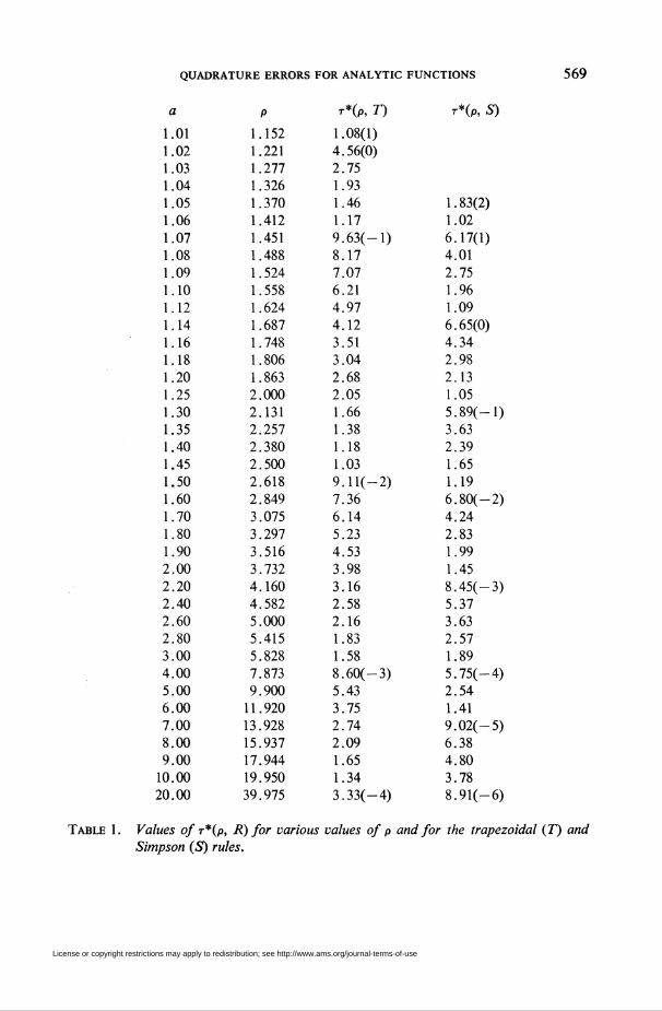
The values r*(7', p) and r*iS, p) are given in Table 1 for various values of p.

4. For each integration rule R and each value of p, (15) defines the value of the

norm of the error functional £(/). The question then arises to find particular rules

which minimize the value of r. This has been done by Barnhill and Wixom [1] with

respect to the norm a for two different cases, and we do the same for r. In the first

case, the abscissas are held fixed and the weights are chosen which minimize r. In

the second case, both the abscissae and the weights of an «-point rule are allowed to

vary so as to minimize t. In both cases, it is possible to impose constraints on the

rules such as the constraint that the rules integrate constants exactly, i.e., $Z*_, w\ = 2.



We computed unconstrained minimum norm rules for n = 2, 3, 4 and various

values of p and similar rules for fixed abscissae. We also computed corresponding

rules subject to the constraint that J^w,- = 2. These rules are essentially of no prac-

tical interest so that we shall not list them here. From the theoretical point of view,

their asymptotic properties are of interest and these are discussed in [10]. For the

present, we remark that the values of the minimum norm | |jR„| | are about half those

of riGn, p) for small values of p while, for large values of p, they are almost equal, and

the abscissae and weights of the minimum norm rules approach those of the corre-

sponding Gaussian rule. It is an easy matter to prove that, for any n, the limit as p

tends to infinity of any minimum norm rule is the n-point Gaussian rule. The proof

is based on the fact that for large p,

2 2 \EiTk)\2r iR, p) ~-~Tk— ,

IT p

where k is the first integer such that EÇTn) ̂ 0. For the 7i-point Gaussian rule, k = 2n

while for any other rule, k < 2n. Hence, any rule which minimizes t must tend to G„.

5. In this section we shall extend some results of Davis [4] on interpolatory

quadrature to the space L2(«p). Consider a scheme of quadratures of the form

(32; / fix) dx~Yl H-„t/(xnt) = /„(/), n = 1, 2, •• • .J\ k-0

It is said to converge uniformly in L'\B) if, given « > 0, there exists 7i0 = 7i0(e)

such that for all / G L'\B) and tj ^ 770, \EJJ)\ = l/i, fix) dx - /„(f)| á e||/||.Here L'2(5) is the set of functions analytic within the region B containing [—1, 1]

such that ÍÍb \f\2 dx dy is finite, in which case the integral equals 11/| |'2. Davis proved

that a necessary and sufficient condition that (32) converged uniformly in L'\B) is

that lim„_co ||£n||'2 = 0. A similar result can be shown to hold for L2(5), the set of

functions analytic within B such that fB |/(z)|2|l — z2\'1/2\dz\ is finite, where ||/||2 is

defined accordingly.

Davis then showed that a necessary and sufficient condition that (32) converge

uniformly in L'\ep) is that

(33) lim - ¿ (* + 1) M[fniUt)L=s = 0.n-.oo IT i_o P — P

A similar result holds for L2(ep), with (33) replaced by

tw lim 2 V l£"(r*>l2 - n(34) lim - ¿_, 2* , =2* — 0.»-.» 7T t_o P -+• P

Let us now define an interpolatory quadrature scheme as one for which E„if) = 0

if / is a polynomial of degree ^ n, and let us set M„ = 2Zï_0 \wkn\ è 2. Then Davis

showed that a sufficient condition that an interpolatory quadrature scheme converge

uniformly in L'2(ep) is that limn^„ M„n3/2P'n = 0. For L2(Ép), the condition is slightly

weaker, as given in the following theorem.

Theorem. Let limn_„ Mnp~n = 0. Then the interpolatory quadrature scheme

converges uniformly in L2(ep).



1.011.021.031.041.051.06

1.071.081.091.101.121.141.161.181.201.251.301.351.401.451.501.601.701.801.902.002.202.402.602.803.004.00

5.006.00

7.008.009.00

10.0020.00

P

1.1521.2211.277

1.3261.3701.4121.4511.4881.5241.5581.6241.6871.7481.8061.8632.0002.131

2.2572.3802.5002.6182.8493.0753.2973.5163.7324.1604.5825.0005.4155.8287.8739.900

11.92013.92815.93717.94419.95039.975

r*iP, T)

1.08(1)4.56(0)2.751.931.461.179.63(-l)8.177.076.214.974.12

3.513.042.682.051.661.381.181.039.11(-2)7.366.145.234.533.983.162.582.161.831.588.60(-3)5.433.752.742.091.651.343.33(-4)

r*(p, S)

1.83(2)1.026.17(1)4.012.751.961.09

6.65(0)4.342.982.131.055.89(-l)3.632.391.651.196.80(-2)4.242.831.991.458.45(-3)5.373.632.571.895.75(-4)2.541.419.02(-5)6.384.803.788.91(-6)

Table 1. Values of r*ip, R) for various values of p and for the trapezoidal (7) and

Simpson iS) rules.



Proof. We have

\rréïf - S W«™1tíríi p + p

Since p2* g p" + p"2t g 2p2\ we have

» ,2 I , + Ê k„,| |rt(xni)|Ca ||£,||2 ú £ -—!—^-

¡fc-m-1 P

á ¿ (t^-T + Mn)\-2k g [4 + ^ + M2] ± p"»r^íi \k — 1 / L« tí J tirÍ!

= |"4 + ^ + Ml\ -f^- = Csp-2n + CtM^p-2" + C.Mlp\_n n J p — 1

2 -Ib

Therefore, lim„_„, Mnp " = 0 implies lim„_„, ||£„||2 = 0. For Newton-Cotes integra-

tion rules,

^ < 4(1 + gn)2n 4(1 + 6Q

n(Iog n) n log n

where ô„, en —> 0 as tí —» ». The condition of the above theorem then holds for

p ^ 2. Therefore, the Newton-Cotes quadrature scheme converges uniformly in

.L2(ep) whenever p^2, Davis' analogous result for Z/2(ip) holds with p > 2.

Department of Applied Mathematics

Weizmann Institute of Science

Rebovot, Israel

1. R. E. Barnhill & J. A. Wixom, "Quadratures with remainders of minimum norm. I,H," Math. Comp., v. 21, 1967, pp. 66-75, 382-387. MR 36 #6138; MR 36 #6139.

2. M. M. Chawla, "Asymptotic estimates for the error of the Gauss-Legendre quadratureformula," Comput. I., v. 11, 1968/69, pp. 339-340. MR 38 #5389.

3. P. J. Davis, "Errors of numerical approximation for analytic functions," /. RationalMech. Anal., v. 2, 1953, pp. 303-313. MR 14, 907.

4. P. J. Davis, Errors of Numerical Approximation for Analytic Functions, Survey of Nu-merical Analysis, McGraw-Hill, New York, 1962, pp. 468-484. MR 24 #B1766.

5. P. J. Davis, Interpolation and Approximation, Blaisdell, Waltham, Mass., 1963. MR28 #393.

6. P. J. Davis & P. Rabinowitz, "On the estimation of quadrature errors for analyticfunctions," MTAC, v. 8, 1954, pp. 193-203. MR 16, 404.

7. G. HXmmerlin, "Zur Abschätzung von Quadraturfehlern für analytische Funktionen,"Numer. Math., v. 8, 1966, pp. 334-344. MR 34 #2179.

8. D. Nicholson, P. Rabinowitz, N. Richter & D. Zeilberger, "On the Error in theNumerical Integration of Chebyshev Polynomials," Math. Comp., v. 25, 1971.

9. P. Rabinowitz, "Practical error coefficients for estimating quadrature errors for ana-lytic functions," Comm. ACM, v. 11, 1968, pp. 45-46, MR 39 #2324.

10. P. Rabinowitz & N. Richter, "Asymptotic properties of minimal integration rules,"Math. Comp., v. 24, 1970, pp. 593-609.

11. A. H. Stroud & Û. Secrest, Gaussian Quadrature Formulas, Prentice-Hall, Engle-wood Cliffs, N. J., 1966. MR 34 #2185.


Date post:	01-Feb-2017
Category:	Documents
Upload:	nira
View:	212 times
Download:	0 times

New error coefficients for estimating quadrature errors for analytic functions

Documents