ORIGINAL PAPER - PRODUCTION ENGINEERING

New explicit correlation for the compressibility factor of naturalgas: linearized z-factor isotherms

Lateef A. Kareem1• Tajudeen M. Iwalewa2 • Muhammad Al-Marhoun3

Received: 14 October 2014 /Accepted: 17 October 2015 / Published online: 18 December 2015

� The Author(s) 2015. This article is published with open access at Springerlink.com

Abstract The compressibility factor (z-factor) of gases is

a thermodynamic property used to account for the devia-

tion of real gas behavior from that of an ideal gas. Corre-

lations based on the equation of state are often implicit,

because they require iteration and are computationally

expensive. A number of explicit correlations have been

derived to enhance simplicity; however, no single explicit

correlation has been developed for the full range of pseudo-

reduced temperatures 1:05� Tpr � 3� �

and pseudo-reduced

pressures 0:2�Ppr � 15� �

, which represents a significant

research gap. This work presents a new z-factor correlation

that can be expressed in linear form. On the basis of Hall

and Yarborough’s implicit correlation, we developed the

new correlation from 5346 experimental data points

extracted from 5940 data points published in the SPE

natural gas reservoir engineering textbook and created a

linear z-factor chart for a full range of pseudo-reduced

temperatures ð1:15� Tpr � 3Þ and pseudo-reduced pres-

sures ð0:2�Ppr � 15Þ.

Keywords Z-factor � Explicit correlation � Reducedtemperature � Reduced pressure � Natural gas

List of symbols

P Pressure (psi)

Ppc Pseudo-critical pressure

Ppr Pseudo-reduced pressure

T Temperature (R)

Tpc Pseudo-critical temperature (R)

Tpr Pseudo-reduced temperature

Ppc Pseudo-critical pressure (psi)

Ppr Pseudo-reduced pressure

v Initial guess for iteration process

Y Pseudo-reduced density

z-factor Compressibility factor

Introduction

The compressibility factor (z-factor) of gases is used to

correct the volume of gas estimated from the ideal gas

equation to the actual value. It is required in all calculations

involving natural gases.

The z-factor is the ratio of the volume occupied by a

given amount of a gas to the volume occupied by the same

amount of an ideal gas:

z ¼ Vactual

Videal

ð1Þ

Substituting for Videal in the ideal gas equation

PVactual ¼ znRT ð2Þ

For generalization, the z-factor is expressed as a

function of pseudo-reduced temperature and pressure

& Lateef A. Kareem

talk2laton@gmail.com

Tajudeen M. Iwalewa

tmi21@cam.ac.uk

Muhammad Al-Marhoun

marhoun@restec.com

1 Center for Petroleum and Minerals, King Fahd University of

Petroleum and Minerals, Dhahran, Saudi Arabia

2 Department of Earth Sciences, University of Cambridge,

Cambridge CB2 3EQ, UK

3 Reservoir Technologies (ResTec), Dammam, Saudi Arabia

123

J Petrol Explor Prod Technol (2016) 6:481–492

DOI 10.1007/s13202-015-0209-3

(Trube 1957; Dranchuk et al. 1971; Abou-kassem and

Dranchuk 1975; Sutton 1985; Heidaryan et al. 2010).

Dranchuk et al. (1971) defined pseudo-reduced tem-

perature and pressure as the ratio of temperature and

pressure to the pseudo-critical temperature and pressure of

natural gas, respectively:

Tpr ¼T

Tpc; Ppr ¼

P

Ppc

ð3Þ

The pseudo-critical properties of gas are the molar

abundance (mole fraction weighted) mean of the critical

properties of the constituents of the natural gas:

Tpc ¼Xn

i¼1

yiTci; Ppc ¼Xn

i¼1

yiPci ð4Þ

As a function of specific gravity (air = 1.0), Sutton

(1985) provides

Tpc ¼ 169:2þ 349:5cg � 74:0c2g ð5Þ

Ppc ¼ 756:8� 131:07cg � 3:6c2g ð6Þ

A plot of 5346 data points covering a full range of

pseudo-reduced temperatures ð1:15� Tpr � 3Þ and pseudo-

reduced pressures ð0:2�Ppr � 15Þ is shown in Fig. 1

Implicit z-factor correlations

The three most popular correlations for calculating the

z-factor are implicit. The three correlations, described in

the following subsections, are well known for their accu-

racies, almost unit correlation of regression coefficients and

low maximum errors.

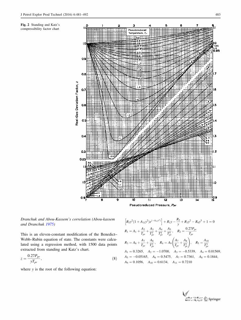
Hall and Yarborough’s correlation (Trube 1957)

Hall and Yarborough’s correlation is a modification of the

hard sphere Carnahan–Starling equation of state, with

constants developed through regression, and 1500 data

points extracted from Standing and Katz’s original z-factor

chart, as shown in Fig. 2.

z ¼ A1Ppr

y; ð7Þ

where y is the root of the following equation:

� A1Ppr þyþ y2 þ y3 � y4

ð1� yÞ3� A2y

2 þ A3yA4 ¼ 0

A1 ¼ 0:06125te�1:2ð1�tÞ2 ; A2 ¼ 14:76t � 9:76t2 þ 4:58t3;

A3 ¼ 90:7t � 242:2t2 þ 42:4t3; A4 ¼ 2:18þ 2:82t; t ¼ 1

Tpr

Fig. 1 Plot of experimental

measurements of the z-factor

482 J Petrol Explor Prod Technol (2016) 6:481–492

123

Dranchuk and Abou-Kassem’s correlation (Abou-kassem

and Dranchuk 1975)

This is an eleven-constant modification of the Benedict–

Webb–Rubin equation of state. The constants were calcu-

lated using a regression method, with 1500 data points

extracted from standing and Katz’s chart.

z ¼ 0:27Ppr

yTpr; ð8Þ

where y is the root of the following equation:

R5y2ð1þ A11y

2Þeð�A11y2Þ

h iþ R1y�

R2

yþ R3y

2 � R4y5 þ 1 ¼ 0

R1 ¼ A1 þA2

Tprþ A3

T3pr

þ A4

T4pr

þ A5

T5pr

; R2 ¼0:27Ppr

Tpr

R3 ¼ A6 þA7

Tprþ A8

T2pr

; R4 ¼ A9

A7

Tprþ A8

T2pr

!

; R5 ¼A10

T3pr

A1 ¼ 0:3265; A2 ¼ �1:0700; A3 ¼ �0:5339; A4 ¼ 0:01569;

A5 ¼ �0:05165; A6 ¼ 0:5475; A7 ¼ 0:7361; A8 ¼ 0:1844;

A9 ¼ 0:1056; A10 ¼ 0:6134; A11 ¼ 0:7210

Fig. 2 Standing and Katz’s

compressibility factor chart

J Petrol Explor Prod Technol (2016) 6:481–492 483

123

Dranchuk, Purvis and Robinson’s Correlation (Dranchuk

et al. 1971)

This is a further modification of the earlier obtained DAK

correlation. The DPR has eight constants and requires less

computational workload to obtain the z-factor.

z ¼ 0:27Ppr

yTpr; ð9Þ

where y is the root of the following equation:

T4y2ð1þ A8y

2Þeð�A8y2Þ

h iþ 1þ T1yþ T2y

2 þ T3y5 þ T5

y¼ 0

T1 ¼ A1 þA2

Tprþ A3

T3pr

; T2 ¼ A4 þA5

Tpr; T3 ¼

A5A6

Tpr;

T4 ¼A7

T3pr

; T5 ¼0:27Ppr

Tpr

A1 ¼ 0:31506237; A2 ¼ �1:04670990;

A3 ¼ �0:57832720; A4 ¼ 0:53530771;

A5 ¼ �0:61232032; A6 ¼ �0:10488813;

A7 ¼ 0:68157001; A8 ¼ 0:68446549

These correlations are effective; however, they do not

converge (or converge on wrong pseudo-reduced density

values) when the temperature of the systems is close to the

critical temperature. In addition, they are computationally

expensive. It is these limitations that necessitated the

development of the current explicit correlations.

Explicit correlations

Explicit correlations do not require an iterative procedure.

Therefore, they do not have the problem of convergence as

opposed to implicit correlations. One of the best explicit

correlations for evaluation of the z-factor was given by

Beggs and Brills (1973). More recent ones are Heidaryan

et al. (2010), Azizi et al. (2010) and Sanjari and Lay (2012)

correlations. A short description of some of the explicit

correlations is presented in the following subsections.

Brill and Beggs’ compressibility factor (1973)

z ¼ Aþ 1� A

eBþ CpDpr;

where

A ¼ 1:39ðTpr � 0:92Þ0:5 � 0:36Tpr � 0:10;

B ¼ ð0:62� 0:23TprÞppr þ0:066

Tpr � 0:86� 0:037

� �p2pr þ

0:32p2pr10E

C ¼ 0:132� 0:32 logðTprÞ; D ¼ 10F ;

E ¼ 9ðTpr � 1Þ and F ¼ 0:3106� 0:49Tpr þ 0:1824T2pr

Heidaryan, Moghdasi and Rahimi’s Correlation

Heidaryan et al. (2010) developed a new explicit

piecewise correlation using regression analysis of the

z-factor experimental value for reduced pseudo-pres-

sure of fewer and [3 (Table 1). The correlation has a

total of 22 constants, with a discontinuity at Ppr ¼ 3

(Fig. 2) and correlation regression coefficient of

0.99,963.

z ¼ lnA1 þ A3 lnðPprÞ þ A5

Tprþ A7 lnðPprÞ

� �2þ A9

T2prþ A11

TprlnðPprÞ

1þ A2 lnðPprÞ þ A4

Tprþ A6 lnðPprÞ

� �2þ A8

T2prþ A10

TprlnðPprÞ

0

@

1

A

ð11Þ

For some petroleum engineering applications, it is

often necessary to compute the derivative of z-factor

with respect to pressure or temperature. A function that

is discontinuous at a certain point is not differentiable at

that point (O’Neil 2012). Therefore, the explicit

correlation developed by Heidaryan et al. (2010)

cannot be used to evaluate the derivative of the z-

factor with respect to the pseudo-reduced pressure at

Ppr ¼ 3 (Fig. 3).

Azizi, Behbahani and Isazadeh’s Correlation

Azizi et al. (2010) presented an explicit correlation with 20

constants for a reduced temperature range of 1:1� Tpr � 2

and reduced pressure range of 0:2�Ppr � 11. The corre-

lation used 3038 data points within the given ranges.

z ¼ Aþ Bþ C

Dþ E; ð12Þ

where

Table 1 Constants of Heidaryan et al.’s correlation

Constants for Ppr � 3 Constants for Ppr [ 3

A1 2.827793 3.252838

A2 -4.688191 9 10-1 -1.306424 9 10-1

A3 -1.262288 6.449194 9 10-1

A4 -1.536524 -1.518028

A5 -4.535045 -5.391019

A6 6.895104 9 10-2 -1.379588 9 10-2

A7 1.903869 9 10-1 6.600633 9 10-2

A8 6.200089 9 10-1 6.120783 9 10-1

A9 1.838479 2.317431

A10 4.052367 9 10-1 1.632223 9 10-1

A11 1.073574 5.660595 9 10-1

484 J Petrol Explor Prod Technol (2016) 6:481–492

123

A ¼ aT2:16pr þ bP1:028

pr þ cP1:58pr T�2:1

pr þ d ln T�0:5pr

� �

B ¼ eþ fT2:4pr þ gP1:56

pr þ hP0:124pr T3:033

pr

C ¼ i ln T�1:28pr

� �þ j ln T1:37

pr

� �þ k ln Ppr

� �þ l ln P2

pr

� �

þ m lnðPprÞ lnðTprÞD ¼ 1þ nT5:55

pr þ oP0:68pr T0:33

pr

E ¼ p ln T1:18pr

� �þ q ln T2:1

pr

� �þ r lnðPprÞ þ s ln P2

pr

� �

þ t lnðPprÞ lnðTprÞ

a ¼ 0:0373142485385592; b ¼ �0:0140807151485369;

c ¼ 0:0163263245387186; d ¼ �0:0307776478819813;

e ¼ 13843575480:943800; f ¼ �16799138540:763700;

g ¼ 1624178942:6497600; h ¼ 13702270281:086900;

i ¼ �41645509:896474600; j ¼ 237249967625:01300;

k ¼ �24449114791:1531; l ¼ 19357955749:3274;

m ¼ �126354717916:607; n ¼ 623705678:385784;

o ¼ 17997651104:3330; p ¼ 151211393445:064;

q ¼ 139474437997:172; r ¼ �24233012984:0950;

s ¼ 18938047327:5205; t ¼ �141401620722:689;

Sanjari and Nemati’s Correlation

Using 5844 data points, Sanjari and Lay (2012) developed

an explicit correlation for the z-factor. This correlation, as

with Heidaryan et al. (2010) correlation, has different

constants for the values of Ppr below and above 3, but a

total of 16 constants (Table 2). The procedure for calcu-

lating the z-factor is as follows:

Fig. 3 Heidaryan et al.’s (2010)

correlation showing

discontinuity at Ppr � 3

Table 2 Constants of Sanjari and Lay’s correlation

Constants for Ppr � 3 Constants for Ppr [ 3

A1 0.007698 0.015642

A2 0.003839 0.000701

A3 -0.467212 2.341511

A4 1.018801 -0.657903

A5 3.805723 8.902112

A6 -0.087361 -1.136000

A7 7.138305 3.543614

A8 0.083440 0.134041

J Petrol Explor Prod Technol (2016) 6:481–492 485

123

z ¼ 1þ A1Ppr þ A2P2pr þ

A3PA4pr

TA5pr

þ A6PðA4þ1Þpr

TA7pr

þ A8PðA4þ2Þpr

TðA7þ1Þpr

ð13Þ

This correlation, however, is less efficient when

compared with that of Heidaryan et al. (2010). Its

regression correlation coefficient is 0.8757 and its error

rate at a certain point can be as high as 90 per cent. For

instance, the actual value of z from the experiment for a Ppr

of 15 and a Tpr of 1.05 is 1.753, but this correlation gives a

value of 3.3024. Therefore, the actual maximum error for

this correlation is 104.3206 %.

To resolve the limitations in the application of the

existing explicit correlations, a single correlation that is

continuous over the entire range of pseudo-reduced pres-

sure is required.

New explicit z-factor correlation

A new explicit z-factor is developed as a multi-stage cor-

relation based on Hall and Yarborough’s implicit correla-

tion. The implicit correlation was rearranged to return a

value of y using an approximate value of z. The y-values on

the right side of the expression were replaced by

A1Ppr=z� �

. Non-linear regression was performed using the

derived model. The resulting correlation for reduced den-

sity is given in Eq. 15, while Eq. 14 provides an extra

iteration to bring the results closer to those obtained by

Hall and Yarborough. The constants for these two equa-

tions are shown in

Table 3. The z-factor chart shown in Fig. 4 was gener-

ated from this new correlation:

Table 3 Constants of the new correlation

Constants

a1 0.317842 a11 -1.966847

a2 0.382216 a12 21.0581

a3 -7.768354 a13 -27.0246

a4 14.290531 a14 16.23

a5 0.000002 a15 207.783

a6 -0.004693 a16 -488.161

a7 0.096254 a17 176.29

a8 0.166720 a18 1.88453

a9 0.966910 a19 3.05921

a10 0.063069

Fig. 4 Plot of z-factor

generated using Eq. 14

486 J Petrol Explor Prod Technol (2016) 6:481–492

123

z ¼ DPprð1þ yþ y2 � y3ÞðDPpr þ Ey2 � FyGÞð1� yÞ3

ð14Þ

y ¼ DPpr

1þA2

C� A2B

C3

� � ; ð15Þ

where

t ¼ 1

Tpr;

A ¼ a1tea2ð1�tÞ2Ppr; B ¼ a3t þ a4t

2 þ a5t6P6

pr;

C ¼ a9 þ a8tPpr þ a7t2P2

pr þ a6t3P3

pr

D ¼ a10tea11ð1�tÞ2 ; E ¼ a12t þ a13t

2 þ a14t3;

F ¼ a15t þ a16t2 þ a17t

3; G ¼ a18 þ a19t

Linearized z-factor isotherms

Given that the reduced temperature and pressure fall within

1:15� Tpr � 3 and 6�Ppr � 15, the first nine constants can

be used to predict z with a correlation regression coefficient

of 0.99899. For this range of pseudo-reduced properties,

the simplified single-stage correlation of the z-factor is

given by

z ¼ 1þ A2

C� A2B

C3ð16Þ

A plot of Eq. 16 is shown in Fig. 5.

A careful analysis of Eq. 16 shows that it can be

rewritten in the following form:

zC ¼ 1þMP2pr 1� B

C2

� �ð17Þ

The values of M are chosen to be a function of reduced

temperature and a regression analysis performed to extend

the applicability of Eq. 17 to cover the ranges

1:15� Tpr � 3 and 0:2�Ppr � 15. For this range of

values of reduced temperature and pressure, M is given by

M ¼ m1t2em2ð1�tÞ2 ;

m1 ¼ 0:1009332; m2 ¼ 0:7773702

It should be noted that B and C maintain the same

definition as in Eq. 16. Hence, a graph of zC against

P2pr 1� B

C2

� �gives straight lines passing through the point

P2pr 1� B

C2

� �¼ 0; zC ¼ 1

� �with slopes M. A plot of the

straight line form of the z-factor is shown in Fig. 6.

Fig. 5 Plot of z-factor

generated using Eq. 16

J Petrol Explor Prod Technol (2016) 6:481–492 487

123

Results and discussion

Figure 7 shows the cross plot of the z-factor from the new

correlation against the measured values. The cross plots

show that the plotted points fall on the unit slope line

through the origin, which implies that the new correlation

reproduces the measured values to a considerable degree of

accuracy.

Table 4 shows the statistical detail of the constants of

the new correlation. The narrowness of the 95 per cent

confidence interval is in agreement with the near-zero

P-values. This implies that the probability that these values

could have been developed by chance is negligible, which

signifies that the new correlation is reliable (Wolberg

2006).

As shown in Table 5, within the range of pseudo-re-

duced temperatures ð1:15� Tpr � 3Þ and pseudo-reduced

pressures ð0:2�Ppr � 15Þ, Eq. 14 outperforms Heidaryan

et al.’s (2010) correlation in terms of correlation regression

coefficient, average percentage error and root mean square

of error, with the exception of maximum percentage error.

Most importantly, the new correlation is continuous over

the entire pseudo-pressure range. Therefore, it would allow

for computation of the derivatives of the z-factor over the

whole range ð0:2�Ppr � 15Þ, which is not possible with

other explicit correlations.

An application of the new correlation shown in Eq. 17

produces a good correlation of regression of 0.9999

between zexpC and 1þMP2pr 1� B

C2

� �. The maximum

relative error is the same as that in Eq. 14. This maximum

error is shown in Fig. 8 to occur at Ppr ¼ 2 and

Tpr ¼ 1:15.

Plots of the z-factors generated using the three most

recent explicit correlations (Sanjari and Lay 2012; Hei-

daryan et al. 2010; Azizi et al. 2010) were compared with

those generated using Eqs. 14 and 16 (Fig. 9). While

Sanjari and Lay (2012) and Azizi et al. (2010) show

marked deviations from the unit line, Heidaryan et al.

(2010) and Eqs. 14 and 16 fall on the unit line. This shows

that the correlations of Heidaryan et al. (2010) and Eqs. 14

and 16 (and by extension Eq. 17) are better at predicting

the values of the z-factor than those of Sanjari and Lay

(2012) and Azizi et al. (2010). Since these functions have

no point of discontinuity, they can be used in applications

where the derivative of the z-factor with respect to its

independent variables is required.

Fig. 6 Linear form z-factor

chart using Eq. 17

488 J Petrol Explor Prod Technol (2016) 6:481–492

123

Fig. 7 Cross plot of correlation

estimate against measured

z-factor

Table 4 Statistical detail of the constants of the new correlation

Constants Estimated values 95 % confidence interval P values Correlation regression coefficient

a1 0.317842 {0.316999, 0.318686} 5.9718379920 9 10-5841 0.999864

a2 0.382216 {0.379011, 0.385422} 2.53091273354 9 10-2995

a3 -7.76835 {-7.95029, -7.58642} 4.4950402736 9 10-1007

a4 14.2905 {14.071, 814.5093} 5.1169104227 9 10-1710

a5 2.18363 9 10-6 {2.13411, 2.23314} 9 10-6 8.8734666722 9 10-1053

a6 -0.00469257 {-0.00476861, -0.00461652} 4.4906844765 9 10-1604

a7 0.0962541 {0.095078, 0.0974301} 2.43824633475 9 10-2160

a8 0.16672 {0.160731, 0.17271} 2.01035053289 9 10-526

a9 0.96691 {0.964676, 0.969145} 2.17145789885 9 10-6193

a10 0.063069 {0.0624199, 0.0637180} 2.4388910420 9 10-556 0.999945

a11 -1.966847 {-1.97194278, -1.96175122} 2.8734273447 9 10-292

a12 21.0581 {20.7208, 21.3954} 1.17296332188 9 10-1625

a13 -27.0246 {-28.0223, -26.0269} 2.14835618371 9 10-503

a14 16.23 {15.5168, 16.9432} 4.28626039700 9 10-375

a15 207.783 {203.66, 211.906} 9.1427403949 9 10-1256

a16 -488.161 {-499.149, -477.174} 1.48225067124 9 10-1063

a17 176.29 {169.521, 183.06} 1.40366406588 9 10-471

a18 1.88453 {1.87601, 1.89306} 4.6430138718 9 10-4494

a19 3.05921 {3.03467, 3.08375} 5.5399223318 9 10-3099

J Petrol Explor Prod Technol (2016) 6:481–492 489

123

Example calculations

With Figs. 1 and 5, evaluate and compare the compress-

ibility factor of a 0.7 gravity gas at 2000 psig and 150 �F.From Sutton’s (1985) correlation,

Tpc ¼ 169:2þ 349:5ð0:7Þ � 74:0ð0:7Þ2 ¼ 377:59R

Ppc ¼ 756:8� 131:07ð0:7Þ � 3:6ð0:7Þ2 ¼ 663:29psig

Solution 1

Tpr ¼150þ 460

377:59¼ 1:6155; Ppr ¼

2000

663:29¼ 3:0153

From Fig. 10, z ¼ 0:83

Solution 2

t ¼ 1

Tpr¼ 0:619; B ¼ a3t þ a4t

2 þ a5t6P6

pr ¼ 0:6670

C ¼ a9 þ a8tPpr þ a7t2P2

pr þ a6t3P3

pr ¼ 1:5829;

P2pr 1� B

C2

� �¼ 6:6713

From Fig. 11,

zC Tpr ¼ 1:6155;P2pr 1� B

C2

� �¼ 6:6713

� �¼ 1:32 ! z

¼ 1:32

1:5829¼ 0:8339

Fig. 8 Contour plot of relative

error

Table 5 Comparison of the explicit correlations with the experimental data

Models Maximum absolute

error

Coefficient of

regression

Maximum percentage

error

Average percentage

error

Root mean square of

percentage error

Sanjari and Lay (2012) 0.7664 0.94946 45.5651 3.7463 7.3258

Heidaryan et al. (2010) 0.0220 0.99963 3.71630 0.4876 0.7369

Azizi et al. (2010) 0.3543 0.87240 60.0251 13.5907 15.7493

Equation 14 0.0270 0.99972 5.9976 0.4379 0.6929

Equation 16 0.0396 0.99899 8.7970 0.8267 1.2430

490 J Petrol Explor Prod Technol (2016) 6:481–492

123

The problem can also be solved using Eq. 14 directly:

z ¼ DPprð1þ yþ y2 � y3ÞDPpr þ Ey2 � FyG� �

ð1� yÞ3ð18Þ

y ¼ DPpr

1þA2

C� A2B

C3

� � ; ð19Þ

where

A ¼ a1tea2ð1�tÞ2Ppr ¼ 0:62708; D ¼ a10te

a11ð1�tÞ2 ¼ 0:02934

E ¼ a12t þ a13t2 þ a14t

3 ¼ 6:56232; F ¼ a15t þ a16t2

þ a17t3 ¼ �17:08860

G ¼ a18 þ a19t ¼ 3:80547; y ¼ DPpr

1þA2

C� A2B

C3

� � ¼ 0:10869

Therefore,

z ¼ DPpr 1þ yþ y2 � y3ð ÞDPpr þ Ey2 � FyG� �

1� yð Þ3¼ 0:8242

Conclusions

A simple accurate correlation for evaluating the z-factor

that can be linearized has been developed. This corre-

lation performs excellently in the ranges 1:15� Tpr � 3

and 0:2�Ppr � 15. It is simple and single-valued. A

noteworthy advancement is that the new correlation is

continuous over the full range of pseudo-reduced

0.4 0.6 0.8 1 1.2 1.4 1.6 1.8

0.4

0.6

0.8

1

1.2

1.4

1.6

1.8

2

2.2

2.4

Experimentally determined z-factor

Z-f

acto

r ob

tain

ed f

rom

cor

rela

tions

Sanjari et alHeidaryan et alAzizi et alEquation 14Equation 16

Fig. 9 Cross plot comparing several explicit correlations

Fig. 10 Example illustration 1

J Petrol Explor Prod Technol (2016) 6:481–492 491

123

pressures ð0:2�Ppr � 15Þ. This will widen its applica-

bility to include cases such as the evaluation of natural

gas compressibility, in which the derivative of the

compressibility factor with respect to the pseudo-re-

duced pressure is required. For the range outside the

coverage of this correlation, implicit correlations can be

applied; however, this new explicit correlation can be

used to provide an initial guess to speed up the iteration

process.

Open Access This article is distributed under the terms of the

Creative Commons Attribution 4.0 International License (http://

creativecommons.org/licenses/by/4.0/), which permits unrestricted

use, distribution, and reproduction in any medium, provided you give

appropriate credit to the original author(s) and the source, provide a

link to the Creative Commons license, and indicate if changes were

made.

References

Azizi N, Behbahani R, Isazadeh MA(2010) An efficient correlation

for calculating compressibility factor of natural gases. J Nat Gas

Chem 19:642–645. doi:10.1016/S1003-9953(09)60081-5

Abou-kassem JH, Dranchuk PM (1975) Calculation of z factors for

natural gases using equations of state. J Can Pet Technol. doi:10.

2118/75-03-03

Beggs DHU, Brill JPU (1973) A study of two-phase flow in inclined

pipes. J Pet Technol 25:607–617

Dranchuk RA, Purvis DB, Robinson PM (1971) Generalized

compressibility factor tables. J Can Pet Technol 10:22–29

Heidaryan E, Salarabadi A, Moghadasi J (2010) A novel correlation

approach for prediction of natural gas compressibility factor.

J Nat Gas Chem 19:189–192. doi:10.1016/S1003-

9953(09)60050-5

O’Neil PV (2012) Advanced engineering mathematics, 7th edn.

Cengage Laerning, Stamford

Sanjari E, Lay EN (2012) An accurate empirical correlation for

predicting natural gas compressibility factors. J Nat Gas Chem

21:184–188. doi:10.1016/S1003-9953(11)60352-6

Sutton RP (1985) Compressibility factor for high-molecular-weight

reservoir gases. In: 60th annual technical conference and

exhibition of society of petroleum engineers

Trube A (1957) Compressibility of natural gases. J Pet Technol.

doi:10.2118/697-G

Wolberg J (2006) Data analysis using the method of least squares:

extracting the most information from experiments, 2nd edn.

Springer, Berlin

Fig. 11 Example illustration 2

492 J Petrol Explor Prod Technol (2016) 6:481–492

123