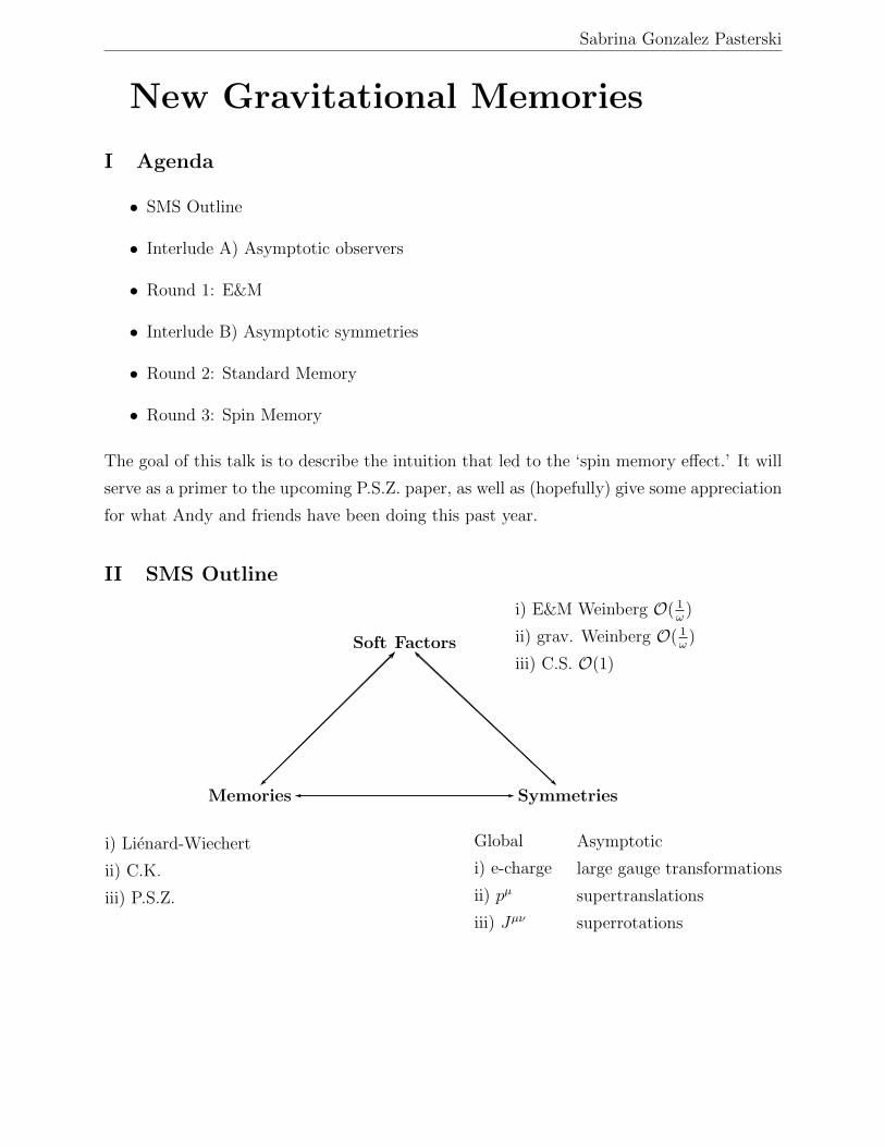
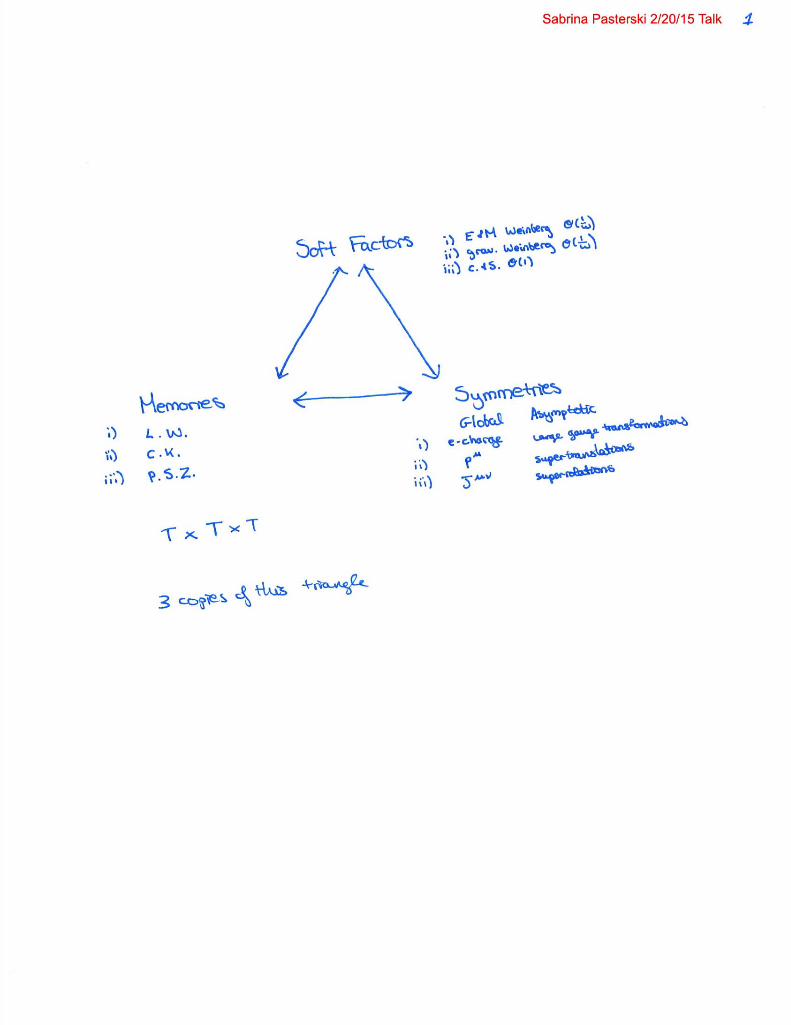
Sabrina Gonzalez Pasterski New Gravitational Memories I Agenda • SMS Outline • Interlude A) Asymptotic observers • Round 1: E&M • Interlude B) Asymptotic symmetries • Round 2: Standard Memory • Round 3: Spin Memory The goal of this talk is to describe the intuition that led to the ‘spin memory e↵ect.’ It will serve as a primer to the upcoming P.S.Z. paper, as well as (hopefully) give some appreciation for what Andy and friends have been doing this past year. II SMS Outline Soft Factors Memories Symmetries i) E&M Weinberg O( 1 ω ) ii) grav. Weinberg O( 1 ω ) iii) C.S. O(1) i) Li´ enard-Wiechert ii) C.K. iii) P.S.Z. Global i) e-charge ii) p μ iii) J μν Asymptotic large gauge transformations supertranslations superrotations
Transcript
Sabrina Gonzalez Pasterski
New Gravitational Memories
I Agenda
• SMS Outline
• Interlude A) Asymptotic observers
• Round 1: E&M
• Interlude B) Asymptotic symmetries
• Round 2: Standard Memory
• Round 3: Spin Memory
The goal of this talk is to describe the intuition that led to the ‘spin memory e↵ect.’ It will
serve as a primer to the upcoming P.S.Z. paper, as well as (hopefully) give some appreciation
for what Andy and friends have been doing this past year.
II SMS Outline
Soft Factors
Memories Symmetries
i) E&M Weinberg O( 1ω)
ii) grav. Weinberg O( 1ω)
iii) C.S. O(1)
i) Lienard-Wiechert
ii) C.K.
iii) P.S.Z.
Global
i) e-charge
ii) pµ
iii) Jµν
Asymptotic
large gauge transformations
supertranslations
superrotations
Sabrina Gonzalez Pasterski
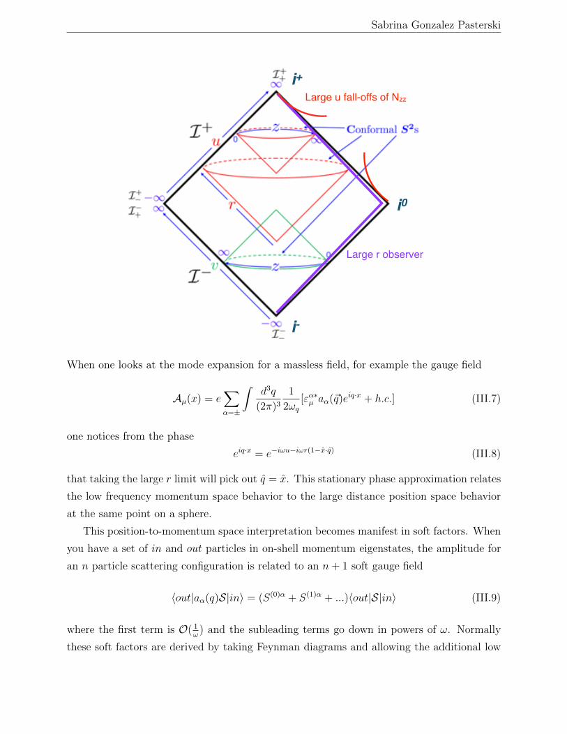
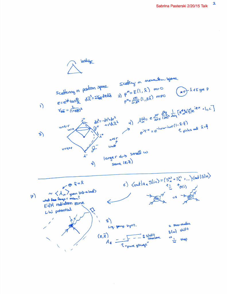
III Interlude A) Asymptotic observers
• conventions
• connection between position space (large r) and momentum space (small !)
The conformal compactification of Minkowski space gives a nice way to visualize the causal
structure. The diagram is drawn so that the left side vs. right side are the NP and SP of a
full S2. The retarded and advanced times
u = t� r, v = t+ r (III.1)
give the metric
ds
2 = �dt
2 + dr
2 + r
2d⌦2 = �dudv +
(v � u)2
4d⌦2
. (III.2)
Now letting
u = L tanU, v = L tanV (III.3)
gives
ds
2 =L
2
cos2 U cos2 V(�dUdV +
sin2(U � V )
4d⌦2) (III.4)
where U, V 2 {�⇡
2 ,⇡
2}.Massless particles come in along past null infinity I� and exit at future null infinity I+.
In this compactification, spatial infinity i
0 is a single point. This is one way of motivating
why
III.I Conventions
I will parameterize coordinates on the sphere with
z = e
i� tan✓
2, d⌦2 = 2�
zz
dzdz, �
zz
=2
(1 + zz)2(III.5)
I will be considering on-shell particles, whose momenta are described by their energy and a
point on the sphere
p
µ = E(1, x) massless
p
µ = m�(1, �x) massive(III.6)
Sabrina Gonzalez Pasterski
Large r observer
Large u fall-offs of Nzz
i-
i0
i+
When one looks at the mode expansion for a massless field, for example the gauge field
Aµ
(x) = e
X
↵=±
Zd
3q
(2⇡)31
2!q
["↵⇤µ
a
↵
(~q)eiq·x + h.c.] (III.7)
one notices from the phase
e
iq·x = e
�i!u�i!r(1�x·q) (III.8)
that taking the large r limit will pick out q = x. This stationary phase approximation relates
the low frequency momentum space behavior to the large distance position space behavior
at the same point on a sphere.
This position-to-momentum space interpretation becomes manifest in soft factors. When
you have a set of in and out particles in on-shell momentum eigenstates, the amplitude for
an n particle scattering configuration is related to an n+ 1 soft gauge field
hout|a↵
(q)S|ini = (S(0)↵ + S
(1)↵ + ...)hout|S|ini (III.9)
where the first term is O( 1!
) and the subleading terms go down in powers of !. Normally
these soft factors are derived by taking Feynman diagrams and allowing the additional low
Sabrina Gonzalez Pasterski
momentum photon to attach to all external legs. Vertex factors from the interactions deter-
mine the numerator, while the additional propagator gives the pole for the leading term.
These can equivalently be thought of as classical equations of motion, connecting soft
factors to memories.
IV Round 1: E&M
• radiation zone
• soft factor and expectation values
• intuition for boundary matching
A natural question to ask is how the I+ description carries over to large-but-finite r observers.
While on the Penrose diagram such an observer looks like it skirts I+, it is on a timelike,
rather than a null, trajectory. The answer is in the order of limits. By imposing fall o↵
conditions on the dynamical variables, one can focus on dynamics where u << r.
The simplest example is to consider the radiation sourced by an accelerated charge in
electromagnetism. The equation governing such radiation
@
u
A
u
= @
u
(Dz
A
z
+D
z
A
z
) + e
2j
u
(IV.1)
when integrated over time is a statement about the final versus initial charge-velocity dis-
tributions. With the identification
�A
z
= � 1
4⇡"
⇤+z
!S
(0)+ (IV.2)
coming from the mode expansion, saying that the soft factor gives the expectation value of
�A
z
means that the radial component of the electric field has the following contribution
from a single boosted charge:
lim!!0
![Dz
"
⇤+z
S
(0)+p
+D
z
"
⇤�z
S
(0)�p
] = Q
�
21
(1�~
�·n)2 (IV.3)
where
S
(0)±p
= Q
p · "±p · q (IV.4)
Note that simply plugging in the soft factor gives the electric field for a perpetually moving
particle. In terms of the position of the source at the retarded time, the Lienard-Weichert
Sabrina Gonzalez Pasterski
potential gives
E
r
=q
4⇡
1
�
2(1� ~
� · n)2|r � r
s
|2 (IV.5)
which is in exact agreement with plugging massive p
µ into the soft factor. This also yields
two important insights. 1. We can equivalently write an expression for the electric field of a
perpetually moving charge as a function of its current position. In this case
~
E =q
4⇡
1
�
2(1� �
2 sin2✓)
32
R
R
2(IV.6)
If the charge moves through the spacetime origin, towards the north pole for instance, then
a little bit after t = 0, it will be closer to the NP, whereas a little bit before, it will be closer
to the SP. The radial electric field thus obeys a natural “antipodal” matching of sorts. The
issue of matching across i0 is non-trivial, but one would hope that in the finite r limit, one
can still make sense of this type of matching, so an argument like this is helpful. 2. We can
think of these zero-mode position space measurements as telling us something about what
dynamics had to happen (i.e. radiation) given what came out versus what went in, when
considered as two separate static configurations.
Massless scattering a la LSET. Fields localized to shell emerging from spacetime origin
along u = 0. Start in vacuum, massless charges pass, vector potential changes as a result.
Between step functions, looks like “pure gauge” on the sphere. Large gauge transformations
e↵ectively allow you to “reset” your gauge field between any two wave fronts.
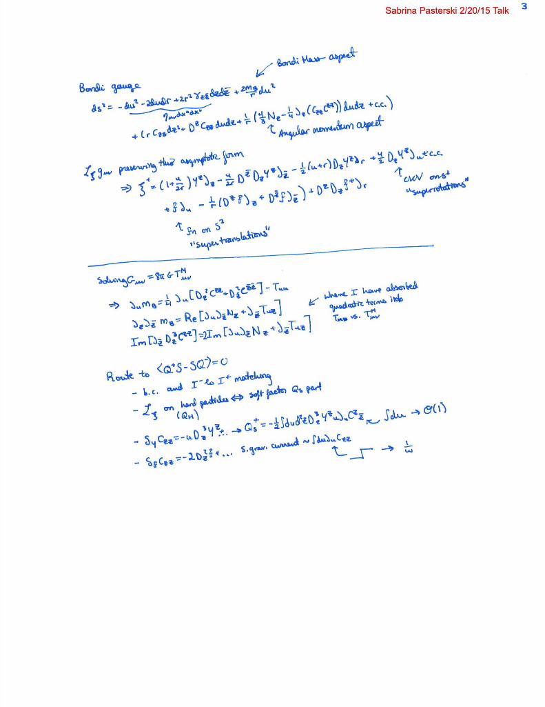
V Interlude B) Asymptotic symmetries
• Bondi Gauge
• supertranslation and superrotation vector fields
• G
uu
and G
uz
constraint equations
Asymptotically flat metrics in Bondi Gauge have the form
ds
2 = �du
2 � 2dudr + 2r2�zz
dzdz + 2mBr
du
2
+�rC
zz
dz
2 +D
z
C
zz
dudz + 1r
(43Nz
� 14@z(Czz
C
zz))dudz + c.c.
�+ ...
(V.1)
Key things to note about this gauge is that g
rr
= g
ra
= 0. C
zz
is a complex degree of
Sabrina Gonzalez Pasterski
freedom. The G
uu
and G
ua
O(r�2) constraint equations
G
µ⌫
= 8⇡GT
M
µ⌫
(V.2)
relate these to the Bondi mass and angular momentum aspect. From G
uu
@
u
m
B
= 14 [D
2z
N
zz +D
2z
N
zz]� T
uu
,
T
uu
⌘ 14Nzz
N
zz + 4⇡G limr!1
[r2TM
uu
],(V.3)
Taking @
z
of the G
uz
constraint and @
z
of the complex conjugate G
uz
constraint gives:
@
z
@
z
m
B
= Re[@u
@
z
N
z
+ @
z
T
uz
] (V.4)
Im[@z
D
3z
C
zz] = 2Im[@u
@
z
N
z
+ @
z
T
uz
]. (V.5)
There are two families of vector fields which preserve the asymptotic form of the metric:
supertranslations parameterized by an arbitrary scalar on the sphere and superrotations
corresponding to a Virasoro symmetry parametrized by a conformal killing vector.
⇠
+ =(1 +u
2r)Y +z
@
z
� u
2rD
z
D
z
Y
+z
@
z
� 1
2(u+ r)D
z
Y
+z
@
r
+u
2D
z
Y
+z
@
u
+ c.c. (V.6)
+ f
+@
u
� 1
r
(Dz
f
+@
z
+D
z
f
+@
z
) +D
z
D
z
f
+@
r
,
(Note that in the limit that one is near the u = 0 lightcone, the lorentz transformations look
like global conformal transformations of the sphere).
There are two limits in which solving the radiation constraint equations simplifies. 1)
Assume only outgoing radiation sourced by changes in the distribution of massive matter.
Then at linear order, the change on the left hand side gives the metric perturbations on the
right. 2) Assume only massless in and out states, then use boundary conditions to fix the
early and late time limits of the left hand side. This sets the stage for the scattering problem
and S-matrix connection.
These symmetries are turned into ward identities for massless scattering processes as
follows:
• set boundary conditions and matching between I� and I+.
• the Lie derivative gives the action of the symmetry on the hard particles
• limits to zero mode radiative brackets (special to d=4) motivate the conjugate zero-
Sabrina Gonzalez Pasterski
mode operator
• the lie derivative acting on the flat metric gives the inhomogeneous change generated
in the linear theory
– �
Y
C
zz
= �uD
3z
Y
z+...! Q
+S
= �12
Rdud
2zD
3z
Y
z
u@
u
C
z
z
– �
f
C
zz
= �2D2z
f+....! soft graviton current involvingRdu@
u
C
zz
verifying that the charges generated the symmetry via the soft factor amounted to showing
that the soft operator gave the appropriate Lie derivative acting on the hard states. (For
the super translation case, the charge reduced to an expression like the Bondi Mass aspect
in the first constraint equation.)
One important boundary condition worth mentioning here is that the curl of Czz
vanishes
at the limits of I+. This makes it possible for its integral to be finite, which we will see
relates to the spin memory e↵ect.
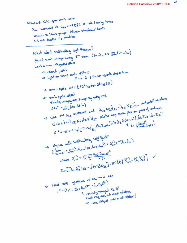
VI Round 2: Standard Memory
• soft factor and boosted mass
• Supertranslation charge �(!) and 1!
zero modes
• intepreting the metric
The boundary conditions on the metric imply that at early and late u
C
zz
= �2D2z
C (VI.1)
much like in the electromagnetic case, this looks like a pure supertranslation, though it really
indicates a transition between two di↵erent super translated vacuua.
Start in vacuum, shockwave passes, metric changes as a result but is still in an asymptoti-
cally flat form. Between wavefronts, looks like nothing is happening. BMS supertranslations
e↵ectively allow you to “reset” your metric between any two shock waves.
Here the conjugate zero modes are a shift and a step, with the step describing the
Weinberg pole and its conjugacy to the pure supertranslation shift defining the S matrix
ward identity. Comparing the metric at early and late times, one sees that a change in C
zz
amounts to a change in physical distances between objects at di↵erent points on a large r
sphere.
Sabrina Gonzalez Pasterski
S.Z. show that the leading soft factor amounts to the Braginsky Thorne result with the
expectation value position-to-momentum-space interpretation. Like the E&M case, on can
read o↵ from the constraint equation �m
B
cooresponding to a set of boosted masses, which
individually have the form
m
B
=m
�
3
1
(1� ~
� · n)3 (VI.2)
The massive soft factor contribution from a single particle
S
(0)±p
=(p · "±)2p · q (VI.3)
obeys
lim!!0
![Dz
D
z
"
⇤+zz
S
(0)+p
+D
z
D
z
"
⇤�zz
S
(0)�p
] = �m
�
31
(1�~
�·n)3 (VI.4)
where n is the unit vector pointing parallel to ~q and I have used
p
µ = m�(1, ~�). (VI.5)
The constraint equation gives:
@
u
m
B
=1
4D
2z
N
zz +1
4D
2z
N
zz � 1
2T
M
uu
� 1
4N
zz
N
zz
, (VI.6)
so that a linearized theory with no massless matter would have
�m
B
=1
4[D2
z
�C
zz +D
2z
�C
zz]. (VI.7)
From the stationary phase approximation, we identify �C
zz
as
�C
zz
= �
2
8⇡"
⇤+zz
!S
(0)+p
(VI.8)
reproducing the above.
VII Round 3: Spin Memory
• interpreting the metric
• thought experiment: the BMS ring
• rotation of inertial observers and D
A
C
AB
dx
B
Sabrina Gonzalez Pasterski
• Superrotation charge
K.L.P.S. showed that the superrotations corresponded to the subleading soft factor, which
essentially came from the soft charge Q
+S
= �12
Rdud
2zD
3z
Y
z
u@
u
C
z
z
picking out the order 1
soft factor due to the projection lim!!0
(1 + !@
!
) coming from the u integral.
This got me thinking about how to naturally construct a u integrated observable. The
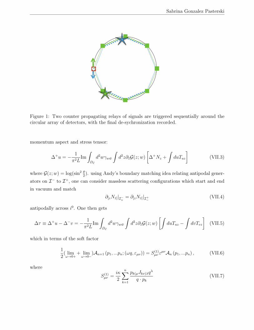
result was the following thought experiment. Imagine sending light rays around a ring
fixed to the BMS observer’s coordinates. The path that a beam will travel between two
nearby mirrors along this forced trajectory will be described by ds
2 = 0. If one looks at the
asymptotically flat metric in Bondi gauge, one will note that there are various places where
lengths will change, but there is one set of terms, namely the dudz and c.c. part that are
odd under �z ! ��z. If you have two beams going between the same mirrors in opposite
directions at the same time, then this would pick out that correction to the metric.
Now let us consider a small ring. If the metric does not change appreciably over the time
scale during which a beam circuits the ring, then over the course of one orbit, each segment
is e↵ectively transversed by two beams moving in opposite directions at e↵ectively “same
time” as regards the metric fluctuations. (Note that I can always scale the size of the ring
down so that this limit holds). Going in one direction is slightly faster than the other and
this curl part accumulates so that over the course of one orbit, I get a contour integral and
time delay
�P =
I
C(Dz
C
zz
dz +D
z
C
zz
dz) . (VII.1)
Now if I repeat the orbit again, the time delay accumulates. In the limit where the repetition
is much faster than the time delay, the net time accumulated delay is simply the time integral
of the curl of the metric divided by the period of the beam orbit:
�+u =
1
2⇡L
Zdu
I
C(Dz
C
zz
dz +D
z
C
zz
dz) . (VII.2)
This has multiple nice features, the most important of which is that it is insensitive to
supertranslations, or even superrotations for that matter. The final state of the metric will
be such that this curl is zero, and this the cumulative time delay will converge rather than
continue to build in a vacuum-equivalent configuration. It is analogous to a frame dragging
phenomenon, but is a zero-mode e↵ect and thus a new “gravitational memory.”
Using the constraint equations, one can rewrite this time delay in terms of the angular
Sabrina Gonzalez Pasterski
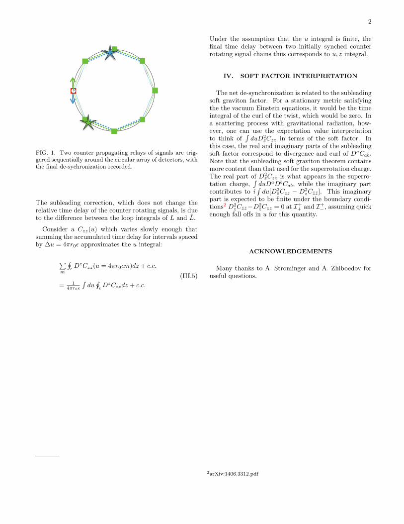
Figure 1: Two counter propagating relays of signals are triggered sequentially around thecircular array of detectors, with the final de-sychronization recorded.
momentum aspect and stress tensor:
�+u = � 1
⇡
2L
Im
Z
DC
d
2w�
ww
Zd
2z@
z
G(z;w)�+
N
z
+
ZduT
uz
�(VII.3)
where G(z;w) = log(sin2 ✓
2). using Andy’s boundary matching idea relating antipodal gener-
ators on I� to I+, one can consider massless scattering configurations which start and end
in vacuum and match
@[zNz]|I�+= @[zNz]|I+
�(VII.4)
antipodally across i0. One then gets
�⌧ ⌘ �+u���
v = � 1
⇡
2L
Im
Z
DC
d
2w�
ww
Zd
2z@
z
G(z;w)Z
duT
uz
�Z
dvT
vz
�(VII.5)
which in terms of the soft factor
1
2( lim!!0+
+ lim!!0�
)An+1 (p1, ...pn; (!q, "µ⌫)) = S
(1)µ⌫
"
µ⌫An
(p1, ...pn) , (VII.6)
where
S
(1)µ⌫
=i
2
nX
k=1
p
k(µJk⌫)�q�
q · pk
(VII.7)
Sabrina Gonzalez Pasterski
can be explicitly checked to match for a set of massless scatters. i.e.
Im⇥ Z
duD
2z
C
zz
�Z
dvD
2z
C
zz
⇤= 2iG[D2
z
S
(1)zz
�D
2z
S
(1)zz
]. (VII.8)
This boundary matching can be equivalently expressed as a new charge
Q(z, z) = i@[zNz](z, z)|I+�
(VII.9)
constraining angular momentum flux through antipodal contours in a scattering process.
As a final note, there is another way to interpret this spin memory in terms of inertial
observers. A massive geodesic at large r has a four velocity given by (suppressing the Bondi
mass term)
v
µ = (1, 0,� 1
2r2D
z
C
zz
,� 1
2r2D
z
C
zz) (VII.10)
The component of the velocity tangental to the two sphere is thus determined by the form
V ⌘ 14D
a
C
ab
dx
b. If one considers a rigid ring, it can resist deformations but will have no
means of resisting a net rotation. Thinking of the curl as the vorticity of a fluid, this time
integral is equivalent to a net rotation.
Depending on the relative scaling of the rotation with the size of the contour, it becomes
more appropriate or less to treat the ring as a BMS vs. geodesic observer. I.e. for spinning
particles passing through a ring the e↵ect scales down rapidly with distance, such that the
ring can be “held still,” whereas gravitational wave scaling is such that the local region
rotates together. While the first gyraton-like solution would expect a time delay, the second
would be better described by a net rotation relative to objects far away.
VIII Main Topics
• part that is measureable & part that is a symmetry
– � at boundaries $ supertranslations and an overall shift
– curl of vectorRdu of subleading behavior $ divergence of this vector field’s
subleading behavior and superrotations
• u << r conformal symmetry of the lightcone
– I+ vs stationary observer t ⇠ r + "
– order of limits and u fall-o↵ conditions
Sabrina Gonzalez Pasterski
• between shocks, looks like pure gauge
– massless scattering, LSET and the solution propagating out at u = 0
• match what happened on I� to beginning of what happens on I+.
– accelerations occurring at t = 0 don’t propagate until u = 0 to I+.
– look at boosted solutions on straight line trajectories through the spacetime origin.
– antipodal matching of electric charge radial field
• 2 zero modes, Weinberg pole conjugate to �(!) piece.
Speed Demon
Sabrina Gonzalez Pasterski(Dated: Dec 16, 2014)
This note proposes a detector arrangement/measurement corresponding to the subleading soft
Here, I will consider a particular scattering configurationwhere instead Czz = 0 both initially and finally. More-over, I will restrict myself to situations where the enve-lope of Czz(u) has a finite u integral at each point on thesphere. Under these conditions:R
duu@uCzz = uCzz|1�1 �RduCzz
= �RduCzz
(I.2)
where the boundary term can be dropped for quickenough Czz(u) fall-o↵s, which I will assume.
II. TWO DETECTOR PRIMER
Following S.&Z., I will consider detectors that are ata fixed r = r0, with �z = z
0 � z describing their angularseparation in complex coordinates. If we assume �z issmall, then:
L =2r0|�z|1 + zz
(II.1)
is their spatial separation using the standard flat metric:
ds
2F = �du
2 � 2dudr + 2r2�zzdzdz. (II.2)
When, in addition to the flat metric, there is a perturba-tion:
ds
2 = ds
2F + 2mB
r du
2
+rCzzdz2 +D
zCzzdudz + c.c.,
(II.3)
the trajectories of light rays traveling between detectorswill satisfy:
2r20�zz�z�z+r0Czz�z2+D
zCzz�zz0
u�z+c.c.�(�zz0u)2 = 0(II.4)
going from z ! z
0, whereas the reverse route will have:
2r20�zz�z�z+r0Czz�z2�D
zCzz�z0zu�z+c.c.�(�z0zu)
2 = 0(II.5)
a ISBN: 978-0-9863685-9-21arXiv:1411.5745v1.pdf
where the Bondi mass term is subleading in r0. Subtract-ing the two equations gives:
�zz0u� �z0zu = D
zCzz�z + c.c. (II.6)
While adding the two equations gives:
(�zz0u)2+(�z0zu)
2 = 4r20�zz�z�z+r0Czz�z2+c.c. (II.7)
Combing these yields:
�zz0u = L+
1
2[Dz
Czz�z + c.c.] (II.8)
�z0zu = L� 1
2[Dz
Czz�z + c.c.] (II.9)
where
L = L+r0
2L[Czz�z
2 + c.c.] (II.10)
III. SUBLEADING MEASUREMENT
Consider N detectors arranged in a regular polygonaround z=0.
zn = ✏e
i 2⇡nN
, n 2 {0, ..., N � 1} (III.1)
In the large N limit, one has:
z = ✏e
i�, �z = iz�� (III.2)
The di↵erence between a clockwise versus a counterclockwise circuit for a constant Czz is:
limN!1
N�1Pn=0
{�n,n+1u� �n+1,nu}
= limN!1
N�1Pn=0
D
zCzz(✏e
i 2⇡nN )i✏ei
2⇡nN
2⇡N + c.c.
=2⇡R0D
zCzz(z)iz��+ c.c.
=H✏ D
zCzzdz + c.c.
(III.3)
This is equivalent to sending the signal chains in oppositedirections around the array of detectors and looking atthe time di↵erence when the two pulses arrive at thestarting point after a single loop.Note that this is a cumulative e↵ect. The di↵erence in
timing is a correction to the net time for a single circuit,which is at leading order in r0 is:
L✏ = 4⇡r0✏. (III.4)
2
FIG. 1. Two counter propagating relays of signals are trig-
gered sequentially around the circular array of detectors, with
the final de-sychronization recorded.
The subleading correction, which does not change therelative time delay of the counter rotating signals, is dueto the di↵erence between the loop integrals of L and L.
Consider a Czz(u) which varies slowly enough thatsumming the accumulated time delay for intervals spacedby �u = 4⇡r0✏ approximates the u integral:
Pm
H✏ D
zCzz(u = 4⇡r0✏m)dz + c.c.
= 14⇡r0✏
Rdu
H✏ D
zCzzdz + c.c.
(III.5)
Under the assumption that the u integral is finite, thefinal time delay between two initially synched counterrotating signal chains thus corresponds to u, z integral.
IV. SOFT FACTOR INTERPRETATION
The net de-synchronization is related to the subleadingsoft graviton factor. For a stationary metric satisfyingthe the vacuum Einstein equations, it would be the timeintegral of the curl of the twist, which would be zero. Ina scattering process with gravitational radiation, how-ever, one can use the expectation value interpretationto think of
RduD
2zCzz in terms of the soft factor. In
this case, the real and imaginary parts of the subleadingsoft factor correspond to divergence and curl of Da
Cab.Note that the subleading soft graviton theorem containsmore content than that used for the superrotation charge.The real part of D2
zCzz is what appears in the superro-tation charge,
RduD
aD
bCab, while the imaginary part
contributes to i
Rdu[D2
zCzz � D
2zCzz]. This imaginary
part is expected to be finite under the boundary condi-tions2 D2
zCzz�D
2zCzz = 0 at I+
+ and I+� , assuming quick
enough fall o↵s in u for this quantity.
ACKNOWLEDGEMENTS
Many thanks to A. Strominger and A. Zhiboedov foruseful questions.