New Metamaterials (MMs) based on an Extended...

1

Microwave Electronics Lab

New Metamaterials (MMs) based on

an Extended Transmission Line (TL) Approach

for Novel Microwave

Components, Antennas and Reflectors

Applications


Outline

I. Anisotropic RH / LH 2D Structures

II. RH/LH Surface Plasmons

III. Novel Class of Leaky-Wave Reflectors______________________________________

IV. 2D Distributed Meta-StructuresExhibiting Focusing, Frequency-Scanning Radiation, SP next time

2


Anisotropic RH / LH Structures

Γ X

MY

xk

yk

0ω

1Rω 2Rω

1Lω2Lω

2 1 0 1 2L L R Rω ω ω ω ω< < < <

(b)

RH

Rβ

LH Lβ

−2

0

2

−3−2

−10

12

3

−8

−6

−4

−2

0

2

4

6

8

xkyk

( ),x yk kω

Brillouinzone

Γ

YX

M

(a)

0 0k cω =

radiation(leakage)

cone

0ω


2D Transmission Line Unit-Cell ModelsIsotropic RH

yz

x

RC

2RL

2RL2RL

2RL

2RL2 LC

RC

LL

Anisotropicx-RH & y-LH

sZ

2RL2 LC

yz

x x-RH

y-LH

LL

Isotropic LH2 LC

2 LC

2 LC2 LC

yz

x

( )

( )

( )

( )

( )

2

2

2

2

2

2

1SHUNT IMPEDANCE: , with 1

1 1 low-freq:

(capacitive)1

1 high-freq:

1 (ind

os

os

oss os L R

R

osos s

R eq

Req R

os

osos s eq

R

oseq L

R

Z j L CC

Z j jC C

CC C

Z j j LC

L LC

ω ω

ω ω

ω ωω

ω

ω ωω ω

ω ω

ω ω

ω ωω ω ω

ω

ω ωω

−= =

−< ⇒ = − = −

= =−

−> ⇒ = =

−= = uctive)

2RL

eqC

2RL

x-RH

2 LC

eqL2 LC

y-LH

3


Dispersion Relation Computation (1)arbitrary unit-cell

x

yz

ABCD Matrix

Y

ZZ

1A1B1C1D

2A2B

2C2D

5A 5B5C 5D

3A3B3C3D

4A4B

4C4D

xI

+−

+−

+−

+−

xV

yI

yV

xjk axI e

−

xjk axV e

−

yjk ayI e

−

yjk ayV e

−

Kirchhoff&

Bloch(periodic)

0V

ZZ

5inI

Kirchhoff Equations

( )

( )

1 11 0

1 1 1 1

2 22 0

2 2 2 2

3 0 3 3

4 0 4 4

x

y

out x x

y yout

jk dinx x

jk diny y

D V B IV VA D B C

D V B IV V

A D B C

V V A V B I e

V V A V B I e

−

−

−= =

−

−= =

−

= = −

= = −

( ) ( )

( ) ( )

center52 21 1node

1 1 1 1 1 2 2 2 2

3 3 4 4

5 5

5 5 5 5

0

yx

y yx xk

kjk djk d

x x y yin

C V A IC V A II

A D B C A D B CC V D I e C V D I eA I

A D B C

=−−

− +− += +

− −− + − +

− =−

∑

0 5

6 equations / 6 unknowns:, , , , , inx x y yV I V I V I


Dispersion Relation Computation (2)

( )11 12 13 14

21 22 23 24

31 32 33 34

41 42 43 44

00

matrix system: M = det 000

x

x

y

y

m m m m Vm m m m I

v Mm m m m Vm m m m I

⋅ = ⇒ =

1 1 2 23 3 4 4

1 1 2 2

where x x y yC A C AC e D e C e D eα β γ δ= − − = − − = − − = − +∆ ∆ ∆ ∆

5 1 5 111 12 13 14

5 1 5 1

5 2 5 221 22 23 24

5 2 5 2

3 5 5 331 32 33 34

5 5

4 5 5 441 42 43 44

5 5

x x

y y

A D A Bm m m mB B

A D A Bm m m mB B

MA A e A B em m m mB B

A A e A B em m m m

B B

α β γ δ

α β γ δ

α β γ δ

α β γ δ

= − = + = = ∆ ∆

= = = − = + ∆ ∆ =

= − = − = =

= = = − = −

( )with 1, 2 and , yx jk djk dk k k k k x yA D B C k e e e e−−∆ = − = = =

4


Particular Case of Anisotropic x-RH / y-LH

( )

01 1

01 1

02 2

02 2

3 3 0

3 3 0

cos( 2) sin( 2)1 2sin( 2) cos( 2)0 1

cos( 2) sin( 2)1 1 2sin( 2) cos( 2)0 1

cos( 2) sin( 2)1 2si0 1

R

L

R

kd jZ kdA B j LjY kd kdC D

kd jZ kdA B j CjY kd kdC D

A B kd jZ kdj LC D jY

ω

ω

ω

=

=

=

( )

( ) ( )

04 4

04 4

25 5

5 5

n( 2) cos( 2)

cos( 2) sin( 2) 1 1 2sin( 2) cos( 2) 0 1

1 1

0 1

L

R L R

kd kd

kd jZ kdA B j CjY kd kdC D

C L j CA BC D

ω

ω ω

=

− =

yz

x x-RH

y-LH

Anisotropicx-RH & y-LH

unit-cell

Appropriate Transmission Matrixes

2RL 2 LC

RC

LL

2RL2 LC

2d2d

2d2d


Anisotropic Dispersion Diagram

0

11

31.6

1

R L

R L

R L

R L

C C pFL L nH

L LZC C

d mm

= == =

= = = Ω

=

Components Values

Freq

uenc

y (G

Hz)

- : , 0x yX k kΓ =- : , 0y xY k kΓ =

: , x yX M k d kπ− =: , y xY M k d kπ− = : x yM k k− Γ =

ΓΓ ,X Y ,X Y M M

GAP GAPGAP

- XΓ

- XΓ

- XΓ

-YΓ

-YΓ

-YΓ

RH

LH

Brillouin Zone

Γ

M

Xxk

yk

Y

0

dπ

dπ

dπ−

dπ−

5


Effect of Transmission Lines Interconnects

ΓΓ ,X Y ,X Y M M

d = 1 mm

Freq

uenc

y (G

Hz)

d = 5 mm

ΓΓ ,X Y ,X Y M M

Freq

uenc

y (G

Hz)

ΓΓ ,X Y ,X Y M M

d = 2.5 mm

Freq

uenc

y (G

Hz)

d = 7.5 mm

ΓΓ ,X Y ,X Y M M

Freq

uenc

y (G

Hz)


Circuit Simulation Results

Freq

uenc

y (G

Hz)

Dispersion Diagram

ΓXY M MXY

RHf

LHf

2RL2 LC

RC

LLsZ

2RL2 LC

yz

x x-RH

y-LH

ΓLHf f=

voltage magnitude

voltage magnitude power

powerRHf f=

6


Sensitivity to Terminations (f=10GHz: LH => y)

0Uniform Terminations: Z mismatch cavity effectsL C= ⇒ →

voltage magnitude x-curentvoltage phase y-curent

voltage magnitude x-curentvoltage phase y-curent

Optimized Terminations (array of coupled lines)


Conventional Surface Plasmons (SPs)

SP: electromagnetic surface wave (TM) which exists at theinterface between 2 media whose ε have opposite signs

Surface Plasma Oscillation: coherent fluctuations of the electroncharges on the metal boundaryfollowed by the SP mode

Reference: Heinz Raether, “Surface Plasmons on Smoothand Rough Surfaces”, Springer-Verlag, Berlin, 1988

+++ --- +++ --- +++ ---

dielectric: ε2 >0

metal: ε1 <0

x

zEur

Huur

kr

x pk β=

zk

TM

metaltanˆsJ z H≅ ×

r r

7


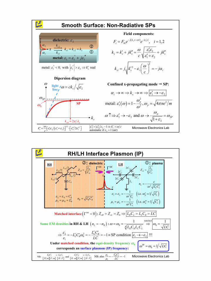
Smooth Surface: Non-Radiative SPsField components:

( )0 , 1, 2ix zj k x t

i iF F e e iαω −− −= =

1 2i xkα ε ε′→∞⇒ →∞⇒ →−

1 2

1 2x x x xk k jk jk

cω ε ε

ε ε′

′ ′′ ′′= + = +′ +

22

zi x i ik j k jcωε α ′= − = −

Confined x-propagating mode SP:

( )2

21 2metal: 1 , 4p

p ne mω

ε ω ω πω

′ = − =

1 22

and 1

pSP

ωω ε ε ω ω

ε′↑⇒ →− → =

+

1 1 2metal: 0, with realxkε ε ε′ ′ ′< > ⇒

metal: 1 1 1jε ε ε′ ′′= +

dielectric: 2ε

x

z

1xk

2xk1 2x x xk k k= =

1α

2α

2xckω ε=

SPω

xk

ω

SP

lightline

0 2x pk π λ=

0ω

Dipersion diagram

( ) 3 2 21 2 1 2 1 12xk c

ω ε ε ε ε ε ε′′ ′ ′ ′′ ′ = + ⋅ 1 1 2

2

1automatic if 1 (air)

xk cε ε ε ωε

′ ′ ′> − ⇒ >=


RH/LH Interface Plasmon (IP)

0cR cL R L L RZ Z Z L C L C LC= = ⇒ = =Matched interface :( )int 0Γ =

220 1 2

1

1 SP condition !!!L RL R

L CL CLC

ε ω ε εε

′ ′′ ′⇒ = − = − = − ≡ → −

Same EM densities in RH & LH :matched

0 04

1 1

R R L LL C L C LCω ω ω= = ⇒ =( )L Rn n= −

Under matched condition, the equi-density frequency ω0corresponds an surface plasmon (IP) frequency:

IP0 1 LCω ω= =

RH LH

RC

2RL

2RL2RL

2RLR

cRR

LZC

=

LL

2 LC2 LC

2 LC2 LC

LcL

L

LZC

=

2

2

R R

R R

CL

ε εµ µ

′= =′= =

( )( )

1 2

1 2

1 i.e. 1

1 i.e. 1

eL p L

Lm

L p LL

LL

CC

ε ε ωω

µ µ ωω

′= = − =′

′= = − =′

: plasma: dielectricintΓ intΓ

R R Rn L C′ ′=

2LL L

cnL Cω

= −′ ′x

z

[ ][ ] [ ] [ ][ ] [ ]NB: and R L R L L R L RL C L C L C L CH m F m H F H m F m H F

′ ′ ′ ′= =⋅ ⋅ ⋅ ⋅

2

1

NB: also 1R LL CLC

µµ

′ ′= − = −

8


Difference Conventional SP and RH/LH-SP

RH/LHRH LHx

z

( )

( )

( )( )

2

1 1 1 12

2 2

TM 1 2

1 2

2TM TM TM2

TM1 2

2

0 and 0 : 1 and 1

cste 0 and cste 0

small : 0 , or

large (SP) : 1

p

x

x x x

px SP

kc

k k ckc

k

ωε µ ε µ

ωε µ

ω ε εε ε

ω εω ω ε

ωε ε ω ω

ε

∗

∗

> = − =

= > = >

=+

→ = =

→ − ⇒ = =+

<

conventionaldielectric metalx

z

2xckω ε=

SPω

xk

ω

SP

lightline

loosely bound

tightly bound

pω

non-radiativeSP

radiativeSP

SP gap

Rexk

RexkImxk

( ) ( )

( )

( )

( )

( )

1 1 1 12 2

2 2

1 2 1 2 2 1TM2 22 1

TM TM

TM1 2

1 10 and 0 : and

and

small : 0

1 1 large (SP) :

L L

R R

x

R Rx x L R

L L

x SPR L

L CC L

kc

C Lk k j L CC L

kL C LC

ε µ ε µω ω

ε µ

ε ε µ ε µ εωε ε

ω

ε ε ω ω

∗ ∗∗

∗

= − = −′ ′

′ ′= =

−=

−

′ ′′ ′→ = + ′ ′

→ ± ⇒ = = =′

<

′

<

SPω

xk

ω

SP

lightline

2xckω ε=

Rexk

Imxk

tightly bound

loosely bound

non-radiativeSP

radiativeSP


Dispersion Diagram of a RH/LH SP

case 1: perfect matching @ ω0

( )

1 2 1 2

B.H.1 2 1 2 2 1

1 12 22 1

and

1x

L L

kc c L C

ε ε µ µ

ε ε µ ε µ εω ω ε µε ε ω

= − = −

⇓

−= → = −

− ′ ′

case 2: small mismatch @ ω0 ( Γ = -30 dB)

case 2: larger mismatch @ ω0 ( Γ = -15 dB) case 2: very large mismatch @ ω0 ( Γ = -3 dB)

SPω

xk

ω

SPω

xk

ω

SPω

xk

ω

( )1 2 1 2 2 12 22 1

xk cε ε µ ε µ εω

ε ε−

=−

Dispersion of LH only !SP radiative and non-radiative

SP essentially non-radiative SP non-radiative

9


Interface Plasmon at a RH/LH 2D-TL Interface

mag

nitu

deph

ase

Voltage distribution @ f = f0 = f IP = 2.826 GHz

RH LH

zRk zLk

xk

xkz

x

RH LH

zRk zLk

xk

xk LR φφ ∆=∆z

x

( )0 : L R L Rn nω ω β β= = − = −

0ω

β

ω

RβLβ

LH RH

R R RL Cβ ω ′ ′=

1L

L LL Cβ

ω= −

′ ′

plasmon frequencyRH LH

RC

2RL

2RL2RL

2RL

LL

2 LC2 LC

2 LC2 LC

zx

zRk zLk

xk

xk

1SP LC

ω =

xk

ωlightline

2xckω ε=

Rexk

Imxk

non-radiativeSP

radiativeSP

Dispersion Diagram

L Rβ β≅ −


Power Distributions of Interface Plasmon

Source(much smallerthan plasmon)

Power along x-direction

Power along z-direction

x

z

x

z

10


Plasmons in Waveguides ConfigurationsFull-Wave FEM (Ansoft-HFSS) simulations of the

WR-650 rectangular waveguide (6.5 3.25’, fc= 0.908GHz)loaded by an ideal LH material,

below cutoff operation: f = 0.85GHz (f< fc)

RH

LH

RH

E-field

z

RH

LH

RH

H-field

z

RH: 1LH: 1

r r

r r

ε µε µ

= = += = −

z

surface plasmons in super-lens

0 a+a− 2a+2a−


Backfire-to-Endfire Leaky-Wave Antenna: ResultsAntenna

Configuration

x

z

ysource

bwd

fwd

broadside

θ

-30

-20

-10

0

0

30

6090

120

150

180

210

240270

300

330

-30

-20

-10

0

f<f0 f=f0 f>f0

RadiationPatterns

ωω

2 3 4 5 6 7-90

-60

-30

0

30

60

90

Scan

ning

Ang

le (d

eg)

Frequency (GHz)

II.LW-LH

III.LW-RH

0f0 2c β π maxf

x y

z

θ

θ versus ω

I.Guided

-LH

2 3 4 5 6 7-4

-3

-2

-1

0

1

2

β / k0 α / k0

Frequency (GHz)

β / k

0

0.00

0.02

0.04

0.06

0.08

0.10

0.12α

/ k0

II.LW-LH

III. LW-RH

0f0 2c β π maxfα / β diagram

I. Guided

-LH

11


Single-Element Purely Passive Retro-Reflector

z

x

y

0θ >

RH range 0ω θ∈ ⇒ >

0Z

1Γ = −

incPreflP

incβreflβ

incSreflS0Z

z

x

y

0θ <

LH range 0ω θ∈ ⇒ <

0Z

incP reflP

1Γ = −

incβ reflβ

reflSincS0Z

θ θ

θ θ

short-circuit

matchedload


Arbitrary Reflective Angle LW Reflecto-Director

LOf

Mixer

1f 12 LOff f−=BPFBPF

RF Oscillator

LW Antenna

( )1 1f θ ( )2 2f θ

1β 1β

principle

practical implementationSchottky

diodemixer CRLH antenna

Mixer1

inf ,2

,2 ,1

22

LO m

L

out

LinO O

f fff f

f = +

= + −BPFBPF

Oscillator 1

Mixer2

Oscillator2,2LOf,1LOf

,1inm LOff f= −

IF-Amp.

LW Antenna

( )in inf θ ( )out outf θ

inβ outβ

,1

,1,2

if is fixed, then

2ou

L

t

O

OL

i LO

n

ff

fff

⇓

− +=

12


Reflector Array of CRLH-TLs Terminated by Shorts

Array Alternating Stub CRLH-TLs

-25

-20

-15

-10

-5

0

0

30

60

90

120

150

180-25

-20

-15

-10

-5

0

3.3 GHz 3.5 GHz 3.7 GHz 4.3 GHz

Mono-Static RCS

Frequency-Scanning observedBackward retrodirectivity observedSpecular reflection (GP) can be removedby using a reference PEC reflectorSpecular reflection may be minimized byetching appropriate slots in the GP

ω θ

Motivations• Larger RCS than single-element reflector• Real surface, possibly conformal to any geometry• Simple and cheap with conv. photolithography• Can include cheap/simple passive mixers for arbitrary angle


Potential Future Applications of Focus / LW / SPLeaky-Wave Full-ScanningSurface Antenna/Reflector

Surface Plasmon Antennas

Pre-Focus Radiation

RH LH

virtual focus

radiationaperture

aperture size (directivity) can be modulated by varying focal length

2D-LW structure

EndfireDispersion Diagram

1SP LC

ω =

xk

ωlightline

2xckω ε=

Rexk

Imxk

non-radiativeSP

radiativeSP

L Rβ β≅ −

Broadside

RH

LH

RH

LH

Date post:	05-May-2018
Category:	Documents
Upload:	tranhanh
View:	229 times
Download:	2 times

New Metamaterials (MMs) based on an Extended...

Documents