Jafari, H., et al.: New Method for Solving a Class of Fractional Partial Differential Equations... THERMAL SCIENCE: Year 2018, Vol. 22, Suppl. 1, pp. S277-S286 S277

NEW METHOD FOR SOLVING A CLASS OF FRACTIONAL PARTIAL DIFFERENTIAL EQUATIONS WITH APPLICATIONS

by

Hossein JAFARI a,b* and Haleh TAJADODI ca Department of Mathematical Sciences, University of South Africa, Pretoria, South Africa

b Department of Mathematics, University of Mazandaran, Babolsar, Iran c Department of Mathematics, University of Sistan and Baluchestan, Zahedan, Iran

Original scientific paper https://doi.org/10.2298/TSCI170707031J

In this work we suggest a numerical approach based on the B-spline polynomial to obtain the solution of linear fractional partial differential equations. We find the operational matrix for fractional integration and then we convert the main prob-lem into a system of linear algebraic equations by using this matrix. Examples are provided to show the simplicity of our method.Key words: fractional partial differential equations, linear B-spline function,

operational matrix, Caputo derivative

Introduction

Over the last decades fractional calculus were not useful application in physics and mathematical, albeit having a long history. In recent years a number of books [1-5] on fractional calculus were published.

Compared with ODE, fractional order differential equations (FDE) has arbitrary or-der derivatives and integrals. Our purpose is essentially useing the linear B-spline functions to solve PDE in fractional calculus. We paid attention on the following a class of fractional PDE (FPDE):

( , ), 0 , 1γ µ

γ µ µ γ∂ ∂+ = < ≤

∂ ∂z z k x t

x t (1)

s.t

0 1 0 2| ( ), | ( )ψ ψ= =

∂ ∂= =

∂ ∂x tz zt xt x

(2)

1 2(0, ) ( ), ( ,0) ( )η η= =z t t z x x (3)

where 1 2 1 2, , , ,ψ ψ η ηk are the known function and ( , )z x t are the unknown functions. The /γ γ∂ ∂z x and /µ µ∂ ∂z t are the fractional Caputo derivative that is given:

( )

( , ) , ( 1, ),( , )

( , ),

mm

m

m

z x tI m m mz x tx

xz x t m

γγ

γ

γ

γ

− ∂∈ − ∈Ν∂ = ∂

∂ =

(4)

* Corresponding author, e-mail: jafari.usern@gmail.com

Jafari, H., et al.: New Method for Solving a Class of Fractional Partial Differential Equations... S278 THERMAL SCIENCE: Year 2018, Vol. 22, Suppl. 1, pp. S277-S286

Note that:

10

1 ( , )( , ) d , 0, 0( ) ( )

x

xz tI z x t x

xγ

γ

τ τ γγ τ −= > >

Γ −∫ (5)

( 1) , 0, 0, 1(1 )

x x xx

γ δδ γ

γ

δ δ µδ γ

−∂ Γ += > > > −

∂ Γ + − (6)

1

0

( , ) (0 , )( , ) , 1!

j jm

x jj

z x t z t xI z x t m mx x j

γγ

γ γ+−

=

∂ ∂= − − < ≤

∂ ∂∑ (7)

where γI is Riemann-Liouville integral operator. There are numerous methods to solve FPDE. These methods include Adomian decomposition method [6], Fractional subequation meth-od [7], homotopy perturbation method [8], collocation method [9] , homotopy analysis method [10], He’s variational iteration method [11], and other methods [12-17].

In the current paper, we suggest the linear B-spline operational matrix method to solve the FPDE. At the first, we approximate z in the eq. (1) by linear B-spline functions of unknown coefficients. Then using operational matrixes, the eq. (1) convert to a set of algebraic equations. Recently, FPDE have been solveing using Linear B-splines operational matrix of fractional derivatives and B-spline wavelet collocation method [14, 18]. Also Haar wavelet method used to sole these equations [19, 20].

The B-spline function and operational matrixes for fractional integration

Linear B-spline function on [0,1] The mth order cardinal B-spline ( )mN x has the knote sequence { , 1,0,1, }− Also

there are polynomials of order m (degree 1−m ) between the knots. The B-spline functions for 2≥m on [0,1] has the following form:

1

0

1( ) ( 1) ( )( 1)!

−+

=

= − − −

∑m

k mm

k

mN x x k

km (8)

where supp[ ( )] [0, ]=mN x m and for 1=m the characteristic function is 1 [0,1]( ) ( )χ=N x x . Here, we apply the linear B-spline function of order 2 in the following form [21]:

2

20

, [0,1),2

( ) ( 1) ( ) 2 , [1,2),0, otherwise

+=

∈ = − − = − ∈

∑ k

k

x xN x x k x x

k (9)

Let , 2( ) (2 ), ,= − ∈jj kN x N x k k j Z and , ( ) =j kB x supp , ,[ ] close{ : 0}= ≠j k j kN x N .

It can show that their support is:

, [2 ,2 (2 )], ,− −= + ∈j jj kB k k k j Z (10)

Define the set of indices:

,{ : [0,1] 0}= ∩ ≠j j kS k B

According to eqs. (9) and (10), the minimum and maximum of { }jS are –1 and 2 1−j . Because support of ,j kN can be outside of [0,1], so we have to define ,φ j k on [0,1]:

Jafari, H., et al.: New Method for Solving a Class of Fractional Partial Differential Equations... THERMAL SCIENCE: Year 2018, Vol. 22, Suppl. 1, pp. S277-S286 S279

, , [0,1]( ) ( ),φ χ= ∈j k j kN x x j Z (11)

The function approximation

We can expand function ( )f x by ,φ j k for a fixed =j J :

2 1

,1

( ) ( ) ( )φ−

=−

≈ = Φ∑J

Tk J k J

kf x c x C x (12)

where the vectors C and Φ J are:

11 0 2[ , , , ]−−= J

TC c c c (13)

1, 1 ,0 ,2( ) [ ( ), ( ), , ( )]φ φ φ −−Φ = J

TJ J J J

x x x x (14)

with

1

1

0

( ) ( )d − = Φ ∫T T

JC f x x x P (15)

and symmetric matrix is given:

1

20

(2 1) (2 1)

1 112 241 1 124 6 241( ) ( )d

21 1 124 6 24

1 124 12

−

+ × +

= Φ Φ =

∫

J J

TJ J JP x x x (16)

Also any function ( , )f x t could expand by linear B-spline functions:

2 1 2 1

, ,1 1

( , ) ( ) ( ) ( ) ( )J J

Tik J i J k J J

i kf x t f x t x F tφ φ

− −

=− =−

≈ ≈ Φ Φ∑ ∑ (17)

where , , ,( ), ( , ), ( )φ φ= ⟨ ⟨ ⟩⟩i k J i J kf x f x t t .

Operational matrix for γIIntegration of the vector Φ J , leads to:

( ) ( ),γ γΦ ≈ Ι Φx J JI x x (18)

where γΙ is the (2 1) (2 1)+ × +J J operational matrix of fractional integration. We obtain the matrix γΙ :

1 1

1

0 0

( ) ( )d ( ) ( )dγ γ γΙ − = Φ Φ = Φ Φ

∫ ∫

T Tx J J x J JI x x x I x x x P (19)

Jafari, H., et al.: New Method for Solving a Class of Fractional Partial Differential Equations... S280 THERMAL SCIENCE: Year 2018, Vol. 22, Suppl. 1, pp. S277-S286

where

1

0

( ) ( )dγ= Φ Φ∫ Tx J JE I x x x (20)

In eq. (20), ,[ ]= i kE a is a (2 1) (2 1)+ × +J J matrix:

1

, , ,0

( ) ( )d , , 1 ,2 1γφ φ= = − −∫

Ji k x J k J ia I x x x i k (21)

and , ( )γφx J kI x according eq. (11) can be obtain:

2

,0

2 1

0

1

11

1

2( ) ( 1) 2 ( )

22 ( 1) 2 ( )(2 )

0, ,2

1(2 ) , ,2 2 21 2(2 ) (2 ) 2 2 ( 1) ,

2 2

(2 ) 2

x xi J

J ki

Ji J

i

J

JJ J J

J JJ J

J

I x I x k ii

x k ii

kx

k kx k x

k kx k x k x

x k

γ γ

γ γ

γγ

γγ

γ

φ

γ

γ

+=

−+

+=

+−

++

+

= − − + = = − − + = Γ +

<

+− ≤ <

=+ +Γ + − − − + ≤ <

− −

∑

∑

1 1 22 ( 1) 2 ( 2) ,2

J JJ

kx k x k xγ γ+ +

+ − + + − + ≤

(22)

So that , 1( )γφ −x JI x and ,2 1

( )γφ−x JJ

I x obtain:

1

, 11 1

1( 1)(2 ) (2 ) ,2 2( )1( 2) ( 1)(2 ) (2 ) (2 1) ,2

J JJ J

x JJ J J

J

x x xI x

x x x x

γ γγ

γ

γ γ γ

γφ

γ γ

+−

−+ +

+ − <= Γ + + − + − ≤

(23)

1,2 1

1 1

2 10,2

2 2 1 1( ) (2 2 1) ,( 2) 2 2

(2 2 1) (2 2 ) (2 2 1) , 1

J

J

J

J JJ J

x J JJ

J J J J J J

x

I x x x

x x x x

γγ γ

γ γ γ

φγ

γ

−+

−

+ +

−<

−= − + ≤ <Γ +

− + − − − + + ≤

(24)

by substituting , ( ), 1, ,2 1γϕ = − −

Jx J kI x k in eq. (21), we can find matrix E:

Jafari, H., et al.: New Method for Solving a Class of Fractional Partial Differential Equations... THERMAL SCIENCE: Year 2018, Vol. 22, Suppl. 1, pp. S277-S286 S281

1 2 3 2 2 1

1 2 2 1 2

1 2 2 2 2 1( 1)

1 2 3

1 2

1 (2 1) (2 1)

10 1

2 0( 4)

0 00 0 0 10 0 0 0 1

γ

κ κ κ κ κµ µ µ κ

µ µ µ κ

γµ µ κ

µ κκ

+

−

− −− +

+ × +

= Γ +

J J

J J

J J

J J

J

E (25)

where

[ ] [ ][ ]

21 2

3 2 22

2

3 2 2 12 1

3 3 51 2

32

2, ( 1)2 2 3( 1) 3( 1) 2 3( 1) ( 1)

( 1) ( 2) , 1, ,2 2

(2 2) 2( 2 4)(2 1) ( 2 1) 3 5 4.2 (2 )

2 4, 3 2 6( 2) 4

J

i

J

J J J J J J

i

i i i i i

i i i

k

i

γ

γ γ γ

γ

γ γ γ

γ γ γ

γ

κ γ κ γ γ

κ γ γ

γ

γ γ γ

µ µ

κ

+

+ + ++

+

+ + ++

+ + +

++

= + = + − −

= − + − − − − − + +

+ − − + = −

= − + − + − + − + + + −

= − = − +

= + −

3 3 3 3( 1) 6 4( 1) ( 2) , 2, ,2 2Ji i i i iγ γ γ γ+ + + ++ + − − + − = −

Numerical solution of FPDE

Consider eq. (1) with conditions (2) and (3). First, we expand

2

( ) ( )∂≈ Φ Φ

∂ ∂TJ J

z x Z tx t

then we have:

2

10 2 2

0 0

d | ( ) ( )d ( ) ( ) ( ) ( )ψ ψ=

∂ ∂ ∂= + ≈ Φ Φ + = Φ Ι Φ +

∂ ∂ ∂ ∂∫ ∫t t

T Tt J J J J

z z zt x Z t t x x Z t xx x t x

(26)

2

10 1 1

0 0

d | ( ) ( )d ( ) ( )[ ] ( ) ( )ψ ψ=

∂ ∂ ∂= + ≈ Φ Φ + = Φ Ι Φ +

∂ ∂ ∂ ∂∫ ∫x x

T T Tx J J J J

z z zx x Z t x t x Z t tt x t x

(27)

So unknown function ( , )z x t obtain:

1 12 2

0

( , ) ( )[ ] ( ) ( )d ( )ψ η≈ Φ Ι Ι Φ + +∫x

T TJ Jz x t x Z t s s x (28)

Then we have:

1 1 1 1 1 1

2 2( ) ( ) ( ) ( )[ ] ( ) ( )γ

γγ γ γ

γ ψ ψ− − − −∂ ∂ = ≈ Φ Ι Φ + = Φ Ι Ι Φ + ∂ ∂

T T Tx x J J J J x

z zI I x Z t x x Z t I xx x

(29)

1 1 1 1 1 1

1 1( )[ ] ( ) ( ) ( )[ ] ( ) ( )T T T Tt t J J J J t

z zI I x Z t t x Z t I xt t

µµ

µ µ µµ ψ ψ

− − − −∂ ∂ = ≈ Φ Ι Φ + = Φ Ι Ι Φ + ∂ ∂ (30)

where 1 12 1( , ) ( ) ( )γ µψ ψ− −= +x tg x t I x I t that can be written:

Jafari, H., et al.: New Method for Solving a Class of Fractional Partial Differential Equations... S282 THERMAL SCIENCE: Year 2018, Vol. 22, Suppl. 1, pp. S277-S286

( , ) ( ) ( )≈ Φ ΦTJ Jg x t x G t (31)

and ,[ ]= i jG g is a (2 1) (2 1)+ × +J J matrix. Also we approximate functions ( , )k x t by the linear B-spline basis:

( , ) ( ) ( )≈ Φ ΦTJ Jk x t x K t (32)

Now, by substituting eqs. (29)-(32) into eq. (1), we obtain:

1 1 1 1( )[ ] ( ) ( )[ ] ( ) ( ) ( ) ( ) ( )γ µ− −Φ Ι Ι Φ + Φ Ι Ι Φ + Φ Φ = Φ ΦT T T T T TJ J J J J J J Jx Z t x Z t x G t x K t (33)

or

{ }1 1 1 1( ) [ ] [ ] ( ) 0γ µ− −Φ Ι Ι + Ι Ι + − Φ =T T TJ Jx Z Z G K t (34)

Finally, eq. (33) give linear system of algebraic equations in the following form:

1 1 1 1[ ] [ ] 0γ µ− −+ + − =T TI ZI I ZI G K (35)

So Z can be computed by solving previous system. Consequently, we get the numeri-cal solution of ( , )z x t using eq. (28).

Numerical examples

Now we solve four examples that shows the efficiency of our technique.Example 1. Analyze the following FPDE [19]:

( )

1/4 1/4 3/4 3/4

1/4 1/4

4( ) , , [0,1]3 3/4

∂ ∂ ++ = ∈

∂ ∂ Γz z x t xt x t

x t (36)

subject to:

0 0| 0, | 0= =

∂ ∂= =

∂ ∂x tz zt x

(37)

(0, ) 0, ( ,0) 0= =z t z x (38)

That exact solution is xt which is studied by Wang et al. [19] by using Haar wavelet. Here we applied the linear B-spline function to solve it. By using eqs. (26) and (27), we have:

2

10

0 0

d | ( ) ( )d ( ) ( )=

∂ ∂ ∂= + ≈ Φ Φ = Φ Ι Φ

∂ ∂ ∂ ∂∫ ∫t t

T Tt J J J J

z z zt x Z t t x Z tx x t x

(39)

2

10

0 0

d | ( ) ( )d ( )[ ] ( )=

∂ ∂ ∂= + ≈ Φ Φ = Φ Ι Φ

∂ ∂ ∂ ∂∫ ∫x x

T T Tx J J J J

z z zx x Z t x x Z tt x t t

(40)

So unknown function ( , )z x t obtain:

1 1 1 1( , ) ( )[ ] ( ) (0, ) ( )[ ] ( )≈ Φ Ι Ι Φ + = Φ Ι Ι ΦT T T TJ J J Jz x t x Z t z t x Z t (41)

According eqs. (29) and (30), we have:

1/4 3/4 3/4 1 3/4 1

1/4 [ ( ) ( )] ( )[ ] ( )T T Tx x J J J J

z zI I x Z t x Z tx x∂ ∂

= ≈ Φ Ι Φ = Φ Ι Ι Φ∂ ∂

(42)

Jafari, H., et al.: New Method for Solving a Class of Fractional Partial Differential Equations... THERMAL SCIENCE: Year 2018, Vol. 22, Suppl. 1, pp. S277-S286 S283

1/4 3/4 1/4 1 1 3/4

1/4 { ( )[ ] ( )} ( )[ ] ( )T T T Tt t J J J J

z zI I x Z t x Z tt t∂ ∂

= ≈ Φ Ι Φ = Φ Ι Ι Φ∂ ∂

(43)

Similarly we approximate 3/4 3/44( )/3 (3/4)+ Γx t xt :

( )

3/4 3/44( ) ( ) ( )3 3/4

+≈ Φ Φ

ΓTJ J

x t xt x K t (44)

and ,[ ]= i jK k is a (2 1) (2 1)+ × +J J matrix. Now by substituting eqs. (42)-(44) into eq. (36), we have:

3/4 1 1 3/4( )[ ] ( ) ( )[ ] ( ) ( ) ( )Φ Ι Ι Φ + Φ Ι Ι Φ = Φ ΦT T T T TJ J J J J Jx Z t x Z t x K t , (45)

or

3/4 1 1 3/4( ){[ ] [ ] } ( ) 0T T TJ Jx ZI Z K tΦ Ι + Ι Ι − Φ = (46)

Finally, we obtain:

3/4 1 1 3/4[ ] [ ] 0Ι Ι + Ι Ι − =T TZ Z K (47)

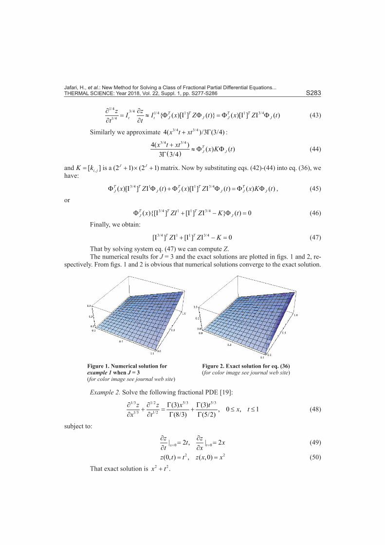
That by solving system eq. (47) we can compute Z. The numerical results for J = 3 and the exact solutions are plotted in figs. 1 and 2, re-

spectively. From figs. 1 and 2 is obvious that numerical solutions converge to the exact solution.

Figure 1. Numerical solution for example 1 when J = 3 (for color image see journal web site)

Figure 2. Exact solution for eq. (36) (for color image see journal web site)

Example 2. Solve the following fractional PDE [19]:

1/3 1/2 5/3 5/3

1/3 1/2

(3) (3) , 0 , 1(8/3) (5/2)

∂ ∂ Γ Γ+ = + ≤ ≤

∂ ∂ Γ Γz z x t x t

x t (48)

subject to:

0 0| 2 , | 2= =

∂ ∂= =

∂ ∂x tz zt xt x

(49)

2 2(0, ) , ( ,0)= =z t t z x x (50)

That exact solution is 2 2 .+x t

Jafari, H., et al.: New Method for Solving a Class of Fractional Partial Differential Equations... S284 THERMAL SCIENCE: Year 2018, Vol. 22, Suppl. 1, pp. S277-S286

This example is studied by Wang et al. [19] using Haar wavelet. Here we applied the linear B-spline function to solve it. Let 2 / ( ) ( )∂ ∂ ∂ ≈ Φ ΦT

J Jz x t x Z t then by using eqs. (26) and (27), we have:

2

10 0

0 0

d | ( ) ( )d | ( ) ( ) 2= =

∂ ∂ ∂ ∂= + ≈ Φ Φ + = Φ Ι Φ +

∂ ∂ ∂ ∂ ∂∫ ∫t t

T Tt J J t J J

z z z zt x Z t t x Z t xx x t x x

(51)

2

10 0

0 0

d | ( ) ( )d | ( )[ ] ( ) 2= =

∂ ∂ ∂ ∂= + ≈ Φ Φ + = Φ Ι Φ +

∂ ∂ ∂ ∂ ∂∫ ∫x x

T T Tx J J x J J

z z z zx x Z t x x Z t tt x t t t

(52)

So unknown function ( , )z x t obtain:

1 1 2 1 1 2 2( , ) ( )[ ] ( ) (0, ) ( )[ ] ( )≈ Φ Ι Ι Φ + + = Φ Ι Ι Φ + +T T T TJ J J Jz x t x Z t x z t x Z t x t (53)

Then

2/3

1/32/3 1 2/3 1 5/3

1/3

2 (2)[ ( ) ( ) 2 ] ( )[ ] ( )(8/3)

T T Tx x J J J J

z zI I x Z t x x Z t xx x∂ ∂ Γ

= ≈ Φ Ι Φ + = Φ Ι Ι Φ +∂ ∂ Γ

(54)

1/2 1/2 1/2 1 1 1/2 3/2

1/2

2 (2){ ( )[ ] ( ) 2 } ( )[ ] ( )(5/2)

T T T Tt t J J J J

z zI I x Z t t x Z t tt t∂ ∂ Γ

= ≈ Φ Ι Φ + = Φ Ι Ι Φ +∂ ∂ Γ

(55)

Substituting eqs. (54) and (55) into eq. (48), we have:

2/3 1 1 1/2( )[ ] ( ) ( )[ ] ( ) 0Φ Ι Ι Φ + Φ Ι Ι Φ =T T T TJ J J Jx Z t x Z t (56)

Finally, we obtain:

2/3 1 1 1/2[ ] [ ] 0Ι Ι + Ι Ι =T TZ Z (57)

So by solving previous system we achieve 0=z . Consequently by substituting 0=z in eq. (53), we obtain the exact solution of eq. (48) that is 2 2( , ) .= +z x t x t

Example 3. Now we examine the numerical solution of the FPDE [19]:

2 2 2 2(3) ( 1) (3)( 1) , 0 , 1(3 ) (3 )

γ µ γ µ

γ µ γ µ

− −∂ ∂ Γ + Γ ++ = + ≤ ≤

∂ ∂ Γ − Γ −z z x t x t x t

x t (58)

subject to:

0 0| 2 , | 2= =

∂ ∂= =

∂ ∂x tz zt xt x

(59)

2 2(0, ) 1, ( ,0) 1= + = +z t t z x x (60)

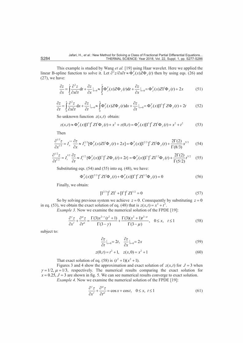
That exact solution of eq. (58) is 2 2( 1)( 1).+ +t xFigures 3 and 4 show the approximation and exact solution of ( , )z x t for 3=J when

1/2, 1/3γ µ= = , respectively. The numerical results comparing the exact solution for 0.25, 3= =x J are shown in fig. 5. We can see numerical results converge to exact solution.

Example 4. Now we examine the numerical solution of the FPDE [19]:

cos cos , 0 , 1z z x t x tx t

γ µ

γ µ

∂ ∂+ = + ≤ ≤

∂ ∂ (61)

Jafari, H., et al.: New Method for Solving a Class of Fractional Partial Differential Equations... THERMAL SCIENCE: Year 2018, Vol. 22, Suppl. 1, pp. S277-S286 S285

subject to:

0 0| cos , | cos= =

∂ ∂= =

∂ ∂x tz zt xt x

(62)

(0, ) sin , ( ,0) sin= =z t t z x x (63)

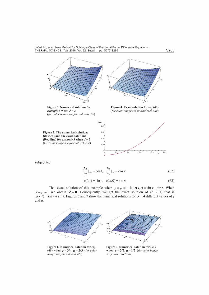
That exact solution of this example when 1γ µ= = is ( , ) sin sin= +z x t x t . When 1γ µ= = we obtain 0=Z . Consequently, we get the exact solution of eq. (61) that is

( , ) sin sin= +z x t x t . Figures 6 and 7 show the numerical solutions for 4=J different values of γ and μ.

Figure 3. Numerical solution for example 3 when J = 3 (for color image see journal web site)

Figure 4. Exact solution for eq. (48) (for color image see journal web site)

z(x,t)

t

Figure 5. The numerical solution: (dashed) and the exact solution: (Red line) for example 3 when J = 3 (for color image see journal web site)

Figure 6. Numerical solution for eq. (61) when = =3/4, 2/3γ µ (for color image see journal web site)

Figure 7. Numerical solution for (61) when = =3/5, 1/3γ µ (for color image see journal web site)

Jafari, H., et al.: New Method for Solving a Class of Fractional Partial Differential Equations... S286 THERMAL SCIENCE: Year 2018, Vol. 22, Suppl. 1, pp. S277-S286

Conclusion

In the present paper we used operational matrix of fractional integration based on lin-ear B-spline function to solve the FPDE. We expand the unknown function with chosen polyno-mial. The problem has been reduced to a system of algebraic equations. Application examples show good coincidence of the numerical result with exact solution. We used Mathematica for computations.

References[1] Gorenflo, R., et al., Fractional Calculus and Continuous-Time Finance, III. the Diffusion Limit, in: Math-

ematical Finance, Trends Math., (Eds., K., Tang) 2001, pp. 171-180[2] Jafari, H., An Introduction to Fractional Differential Equations, (in Persian), Mazandaran University

Press, Babolsar, Iran, 2013[3] Kilbas, A. A., et al., Theory and Application of Fractional Differential Equations, Elsevier, Amsterdam, The

Netherland, 2006[4] Podlubny, I., Fractional Differential Equations, Academic Press, New York, USA, 1999[5] Samko, S., et al., Fractional Integrals and Derivatives: Theory and Applications, Gordon and Breach

Science Publishers, Yverdon, Switzerland, 1993[6] Jafari, H., et al., A Decomposition Method for Solving the Fractional Davey-Stewartson Equations, Inter-

national Journal of Applied and Computational Mathematics, 1 (2015), 4, pp. 559-568[7] Jafari, H., et al., Application of a Homogeneous Balance Method to Exact Solutions of Nonlinear Frac-

tional Evolution Equations, Journal of Computational and Nonlinear Dynamics, 9 (2014), 2, 021019[8] Jafari, H., Momani, S., Solving Fractional Diffusion and Wave Equations by Modified Homotopy Pertur-

bation Method, Phys Lett A, 370 (2007), 5-6, pp. 388-396[9] Tian, W., Polynomial Spectral Collocation Method for Space Fractional Advection-Diffusion Equation,

Numerical Methods for Partial Differential Equations, 30 (2014), 2, pp. 514-535[10] Jafari, H., et al., Homotopy Analysis Method for Solving Abel Differential Equation of Fractional Order,

Central European Journal of Physics, 11 (2013), 10, pp. 1523-1527[11] Jafari, H., et al., Solutions of the Fractional Davey-Stewartson Equations with Variational Iteration Meth-

od, Romanian Reports In Physics, 64 (2012), 2, pp. 337-346[12] Huang, Q., et al., A Finite Element Solution for the Fractional Advection-Dispersion Equation, Advances

in Water Resources, 31 (2008), 12, pp. 1578-1589[13] Momani, S. Odibat, Z., Generalized Differential Transform Method for Solving a Space and Time Frac-

tional Diffusion-Wave Equation, Physics Letters A, 370 (2007), 5-6, pp. 379-387[14] Li, X., Numerical Solution of Fractional Differential Eqiations Using Cubic B-Spline Wavelet Collocation

Method, Commun Nonlinear Sci Numer Simulat, 17 (2012), 10, pp. 3934-3946[15] Lotfi, A., et al., A Numerical Technique for Solving Fractional Optimal Control Problems, Comput. Math.

Appl,. 62 (2011), 3, pp. 1055-1067[16] Rostamy, D., et al., Solving Multi-Term Orders Fractional Differential Equations by Operational Matrices

of BPs with Convergence Analysis, Romanian Reports in Physics, 65 (2013), 2, pp. 334-349[17] Saadatmandi, A., Dehghan, M., A New Operational Matrix for Solving Fractional-Order Differential

Equations, Computers and Mathematics with Applications, 59 (2010), 3, pp. 1326-1336[18] Lakestani, M., et al., The Construction of Operational Matrix of Fractional Derivatives Using B-Spline

Functions, Commun Nonlinear Sci Numer Simulat, 17 (2012), 3, pp. 1149-1162[19] Wang, L., et al., Haar Wavelet Method for Solving Fractional Partial Differential Equations Numerically,

Applied Mathematics and Computation, 227 (2014), Jan., pp. 66-76[20] Wu, J. L., A Wavelet Operational Method for Solving Fractional Partial Differential Equations Numerical-

ly, Applied Mathematics and Computation, 214 (2009), 1, pp. 31-40[21] Boor, C. de, A Practical Guide to Spline, Springer-Verlag, Berlin, 1978

Paper submitted: July 7, 2017Paper revised: December 15, 2017Paper accepted: January 10, 2018

© 2018 Society of Thermal Engineers of SerbiaPublished by the Vinča Institute of Nuclear Sciences, Belgrade, Serbia.

This is an open access article distributed under the CC BY-NC-ND 4.0 terms and conditions