New methodology for calculating damage variables evolution in Plastic Damage Model for RC structures

B. Alfarah1, F. López-Almansa2, S. Oller3

1 PhD Candidate, Technical University of Catalonia, Civil and Environmental Engineering Department, Campus Nord UPC, 08034 Barcelona, Spain

2 Professor, Technical University of Catalonia, Architecture Technology Department, Avda. Diagonal 649, 08028 Barcelona, Spain

3 Professor, Technical University of Catalonia, Civil and Environmental Engineering Department, Campus Nord UPC, 08034 Barcelona, Spain

Correspondence to: Francisco López-Almansa; Departament d’Estructures; ETSAB (UPC); Avda.

Diagonal 649; 08028 Barcelona (Spain); Phone +34934016316, FAX +34934016096; E-mail: francesc.lopez-almansa@upc.edu

Abstract: The behavior of reinforced concrete (RC) structures under severe demands, as strong ground motions, is highly complex; this is mainly due to joint operation of concrete and steel, with several coupled failure modes. Furthermore, given the increasing awareness and concern for the important seismic worldwide risk, new developments have arisen in earthquake engineering. Nonetheless, simplified numerical models are widely used (given their moderate computational cost), and many developments rely mainly on them. The authors have started a long-term research whose final objective is to provide, by using advanced numerical models, solid basis for these developments. Those models are based on continuum mechanics, and consider Plastic Damage Model to simulate concrete behavior. Within this context, this paper presents a new methodology to calculate damage variables evolution; the proposed approach is based in the Lubliner/Lee/Fenves formulation and provides closed-form expressions of the compressive and tensile damage variables in terms of the corresponding strains. This methodology does not require calibration with experimental results and incorporates a strategy to avoid mesh-sensitivity. A particular algorithm, suitable for implementation in Abaqus, is described. Mesh-insensitivity is validated in a simple tension example. Accuracy and reliability are verified by simulating a cyclic experiment on a plain concrete specimen. Two laboratory experiments consisting in pushing until failure two 2-D RC frames are simulated with the proposed approach to investigate its ability to reproduce actual monotonic behavior of RC structures; the obtained results are also compared with the aforementioned simplified models that are commonly employed in earthquake engineering. Keywords: Concrete Plastic Damage Model, Damage variables calculation, Mesh-sensitivity, Numerical simulation, Concrete structures, Seismic behavior.

1. Introduction

Under severe seismic excitation, structural behavior of buildings and other constructions is highly complex. It involves, among other issues, soil-structure interaction, large strains and displacements, damage, plasticity, and near-collapse behavior. Moreover, in reinforced concrete structures, there are several coupled degradation and failure modes: cracking, crushing and spalling of concrete, yielding and pull-out of tensioned reinforcement, and yielding and buckling of compressed reinforcement. Therefore, in earthquake engineering, advanced numerical simulations based on continuum mechanics are strongly necessary; conversely, oversimplified models are commonly used, as a result of their moderate computational cost. Furthermore, another circumstance makes the situation more alarming: given the increasing awareness and concern on the huge worldwide seismic risk, earthquake engineering has experienced in last years substantial advances. New design and analysis strategies have been proposed, leading to relevant developments. These developments rely on extensive testing and numerical simulation; nonetheless, as discussed before, an important number of numerical analyses are mainly conducted by using simplified models. Therefore, there is a strong need of verifying the reliability

2

of the new developments by comparison with analyses performed using more advanced simulation tools. Being aware of this circumstance, the authors have started a long-term research activity aiming to clarify this issue and to provide accurate and reliable models that are based on continuum mechanics. This paper presents early results of this research. Quasi-brittle materials, as concrete, exhibit nonlinear stress-strain response mainly because of micro-cracking. Cracks are oriented as the stress field and generate the failure modes. In tension, failure is localized in a narrow band; stress-strain behavior is characterized by sudden softening accompanied with reduction in the unloading stiffness. In compression, failure begins usually in the outside and is more complex, involving volumetric expansion, strain localization, crushing, inclined slipping and spalling; stress-strain behavior involves ductile hardening followed by softening and reduction in the unloading stiffness. In mixed stress states, failure depends usually on the ratio between the principal stresses; in tension-compression, failure is generated by the compression of the material that is between the cracks. Noticeably, in tension the behavior is closer to damage than to plasticity; conversely, in compression the participation of plasticity is higher. Nonlinear concrete response can be represented using plasticity or damage theory. However, none of these formulations alone is able to describe adequately this phenomenon. Plastic models [Chen, Chen 1975; Lin et al. 1987] might represent realistically the observed deformation in high confined concrete but do not capture the stiffness degradation observed in experiments [Grassl, Jirasek 2006a]. Damage-based models [Mazars 1984; Mazars et al. 1989; Challamel et.al 2005] are based on gradual reduction of the elastic stiffness; they can describe the stiffness degradation in tension and low confined compression, but are not suitable to capture the irreversible deformations observed in experiments and the inelastic volumetric expansion in compression. In addition, fracture propagation can be represented by embedded crack models, where standard FEM interpolations are enriched with strain or displacement discontinuities [Belytschko et al. 1988; Simo, Oliver 1994; Jirásek, Zimmermann 2001]. These models can be used for high strain localization problems (fracture). It is been widely accepted that coupling between damage and plasticity models is essential to capture the nonlinear behaviour of concrete [Nguyen, Korsunsky 2008]. Plasticity for concrete can be described with isotropic hardening; however, damage in many cases is not isotropic but has preferential directions [Fichant et al.1999]. Some plastic isotropic damage models have been proposed, e.g. [Luccioni et al. 1996; Lee, Fenves 1998; Burlion et al.2000; Salari et al. 2004; Krätzig, Pölling 2004; Jason et al. 2006; Grassl, Jirasek 2006a; Nguyen, Korsunsky 2008]; these models have shown good performance in capturing concrete behaviour in tests on full-scale structures [Fichant et al. 1999; Nguyen, Korsunsky 2008]. Anisotropy can be added to the damage to capture the anisotropy feature of concrete both for compression and tension. Although anisotropic damage models are complex and coupling with plasticity in the application to practical engineering is not straightforward, researchers have investigated this issue and proposed plastic anisotropic damage models, among others [Ortiz 1985; Simo, Ju 1987; Ju W 1989; Govindjee et al. 1995; Meschke et al. 1998; Halm, Dragon 1998; Carol et al. 2001; Hansen et al. 2001; Cicekli et al. 2007; Voyiadjis et al. 2008; Al-Rub, Kim 2010]. Even if isotropic damage is a simplified assumption, it is considered in this work because of its simplicity and sufficient accuracy. Coupled damage and plasticity models for concrete differ mainly in the coupling method and the damage evolution law. In the implicit methods [Luccioni et al. 1996; Nguyen, Houlsby 2004; Salari et al. 2004], coupling is embedded in yield and damage criteria; damage evolution law is also implicit. Other researchers describe coupling using a single function. In this context, [Lee, Fenves 1998; Lemaitre 1992] use a yield function; damage measure can be based on some criteria or by postulating damage variables law. This function can be also interpreted as a damage loading [Faria et al. 1998]; the damage evolution law shall be imposed.

3

Damage evolution law plays an important role in any damage model, particularly when this law is imposed. A number of researchers have proposed different damage evolutions laws. Most of them are based on splitting damage into compressive and tensile parts and each one is determined separately by its evolution law; total damage is calculated with some combination rules e.g. [Faria et al. 1998; Britel, Mark 2006; Al-Rub, Kim 2010; López-Almansa et al. 2014]. Few evolution laws are based on general formulae for calculating damage in compression and tension [Häussler et al. 2008]. In most of the available damage evaluating formulae the parameters need to be calibrated experimentally [Mazars et al. 1989; Faria et al. 1998; Britel, Mark 2006; Häussler et al. 2008; Al-Rub, Kim 2010]; other approaches use empirical formulation with some assumptions on stress invariants [Yu et al. 2010] or with iterative procedures aiming to fit experimental results [López-Almansa et al. 2014]. After these investigations, this paper proposes a new approach for obtaining damage variables. The need of proposing a new methodology arises from their advantages: Is based on the formulation by Lubliner and Lee/Fenves [Lubliner et al. 1989; Lee, Fenves

1998], which is the base for the Abaqus plastic damage model for concrete. The proposed approach modifies this formulation and obtains closed-form expressions of the damage variables in terms of the corresponding strains; these expressions are derived after integration of concrete fracture and crushing energy.

No calibration with experimental results is required. Implementation is particularly easy. Results are insensitive of mesh size, since a strategy aiming to avoid mesh-dependency is

incorporated. All these advantages make this methodology well suited for practical applications. Noticeably, the default Abaqus model based on the Lubliner/Lee/Fenves approach requires that the uniaxial damage variables (i.e. the damage evolution) are provided by the user, and no guidelines are provided. Therefore, defining the damage evolution is a big concern for any user of the Concrete Damage Plastic Model. In the proposed model, constant mesh size is required in the elements corresponding to the same material. If elements with different size are employed for a single material, their parameters should be defined individually for each size following the proposed methodology. This approach can consider any concrete constitutive law, either empirical (e.g. like formulations commonly recommended by design codes) or directly based on particular experiments; noticeably, any such constitutive law should account for mesh-sensitivity. In this paper, a particular algorithm that uses laws based on European recommendations is derived; in this case, the only input parameters are concrete compressive strength and mesh size. This algorithm is implemented in the software package Abaqus [Abaqus 2013]; could be also implemented in other computer codes that contain Plastic Damage Model and that require values of damage variables. Mesh-insensitivity of the proposed methodology is validated in a simple tension example. Accuracy and reliability are verified by simulating, with the said particular algorithm, a cyclic experiment on plain concrete specimens. Furthermore, two laboratory experiments are described with the proposed approach to investigate its capability to reproduce the behavior of reinforced concrete (RC) framed structures. These experiments are monotonic pushing tests of 2-D RC frames. Obtained numerical results are also compared with those from simplified models that are most commonly utilized in earthquake engineering research and practice. Noticeably, the objective of this comparison is not to highlight the superior quality of the proposed approach, but to point out that using oversimplified models can led to significant errors.

4

This work considers full bonding between concrete and steel; it is simulated by the “embedded element technique” [Lykidis, Spiliopoulos 2008]. This formulation has proven satisfactory for monotonic behavior of reinforced concrete. Conversely, cyclic comportment of RC structures cannot be adequately reproduced with this assumption, because actual bonding behavior involves sliding, thus leading to pinching effects. For that reason, research aiming to incorporate other formulations for describing bonding is currently in progress. Further long-term research will involve extensive use of the derived models for verification and grounding of commonly used strategies in earthquake engineering and for proposal of new formulations. 2. Concrete Plastic Damage Model

As discussed in the Introduction, the structural behavior of RC structures is highly complex, because the joint operation of concrete and steel. Concrete behavior is brittle, but, under stress reversal, tensile cracks might close, then broken parts being reassembled. Conversely, steel behavior is ductile, with extremely rare fractures, and broken parts cannot be reunited. Therefore, concrete behavior can be better described with damage models, whereas plasticity models better represent steel behavior. Nevertheless, since steel brings additional ductility, the behavior of concrete belonging to reinforced concrete can be even better described with models that combine damage and plasticity. These models are particularly well suited for reproducing failure modes that are based on tensile cracking and compression crushing. In this paper, steel behavior is simulated with a uniaxial plasticity model and concrete is described with a multiaxial model that considers parallel combination of scalar (isotropic) damaged elasticity and non-associated multi-hardening plasticity. This model is termed as “Concrete Plastic Damage Model” (CPDM) along this paper. Was proposed for monotonic, cyclic and dynamic behavior by [Lubliner et al. 1989] and was further developed by [Lee, Fenves 1998]. This model shows good performance in primarily uniaxial and biaxial stress states, but should not be used in case of significant triaxial compressive stresses. Figure 1 displays uniaxial stress-strain plots typical of plasticity, damage and damage-plasticity models; loading branches are represented with solid thick lines and unloading / reloading branches are plotted with dashed thin lines. E0 is the initial (undamaged) elastic stiffness (deformation modulus), and el and pl are the elastic (recoverable) and plastic (irrecoverable) strain, respectively. Figure 1 shows that damage generates stiffness degradation [Oller 2014] since the slope of unloading / reloading branch is (1 d) E0 where d is a damage variable ranging between 0 (no damage) and 1 (destruction).

(a) Plasticity Model (b) Damage Model (c) Plastic Damage

Model

Figure 1. Representation of CPDM For uniaxial compression and tension, the stress-strain relation under uniaxial loading in the damage-plasticity behavior displayed in Figure 1.c, can be written as:

5

σ 1 ε ε (1)

σ 1 ε ε (2)

Subindexes c and t refer to compression and tension, respectively. For uniaxial cyclic loading-unloading conditions, the damage plasticity model assumes that the degradation in the elastic stiffness is given by

1 (3) In equation (3), E is the reduced tangent stiffness and d is a scalar degradation variable, which is a function of stress state and of compression and tension damage variables (dc and dt, respectively):

1 1 1 (4) In equation (4), sc and st are dimensionless coefficients accounting for stress state and stiffness recovery effects, being given by

1 1 ∗ (5) 1 ∗ (6)

In equations (5) and (6), σ is the first principal uniaxial stress (positive for tension), r* is a stress state parameter being ∗ = 1 for tension and ∗ = 0 for compression, and and are weighting factors ranging between 0 and 1. Factor accounts for re-closing of cracks after tension-compression reversal; represents recovery of crushed concrete after compression-tension reversal. In this work, c = 0.9 and t = 0 is assumed; this means that 90% of the cracks close upon tension-compression reversal and the crushed concrete does not experience any recovery. Equations (5) and (6) show that and also range between 0 and 1. For a better understanding of the effect of sc and st coefficients, Figure 2 displays plots of uniaxial stress-strain loading-unloading behavior. The initial elastic branch with slope E0 reaches the descending branch (Figure 5.b) at peak point 1, then cracking begins; later, unloading starts at point 2. At that point, there is no compression damage and dc = 0, r* = 1, and sc = 1; therefore, equation (4) shows that d = dt. Consequently, the linear unloading branch has slope (1 dt) E0. In the way to stress reversing point 3, cracks begin closing. After point 3, r* = 0, sc = 1 hc, st = 1, dc = 0, and equation (4) shows that d = (1 hc) dt. Therefore, the slope of the ongoing compression segment of the branch depends on parameter hc; three options are plotted in Figure 2: (i) hc = 0 (no crack is closed) with slope (1 dt) E0, (ii) hc = 0.5 (half of the cr acks are closed) with slope (1 0.5 dt) E0, (iii) hc = 1 (all cracks are closed) with slope E0. Noticeably, in the third option (hc = 1), there is no compressive strength reduction. At point 4, an unloading branch arises; at that point, r* = 0, sc = 1 hc, st = 1, and equation (4) shows that 1 d = (1 dc) [1 (1 hc) dt] = 1 dc. Point 5 correspond again to stress reversal; after it, provided that ht = 0, the slope of the ongoing branch is equal to (1 dt) (1 dc) E0. Point 6 is the peak for the reduced tensile strength; after it, cracking reinitiates and a new descending branch is generated.

6

Figure 2. Uniaxial loading-unloading law

For multiaxial condition, the stress-strain relationship is given by:

σ 1 D ∶ ε ε (7) In equation (7), D is the elastic stiffness tensor, and σ and ε are the stress and strain tensors, respectively. Scalar damage variable d keeps same meaning than for uniaxial condition, although replacing scalar factor ∗ with a multiaxial one [Lee, Fenves 1998]. Regarding plasticity model, yield condition is based on the loading function F proposed in [Lubliner et al. 1989] with modifications suggested by [Lee, Fenves 1998] to account for different tension and compression strength evolution.

1

1 α3α β⟨σ ⟩ γ⟨ σ ⟩ 0 (8)

α/ 1

2 / 1; β 1 α 1 α ; γ

3 12 1

(9)

In equations (8) and (9), ⟨ ⟩is the Macaulay bracket, is the hydrostatic pressure stress, is the Von Mises-equivalent effective stress (effective stress accounts for stress divided by 1 d), and fb0 and fc0 are the biaxial and uniaxial compressive yield strengths, respectively; since fb0 fc0, ranges between 0 (fb0 = fc0) and 0.5 (fb0 ≫ fc0). σ is the maximum principal effective stress, and and are the effective compressive and tensile cohesion stress, respectively. and are defined as σ / 1 and σ / 1 . Kc is the ratio of second stress invariants on tensile and compressive meridians. The plasticity model assumes non-associated potential plastic flow. The flow potential G is the Drucker-Prager hyperbolic function given by:

ϵσ tanψ tanψ (10)

In equation (10), σt0 is the uniaxial tensile stress at failure, ϵ is the eccentricity of plastic potential surface, and ѱ is the dilatancy angle measured in - (deviatory) plan at high confining pressure. As discussed previously, Kc is the ratio between the magnitudes of deviatoric stress in uniaxial tension and compression; Kc ranges between 0.5 (Rankine yield surface) and 1 (Von Mises). In

7

this study, Kc is obtained from the Mohr-Coulomb yield surface function in cylindrical coordinates [Oller 2014]:

ρ, , θ, ϕ, √2sinϕ √3ρcosθ ρ sin θ sinϕ √6 cosϕ 0 (11) In equation (11), is the octahedral radius, is the distance from the origin of stress space to the stress plan, is the Lode similarity angle, ϕ is the friction angle, and c is the cohesion. In equation

(11), 2 , = I1 / √3, and sin √/ ; I1 is the first invariant of stress tensor and J2 and

J3 are the second and third invariants of deviatoric stress tensor, respectively. For = 0 and θ = π / 6 (negative/positive for tension/compression meridian plans), the magnitudes of deviatory stress in uniaxial compression and tension at yield (ρc0 and ρt0) and Kc are

ρ 2 √6cosϕ3 sinϕ

ρ 2 √6cosϕ3 sinϕ

ρρ

3 sinϕ3 sinϕ

(12)

By assuming that ϕ = 32° [Oller 2014], last equation in (12) shows that Kc = 0.7. Figure 3 represents the yield surface in deviatory plan for several values of Kc ranging from 0.5 to 1. CM and TM account for compression/tension meridian plans, respectively.

Figure 3. Yield surface in the deviatory plan for several values of Kc Equations (10), (8) and (9) show that the concrete behavior depends on four constitutive parameters Kc, ѱ, fb0 / fc0, ϵ; it can be assumed that ѱ =13° [Vermeer, de Borst 1984]. Table 1 describes the values used in this study.

Table 1. Parameters of CPDM Kc Ѱ (º) fb0 / fc0 ϵ 0.7 13 1.16 0.1

3. Proposed Methodology for Calculating Damage Variables

3.1. General description

The proposed approach for calculating the damage variables starts from definition of compressive and tensile variables as the portion of normalized energy dissipated by damage:

8

1

σ dε 1

σ dε (13)

In equation (13), ε and ε are the crushing and cracking strains respectively, see Figure 5. Normalization coefficients gc and gt represent the energies per unit volume dissipated by damage along the entire deterioration process:

σ dε σ dε (14)

Equations (13) and (14) show that dc and dt range between 0 (no damage) and 1 (destruction). Figure 4 describes the meaning of gc and gt.

(a) Compression (gc) (b) Tension (gt)

Figure 4. Parts of energy dissipated by damage Noticeably, the energies per unit area and per unit volume are related by / and / ; and are material parameters defined as crushing and fracture energies and is the characteristic length of the element (subsection 3.2). Relation between compressive and tensile stress and, respectively, crushing and cracking strain, is established, according [Lubliner et al. 1989], as:

1 exp ε exp 2 ε (15)

1 exp ε exp 2 ε (16) In equations (15) and (16), fc0 and ft0 and are the compressive and tensile stresses that correspond to zero crushing (ε 0) and to onset of cracking (ε 0), respectively; see Figure 4. As well, ac, at, bc and bt are dimensionless coefficients to be determined. Replacing equations (15) and (16) in equation (14), provides the following relations among gc and gt and such coefficients:

1

2

1

2 (17)

Coefficients bc and bt can be obtained by replacing / and / in equation (17):

1

2

1

2 (18)

By substituting results (15) through (17) in equation (13), the proposed tensile and compressive damage functions are derived:

9

11

22 1 exp ε exp 2 ε (19)

11

22 1 exp ε exp 2 ε (20)

Therefore, provided that coefficients ac and at are not zero:

exp ε1

1 1 2 (21)

exp ε1

1 1 2 (22)

By zeroing derivatives of c and t (equations (15) and (16), respectively) with respect to, respectively, crushing and cracking strain, maximum values fcm and ftm (Figure 5) are obtained:

14

14

(23)

Equations (23) provide:

a 2 ⁄ 1 2 ⁄ ⁄ (24)

a 2 ⁄ 1 2 ⁄ ⁄ (25) These developments complete the description of the proposed methodology. Parameters ac, at, bc and bt can be determined from equations (24), (25) and (18) in terms of fcm, fc0, ftm, ft0, leq, Gch and GF. Then, the damage functions can be calculated according equations (19) and (20). An implementation of the proposed approach using the concrete behavior described in next subsection is presented in subsection 3.3.

3.2. Uniaxial concrete behavior

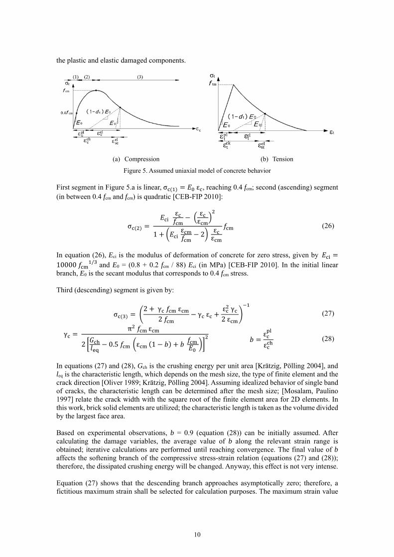
This subsection describes the concrete uniaxial stress-strain law that is selected for implementation. Figure 5.a and Figure 5.b explain the compressive and tensile models, respectively; noticeably, tensile model is smeared, i.e. strain includes both crack opening and actual tensile strain between cracks. Figure 5 displays the constitutive laws (thick solid lines) and the unloading / reloading branches (thin dashed lines). Figure 5 corresponds to the damage-plasticity behavior depicted in Figure 1.c. The ascending compressive segments in Figure 5.a follow the Model Code recommendations [CEB-FIP 2010] and the descending segment is engendered as [Krätzig, Pölling 2004]. Tensile stress-strain relation consists of an initial linear segment and a nonlinear descending branch [Vonk 1993; Van Mier 1984], as shown in Figure 5.b. Both compressive and tensile descending branches are generated to ensure nearly mesh-independency; the regularization approach is based on selecting the softening branches of concrete constitutive laws depending on mesh size. In Figure 5, fcm and ftm represent compressive and tensile stress strength, respectively; corresponding strains are cm and tm, respectively. According to [CEB-FIP 2010], it is assumed that εcm = 0.0022, fcm = fck + 8 (fck is the characteristic

value of concrete compressive strength), and 0.3016 / ; these stresses and the

deformation modulus are expressed in MPa. In Figure 5.a, ε and ε are the crushing and elastic

undamaged components of strain; ε and ε are the plastic and elastic damaged components. In

Figure 5.b, ε and ε are the cracking and elastic undamaged strain components; ε and ε are

10

the plastic and elastic damaged components.

(a) Compression (b) Tension

Figure 5. Assumed uniaxial model of concrete behavior First segment in Figure 5.a is linear,σ ε , reaching 0.4 fcm; second (ascending) segment (in between 0.4 fcm and fcm) is quadratic [CEB-FIP 2010]:

σ ε

εε

1 ε

2 εε

(26)

In equation (26), Eci is the modulus of deformation of concrete for zero stress, given by 10000 / and E0 = (0.8 + 0.2 fcm / 88) Eci (in MPa) [CEB-FIP 2010]. In the initial linear branch, E0 is the secant modulus that corresponds to 0.4 fcm stress. Third (descending) segment is given by:

σ 2 γ ε

2γ ε

ε γ

2ε (27)

γ π ε

2 0.5 ε 1

ε

ε (28)

In equations (27) and (28), Gch is the crushing energy per unit area [Krätzig, Pölling 2004], and leq is the characteristic length, which depends on the mesh size, the type of finite element and the crack direction [Oliver 1989; Krätzig, Pölling 2004]. Assuming idealized behavior of single band of cracks, the characteristic length can be determined after the mesh size; [Mosalam, Paulino 1997] relate the crack width with the square root of the finite element area for 2D elements. In this work, brick solid elements are utilized; the characteristic length is taken as the volume divided by the largest face area. Based on experimental observations, b = 0.9 (equation (28)) can be initially assumed. After calculating the damage variables, the average value of b along the relevant strain range is obtained; iterative calculations are performed until reaching convergence. The final value of b affects the softening branch of the compressive stress-strain relation (equations (27) and (28)); therefore, the dissipated crushing energy will be changed. Anyway, this effect is not very intense. Equation (27) shows that the descending branch approaches asymptotically zero; therefore, a fictitious maximum strain shall be selected for calculation purposes. The maximum strain value

11

shall fulfill that the crushing energy in equation (32) is equal to the area under the corresponding compressive stress-strain law multiplied by the characteristic length. Regarding tensile behavior, the ratio between tensile stress t(w) (for crack width w) and maximum tensile strength ftm, is given by [Hordijk 1992]:

1 e

1 e (29)

In equation (29), c1 = 3, c2 = 6.93 [Hordijk 1992], and wc is the critical crack opening. Equation (29) shows that t(0) = ftm and t(wc) = 0. Therefore, wc can be considered as the fracture crack opening. Equation (30) [Hordijk 1992] relates wc with the tensile strength and fracture energy GF per unit area:

5.14 / (30) According to [CEB-FIP 2010], GF (N/mm) can be calculated as

0.073 . (31)

In equation (31), fcm is expressed in MPa. The ratio between crushing and fracture energies can be assumed proportional to square of the ratio between compressive and tensile strengths [Oller 1988]:

(32)

In this work, the actual crack spacing is not studied, it has been assumed that there is a single crack per element. This supposition is suitable for global-purpose simulation. After this assumption, in the descending segment of the tensile stress-strain curve (Figure 5.b), the strain can be obtained in terms of the crack opening from the following kinematic relation:

ε ε / (33) This subsection describes the concrete uniaxial concrete behavior; next subsection describes their implementation in the proposed approach.

3.3. Implementation

Following the formulation described in the previous section, coefficients ac, at, bc and bt (subsection 3.1) can be determined. Coefficient ac is obtained by replacing fc0 = 0.4 fcm (Figure 5.a) in equation (24). Figure 5.b shows that ftm = ft0, then equation (25) shows that at = 1. Coefficient bc can be determined from equation (18) by replacing fc0 = 0.4 fcm = 0.4 (fck + 8) MPa.

Coefficient bt is determined by replacing at = 1 and 0.3016 / [CEB-FIP 2010] in equation (18). Therefore:

7.873 1 1.97 8

0.453 /

(34)

In the last two expressions in equation (34), fck is expressed in MPa. After parameters ac, at, bc and bt, damage variables dc and dt are determined by equations (19) and (20) in terms of crushing and

12

cracking strain, respectively. A particular implementation of the proposed methodology by using the previously described concrete constitutive law (subsection 3.2) is described next. All stress values are in MPa. 1. The input data are the concrete compressive strength fck, the parameters in Table 1, the mesh

size , and the ratio b (eqn. (28)). Initial assumption is b = 0.9

2. Calculate the compressive / tensile stress strength fcm = fck + 8 / 0.3016 / 3. State the strain at compressive stressstrength as εcm = 0.0022

4. Calculate the initial tangent modulus of deformation of concrete 10000 and the

undamaged modulus of deformation 0.8 0.2

5. Calculate the fracture / crushing energy (N/mm) 0.073 . /

6. Calculate the critical crack opening 5.14 / 7. Build the first / second / third segments of the concrete uniaxial compressive law: σ

ε / eqn. (26) / eqn. (27). In eqn. (27), strain is bounded; the selected upper bound should fulfill the condition that the crushing energy Gch (equation (32)) is reached

8. Build the first / second segment of the concrete uniaxial tensile law: σ ε / eqns. (29) and (33)

9. Calculate the damage parameters according equation (34): 7.873 ; 1 ; .

; . /

10. Calculate the compressive / tensile damage variables (damage evolution) according to eqns. (19) / (20)

11. Calculate the compressive and tensile plastic strains as indicated in Figure 5: ε εσ / 1 , ε ε σ / 1

12. Calculate the average value of ratio and compare with the assumption in step 1.

Repeat until reaching convergence. Once convergence is reached, the major output are curves of compressive / tensile stress and damage variables vs. crushing / cracking strain, respectively; in subsection 3.4, Figure 7 presents some examples. These plots constitute the input of the implementation in any model describing the global structural behavior. This algorithm is suited for software package Abaqus [Abaqus 2013; López-Almansa et al. 2012; Castro et al. 2014]. Noticeably, the proposed approach can be also fitted for other computer codes and for other concrete formulations, either empirical (code-type) or directly based on experiments. Time integration follows an implicit formulation, and the global algorithm is generated by imposing energy balance. In this work, analyses are conducted for large displacements, although not for large strains.

3.4. Mesh-insensitivity verification

When the material exhibits softening, finite element size influences significantly the entire model behavior due to localization since the dissipated energy decreases upon mesh refinement. This can be solved by the so-called mesh regularization techniques. One of the simplest remedy is the Crack Band Method; it uses energy-based scaling of the softening part of the stress-strain relation [Bazant, Oh 1983]. This technique can be considered as a simple and effective method for practical engineering analysis and has been implemented in many concrete plastic damage models,

13

among others [Grassl, Jirasek 2006a; Cicekli et al. 2007]. More advanced techniques are the so-called Non-Local approaches; they are based on introducing non-locality in the constitutive model. This non-locality can be incorporated into an integral format [Bazant et al. 1984; Bazant et al. 1988]; this approach has been implemented in different plastic damage models [Grassl, Jirasek 2006b; Nguyen, Korsunsky 2008]. Another strategy for incorporating non-locality is including higher-order deformation gradients in the model [Peerlings et al. 1998]. This has been implemented in several plastic damage models [Addessi et al. 2002; Al-Rub, Voyiadjis 2009]. As the model of [Lubliner et al. 1989] is the base of this work and this model uses the fracture energy-based regularization to describe the softening in tension and compression, the crack band technique is considered. Then both fracture and crushing energies are scaled in relation to the finite element size. The main assumption in this technique is that damage is localized in a single raw of elements; this is true for the physical failure mechanism of concrete in tension but is not exactly right for compression. Uniaxial compression tests show a great relation between boundary conditions, concrete strength, size, and failure mechanism [Kotsovos 1983, Van Mier, Vonk 1991]. It varies between cone failure and vertical splitting modes. Cone failure occurs when friction at top and bottom sections restraints lateral expansion; this mode is characterized by inclined slip bands at each corner and crushing in the middle zone for very stocky specimens. Vertical splitting mode can happen for highly slender specimens when the effect of friction is neglectable. Intermediate scenarios can occur for different degrees of friction and slenderness; they are characterized mainly by inclined shear band zone. Regarding damage localization under compression, experimental observation by [Kotsovos 1983; Van Mier 1984; Jansen, Shah 1997] showed strain localization; analytical investigation by [Markeset, Hillerborg 1995] showed that the concept of fracture energy in tension holds true for compression. This gives the evidence to use the fracture energy-based regularization in describing the softening of concrete under compression [Van Mier 2013]. In this subsection the capacity of proposed methodology to overcome mesh insensitivity is verified for a uniaxial tension problem. Given the above considerations, it is apparent that the uniaxial compression case cannot be verified in the same way. For practical engineering applications, behavior is mainly controlled by bending and there will be mixed stresses states with high stress gradients; therefore, the possible inaccuracies will have little effect on overall results. This subsection describes the application of the proposed methodology to the problem of uniaxial tension of a 200 mm 200 mm 200 mm cube, as described in Figure 6. The cube is discretized with a uniform mesh of 3D 8-node hexahedron solid finite elements (C3D8R). Figure 6 displays three sketches of the cube discretized with a coarse mesh (leq = 200 mm, one element), a medium mesh (leq = 50 mm, 64 elements) and a fine mesh (leq = 25 mm, 512 elements), respectively. The objective of this analysis is to verify the allegedly low sensitivity to mesh size.

14

(a) Coarse mesh (200 mm) (b) Medium mesh (50 mm) (c) Fine mesh (25 mm)

Figure 6. Uniaxial tension example This problem is analyzed with the algorithm described in subsection 3.2. Table 2 displays the values of the parameters for each mesh size. Any of the values of parameter b in Table 2 is the result of an independent iterative process starting from 0.9. For consistency, the final value is independent on this initial assumption.

Table 2. Parameters for the mesh-insensitivity verification example

Mesh leq

(mm) fck

(MPa) fcm

(MPa) ftm

(MPa) Gch

(N/mm) GF

(N/mm) b ac at bc bt

Coarse 200 25 33 2.58 22.43 0.137 0.6 7.873 1 581 5648 Medium 50 25 33 2.58 22.43 0.137 0.914 7.873 1 145.2 1412

Fine 25 25 33 2.58 22.43 0.137 0.967 7.873 1 72.6 706 The algorithm is implemented in Abaqus code [Abaqus 2013]. The displacement is applied incrementally; for coarse / medium / fine meshes, the maximum number of iterations is 4, 6 and 5, respectively. Figure 7 presents the plots that constitute the major inputs for this implementation. Figure 7.a and Figure 7.b display plots of compressive/tensile stress vs. crushing/cracking strain, respectively; Figure 7.c and Figure 7.d display plots of compressive/tensile damage variable vs. crushing/cracking strain, respectively. Figure 7 shows that the inputs are strongly dependent on the mesh size; conversely, outputs are expected to be almost independent on it. Noticeably, compressive plots are displayed only for information.

15

(a) Compressive stress vs. crushing strain (b) Tensile stress vs. cracking strain

(c) Compressive damage variable vs. crushing strain

(d) Tensile damage variable vs. cracking strain

Figure 7. Results of the proposed algorithm for the uniaxial tension example using coarse, medium and fine meshes

Given that the problem under consideration is extremely simple, a closed-form solution can be provided. This solution is derived from the uniaxial tensile constitutive law given by equation (29) (Figure 5.b), with the critical crack opening wc obtained from equation (30) (wc = 0.273 mm). After the implementation in Abaqus of the plots displayed in Figure 7, Figure 8 presents the force- displacement plots that are obtained for each mesh size. For comparison purposes, Figure 8 contains also the aforementioned closed-form solution. Figure 8 shows a satisfactory agreement among the plots for the three mesh sizes; this observation corroborates the mesh-insensitiveness of the proposed methodology. As well, numerical results match analytical ones, thus confirming the accuracy. Noticeably, the best match is provided by the coarse mesh; this circumstance can be explained because a single element is the closest representation of the closed-form solution. On the other hand, the result of the fine mesh is better that the one of the medium mesh; certainly, further refinements would lead to higher accuracy.

0

5

10

15

20

25

30

35

0.00 0.01 0.02 0.03 0.04 0.05

σc

(N/m

m2 )

Fine 25 mm

Medium 50 mm

Coarse 200 mm

0

0.5

1

1.5

2

2.5

3

0.000 0.002 0.004 0.006 0.008 0.010

σt

(N/m

m2 )

Fine 25 mm

Medium 50 mm

Coarse 200 mm

0.0

0.2

0.4

0.6

0.8

1.0

0.00 0.01 0.02 0.03 0.04 0.05

dc

Fine 25 mm

Medium 50 mm

Coarse 200 mm

0.0

0.2

0.4

0.6

0.8

1.0

0.000 0.002 0.004 0.006 0.008 0.010

dt

Fine 25 mm

Medium 50 mm

Coarse 200 mm

16

Figure 8. Force-deflection plots for the uniaxial tension example using coarse, medium and fine meshes

The area under the plots in Figure 8 (between the peak and the displacement for zero stress in the closed-form solution) is equal to 5.5149, 5.6358 and 5.3965 Nm for coarse, medium and fine meshes, respectively. These quantities represent the fracture work; it can be converted into fracture energy per unit area (GF) dividing by the area perpendicular to the applied displacement following the regularization method [Bazant, Oh 1983]; results are: 0.1379, 0.1409 and 0.1349 N/mm for coarse, medium and fine meshes, respectively. Comparison with the values indicated in Table 2 shows a satisfactory agreement.

3.5. Experimental validation on a specimen test

Accuracy and reliability of the proposed methodology are verified by simulating one experiment with the particular algorithm described in subsection 3.3 and with the formulation to determine the damage variables described in [Birtel, Mark 2006] (section 1). The experiment [Sinha et al. 1964] consisted in imposing a cyclic force law to a number of plain concrete cylinders. Figure 9 displays the imposed force law (in terms of stress).

Figure 9. Input force law for the plain concrete test This experiment had been previously simulated [Al-Rub, Kim 2010; Aslani, Jowkarmeimandi, 2012]. In the work [Al-Rub, Kim 2010] a coupled plasticity-damage model was used; the numerical algorithm was coded and then implemented in the commercial package Abaqus. In the reference [Aslani, Jowkarmeimandi, 2012], this experiment was described with a hysteretic stress–strain model developed for unconfined concrete. The simulated test refers to a cube element with 125 mm side; it is discretized with a single element. The algorithm is implemented in Abaqus code [Abaqus 2013]. The maximum number

0

20

40

60

80

100

0 0.05 0.1 0.15 0.2 0.25 0.3

Fo

rce

(kN

)

Displacement (mm)

Fine mesh (25 mm)

Medium mesh (50 mm)

Coarse mesh (200 mm)

Closed-form solution

0

5

10

15

20

25

0 200 400 600

Str

ess

(MP

a)

Number of points

17

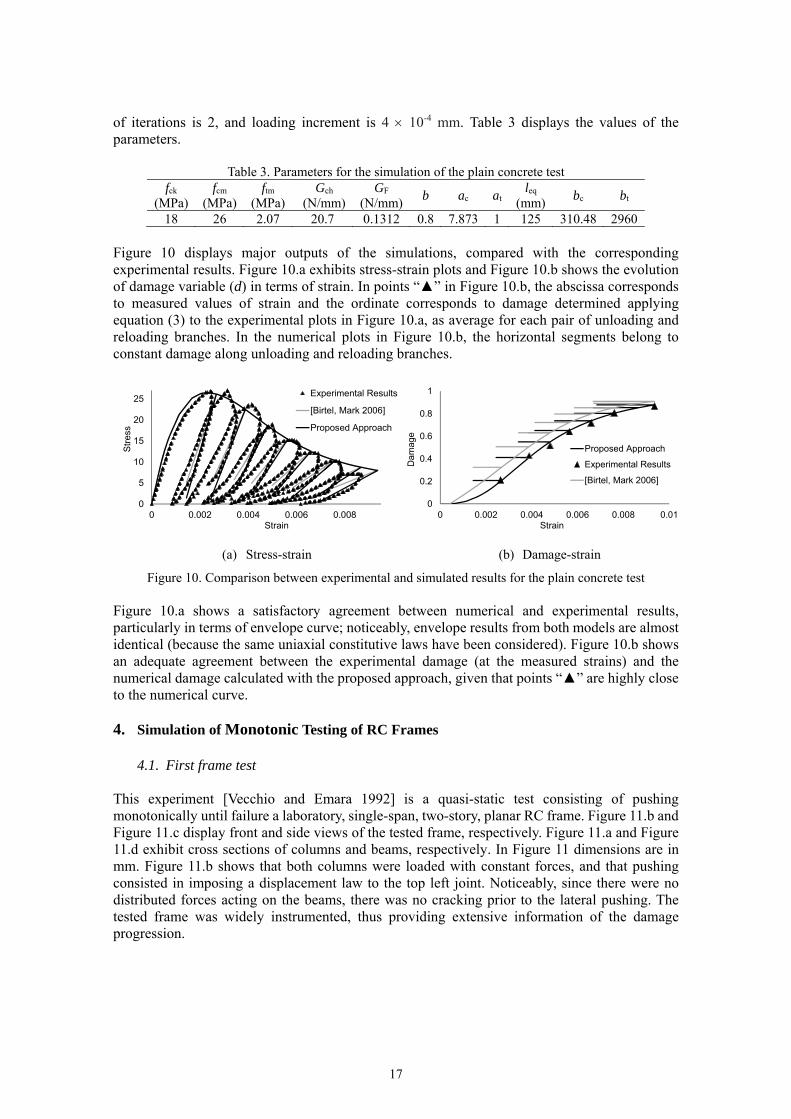
of iterations is 2, and loading increment is 4 10-4 mm. Table 3 displays the values of the parameters.

Table 3. Parameters for the simulation of the plain concrete test fck

(MPa) fcm

(MPa) ftm

(MPa) Gch

(N/mm) GF

(N/mm) b ac at

leq (mm)

bc bt

18 26 2.07 20.7 0.1312 0.8 7.873 1 125 310.48 2960 Figure 10 displays major outputs of the simulations, compared with the corresponding experimental results. Figure 10.a exhibits stress-strain plots and Figure 10.b shows the evolution of damage variable (d) in terms of strain. In points “▲” in Figure 10.b, the abscissa corresponds to measured values of strain and the ordinate corresponds to damage determined applying equation (3) to the experimental plots in Figure 10.a, as average for each pair of unloading and reloading branches. In the numerical plots in Figure 10.b, the horizontal segments belong to constant damage along unloading and reloading branches.

(a) Stress-strain (b) Damage-strain

Figure 10. Comparison between experimental and simulated results for the plain concrete test Figure 10.a shows a satisfactory agreement between numerical and experimental results, particularly in terms of envelope curve; noticeably, envelope results from both models are almost identical (because the same uniaxial constitutive laws have been considered). Figure 10.b shows an adequate agreement between the experimental damage (at the measured strains) and the numerical damage calculated with the proposed approach, given that points “▲” are highly close to the numerical curve. 4. Simulation of Monotonic Testing of RC Frames

4.1. First frame test

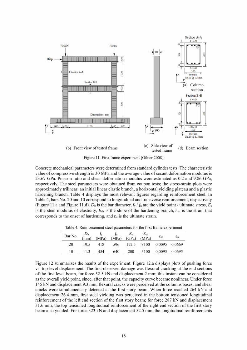
This experiment [Vecchio and Emara 1992] is a quasi-static test consisting of pushing monotonically until failure a laboratory, single-span, two-story, planar RC frame. Figure 11.b and Figure 11.c display front and side views of the tested frame, respectively. Figure 11.a and Figure 11.d exhibit cross sections of columns and beams, respectively. In Figure 11 dimensions are in mm. Figure 11.b shows that both columns were loaded with constant forces, and that pushing consisted in imposing a displacement law to the top left joint. Noticeably, since there were no distributed forces acting on the beams, there was no cracking prior to the lateral pushing. The tested frame was widely instrumented, thus providing extensive information of the damage progression.

0

5

10

15

20

25

0 0.002 0.004 0.006 0.008

Str

ess

Strain

Experimental Results

[Birtel, Mark 2006]

Proposed Approach

0

0.2

0.4

0.6

0.8

1

0 0.002 0.004 0.006 0.008 0.01

Da

mag

e

Strain

Proposed Approach

Experimental Results

[Birtel, Mark 2006]

18

(a) Column

section

(b) Front view of tested frame (c) Side view of

tested frame (d) Beam section

Figure 11. First frame experiment [Güner 2008] Concrete mechanical parameters were determined from standard cylinder tests. The characteristic value of compressive strength is 30 MPa and the average value of secant deformation modulus is 23.67 GPa. Poisson ratio and shear deformation modulus were estimated as 0.2 and 9.86 GPa, respectively. The steel parameters were obtained from coupon tests; the stress-strain plots were approximately trilinear: an initial linear elastic branch, a horizontal yielding plateau and a plastic hardening branch. Table 4 displays the most relevant figures regarding reinforcement steel. In Table 4, bars No. 20 and 10 correspond to longitudinal and transverse reinforcement, respectively (Figure 11.a and Figure 11.d). Db is the bar diameter, fy / fu are the yield point / ultimate stress, Es is the steel modulus of elasticity, Esh is the slope of the hardening branch, sh is the strain that corresponds to the onset of hardening, and u is the ultimate strain.

Table 4. Reinforcement steel parameters for the first frame experiment

Bar No. Db

(mm) fy

(MPa) fu

(MPa) Es

(GPa) Esh

(MPa) sh u

20 19.5 418 596 192.5 3100 0.0095 0.0669

10 11.3 454 640 200 3100 0.0095 0.0695

Figure 12 summarizes the results of the experiment. Figure 12.a displays plots of pushing force vs. top level displacement. The first observed damage was flexural cracking at the end sections of the first level beam, for force 52.5 kN and displacement 2 mm; this instant can be considered as the overall yield point, since, after that point, the capacity curve became nonlinear. Under force 145 kN and displacement 9.3 mm, flexural cracks were perceived at the columns bases, and shear cracks were simultaneously detected at the first story beam. When force reached 264 kN and displacement 26.4 mm, first steel yielding was perceived in the bottom tensioned longitudinal reinforcement of the left end section of the first story beam; for force 287 kN and displacement 31.6 mm, the top tensioned longitudinal reinforcement of the right end section of the first story beam also yielded. For force 323 kN and displacement 52.5 mm, the longitudinal reinforcements

x y

300

800 z y

x z

z y

19

of the column bases yielded as well, and hinges at the ends of the first story beam failed; this failure involved yielding of longitudinal reinforcement, and crushing of compressed concrete. Then, for force 329 kN and displacement 74.7 mm, similar failure was apparent at the column bases. Almost simultaneously, same failure affected at ends of second story beam. Afterwards, lateral stiffness was almost non-existent; therefore, collapse mechanism consisted in formation of six hinges. The experiment was terminated, for pushing force 332 kN and lateral displacement 150 mm, due to stroke limitations of the actuator, see Figure 12.a. Figure 12.b and Figure 12.c display images of the damaged bottom section of the right column, and the top left connection, respectively.

(a) Force-displacement plot (b) Right column base

(c) Top left connection

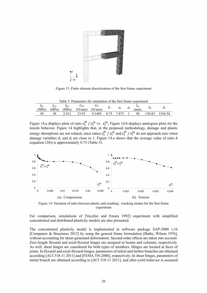
Figure 12. Results of first frame experiment [Vecchio and Emara 1992] The main objective of this experiment was to investigate the influence of shear-related effects in the overall structural behavior; the results showed that approximately 20% of the nonlinear lateral displacement was due to shear effects. Noticeably, at failure, around 12% of the overturning moment was due to P- effects. Supplementary information regarding this experiment is available in [Emara 1990]. This test had been previously simulated by some of the authors of this work [Barbat et al. 1997; Faleiro et al. 2005; Faleiro et al. 2008], and by other researchers [Güner 2008]. Barbat et al. used a viscous damage model, which was implemented in a fiber model with Timoshenko frame elements. Faleiro et al. implemented a damage plasticity formulation in a finite element model with planar 2D elements. Güner employed commercial software packages and an ad-hoc fiber model developed at University of Toronto. The [Vecchio and Emara 1992] test is simulated implementing the proposed methodology in Abaqus code [Abaqus 2013] by using the particular algorithm described in subsection 3.3. The maximum number of iterations is 10, and loading increment ranges between 10-11 mm and 0.01 mm. Table 5 displays the selected values of parameters. Figure 13 displays the finite element mesh; the left part depicts steel discretization with 2-node truss elements (T3D2) and the right part describes concrete discretization with 3D 8-node hexahedron solid elements (C3D8R).

20

Figure 13. Finite element discretization of the first frame experiment

Table 5. Parameters for simulation of the first frame experiment fck

(MPa) fcm

(MPa) ftm

(MPa) Gch

(N/mm) GF

(N/mm) b ac at

leq (mm)

bc bt

30 38 2.912 23.93 0.1405 0.75 7.873 1 50 156.83 1554.54

Figure 14.a displays plots of ratio ε /ε vs. ε ; Figure 14.b displays analogous plots for the tensile behavior. Figure 14 highlights that, in the proposed methodology, damage and plastic

energy absorptions are not related, since ratios ε /ε and ε /ε do not approach zero when damage variables dc and dt are close to 1. Figure 14.a shows that the average value of ratio b (equation (28)) is approximately 0.75 (Table 5).

(a) Compression (b) Tension

Figure 14. Variation of ratio between plastic and crushing / cracking strains for the first frame experiment

For comparison, simulations of [Vecchio and Emara 1992] experiment with simplified concentrated and distributed plasticity models are also presented. The concentrated plasticity model is implemented in software package SAP-2000 v.16 [Computers & Structures 2012] by using the general frame formulation [Bathe, Wilson 1976], without accounting for shear-generated deformation. Second-order effects are taken into account. Zero-length flexural and axial-flexural hinges are assigned to beams and columns, respectively. As well, shear hinges are considered for both types of members. Hinges are located at faces of joints. In flexural and axial-flexural hinges, parameters of initial and further branches are obtained according [ACI 318-11 2011] and [FEMA 356 2000], respectively. In shear hinges, parameters of initial branch are obtained according to [ACI 318-11 2011], and after-yield behavior is assumed

0

0.2

0.4

0.6

0.8

1

0 0.005 0.01 0.015 0.02 0.025

/ 

0

0.2

0.4

0.6

0.8

1

0 0.001 0.002 0.003 0.004

/ 

z x

y

21

to be totally brittle. Neither shear-flexural interaction nor shear-axial-flexural interaction is considered. The distributed plasticity models are implemented in package SeismoStruct V6.5 [Seismosoft 2013]. Two types of models are utilized to simulate both frame experiments. First type adopts the classical displacement-based finite element formulation [Hellesland, Scordelis 1981; Marí, Scordelis 1984] and second type is based on the more recent force-based formulation [Spacone et al. 1996; Neuenhofer, Filippou 1997]. Throughout this paper, these models are termed as DB and FB, respectively. FB approach does not impose any displacement field, and equilibrium is strictly and continuously satisfied. In the DB models, each member is discretized with four 2-node finite elements. In the FB models, a single element with five integration points represents each member. For both FB and DB models, sections are discretized into 250 fibers. Second-order effects are accounted for. As in the concentrated plasticity model, the interaction between shear and flexure is not taken into consideration. Figure 15 displays experimental results (Figure 12.a) plotted together with numerical results obtained with the proposed methodology and the abovementioned simplified models. Descriptions of observed damage states are also displayed.

Figure 15. Experimental and simulated capacity curves for the first frame experiment Plots from Figure 15 show the superior ability of the proposed methodology to reproduce the experimental results along the whole displacement range. It captures the initial stiffness, the onset of overall yielding, the sequence of damage progression and the final state. Noticeably, “overall yielding” does not refer to steel yielding but to inception of overall nonlinear behavior, due to cracking of tensioned concrete. Regarding the lumped plasticity model, accuracy can be considered satisfactory, given the important simplifications involved in that model. Figure 15 shows that the concentrated model describes satisfactorily the initial slope, but fails to predict the cracking and, therefore, the onset of overall yielding. The yielding branch is almost horizontal because of second order effects. The maximum capacity in terms of force is underestimated because of the conservative assumptions in the predefined plastic hinges. The final failure is earlier because the actual ductility of members is also underestimated by the assumed moment-rotation laws. Regarding the distributed plasticity models, Figure 15 shows that they perform better, particularly FB. DB model exhibits less accuracy, because the mesh is too coarse. However,

0

50

100

150

200

250

300

350

0 0.02 0.04 0.06 0.08 0.1 0.12 0.14 0.16 0.18

Fo

rce

(KN

)

Displacement (m)

Experimental Results

Concentrated Plasticity Model

Distributed Plasticity Model (FB)

Distributed Plasticity Model (DB)

Proposed Approach

1st story beam steel yielding264 kN, 26.4 mm

1st story beam steel yielding

287 kN, 31.6 mm

column bases steel yielding 1st story beam hinging

323 kN, 52.5 mm column bases hinging 2nd story beam hinging

329 kN, 74.7 mm

1st story beam cracking52.5 kN, 2 mm

column base cracking1st story beam cracking

145 kN, 9.3 mm

22

these models cannot capture adequately the gradual progression of the global softening after the initial overall yielding, due to lack of consideration of the concrete tensile strength. Noticeably, the negative slope of the final branches is due to second-order effects. To further highlight the capacity of the proposed methodology to capture damage progression, Figure 16 through Figure 18 display the damage predicted for some of the previously described stages. Figure 16 displays the distribution of the tensile damage variable for force 52.5 kN and top level displacement 2 mm; it corresponds to the first cracking at end sections of 1st story beam. Figure 16.a and Figure 16.b refer to the first story right beam-column connection and to the overall frame, respectively. Figure 16.a shows that cracking (indicated with lighter gray) actually occurred in the top part of beam, since the tensile damage variable reaches values close to one. Figure 16.b shows that the overall distribution of cracking fits the expected pattern according to structural analysis principles, with onset of cracking in the bottom part of the first story right beam-column connection.

(a) Distribution of dt at the first story right

beam-column connection (b) Distribution of dt at the frame

Figure 16. Tensile damage variable for force 52.5 kN and displacement 2 mm for the first frame experiment

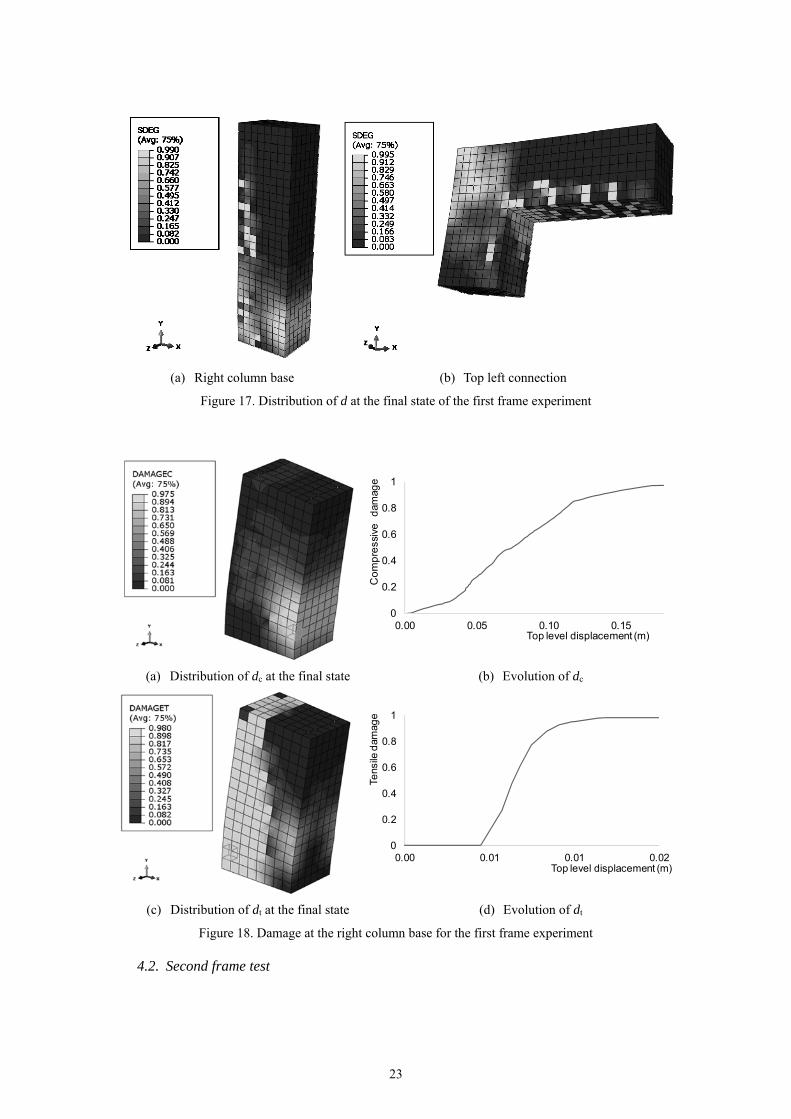
Figure 17 and Figure 18 refer to the final state. Figure 17.a and Figure 17.b display distributions of the scalar damage variable (d) for the right column base and the top left beam-column connection, respectively. Figure 18 refers to the right column base, describing both the final state and the evolution from the undamaged state. Figure 18.a and Figure 18.c represent the distribution of the compressive and tensile damage variables, respectively; Figure 18.b and Figure 18.d display, for selected finite elements, plots of such variables vs. top level displacement, respectively. In all the images, higher damage corresponds to lighter grey. Figure 17 and Figure 18 show that the observed phenomena are adequately reproduced by the proposed methodology, since the obtained damage distributions fit the expected results. Comparison between Figure 17.a and the observed damage in Figure 12.b shows a satisfactory fit, since cracking and crushing are detected by the obtained higher values of d. Comparison between Figure 17.b and the observed damage in Figure 12.c shows also a satisfactory match. Figure 18.a and Figure 18.c show that there is hinging, since both damage variables attain values close to 1; this circumstance is observed in Figure 12.b. Figure 18.b and Figure 18.d show that cracking occurs for smaller displacement (approximately 10 mm) than crushing (more than 150 mm).

23

(a) Right column base (b) Top left connection

Figure 17. Distribution of d at the final state of the first frame experiment

(a) Distribution of dc at the final state (b) Evolution of dc

(c) Distribution of dt at the final state (d) Evolution of dt

Figure 18. Damage at the right column base for the first frame experiment

4.2. Second frame test

0

0.2

0.4

0.6

0.8

1

0.00 0.05 0.10 0.15

Co

mp

ress

ive

d

amag

e

Top level displacement (m)

0

0.2

0.4

0.6

0.8

1

0.00 0.01 0.01 0.02

Tens

ile d

amag

e

Top level displacement (m)

24

This experiment [Pires 1990] is a quasi-static test consisting of imposing a displacement law to a laboratory single-span, single-story 2-D RC frame. Figure 19.b describes the tested frame, and Figure 19.a and Figure 19.c display beam and columns sections, respectively. Figure 19.b shows that both columns were loaded with constant forces and that displacement was imposed to the top left joint. Noticeably, as in the first frame test, given the absence of distributed loads on beams, there was no initial cracking.

(a) Beam section

(b) Tested frame (c) Column section

Figure 19. Second frame experiment [Braz-César et al. 2008a,b] Mechanical parameters of materials are based on nominal values. The characteristic value of the concrete compressive strength is 20 MPa (C20/25, [EN 1992 2004]), and the steel yield point is 400 MPa for the longitudinal reinforcement and 500 MPa for the stirrups [EN 10080 2006]. As described in Figure 19.c, in the critical end segments (“confinement sections”), closer stirrup spacing was used; the lengths of these segments are 40 cm in beam and 30 cm in columns. This frame had been previously simulated by [Braz-César et al. 2008a,b] by using concentrated and distributed plasticity models. Analogously to [Vecchio and Emara 1992] experiment, this test is simulated implementing the algorithm in Abaqus code [Abaqus 2013]. The maximum number of iterations is 10, and loading increment ranges between 0.0001 mm and 0.01 mm. Table 6 displays the selected values of the parameters.

Table 6. Parameters for simulation of the second frame experiment fck

(MPa) fcm

(MPa) ftm

(MPa) Gch

(N/mm) GF

(N/mm) b ac at

leq (mm)

bc bt

20 28 2.222 21.12 0.133 0.9 7.873 1 25 65.48 626.67 The [Pires 1990] experiment is simulated with the proposed methodology. For comparison, simulations with simplified concentrated and distributed plasticity models are also included. Similarly to Figure 15, Figure 20 displays experimental results together with numerical results from the proposed approach and the said simplified models. FB and DB refer to force-based and displacement-based, respectively.

x y

z y

x z

25

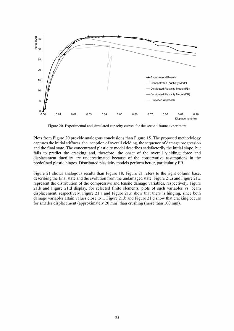
Figure 20. Experimental and simulated capacity curves for the second frame experiment

Plots from Figure 20 provide analogous conclusions than Figure 15. The proposed methodology captures the initial stiffness, the inception of overall yielding, the sequence of damage progression and the final state. The concentrated plasticity model describes satisfactorily the initial slope, but fails to predict the cracking and, therefore, the onset of the overall yielding; force and displacement ductility are underestimated because of the conservative assumptions in the predefined plastic hinges. Distributed plasticity models perform better, particularly FB. Figure 21 shows analogous results than Figure 18. Figure 21 refers to the right column base, describing the final state and the evolution from the undamaged state. Figure 21.a and Figure 21.c represent the distribution of the compressive and tensile damage variables, respectively. Figure 21.b and Figure 21.d display, for selected finite elements, plots of such variables vs. beam displacement, respectively. Figure 21.a and Figure 21.c show that there is hinging, since both damage variables attain values close to 1. Figure 21.b and Figure 21.d show that cracking occurs for smaller displacement (approximately 20 mm) than crushing (more than 100 mm).

0

5

10

15

20

25

30

35

0.00 0.01 0.02 0.03 0.04 0.05 0.06 0.07 0.08 0.09 0.10

For

ce (

KN

)

Displacement (m)

Experimental Results

Concentrated Plasticity Model

Distributed Plasticity Model (FB)

Distributed Plasticity Model (DB)

Proposed Approach

26

(a) Distribution of dc at the final state

(b) Evolution of dc

(c) Distribution of dt at the final state (d) Evolution of dt

Figure 21. Damage at the right column base for the second frame experiment 5. Conclusions

This paper presents a new methodology to calculate damage variables for Concrete Plastic Damage Models suitable for describing the monotonic behavior of reinforced concrete structures. The proposed approach is mesh-insensitive, is based on a sound continuum mechanics formulation, and does not require calibration with experimental results. Implementation is straightforward; a particular algorithm is presented. Mesh-insensitivity is validated in a simple tension example. Accuracy and reliability are verified by simulating a cyclic experiment on plain concrete specimens and two tests consisting in pushing monotonically until failure two laboratory 2-D RC frames. Results on these frames are compared with simplified models commonly employed in earthquake engineering. Tension example. This example confirms the mesh-insensitiveness of the proposed methodology. As well, numerical results match analytical ones, thus ratifying their accuracy. Cyclic experiment. The simulation of the cyclic experiment on plain concrete corroborates the capacity of the proposed approach to reproduce damage evolution and stress-strain behavior, both in terms of envelope curve and stiffness degradation at each unloading / reloading cycle. Agreement between experimental and numerical damage at measured strain levels is satisfactory. Frame experiments. The simulation of the frame tests proves the ability of the proposed methodology to reproduce accurately the experimental force-displacement results along the whole displacement range. Captures initial stiffness, onset of the overall yielding, sequence of the

0

0.2

0.4

0.6

0.8

1

0.00 0.02 0.04 0.06 0.08 0.10

Co

mp

ress

ive

dam

age

Lateral displacement (m)

0

0.2

0.4

0.6

0.8

1

0.00 0.01 0.02 0.03 0.04 0.05

Tens

ile d

amag

e

Lateral displacement (m)

27

damage progression, collapse mechanism, and final state. All failure and degradation modes are adequately simulated: tensioned concrete cracking, compressed concrete crushing, and reinforcement steel yielding. The aforementioned simplified models provide less accuracy, being not able to reproduce all the involved phenomena. Research for extending the proposed methodology to cyclic comportment of RC structures is currently in progress. The final objective is to derive models that are appropriate for simulating complex behavior of RC structures under strong ground motions. Acknowledgements

This work has received financial support from Spanish Government under projects BIA2014-60093-R, MAT2014-60647-R and CGL2015-6591 and from European Commission under projects ERC-2012-AdG-320815 and PIRSES-GA-2013-612607. These supports are gratefully acknowledged. References

[1] Al-Rub A, Voyiadjis GZ (2009). Gradient-enhanced coupled plasticity an isotropic damage model for concrete fracture: computational aspects and applications. International Journal of Damage Mechanics 18, 115–154.

[2] Al-Rub A, Kim S-M (2010). Computational applications of a coupled plasticity-damage constitutive model for simulating plain concrete fracture, Engineering Fracture Mechanics. 77 (2010) 1577–1603. doi:10.1016/j.engfracmech.2010.04.007.

[3] Abaqus analysis user’s manual version 6.11.3. (2013). Pawtucket (RI): Hibbitt, Karlsson & Sorensen. [4] ACI 318-11 (2011). Building Code Requirements for Structural Concrete. American Concrete

Institute. [5] Addessi D, Marfia S, Sacco E (2002). A plastic nonlocal damage model. Computer Methods in

Applied Mechanics and Engineering 191, 1291–1310. [6] Aslani F, Jowkarmeimandi R (2012). Stress-strain model for concrete under cyclic loading. Magazine

of Concrete Research. 64 (8):673-685. [7] Barbat AH, Oller S, Oñate E, Hanganu A (1997). Viscous damage model for Timoshenko beam

structures, International Journal of Solids and Structures. 34(30) 3953-3976. [8] Bathe KJ, Wilson EL (1976). Numerical Methods in Finite Element Analysis, Prentice-Hall. [9] Bazant ZP, Oh BH (1983). Crack Band Theory for Fracture of Concrete, Mat. Construction (RILEM)

16:155-177. [10] Bazant ZP, Belytschko T, Chang TP (1984). Continuum theory for strain-softening, J. Eng. Mech.,

110, 1666-1692. [11] Bazant ZP, Pijaudier-Cabot G (1988). Nonlocal continuum damage, localization instability and

convergence. Journal of Applied Mechanics 55, 287-293 [12] Belytschko T, Fish J, Engelmann BE. (1988). A finite element with embedded localization zones.

Computer Methods in Applied Mechanics and Engineering 70:59-89. [13] Birtel V, Mark P (2006). Parametrised Finite Element Modelling of RC Beam Shear Failure. Abaqus

Users Conference 95-108. [14] Braz-César MT, Oliveira D, Barros RC (2008a). Comparison of cyclic response of reinforced concrete

infilled frames with experimental results, 14th World Conference on Earthquake Engineering (14WCEE), Beijing, China.

[15] Braz-César MT, Oliveira D, Barros RC (2008b). Numerical validation of the experimental cyclic response of reinforced concrete frames. In “Trends in Computational Structures Technology” Topping BHV, Papadrakakis M Eds., Saxe-Coburg.

[16] Burlion N, Gatuingt F, Pijaudier-Cabot G, Daudeville L. (2000). Compaction and tensile damage in concrete: constitutive modelling and application to dynamics, Comput. Methods Appl. Mech. Engrg. 183:291-308

[17] Carol I, Rizzi E., Willam KJ. (2001). On the formulation of anisotropic elastics degradation. II.

28

Generalized pseudo-Rankine model for tensile damage. International Journal of Solids and Structures 38, 519–546.

[18] Castro JC, López Almansa F, Oller S (2014). Modelización numérica del comportamiento estructural cíclico de barras esbeltas de acero con pandeo restringido, RIMNI. 30(4) 229-237. DOI: 10.1016/j.rimni.2013.07.008.

[19] CEB-FIP (2010). Model Code 2010. Thomas Telford, London. [20] Challamel N, Lanos C, Casandjian C (2005). Strain-based anisotropic damage modelling and

unilateral effects. Int. J. Mech. Sc. 47, 459–473. [21] Chen AC, Chen WF. (1975). Constitutive relations for concrete. Journal of Engineering Mechanics

Division, ASCE 101, 465–481. [22] Cicekli U, Voyiadjis G, Al-Rub A (2007). A plasticity and anisotropic damage model for plain

concrete. International Journal of Plasticity, 23, 1874-1900. [23] Computers & Structures Inc. (2012). CSI Analysis Reference Manual for SAP2000®, ETABS®, and

SAFE™, available from www.comp-engineering.com. [24] Emara MB (1990). Shear Deformations in Reinforced Concrete Frames, M.A.Sc. Thesis, Department

of Civil Engineering, University of Toronto. [25] EN 10080 (2006). Steel for the reinforcement of concrete, weldable, ribbed reinforcing steel.

European Committee for Standardization. [26] EN 1992 (2004). Eurocode 2: Design of concrete structures. European Committee for Standardization. [27] Faleiro J, Barbat A, Oller S (2005). Plastic damage model for nonlinear reinforced concrete frames

analysis, VIII International Conference on Computational Plasticity (COMPLAS VIII), CIMNE. [28] Faleiro J, Oller S, Barbat A (2008). Plastic-damage analysis of reinforced concrete frames,

Engineering Computations, 27(1):57-83. [29] Faria R, Oliver J, Cervera M. (1998). A strain-based plastic viscous-damage model for massive

concrete structures, Int. J. Solids Structures 35(14), 1533-1558 [30] Fichant S, La Borderie C, Cabot G P (1999). Isotropic and anisotropic descriptions of damage in

concrete structures, Mechanics of Cohesive‐frictional Materials 4 (4), 339-359 [31] FEMA 356 (2000). Prestandard and commentary for the seismic rehabilitation of buildings, Federal

Emergency management Agency. [32] Grassl P, Jirásek M (2006a). Damage-plastic model for concrete failure. International Journal of

Solids and Structures, 43(22-23):7166-7196. (doi:10.1016/j.ijsolstr.2006.06.032). [33] Grassl, P, Jirásek M (2006b). Plastic model with non-local damage applied to concrete. International

Journal for Numerical and Analytical Methods in Geomechanics 30, 71–90. [34] Güner S (2008). Performance assessment of shear-critical reinforced concrete plane frames, PhD.

Thesis, University of Toronto. [35] Govindjee S, Kay G, Simo JC (1995). Anisotropic modeling and numerical simulation of brittle

damage in concrete. Int. J. Num. Methods Eng., 38(21), 3611-363 [36] Häussler-Combe U, Hartig J (2008). Formulation and numerical implementation of a constitutive law

for concrete with strain-based damage and plasticity. International Journal of Non-Linear Mechanics 43:399–415. doi:10.1016/j.ijnonlinmec.2008.01.005.

[37] Halm D, Dragon A (1998). An anisotropic model of damage and frictional sliding for brittle materials. Eur. J. Mech. and Solids 17, 439– 460.

[38] Hansen E, Willam K, Carol I (2001). A two-surface anisotropic damage/plasticity model for plain concrete, Fracture Mechanics of Concrete Structures. Balkema, Lisse, pp. 549–556

[39] Hellesland J, Scordelis A (1981). Analysis of RC bridge columns under imposed deformations, IABSE Colloquium, Delft 545-559.

[40] Hordijk, DA (1992). Tensile and tensile fatigue behavior of concrete; experiments, modeling and analyses, Heron 37(1):3-79.

[41] Jansen DC, Shah SP (1997). Effect of length on compressive strain softening of concrete. J.Eng.Mech. ASCE, 123 (1), 25-35

[42] Jason L, Huerta A, Pijaudier-Cabot G, Ghavamian S (2006). An elastic plastic damage formulation for concrete: application to elementary tests and comparison with an isotropic damage model. Computer Methods in Applied Mechanics and Engineering 195, 7077–7092.

[43] Jirásek, Zimmermann (2001). Embedded crack model: I. Basic formulation. Int. J. Numer. Meth.

29

Engng 50:1269–1290. [44] Ju JW (1989). On energy-based coupled elasto-plastic damage theories: constitutive modeling and

computational aspects. Int. J Sol. Struct. 25:803–833. [45] Krätzig WB, Pölling R (2004). An elasto-plastic damage model for reinforced concrete with minimum

number of material parameters, Computer and Structures 82(15-16): 1201–1215. [46] Kotsovos MD (1983). Effect of testing techniques on the post-ultimate behaviour of concrete in

compression. Mater. Struct. (RILEM), 16(1):3–12. [47] Lee J, Fenves GL (1998). Plastic-Damage Model for Cyclic Loading of Concrete Structures,

Engineering Mechanics 124(8):892–900. [48] Lemaitre J. (1992). A course on damage mechanics, Springer Verlag. [49] Lykidis GC, Spiliopoulos KV (2008). 3D Solid Finite-Element Analysis of Cyclically Loaded RC

Structures Allowing Embedded Reinforcement Slippage, Journal of Structural Engineering, 134(4): 629–638.

[50] Lin FB, Bazant ZP, Chern JC, Marchertas AH. (1987). Concrete model with normality and sequential identification. Computers and Structures 26:1011–1025.

[51] López-Almansa F, Castro JC, Oller S (2012). A numerical model of the structural behavior of buckling-restrained braces, Engineering Structures, 41(1):108–117.

[52] López-Almansa F, Alfarah B, Oller S (2014). Numerical simulation of RC frame testing with Damage Plasticity Model, 15th European Conference on Earthquake Engineering (15ECEE), Istanbul, Turkey.

[53] Lubliner J, Oliver J, Oller S, Oñate E (1989). A plastic-damage model for concrete, Solids and Structures, 25(3):299–326.

[54] Luccioni B, Oller S, Danesi R. (1996). Coupled plastic-damaged model, Comput. Methods Appl. Mech. Engrg 129:81-89.

[55] Marí A, Scordelis A (1984). Nonlinear geometric material and time dependent analysis of three dimensional reinforced and prestressed concrete frames, Report 82-12, University of California, Berkeley.

[56] Markeset G, Hillerborg A (1995), Softening of concrete in compression-Localization and size effects. Cement and Concrete Research, 25(44) 702-708.

[57] Mazars J. (1984). Application de la mécanique de l'endommagement au comportement non linéaire et à la rupture du béton de structure. Doctoral thesis, University of Paris.

[58] Mazars J, Pijaudier-Cabot G. (1989). Continuum damage theory-application to concrete. Journal of Engineering Mechanics ASCE, 115(2):345–365.

[59] Meschke G, Lackner R, Mang H (1998). An anisotropic elastoplastic-damage model for plain concrete. Int. J Num. Meth. Eng., 42, 703-727.

[60] Mosalam KM, GH Paulino. (1997). Evolutionary Characteristic Length Method for Smeared Cracking Finite Element models, Finite Element in Analysis and Design, 27(1):99-108.

[61] Neuenhofer A, Filippou FC (1997). Evaluation of nonlinear frame finite-element models, Structural Engineering, 123(7): 958-966.

[62] Nguyen GD, HoulsbyG.T. (2004). A thermodynamic approach to constitutive modelling of concrete, Proceedings of the 12th conference, Association for Computational Mechanics in Engineering (ACME-UK), Cardiff UK.

[63] Nguyen GD, Korsunsky A. (2008). Development of an approach to constitutive modelling of concrete: damage coupled with plasticity. International Journal of Solids and Structures, 45(20), 5483-5501.

[64] Oliver J. (1989). A consistent characteristic length for smeared cracking models. Int J Numer Methods Engng; 28:461–74.

[65] Oller S (1988). A continuous damage model for frictional materials (in Spanish), Doctoral Dissertation, Technical University of Catalonia.

[66] Oller S (2014). Nonlinear Dynamics, International Center for Numerical Methods in Engineering, Technical University of Catalonia.

[67] Ortiz M (1985). A constitutive theory for the inelastic behavior of concrete. Mech. Mater. 4, 67–93. [68] Pires F (1990). Influência das paredes de alvenaria no comportamento de estruturas reticuladas de

betão armado sujeitas a acções horizontais, PhD Thesis, LNEC, Lisbon, Portugal (in Portuguese). [69] Peerlings RHJ, R. de Borst, Brekelmans WAM, Geers MGD (1998). Gradient-enhanced damage

30

modeling of concrete fracture. Mech. Cohesive-Frictional Mat., 3, 323-343. [70] Salari MR, Saeb S, Willam KJ, Patchet SJ, and Carrasco RC. (2004). A coupled elastoplastic damage

model for geomaterials, Comput. Methods Appl. Mech. Engrg 193(27-29), 2625-2643. [71] Seismosoft (2013). SeismoStruct v6.5 – A computer program for static and dynamic nonlinear

analysis of framed structures, available from http://www.seismosoft.com. [72] Simo JC, Oliver J. (1994). A new approach to the analysis and simulation of strain softening in solids.

In Fracture and Damage in Quasibrittle Structures, E&FN:25-39. [73] Simo JC, Ju JW (1987). Strain- and stress-based continuum damage models—I. Formulation. Int. J.

Solids Struct. 23, 821–840. [74] Sinha BP, Gerstle KH, Tulin LG (1964). Stress-strain relations for concrete under cyclic loading, ACI

Structural Journal 62(2):195-210. [75] Spacone E, Ciampi V, Filippou FC (1996). Mixed formulation of nonlinear beam finite element,

Computers & Structures, 58(1):71-83. [76] Van Mier, JGM (1984). Strain-softening of concrete under multiaxial loading conditions PhD Thesis,

Technical University of Eindhoven. [77] Van Mier JGM, Vonk RA (1991). Fracture of concrete under multiaxial stress: Recent developments.

Mater. Struct. (RILEM), 24(1): 61–65. [78] Van Mier JGM (2013). Concrete Fracture A Multiscale Approach, Taylor & Francis. [79] Vecchio F, Emara MB (1992). Shear Deformations in reinforced Concrete Frames, ACI Structural

Journal, 89(1):46-56. [80] Vermeer PA, de Borst R (1984). Non-associated plasticity for soils, concrete and rock, Heron 29(3):3–

64. [81] Vonk RA (1993). A micromechanical investigation of softening of concrete loaded in compression,

Heron 38(3):3-94. [82] Voyiadjis GZ, Ziad N. Taqieddin, Kattan PI. (2008). Anisotropic damage–plasticity model for

concrete. International Journal of Plasticity 24:1946–1965.

[83] Yu T, Teng JG, Won YL, Dong SL (2010). Finite element modeling of confined concrete-II: Plastic-damage model. Journal of Engineering Structures 32:680–691. doi:10.1016/j.engstruct.2009.11.013.

List of symbols

Roman letters. Lower case ac / at / bc / bt: dimensionless coefficients in equations (15) and (16)

b: ε /ε ratio (equation (28)) c / c1 / c2: cohesion / coefficients in equation (29) d / dc / dt: damage variable / compression damage variable / tension damage variable f / fb0 / fc0 / fcm / ftm / fc0 / ft0 / fck: stress strength / biaxial compressive yield strength / uniaxial compressive

yield strength / concrete compressive stress strength / concrete tensile stress strength / limit stress of linear compressive branch / limit stress of linear tensile branch / characteristic value of concrete compressive strength

fy / fu: steel yield point / ultimate stress gc / gt: compressive / tensile energies per unit volume dissipated by damage along entire deterioration

process / : weighting factors accounting for stiffness recovery

leq: mesh size (finite element characteristic length) p: hydrostatic pressure stress q: Von Mises-equivalent effective stress r*: stress state; for uniaxial stress r*(11) = 1 for tension and r*(11) = 0 for compression sc / st: coefficients accounting for stress state and stiffness recovery effects w / wc: crack opening / crack opening at fracture Roman letters. Upper case Db: reinforcement bar diameter

31

E / E0 / Eci: modulus of deformation / undamaged modulus of deformation / tangent modulus of deformation of concrete for zero stress

Es / Esh: steel modulus of elasticity / slope of hardening branch F: loading function G / Gch / GF: flow potential / crushing energy per unit area / fracture energy per unit area H: Mohr-Coulomb yield surface function I1: first invariant of stress tensor J2 / J3: second / third invariants of deviatoric stress tensor Kc: ratio of second stress invariants on tensile and compressive meridians Greek letters / c / t / el / pl / cm / tm: strain / compression strain / tensile strain / elastic strain / plastic strain / strain

at compressive strength / strain at tensile strength

ε / ε /ε /ε /ε /ε / ε /ε : strains at Figure 5; subindexes “c”, “t”, “0c” and “0t” and refer to compression, tension, undamaged compression and undamaged tension, respectively; superindexes “pl”, “el”, “ch” and “ck” and refer to plastic, elastic, crushing and cracking, respectively sh / u: steel strain that corresponds to onset of hardening / ultimate strain ϵ: eccentricity of the plastic potential surface ϕ: friction angle : Lode similarity angle : octahedral radius / 11 / σt0 / σc(1) / σc(2) / σc(3): stress / first principal uniaxial stress / uniaxial tensile stress at failure / concrete

compressive stress at first / second / third segment / : effective compressive / tensile cohesion stress

: distance from origin of stress space to stress plan ѱ: dilatancy angle