This chapter presents an axiomatic approach for reformulating radial ba-sis function (RBF) neural networks. With this approach the constructionof admissible RBF models is reduced to the selection of generator func-tions that satisfy certain properties. The selection of specific generatorfunctions is based on criteria which relate to their behavior when thetraining of reformulated RBF networks is performed by gradient descent.This chapter also presents batch and sequential learning algorithms de-veloped for reformulated RBF networks using gradient descent. Thesealgorithms are used to train reformulated RBF networks to recognizehandwritten digits from the NIST databases.
1 Introduction
A radial basis function(RBF) neural network is usually trained to mapa vectorxk 2 IRni into a vectoryk 2 IRno, where the pairs(xk;yk); 1 �k � M , form thetraining set. If this mapping is viewed as a functionin the input spaceIRni , learning can be seen as a function approxima-tion problem. From this point of view, learning is equivalent to findinga surface in a multidimensional space that provides the best fit for thetraining data. Generalization is therefore synonymous with interpolationbetween the data points along the constrained surface generated by thefitting procedure as the optimum approximation to this mapping.
Broomhead and Lowe [3] were the first to explore the use of radial basisfunctions in the design of neural networks and to show how RBF neu-ral networks model nonlinear relationships and implement interpolation.Micchelli [33] showed that RBF neural networks can produce an inter-polating surface which exactly passes through all the pairs of the trainingset. However, the exact fit is neither useful nor desirable in practice as itmay produce anomalous interpolation surfaces. Poggio and Girosi [38]viewed the training of RBF neural networks as an ill-posed problem,in the sense that the information in the training data is not sufficient touniquely reconstruct the mapping in regions where data are not available.From this point of view, learning is closely related to classical approxi-mation techniques such as generalized splines and regularization theory.Park and Sandberg [36], [37] proved that RBF neural networks with onelayer of radial basis functions are capable of universal approximation.Under certain mild conditions on radial basis functions, RBF networksare capable of approximating arbitrarily well any function. Similar proofsalso exist in the literature for feed-forward neural models with sigmoidalnonlinearities [7].
The performance of a RBF neural network depends on the number andpositions of the radial basis functions, their shapes, and the method usedfor learning the input-output mapping. The existing learning strategiesfor RBF neural networks can be classified as follows: 1) strategies se-lecting radial basis function centers randomly from the training data [3],2) strategies employing unsupervised procedures for selecting radial ba-sis function centers [5], [6], [25], [34], and 3) strategies employing su-
pervised procedures for selecting radial basis function centers [4], [13],[17], [20], [21], [38].
Broomhead and Lowe [3] suggested that, in the absence ofa prioriknowledge, the centers of the radial basis functions can either be dis-tributed uniformly within the region of the input space for which thereis data, or chosen to be a subset of training points by analogy withstrict interpolation. This approach is sensible only if the training data aredistributed in a representative manner for the problem under considera-tion, an assumption that is very rarely satisfied in practical applications.Moody and Darken [34] proposed a hybrid learning process for train-ing RBF neural networks with Gaussian radial basis functions, whichis widely used in practice. This learning procedure employs differentschemes for updating theoutput weights, i.e., the weights that connectthe radial basis functions with the output units, and the centers of theradial basis functions, i.e., the vectors in the input space that representthe prototypesof the input vectors included in the training set. Moodyand Darken used thec-means (ork-means) clustering algorithm [2] anda “P -nearest-neighbor” heuristic to determine the positions and widthsof the Gaussian radial basis functions, respectively. The output weightsare updated using a supervised least-mean-squares learning rule. Pog-gio and Girosi [38] proposed a fully supervised approach for trainingRBF neural networks with Gaussian radial basis functions, which up-dates the radial basis function centers together with the output weights.Poggio and Girosi used Green’s formulas to deduct an optimal solutionwith respect to the objective function and employed gradient descent toapproximate the regularized solution. They also proposed that Kohonen’sself-organizing feature map [29], [30] can be used for initializing the ra-dial basis function centers before gradient descent is used to adjust all ofthe free parameters of the network. Chenet al. [5], [6] proposed a learn-ing procedure for RBF neural networks based on theorthogonal leastsquares(OLS) method. The OLS method is used as a forward regres-sion procedure to select a suitable set of radial basis function centers. Infact, this approach selects radial basis function centers one by one untilan adequate RBF neural network has been constructed. Cha and Kas-sam [4] proposed a stochastic gradient training algorithm for RBF neuralnetworks with Gaussian radial basis functions. This algorithm uses gradi-ent descent to update all free parameters of RBF neural networks, which
include the radial basis function centers, the widths of the Gaussian ra-dial basis functions, and the output weights. Whitehead and Choate [42]proposed an evolutionary training algorithm for RBF neural networks.In this approach, the centers of radial basis functions are governed byspace-filling curves whose parameters evolve genetically. This encodingcauses each group of co-determined basis functions to evolve in order tofit a region of the input space. Royet al. [40] proposed a set of learn-ing principles that led to a training algorithm for a network that contains“truncated” radial basis functions and other types of hidden units. Thisalgorithm uses random clustering and linear programming to design andtrain the network with polynomial time complexity.
Despite the existence of a variety of learning schemes, RBF neural net-works are frequently trained in practice using variations of the learn-ing scheme proposed by Moody and Darken [34]. These hybrid learn-ing schemes determine separately the prototypes that represent the ra-dial basis function centers according to someunsupervisedclustering orvector quantization algorithm and update the output weights by asuper-visedprocedure to implement the desired input-output mapping. Theseapproaches were developed as a natural reaction to the long trainingtimes typically associated with the training of traditional feed-forwardneural networks using gradient descent [28]. In fact, these hybrid learn-ing schemes achieve fast training of RBF neural networks as a result ofthe strategy they employ for learning the desired input-output mapping.However, the same strategy prevents the training set from participating inthe formation of the radial basis function centers, with a negative impacton the performance of trained RBF neural networks [25]. This createda wrong impression about the actual capabilities of an otherwise pow-erful neural model. The training of RBF neural networks using gradientdescent offers a solution to the trade-off between performance and train-ing speed. Moreover, such training can make RBF neural networks seri-ous competitors to feed-forward neural networks with sigmoidal hiddenunits.
Learning schemes attempting to train RBF neural networks by fixing thelocations of the radial basis function centers are very slightly affected bythe specific form of the radial basis functions used. On the other hand,the convergence of gradient descent learning and the performance of the
trained RBF neural networks are both affected rather strongly by thechoice of radial basis functions. The search for admissible radial basisfunctions other than the Gaussian function motivated the developmentof an axiomatic approach for constructing reformulated RBF neural net-works suitable for gradient descent learning [13], [17], [20], [21].
2 Function Approximation Models andRBF Neural Networks
There are many similarities between RBF neural networks and functionapproximation models used to perform interpolation. Such function ap-proximation models attempt to determine a surface in a Euclidean spaceIRni that provides the best fit for the data(xk; yk), 1 � k � M , wherexk 2 X � IRni andyk 2 IR for all k = 1; 2; : : : M . Micchelli [33] con-sidered the solution of the interpolation problems(xk) = yk; 1 � k �M , by functionss : IRni ! IR of the form:
s(x) =MXk=1
wk g(kx� xkk2): (1)
This formulation treats interpolation as a function approximation prob-lem, with the functions(�) generated by the fitting procedure as the bestapproximation to this mapping. Given the form of the basis functiong(�),the function approximation problem described bys(xk) = yk; 1 � k �M , reduces to determining the weightswk; 1 � k �M , associated withthe model (1).
The model described by equation (1) is admissible for interpolation ifthe basis functiong(�) satisfies certain conditions. Micchelli [33] showedthat a functiong(�) can be used to solve this interpolation problem if theM�M matrixG = [gij] with entriesgij = g(kxi�xjk
2) is positive def-inite. The matrixG is positive definite if the functiong(�) is completelymonotonicon (0;1). A functiong(�) is called completely monotonic on(0;1) if it is continuous on(0;1) and its`th order derivativesg(`)(x)satisfy(�1)` g(`)(x) � 0; 8x 2 (0;1), for ` = 0; 1; 2; : : :.
RBF neural network models can be viewed as the natural extension ofthis formulation. Consider the function approximation model described
If the functiong(�) satisfies certain conditions, the model (2) can be usedto implement a desired mappingIRni ! IR specified by the trainingset (xk; yk); 1 � k � M . This is usually accomplished by devising alearning procedure to determine its adjustable parameters. In additionto the weightswj; 0 � j � c, the adjustable parameters of the model(2) also include the vectorsvj 2 V � IRni; 1 � j � c. These vec-tors are determined during learning as the prototypes of the input vec-tors xk; 1 � k � M . The adjustable parameters of the model (2) arefrequently updated by minimizing some measure of the discrepancy be-tween the expected outputyk of the model to the corresponding inputxkand its actual response:
yk = w0 +cX
j=1
wj g(kxk � vjk2); (3)
for all pairs(xk; yk); 1 � k �M , included in the training set.
The function approximation model (2) can be extended to implement anymappingIRni ! IRno, no � 1, as:
yi = f
0@wi0 +
cXj=1
wij g(kx� vjk2)
1A ; 1 � i � no; (4)
wheref(�) is a non-decreasing, continuous and differentiable everywherefunction. The model (4) describes a RBF neural network with inputs fromIRni , c radial basis function units, andno output units if:
g(x2) = �(x); (5)
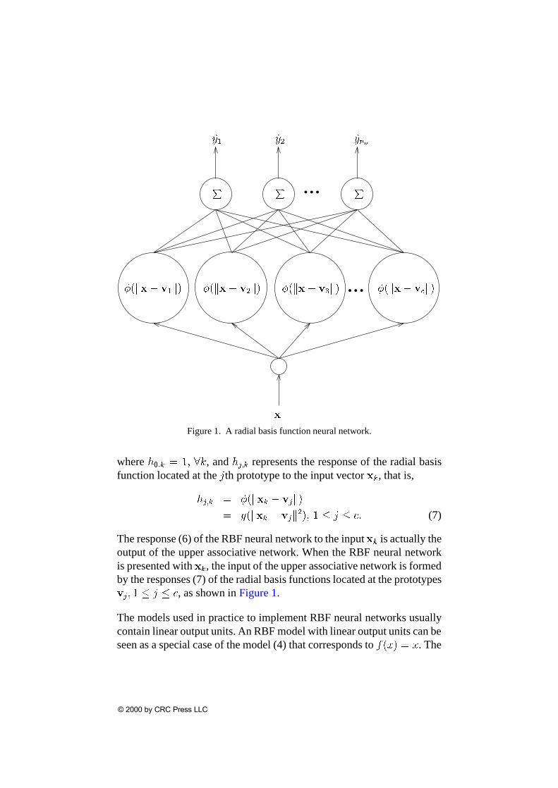
and�(�) is a radial basis function. In such a case, the response of thenetwork to the input vectorxk is:
whereh0;k = 1; 8k, andhj;k represents the response of the radial basisfunction located at thejth prototype to the input vectorxk, that is,
hj;k = �(kxk � vjk)
= g(kxk � vjk2); 1 � j � c: (7)
The response (6) of the RBF neural network to the inputxk is actually theoutput of the upper associative network. When the RBF neural networkis presented withxk, the input of the upper associative network is formedby the responses (7) of the radial basis functions located at the prototypesvj; 1 � j � c, as shown in Figure1.
The models used in practice to implement RBF neural networks usuallycontain linear output units. An RBF model with linear output units can beseen as a special case of the model (4) that corresponds tof(x) = x. The
choice of linear output units was mainly motivated by the hybrid learningschemes originally developed for training RBF neural networks. Never-theless, the learning process is only slightly affected by the form off(�)if RBF neural networks are trained using learning algorithms based ongradient descent. Moreover, the form of an admissible functionf(�) doesnot affect the function approximation capability of the model (4) or theconditions that must be satisfied by radial basis functions. Finally, the useof a nonlinear sigmoidal functionf(�) could make RBF models strongercompetitors to traditional feed-forward neural networks in certain appli-cations, such as those involving pattern classification.
3 Reformulating Radial BasisNeural Networks
A RBF neural network is often interpreted as a composition of localizedreceptive fields. The locations of these receptive fields are determined bythe prototypes while their shapes are determined by the radial basis func-tions used. The interpretation often associated with RBF neural networksimposes some implicit constraints on the selection of radial basis func-tions. For example, RBF neural networks often employ decreasing Gaus-sian radial basis functions despite the fact that there exist both increasingand decreasing radial basis functions. The “neural” interpretation of themodel (4) can be the basis of a systematic search for radial basis func-tions to be used for reformulating RBF neural networks [13], [17], [20],[21]. Such a systematic search is based on mathematical restrictions im-posed on radial basis functions by their role in the formation of receptivefields.
The interpretation of a RBF neural network as a composition of receptivefields requires that the responses of all radial basis functions to all inputsare always positive. If the prototypes are interpreted as the centers of re-ceptive fields, it is required that the response of any radial basis functionbecomes stronger as the input approaches its corresponding prototype.Finally, it is required that the response of any radial basis function be-comes more sensitive to an input vector as this input vector approachesits corresponding prototype.
Lethj;k = g (kxk � vjk2) be the response of thejth radial basis function
of a RBF neural network to the inputxk. According to the above inter-pretation of RBF neural networks, any admissible radial basis function�(x) = g(x2) must satisfy the following three axiomatic requirements[13], [17], [20], [21]:
Axiom 1: hj;k > 0 for all xk 2 X andvj 2 V.
Axiom 2: hj;k > hj;` for all xk;x` 2 X andvj 2 V such thatkxk �vjk
2 < kx` � vjk2.
Axiom 3: If rxkhj;k � @hj;k=@xk denotes the gradient ofhj;k withrespect to the corresponding inputxk, then:
krxkhj;kk2
kxk � vjk2>krx`hj;`k
2
kx` � vjk2;
for all xk;x` 2 X andvj 2 V such thatkxk � vjk2 <
kx` � vjk2.
These basic axiomatic requirements impose some rather mild mathemat-ical restrictions on the search for admissible radial basis functions. Nev-ertheless, this search can be further restricted by imposing additional re-quirements that lead to stronger mathematical conditions. For example,it is reasonable to require that the responses of all radial basis functionsto all inputs are bounded, i.e.,hj;k < 1; 8j; k. On the other hand, thethird axiomatic requirement can be made stronger by requiring that:
and the third axiomatic requirement is satisfied. This implies that condi-tion (8) is stronger than that imposed by the third axiomatic requirement.
The above discussion suggests two complementary axiomatic require-ments for radial basis functions [17]:
Axiom 4: hj;k <1 for all xk 2 X andvj 2 V.
Axiom 5: If rxkhj;k � @hj;k=@xk denotes the gradient ofhj;k withrespect to the corresponding inputxk, then:
krxkhj;kk2 > krx`hj;`k
2;
for all xk;x` 2 X andvj 2 V such thatkxk � vjk2 <
kx` � vjk2.
The selection of admissible radial basis functions can be facilitated bythe following theorem [17]:
Theorem 1:The model described by equation (4) represents a RBF neuralnetwork in accordance with all five axiomatic requirements if and only ifg(�) is a continuous function on(0;1), such that:
1. g(x) > 0; 8x 2 (0;1),
2. g(x) is a monotonically decreasing function ofx 2 (0;1), i.e.,g0(x) < 0; 8x 2 (0;1),
3. g0(x) is a monotonically increasing function ofx 2 (0;1), i.e.,g00(x) > 0; 8x 2 (0;1),
4. limx!0+ g(x) = L, whereL is a finite number.
5. d(x) = g0(x) + 2 x g00(x) > 0; 8x 2 (0;1).
A radial basis function is said to beadmissible in the wide senseif itsatisfies the three basic axiomatic requirements, that is, the first threeconditions of Theorem 1 [13], [17], [20], [21]. If a radial basis func-tion satisfies all five axiomatic requirements, that is, all five conditions ofTheorem 1, then it is said to beadmissible in the strict sense[17].
A systematic search for admissible radial basis functions can be facili-tated by considering basis functions of the form�(x) = g(x2), with g(�)
defined in terms of agenerator functiong0(�) as g(x) = (g0(x))1
1�m ,m 6= 1 [13], [17], [20], [21]. The selection of generator functions thatlead to admissible radial basis functions can be facilitated by the follow-ing theorem [17]:
Theorem 2:Consider the model (4) and letg(x) be defined in terms ofthe generator functiong0(x) that is continuous on(0;1) as:
g(x) = (g0(x))1
1�m ; m 6= 1: (11)
If m > 1, then this model represents a RBF neural network in accordancewith all five axiomatic requirements if:
1. g0(x) > 0; 8x 2 (0;1),
2. g0(x) is a monotonically increasing function ofx 2 (0;1), i.e.,g00(x) > 0; 8x 2 (0;1),
Any generator function that satisfies the first three conditions of Theo-rem 2 leads to admissible radial basis functions in the wide sense [13],[17], [20], [21]. Admissible radial basis functions in the strict sense canbe obtained from generator functions that satisfy all five conditions ofTheorem 2 [17].
4 Admissible Generator Functions
This section investigates the admissibility in the wide and strict sense oflinear and exponential generator functions.
4.1 Linear Generator Functions
Consider the functiong(x) = (g0(x))1
1�m , with g0(x) = a x + b andm > 1. Clearly,g0(x) = a x + b > 0; 8x 2 (0;1), for all a > 0 andb � 0. Moreover,g0(x) = a x+ b is a monotonically increasing functionif g00(x) = a > 0. Forg0(x) = a x + b, g00(x) = a, g000(x) = 0, and
r0(x) =m
m� 1a2: (12)
If m > 1, thenr0(x) > 0; 8x 2 (0;1). Thus,g0(x) = a x + b is anadmissible generator function in the wide sense (i.e., in the sense that itsatisfies the three basic axiomatic requirements) for alla > 0 andb � 0.Certainly, all combinations ofa > 0 andb > 0 also lead to admissiblegenerator functions in the wide sense.
Forg0(x) = a x+ b, the fourth axiomatic requirement is satisfied if:
limx!0+
g0(x) = b > 0: (13)
Forg0(x) = a x+ b,
d0(x) = (a x+ b) a� 2 xm
m� 1a2: (14)
If m > 1, the fifth axiomatic requirement is satisfied ifd0(x) < 0; 8x 2(0;1). Fora > 0, the conditiond0(x) < 0 is satisfied byg0(x) = a x+bif:
Sincem > 1, the fifth axiomatic requirement is satisfied only ifb = 0 or,equivalently, ifg0(x) = a x. However, the valueb = 0 violates the fourthaxiomatic requirement. Thus, there exists no combination ofa > 0 andb > 0 leading to an admissible generator function in the strict sense thathas the formg0(x) = a x+ b.
If a = 1 andb = 2, then the linear generator functiong0(x) = a x + b
becomesg0(x) = x+ 2. For this generator function,g(x) = (x+ 2)1
1�m .If m = 3, g(x) = (x + 2)�
12 corresponds to the inverse multiquadratic
radial basis function:
�(x) = g(x2) =1
(x2 + 2)12
: (16)
For g0(x) = x + 2, limx!0+ g0(x) = 2 and limx!0+ g(x) = 2
1�m .Sincem > 1, g(�) is a bounded function if takes nonzero values. How-ever, the bound ofg(�) increases and approaches infinity as decreasesand approaches 0. Ifm > 1, the conditiond0(x) < 0 is satisfied byg0(x) = x + 2 if:
x >m� 1
m+ 1 2: (17)
Clearly, the fifth axiomatic requirement is satisfied only for = 0, whichleads to an unbounded functiong(�) [13], [20], [21].
Another useful generator function for practical applications can be ob-tained fromg0(x) = a x + b by selectingb = 1 anda = Æ > 0. Forg0(x) = 1 + Æ x, limx!0+ g(x) = limx!0+ g0(x) = 1. For this choiceof parameters, the corresponding radial basis function�(x) = g(x2) isbounded by 1, which is also the bound of the Gaussian radial basis func-tion. If m > 1, the conditiond0(x) < 0 is satisfied byg0(x) = 1 + Æ xif:
x >m� 1
m+ 1
1
Æ: (18)
For a fixedm > 1, the fifth axiomatic requirement is satisfied in the limitÆ !1. Thus, a reasonable choice forÆ in practical situations isÆ � 1.
The radial basis function that corresponds to the linear generator functiong0(x) = a x + b and some value ofm > 1 can also be obtained from the
decreasing functiong0(x) = 1=(a x + b) combined with an appropriatevalue ofm < 1. As an example, form = 3, the generator functiong0(x) = a x + b leads tog(x) = (a x + b)�
12 . For a = 1 and b =
2, this generator function corresponds to the multiquadratic radial basisfunction (16). The multiquadratic radial basis function (16) can also beobtained using the decreasing generator functiong0(x) = 1=(x+ 2)withm = �1. In general, the functiong(x) = (g0(x))
11�m corresponding to
the increasing generator functiong0(x) = a x + b andm = mi > 1,is identical with the functiong(x) = (g0(x))
11�m corresponding to the
decreasing functiong0(x) = 1=(a x+ b) andm = md if:
1
1�mi
=1
md � 1; (19)
or, equivalently, if:mi +md = 2: (20)
Sincemi > 1, (20) implies thatmd < 1.
The admissibility of the decreasing generator functiong0(x) = 1=(a x+b) can also be verified by using directly the results of Theorem 2. Con-sider the functiong(x) = (g0(x))
11�m , with g0(x) = 1=(a x + b) and
m < 1. For alla > 0 andb > 0, g0(x) = 1=(a x+ b) > 0; 8x 2 (0;1).Sinceg00(x) = �a=(a x + b)2 < 0; 8x 2 (0;1), g0(x) = 1=(a x + b)is a monotonically decreasing function for alla > 0. Sinceg000(x) =2a2=(a x+ b)3,
r0(x) =2�m
m� 1
a2
(a x+ b)4: (21)
For m < 1, r0(x) < 0; 8x 2 (0;1), andg0(x) = 1=(a x + b) is anadmissible generator function in the wide sense.
Forg0(x) = 1=(a x+ b),
limx!0+
g0(x) =1
b; (22)
which implies thatg0(x) = 1=(a x+ b) satisfies the fourth axiomatic re-quirement unlessb approaches 0. In such a case,limx!0+ g0(x) = 1=b =
It must be emphasized that both increasing and decreasing exponentialgenerator functions essentially lead to the same radial basis function. Ifm > 1, the increasing exponential generator functiong0(x) = exp(�x),� > 0, corresponds to the Gaussian radial basis function�(x) = g(x2) =exp(�x2=�2), with �2 = (m� 1)=�. If m < 1, the decreasing exponen-tial generator functiong0(x) = exp(��x), � > 0, also corresponds tothe Gaussian radial basis function�(x) = g(x2) = exp(�x2=�2), with�2 = (1 � m)=�. In fact, the functiong(x) = (g0(x))
11�m correspond-
ing to the increasing generator functiong0(x) = exp(�x); � > 0, withm = mi > 1 is identical with the functiong(x) = (g0(x))
11�m corre-
sponding to the decreasing functiong0(x) = exp(��x); � > 0, withm = md < 1 if:
mi � 1 = 1�md; (33)
or, equivalently, if:mi +md = 2: (34)
5 Selecting Generator Functions
All possible generator functions considered in the previous section sat-isfy the three basic axiomatic requirements but none of them satisfiesall five axiomatic requirements. In particular, the fifth axiomatic require-ment is satisfied only by generator functions of the formg0(x) = a x,which violate the fourth axiomatic requirement. Therefore, it is clear thatat least one of the five axiomatic requirements must be compromised inorder to select a generator function. Since the response of the radial basisfunctions must be bounded in some function approximation applications,generator functions can be selected by compromising the fifth axiomaticrequirement. Although this requirement is by itself very restrictive, itsimplications can be used to guide the search for generator functions ap-propriate for gradient descent learning [17].
The norm of the gradientrxkhj;k can be obtained from (35) as:
krxkhj;kk2 = 4 kxk � vjk
2�g0(kxk � vjk
2)�2
= 4 t(kxk � vjk2); (36)
wheret(x) = x (g0(x))2. According to Theorem 1, the fifth axiomaticrequirement is satisfied if and only ifd(x) = g0(x)+2 x g00(x) > 0; 8x 2(0;1). Sincet(x) = x (g0(x))2,
t0(x) = g0(x) (g0(x) + 2 x g00(x))
= g0(x) d(x): (37)
Theorem 1 requires thatg(x) is a decreasing function ofx 2 (0;1),which implies thatg0(x) < 0; 8x 2 (0;1). Thus, (37) indicates thatthe fifth axiomatic requirement is satisfied ift0(x) < 0; 8x 2 (0;1).If this condition is not satisfied, thenkr
xkhj;kk
2 is not a monotonicallydecreasing function ofkxk � vjk
2 in the interval(0;1), as requiredby the fifth axiomatic requirement. Given a functiong(�) satisfying thethree basic axiomatic requirements, the fifth axiomatic requirement canbe relaxed by requiring thatkr
xkhj;kk
2 is a monotonically decreasingfunction of kxk � vjk
2 in the interval(B;1) for someB > 0. Ac-cording to (36), this is guaranteed if the functiont(x) = x (g0(x))2
has a maximum atx = B or, equivalently, if there exists aB > 0such thatt0(B) = 0 and t00(B) < 0. If B 2 (0;1) is a solutionof t0(x) = 0 and t00(B) < 0, then t0(x) > 0; 8x 2 (0; B), andt0(x) < 0; 8x 2 (B;1). Thus,krxkhj;kk
2 is an increasing functionof kxk � vjk
2 for kxk � vjk2 2 (0; B) and a decreasing function of
kxk � vjk2 for kxk � vjk2 2 (B;1). For all input vectorsxk that sat-
isfy kxk � vjk2 < B, the norm of the gradientrxkhj;k correspondingto thejth radial basis function decreases asxk approaches its center thatis located at the prototypevj. This is exactly the opposite behavior ofwhat would intuitively be expected, given the interpretation of radial ba-sis functions as receptive fields. As far as gradient descent learning isconcerned, the hypersphereRB = fx 2 X � IRni : kx� vk2 2 (0; B)gis a “blind spot” for the radial basis function located at the prototypev.The blind spot provides a measure of the sensitivity of radial basis func-tions to input vectors close to their centers.
The blind spotRBlincorresponding to the linear generator function
The effect of the parameterm to the size of the blind spot is revealed bythe behavior of the ratio(m�1)=(m+1) viewed as a function ofm. Since(m � 1)=(m + 1) increases as the value ofm increases, increasing thevalue ofm expands the blind spot. For a fixed value ofm > 1, Blin = 0only if b = 0. For b 6= 0, Blin decreases and approaches 0 asa increasesand approaches infinity. Ifa = 1 andb = 2, Blin approaches 0 as approaches 0. Ifa = Æ andb = 1, Blin decreases and approaches 0 asÆincreases and approaches infinity.
The blind spotRBexpcorresponding to the exponential generator function
g0(x) = exp(�x) is determined by:
Bexp =m� 1
2�: (39)
For a fixed value of�, the blind spot depends exclusively on the param-eterm. Once again, the blind spot corresponding to the exponential gen-erator function expands as the value ofm increases. For a fixed value ofm > 1, Bexp decreases and approaches 0 as� increases and approaches
infinity. For g0(x) = exp(�x), g(x) = (g0(x))1
1�m = exp(�x=�2) with�2 = (m � 1)=�. As a result, the blind spot corresponding to the expo-nential generator function approaches 0 only if the width of the Gaussianradial basis function�(x) = g(x2) = exp(�x2=�2) approaches 0. Sucha range of values of� would make it difficult for Gaussian radial ba-sis functions to behave as receptive fields that can cover the entire inputspace.
It is clear from (38) and (39) that the blind spot corresponding to theexponential generator function is much more sensitive to changes ofmcompared with that corresponding to the linear generator function. Thiscan be quantified by computing for both generator functions the relativesensitivity ofB = B(m) in terms ofm, defined as:
For the linear generator functiong0(x) = a x + b, @Blin=@m =(2=(m+ 1)2) (b=a) and
SmBlin
=2m
m2 � 1: (41)
For the exponential generator functiong0(x) = exp(�x), @Bexp=@m =1=(2 �) and
SmBexp
=m
m� 1: (42)
Combining (41) and (42) gives:
SmBexp
=m + 1
2SmBlin
: (43)
Sincem > 1, SmBexp
> SmBlin
. As an example, form = 3 the sensitiv-ity with respect tom of the blind spot corresponding to the exponen-tial generator function is twice that corresponding to the linear generatorfunction.
5.2 Criteria for Selecting Generator Functions
The response of the radial basis function located at the prototypevj totraining vectors depends on their Euclidean distance fromvj and theshape of the generator function used. If the generator function does notsatisfy the fifth axiomatic requirement, the response of the radial basisfunction located at each prototype exhibits the desired behavior only ifthe training vectors are located outside its blind spot. This implies thatthe training of a RBF model by a learning procedure based on gradientdescent depends mainly on the sensitivity of the radial basis functions totraining vectors outside their blind spots. This indicates that the criteriaused for selecting generator functions should involve both the shapes ofthe radial basis functions relative to their blind spots and the sensitivityof the radial basis functions to input vectors outside their blind spots.The sensitivity of the responsehj;k of thejth radial basis function to anyinputxk can be measured by the norm of the gradientrxkhj;k. Thus, theshape and sensitivity of the radial basis function located at the prototypevj are mainly affected by:
1. the valueh�j = g(B) of the responsehj;k = g(kxk � vjk2) of the
jth radial basis function atkxk � vjk2 = B and the rate at whichhj;k = g(kxk � vjk
2) decreases askxk � vjk2 increases aboveBand approaches infinity, and
2. the maximum value attained by the norm of the gradientrxkhj;kat kxk � vjk2 = B and the rate at whichkrxkhj;kk
2 decreases askxk � vjk
2 increases aboveB and approaches infinity.
The criteria that may be used for selecting radial basis functions can beestablished by considering the following extreme situation. Suppose theresponsehj;k = g(kxk�vjk
2) diminishes very quickly and the receptivefield located at the prototypevj does not extend far beyond the blind spot.This can have a negative impact on the function approximation ability ofthe corresponding RBF model since the region outside the blind spot con-tains the input vectors that affect the implementation of the input-outputmapping as indicated by the sensitivity measurekrxkhj;kk
2. Thus, a gen-erator function must be selected in such a way that:
1. the responsehj;k and the sensitivity measurekrxkhj;kk2 take sub-
stantial values outside the blind spot before they approach 0, and
2. the responsehj;k is sizable outside the blind sport even after thevalues ofkrxkhj;kk
2 become negligible.
The rate at which the responsehj;k = g(kxk � vjk2) decreases relates
to the “tails” of the functionsg(�) that correspond to different generatorfunctions. The use of a short-tailed functiong(�) shrinks the receptivefields of the RBF model while the use of a long-tailed functiong(�) in-creases the overlapping between the receptive fields located at differentprototypes. Ifg(x) = (g0(x))
11�m andm > 1, the tail ofg(x) is deter-
mined by how fast the corresponding generator functiong0(x) changesas a function ofx. As x increases, the exponential generator functiong0(x) = exp(�x) increases faster than the linear generator functiong0(x) = a x + b. As a result, the responseg(x) = (g0(x))
11�m dimin-
ishes quickly ifg0(�) is exponential and slower ifg0(�) is linear.
The behavior of the sensitivity measurekrxkhj;kk2 also depends on the
properties of the functiong(�). Forhj;k = g(kxk�vjk2),rxkhj;k can be
Figure 3. The responsehj;k = g(kxk � vjk2) of thejth radial basis function
and the norm of the gradientkrxkhj;kk
2 plotted as functions ofkxk �vjk2 for
g(x) = (g0(x))1
1�m , with g0(x) = 1 + Æ x, m = 3, andÆ = 100.
kxk�vjk2 increases from 0 toB = 1=(2 Æ) and decreases monotonically
askxk�vjk2 increasesaboveB and approaches infinity. Figures2 and 3indicate that, regardless of the value ofÆ, the responsehj;k of the radialbasis function located at the prototypevj is sizable outside the blind spoteven after the values ofkrxkhj;kk
2 become negligible. Thus, the radialbasis function located at the prototypevj is activated by all input vectorsthat correspond to substantial values ofkrxkhj;kk
2.
5.3.2 Exponential Generator Functions
If g(x) = (g0(x))1
1�m , with g0(x) = exp(�x) andm > 1, the responsehj;k = g(kxk � vjk
2) of thejth radial basis function toxk is:
hj;k = exp
�kxk � vjk
2
�2
!; (52)
where �2 = (m � 1)=�. For this generator function,g00(x) =� exp(�x) = � g0(x). In this case,g00 (kxk � vjk
Figure 5. The responsehj;k = g(kxk � vjk2) of thejth radial basis function
and the norm of the gradientkrxkhj;kk
2 plotted as functions ofkxk �vjk2 for
g(x) = (g0(x))1
1�m , with g0(x) = exp(� x), m = 3, and� = 10.
aboveB and approaches infinity. Nevertheless, there are some signifi-cant differences between the responsehj;k and the sensitivity measurekrxkhj;kk
2 corresponding to linear and exponential generator functions.If g0(x) = exp(�x), then the responsehj;k is substantial for the inputvectors inside the blind spot but diminishes very quickly for values ofkxk � vjk
2 aboveB. In fact, the values ofhj;k become negligible evenbeforekrxkhj;kk
2 approaches asymptotically zero values. This is in di-rect contrast with the behavior of the same quantities corresponding tolinear generator functions, which are shown in Figures 2 and 3.
6 Learning Algorithms Based on GradientDescent
Reformulated RBF neural networks can be trained to mapxk 2 IRni intoyk = [y1;k y2;k : : : yno;k]
T 2 IRno, where the vector pairs(xk;yk); 1 �k � M , form the training set. Ifxk 2 IRni is the input to a reformulatedRBF network, its response isyk = [y1;k y2;k : : : yno;k]
T . Training is typicallybased on the minimization of the error between the actual outputs of thenetworkyk; 1 � k �M , and the desired responsesyk; 1 � k �M .
6.1 Batch Learning Algorithms
A reformulated RBF neural network can be trained by minimizing theerror:
E =1
2
MXk=1
noXi=1
(yi;k � yi;k)2: (56)
Minimization of (56) using gradient descent implies that all training ex-amples are presented to the RBF network simultaneously. Such trainingstrategy leads tobatchlearning algorithms. The update equation for theweight vectors of the upper associative network can be obtained usinggradient descent as [21]:
�wp = ��rwpE
= �MXk=1
"op;k hk; (57)
where� is the learning rate and"op;k is theoutput error, given as:
"op;k = f 0(�yp;k) (yp;k � yp;k): (58)
Similarly, the update equation for the prototypes can be obtained usinggradient descent as [21]:
where� is the learning rate and"hq;k is thehidden error, defined as:
"hq;k = �q;k
noXi=1
"oi;k wiq; (60)
with �q;k = �2 g0 (kxk � vqk
2). The selection of a specific functiong(�)influences the update of the prototypes through�q;k = �2 g
0(kxk�vqk2),
which is involved in the calculation of the corresponding hidden error"hq;k. Sincehq;k = g (kxk � vqk
2) andg(x) = (g0(x))1
1�m , �q;k is givenby (48) and the hidden error (60) becomes:
"hq;k =2
m� 1(hq;k)
m g00(kxk � vqk2)
noXi=1
"oi;k wiq: (61)
A RBF neural network can be trained according to the algorithm pre-sented above in a sequence ofadaptation cycles, where an adaptationcycle involves the update of all adjustable parameters of the network. Anadaptation cycle begins by replacing the current estimate of each weightvectorwp; 1 � p � no, by its updated version:
wp +�wp = wp + �MXk=1
"op;k hk: (62)
Given the learning rate� and the responseshk of the radial basis func-tions, these weight vectors are updated according to the output errors"op;k; 1 � p � no. Following the update of these weight vectors, the cur-rent estimate of each prototypevq, 1 � q � c, is replaced by:
vq +�vq = vq + �MXk=1
"hq;k (xk � vq): (63)
For a given value of the learning rate�, the update ofvq depends on thehidden errors"hq;k; 1 � k �M . The hidden error"hq;k is influenced by theoutput errors"oi;k; 1 � i � no, and the weightswiq; 1 � i � no, throughthe term
Pnoi=1 "
oi;k wiq. Thus, the RBF neural network is trained according
to this scheme by propagating back the output error.
This algorithm can be summarized as follows:
1. Select� and�; initialize fwijg with zero values; initialize the pro-totypesvj; 1 � j � c; seth0;k = 1; 8k.
Reformulated RBF neural networks can also be trained “on-line” byse-quentiallearning algorithms. Such algorithms can be developed by usinggradient descent to minimize the errors:
for k = 1; 2; : : : ;M . The update equation for the weight vectors of theupper associative network can be obtained using gradient descent as [21]:
�wp;k = wp;k �wp;k�1
= ��rwpEk
= � "op;k hk; (65)
wherewp;k�1 andwp;k are the estimates of the weight vectorwp be-fore and after the presentation of the training example(xk;yk), � is thelearning rate, and"op;k is the output error defined in (58). Similarly, theupdate equation for the prototypes can be obtained using gradient descentas [21]:
�vq;k = vq;k � vq;k�1
= ��rvqEk
= � "hq;k (xk � vq); (66)
wherevq;k�1 andvq;k are the estimates of the prototypevq before andafter the presentation of the training example(xk;yk), � is the learningrate, and"hq;k is the hidden error defined in (61).
When an adaptation cycle begins, the current estimates of the weightvectorswp and the prototypesvq are stored inwp;0 andvq;0, respectively.After an example(xk;yk); 1 � k � M , is presented to the network, eachweight vectorwp; 1 � p � no, is updated as:
wp;k = wp;k�1 +�wp;k = wp;k�1 + � "op;k hk: (67)
Following the update of all the weight vectorswp; 1 � p � no, eachprototypevq; 1 � q � c, is updated as:
An adaptation cycle is completed in this case after the sequential pre-sentation to the network of all the examples included in the training set.Once again, the RBF neural network is trained according to this schemeby propagating back the output error.
This algorithm can be summarized as follows:
1. Select� and�; initialize fwijg with zero values; initialize the pro-totypesvj; 1 � j � c; seth0;k = 1; 8k.
5. Update the adjustable parameters for allk = 1; 2; : : : ;M :
� "oi;k = f 0(�yi;k)(yi;k � yi;k); 8i.
� wi wi + � "oi;k hk; 8i.
� "hj;k =2
m�1g00 (kxk � vjk
2) (hj;k)m Pno
i=1 "oi;k wij; 8j.
� vj vj + � "hj;k (xk � vj); 8j.
6. Compute the current response:
� hj;k = (g0 (kxk � vjk2))
11�m ; 8j; k.
� hk = [h0;k h1;k : : : hc;k]T ; 8k.
� yi;k = f(wTi hk); 8i; k.
7. ComputeE = 12
PMk=1
Pnoi=1(yi;k � yi;k)
2.
8. If: (Eold � E)=Eold > �; then: go to 4.
6.3 Initialization of Supervised Learning
The training of reformulated RBF neural networks using gradient de-scent can be initialized by randomly generating the set of prototypes thatdetermine the locations of the radial basis function centers in the inputspace. Such an approach relies on the supervised learning algorithm todetermine appropriate locations for the radial basis function centers byupdating the prototypes during learning. Nevertheless, the training of re-formulated RBF neural networks by gradient descent algorithms can befacilitated by initializing the supervised learning process using a set ofprototypes specifically determined to represent the input vectors included
in the training set. This can be accomplished by computing the initial setof prototypes using unsupervised clustering or learning vector quantiza-tion (LVQ) algorithms.
According to the learning scheme often used for training conventionalRBF neural networks [34], the locations of the radial basis function cen-ters are determined from the input vectors included in the training setusing thec-means (ork-means) algorithm. Thec-means algorithm be-gins from an initial set ofc prototypes, which implies the partition of theinput vectors intoc clusters. Each cluster is represented by a prototype,which is evaluated at subsequent iterations as the centroid of the inputvectors belonging to that cluster. Each input vector is assigned to thecluster whose prototype is its closest neighbor. In mathematical terms,the indicator functionuij = uj(xi) that assigns the input vectorxi to thejth cluster is computed as [9]:
For a given set of indicator functions, the new set of prototypes is calcu-lated as [9]:
vj =
PMi=1 uij xiPMi=1 uij
; 1 � j � c: (70)
The c-means algorithm partitions the input vectors into clusters repre-sented by a set of prototypes based onhard or crisp decisions. In otherwords, each input vector is assigned to the cluster represented by its clos-est prototype. Since this strategy fails to quantify the uncertainty typi-cally associated with partitioning a set of input vectors, the performanceof thec-means algorithm depends rather strongly on its initialization [8],[26]. When this algorithm is initialized randomly, it often converges toshallow local minima and produces empty clusters.
Most of the disadvantages of thec-means algorithm can be overcomeby employing a prototype splitting procedure to produce the initial setof prototypes. Such a procedure is employed by a variation of thec-means algorithm often referred to in the literature as the LBG (Linde-Buzo-Gray) algorithm [31], which is often used for codebook design inimage and video compression approaches based on vector quantization.
The LBG algorithm employs an initialization scheme to compensate forthe dependence of thec-means algorithm on its initialization [8]. Morespecifically, this algorithm generates the desired number of clusters bysuccessively splitting the prototypes and subsequently employing thec-means algorithm. The algorithm begins with a single prototype that iscalculated as the centroid of the available input vectors. This prototype issplit into two vectors, which provide the initial estimate for thec-meansalgorithm that is used withc = 2. Each of the resulting vectors is thensplit into two vectors and the above procedure is repeated until the de-sired number of prototypes is obtained. Splitting is performed by addingthe perturbation vectors�ei to each vectorvi producing two vectors:vi+ei andvi�ei. The perturbation vectorei can be calculated from thevariance between the input vectors and the prototypes [8].
7 Generator Functions and GradientDescent Learning
The effect of the generator function on gradient descent learning al-gorithms developed for reformulated RBF neural networks essentiallyrelates to the criteria established in Section 5 for selecting generatorfunctions. These criteria were established on the basis of the responsehj;k of the jth radial basis function to an input vectorxk and the normof the gradientr
xkhj;k, that can be used to measure the sensitivity
of the radial basis function responsehj;k to an input vectorxk. Sincerxkhj;k = �rvjhj;k, (46) gives
krvjhj;kk2 = kxk � vjk
2 �2j;k: (71)
According to (71), the quantitykxk � vjk2 �2j;k can also be used to mea-
sure the sensitivity of the response of thejth radial basis function tochanges in the prototypevj that represents its location in the input space.
The gradient descent learning algorithms presented in Section 6 attemptto train a RBF neural network to implement a desired input-output map-ping by producing incremental changes of its adjustable parameters, i.e.,the output weights and the prototypes. If the responses of the radial ba-sis functions are not substantially affected by incremental changes of theprototypes, then the learning process reduces to incremental changes of
the output weights and eventually the algorithm trains a single-layeredneural network. Given the limitations of single-layered neural networks[28], such updates alone are unlikely to implement non-trivial input-output mappings. Thus, the ability of the network to implement a desiredinput-output mapping depends to a large extent on the sensitivity of theresponses of the radial basis functions to incremental changes of theircorresponding prototypes. This discussion indicates that the sensitivitymeasurekrvjhj;kk
2 is relevant to gradient descent learning algorithmsdeveloped for reformulated RBF neural networks. Moreover, the form ofthis sensitivity measure in (71) underlines the significant role of the gen-erator function, whose selection affectskrvjhj;kk
2 as indicated by thedefinition of�j;k in (48). The effect of the generator function on gradientdescent learning is revealed by comparing the responsehj;k and the sen-sitivity measurekrvjhj;kk
2 = krxkhj;kk2 corresponding to the linear
and exponential generator functions.
According to Figures 2 and 3, the response hj;k of the jth radial basisfunction to the inputxk diminishes very slowly outside the blind spot,i.e., askxk � vjk2 increases aboveB. This implies that the training vec-tor xk has a non-negligible effect on the responsehj;k of the radial basisfunction located at this prototype. The behavior of the sensitivity mea-surekrvjhj;kk
2 outside the blind spot indicates that the update of theprototypevj produces significant variations in the input of the upper as-sociative network, which is trained to implement the desired input-outputmapping by updating theoutput weights. Figures 2and 3 also reveal thetrade-off involved in the selection of the free parameterÆ in practice. Asthe value ofÆ increases,krvjhj;kk
2 attains significantly higher values.This implies that thejth radial basis function is more sensitive to up-dates of the prototypevj due to input vectors outside its blind spot. Theblind spot shrinks as the value ofÆ increases butkr
vjhj;kk
2 approaches0 quickly outside the blind spot, i.e., as the value ofkxk�vjk2 increasesaboveB. This implies that the receptive fields located at the prototypesshrink, which can have a negative impact on the gradient descent learn-ing. Increasing the value ofÆ can also affect the number of radial ba-sis functions required for the implementation of the desired input-outputmapping. This is due to the fact that more radial basis functions are re-quired to cover the input space. The receptive fields located at the proto-types can be expanded by decreasing the value ofÆ. However,krvjhj;kk
becomes flat as the value ofÆ decreases. This implies that very small val-ues ofÆ can decrease the sensitivity of the radial basis functions to theinput vectors included in their receptive fields.
According to Figures 4 and 5, the response of the jth radial basis func-tion to the inputxk diminishes very quickly outside the blind spot, i.e.,askxk � vjk2 increases aboveB. This behavior indicates that if a RBFnetwork is constructed using exponential generator functions, the inputsxk corresponding to high values ofkrvjhj;kk
2 have no significant effecton the response of the radial basis function located at the prototypevj.As a result, the update of this prototype due toxk does not produce sig-nificant variations in the input of the upper associative network that im-plements the desired input-output mapping. Figures 4 and 5 also indicatethat the blind spot shrinks as the value of� increases whilekrvjhj;kk
2
reaches higher values. Decreasing the value of� expands the blind spotbutkr
vjhj;kk
2 reaches lower values. In other words, the selection of thevalue of� in practice involves a trade-off similar to that associated withthe selection of the free parameterÆ when the radial basis functions areformed by linear generator functions.
8 Handwritten Digit Recognition
8.1 The NIST Databases
Reformulated RBF neural networks were tested and compared with com-peting techniques on a large-scale handwritten digit recognition problem.The objective of a classifier in this application is the recognition of thedigit represented by a binary image of a handwritten numeral. Recogni-tion of handwritten digits is the key component of automated systems de-veloped for a great variety of real-world applications, including mail sort-ing and check processing. Automated recognition of handwritten digits isnot a trivial task due to the high variance of handwritten digits caused bydifferent writing styles, pens, etc. Thus, the development of a reliable sys-tem for handwritten digit recognition requires large databases containinga great variety of samples. Such a collection of handwritten digits is con-tained in theNIST Special Databases 3, which contain about 120000isolated binary digits that have been extracted from sample forms. These
Figure 6. Digits from the NIST Databases: (a) original binary images, (b)32�32binary images after one stage of preprocessing (slant and size normalization),and (c)16� 16 images of the digits after two stages of preprocessing (slant andsize normalization followed by wavelet decomposition).
digits were handwritten by about 2100 field representatives of the UnitedStates Census Bureau. The isolated digits were scanned to produce bi-nary images of size40 � 60 pixels, which are centered in a128 � 128box. Figure 6(a) shows some sample digits from 0 to 9 from the NISTdatabases used in these experiments. The data set was partitioned in threesubsets as follows: 58646 digits were used for training, 30367 digits wereused for testing, and the remaining 30727 digits constituted the validationset.
8.2 Data Preprocessing
The raw data from the NIST databases were preprocessed in order to re-duce the variance of the images that is not relevant to classification. Thefirst stage of the preprocessing scheme produced a slant and size nor-malized version of each digit. The slant of each digit was found by firstdetermining its center of gravity, which defines an upper and lower halfof it. The centers of gravity of each half were subsequently computedand provided an estimate of the vertical main axis of the digit. This axiswas then made exactly vertical using a horizontal shear transformation.In the next step, the minimal bounding box was determined and the digitwas scaled into a32 � 32 box. This scaling may slightly distort the as-pect ratio of the digits by centering, if necessary, the digits in the box.Figure 6(b) shows the same digits shown in Figure 6(a) after slant andsize normalization.
The second preprocessing stage involved a 4-level wavelet decomposi-tion of the32� 32 digit representation produced by the first preprocess-ing stage. Each decomposition level includes the application of a 2-DHaar wavelet filter in the decomposed image, followed by downsamplingby a factor of 2 along the horizontal and vertical directions. Becauseof downsampling, each decomposition level produces four subbands oflower resolution, namely a subband that carries background information(containing the low-low frequency components of the original subband),two subbands that carry horizontal and vertical details (containing low-high and high-low frequency components of the original subband), and asubband that carries diagonal details (containing the high-high frequencycomponents of the original subband). As a result, the 4-level decompo-sition of the original32 � 32 image produced three subbands of sizes16� 16, 8� 8, and4� 4, and four subbands of size2� 2. The32� 32image produced by wavelet decomposition was subsequently reduced toan image of size16� 16 by representing each2� 2 window by the aver-age of the four pixels contained in it. This step reduces the amount of databy 3/4 and has a smoothing effect that suppresses the noise present in the32 � 32 image [1]. Figure 6(c) shows the images representing the digitsshown in Figures 6(a) and 6(b), resulting after the second preprocessingstage described above.
8.3 Classification Tools for NIST Digits
This section begins with a brief description of the variants of thek-nearest neighbor(k-NN) classifier used for benchmarking the perfor-mance of the neural networks tested in the experiments and also outlinesthe procedures used for classifying the digits from the NIST databasesusing neural networks. These procedures involve the formation of thedesired input-output mapping and the strategies used to recognize theNIST digits by interpreting the responses of the trained neural networksto the input samples.
Thek-NN classifier uses feature vectors from the training set as a refer-ence to classify examples from the testing set. Given an input examplefrom the testing set, thek-NN classifier computes its Euclidean distancefrom all the examples included in the training set. Thek-NN classifiercan be implemented to classify all input examples (no rejections allowed)
or to selectively reject some ambiguous examples. Thek-NN classifiercan be implemented using two alternative classification strategies: Ac-cording to the first and most frequently used classification strategy, eachof thek closest training examples to the input example has a vote witha weight equal to 1. According to the second classification strategy, theith closest training example to the input example has a vote with weight1=i; that is, the weight of the closest example is 1, the weight of thesecond closest example is1=2, etc. When no rejections are allowed, theclass that receives the largest sum of votes wins the competition and theinput example is assigned the corresponding label. The input exampleis recognizedif the label assigned by the classifier and the actual labelare identical orsubstitutedif the assigned and actual labels are different.When rejections are allowed and thek closest training examples to theinput example have votes equal to 1, the example isrejectedif the largestsum of votes is less thank. Otherwise, the input example is classifiedaccording to the strategy described above.
The reformulated RBF neural networks and feed-forward neural net-works (FFNNs) tested in these experiments consisted of256 = 16� 16inputs and 10 linear output units, each representing a digit from 0 to 9.The inputs of the networks were normalized to the interval[0; 1]. Thelearning rate in all these experiments was� = 0:1. The networks weretrained to respond withyi;k = 1 andyj;k = 0; 8j 6= i, when presentedwith an input vectorxk 2 X corresponding to the digit represented bytheith output unit. The assignment of input vectors to classes was basedon a winner-takes-all strategy. More specifically, each input vector wasassigned to the class represented by the output unit of the trained RBFneural network with the maximum response. In an attempt to improvethe reliability of the neural-network-based classifiers, label assignmentwas also implemented by employing an alternative scheme that allowsthe rejection of some ambiguous digits according to the strategy de-scribed below: Suppose one of the trained networks is presented withan input vectorx representing a digit from the testing or the validationset and letyi; 1 � i � no, be the responses of its output units. Lety(1) = yi1 be the maximum among all responses of the output units, thatis, y(1) = yi1 = maxi2I1fyig, with I1 = f1; 2; : : : ; nog. Let y(2) = yi2be the maximum among the responses of the rest of the output units, thatis, y(2) = yi2 = maxi2I2fyig, with I2 = I1 � fi1g. The simplest classi-
fication scheme would be to assign the digit represented byx to thei1thclass, which implies that none of the digits would be rejected by the net-work. Nevertheless, the reliability of this assignment can be improved bycomparing the responsesy(1) andy(2) of the two output units that claimthe digit for their corresponding classes. If the responsesy(1) and y(2)
are sufficiently close, then the digit represented byx probably lies in aregion of the input space where the classes represented by thei1th andi2th output units overlap. This indicates that the reliability of classifica-tion can be improved by rejecting this digit. This rejection strategy canbe implemented by comparing the difference�y = y(1) � y(2) with arejection parameterr � 0. The digit corresponding tox is acceptedif�y � r and rejectedotherwise. An accepted digit isrecognizedif theoutput unit with the maximum response represents the desired class andsubstitutedotherwise. The rejection rate depends on the selection of therejection parameterr � 0. If r = 0, then the digit corresponding tox isaccepted if�y = y(1) � y(2) � 0, which is by definition true. This im-plies that none of the input digits is rejected by the network ifr = 0. Therejection rate increases as the value of the rejection parameter increasesabove 0.
8.4 Role of the Prototypes in Gradient DescentLearning
RBF neural networks are often trained to implement the desired input-output mapping by updating the output weights, that is, the weights thatconnect the radial basis functions and the output units, in order to min-imize the output error. The radial basis functions are centered at a fixedset of prototypes that define a partition of the input space. In contrast,the gradient descent algorithm presented in Section 6 updates the proto-types representing the centers of the radial basis functions together withthe output weights every time training examples are presented to the net-work. This set of experiments investigated the importance of updating theprototypes during the learning process in order to implement the desiredinput-output mapping. The reformulated RBF neural networks tested inthese experiments containedc = 256 radial basis functions obtained interms of the generator functiong0(x) = 1+Æ x, with g(x) = (g0(x))
11�m ,
m = 3 and Æ = 10. In all these experiments the prototypes of the
Figure 7. Performance of a reformulated RBF neural network tested on thetesting and validation sets during its training. The network was trained (a) byupdating only its output weights, and (b) by updating its output weights andprototypes.
RBF neural networks were determined by employing the initializationscheme described in Section 6, which involves prototype splitting fol-lowed by the c-means algorithm. Figure 7 summarizes the performanceof the networks trained in these experiments at different stages of thelearning process. Figure 7(a) shows the percentage of digits from thetesting and validation sets substituted by the RBF network trained by up-dating only the output weights while keeping the prototypes fixed duringthe learning process. Figure7(b) showsthepercentageof digits from thetesting and validation sets substituted by the reformulated RBF neuralnetwork trained by updating the prototypes and the output weights ac-cording to the sequential gradient descent learning algorithm presentedin Section 6. In both cases, the percentage of substituted digits decreasedwith some fluctuations during the initial adaptation cycles and remainedalmost constant after a certain number of adaptation cycles. When theprototypes were fixed during learning, the percentage of substituted dig-its from both testing and validation sets remained almost constant after1000 adaptation cycles. In contrast, the percentage of substituted digitsdecreased after 1000 adaptation cycles and remained almost constant af-ter 3000 adaptation cycles when the prototypes were updated togetherwith the output weights using gradient descent. In this case, the percent-age of substituted digits reached 1.69% on the testing set and 1.53% onthe validation set. This outcome can be compared with the substitution of3.79% of the digits from the testing set and 3.54% of the digits from thevalidation set produced when the prototypes remained fixed during learn-ing. This experimental outcome verifies that the performance of RBFneural networks can be significantly improved by updating all their freeparameters during learning according to the training set, including theprototypes that represent the centers of the radial basis functions in theinput space.
8.5 Effect of the Number of Radial Basis Functions
This set of experiments evaluated the performance on the testing andvalidation sets formed from the NIST data of various reformulated RBFneural networks at different stages of their training. The reformulatedRBF neural networks containedc = 64, c = 128, c = 256, andc = 512 radial basis functions obtained in terms of the generator func-
Figure 8. Performance of reformulated RBF neural networks with differentnumbers of radial basis functions during their training. The substitution rate wascomputed (a) on the testing set, and (b) on the validation set.
tion g0(x) = 1 + Æ x as�(x) = g(x2), with g(x) = (g0(x))1
1�m , m = 3and Æ = 10. All networks were trained using the sequential gradientdescent algorithm described in Section 6. The initial prototypes werecomputed using the initialization scheme involving prototype splitting.Figures 8(a) and 8(b) plot the percentage of digits from the testing andvalidation sets, respectively, that were substituted by all four reformu-lated RBF neural networks as a function of the number of adaptationcycles. Regardless of the number of radial basis functions contained bythe reformulated RBF neural networks, their performance on both test-ing and validation sets improved as the number of adaptation cycles in-creased. The improvement of the performance was significant during theinitial adaptation cycles, which is consistent with the behavior and con-vergence properties of the gradient descent algorithm used for training.Figures 8(a) and 8(b) also indicate that the number of radial basis func-tions had a rather significant effect on the performance of reformulatedRBF neural networks. The performance of reformulated RBF neural net-works on both testing and validation sets improved as the number ofradial basis functions increased fromc = 64 to c = 128. The best per-formance on both sets was achieved by the reformulated RBF neural net-works containingc = 256 andc = 512 radial basis functions. It mustbe noted that there are some remarkable differences in the performanceof these two networks on the testing and validation sets. According toFigure 8(a), the reformulated RBF neural networks withc = 256 andc = 512 radial basis functions substituted almost the same percentageof digits from the testing set after 1000 adaptation cycles. However, thenetwork withc = 512 radial basis functions performed slightly betteron the testing set than that containingc = 256 radial basis functionswhen the training continued beyond 7000 adaptation cycles. Accordingto Figure 8(b), the reformulated RBF network withc = 256 radial ba-sis functions outperformed consistently the network containingc = 512radial basis functions on the validation set for the first 6000 adaptationcycles. However, the reformulated RBF network withc = 512 radialbasis functions substituted a smaller percentage of digits from the vali-dation set than the network withc = 256 radial basis functions when thetraining continued beyond 7000 adaptation cycles.
Figure 9. Performance of reformulated RBF neural networks with 512 radialbasis functions during their training. The substitution rates were computed onthe training, testing, and validation sets when gradient descent training was ini-tialized (a) randomly, and (b) by prototype splitting.
8.6 Effect of the Initialization of Gradient DescentLearning
This set of experiments evaluated the effect of the initialization of thesupervised learning on the performance of reformulated RBF neural net-works trained by gradient descent. The reformulated RBF neural networktested in these experiments containedc = 512 radial basis functions con-structed as�(x) = g(x2), with g(x) = (g0(x))
11�m , g0(x) = 1 + Æ x,
m = 3, andÆ = 10. The network was trained by the sequential gradi-ent descent algorithm described in Section 6. Figures9(a) and 9(b) showthe percentage of digits from the training, testing, and validation setssubstituted during the training process when gradient descent learningwas initialized by randomly selecting the prototypes and by prototypesplitting, respectively. When the initial prototypes were determined byprototype splitting, the percentage of substituted digits from the trainingset decreased below 1% after 1000 adaptation cycles and reached valuesbelow 0.5% after 3000 adaptation cycles. In contrast, the percentage ofsubstituted digits from the training set decreased much slower and neverreached values below 1% when the initial prototypes were produced by arandom number generator. When the initial prototypes were initialized byprototype splitting, the percentage of substituted digits from the testingand validation sets decreased to values around 1.5% after the first 1000adaptation cycles and changed very slightly as the training progressed.When the supervised training was initialized randomly, the percentageof substituted digits from the testing and validation sets decreased muchslower during training and reached values higher than those shown inFigure 9(b) even after 7000 adaptation cycles. This experimental out-come indicates that initializing gradient descent learning by prototypesplitting improves the convergence rate of gradient descent learning andleads to trained networks that achieve superior performance.
8.7 Benchmarking Reformulated RBF NeuralNetworks
The last set of experiments compared the performance of reformulatedRBF neural networks trained by gradient descent with that of FFNNs
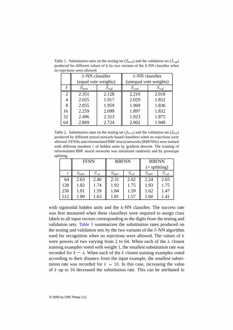
Table 1. Substitution rates on the testing set (Stest) and the validation set (Sval)produced for different values ofk by two variants of thek-NN classifier whenno rejections were allowed.
Table 2. Substitution rates on the testing set (Stest) and the validation set (Sval)produced by different neural-network-based classifiers when no rejections wereallowed. FFNNs and reformulated RBF neural networks (RBFNNs) were trainedwith different numbersc of hidden units by gradient descent. The training ofreformulated RBF neural networks was initialized randomly and by prototypesplitting.
with sigmoidal hidden units and thek-NN classifier. The success ratewas first measured when these classifiers were required to assign classlabels to all input vectors corresponding to the digits from the testing andvalidation sets. Table 1 summarizes the substitution rates produced onthe testing and validation sets by the two variants of thek-NN algorithmused for recognition when no rejections were allowed. The values ofkwere powers of two varying from 2 to 64. When each of thek closesttraining examples voted with weight 1, the smallest substitution rate wasrecorded fork = 4. When each of thek closest training examples votedaccording to their distance from the input example, the smallest substi-tution rate was recorded fork = 16. In this case, increasing the valueof k up to 16 decreased the substitution rate. This can be attributed to
the fact that the votes of allk training examples were weighted with val-ues that decreased from1 to 1=k, which reduced the contribution of themost distant among thek training examples. This weighting strategy im-proved the performance of thek-NN classifier, as indicated byTable 1.When no rejections were allowed, the performance of both variants ofthek-NN classifier was inferior to that of the neural networks tested inthese experiments. This is clearly indicated byTable 2, which summa-rizes the substitution rates produced on the testing and validation sets byFFNNs and reformulated RBF neural networks. The number of hiddenunits varied in these experiments from 64 to 512. The sets of prototypesused for initializing the supervised training of reformulated RBF neuralnetworks were produced by a random number generator and by the pro-totype splitting procedure outlined in Section 6. The performance of thetrained FFNNs on both testing and validation sets improved consistentlyas the number of hidden units increased from 64 to 256 but degradedwhen the number of hidden units increased from 256 to 512. In contrast,the performance of reformulated RBF neural networks on both testingand validation sets improved consistently as the number of radial basisfunction units increased fromc = 64 to c = 512. Both reformulatedRBF neural networks trained withc = 512 radial basis functions out-performed the best FFNN. Moreover, the performance of the best FFNNwas inferior to that of the reformulated RBF neural network trained withc = 256 radial basis functions using the initialization scheme employingprototype splitting. The best overall performance among all classifiersevaluated in this set of experiments was achieved by the reformulatedRBF neural network trained withc = 512 radial basis functions by gra-dient descent initialized by prototype splitting.
The success rate of thek-NN classifier and the neural-network-basedclassifiers was also measured when these classifiers were allowed to re-ject some ambiguous digits in order to improve their reliability. Thek-NN classifier was implemented in these experiments by assigning votesequal to 1 to thek closest training examples. This variant of thek-NNclassifier does not reject any digit ifk = 1. The percentage of digits re-jected by this variant of thek-NN classifier increases as the value ofkincreases. The rejection of digits by the FFNN and reformulated RBFneural networks was based on the strategy outlined above. According tothis strategy, the percentage of the rejected digits increases as the rejec-
reformulated RBF initialized randomlyreformulated RBF initialized by prototype splitting
(a)
0
0.5
1
1.5
2
0 2 4 6 8 10
% S
ubst
itutio
n
% Rejection
k-NNFFNN
reformulated RBF initialized randomlyreformulated RBF initialized by prototype splitting
(b)
Figure 10. Performance of thek-NN classifier, a feed-forward neural networkand two reformulated RBF neural networks tested on the NIST digits. The sub-stitution rate is plotted versus the rejection rate (a) on the testing set, and (b) onthe validation set.
tion parameterr increases above 0. Forr = 0, no digits are rejected andclassification is based on a winner-takes-all strategy. Figure 10 plots thepercentage of digits from the testing and validation sets substituted at dif-ferent rejection rates by thek-NN classifier, an FFNN with 256 hiddenunits, and two reformulated RBF neural networks with 256 radial basisfunctions. Both RBF neural networks were trained by the sequential gra-dient descent algorithm presented in Section 6. The supervised learningprocess was initialized in one case by randomly generating the initial setof prototypes and in the other case by determining the initial set of proto-types using prototype splitting. The training of all neural networks testedwas terminated based on their performance on the testing set. When norejections were allowed, all neural networks tested in these experimentsperformed better than various classification schemes tested on the samedata set [10], none of which exceeded the recognition rate of 97.5%. Inthis case, all neural networks outperformed thek-NN classifier, whichclassified correctly 97.79% of the digits from the testing set and 97.98%of the digits from the validation set. When no rejections were allowed,the best performance was achieved by the reformulated RBF neural net-work whose training was initialized by the prototype splitting procedureoutlined in Section 6. This network classified correctly 98.38% of thedigits from the testing set and 98.53% of the digits from the validationset. According to Figure10, thepercentageof digits from thetesting andvalidation sets substituted by all classifiers tested in these experimentsdecreased as the rejection rate increased. This experimental outcome ver-ifies that the strategy employed for rejecting ambiguous digits based onthe outputs of the trained neural networks is a simple and effective wayof dealing with uncertainty. Regardless of the rejection rate, all three neu-ral networks tested in these experiments outperformed thek-NN classi-fier, which substituted the largest percentage of digits from both testingand validation sets. The performance of the reformulated RBF neuralnetwork whose training was initialized by randomly generating the pro-totypes was close to that of the FFNN. In fact, the FFNN performedbetter at low rejection rates while this reformulated RBF neural networkoutperformed the FFNN at high rejection rates. The reformulated RBFneural network initialized by the prototype splitting procedure outlinedin Section 6 performed consistently better on the testing and validationsets than the FFNN. The same RBF network outperformed the reformu-lated RBF neural network initialized randomly on the testing set and on
the validation set for low rejection rates. However, the two reformulatedRBF neural networks achieved the same digit recognition rates on thevalidation set as the rejection rate increased. Among the three networkstested, the best overall performance was achieved by the reformulatedRBF neural network whose training was initialized using prototype split-ting.
9 Conclusions
This chapter presented an axiomatic approach for reformulating RBFneural networks trained by gradient descent. According to this approach,the development of admissible RBF models reduces to the selection ofadmissible generator functions that determine the form and properties ofthe radial basis functions. The reformulated RBF neural networks gen-erated by linear and exponential generator functions can be trained bygradient descent and perform considerably better than conventional RBFneural networks. The criteria proposed for selecting generator functionsindicated that linear generator functions have certain advantages over ex-ponential generator functions, especially when reformulated RBF neuralnetworks are trained by gradient descent. Given that exponential gener-ator functions lead to Gaussian radial basis functions, the comparison oflinear and exponential generator functions indicated that Gaussian radialbasis functions are not the only, and perhaps not the best, choice for con-structing RBF neural models. Reformulated RBF neural networks wereoriginally constructed using linear functions of the formg0(x) = x+ 2,which lead to a family of radial basis functions that includes inverse mul-tiquadratic radial basis functions [13], [20], [21]. Subsequent studies, in-cluding that presented in the chapter, indicated that linear functions of theform g0(x) = 1+ Æ x facilitate the training and improve the performanceof reformulated RBF neural networks [17].
The experimental evaluation of reformulated RBF neural networks pre-sented in this chapter showed that the association of RBF neural net-works with erratic behavior and poor performance is unfair to this pow-erful neural architecture. The experimental results also indicated that thedisadvantages often associated with RBF neural networks can only beattributed to the learning schemes used for their training and not to the
models themselves. If the learning scheme used to train RBF neural net-works decouples the determination of the prototypes and the updates ofthe output weights, then the prototypes are simply determined to satisfythe optimization criterion behind the unsupervised algorithm employed.Nevertheless, the satisfaction of this criterion does not necessarily guar-antee that the partition of the input space by the prototypes facilitates theimplementation of the desired input-output mapping. The simple reasonfor this is that the training set does not participate in the formation ofthe prototypes. In contrast, the update of the prototypes during the learn-ing process produces a partition of the input space that is specificallydesigned to facilitate the input-output mapping. In effect, this partitionleads to trained reformulated RBF neural networks that are strong com-petitors to other popular neural models, including feed-forward neuralnetworks with sigmoidal hidden units.
The results of the experiments on the NIST digits verified that refor-mulated RBF neural networks trained by gradient descent are strongcompetitors to classical classification techniques, such as thek-NN, andalternative neural models, such as FFNNs. The digit recognition ratesachieved by reformulated RBF neural networks were consistently higherthan those of feed-forward neural networks. The classification accuracyof reformulated RBF neural networks was also found to be superior tothat of thek-NN classifier. In fact, thek-NN classifier was outperformedby all neural networks tested in these experiments. Moreover, thek-NNclassifier was computationally more demanding than all the trained neu-ral networks, which classified examples much faster than thek-NN clas-sifier. The time required by thek-NN to classify an example increasedwith the problem size (number of examples in the training set), whichhad absolutely no effect on the classification of digits by the trained neu-ral networks. The experiments on the NIST digits also indicated that thereliability and classification accuracy of trained neural networks can beimproved by a recall strategy that allows the rejection of some ambiguousdigits.
The experiments indicated that the performance of reformulated RBFneural networks improves when their supervised training by gradient de-scent is initialized by using an effective unsupervised procedure to deter-mine the initial set of prototypes from the input vectors included in the
training set. An alternative to employing the variation of thec-means al-gorithm employed in these experiments would be the use of unsupervisedalgorithms that are not significantly affected by their initialization. Thesearch for such codebook design techniques led to soft clustering [2],[11], [14], [18], [19] and soft learning vector quantization algorithms[12], [15], [16], [18], [19], [24], [27], [35], [41]. Unlike crisp cluster-ing and vector quantization techniques, these algorithms form the pro-totypes on the basis ofsoft instead of crisp decisions. As a result, thisstrategy reduces significantly the effect of the initial set of prototypeson the partition of the input vectors produced by such algorithms. Theuse of soft clustering and LVQ algorithms for initializing the training ofreformulated RBF neural networks is a particularly promising approachcurrently under investigation. Such an initialization approach is stronglysupported by recent developments in unsupervised competitive learning,which indicated that the same generator functions used for constructingreformulated RBF neural networks can also be used to generate soft LVQand clustering algorithms [19], [20], [22].
The generator function can be seen as the concept that establishes a directrelationship between reformulated RBF models and soft LVQ algorithms[20]. This relationship makes reformulated RBF models potential targetsof the search for architectures inherently capable of merging neural mod-eling with fuzzy-theoretic concepts, a problem that attracted considerableattention recently [39]. In this context, a problem worth investigating isthe ability of reformulated RBF neural networks to detect the presenceof uncertainty in the training set and quantify the existing uncertainty byapproximating any membership profile arbitrarily well from sample data.
References
[1] Behnke, S. and Karayiannis, N.B. (1998), “Competitive neural treesfor pattern classification,”IEEE Transactions on Neural Networks,vol. 9, no. 6, pp. 1352-1369.
[2] Bezdek, J.C. (1981),Pattern Recognition with Fuzzy ObjectiveFunction Algorithms,Plenum, New York, NY.
[3] Broomhead, D.S. and Lowe, D. (1988), “Multivariable functional
interpolation and adaptive networks,”Complex Systems, vol. 2, pp.321-355.
[4] Cha, I. and Kassam, S.A. (1995), “Interference cancellation usingradial basis function networks,”Signal Processing,vol. 47, pp. 247-268.
[5] Chen, S., Cowan, C.F.N., and Grant, P.M. (1991), “Orthogonalleast squares learning algorithm for radial basis function networks,”IEEE Transactions on Neural Networks,vol. 2, no. 2, pp. 302-309.
[6] Chen, S., Gibson, G.J., Cowan, C.F.N., and Grant, P.M. (1991),“Reconstruction of binary signals using an adaptive radial-basis-function equalizer,”Signal Processing,vol. 22, pp. 77-93.
[7] Cybenko, G. (1989), “Approximation by superpositions of a sig-moidal function,”Mathematics of Control, Signals, and Systems,vol. 2, pp. 303-314.
[8] Gersho, A. and Gray, R.M. (1992),Vector Quantization and SignalCompression,Kluwer Academic, Boston, MA.
[10] Grother, P.J. and Candela, G.T. (1993), “Comparison of handprinteddigit classifiers,”Technical Report NISTIR 5209, National Instituteof Standards and Technology, Gaithersburg, MD.
[11] Karayiannis, N.B. (1996), “Generalized fuzzyc-means algorithms,”Proceedings of Fifth International Conference on Fuzzy Systems,New Orleans, LA, pp. 1036-1042.
[12] Karayiannis, N.B. (1997), “Entropy constrained learning vectorquantization algorithms and their application in image compres-sion,” SPIE Proceedings vol. 3030: Applications of Artificial Neu-ral Networks in Image Processing II, San Jose, CA, pp. 2-13.
[13] Karayiannis, N.B. (1997), “Gradient descent learning of radial basisneural networks,”Proceedings of 1997 IEEE International Confer-ence on Neural Networks, Houston, TX, pp. 1815-1820.
clustering,”IEEE Transactions on Fuzzy Systems, vol. 5, no. 4, pp.622-628.
[24] Karayiannis, N.B., Bezdek, J.C., Pal, N.R., Hathaway, R.J., and Pai,P.-I (1996), “Repairs to GLVQ: A new family of competitive learn-ing schemes,”IEEE Transactions on Neural Networks,vol. 7, no.5, pp. 1062-1071.
[25] Karayiannis, N.B. and Mi, W. (1997), “Growing radial basis neuralnetworks: Merging supervised and unsupervised learning with net-work growth techniques,”IEEE Transactions on Neural Networks,vol. 8, no. 6, pp. 1492-1506.
[26] Karayiannis, N.B. and Pai, P.-I (1995), “Fuzzy vector quantiza-tion algorithms and their application in image compression,”IEEETransactions on Image Processing, vol. 4, no. 9, pp. 1193-1201.
[27] Karayiannis, N.B. and Pai, P.-I (1996), “Fuzzy algorithms for learn-ing vector quantization,”IEEE Transactions on Neural Networks,vol. 7, no. 5, pp. 1196-1211.
[29] Kohonen, T. (1989),Self-Organization and Associative Memory,3rd Edition, Springer-Verlag, Berlin.
[30] Kohonen, T. (1990), “The self-organizing map,”Proceeding of theIEEE, vol. 78, no. 9, pp. 1464-1480.
[31] Linde, Y., Buzo, A., and Gray, R.M. (1980), “An algorithm for vec-tor quantization design,”IEEE Transactions on Communications,vol. 28, no. 1, pp. 84-95.
[32] Lippmann, R.P. (1989), “Pattern classification using neural net-works,” IEEE Communications Magazine, vol. 27, pp. 47-54.
[33] Micchelli, C.A. (1986), “Interpolation of scattered data: Distancematrices and conditionally positive definite functions,”Construc-tive Approximation, vol. 2, pp. 11-22.
[34] Moody, J.E. and Darken, C.J. (1989), “Fast learning in networksof locally-tuned processing units,”Neural Computation, vol. 1, pp.281-294.
[35] Pal, N.R., Bezdek, J.C., and Tsao, E.C.-K. (1993), “Generalizedclustering networks and Kohonen’s self-organizing scheme,”IEEETransactions on Neural Networks, vol. 4, no. 4, pp. 549-557.
[36] Park, J. and Sandberg, I.W. (1991), “Universal approximation us-ing radial-basis-function networks,”Neural Computation, vol. 3,pp. 246-257.
[37] Park, J. and Sandberg, I.W. (1993), “Approximation and radial-basis-function networks,”Neural Computation, vol. 5, pp. 305-316.
[38] Poggio, T. and Girosi, F. (1990), “Regularization algorithms forlearning that are equivalent to multilayer networks,”Science, vol.247, pp. 978-982.
[39] Purushothaman, G. and Karayiannis, N.B. (1997), “Quantum Neu-ral Networks (QNNs): Inherently fuzzy feedforward neural net-works,” IEEE Transactions on Neural Networks, vol. 8, no. 3, pp.679-693.
[40] Roy, A., Govil, S., and Miranda, R. (1997), “A neural-networklearning theory and a polynomial time RBF algorithm,”IEEETransactions on Neural Networks,vol. 8, no. 6, pp. 1301-1313.
[41] Tsao, E.C.-K., Bezdek, J.C., and Pal, N.R. (1994), “Fuzzy Kohonenclustering networks,”Pattern Recognition, vol. 27, no. 5, pp. 757-764.
[42] Whitehead, B.A. and Choate, T.D. (1994), “Evolving space-fillingcurves to distribute radial basis functions over an input space,”IEEE Transactions on Neural Networks,vol. 5, no. 1, pp. 15-23.