New Regularization Algorithms for Solving the Deconvolution Problem in Well Test Data Interpretation*
Vladimir Vasin1, Georgy Skorik1, Evgeny Pimonov2, Fikri Kuchuk3 1Institute of Mathematics and Mechanics UrB RAS, Ekaterinburg, Russia
2Schlumberger Moscow Research, Moscow, Russia 3Schlumberger Riboud Product Center, Paris, France
E-mail: [email protected] Received June 29, 2010; revised September 17, 2010; accepted September 20, 2010
Abstract Two new regularization algorithms for solving the first-kind Volterra integral equation, which describes the pressure-rate deconvolution problem in well test data interpretation, are developed in this paper. The main features of the problem are the strong nonuniform scale of the solution and large errors (up to 15%) in the input data. In both algorithms, the solution is represented as decomposition on special basic functions, which satisfy given a priori information on solution, and this idea allow us significantly to improve the quality of approximate solution and simplify solving the minimization problem. The theoretical details of the algo-rithms, as well as the results of numerical experiments for proving robustness of the algorithms, are pre-sented. Keywords: Deconvolution Problem, Volterra Equations, Well Test, Regularization Algorithm,
Quasi-Solutions Method, Tikhonov Regularization, A Priori Information, Discrete Approximation, Non-Quadratic Stabilizing Functional, Special Basis
1. Introduction The pressure-rate deconvolution problem transpires for model-identification processes in pressure-transient well test data interpretation for solving the first-kind Volterra integral equation of convolution type [1] that is given as
,0),(=)()(0
TttpdgtqAgt
(1)
].[0,][0,: 22 TLTLA
This equation is a consequence of Duhamel’s super-position principle, which holds for a wellbore/reservoir system at certain conditions, namely, when the system is considered as a linear one. The principle states that the measured pressure drop )(=)( 0 tpptp is a convolu-tion of the measured flow rate )(tq and reservoir re-sponse function ,)(tg which is a time-derivative of the constant-unit-rate pressure solution .)/(=)( dttdptg u
Here,
0p is the initial reservoir pressure (pressure in undisturbed reservoir), )(tp is pressure measured in the
wellbore, in particular, on the surface or at bottomhole, and T is the total duration of the well test. Functions
)(tg and )(tpu are unknown and needed to be esti-
mated by a deconvolution algorithm as an inverse prob-lem.
Functions, ( )up t , ( )g t , and such as ( ) = ( ) / lnutg t dp t d t contain important information about
the wellbore/reservoir system. Normally, they are plotted as a function of time as semilog or log-log graphs [2]. For instance, an initial part of a log-log plot of )(tpu
versus time yields the wellbore storage coefficient. Res-ervoir permeability and wellbore skin damage can be calculated from a log-log plot of )(ttg versus time or a semilog plot of )(tpu
during the middle time period. Identification of certain geological features such as faults, fractures, reservoir boundaries, etc., is possible from middle and late time periods.
Peculiarities of the deconvolution problem in well test interpretation are in the following:
1) real input data can be discontinuous and oscillating (see data 2);
2) a solution )(tg is rather multi-scale (see data 1); 3) these specific features of the problem cause serious
*The work has been supported by Schlumberger, and partially supportedby Russian Foundation for Basic Research, project 09–01–00053.
difficulties for reconstruction of a desired solution and its interpretation.
As is well known [3], reservoir response )(tg (the solution of the diffusivity equation) satisfies the follow-ing a priori given constraints:
( 1) ( ) / 0, = 0,1,2,k k kd g t dt k (2)
It is worth noting that during development of the algo-rithms using a priori constraints (2), one usually employs not more than three following conditions [4]:
( ) = : 0 ( ) , ( ) 0, ( ) 0g t Q g g t c g t g t (3)
Let us briefly review a few methods presented in the petroleum literature for solving a pressure-rate deconvo-lution problem in linear setting (1). Linear programming methods containing a priori constraints (3) were devel-oped by Coats et al. [3] and Gajdica et al. [5]. Different rules for discretization of the convolution integral with different modifications, which resulted in explicit recur-sive formulas, were proposed in a number of works. Hutchinson and Sikora [6] used a trial and error proce-dure with correcting multipliers, Katz et al. [7] used a linear recursive formula and tried considering a priori information (3), Jargon and van Poollen [8] added loga-rithmic interpolation to a recursive formula, Thompson and Reynolds [9] proposed three methods based on dif-ferent discretization rules, Bostic et al. [10] and Kuchuk [11] simply used pure recursive formulas without any modifications. In the work by Kucuk and Ayestaran [12] two methodologies for deconvolution were proposed, namely, Laplace transform deconvolution and curve-fit approximations. A linear least-squares approach with a priori constraints (3) was proposed by Kuchuk et al. [4]. Baygun et al. [13] also used the linear least-squares me-thod with a special type of inequalities called the nor-malized autocorrelation constraints. Spectral methods, based on a convolution theorem, which in the case of Equation (1) holds approximately for both Laplace and Fourier transforms, were developed by Roumboutsos and Stewart [14], Mendes et al. [15], Bourgeois and Horne [16], Onur and Reynolds [17].
Unfortunately, almost all methods using recursive formulas failed on pressure data with noise up to 1%. Linear programming methods and linear least-squares approaches worked insufficiently when errors in flow rate data were 1 to 2%. Spectral methods are the simplest, but they mostly failed with noisy data.
In the early 2000s, von Schroeter et al. [18,19] pre-sented a completely new methodology for the pressure- rate deconvolution inverse problem. First, they trans-formed the linear Equation (1) to a nonlinear one
)(=)()( )(ln
tpdeetqzA zt
(4)
by using the transformation
)).((ln=)(,ln= gz
This replacement makes the condition 0)( tg to hold automatically. Second, the total nonlinear least- squares method was used with the Tikhonov regulariza-tion in which a constraint was imposed on the curvature of the solution. This methodology not only estimates the solution )(tg but also allows for correcting the flow rates )(tq and the initial reservoir pressure
0p if they contain large errors. But Levitan [20] showed that the pressure-rate deconvolution algorithm fails when incon-sistent input data are used. He proposed a modified methodology. In a subsequent paper by Levitan et al. [21], valuable suggestions were made for practical appli-cations of the pressure-rate deconvolution. Pimonov et al. [22,23] further modified the deconvolution algorithm of von Schroeter et al. [18,19] and Levitan [20]. The modi-fication was done by introducing a more general objec-tive function in the Levenberg-Marquardt minimization procedure. This algorithm was successfully applied by Pimonov et al. [22,23] to deconvolution of drillstem test data and wireline formation tester data. Recently, a to-tally different approach for solving the nonlinear Equa-tion (1) was proposed by Ageev et al. [24], where the authors used an iteratively regularized modified Leven-berg-Marquardt method.
In parallel to von Schroeter et al. [18,19] and Levitan [20] methodologies, research has been continued to solve the linear convolution integral equation (1) directly. For instance, a projection method based on B-splines repre-sentation of the solution was proposed by Ilk et al. [25]. The method appears to be quite robust, although it does not take into account errors in flow rates and the initial reservoir pressure. Andrecut and Madni [26] and Andre-cut [27] studied three methods: 1) Tikhonov regulariza-tion, 2) Krylov subspace projection method, and 3) sto-chastic Monte-Carlo. The authors stated that the stochas-tic Monte-Carlo method was more robust than the other two. Overall disadvantages of these three methods come from the fact that flow rate errors are not accounted for.
Finally, Cinar et al. [28] compared efficiency and ro-bustness of pressure-rate deconvolution algorithms of von Schroeter et al. [18,19], Levitan [20], and Ilk et al. [25]. First, they stated that the regularization approach used by Ilk et al. [25] seems to be weaker; hence, this makes the algorithm less tolerant to the errors in pressure and rate data compared to the von Schroeter et al. [18], [19] and Levitan [20] algorithms. Second, these last two algorithms have certain efficiency and robustness.
This work is a continuation of a study done by Vasin et al. [29,30]. We now propose two algorithms for solv-ing the linear convolution integral Equation (1) and pre-
sent a theoretical analysis of the algorithms for pressure- rate deconvolution.
The first algorithm proposed is based on a quasi-solu-tions method, i.e., an initial problem (1) is reduced to a minimization problem
2
2min :
LAg p g Q
on a compact set Q (see (6)), which is a closure of the set Q .
It is very important that a solution of the minimization problem is found as an expansion by a special basis, which elements satisfy a priori constraints.
It is worth noting that an attempt to develop a decon-volution algorithm based on discrepancy minimization has been done by Kuchuk et al. [4]. However, an unsuit-able minimization procedure was used, and it led to un-stable deconvolved results. The minimization algorithm proposed in our work appears to be more effective. At the same time, the problem with an initial approximation for the solution is successfully resolved. Due to using a special basis, we have possibility to choose always
0=)(tg as an initial point (guess) for iterative algo-rithms used in the numerical minimization. Usually spe-cial procedures are required to find an appropriate start-ing point for iterative processes of minimization (see papers mentioned above).
The second algorithm uses the Tikhonov regulariza-tion method with constraints (3), i.e., an approximate solution is calculated by regularized conditional minimi-zation
2
2min [ ] :
LAg p g g Q (5)
where a stabilizing functional is nonlinear (non- quadratic), which is opposite to traditional scheme (see [31]). This feature of the functional significantly improves quality of an approximate solution. The func-tional is defined explicitly further in Section 4, contained detailed description of the second algorithm. To decon-volve data with a large measurement errors in flow rates
,)(tq a modified version of the algorithm is also devel-oped. In the modification, flow rates at the estimated solution )(tg are additionally corrected using quadratic Tikhonov regularization.
Our paper is organized as follows: investigation of the algorithm based on the quasi-solutions method is given in Section 2; stability of discrete approximations based on collocation method is proven in Section 3; Section 4 is devoted to the study of the Tikhonov regularization algo-rithm; Section 5 presents the details of the scheme for flow rates )(tq correction; synthetic well test examples are presented in Section 6 to illustrate the methodology.
2. Quasi-Solutions Method and Its Features Before studying the quasi-solutions method, several as-sumptions are made on the input data. Let ( )q t be a continuous function and (0) 0.q Let us assume that an integral operator A in (1) acts from ][0,2 TL into
.][0,2 TL On this pair of spaces (as well as on the spaces of continuous functions), operator A is a compact one (completely continuous). Thus, A does not have a con-tinuous inverse operator ,1A so the problem is essen-tially ill-posed and the solution is strongly sensitive to errors in the input data.
Further, we will consider the set Q of a priori con-straints, which is wider than the initial set ,Q namely,
)(,)(0:][0,{= 2 tgCtgTLgQ
function},convexincreasing-nona is (6)
i.e., differentiability of )(tg is not assumed. The set Q is a compact set in ][0,2 TL (in contrast to the set ,Q which is nonclosed), so a basis with non-smooth (e.g., piecewise linear) functions could be used.
Real data ( )q t and ( )p t of problem (1) have meas-urement errors, so it is assumed that instead of exact in-put data ,)(tq ,)(tp we have approximate input data
)(tq and )(tp with the following estimations of measurement errors:
2 2, .
L Lq q p p (7)
Equation (1) might not have a solution for a given right-hand-side ][0,2 TLp because the actual range of A is nonclosed. Thus, in a general case under the solution of problem (1), we will understand that it is a quasi-solution (see [32], p. 36); i.e., a function ˆ,g which realizes minimum of discrepancy:
2 2
2 2ˆmin : = ,
L LAg p g Q Ag p (8)
on a compact set Q (see lemma 2.2). Equation (8) is solvable for any function ][0,2 TLp because the set Q is a compact and the operator A is continuous.
Solvability conditions for (1) and (8) are given in the following lemma.
Lemma 1: Let ( ),q t ( )p t be continuously differ-entiable functions, and (0) 0.q Then Equations (1) and (8) are uniquely solvable.
Proof. By differentiating both parts of Equation (1), we obtain the Volterra equation of the second kind
0
(0) ( ) ( ) ( ) = ( ),t
q g t q t g d p t (9)
which has a unique solution due to generalized principle of contracting mappings [33]. As long as any solution of Equation (1) is a solution of Equation (9), then (1) cannot
have several solutions; therefore, ( ) 0Ker A . Since an objective functional of (8) is strictly convex at these conditions, a quasi-solution is also unique.
Further, only the case for {0}=)(ker A is considered. The general situation is discussed at the end of the sec-tion (see Theorem 2.2).
Lemma 2: The set ,Q defined by relation (6), is a compact in 2[0, ].L T
Proof is similar to one for the set Q of monotone functions (see [34]).
Let us consider problem (8) with approximate data that satisfy relations (7):
2
2min : ,
LA g p g Q (10)
where
0( ) = ( ) ( ) .
TA g t q t g d
Denote the solution of problem (10) as .ˆ ,g Theorem 1: Let ,{0}=)(ker A ,{0}=)(ker A and
the approximation conditions (7) hold. Then problem (10) is uniquely solvable and the following convergence holds:
2
,2, 0
ˆ ˆ = 0,limL
g g
(11)
where g is the solution of problem (8). In general case, when ,)(ker A )(ker A are not triv-
ial sets, the problems (8), (10) are non-uniquely solvable. Then the following theorem holds.
Theorem 2: Let problems (8) and (10) be non- uniquely solvable and ,G
,G be the sets of their cor-responding solutions.
Then,
,ˆ, 0 ˆˆ ˆ , ,
ˆ ˆ = 0.suplim infg G g G
g g
The proofs of Therorems 2.1, 2.2 can be obtain on the basis of the general theorem on the quasi-solution me-thod for operator equations [32].
Thus, quasi-solutions are stable with respect to errors in the input data and }ˆ{ ,g generates a regularized family of approximate solutions. In turn, the quasi-solu-tions method generates a regularizing algorithm [31]. 3. Stability of Discrete Approximations 3.1. Construction and Study of a Basis For a discrete approximation of the equation
0
( ) ( ) = ( ), 0 ,t
A g q t g d p t t T (12)
a collocation method is used. Let )(thnj
be some basis in .][0,2 TL In this case, integral Equation (12) can be approximated by a system of algebraic linear equations
),(=)()(=)(0
in
i
it
in
n tpdgtqgA (13)
1, 2, , ,i n
where ,)(=)(1
1=thctg n
jnj
n
j
n ,](0,Tti it are colloca-
tion points (time points of pressure )(tp measurements in the well), ,G: 1 nn
n RA 1G n is a finite-dimen- sional subspace in ,][0,2 TL which is generated by
1n elements of the basis, and nR is n-dimensional Euclidean space with the norm
,=2
1=
2
ii
n
ipp ,= 1 iii tt ( 0=0t ).
The basic functions are built with connection to the grid ,}{ 0=
nj
nj ,0=0
n ,= Tnn on which the solution is
searched by the following rule:
.1,for 0
,for 1
,1for 1
)(
nj
nj
h
nj
njn
j
nj
It is obvious that )(njh are non-negative, non-increa-
sing, and convex functions; i.e., they satisfy the same a priori constraints as the desired solution. This property of the basis is very important, since allows us to get a stable approximation of the desired solution for Equation (1) with real well tests.
Theorem 3: Let
0.=maxlim 11
nj
nj
njn
(14)
Then the system of functions }{ njh is independent
and for any function ][0,2 TLg , there exists a se-quence of vectors ),,,(= 121
nn
nnn cccc such that
0;=)()(lim
21
1=0
dhcg nj
nj
n
j
T
n
and for any function ,g Q the coefficients { }njc are
non-negative. Proof. Let the first assumption be that )(tg is a con-
tinuous function defined at .][0,T The coefficients njc
are calculated consecutively from the relations
.,0,1,=),(=)(1
1=
nihcg inj
nj
n
j
ni
(15)
Assuming ni = in (15), we have 1 = ( ) = ( );n nn nc g g T
then we define the function 1 1( ) = ( ) .nng g c Inserting
1= ni in (15), we obtain 1 1 1( ) = ( ),n n n n nn n n n ng c c h
which gives 1 1 1= ( ) / ( );n n n nn n n nc g h then we define the
For ,k we have a formula for calculation of the coef-ficients
1 1= ( ) / ( ),n n n nn k k n k n k n kc g h (16)
where the functions )(kg are calculated by recurrent relations
1 1 1( ) = ( ) ( ).n nk k n k n kg g c h (17)
Let ;Qg i.e., it be non-negative, non-decreasing, and convex at ][0,T function; therefore, it is a conti- nuous function. Non-negativity of the coefficients n
ic follows both from Formula (16) and from the fact that the function )(kg defined by relation (17) has the same properties within the segment ][0, 1knt as does the function )(g .
Now, let 2[0, ].g L T Since the set of continuous functions is a dense one in ,][0,2 TL there exists a con-tinuous function g such that
[0, ]2.
L Tg g Fol-
lowing the algorithm described previously, let { ( )}ng be built using the function ( ).g Therefore, due to condition (14), { ( )}ng is pointwise converging to ,g which implies convergence in .][0,2 tL
It follows from an obvious inequality ngggggg that the family of the func-
tions { ( )}njh generates the basis in 2[0, ].L t
3.2. Convergence of Discrete Approximations To complete the investigation of discretization for prob-lem (10), we approximate the set of a priori constraints Q by a sequence of the sets
,0),(=)(:G=1
1=
1
nj
nj
nj
n
j
nnnn cthctggQ
where in the representation of ,ng the coefficients njc
are calculated by the algorithm from theorem 3. A dis-crete analogue of the minimization problem (10) has the form
2min : ,n n n n nA g p g Q (18)
where the mapping nA is defined by Formula (13),
1 2= ( ( ), ( ), , ( )).n np p t p t p t Theorem 4. Let )(tq be a continuous function and
the problem (10) be uniquely solvable. Then problem (18) has a solution ,ˆng which strongly converges to the so-lution of (10) in the space ][0,2 TL as .n
Proof. Based on the work by Vasin [35] it is sufficient to check the following conditions:
1) AAn (discrete convergence of the operators); 2) AAn (discrete weak convergence of the
operators); 3) ppn (discrete convergence of the ele-
ments); 4) for any function ,Qg there exists such
n ng Q that 2
= 0;lim n Ln
g g
5) discrete weak convergence ,nkg g ,n nk k
g Q implies .g Q
A definition of discrete convergence could be found in Stummel [36], Grigorieff [37], Vainikko [38] (see also [35,39]).
The properties (1–3) are established in the same way as for the case of the integral Fredholm operator (see [39]). Since ,ih Q it holds nQ Q . Therefore, the property (4) follows from completeness of the system
}{ njh (completeness was established in theorem 3.1). If ,
knkn Qg ,weakly gg then due to Lyusternik and Sobolev [40], p. 216, one can find a sequence of
convex combinations ikni
N
iN gg 1== (
=1= 1,
N
ii
0i ), which strongly converges to .g Because
nQ Q and Q is a convex closed set, then .g Q
Reference to the work by Vasin [35] completes the proof of the theorem.
It is easy to see that problem (18) is equivalent to the problem
2min : 0 ,n
n n ic p c nA (19)
where
1 1= ( ( ), ( ), , ( )),n np p t p t p t
1 2 1= ( , , , ),n n nn nc c c c
and the components of the matrix nA have the follow-
ing structure:
0
( ) = ( ) ( ) .ti
nij i jq t h d nA
Problem (19) is resolved by the conditional gradient method (see [41]). 4. Tikhonov Regularization Method with
Non-Linear Stabilizer 4.1. Convergence of Regularized Solutions Numerical processing synthetic data with relatively large errors in flow rates ( )q t and pressures ( )p t have shown that the quasi-solutions method did not give a smooth solution, which would be appropriate for inter-pretation. Therefore, it is necessary to add regularization by a non-linear (non-quadratic) stabilizer and a pri-ori constraints:
i.e., in contrast to the set ,Q we additionally introduced the constraint from below on the function .)(tg From solution of the initial problem (1) it is seen that this con-straint could be considered as true and we do not lose generality.
Further, we explain the reasons for the current type of the stabilizer .][g It is well known [18,19] that at transition from a linear Equation (1) to a nonlinear state-ment (4), the replacements of the variable ln= and the function ))((ln=)( gz are used. Now, if in a nonlinear deconvolution statement the stabilizing func-tional is taken in the form
dzzT
a
2ln
ln
)]([=][
and an inverse replacement is done, then the functional
)()/()()/([=][ 1/23/2 tgggggT
a
dgg 223/2 ]))()/((
is obtained. Eliminating less significant terms with the first derivative, we obtain stabilizer (21).
It is worth noting that using a traditional norm in So-bolev space ][0,2
2 TW instead of ][g is not effective. Numerical experiments shown that the stabilizer
][g takes into account more better multi-scale nature of the desired solution .)(tg
Theorem 5: Let problem (1) have a unique solution .
~],[ˆ 2
2 QTaWg If for approximate data ,q ,)(tp approximation conditions (7) hold, then for 0> problem (20) is solvable, possibly in a non-unique way. And if ,0),( 0),(/)( 2 as ,0, then extreme functions )(),( tg converge to the solu-tion g in the space ;],[1 TaC i.e.,
,)(ˆ)(sup ),( tgtgTta
( , ) ˆ( ) ( )0, , 0.
dg t dg t
dt dt
(23)
Proof. Let us denote as ][g the objective func-tional of problem (20). Let
ng be a minimizing se-quence; i.e., ,][ dgn .n Then for ,0>
,][ cgn where c is constant, i.e. ][ ng is a uni-
formly bounded sequence. Since Qgn
~ (see (22)), it holds Cgb n and, consequently,
,)(=)]()/([)]([ 2322
3
cgdggdgC
ann
T
a
n
T
a
and it follows that ],[22 TaWgn and .12
2cg
Wn Any closed bounded set from ],[2
2 TaW is a weakly compact one, so there exists a weakly converging sub-sequence .],[2
2 TaWggkn weakly Due to the em-
bedding theorems (see [42,43]), existing of such weakly converging subsequence implies uniform convergence
,],[),()(),()( Tattgtgtgtgknkn (24)
and .~Qg
Let us prove that the sequence )()/(=)( 3/2 tgtgttf
knknk weakly converges to )()/(3/2 tgtgt in .],[2 TaL This is a consequence of the
following relations:
3/2 3/2( ) / ( ) ( ) ( ) / ( ) ( )T T
n nk ka a
t g t g t v t dt t g t g t v t dt
3/2 3/21 1 ( )( ) ( ) ( ) ( ) .
( ) ( ) ( )
T T
n nk kna ak
v tg t t v t dt g t g t t dt
g t g t g t
The first term in the right-hand-side of the relation tends to zero due to both boundedness of weakly con-verging sequence and uniform convergence (24); the second term tends to zero due to weak convergence of
.)(tgkn
Taking into account continuity (and, consequently, weak continuity) of the operator A and weak semi- continuity from below the norm in the space ,2L we have
22 3/2
2( ) / ( )
T
La
d A g p t g t g t dt
2 23/2
2
( ) / ( ) = ,liminfT
n n nk k kLn a
A g p t g t g t dt d
i.e., the function )(tg realizes minimum of the objec-tive functional in (20).
Let us redefine the function )(tg as .)(tg For this function, the following inequalities hold:
Conditions of this theorem for the parameters imply boundedness
2),( ][ cg and, as a consequence (see
above), boundedness ( , ){ }g in the space .],[22 TaW
This means that one can find a subsequence ( , ) weaklyk kg g weakly converging in .],[2
2 TaW Considering weak half-continuity from below of the sta-bilizing functional ,][g we have bottom equation:
These relations mean that g~ is the solution of Equa-tion (1), and consequently, .ˆ=~ gg Since g is a unique weak limit point, it holds gg ˆweakly),( in
.],[22 TaW Using the theorem about compact imbedding
in ],[22 TaW and in ],[1 TaC [42,43], we obtain (23).
Remark. After discretization of problem (20) on the base of the scheme described in secton 3, the conjugate gradients method (see [41]) is used. 5. Correction of the Flow Rate Function At maximum errors in flow rates )(tq (up to 15%) and in pressures )(tp (up to 5%), strong distortions appear in the solution )(tg and )(tpu
obtained by the Tik-honov regularization algorithm, which makes interpre-tation of the solution on the log-log derivative plot al-most impossible. In this case, an additional correction of the function )(tq is suggested using the following procedure:
1) solve problem (20) for noisy ,q ,p and calcu-late ;)(tg
2) use the calculated )(tg in Equation (1), which is now considered as the equation with unknown function
)(tq
;=)()(0
pdtgqBqT
(25)
3) use the Tikhonov method (see [31]) for an ap-proximate calculation of )(tq from Equation (25) in the form
2 2
22 2
min : [0, ] ,L L
Bq p q q q L T (26)
where the regularization parameter is chosen from the relation
;: qqq
here q is a noisy flow rate, is its relative error lev-el, and q is the solution of (26);
4) resolve problem (20) using the calculated ;)(~ tq 5) repeat the steps (1–4) several times; the calculated )(tg is considered as an approximate solution of an ini-
tial problem (1). This procedure could be implemented also for the qu-
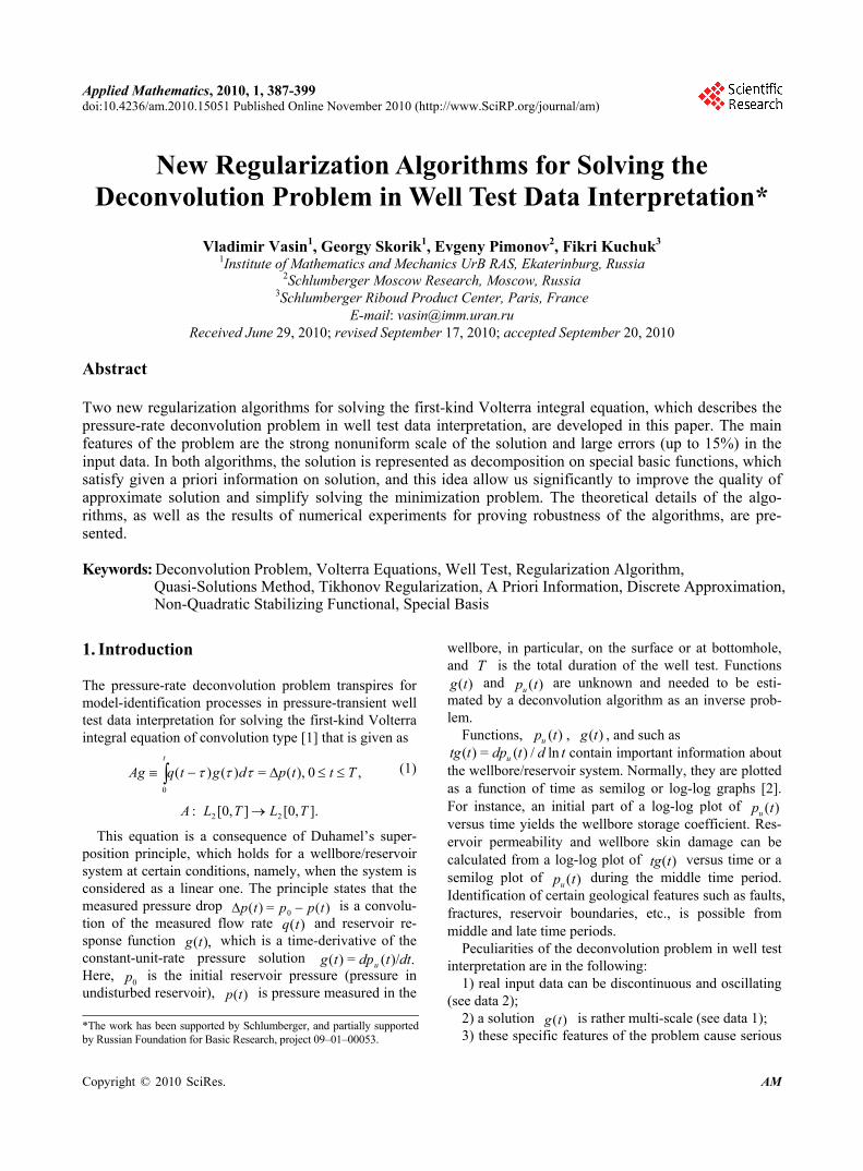
asi-solutions algorithm. Numerical experiments with the second algorithm (Tikhonov regularization) showed that after several iterations on g and ,q the function )(tq was corrected and the quality of the solution was im-proved. 6. Numerical Experiments The algorithms were tested on two synthetic data (see Figures 1 and 6), contained discrete functions )(tp and
,)(tq and were given on different grids with different levels of noise (errors). Exact solutions )(tpu
and ( ) / ln ( )udp t d t tg t in these cases are known and allow
for estimating quality of the solutions obtained by the algorithms. Results from testing the algorithms on two sets of synthetic data are presented below.
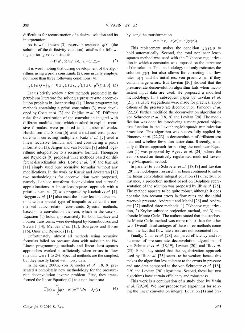
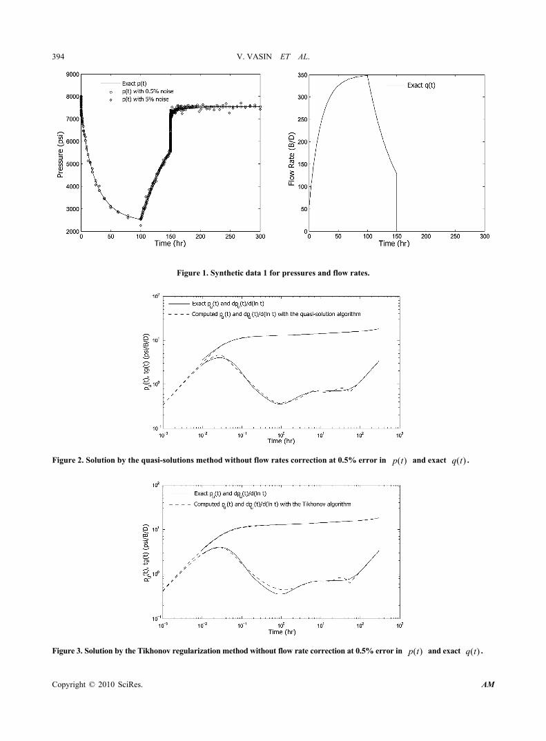
All calculations were carried out at the exact value of the initial reservoir pressure .0p Numerical experi-ments for the first synthetic data (Figure 1) were con-ducted for noisy )(tp with 0.5% and 5% errors and exact .)(tq For the second set of synthetic data (Figure 6), experiments were performed at noisy )(tp with a 1% error and exact ,)(tq as well as at )(tp with a 1% error and )(tq with a 15% error.
In Figures 2, 3, 4, and 5 results of calculations for synthetic data 1 (Figure 1) with pressure errors to 0.5% and 5% ( )(tq is exact) are presented on a log-log scale. Despite the fact that these data contain small amounts of information because 0=)(tq over a large part of the time period, the solution is reconstructed with appropri-ate accuracy.
Exact and numerical solutions for synthetic data 2 with 1% errors in pressure and exact )(tq as well as
Figure 10. Solution by the Tikhonov regularization without flow rate correction at 1% error in )(tp and 15% error in )(tq .
Figure 11. Solution by the Tikhonov regularization with flow rate correction at 1% error in )(tp and 15% error in )(tq .
The relative error of )(tg is 10.7% and 4.45% for ( )uq t .
with 1% errors in pressure and 15% maximum error in flow rates are shown in Figures 7, 8, 9 and 10. It is ob- vious that the solution is reconstructed with sufficient accuracy when there are no errors in flow rates; however, significant distortions are visible at 15% error in flow rates. It is necessary to correct flow rates according to the procedure described in Section 5. After 5 to 15 iterations of this correction, the quality of the solution is improved significantly (compare Figure 10 and Figure 11). It is worth noting that the Tikhonov method gives a more smooth solution for the calculations than with the quasi- solutions method, which makes easier interpretation. 7. Conclusions Two regularization methods for solving the deconvolu-tion problem are proposed and all stages of the algo-
rithms are theoretically established. The effectiveness of the methods is achieved by using all of the a priori in-formation about the solution, choosing the non-quadratic stabilizing functional, and using a special basis for ap-proximation of the solution.
Numerical experiments performed on synthetic data with error levels to 5% for pressures )(tp and to 15% for flow rates )(tq show effectiveness of the algorithms we have developed.
The advantage of the algorithms is that in iterative mi-nimization processes the initial approximation can be easily chosen, namely as a zero function. The quasi-so- lutions method allows for avoiding the cumbersome procedure for selecting regularization parameters. Moreover, the special basis for establishing approximate solutions makes an a priori constrain (6) to be true, and this property significantly improves the quality of ap-
proximate solution. It is worth noting that in our work, a theoretical foundation for all stages of the developed algorithms is performed, which contrasts works by others on the pressure-rate deconvolution problem, known to us and referenced in the literature. 8. References [1] A. F. van Everdingen and W. Hurst, “The Application of
the Laplace Transformation to Flow Problems in Reservoirs,” Transactions of American Institute of Min- ing, Metallurgical, and Petroleum Engineers, Vol. 186, 1949, pp. 305-324.
[2] D. Bourdet, J. A. Ayoub and Y. M. Pirard, “Use of Pressure Derivative in Well-Test Interpretation,” The Study of Political Economy and Free Enterprise, Vol. 4, No. 2, 1989, pp. 293-302.
[3] K. H. Coats, L. A. Rapoport, J. R. McCord and W. P. Drews, “Determination of Aquifer Influence Functions from Field Data,” Transactions of American Institute of Mining, Metallurgical, and Petroleum Engineers, Vol. 231, 1964, pp. 1417-1424.
[4] F. J. Kuchuk, R. G. Carter and L. Ayestaran, “Decon- volution of Wellbore Pressure and Flow Rate,” The Study of Political Economy and Free Enterprise, Vol. 5, No. 1, 1990, pp. 53-59.
[5] R. J. Gajdica, R. A. Wattenbarger and R. A. Startzman, “A New Method of Matching Aquifer Performance and Determining Original Gas in Place,” The Study of Po- litical Economy and Free Enterprise, Vol. 3, No. 3, 1988, pp. 985-994.
[6] T. S. Hutchinson and V. J. Sikora, “A Generalized Water- Drive Analysis,” Transactions of American Institute of Mining, Metallurgical, and Petroleum Engineers, Vol. 216, 1959, pp. 169-178.
[7] D. L. Katz, M. R. Tek and S. C. Jones, “A Generalized Model for Predicting the Performance of Gas Reservoirs Subject to Water Drive,” SPE Annual Meeting, Los Angeles, 7-10 October 1962.
[8] J. R. Jargon and H. K. van Poollen, “Unit Response Function from Varying-Rate Data,” Journal of Petroleum Technology, Vol. 17, No. 8, August 1965, pp. 965-969.
[9] L. G. Thompson and A. C. Reynolds, “Analysis of Variable-Rate Well-Test Pressure Data Using Duhamel’s Principle,” The Study of Political Economy and Free Enterprise, Vol. 1, No. 5, 1986, pp. 453-469.
[10] J. N. Bostic, R. G. Agarwal and R. D. Carter, “Combined Analysis of Postfracturing Performance and Pressure Buildup Data for Evaluating an MHF Gas Well,” Journal of Petroleum Technology, Vol. 32, No. 10, 1980, pp. 1711-1719.
[11] F. J. Kuchuk, “Applications of Convolution and Deconvolution to Transient Well Tests,” The Study of Political Economy and Free Enterprise, Vol. 5, No. 4, 1990, pp. 375-384.
[12] F. Kucuk and L. Ayestaran, “Analysis of Simultaneously
Measured Pressure and Sandface Flow Rate in Transient Well Testing,” Journal of Petroleum Technology, Vol. 37, No. 2, 1985, pp. 323-334.
[13] B. Baygun, F. J. Kuchuk and O. Arikan, “Deconvolution under Normalized Autocorrelation Constraints,” Society of Petroleum Engineers Journal, Vol. 2, No. 3, 1997, pp. 246-253.
[14] A. Roumboutsos and G. Stewart, “A Direct Decon- volution or Convolution Algorithm for Well Test Ana- lysis,” SPE Annual Technical Conference and Exhibition, Houston, Texas, 2-5 October 1988, SPE 18157.
[15] L. C. C. Mendes, M. Tygel and A. C. F. Correa, “A Deconvolution Algorithm for Analysis of Variable-Rate Well Test Pressure Data,” SPE Annual Technical Con- ference and Exhibition, San Antonio, Texas, 8-11 October 1989, SPE 19815.
[16] M. J. Bourgeois and R. N. Horne, “Well-Test-Model Recognition with Laplace Space,” The Study of Political Economy and Free Enterprise, Vol. 8, No. 1, 1993, pp. 17-25.
[17] M. Onur and A. C. Reynolds, “Numerical Laplace Trans- formation of Sampled Data for Well-Test Analysis,” Sustainable Project for Education, Renewable Energy and Environment, Vol. 1, No. 2, 1998, pp. 268-277.
[18] T. von Schroeter, F. Hollaender and A. Gringarten, “Deconvolution of Well Test Data as a Nonlinear Total Least Squares Problem,” SPE Annual Technical Con- ference and Exhibition, New Orleans, Louisiana, 30 September - 3 October 2001, SPE 71574.
[19] T. von Schroeter, F. Hollaender and A. Gringarten, “Analysis of Well Test Data from Permanent Downhole Gauges by Deconvolution,” SPE Annual Technical Conference and Exhibition, San Antonio, 29 September - 2 October 2002.
[20] M. M. Levitan, “Practical Application of Pressure-Rate Deconvolution to Analysis of Real Well Tests,” SPE Annual Technical Conference and Exhibition, Denver, Colorado, 5-8 October 2003.
[21] M. M. Levitan, G. E. Crawford and A. Hardwick, “Practical Considerations for Pressure-Rate Deconvo- lution of Well Test Data,” SPE Annual Technical Conference and Exhibition, Houston, 26-29 September 2004.
[22] E. A. Pimonov, M. Onur and F. J. Kuchuk, “A New Robust Algorithm for Solution of Pressure-Rate Decon- volution Problem,” Journal of Inverse and Ill-Posed Problems, Vol. 17, No. 6, 2009, pp. 611-627.
[23] E. Pimonov, C. Ayan, M. Onur and F. J. Kuchuk, “A New Pressure-Rate Deconvolution Algorithm to Analyze Wireline Formation Tester and Well-Test Data,” SPE Annual Technical Conference and Exhibition, New Orleans, 4-7 October 2009.
[24] A. L. Ageev, T. V. Antonova, V. V. Vasin, E. A. Pimo- nov and F. J. Kuchuk, “Modified Levenberg-Marquardt Method for Deconvolution Problem Solution,” Youth International Scientific School-Conference “Theory and Numerical Methods for Solution of Inverse and Ill-Posed Problems”, Novosibirsk, 10-20 August 2009, pp. 13-15.
[25] D. Ilk, D. M. Anderson, P. P. Valko and T. A. Bla- singame, “Analysis of Gas-Well Reservoir Performance Data Using - Spline Deconvolution,” SPE Gas Tech- nology Symposium, Calgary, Alberta, 15-17 May 2006.
[26] M. Andrecut and A. M. Madni, “Pressure-Rate Decon- volution Using Non-Orthogonal Exponential Functions Dictionary,” Journal of Integrated Systems, Design, & Process Science, Vol. 11, No. 4, 2007, pp. 41-63.
[27] M. Andrecut, “Pressure Rate Deconvolution Methods for Well Test Analysis,” Modern Physics Letters, Vol. 23, No. 8, 2009, pp. 1027-1051.
[28] M. Cinar, D. Ilk, M. Onur, P. P. Valko and T. A. Blasingame, “A Comparative Study of Recent Robust Deconvolution Algorithms for Well-Test and Production- Data Analysis,” SPE Annual Technical Conference and Exhibition, San Antonio, 24-27 September 2006.
[29] V. V. Vasin, G. G. Skorik, E. A. Pimonov and F. J. Kuchuk, “Regular Methods for Solution of Inverse Problem in Wellbore Geophysics,” 40th All-Russian Youth Conference “Problems of Theoretical and Applied Mathematics”, Ekaterinburg, 26-30 January 2009, pp. 76-82. (in Russian)
[30] V. V. Vasin, G. G. Skorik, E. A. Pimonov and F. J. Kuchuk, “Application of Regular Methods for Solution of the Problem, Arisen at Well Tests Interpretation,” International Conference “Contemporary Problems of Computational Mathematics and Mathematical Physics”, In: Memory of the Academician Alexander A. Samarskii: Proceedings, Moscow, 16-18 June 2009, pp. 33-34. (in Russian)
[31] A. N. Tikhonov and V. Y. Arsenina, “Methods of Solving Ill-Posed Problems,” Nauka English Translation, Moscow; Wiley, New York, 1977.
[32] V. K. Ivanov, V. V. Vasin and V. P. Tanana, “Theory of Linear Ill-Posed Problems and Applications,” Utrecht etc.,
VSP, 2002; Translation from Russian Edition, 1978.
[33] A. N. Kolmogorov and S. V. Fomin, “Elements of Theory of Functions and Functional Analysis,” Nauka, Moscow, 1981. (in Russian)
[34] A. N. Tikhonov, A. V. Goncharsky, V. V. Stepanov and A. G. Yagola, “Regularizing Algorithms and a Priori Information,” Nauka, Moscow, 1983.
[35] V. V. Vasin, “The Method of Quasi-Solutions Ivanov is the Effective Method of Solving Ill-Posed Problems,” Journal of Inverse and Ill-Posed Problems, Vol. 16, No. 6, 2008, pp. 12-24.
[36] F. Stummel, “Discrete Konvergents Linearer Operatoren 1,2,” Mathematische Annalen, Vol. 190, No. 1, 1971, pp. 45-92; Zentralblatt Math, Vol. 120, No. 2, 1971, pp. 230-264.
[37] R. D. Grigorieff, “Zur Theorie Approximations Regularer Operatoren I, II,” Mathematische Nachrichten, Vol. 55, No. 3, 1973, pp. 233-249, 251-263.
[38] G. Vainikko, “Funktionalanalysis der Diskretisierungs- methoden,” Teubner Verlagsgesellschaft, Leipzig, 1976.
[39] V. V. Vasin and A. L. Ageev, “Ill-Posed Problems with a Priori Information,” VSP, Utrecht, 1995.
[40] L. A. Lyusternik and V. I. Sobolev, “Elementy Funk- tcionalnogo Analiza,” Nauka, Moscow, 1965 (in Russian); Translation: “Elements of Functional Analysis,” Ungar, New York, 1965.
[41] F. P. Vasilyev, “Numerical Methods for Solving Extre- mal Problems,” Nauka, Moscow, 1988. (in Russian)
[42] R. A. Adams, “Sobolev Spaces,” Academic Press, New York, 1975.
[43] G. Eason, B. Noble and I. N. Sneddon, “On Certain Inte-grals of Lipschitz-Hankel Type Involving Products of Bessel Functions,” The Philosophical Transactions of the Royal Society, London, Vol. A247, April 1955, pp. 529- 551.


![Blind Deconvolution of Widefield Fluorescence Microscopic ... · eral deconvolution methods in widefield microscopy. In [3] several nonlinear deconvolution methods as the Lucy-Richardson](https://static.documents.pub/doc/80x56/5f6dfa53e2931769252d0293/blind-deconvolution-of-widefield-fluorescence-microscopic-eral-deconvolution.jpg)


