New total electron content retrieval improves SMOS sea ...

HAL Id: hal-01072107https://hal.archives-ouvertes.fr/hal-01072107

Submitted on 4 Aug 2020

HAL is a multi-disciplinary open accessarchive for the deposit and dissemination of sci-entific research documents, whether they are pub-lished or not. The documents may come fromteaching and research institutions in France orabroad, or from public or private research centers.

L’archive ouverte pluridisciplinaire HAL, estdestinée au dépôt et à la diffusion de documentsscientifiques de niveau recherche, publiés ou non,émanant des établissements d’enseignement et derecherche français ou étrangers, des laboratoirespublics ou privés.

New total electron content retrieval improves SMOS seasurface salinity

Jean-Luc Vergely, Philippe Waldteufel, Jacqueline Boutin, Xiaobin Yin, PaulSpurgeon, Steven Delwart

To cite this version:Jean-Luc Vergely, Philippe Waldteufel, Jacqueline Boutin, Xiaobin Yin, Paul Spurgeon, et al.. Newtotal electron content retrieval improves SMOS sea surface salinity. Journal of Geophysical Research.Oceans, Wiley-Blackwell, 2014, 119 (10), pp.7295-7307. �10.1002/2014JC010150�. �hal-01072107�

https://hal.archives-ouvertes.fr/hal-01072107

https://hal.archives-ouvertes.fr

RESEARCH ARTICLE10.1002/2014JC010150

New total electron content retrieval improves SMOS seasurface salinityJean-Luc Vergely1, Philippe Waldteufel2, Jacqueline Boutin3, Xiaobin Yin3, Paul Spurgeon4,and Steven Delwart5

1ACRI-ST, Sophia Antipolis, France, 2LATMOS, Guyancourt, France, 3LOCEAN, UPMC, Paris, France, 4ARGANS, Plymouth, UK,5ESA/ESRIN, Roma, Italy

Abstract The European Space Agency (ESA)-led SMOS (Soil Moisture and Ocean Salinity) mission aims atmonitoring both soil moisture (SM) and ocean surface salinity (OS) on a global scale. The SMOS instrumentis a microwave interferometric radiometer, which provides visibilities, from which brightness temperatures(TB) maps are reconstructed in the spacecraft’ antenna reference frame. In this study, we investigate how toimprove the retrieval of salinity thanks to a better knowledge of the ionospheric total electron content(TEC). We show how both the SMOS bias correction (the so-called Ocean Target Transformation, OTT) andthe half orbit TEC profile can be obtained from SMOS third Stokes parameter A3 using a location on theSMOS field of view (FOV) where the sensitivity of TB to TEC is highest. The resulting TEC global maps com-pare favorably with those built from the International Global navigation satellite system Service observa-tions. TEC values obtained from A3 are next used to optimize the OTT estimation for every polarization, andproved to provide more stable values. Finally, improvements achieved in the salinity retrieved from SMOSdata are reported.

1. Introduction

Since it was launched in November 2009, the European Space Agency (ESA)-led SMOS (Soil Moisture and OceanSalinity) space mission [Mecklenburg et al., 2012] has been delivering data aimed at monitoring both soil moisture(SM) and ocean surface salinity (OS) on a global scale. The measurement is based on the dependence of surfaceemissivity—and thus radiometric brightness temperatures (TB)—on SM and OS. The L-band was found an opti-mal compromise for both quantities, notwithstanding the poor dTB/d(OS) sensitivity.

The interferometric radiometer on board SMOS provides a sequence of snapshots, i.e., 2-D maps of TB forevery polarization, from which, for each location on surface, a set of TB values for a range of incidenceangles is reorganized and obtained [Kerr et al., 2010].

Then the retrieval method applied over ocean essentially finds the salinity which minimizes a cost functionover this set, using a direct radiative model and introducing both auxiliary data and a priori constraintsderived from available auxiliary information [Zine et al., 2008].

The SMOS interferometric data (visibilities) allow to reconstruct TB maps in the reference frame associatedto the spacecraft antenna. Actually, the corresponding electric fields differ from the upwelling radiationthrough a rotation, the angle of which depends on geometrical factors and has come to be referred to asthe ‘‘Claassen’’ angle [Claassen and Fung, 1974; Waldteufel and Caudal, 2002]. To this deterministic transfor-mation is added the Faraday rotation, which is induced by the total electron content encountered along theSpacecraft-to-Earth line of sight throughout the Earth ionosphere.

Although many results have been obtained which demonstrate the physical meaning of salinity and soilmoisture values obtained from SMOS retrievals [Reul et al., 2013; Kerr et al., 2012], the processing still suffersfrom some weaknesses.

A residual, not fully explained offset, has been identified with respect to the forward simulated ocean scenebrightness model. While this offset appears to be stable over several days, it depends on the location in theSMOS field of view (FOV). It is currently corrected through the so-called Ocean Target Transformation (OTT);the OTT is specific of each location as defined by director cosine coordinates (n, g) in the antenna reference

Special Section:Early scientific results from thesalinity measuring satellitesAquarius/SAC-D and SMOS

Key Points:� Total electron content is estimated

from third Stokes parameter SMOSdata� Using third Stokes information

improves the quality of salinityretrievals

Correspondence to:P. Waldteufel,[email protected]

Citation:Vergely, J.-L., P. Waldteufel, J. Boutin, X.Yin, P. Spurgeon, and S. Delwart (2014),New total electron content retrievalimproves SMOS sea surface salinity, J.Geophys. Res. Oceans, 119, 7295–7307,doi:10.1002/2014JC010150.

Received 19 MAY 2014

Accepted 1 OCT 2014

Accepted article online 6 OCT 2014

Published online 29 OCT 2014

VERGELY ET AL. VC 2014. American Geophysical Union. All Rights Reserved. 7295

Journal of Geophysical Research: Oceans

PUBLICATIONS

http://dx.doi.org/10.1002/2014JC010150

http://onlinelibrary.wiley.com/journal/10.1002/(ISSN)2169-9291/specialsection/SACDSMOS/



http://onlinelibrary.wiley.com/journal/10.1002/(ISSN)2169-9291/

http://publications.agu.org/

frame [Yin et al., 2013a]. The OTT is empirically formulated as an additive correction and estimated, using aradiative model, as an average over an ocean area free from land contamination and radio frequency inter-ferences [Yin et al., 2012].

In addition, discrepancies between the reconstructed third Stokes parameter A3 and the behavior expectedfrom radiative models as a function of the incidence angle are still under investigation.

Results reported here show how it appears however possible to retrieve the nadir total electron content(TEC) from A3, taking advantage of the particular geometry of the FOV, and to make use of it to obtainthereafter an improved estimate of the OTT bias correction. Only the case of ocean surfaces, which is themost critical in terms of measurement errors, is considered.

Section 2 deals with sensitivity of the TB to TEC and shows it to be highest for A3 and for a specific (n, g)location on the SMOS FOV. Further analyses show how, for such a location, both the OTT correction for A3and the half orbit TEC profile can be obtained. Finally, a comparison is presented between TEC global dataobtained from A3 and TEC maps built from the International Global navigation satellite system Service (IGS)observations.

Section 3 proposes a way to obtain the TEC over the whole FOV; it then becomes possible to select optimalTEC values for each incidence angle. At the same time, new TEC values are introduced in the OTT estimationfor TB components TX and TY and proved to provide more stable results for the OTT bias correction. Finally,positive indications are presented as to the improvements achieved in the salinity retrieved from SMOS.

The conclusion summarizes the results obtained so far, points out some open questions and proposes fur-ther developments.

2. Estimating TEC From Stokes 3 SMOS Measurements

This section first recalls how the Faraday rotation depends on the total ionospheric content; it then presentsan analysis of TB sensitivities to TEC. On this basis, a method is proposed to obtain meridian TEC profilesfrom the Stokes 3 component. Finally, resulting TEC profiles are compared to TEC maps built using GPSobservations.

2.1. TEC for Processing SMOS DataThe Faraday rotation angle xF depends on TEC and the geomagnetic angles. It can be written [Le Vine andAbraham, 2000]:

xF5 6950 TEC=cos hð ÞP:B (1)

withxF expressed in degrees;

TEC the vertical total electron content below the spacecraft expressed in TEC units: TECu (1 TECu 5 1016

electrons/m2);

h the incidence angle at ground level;

P the unit vector along the line of sight from spacecraft to ground; and

B the magnetic field vector for a representative average altitude (typically 400 km).

In the present SMOS operational processing chain, the Faraday angle is considered as a fully external auxil-iary parameter and supplied as a level 1 output according to the SMOS Algorithm Theoretical BaselineDocument for Level 1 [Gutierrez, 2006].

The geomagnetic vector B is computed using the International Geomagnetic Reference Field (IGRF) model[Barton, 1997]; TEC values are obtained using the IGS products [Crapolicchio, 2008].

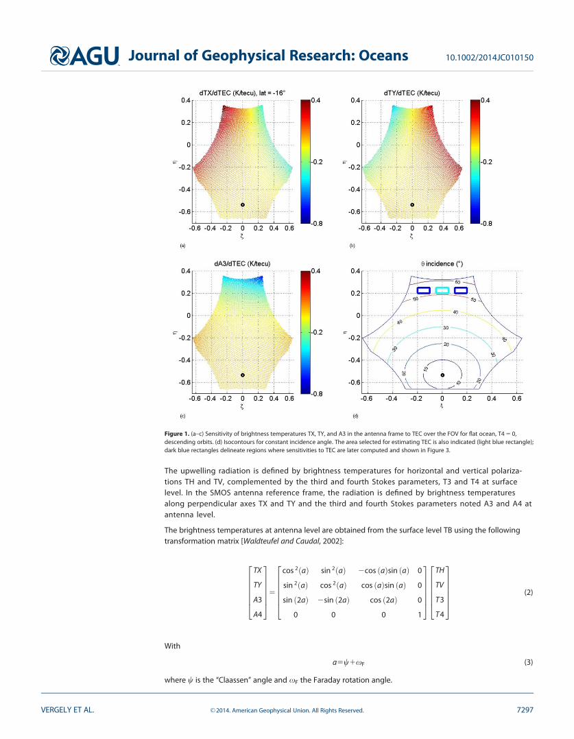
2.2. TB Sensitivity to TEC Over the Field of ViewWe now consider the field of view (FOV) of SMOS, in the antenna reference frame. The FOV limits, asdepicted in Figure 1, are mainly imposed by taking into account aliasing. Lines of constant incidence angles(Figure 1d) are circles centered on the nadir location.

Journal of Geophysical Research: Oceans 10.1002/2014JC010150


The upwelling radiation is defined by brightness temperatures for horizontal and vertical polariza-tions TH and TV, complemented by the third and fourth Stokes parameters, T3 and T4 at surfacelevel. In the SMOS antenna reference frame, the radiation is defined by brightness temperaturesalong perpendicular axes TX and TY and the third and fourth Stokes parameters noted A3 and A4 atantenna level.

The brightness temperatures at antenna level are obtained from the surface level TB using the followingtransformation matrix [Waldteufel and Caudal, 2002]:

TX

TY

A3

A4

2666664

3777775

5

cos 2 að Þ sin 2 að Þ 2cos að Þsin að Þ 0

sin 2 að Þ cos 2 að Þ cos að Þsin að Þ 0

sin 2að Þ 2sin 2að Þ cos 2að Þ 0

0 0 0 1

2666664

3777775

TH

TV

T3

T4

2666664

3777775

(2)

With

a5w1xF (3)

where w is the ‘‘Claassen’’ angle and xF the Faraday rotation angle.

Figure 1. (a–c) Sensitivity of brightness temperatures TX, TY, and A3 in the antenna frame to TEC over the FOV for flat ocean, T4 5 0,descending orbits. (d) Isocontours for constant incidence angle. The area selected for estimating TEC is also indicated (light blue rectangle);dark blue rectangles delineate regions where sensitivities to TEC are later computed and shown in Figure 3.



Assuming the upwelling Stokes T4 is negligible, the matrix becomes:

TX

TY

A3

A4

2666664

3777775

5

cos 2 að Þ:TH1sin 2 að Þ:TV2cos að Þsin að Þ:T3

sin 2 að Þ:TH1cos 2 að Þ:TV1cos að Þsin að Þ:T3

sin 2að Þ:TH2sin 2að Þ:TV1cos 2að Þ:T3

0

2666664

3777775

(4)

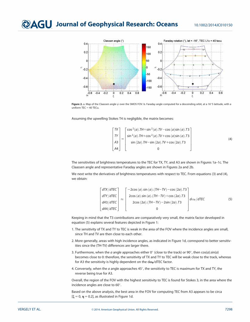
The sensitivities of brightness temperatures to the TEC for TX, TY, and A3 are shown in Figures 1a–1c. TheClaassen angle and representative Faraday angles are shown in Figures 2a and 2b.

We next write the derivatives of brightness temperatures with respect to TEC. From equations (3) and (4),we obtain:

dTX=dTEC

dTY=dTEC

dA3=dTEC

dA4=dTEC

2666664

3777775�

22cos að Þ:sin að Þ:ðTH2TVÞ2cos 2að Þ:T3

2cos að Þ:sin að Þ:ðTH2TVÞ1cos 2að Þ:T3

2cos 2að Þ: TH2TVð Þ22sin 2að Þ:T3

0

2666664

3777775

dxF=dTEC (5)

Keeping in mind that the T3 contributions are comparatively very small, the matrix factor developed inequation (5) explains several features depicted in Figure 1:

1. The sensitivity of TX and TY to TEC is weak in the area of the FOV where the incidence angles are small,since TH and TV are then close to each other.

2. More generally, areas with high incidence angles, as indicated in Figure 1d, correspond to better sensitiv-ities since the (TH-TV) differences are larger there.

3. Furthermore, when the a angle approaches either 0� (close to the track) or 90�, then cos(a).sin(a)becomes close to 0: therefore, the sensitivity of TX and TY to TEC will be weak close to the track, whereasfor A3 the sensitivity is highly dependent on the dxF/dTEC factor.

4. Conversely, when the a angle approaches 45�, the sensitivity to TEC is maximum for TX and TY, thereverse being true for A3.

Overall, the region of the FOV with the highest sensitivity to TEC is found for Stokes 3, in the area where theincidence angles are close to 60�.

Based on the above analysis, the best area in the FOV for computing TEC from A3 appears to be circa[n 5 0, g 5 0.2], as illustrated in Figure 1d.

Figure 2. a. Map of the Claassen angle w over the SMOS FOV. b. Faraday angle computed for a descending orbit, at a 16�S latitude, with auniform TEC 5 40 TECu.



It must be noted also that the sensitivity to TEC will decrease to zero when the angle between the line ofsight and magnetic field vector B is close to 90� .

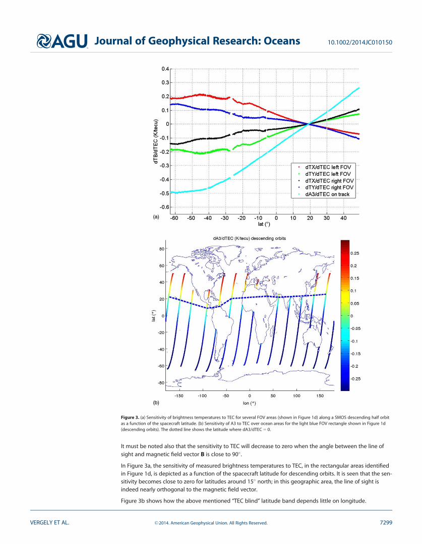
In Figure 3a, the sensitivity of measured brightness temperatures to TEC, in the rectangular areas identifiedin Figure 1d, is depicted as a function of the spacecraft latitude for descending orbits. It is seen that the sen-sitivity becomes close to zero for latitudes around 15� north; in this geographic area, the line of sight isindeed nearly orthogonal to the magnetic field vector.

Figure 3b shows how the above mentioned ‘‘TEC blind’’ latitude band depends little on longitude.

Figure 3. (a) Sensitivity of brightness temperatures to TEC for several FOV areas (shown in Figure 1d) along a SMOS descending half orbitas a function of the spacecraft latitude. (b) Sensitivity of A3 to TEC over ocean areas for the light blue FOV rectangle shown in Figure 1d(descending orbits). The dotted line shows the latitude where dA3/dTEC 5 0.



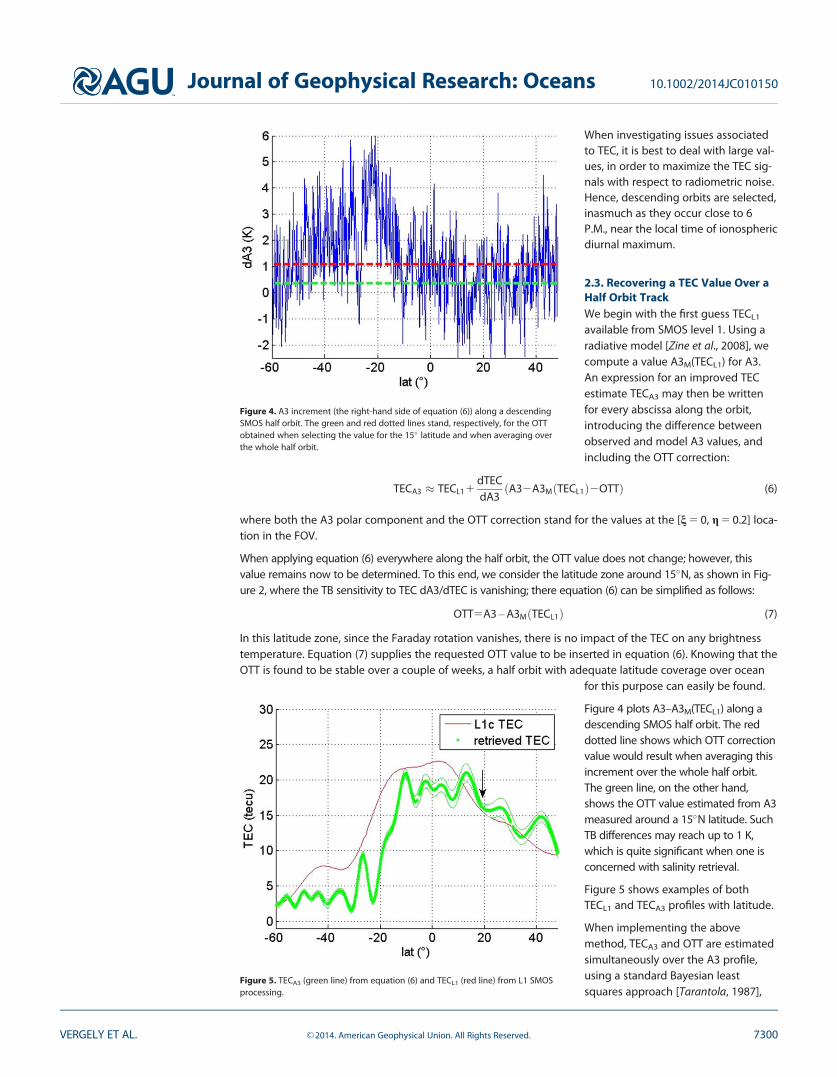
When investigating issues associatedto TEC, it is best to deal with large val-ues, in order to maximize the TEC sig-nals with respect to radiometric noise.Hence, descending orbits are selected,inasmuch as they occur close to 6P.M., near the local time of ionosphericdiurnal maximum.

2.3. Recovering a TEC Value Over aHalf Orbit TrackWe begin with the first guess TECL1

available from SMOS level 1. Using aradiative model [Zine et al., 2008], wecompute a value A3M(TECL1) for A3.An expression for an improved TECestimate TECA3 may then be writtenfor every abscissa along the orbit,introducing the difference betweenobserved and model A3 values, andincluding the OTT correction:

TECA3 � TECL11dTECdA3

ðA32A3MðTECL1Þ2OTTÞ (6)

where both the A3 polar component and the OTT correction stand for the values at the [n 5 0, g 5 0.2] loca-tion in the FOV.

When applying equation (6) everywhere along the half orbit, the OTT value does not change; however, thisvalue remains now to be determined. To this end, we consider the latitude zone around 15�N, as shown in Fig-ure 2, where the TB sensitivity to TEC dA3/dTEC is vanishing; there equation (6) can be simplified as follows:

OTT5A3 – A3MðTECL1Þ (7)

In this latitude zone, since the Faraday rotation vanishes, there is no impact of the TEC on any brightnesstemperature. Equation (7) supplies the requested OTT value to be inserted in equation (6). Knowing that theOTT is found to be stable over a couple of weeks, a half orbit with adequate latitude coverage over ocean

for this purpose can easily be found.

Figure 4 plots A3–A3M(TECL1) along adescending SMOS half orbit. The reddotted line shows which OTT correctionvalue would result when averaging thisincrement over the whole half orbit.The green line, on the other hand,shows the OTT value estimated from A3measured around a 15�N latitude. SuchTB differences may reach up to 1 K,which is quite significant when one isconcerned with salinity retrieval.

Figure 5 shows examples of bothTECL1 and TECA3 profiles with latitude.

When implementing the abovemethod, TECA3 and OTT are estimatedsimultaneously over the A3 profile,using a standard Bayesian leastsquares approach [Tarantola, 1987],

Figure 4. A3 increment (the right-hand side of equation (6)) along a descendingSMOS half orbit. The green and red dotted lines stand, respectively, for the OTTobtained when selecting the value for the 15� latitude and when averaging overthe whole half orbit.

Figure 5. TECA3 (green line) from equation (6) and TECL1 (red line) from L1 SMOSprocessing.



with TECL1 chosen as the a priorivalue. The TECA3 values retrievedalong track are smoothed using aGaussian filter with a 300 km width,in order to reduce noise. Around the‘‘TEC-blind’’ area, the algorithm tendsto retrieve the a priori value. Smallfluctuations present on the TECA3

curve are understood to be mostlydue to the remaining noise; theiramplitude is of the order of 3 TECu,depending on the latitude.

While the latitude indicated inabscissa in Figure 5 corresponds tothe location where the Spacecraft-to-Earth line of sight intersects the sur-face, it remains to determine whichlatitude ought to be assigned to theTECA3 values. The most adequatelocation (hence latitude) is the onewhere the bulk of ionospheric contri-

butions originates from, noting (from Figure 1d) that the incidence angle is about 50� . While the ionospherecannot be assimilated to a very thin horizontal layer, a simple Chapman layer model [Rishbeth and Garriott,1969] yields for the ionospheric F layer a mean altitude around 350 km (for a 20� sun incidence angle) anda standard deviation of the profile along the vertical of about 90 km (Figure 6). For a 60� incidence angle,the horizontal spread of the contributing layer then extends over 6150 km around the mean layer altitude.This allows defining the relevant latitude for each TEC estimate with an accuracy which is, at any rate, sub-stantially better than the latitudinal extent (circa 1200 km) of the SMOS geographical FOV.

As a consequence, while TEC values shown in Figure 5 are plotted for latitudes where the line of sight inter-sects the surface, the TECA3 profile should be assigned to latitudes shifted by about 5� northward.

2.4. TEC ComparisonsThe Figure 7a shows a map of TEC obtained from combined GPS files (ftp://cddis.gsfc.nasa.gov/gps/prod-ucts/ionex/) for 3 h Universal Time (UT). These files have actually been combined from contributions by sev-eral IGS Ionosphere Associate Analysis Centers [Hern�andez-Pajares, 2003]. The superimposed SMOS orbitshows that the descending half orbit occurs close to the daily maximum of the TEC in the middle afternoon,while the ascending one is close to the minimum.

The Figure 7b next shows a map of the same combined GPS files for the SMOS descending half orbit over427 descending orbits in May 2011, that is for a constant local time (LT) around 6 P.M.; Figure 7c presents asimilar 6 P.M. LT map for the TEC extracted using the A3 data.

While the bimodal maximum along a meridian was hardly visible on the UT map in Figure 7a, it nowappears as a major feature for both GPS TEC and TECA3 constant LT maps. This feature is mostly apparent inthe Pacific Ocean zones. It is more marked for TECA3 for which the spatial resolution induced by the smooth-ing function is about 300 km, while for the GPS data it is at best 550 km along a meridian, due to the stepof the interpolation grid.

We are observing here the well-known equatorial anomaly associated to the ‘‘equatorial fountain’’mechanism [e.g., Rishbeth and Garriott, 1969]: the combined effect of plasma diffusion along linesof the Earth’s magnetic field and motion across the field lines generated by an assumed distribu-tion of eastward electric field induces a deep ionospheric ‘‘trough’’ centered on the magneticequator.

At the global scale, an asymmetry is noted between the North and South hemispheres, for both TEC mapsin Figures 7b and 7c, with larger values in the North hemisphere. This might be expected at this time of

Figure 6. Representative ionospheric F layer using a Chapman photoionizationmodel with a constant 60 km scale height. The red thick line shows the mean alti-tude 61 standard deviation.



http://ftp://cddis.gsfc.nasa.gov/gps/products/ionex/

http://ftp://cddis.gsfc.nasa.gov/gps/products/ionex/

Figure 7. (a) Example of a global TEC map built from combined ionosphere map exchange (IONEX) GPS products. (b) Local time 18 h mapfor TEC derived from GPS data. (c) Local time 18 h map for TEC derived from SMOS Stokes 3.



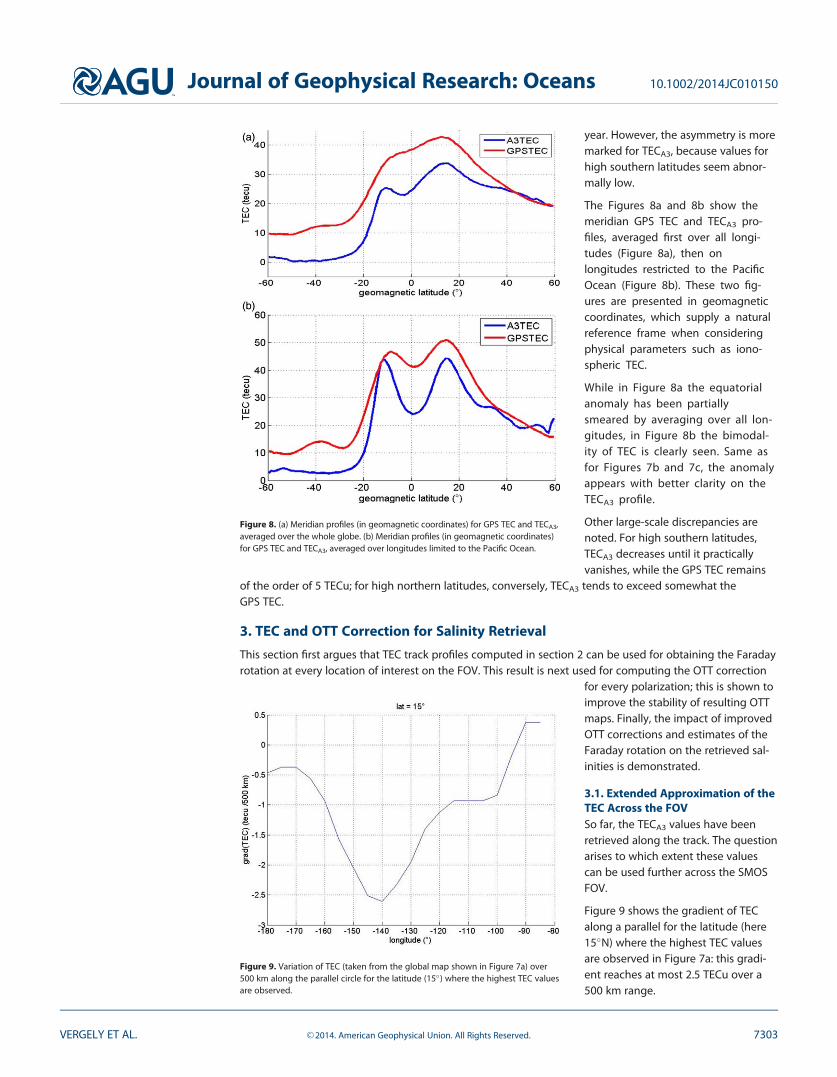
year. However, the asymmetry is moremarked for TECA3, because values forhigh southern latitudes seem abnor-mally low.

The Figures 8a and 8b show themeridian GPS TEC and TECA3 pro-files, averaged first over all longi-tudes (Figure 8a), then onlongitudes restricted to the PacificOcean (Figure 8b). These two fig-ures are presented in geomagneticcoordinates, which supply a naturalreference frame when consideringphysical parameters such as iono-spheric TEC.

While in Figure 8a the equatorialanomaly has been partiallysmeared by averaging over all lon-gitudes, in Figure 8b the bimodal-ity of TEC is clearly seen. Same asfor Figures 7b and 7c, the anomalyappears with better clarity on theTECA3 profile.

Other large-scale discrepancies arenoted. For high southern latitudes,TECA3 decreases until it practicallyvanishes, while the GPS TEC remains

of the order of 5 TECu; for high northern latitudes, conversely, TECA3 tends to exceed somewhat theGPS TEC.

3. TEC and OTT Correction for Salinity Retrieval

This section first argues that TEC track profiles computed in section 2 can be used for obtaining the Faradayrotation at every location of interest on the FOV. This result is next used for computing the OTT correction

for every polarization; this is shown toimprove the stability of resulting OTTmaps. Finally, the impact of improvedOTT corrections and estimates of theFaraday rotation on the retrieved sal-inities is demonstrated.

3.1. Extended Approximation of theTEC Across the FOVSo far, the TECA3 values have beenretrieved along the track. The questionarises to which extent these valuescan be used further across the SMOSFOV.

Figure 9 shows the gradient of TECalong a parallel for the latitude (here15�N) where the highest TEC valuesare observed in Figure 7a: this gradi-ent reaches at most 2.5 TECu over a500 km range.

Figure 8. (a) Meridian profiles (in geomagnetic coordinates) for GPS TEC and TECA3,averaged over the whole globe. (b) Meridian profiles (in geomagnetic coordinates)for GPS TEC and TECA3, averaged over longitudes limited to the Pacific Ocean.

Figure 9. Variation of TEC (taken from the global map shown in Figure 7a) over500 km along the parallel circle for the latitude (15�) where the highest TEC valuesare observed.



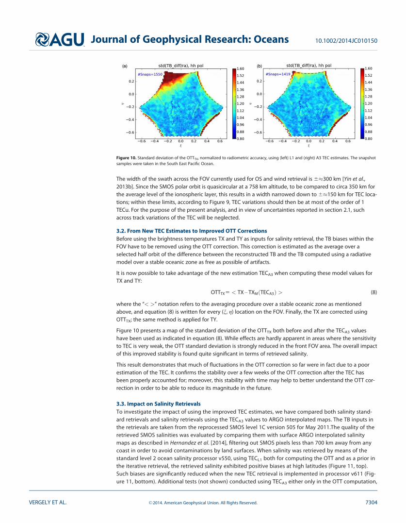
The width of the swath across the FOV currently used for OS and wind retrieval is 6�300 km [Yin et al.,2013b]. Since the SMOS polar orbit is quasicircular at a 758 km altitude, to be compared to circa 350 km forthe average level of the ionospheric layer, this results in a width narrowed down to 6�150 km for TEC loca-tions; within these limits, according to Figure 9, TEC variations should then be at most of the order of 1TECu. For the purpose of the present analysis, and in view of uncertainties reported in section 2.1, suchacross track variations of the TEC will be neglected.

3.2. From New TEC Estimates to Improved OTT CorrectionsBefore using the brightness temperatures TX and TY as inputs for salinity retrieval, the TB biases within theFOV have to be removed using the OTT correction. This correction is estimated as the average over aselected half orbit of the difference between the reconstructed TB and the TB computed using a radiativemodel over a stable oceanic zone as free as possible of artifacts.

It is now possible to take advantage of the new estimation TECA3 when computing these model values forTX and TY:

OTTTX5 < TX – TXM TECA3ð Þ > (8)

where the ‘‘< >’’ notation refers to the averaging procedure over a stable oceanic zone as mentionedabove, and equation (8) is written for every (n, g) location on the FOV. Finally, the TX are corrected usingOTTTX; the same method is applied for TY.

Figure 10 presents a map of the standard deviation of the OTTTX both before and after the TECA3 valueshave been used as indicated in equation (8). While effects are hardly apparent in areas where the sensitivityto TEC is very weak, the OTT standard deviation is strongly reduced in the front FOV area. The overall impactof this improved stability is found quite significant in terms of retrieved salinity.

This result demonstrates that much of fluctuations in the OTT correction so far were in fact due to a poorestimation of the TEC. It confirms the stability over a few weeks of the OTT correction after the TEC hasbeen properly accounted for; moreover, this stability with time may help to better understand the OTT cor-rection in order to be able to reduce its magnitude in the future.

3.3. Impact on Salinity RetrievalsTo investigate the impact of using the improved TEC estimates, we have compared both salinity stand-ard retrievals and salinity retrievals using the TECA3 values to ARGO interpolated maps. The TB inputs inthe retrievals are taken from the reprocessed SMOS level 1C version 505 for May 2011.The quality of theretrieved SMOS salinities was evaluated by comparing them with surface ARGO interpolated salinitymaps as described in Hernandez et al. [2014], filtering out SMOS pixels less than 700 km away from anycoast in order to avoid contaminations by land surfaces. When salinity was retrieved by means of thestandard level 2 ocean salinity processor v550, using TECL1 both for computing the OTT and as a prior inthe iterative retrieval, the retrieved salinity exhibited positive biases at high latitudes (Figure 11, top).Such biases are significantly reduced when the new TEC retrieval is implemented in processor v611 (Fig-ure 11, bottom). Additional tests (not shown) conducted using TECA3 either only in the OTT computation,

Figure 10. Standard deviation of the OTTTX, normalized to radiometric accuracy, using (left) L1 and (right) A3 TEC estimates. The snapshotsamples were taken in the South East Pacific Ocean.



or only as an improved auxiliary TEC data set when retrieving OS, did not show such improvements, con-firming the need to include TECA3 in both computations. It must however be stressed that the mainimprovement comes from the contribution of TECA3 when computing the OTT. This explains why, insome regions, retrieved OS values exhibit significant differences although the local TEC values undergolittle change.

Biases and standard deviations (std) of SMOS-ARGO salinity differences are reported in Table 1. Both meanbiases and std are reduced when the TEC estimated from A3 is introduced, whatever the region considered.In addition, with the TECA3 algorithm, std obtained during descending orbits become closer to those esti-mated for ascending orbits, within 10%, or even almost identical in tropical regions.

Figure 11. SMOS OS minus ARGO OS interpolated maps, May 2011, descending orbits. (top) SMOS OS retrieved with default L2 processorv550. (bottom) SMOS OS retrieved with the TECA3 as described in this paper. Note the improvement in the latitudinal bias.



4. Summary and Conclusions

Our sensitivity study has indicated that the A3 Stokes component (Stokes 3 in the antenna referenceframe) exhibits the highest sensitivity to TEC in the front part of the SMOS Field of View. We haveshown how it is possible to compute an improved OTT correction which yields a bias-free estimationof TEC over the whole half orbit track. While the computations have been performed with SMOS level1 data v505, the A3 OTT is expected to be much reduced with the updated L1 processor to bereleased in the near future, thanks to recent improvements in the image reconstruction algorithm.Hence, one could expect and hope that the magnitude of the OTT correction will decrease withfuture releases of the SMOS L1 data. For example, it is expected that the contamination of A3 bycross-polar contributions leaked from TX and TY [Wu et al., 2013] will be explicitly taken into accountby future versions of the processing chain, rather than being compensated by a part of the empiricalOTT correction.

We have compared SMOS-derived TEC to TEC maps based on GPS measurements. Overall satisfactoryagreement is found; the well-known equatorial anomaly is present and emphasized in the SMOS-derivedTEC, owing most probably to the better spatial resolution.

The new TEC estimation is used in turn to improve the pixel-dependent OTT correction for every polariza-tion component and location on FOV; the resulting correction clearly shows better stability. Finally, a betteragreement is obtained between retrieved salinities and ground truth data.

The TECA3 estimation should not however be considered as fully validated at this stage. Specifically, whilethe enhanced representation of the equatorial anomaly is encouraging, we have to validate it againstother TEC data with better spatial resolution than the maps built from GPS measurements. In this respectaltimetry data are obvious candidates, with better coverage over ocean surfaces.

In the same spirit, it is necessary to investigate the discrepancies for high latitudes, especially on the south-ern hemisphere where TECA3 values are found close to zero. Concerning the forward radiative model, the(TH-TV) differences might be incorrect due to an inadequacy of the roughness model in these high windregions, and/or of the dielectric model for cold waters known to prevail there; similarly, in such conditions,the upwelling Stokes 3 component might be larger than predicted. In depth investigations coordinatedwith the Aquarius team [Lagerloef et al., 2008] are called for. Interestingly, a test performed on Aquariusdata during the same season (although for a different year) indicates at first order a similar meridian distri-bution of TEC [Dinnat et al., 2014].

In the present paper, we have considered only the FOV region with the highest sensitivity to TEC. The tech-nique might be extended elsewhere on the FOV, giving access to TEC information obtained for a variety ofincidence angles. This deserves attention because it should allow us to optimize the altitude selected forthe equivalent ionospheric ‘‘slab’’ layer, and ultimately optimize the geographical localization for estimatedTEC values.

Finally, it is expected that the TEC itself obtained from SMOS may deserve to be investigated more in detail.For example, it is well known that magnetic storms induce strong disturbances in the ionospheric F2 layer[Rishbeth and Garriott, 1969] and thus the TEC behavior. Such phenomena should not be ignored when theTEC is introduced in the frame of corrections (which is the case, e.g., for SMOS and surface salinity); alterna-tively, TEC profiles obtained from SMOS might bring useful additional information on the effect of magneticstorms.

We have focused the present study on SMOS data collected over the oceans. True to say, the sensitivity con-ditions are such that the impact of ionospheric corrections is weaker over the continents. However, the

Table 1. SMOS OS From Descending Orbits Versus ARGO Interpolated OS Maps for May 2011

L2 V550 Processing: TECL1c Used Both asPrior and in OTT Computation

L2 V611 Processing: TECA3 Used Both asPrior and in OTT Computation

Zone Mean Std Zone Mean Std60�S 60�N 0.11 0.39 60�S 60�N 0.02 0.3645�S 45�N 0.05 0.32 45�S 45�N 0.01 0.2930�S 30�N 20.01 0.29 30�S 30�N 0.02 0.27



improvements discussed above, when achieved over oceans, will also be of benefit over the continentswhen estimating soil moisture and other surface parameters.

ReferencesBarton, C. E. (1997), International geomagnetic reference field: The seventh generation, J. Geomagn. Geoelectr., 49, 123–148.Claassen, J. P., and A. K. Fung (1974), The recovery of polarized apparent temperature distributions of flat scenes from antenna tempera-

ture measurements, IEEE Trans. Antennas Propag., AP-22, 433–442.Crapolicchio, R. (2008), VTEC usage for the SMOS Level 1 operational processor (L1-OP), ESA Tech. Note XSMS-GSEG-EOPG-TN-06–0019, ESA/

ESRIN, 00044 Frascati, Italy.Dinnat, E., et al. (2014), Comparison of SMOS and Aquarius Sea Surface Salinity and analysis of possible causes for the differences, paper

presented at XXXIst URSI General Assembly and Scientific Symposium, Beijing, 16–23 Aug, NASA-GSFC, Greenbelt, Md.Gutierrez, A. (2006), SMOS L1 processor Algorithm_Theoretical Baseline Definition, DEIMOS Tech. Note SO-DS-DME-L1PP-0011, 71 pp.,

DEIMOS Engenharia, Lisboa, Portugal.Hernandez, O., J. Boutin, N. Kolodziejczyk, G. Reverdin, N. Martin, F. Gaillard, N. Reul, and J. L. Vergely (2014), SMOS salinity in the subtropi-

cal north Atlantic salinity maximum: 1. Comparison with Aquarius and in situ Salinity, J. Geophys. Res., doi:10.1002/2013JC009610, inpress.

Hern�andez-Pajares, M. (2003), Performances of IGS ionosphere TEC maps, 7th IGS Iono WG report, Technical University of Catalonia,Barcelona, Spain.

Kerr, Y. H., et al. (2010), The SMOS mission: New tool for monitoring key elements of the global water cycle, Proc. IEEE, 98, 666–687.Kerr, Y. H., et al. (2012), The SMOS soil moisture retrieval algorithm, IEEE Trans. Geosci. Remote Sens., 50(5), 1384–1403.Lagerloef, G. S. E., et al. (2008), The Aquarius/SAC-D mission: Designed to meet the salinity remote sensing challenge, Oceanography, 21(1),

69–81.Le Vine, D. M., and S. Abraham (2000), Faraday rotation and passive microwave remote sensing of soil moisture from space, in Microwave

Radiometer Remote Sensing Earth’s Surface Atmosphere, edited by P. Pampaloni and S. Paloscia, pp. 89–96, VSP BV, Netherlands.Mecklenburg, S., et al. (2012), ESA’s soil moisture and ocean salinity mission: Mission performance and operations, IEEE Trans. Geosci.

Remote Sens., 50(5), 1354–1366.Reul, N., et al. (2013), Sea surface salinity observations from space with the SMOS satellite: A new means to monitor the marine branch of

the water cycle, Surv. Geophys., 35(3), 681–722.Rishbeth, H., and O. K. Garriott (1969), Introduction to Ionospheric Physics, 331 pp., Academic, N. Y.Tarantola, A. (1987), Inverse Problem Theory, Elsevier, N. Y.Waldteufel, P., and G. Caudal (2002), About off-axis radiometric polarimetric measurements, IEEE Trans. Geosci. Remote Sens., 40(6), 1435–

1439.Wu, L., F. Torres, I. Corbella, N. Duffo, I. Duran, M. Vall-llossera, A. Camps, D. Delwart, and M. Martin-Neira (2013), Radiometric performance

of SMOS full polarimetric imaging, Geosci. Remote Sens. Lett., 10(6), 1454–1458.Yin, X., J. Boutin, and P. Spurgeon (2012), First assessment of SMOS data over Open Ocean. Part I: Pacific Ocean, IEEE Trans. Geosci. Remote

Sens., 540(5), 1648–1661.Yin, X., J. Boutin, and P. Spurgeon (2013a), Biases between measured and simulated SMOS brightness temperature over ocean, IEEE J. Selec.

Top. Appl. Earth Obs. Remote Sens., 6(3), 1341–1350, doi:10.1109/JSTARS.2013.2252602.Yin, X., J. Boutin, N. Martin, P. Spurgeon, and J. Vergely (2013b), Errors in SMOS sea surface salinity and their dependency on a priori wind

speed, Remote Sens. Environ., 146, 159–171, doi:10.1016/j.rse.2013.09.008.Zine, S., J. Boutin, J. Font, N. Reul, P. Waldteufel, C. Gabarro, J. Tenerelli, F. Petitcolin, J. L. Vergely, and M. Talone (2008), Overview of the

SMOS sea surface salinity prototype processor, IEEE Trans. Geosci. Remote Sens., 46(3), 621–645, doi:10.1109/TGRS.2008.915543.

AcknowledgmentsThis work was supported in part byESRIN/contracts 1-6704/11/I-AM(SMOS1 polarimetry) and 3-13003/10/I-OL (SMOS phase E) and by CNES/TOSCA SMOS-OCEAN contract. We aregrateful to Elvira Astafyeva for helpfuldiscussions, to Nicolas Martin forperforming SMOS-ARGO collocations,and to Emmanuel Dinnat for carryingout an encouraging test on Aquariusdata. SMOS Level 1 and 2 data areavailable from ESA upon requestsubmitted to the EO help [email protected].



http://dx.doi.org/10.1002/2013JC009610

http://dx.doi.org/10.1109/JSTARS.2013.2252602

http://dx.doi.org/10.1016/j.rse.2013.09.008

http://dx.doi.org/10.1109/TGRS.2008.915543

Date post:	27-Nov-2021
Category:	Documents
Upload:	others
View:	1 times
Download:	0 times

New total electron content retrieval improves SMOS sea ...

Documents