35
Dr. Edward I. Altman Stern School of Business New York University
| Date post: | 14-Mar-2018 |
| Category: |
Documents |
| Upload: | phungtuong |
| View: | 213 times |
| Download: | 0 times |

Dr. Edward I. AltmanStern School of BusinessNew York University

2
Problems With Traditional Financial Ratio Analysis
1 Univariate Technique1-at-a-time
2 No “Bottom Line”
3 Subjective Weightings
4 Ambiguous
5 Misleading

3
Forecasting Distress With Discriminant AnalysisLinear Form
Z = a1x1 + a2x2 + a3x3 + …… + anxn
Z = Discriminant Score (Z Score)
a1 an = Discriminant Coefficients (Weights)
x1 xn = Discriminant Variables (e.g. Ratios)
Examplex
xx
xx
xx
xxx
x
x
x x x
xx
x
xx
x
x x
xx
x
x
x
xx
xx
x x
x
x
xxx
EBITTA
EQUITY/DEBT

4
“Z” Score Component Definitions
Variable Definition Weighting FactorX1 Working Capital 1.2
Total Assets
X2 Retained Earnings 1.4
Total Assets
X3 EBIT 3.3
Total Assets
X4 Market Value of Equity 0.6
Book Value of Total Liabilities
X5 Sales 1.0
Total Assets

5
Z ScoreBankruptcy Model
Z = .012X1 + .014X2 + .033X3 + .006X4 + .999X5
e.g. 20.0%
Z = 1.2X1 + 1.4X2 + 3.3X3 + .6X4 + .999X5
e.g. 0.20
X1 = Current Assets - Current Liabilities X4 = Market Value of EquityTotal Assets Total Liabilities
X2 = Retained Earnings X5 = Sales (= # of Times
Total Assets Total Assets e.g. 2.0x)
X3 = Earnings Before Interest and Taxes
Total Assets
6
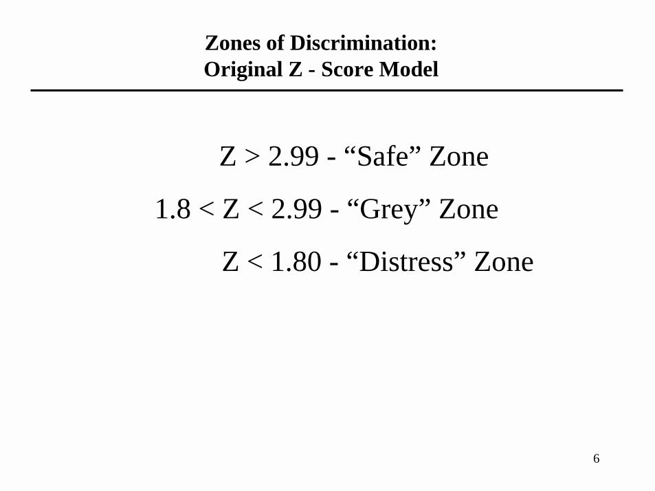
Zones of Discrimination:Original Z - Score Model
Z > 2.99 - “Safe” Zone
1.8 < Z < 2.99 - “Grey” Zone
Z < 1.80 - “Distress” Zone

7
Classification & Prediction AccuracyZ Score (1968) Failure Model*
1969-1975 1976-1995 1997-1999Year Prior Original Holdout Predictive Predictive PredictiveTo Failure Sample (33) Sample (25) Sample (86) Sample (110) Sample (120)
1 94% (88%) 96% (72%) 82% (75%) 85% (78%) 94% (84%)
2 72% 80% 68% 75% 74%
3 48% - - - -
4 29% - - - -
5 36% - - - -
*Using 2.67 as cutoff score (1.81 cutoff accuracy in parenthesis)

8
Z Score Trend - LTV Corp.
-1.5-1
-0.50
0.51
1.52
2.53
3.5
1980 1981 1982 1983 1984 1985 1986
Year
Z Sc
ore
Grey Zone
Bankrupt
July ‘86
Safe Zone
Distress Zone
2.99
1.8

9
International Harvester (Navistar)Z Score (1974 - June 1996)
-0.50
0.51
1.52
2.53
3.5
'74 '76 '78 '80 '82 '84 '86 '88 '90 '92 '94 '96Year
Z Sc
ore
Safe Zone
Grey Zone
Distress Zone

10
Chrysler CorporationZ Score (1976 - June 1996)
00.5
11.5
22.5
33.5
4
'76 '78 '80 '82 '84 '86 '88 '90 '92 '94 '96
Year
Z Sc
ore
Consolidated Co.
Operating Co.
Gov’t Loan Guarantee
Safe Zone
Grey Zone

11
IBM CorporationZ Score (1980 - June 1997)
00.5
11.5
22.5
33.5
44.5
55.5
6
1980 1982 1984 1986 1988 1990 1992 1994 1996
Year
Z Sc
ore
Operating Co.Safe Zone
Consolidated Co.
Grey Zone BBB
BB
B 1/93: Downgrade AAA to AA-
July 1993: Downgrade AA- to A

12
Average Z-Score by S&P Bond RatingS&P 500: 1992 - 1995 *
11 5.020 1.603 4.376 1.380 4.506 1.499 5.263 2.194
46 4.296 1.911 4.047 1.832 4.032 1.893 4.226 2.088
131 3.613 2.259 3.472 2.007 3.607 2.180 3.923 3.255
107 2.776 1.493 2.701 1.580 2.839 1.741 2.601 1.535
30 2.449 1.623 2.276 1.694 2.185 1.626 2.102 1.544
80 1.673 1.234 1.876 1.517 1.964 1.716 1.962 2.333
AAA
AA
A
BBB
BB
B
Num. Of Std. Std. Std. Std.
Firms Avg. Dev. Avg. Dev. Avg. Dev. Avg. Dev.
1995 1994 1993 1992
*

13
Xerox Credit Quality: Z Score Analysis 1998-2000
3.46
2.38
1.35
-
0.50
1.00
1.50
2.00
2.50
3.00
3.50
4.00
12/98 12/99 6/00
Z-Sc
ore
Bond Rating Equivalents: Actual Rating (S&P):12/98 A 12/98 A12/99 BB 12/99 A06/00 B 06/00 A
12/00 BBB-

14
Z’ ScorePrivate Firm Model
Z’ = .717X1 + .847X2 + 3.107X3 + .420X4 + .998X5
X1 = Current Assets - Current Liabilities
Total Assets
X2 = Retained Earnings
Total Assets
X3 = Earnings Before Interest and Taxes
Total Assets
X4 = Book Value of Equity Z’ > 2.90 - “Safe” Zone
Total Liabilities 1.23 < Z’ < 2.90 - “Grey” Zone
X5 = Sales Z’ < 1.23 - “Distress” Zone
Total Assets

15
Z’’ Score Model for Manufacturers, Non-Manufacturer Industrials, & Emerging Market Credits
Z’’ = 6.56X1 + 3.26X2 + 6.72X3 + 1.05X4
X1 = Current Assets - Current Liabilities
Total Assets
X2 = Retained Earnings
Total Assets
X3 = Earnings Before Interest and Taxes
Total Assets
X4 = Book Value of Equity Z’’ > 2.60 - “Safe” Zone
Total Liabilities 1.1 < Z’’ < 2.60 - “Grey” Zone
Z ” < 1.1 - “Distress” Zone

16
Circle K - Z Score (1979 - 1992)
0
1
2
3
4
5
6
7
'79 '80 '81 '82 '83 '84 '85 '86 '87 '88 '89 '90 '91 '92
Year
Z S
core Safe Zone
Grey Zone
BankruptMay ‘90

17
Amazon.com Z-Scores 1998-2000Five Variable Model With Market Value Equity (X4)
(4)
(2)
-
2
4
6
8
10
Mar
-98
May
-98
Jul-9
8
Sep
-98
Nov
-98
Jan-
99
Mar
-99
May
-99
Jul-9
9
Sep
-99
Nov
-99
Jan-
00
Mar
-00
May
-00
Jul-0
0
Sep
-00
Nov
-00
SAFE ZONE
DISTRESS ZONE

18
Amazon.com Z-Scores 1997-2000Four Variable Model With Book Value Equity (X4)
(6)
(4)
(2)
-
2
4
6
Jun-97
Sep-97
Dec-97
Mar-98
Jun-98
Sep-98
Dec-98
Mar-99
Jun-99
Sep-99
Dec-99
Mar-00
Jun-00
Sep-00
Dec-00
SAFE ZONE
DISTRESS ZONE

19
DAF Corporation Z Scores(Dutch Company Bankruptcy 1993)
1.75
2.15
1.53
1.000.80
0
0.5
1
1.5
2
2.5
Z Sc
ore
1987 1988 1989 1990 1991Year

20
Average Z-Scores: US Industrial Firms1975-1999
0
2
4
6
8
10
12
Mar-75
Mar-77
Mar-79
Mar-81
Mar-83
Mar-85
Mar-87
Mar-89
Mar-91
Mar-93
Mar-95
Mar-97
Mar-99
Mean

21
Argenti (A Score System)Defects
In ManagementWeight
8 - Chief Executive is an autocrat4 - He is also the chairman2 - Passive Board - an autocrat assures this2 - Unbalanced Board - too many engineers or too many finance types1 - Poor management depth
In Accountancy3 - No budgets or budgetary controls3 - No cash flow plans, or not updated3 - No costing system. Cost and contribution of each product
unknown15 - Poor response to change, old fashioned product, obsolete factory,
out-of-date marketing Total Defects 42 Pass 10

22
Argenti (A Score System)Symptoms
Weight5 - Financial signs, such as Z Score4 - Creative accounting. Chief executive is the first to see signs of
failure, and in an attempt to hide it from creditors and the banks, accounts are ‘glossed over’ by overvaluing stocks, using lower depreciation, etc.
3 - Non-financial signs, such as untidy offices, frozen salaries, chief executive ‘ill’, high staff turnover, low morale, rumors
1 - “Terminal signs”Total Symptoms 13Total Possible Score 100 Pass 25
Total Score Prognosis0-10 No Worry (High Pass)0-25 Pass10-18 Cause for Anxiety (Pass)18-35 Grey Zone - Warning Sign>35 Company “At Risk”

24
KMV Credit Monitor Model
• Provides a quantitative assessment of the credit risk of publicly traded companies
• The model is theoretically rather than empirically based
• It is built around the market’s valuation of a firm’s creditworthiness
• The model can be applied to the universe of publicly-traded companies
• The universe consists of thousands of companies in the U.S.
• By contrast, only approximately 2000 companies have publicly-traded debt that is rated by the rating agencies. Even then, bond price data is often difficult to get.

25
The Market’s Valuation of Debt
• The stock market’s perception of the value of a firm’s equity are readily conveyed in a traded company’s stock price
• The information contained in the firm’s stock price and balance sheet can be translated into an implied risk of default through two relationships:
• The relationship between the market value of a firm’s equity and the market value of its assets.
• The relationship between the volatility of a firm’s assets and the volatility of a firm’s equity.

26
KMV Credit Monitor Output
• A quantitative estimate of the default probability called the expected default frequency (EDF).
• EDFs are calibrated to measure the probability of a borrower defaulting within one year.
• EDFs are reported in percentages ranging from 0 to 20.

27
KMV Model - Empirical Result
STEP 1 - Model Estimates Market Value and Volatility of Firm’s Assets
STEP 2 - Then calculates the Distance-to-Default (# of Standard Deviations)
Distance-to-Default is a Type of Asset/Liability Coverage Ratio
STEP 3 - Distance-to-Default of a Firm is Mapped Against a Database of Empirical Frequencies of Similar Distance-to-Default Companies to Obtain Expected Default Frequency (EDF) for a Firm

28
Estimation of Market Value And Volatility of Firm’s Assets
• Asset Values are Based on Underlying Value of Firm, Independent of Firm’s Liabilities.
• Asset Volatility Calculated as the Annualized Standard Deviation of Percentage Changes in the Market Value of Assets.
• Equity Market Value and its Volatility, as Well as the Liability Structure, are Used as Proxies for the Asset’s Value and Volatility.
• Option Theory of Assets Used to Value Assets Since MV of Debt is Not Known. If Debt MV is Known, then A=E+D (MV). But, MV Assets are Calculated by Knowing Only the MV Equity and PV of Liabilities.

29
Estimation of Market Value And Volatility of Firm’s Assets
(continued)
• KMV Assumes that All Short Term Debt and 50% of Long Term Liabilities Are Used to Calculate the Default Point (Was 25% of LTD).
• When MV Assets < Payable Liabilities then Firm Defaults. Firm Cannot Sell Off Assets or Raise Additional Capital Because All Existing Assets are Fully Encumbered.

30
KMV Strengths
• Can be applied to any publicly-traded company
• Responsive to changing conditions, (EDF updated quarterly)
• Based on stock market data which is timely and contains a forward looking view
• Strong theoretical underpinnings (versus ad-hoc models)

31
KMV Weaknesses
• Difficult to diagnose a theoretical EDF (what is the distribution of asset return outcomes)
• Problems in applying model to private companies and thinly-traded companies
• Results sensitive to stock market movements (does the stock-market over-react to news?)
• Ad-hoc definition of anticipated liabilities (ie. 50% of long-term debt)

32

33
KMV’S Expected Default Frequency (EDF)
Based on empirical observation of the Historical Frequency of the Number of Firms that Defaulted With Asset Values (Equity + Debt) Exceeding Face Value of Debt Service By a Certain Number of Standard (Std.) Deviations at one year prior to default.For Example:
Current Market Value of Assets = $ 910Expected One Year Growth in Assets = 10%Expected One Year Asset Value = $1,000Standard Deviation = $ 150Par Value of Debt Service in One Year = $ 700
Therefore:# Std. Deviations from Debt Service = 2
Expected Default Frequency (EDF)Number of Firms that Defaulted With Asset Values 2 Std. Deviations from Debt Service
Total Population of Firms With 2 Std. Deviations from Debt Service
eg. = 50 Defaults = .05 = EDF1,000 Population
EDF =

34
Comparing Z-Score and KMV-EDF Bond Rating Equivalents
IBM Corporation

35
Diversification Based on Stock-Market Correlations (KMV)
• Uses Contingent Claims Approach based on the level and volatility of common stock prices to assess the value of the equity and its potential distribution. Compare that distribution of equity values plus the level of debt (total assets) to the anticipated debt level in the future in order to attain the probability of default (assets < liabilities). Losses based on expected recoveries.
• Assess the correlation of each loan’s expected return based on correlations of stock prices and the unexpected losses from different combination of Loans.
• Observes the possible Sharpe Ratios (expected return spread / unexpected loss) on various combinations of loans with differential investments (weight) in each loan.
• Stipulates the official frontier portfolio.


