Nexus between Climate Change and Food security in the...

Nexus between Climate Change and Food security in the East Africa Region: An Application of

Autoregressive Modelling Approach

Dennis O. Olila*, Vivian Oliver Wasonga

University of Nairobi

College of Agriculture and Veterinary Sciences

P.O.BOX 29053-00625, NAIROBI

Department of Land Resource Management & Agricultural Technology

Corresponding author*: [email protected]

Invited Paper Presented at the Fifth African Higher Education Week and Ruforum Biennial

Conference, 17 – 21 October, 2016, Cape Town, South Africa.

mailto:[email protected]

2 | P a g e

Abstract

This study is an attempt to unpack the existing link between climate change variability and food

security in the East Africa Community (EAC) region. Specifically, the paper elaborates the main

issues in climate change discourse and its implication to the food security equation in the EAC

region. A plethora of empirical literature exists in the area of climate change not only at the regional

level but also globally. Using secondary time series panel data, the study links cereal production

patterns with rainfall and temperature dynamics for from 1961 to 2012. The data was obtained from

the Food and Agricultural organization (FAOSTAT) as well as the World Bank knowledge

management center. Econometric data analysis was attained using Eviews version 7 and GMDH

version 3.8.3 statistical software. The findings of the Autoregressive model indicates that rainfall

and temperature are inevitably changing. These findings offer important policy insights on the role

played by climate change variability on food security in the EAC region.

Key words: Time series, Autoregressive modelling, rainfall, temperature, Kenya

3 | P a g e

1. Introduction

1.1 Background information

The phenomenon of climate change and variability has drawn a lot of attention among policy

makers and development partners. In their recent publication, the World Bank (2016) opine that

climate change and poverty alleviation present a huge challenge to the global community. Climate

change and variability is already causing negative impacts in many parts of the world (Jat et al.,

2012) particularly in Sub-Sahara Africa that is most vulnerable owing to the fact that over 70

percent of the population deriving their livelihoods from agriculture and natural based resource

activities (Antwi, 2013).

According to the Intergovernmental Panel on Climate Change (IPCC, 2001), the world has

witnessed rising temperatures during the last four decades in the lowest 8 kilometers of the

atmosphere. The aforementioned phenomenon is of great concern not only to policy makers but

also to development partners and various Non-Governmental Organizations (NGO’s) working in

the area of climate change and variability. From a global perspective, there is a unanimous

agreement that mitigation of negative impacts of climate change calls for cooperation among all

countries in the world (UNCCC, 1992).

The African continent is no exception to climate change and variability. As observed by United

Nations Framework Convention on Climate Change (UNFCCC, 2006), many African regions

perhaps experience variable climates coupled with intra-seasonal to decadal timelines. Empirical

evidence shows that climate change curtails sustainable economic and socioeconomic development

(Viljoen, 2013). The African continent exhibits high physical sensitivity to climate change (Antwi,

2013). For instance, African Progress Report (APP, 2015) posit that factors such as poverty,

dependence on rain-fed agriculture, weak infrastructure; both soft and hard part, as well as limited

provision of safety nets are some of the factors that contribute to vulnerability.

Alarmingly, the poor and marginalized, including subsistence farmers in rural Africa are likely to

face the worst consequences (CUTS, 2014). It is now clear that both rainfall and temperature

variability impacts negatively on food production, water resources, biodiversity, human and

livestock populations (Antwi, 2013). In the EAC region, nearly 70 percent of the population live

in rural areas where agriculture is the main source of livelihood.

4 | P a g e

Despite the high dependence on agriculture by rural livelihoods, climate change and variability

continues to jeopardize economic development of such communities. This is pegged on the fact

that climatic variables such as temperature, radiation, precipitation, humidity among others have a

direct impact on the productivity of agriculture, forestry and fishery systems (Antwi, 2013).

It is today common knowledge that climate change and variability is perhaps one of the major

challenges facing the world particularly the EAC region where agriculture remains a key economic

activity among a majority of the farmers. Antwi (2013) opine that climate change affects

agriculture in a number of ways including yield reduction, rising food prices, increased incidence

of pests and diseases, water scarcity, enhanced drought periods, soil fertility reduction, high cost

of livestock production, as well as creating tensions among the displaced persons.

According to Antwi (2013), the changes on agricultural production will impact on food security.

Specifically, reduced yield will affect food supply, and all forms of agricultural production will

negatively impinge on livelihoods and capacity to access food. This problem will be exacerbated

by the fact a majority of livelihoods are socially excluded from development.

The negative impacts of climate change and variability have been studied widely locally, regionally

and globally. For instance, EAC is cognizant of the fact that every major social, economic as well

as environmental sector is sensitive to climate change and variability. According to the EAC Food

Security Action Plan 2010 – 2015, the EAC region is frequently affected by food shortages and

pockets and hunger despite the huge potential and capacity to produce sufficient food for regional

consumption and export (East African Community Secretariat, 2010). These challenges emanates

from poor market integration which negatively affects trade flow as well as climate change and

variability.

In regard to the aforementioned challenges, the EAC food security action plan was formulated with

the aim of addressing the challenges of food insecurity in the region (East African Community

Secretariat, 2010). This development is in line with the EAC Treaty regarding cooperation in

agriculture and rural development in the achievement of food security and rational agricultural

production. Agricultural production, processing and preparation sector remain key in various EAC

member states. According to East African Community Secretariat (2010), between 70 to 80 percent

of the EAC labour force are involved in agriculture; which contributes between 24 and 48 percent

of the Gross Domestic Product (GDP).

5 | P a g e

However, despite the aforementioned attempts geared towards stabilizing food security in the EAC

region, the link between climate change and food security has received limited attention. Cognizant

of the fact that climate change and variability are expected to compromise agricultural production

and food security, it is envisaged that the findings of this study will go along in augmenting various

initiatives already put in place to address climate change and food insecurity in the EAC region.

Specifically, the study reveals long term patterns of rainfall and temperature and establishes how

these key climatic variables influence cereal production in the EAC region. Second, we forecast

rainfall, temperature and cereal production in order to offer ex-ante policy information on how

climate change is likely to compound the regions high poverty levels.

2. Methodology

2.1 Data

The study uses time series secondary data of rainfall and temperature patterns from Kenya, Uganda,

Tanzania and Burundi. The data was obtained from the World Bank Knowledge Management

center and from the Food and Agricultural Organization (http://faostat3.fao.org/home/E) of the

United Nations. The data ranges from the year 1961 – 2012.

3.1 Model specification

A time series is a collection of observations made sequentially through time (Chatfield, 2000).

Generally, these observations are spaced at equal time intervals. The main objective of analysis of

time series data is to find a mathematical model capable of explaining data behavior. For instance,

Olila and Wasonga (2016) analyzed time series data on carbon dioxide emission by Savanna

grasslands in Kenya. A growing interest in comprehending the behavior emanates from the need

to predict the future values of the series. Understanding the future values (forecasts) of time series

data is vital for ex-ante policy making and planning.

According to Chatfield (2000), time series data provides an excellent opportunity to look at out of

sample behavior (forecasted values) thus providing an opportunity to benchmark with the actual

observations. For instance, forecasting of GHG emissions enables formulation of appropriate

policies aimed at reducing emissions thus enhancing efficient decision-making. The objective of

this study is three fold.

http://faostat3.fao.org/home/E

6 | P a g e

First is to describe the emission data by plotting the actual values and make sense out of the pattern.

Having depicted the pattern clearly, the next objective undertaken by this study is to find a suitable

model to describe the data generating process. Finally, the study envisages estimating future values

(forecasting) of carbon emissions with the assumption that no action is taken to revert the

emissions.

From econometric context, we use an autoregressive (AR) model. In an AR (1) model, the variable

is regressed on itself by one lag period. Chatfield (2000) stipulates that a process xt is said to be

an autoregressive process of order p (abbreviated pAR ) if it is a weighted linear sum of the past

p values plus a random shock formulated as:

zxxxx tptpttt

...2211

........................................................................................ (1)

Where ztdenotes a purely random process with zero mean and variance

2

z and t denotes time.

Using the backward shift2 operator B such that xBx tt 1 , the pAR may be written more

succinctly in the form:

zx ttB .................................................................................................................................. (2)

Where Bp

pBB ...1 2

21 is polynomial in B of order .p According to Chatfield

(2000), the properties of AR processes defined by equation (1) is examined by focusing on the

properties of the function . Since B is an operator, the algebraic properties of have to be

investigated by examining the properties of x , where x denotes a complex variable rather than

by looking at B . It can be shown that equation (2) has a unique causal stationarity solution if the

roots of 0x lie outside the unit circle. This solution may be expressed as follows:

zx jtj

jt

0

........................................................................................................................... (3)

Taking into cognizance that for some constants jshould conform to .

j Equation (3)

above simply postulates that AR process is stationary provided the roots of 0x lie outside the

unit circle. The simplest example of an AR process is the first order case formulated as:

zxx ttt

1 .............................................................................................................................. (4)

7 | P a g e

The times series literature stipulates that an AR (1) process is stationarity provided that 1 is

satisfied. It is more accurate to say that there is a unique stationary solution of (4) which is causal,

provided that 1 . The autocorrelation function (ac.f) of a stationary AR (1) process is given by

k

k for nk ,...2,1 (Chatfield, 2000). Note that for a higher order stationary AR processes, the

ac.f will typically be a mixture of terms which decrease exponentially of damped sine or cosine

waves.

According to Nemec (1996), ac.f is a convenient way of summarizing the dependence between

observations in a stationary time series. In order to obtain ACF, a set of difference equations

commonly referred to as Yule-Walker equations are applied. Yule-Walker equation is formulated

as:

pkkkkk

...2211

......................................................................................... (5)

for ,,...2,1 nk 00 . One of the important useful property of AR process is the ability to show

that the partial ac.f is zero at all lags greater than ; implying that the sample ACF can be used to

determine the order of an AR process.

This is done by focusing the lag value at which the sample’s partial ac.f’s “cuts-off” i.e. should be

approximately zero or at least not significantly different from zero for higher lags (Chatfield, 2000).

4. Results and discussions

4.1 Kenya’s rainfall and temperature patterns

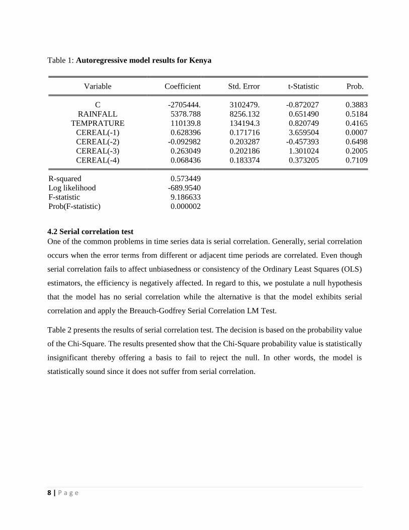
Table 1 shows the results of the autoregressive model. The dependent variable is cereal production

while the explanatory variables are rainfall, temperature and the lag of the cereal by four periods.

Based on the presented results, the first lag of cereal is statistically significant at one percent.

AR forecasting requires the dependent variable to fulfil some model parameter criteria such as (i)

the R-square value should be very high; (ii) there should be no serial correlation; (iii) no

heteroskedasticity and (iv) and the residual should follow a normal distribution. It is only after

validating the aforementioned that forecasting can be done.

In terms of our results, the lag of cereal is statistically significant at one percent (p-value = 0.000);

conforming to one of the most key requirement in time series forecasting. Moreover, our R-square

is slightly high (R-Square = 0.573); implying that over 50 percent variation in the dependent

variable is attributed to the dependent variables included in the model. Nevertheless, the F-statistic

and the corresponding probability is statistically significant at one percent (p-value = 0.000).

8 | P a g e

Table 1: Autoregressive model results for Kenya

Variable Coefficient Std. Error t-Statistic Prob.

C -2705444. 3102479. -0.872027 0.3883

RAINFALL 5378.788 8256.132 0.651490 0.5184

TEMPRATURE 110139.8 134194.3 0.820749 0.4165

CEREAL(-1) 0.628396 0.171716 3.659504 0.0007

CEREAL(-2) -0.092982 0.203287 -0.457393 0.6498

CEREAL(-3) 0.263049 0.202186 1.301024 0.2005

CEREAL(-4) 0.068436 0.183374 0.373205 0.7109

R-squared 0.573449

Log likelihood -689.9540

F-statistic 9.186633

Prob(F-statistic) 0.000002

4.2 Serial correlation test

One of the common problems in time series data is serial correlation. Generally, serial correlation

occurs when the error terms from different or adjacent time periods are correlated. Even though

serial correlation fails to affect unbiasedness or consistency of the Ordinary Least Squares (OLS)

estimators, the efficiency is negatively affected. In regard to this, we postulate a null hypothesis

that the model has no serial correlation while the alternative is that the model exhibits serial

correlation and apply the Breauch-Godfrey Serial Correlation LM Test.

Table 2 presents the results of serial correlation test. The decision is based on the probability value

of the Chi-Square. The results presented show that the Chi-Square probability value is statistically

insignificant thereby offering a basis to fail to reject the null. In other words, the model is

statistically sound since it does not suffer from serial correlation.

9 | P a g e

Table 2: Breusch-Godfrey Serial Correlation LM Test

F-statistic 1.524894 Prob. F(2,39) 0.2303

Obs*R-squared 3.481344 Prob. Chi-Square(2) 0.1754

Figure 1: Partial autocorrelation (PAC) and Autocorrelation (AC) for Kenya’s temperature

After carrying out serial correlation test, the final step was to identity the AR model. The shaded

area is the 95 percent confidence interval. The model for temperature is AR (3) while that for

rainfall is AR (2).

Figure 2: PAC and AC of Kenya’s rainfall pattern

-0.6

0-0

.40

-0.2

00

.00

0.2

0

Pa

rtia

l a

uto

co

rrela

tio

ns o

f D

.Ln_

tem

pra

ture

0 5 10 15 20 25Lag

95% Confidence bands [se = 1/sqrt(n)]

-0.6

0-0

.40

-0.2

00

.00

0.2

00

.40

Au

tocorr

ela

tion

s o

f D

.Ln

_te

mp

ratu

re

0 5 10 15 20 25Lag

Bartlett's formula for MA(q) 95% confidence bands

-0.4

0-0

.20

0.0

00

.20

0.4

00

.60

Pa

rtia

l a

uto

co

rrela

tio

ns o

f D

.Ln_

rain

fall

0 5 10 15 20 25Lag


-0.4

0-0

.20

0.0

00

.20

0.4

0

Au

tocorr

ela

tion

s o

f D

.Ln

_ra

infa

ll

0 5 10 15 20 25Lag


10 | P a g e

4.3 Cereal, rainfall and temperature forecast results for Kenya

Figure 3 presents the results of cereal, rainfall and temperature forecasting. The grey line indicates

the actual variability of cereal production, rainfall and temperature patterns from the year 1961 to

2012. It indicates that Kenya has been experiencing rainfall and temperature variability which

imposes a negative impact on cereal production. On the other hand, blue line shows the model fit

while the while the red line is the predicted cereal, rainfall and temperature patterns. On average,

Kenya’s cereal production has been on the rise from 1961 to 1912 despite the fluctuations partly

attributed to variability of rainfall and temperature patterns.

In terms of prediction, empirical results show that cereal production in Kenya will continue to

increase from 4.0 million in 2012 to 6.2 million Tons in 2021; representing a 55 percent increase

during this period. This will be attributed to a sharp decline in rainfall and an increase in

temperature as shown indicated in the figures below. By 2023, it is envisaged that the drop in cereal

production by approximately 65 percent by 2024 is likely to impact negatively on food security in

Kenya.

11 | P a g e

Figure3: Cereal, rainfall and temperature forecast respectively for Kenya

12 | P a g e

4.2 Uganda’s Cereal, rainfall and temperature patterns

Table 3 shows the model for Uganda’s cereal, rainfall and temperature patterns. Based on these

findings, AR (1) is the most suitable model for Uganda time series data. The adjusted R-squared

show that the independent variables explain 91 percent variation in the dependent variable.

Table 3: Autoregressive [AR (1)] model results for Uganda


C -1205604. 535021.1 -2.253376 0.0296

RAINFALL 6846.091 4009.055 1.707657 0.0953

TEMPRATURE 31756.72 19467.81 1.631242 0.1105

CEREAL(-1) 0.730456 0.154988 4.712992 0.0000

CEREAL(-2) 0.163590 0.192363 0.850421 0.4000

CEREAL(-3) 0.108122 0.191958 0.563261 0.5763

CEREAL(-4) -0.017391 0.158517 -0.109713 0.9132

R-squared 0.929742

Adjusted R-squared 0.919461



Further, the study tested for the existence of serial correlation in the data using Breusch-Godfrey

Serial Correlation LM test. Since the Chi-Square probability value is statistically insignificant,

we conclude fail to reject the null hypothesis of no serial correlation.

Table 4: Breusch-Godfrey Serial Correlation LM test



The results indicating the order of AR is as indicated in the figures (3) and (4) below. Results show

that Uganda time the time series temperature data follows and AR (1) model while rainfall data is

an AR (2) model.

13 | P a g e

Figure 3: PAC and AC for Uganda respectively for temperature

Figure 4: PAC and AC for Uganda respectively for rainfall

Having done the preliminary results in terms of checking for serial correlation and identifying the

model, the next step was to forecast the theme series data on the aforementioned parameters and

deduce the link between them. Specifically, we forecast cereal, rainfall and temperature patterns

and identify if they are correlated with each other. The results are indicated in figure 5 below.

The forecasted results for Uganda indicate that the country has been facing very minimum

fluctuations in cereal production between 1961 and 2012 despite the variability in rainfall. This

positive progress can be attributed to the increasing demand of cereals from Uganda by countries

-0.6

0-0

.40

-0.2

00

.00

0.2

0

Pa

rtia

l a

uto

co

rrela

tio

ns o

f D

.Ln_

tem

pra

ture

0 5 10 15 20 25Lag


-0.6

0-0

.40

-0.2

00

.00

0.2

00

.40

Au

tocorr

ela

tion

s o

f D

.Ln

_te

mp

ratu

re

0 5 10 15 20 25Lag


-0

.50

0.0

00

.50

1.0

0

Pa

rtial a

uto

co

rrela

tio

ns o

f D

.Ln_

rain

fall

0 5 10 15 20 25Lag


-0.4

0-0

.20

0.0

00

.20

0.4

0

Au

tocorr

ela

tion

s o

f D

.Ln

_ra

infa

ll

0 5 10 15 20 25Lag


14 | P a g e

such as Kenya, South Sudan, and the Democratic Republic of Congo. Second, even though Uganda

has witnessed rainfall fluctuations, the fluctuation shave been favorable enough thus leading to

higher productivity. The results of projection show that Uganda’s maize productivity will continue

to increase particularly during 2023 and 2024. The study also indicate that despite the anticipated

fluctuation in rainfall patterns, the slight decline in temperature patterns will be good news to

farmer particularly during planting season.

15 | P a g e

Figure 5: Cereal, rainfall and temperature forecast respectively for Uganda

4.3 Tanzania’s rainfall and temperature patterns

Table 5 presents the results of the AR model for Tanzania’s cereal production. The data for

Tanzania’s cereal production follows the second order of Auto regression. This is manifested by

the statistically significant lag two variable. Moreover, the overall model fitness as indicated by

the F-Statistic value as well as the adjusted Square values are giving a positive indication that the

AR (2) model best fits the data.

Table 5: Autoregressive model results for Tanzania


C -1405269. 5108230. -0.275099 0.7846

RAINFALL 10292.53 11810.23 0.871493 0.3886

TEMPRATURE 24064.46 217278.4 0.110754 0.9124

CEREAL(-1) 0.063630 0.154750 0.411178 0.6831

CEREAL(-2) 0.493455 0.143470 3.439420 0.0014

CEREAL(-3) 0.440485 0.156302 2.818161 0.0074

CEREAL(-4) 0.102744 0.177502 0.578836 0.5659

R-squared 0.895342




Further, the Breusch-Gogfrey cereal correlation test shown non-existence of cereal correlation in

the time series data. This is a positive step towards time series forecasting.

16 | P a g e


:



Figure 6 and 7 below shows the results of AC and PAC for Tanzania’s temperature and rainfall

patterns. The temperature data is AR (2) while the rainfall data is AR (3).

Figure 6: PAC and AC for Tanzania respectively

Figure 7: PAC and AC for Tanzania’s rainfall respectively

-0.8

0-0

.60

-0.4

0-0

.20

0.0

00

.20

Pa

rtia

l a

uto

co

rrela

tio

ns o

f D

.Ln_

tem

pra

ture

0 5 10 15 20 25Lag


-0.6

0-0

.40

-0.2

00

.00

0.2

00

.40

Au

tocorr

ela

tion

s o

f D

.Ln

_te

mp

art

ure

0 5 10 15 20 25Lag


-0.6

0-0

.40

-0.2

00

.00

0.2

0

Pa

rtia

l a

uto

co

rrela

tio

ns o

f D

.Ln_

rain

fall

0 5 10 15 20 25Lag


-0.4

0-0

.20

0.0

00

.20

0.4

0

Au

tocorr

ela

tion

s o

f D

.Ln

_ra

infa

ll

0 5 10 15 20 25Lag


17 | P a g e

The results of the forecasting model shows that the United Republic of Tanzania has over the years

experienced a steady cereal production from 1961 to 2012. The minimal fluctuations are attributed

to favorable temperature as well as minimal fluctuations in rainfall. Even though rainfall variability

is clearly evident from the graph, there has not been a significant drop capable of warranting a

steady reduction in cereal production.

.

18 | P a g e

Figure 8: Cereal, rainfall and temperature forecast respectively for Tanzania

4.4 Burundi’s rainfall and temperature patterns

Table 8: Autoregressive [AR (2)] model results for Burundi

Variable Coefficient Std. Error t-Statistic Prob. C 1.15E-08 8.29E-09 1.393615 0.1715

RAINFALL -9.38E-11 2.66E-11 -3.524130 0.0011

TEMPRATURE -1.15E-10 4.45E-10 -0.257691 0.7980

CEREAL(1) 1.15E-14 1.05E-14 1.092990 0.2813

CEREAL 1.000000 1.37E-14 7.31E+13 0.0000

CEREAL(-1) -1.20E-14 1.47E-14 -0.814979 0.4202

CEREAL(-2) 6.82E-14 1.42E-14 4.792096 0.0000

CEREAL(-3) -2.22E-14 1.51E-14 -1.474997 0.1485

CEREAL(-4) -3.95E-14 1.26E-14 -3.124475 0.0034 R-squared 1.000000


F-statistic 9.73E+27





The model results depict some sort of serial correlation in the, model. The existence of this

statistical condition renders the model not appropriate as far as forecasting is concerned.

19 | P a g e

Figure 9: PAC and AC for Burundi respectively

Figure 10: AC and PAC for Burundi’s rainfall respectively.

The results of the forecasted model show that despite the fluctuation of rainfall and temperature

patterns, Burundi’s cereal production has been rising. However, significant are evident during the

years 1974, 1984 as well as 2012. Despite these fluctuations, it is worth noting that on average,

cereal production has been improving with time.

-0.6

0-0

.40

-0.2

00

.00

0.2

0

Pa

rtia

l a

uto

co

rrela

tio

ns o

f D

.Ln_

tem

pra

ture

0 5 10 15 20 25Lag


-0.6

0-0

.40

-0.2

00

.00

0.2

00

.40

Au

tocorr

ela

tion

s o

f D

.Ln

_te

mp

ratu

re

0 5 10 15 20 25Lag


-0.5

00

.00

0.5

01

.00

1.5

0

Pa

rtia

l a

uto

co

rrela

tio

ns o

f D

.Ln_

Buru

n_

rain

fall

0 5 10 15 20 25Lag


-0.4

0-0

.20

0.0

00

.20

0.4

0

Au

tocorr

ela

tion

s o

f D

.Ln

_B

uru

n_ra

infa

ll

0 5 10 15 20 25Lag


20 | P a g e

Figure 11: Cereal, rainfall and temperature forecast respectively for Burundi.

21 | P a g e

Table 11: Summary of model fitness

Cereal Rainfall Temperature

KENYA

Mean Absolute Error (MAE) 324212 5.40059 0.2482

Root Mean Square Error

(RMSE) 400031 6.4589 0.3095

Coefficient of determination

(R2) 0.525742 6.5897 0.2019

Correlation 0.7263 0.7121 0.5178

UGANDA



(RMSE) 133803 5.2381 0.4929


(R2) 0.9648 0.559 0.5724

Correlation 0.9823 0.7528 0.7686

TANZANIA



(RMSE) 411984 5.2486 0.5095


(R2) 0.911 0.561 0.2457

Correlation 0.9551 0.8486 0.5211

BURUNDI

Mean Absolute Error (MAE) 13246.6 6.4622 0.4346


(RMSE) 1758.6 8.229 0.6187


(R2) 0.5839 0.2893 0.0504

Correlation 0.7832 0.6498 0.313

Conclusion and policy implications

This study is an attempt to unpack the existing link between climate change and food security in

the East African region. The study uses time series data of rainfall, temperature and cereal

production. Using AR model, the study gives past trends and forecasts the patterns of climate

change and cereal production. Results indicate that patterns of cereal production resonate well with

those of rainfall and temperature over time.

22 | P a g e

Specifically, forecasted model indicate that Kenya and Burundi are likely to face acute cereal

shortage between 2021 and 2023. It is envisaged that a reduction in rainfall accompanied with

rising temperature is the likely reason for this impending scenario. This is the same case for

Burundi. However, the case for Tanzania and Uganda are different. Cereal production trends in

Tanzania have been fairly stable over the years. This is attributed to fairly stable temperature and

rainfall patterns.

These finding point out some key policy messages. First, the governments of Kenya and Burundi

should enhance their Strategic Grain Reserve (SGR) by 2021 to mitigate any food insecurity

challenge that may arise due to impending drought as indicated by the forecasts. Second, Kenya

and Burundi could take advantage of the COMESA Free Trade Area (FTA) to import cereals to

meet the deficit. Finally, the governments of all the EAC countries should put in place policies

geared towards building resilience to climate change and variability. This will go along in

complementing the noble interventions already put in place as far as adaptation and mitigation of

climate change is concerned.

Acknowledgement

I would like to acknowledge RUFORUM for offering me sponsorship to present this insightful

paper during the 5th Biennial Conference held in Cape Town, South Africa. In addition, thanks goes

to Prof. Luise Alberiko Gil Alana of the University of Navarra, Spain for his insightful comments

on this paper.

23 | P a g e

References

Antwi, A. (2013). Climate Change and Food Security : An overview about the issue.

APP. (2015). Seizing Africa’s Energy and Climate Opportunities: Africa Progress Report 2015.

Chatfield, C. (2000). Time-Series Forecasting.

CUTS. (2014). Climate Change , Food Security and Trade : Evidence from East African

Community.

East African Community Secretariat. (2010). Eac Food Security Action Plan (2010 – 2015).

Retrieved from

http://www.eac.int/sites/default/files/docs/eac_food_security_action_plan.pdf

IPCC. (2001). C LIMATE C HANGE 2001 : The Scietific Basis.

Jat, R. A., Craufund, P., Kanwar, L., & Wani, S. P. (2012). Climate change and resilient dryland

systems : experiences of ICRISAT in Asia and Africa. Currenty Science, 102(12).

Nemec, A. T. L. (1996). Analysis of Repeated Measures and Time Series: An Introduction with

Forestry Examples. Bioinformatics (Vol. 15). http://doi.org/10.1093/bioinformatics/btq136

Olila, D. O., & Wasonga, O. V. (2016). Time Series Analysis and Forecasting of Carbon Dioxide

Emissions: A Case of Kenya’s Savanna Grasslands. In A conference paper prepared for the

5th African Association of Agricultural Economists held from 23rd – 26th September 2016,

Addis Ababa, Ethiopia.

UNCCC. (1992). UNITED NATIONS FRAMEWORK CONVENTION (Vol. 62220).

UNFCCC. (2006). United Nations Framework Convention on Climate Change.

Viljoen, W. (2013). Addressing climate change issues in eastern and southern Africa : the EAC ,

COMESA , SADC and the TFTA.

World Bank. (2016). Shock Waves: Managing the Impacts of Climate Change on Poverty.

Date post:	26-Mar-2018
Category:	Documents
Upload:	phunghanh
View:	214 times
Download:	0 times

Nexus between Climate Change and Food security in the...

Documents