31
RUHR ECONOMIC PAPERS Is Peace a Missing Value or a Zero? #466 Colin Vance Nolan Ritter

RUHRECONOMIC PAPERS
Is Peace a Missing Value or a Zero?
#466
Colin VanceNolan Ritter

Imprint
Ruhr Economic Papers
Published by
Ruhr-Universität Bochum (RUB), Department of EconomicsUniversitätsstr. 150, 44801 Bochum, Germany
Technische Universität Dortmund, Department of Economic and Social SciencesVogelpothsweg 87, 44227 Dortmund, Germany
Universität Duisburg-Essen, Department of EconomicsUniversitätsstr. 12, 45117 Essen, Germany
Rheinisch-Westfälisches Institut für Wirtschaftsforschung (RWI)Hohenzollernstr. 1-3, 45128 Essen, Germany
Editors
Prof. Dr. Thomas K. BauerRUB, Department of Economics, Empirical EconomicsPhone: +49 (0) 234/3 22 83 41, e-mail: [email protected]
Prof. Dr. Wolfgang LeiningerTechnische Universität Dortmund, Department of Economic and Social SciencesEconomics – MicroeconomicsPhone: +49 (0) 231/7 55-3297, email: [email protected]
Prof. Dr. Volker ClausenUniversity of Duisburg-Essen, Department of EconomicsInternational EconomicsPhone: +49 (0) 201/1 83-3655, e-mail: [email protected]
Prof. Dr. Christoph M. SchmidtRWI, Phone: +49 (0) 201/81 49-227, e-mail: [email protected]
Editorial Offi ce
Sabine WeilerRWI, Phone: +49 (0) 201/81 49-213, e-mail: [email protected]
Ruhr Economic Papers #466
Responsible Editor: Christoph M. Schmidt
All rights reserved. Bochum, Dortmund, Duisburg, Essen, Germany, 2013
ISSN 1864-4872 (online) – ISBN 978-3-86788-526-3The working papers published in the Series constitute work in progress circulated to stimulate discussion and critical comments. Views expressed represent exclusively the authors’ own opinions and do not necessarily refl ect those of the editors.

Ruhr Economic Papers #466
Colin Vance and Nolan Ritter
Is Peace a Missing Value or a Zero?

Bibliografi sche Informationen der Deutschen Nationalbibliothek
Die Deutsche Bibliothek verzeichnet diese Publikation in der deutschen National-bibliografi e; detaillierte bibliografi sche Daten sind im Internet über: http://dnb.d-nb.de abrufb ar.
http://dx.doi.org/10.4419/86788526ISSN 1864-4872 (online)ISBN 978-3-86788-526-3

Colin Vance and Nolan Ritter1
Is Peace a Missing Value or a Zero?
AbstractSample selection models, variants of which are the Heckman and Heckit models, are increasingly used by political scientists to accommodate data in which censoring of the dependent variable raises concerns of sample selectivity bias. Beyond demonstrating several pitfalls in the calculation of marginal eff ects and associated levels of statistical signifi cance derived from these models, we argue that many of the empirical questions addressed by political scientists would – for both substantive and statistical reasons – be more appropriately addressed using an alternative but closely related procedure referred to as the two-part model (2PM). Aside from being simple to estimate, one key advantage of the 2PM is its less onerous identifi cation requirements. Specifi cally, the model does not require the specifi cation of so-called exclusion restrictions, variables that are included in the selection equation of the Heckit model but omitted from the outcome equation. Moreover, we argue that the interpretation of the marginal eff ects from the 2PM, which are in terms of actual outcomes, are more appropriate for the questions typically addressed by political scientists than the potential outcomes ascribed to the Heckit results. Drawing on data compiled by Sweeney (2003) from the Correlates of War database, we present an empirical analysis of confl ict intensity illustrating that the choice between the sample selection model and 2PM can bear fundamentally on the conclusions drawn.
JEL Classifi cation: C24
Keywords: Confl ict; Heckit model; two-part model; potential eff ects; actual eff ects; identifi cation
December 2013
1 Colin Vance, Jacobs University and RWI; Nolan Ritter, RWI. – We thank Stephan Sommer for excellent research assistance. – All correspondence to: Colin Vance, RWI, Hohenzollernstr. 1-3, 45128 Essen, Germany, e-mail: [email protected]

Introduction
Empirical research in political science has increasingly used Heckman’s
sample selection model to accommodate data sets in which censoring of
the dependent variable raises concerns of biases emerging from sample
selectivity. Recent examples include Lebovic (2004) who studies the in-
fluence of democracy on the contribution to peace keeping operations,
Drury et al. (2005) analyze the amount of U.S. disaster relief assis-
tance, and the analysis by Böhmelt (2010) of the effectiveness of third
party intervention in conflict mediation. All of these studies observe
the outcome of interest - in these examples various forms of foreign aid
- only when it is positive, with the remainder of observations censored
at zero. This raises the possibility that the sample used for estimation
is nonrandom, in turn causing bias through the correlation of the er-
ror term with the explanatory variables. Heckman (1979) developed a
two-stage estimator, alternatively called the Heckit or sample selection
model, to mitigate this bias. In stage one, referred to as the selection
equation, a probit model is estimated on the entire data set to capture
the determinants of censoring. Stage two, referred to as the outcome
equation, involves estimation of a heteroskedasticity-corrected OLS re-
gression on the non-censored observations. To control for potential
bias emerging from sample selectivity, this second stage regression ap-
pends the inverse Mills ratio calculated from the probit model as an
additional regressor.
While the Heckit model is extensively documented and can be read-
ily implemented with standard statistical packages, its application is
predicated on a particular conceptualization of the data generation
process whose implications for estimation and interpretation often go
unheeded by applied researchers. Among the first questions to resolve
when modeling censored data is whether the censored observations rep-
resent missing values or whether they are more appropriately treated
as zeros (Dow and Norton, 2003). With respect to the modeling of
foreign aid, for example, a missing value would indicate that there is
some latent level of foreign aid that is unobservable to the analyst,
while a zero value would indicate that the level of foreign aid is just
that, zero. This distinction has far-reaching implications for both the
type of model applied to the data and the conclusions drawn from it.
4

The Heckit model treats censored observations as missing, which
gives rise to the sample selection problem that the model is designed
to correct. Results are typically interpreted in terms of potential out-
comes; that is, the coefficient estimates measure the effect of an ex-
planatory variable on foreign aid levels, irrespective of whether foreign
aid is, in fact, expended. Were the censored values of the dependent
variable instead regarded as zeros and hence observable, there would
be no sample selection problem to address, though the analyst would
still be confronted with the challenge of how to model a dependent
variable populated with a large share of zeros.
One technique for handling such a data pattern is the two-part
model (2PM). Like the Heckit, this model involves the estimation of
a probit and OLS regression, but is distinguished by the omission of
the inverse Mills ratio from the latter regression. Results from the
2PM are interpreted in terms of actual outcomes, with the coefficients
measuring the effect of an explanatory variable on the actual amount
of foreign aid expended.
The purpose of the present paper is to undertake a comparative
analysis of the Heckit and two-part models, highlighting the conditions
under which each should be used as well as some of the pitfalls in their
interpretation, particularly as regards the calculation of marginal ef-
fects and associated levels of statistical significance. Our central thesis
is that many of the empirical questions addressed by political scientists
using the Heckit model would – for both substantive and statistical rea-
sons – be more appropriately addressed using a 2PM, though we are
aware of no instances in the political science literature where the 2PM
has been applied. We regard this neglect as a missed opportunity for
three reasons.
First, a strong case can be made that the actual outcomes ob-
tained from the 2PM provide a tighter conceptual fit to the analyt-
ical objectives pursued by a wide range of political science studies,
including investigations of federal domestic outlays (Jeydel and Tay-
lor, 2003), military conflict (Koch and Gartner, 2005, Peterson and
Graham, 2011), arms exports (Blanton, 2005), foreign direct invest-
ment (Jensen, 2003), and refugee flows (Moore and Shellman, 2006).
Second, while it is never possible to identify the true data generation
process, several methodological studies summarized in Puhani (2000)
5

point to the superiority of the 2PM over the Heckit based on Monte
Carlo evidence.
Third, the 2PM has less onerous identification requirements. In
particular, it absolves the modeler of the need to specify so-called ex-
clusion restrictions, variables that are included in the selection equation
of the Heckit model but omitted from the outcome equation. In the
absence of such variables, the functional form of the model provides
the sole basis for its identification, which, if not achieved, can poten-
tially result in biases that are more severe than the selection bias itself
(Brandt and Schneider, 2007). Many – if not most – applied studies
in political science that use the Heckit model disregard this important
issue entirely.
The following section of the paper takes a closer look at the struc-
tural differences between the Heckit and two-part models, including
the derivation of their marginal effects as well as a brief discussion
of statistical inference. In section 3, we present an empirical exam-
ple illustrating how the conclusions drawn from an analysis may be
substantially altered depending on whether the censored values of the
dependent variables are modeled as missing values or zeros. This ex-
ample uses data complied by Sweeney (2003) from the Correlates of
War (COW) database to analyze the incidence and intensity of inter-
state conflict. Section 4 provides guidance on the choice between the
models, and section 5 of the paper concludes.
Two-Part and Heckit
For many years the Tobit model was among the most frequently ap-
plied tools in political science research for addressing data with a large
share of zeros. In a highly influential paper, Sigelman and Zeng (1999)
called this practice into question, noting several restrictive features of
the Tobit and illustrating the use of the Heckman model as an often
superior alternative. As discussed in Wooldridge (2010) and others
(e.g. Lin and Schmidt, 1984), among these restrictions is the Tobit
model’s assumption that any variable which increases the probability
of a non-zero value must also increase the mean of positive values.
Quoting at length from Maddala (1992), Sigelman and Zeng (1999)
6

additionally make what they deem to be an elementary - if not rou-
tinely neglected - point that the Tobit model is only appropriate in
cases where the dependent variable can, in principle, take on nega-
tive values. They list several studies from the literature that use a
Tobit model on a dependent variable for which the idea of negative
values is indeed questionable, including analyses of PAC contributions
to congressional candidates and the use of force in foreign policy.
Although Sigelman and Zeng (1999) provide useful insights into
the proper use and interpretation of the Heckman model, their analysis
leaves out some important aspects, most notably the correct calculation
of statistical significance and questions relating to model identification.
In what follows, we attempt to augment their work by filling in these
gaps and by illustrating the advantages of including the two-part model
in the practitioner’s tool quit.
Overview of the models
To accommodate missing or zero values of a dependent variable, two-
stage estimation procedures can be availed such as the sample selection
model by Heckman (1979) or the two-part model, the latter of which
was developed by Cragg (1971) as an extension to the Tobit model.
Both types of models order observations of the outcome variable y
into two regimes. The first stage defines a dichotomous variable R,
indicating the regime into which the observation falls:
R =
⎧⎨⎩1 if R∗ = xT
1τ + ε1 > 0 ,
0 if R∗ ≤ 0 ,(1)
where R∗ is a latent variable, vector x1 includes its determinants, τ
is a vector of associated parameters, and ε1 is an error term assumed
to have a standard normal distribution. R = 1 indicates that y > 0,
whereas R = 0 is equivalent to y = 0.
After estimating τ using Probit estimation methods, the second
stage of both models involves estimating the parameters β via an OLS
regression conditional on R = 1, i. e. y > 0:
E[y|R = 1,x2] = E[y|y > 0,x2] = xT2β + E(ε2|y > 0,x2) , (2)
7

where x2 includes the determinants of y, and ε2 is the error term.
The prediction of the dependent variable consists of two parts, with
the first part resulting from the first stage (1), P (y > 0) = Φ(xT1τ ),
and the second part being the conditional expectation E[y|y > 0] from
the second stage (2):
E[y] = P (y > 0)·E[y|y > 0]+P (y = 0)·E[y|y = 0] = P (y > 0)·E[y|y > 0].
In the 2PM, where it is assumed that E(ε2|y > 0,x2) = 0 and, hence,
E[y|y > 0] = xT2β, the unconditional expectation E[y] is given by
E[y] = Φ(xT1τ ) · xT
2β. (3)
As Wooldridge (2010, p. 697) notes, the 2PM assumes that both parts
of the model are independent conditional on the observed character-
istics x. When this assumption is invalid, that is, when unobserved
factors that affect the binary outcome are correlated with factors that
affect the continuous outcome, then the Heckit model may be more
appropriate for corner-solution data.
In this regard, a key distinguishing feature between the 2PM and
the Heckit model is that the second stage OLS regression of the latter
is based on a conditional expectation that includes the inverse Mill’s
ratio as an additional regressor to control for sample selectivity:
E[y|y > 0] = xT2β + βλ ·
φ(xT1τ )
Φ(xT1τ )
, (4)
where βλ is called the sample-selection parameter andφ(xT
1τ )
Φ(xT
1τ )
is the
inverse Mill’s ratio (IMR), defined by the ratio of the density function
of the standard normal distribution to its cumulative density function.
The IMR is proportional to E(ε2|y > 0,x2) �= 0 when ε2 is assumed
to be normally distributed with constant variance: Var(ε2) = σ2.
Model identification
In contrast to the 2PM, one of the critical steps in specifying the Heckit
model is the selection of exclusion restrictions, variables included in
x1 but excluded from x2, as these ensure a theoretical foundation on
which the model is identified. In practice, the model can be estimated
8

without exclusion restrictions, but doing so predicates identification
on the non-linearity of the IMR. This can be problematic because the
IMR is frequently an approximately linear function over a wide range
of its argument (Madden, 2008, p. 203). A high degree of linearity,
in turn, gives rise to a high correlation between the IMR and the re-
gressors in the outcome equation, causing inflated standard errors and
parameter instability (Moffitt, 1999). The incorporation of theoreti-
cally supported exclusion restrictions in the first stage of the Heckit
ameliorates these problems by reducing multicollinearity among the
predictors and the IMR in the outcome equation. In their absence,
however, the consequences for the model estimates can be profound.
Monte Carlo evidence presented by Leung and Yu (1996), Manning
et al. (1987), and Hay et al. (1987) indicates that even when the Heckit
is the true model, its relative inefficiency may be so severe as to justify
the use of the 2PM.
Within the field of political science, Sartori (2003) is one of the few
authors to take on the issue of identification directly when she develops
an estimator for binary outcome selection models that does not require
exclusion restrictions. In this respect, her model is similar to the 2PM,
though it is tailored to the specific case in which both the selection- and
outcome variables are binary. Brandt and Schneider (2007) undertake
an analysis that includes the case in which a selection model is used
with a continuous outcome variable. Noting the extreme sensitivity of
the results to the identification of the selection process, the conclusion
they draw from a Monte Carlo analysis echoes that of earlier studies:
that the cure afforded by the selection model may be worse than the
disease.
9

Table
I:Politica
lsc
ience
applica
tions
ofth
esa
mple
selection
model
Publicatio
nExclu
sio
nR
estric
tio
nM
argin
alEffects
Collin
earity
use
dth
eore
tica
lly
just
ified
esti
mate
dsi
gnifi
cance
calc
ula
ted
pote
nti
al/
act
ualoutc
om
ein
terp
reta
tion
dis
cuss
ed
Bacc
ini(2
010)
no
no
no
no
no
no*
Bla
nto
n(2
005)
no
no
no
no
no
no
Böhm
elt
(2010)
yes
no
yes
no
no
no*
Bru
léet
al.
(2010)
2010
no
no
yes
no
no
no
Buhaug
(2010)
yes
no
no
no
no
no
Cars
on
etal.
(2011)
yes
no
yes
no
no
no
Chir
icos
and
Bale
s(1
991)
undocu
men
ted
no
no
no
no
no*
Dru
ryet
al.
(2005)
no
no
no
no
no
no
Gilard
i(2
005)
yes
no
no
no
no
yes
Gri
eret
al.
(1994)
no
no
no
no
no
no
Hen
ne
(2012)
yes
no
yes
no
no
no
Jen
sen
(2003)
yes
no
no
no
no
no
Jey
del
and
Taylo
r(2
003)
no
no
no
no
no
no
Karr
eth
and
Tir
(2013)
yes
yes
no
no
no
no*
Kin
gsn
ort
het
al.
(2002)
no
no
no
no
no
no*
Koch
and
Gart
ner
(2005)
yes
no
no
no
no
no
Leb
ovic
(2004)
yes
no
yes
no
no
no*
Macm
illa
n(2
000)
no
no
no
no
no
no
Mart
inez
etal.
(2008)
yes
no
no
no
no
no*
Moore
and
Shel
lman
(2006)
yes
no
yes
no
no
no
Pet
erso
nand
Gra
ham
(2011)
yes
no
no
no
no
no
Poe
and
Mee
rnik
(1995)
no
no
no
no
no
no
Shre
stha
and
Fei
ock
(2011)
2011
yes
yes
yes
no
no
yes
Sw
eeney
(2003)
yes
no
yes
no
no
no
Tim
pone
(1998)
yes
no
no
no
no
no
*M
ult
icollin
eari
tyis
men
tioned
as
agen
eralpro
ble
mbut
not
wit
hsp
ecifi
cre
fere
nce
toth
eim
plica
tions
ofm
odel
iden
tifica
tion
inth
eH
eckm
an
model
.
10

This message has yet to find resonance in the applied literature,
perhaps owing in part to the perception that the selection model and
its companion, the Tobit model, are still the best options when deal-
ing with censored data. Based on a review of over 20 papers from
political science journals that used the Heckit model, listed in Table
I, we were hard-pressed to find instances in which exclusion restric-
tions, identification, and/or associated problems with multicollinear-
ity and bias receive even passing mention. Although several studies
specify variables in x1 that could potentially be regarded as exclusion
restrictions, virtually none – with the notable exceptions of Shrestha
and Feiock (2011) and Karreth and Tir (2013) – provide a theoreti-
cal justification that elaborates why these variables are hypothesized
to uniquely determine the selection process but not the outcome vari-
able. Likewise, having invoked selection bias as the justification for
employing the Heckit model, the common practice is to subsequently
ignore this issue in the discussion of the results, with no interpreta-
tion ascribed to the coefficients on the exclusion restrictions in the
selection equation and an often erroneous interpretation ascribed to
the magnitude and statistical significance of the coefficients in the out-
come equation. Moreover, none of the papers listed in the table specify
the basic question of whether the potential or actual outcomes are of
interest.
Interpretation and statistical inference
For both the Heckit and 2PM, part of the challenge in this respect
is in extracting quantities of substantive interest from the model co-
efficients. Noting the widespread misinterpretation of results from
the Heckit model, Sigelman and Zeng (1999) demonstrate that the
marginal effects of the variables that appear in both the selection and
outcome equations are generally not given by the coefficient estimates,
themselves, but rather must be calculated by differentiating equation
(4). This differentiation yields a unique conditional marginal effect for
every observation in the data:
∂E[y|R∗ > 0]
∂xk
= βk − βλ · τkφ(xT
1τ )
Φ(xT1τ )
[φ(xT
1τ )
Φ(xT1τ )
+ (xT1τ )
], (5)
11

where βk and τk are the coefficients on xk from the outcome and se-
lection equations, respectively. Note that when the sample selection
parameter, βλ, is zero, the second term vanishes and the marginal effect
corresponds to the coefficient estimate, thereby affording a straightfor-
ward specification test for the null hypothesis that there is no self-
selection bias and that the 2PM is the correct model Leung and Yu
(1996).
In their discussion, Sigelman and Zeng (1999) omit the precise in-
terpretation of Equation (5), which is that of a potential outcome.
This interpretation is relevant when the aim is to measure the effect
of an explanatory variable for all observations in the data, including
those for which the dependent variable is unobserved. For example,
in research on wages – perhaps the most ubiquitous application of the
model – the concern is typically with quantifying the influence of at-
tributes such as schooling on the potential wage of all working-age
individuals, irrespective of whether the individual is in fact employed.
But whether the notion of potential outcomes is equally apt for issues
such as foreign aid, the use of military force or arms exports seems
more questionable. With respect to arms exports, for example, the
question arises as to whether interest really centers on modeling the
latent expected value of arms exports that might have occurred under
different circumstances for countries that export no arms, or on the
actual observed level of exports for countries that do export arms.
As Dow and Norton (2003) show, the Heckman model can also be
used to retrieve such an actual outcome, with the marginal effect given
by:∂E[y]
∂xk
= βkΦ(xT1τ ) + φ(xT
1τ )[xT
1β − βkx
T1τ ] (6)
In practice, however, the Heckit model is rarely used for this purpose,
perhaps owing in part to the need to select exclusion restrictions for the
first stage of the model. As Duan et al. (1984) have argued, another
reason is that the 2PM typically has a lower mean square error than
the Heckit when analyzing actual outcomes.
The marginal effect corresponding to the actual outcome from the
2PM is likewise observation-specific and given by the differentiation of
12

equation (3):
∂E[y]
∂xk
= βkΦ(xT1τ ) + τkφ(x
T1τ )(xT
2β) . (7)
It bears emphasizing that the formulae 6 and 7 are only valid for the
particular case in which the dependent variable and the explanatory
variable of interest is continuous and is measured in levels; they are not
valid for logged variables, dummies, or other functional forms. This
point appears to be often overlooked in applications to political data,
though it can have a major bearing on the estimate. If the variable is a
dummy, for example, it instead makes sense to take the difference in the
expected value function when x is set at 1 and 0, thereby capturing the
discrete change in y. Presuming interest is on the potential outcome,
the marginal effects of dummies in the Heckit model would then be
calculated as:
E[Δy|R∗ > 0] =
[xT2β+βλ
φ(xT1τ )
Φ(xT1τ )
]∣∣∣∣∣xk=1
−
[xT2β+βλ
φ(xT1τ )
Φ(xT1τ )
]∣∣∣∣∣xk=0
.
(8)
The marginal effect for dummies in the 2PM, corresponding to the
actual outcome, is:
E[Δy] = Φ(xT1τ )(xT
2β)
∣∣xk=1
−Φ(xT1τ )(xT
2β)
∣∣xk=0
, (9)
Other formulas would be required for cases in which the dependent
variable, explanatory variable, or both are in logs, one of which is il-
lustrated in the next section. In general, these formulas involve taking
the partial derivatives of the expected values with respect to the vari-
able of interest. As illustrated by Frondel and Vance (2012), somewhat
more involved formulae are required for calculating the marginal effects
of interaction terms, requiring the calculation of the second derivative,∂2E
∂x2∂x1
.
An additional complication in interpreting the marginal effects from
the Heckit and 2PM relates to the calculation of their statistical signif-
icance: Because the formulae for the marginal effects are nonlinear and
comprised of multiple parameters, calculation of their standard errors
is typically too complex to undertake analytically. Consequently, most
studies abstain from assessing the statistical precision of the marginal
13
effect estimates. As a work-around to this difficulty, Sigelman and
Zeng (1999) suggest assessing the sensitivity of the estimate by refer-
encing its standard deviation as well as its minimum and maximum
value, a recommendation taken up by Sweeney (2003) and Brulé et al.
(2010). Although the spread of the marginal effect is of interest in its
own right, the drawback of this approach is that it cannot be used to
test the hypothesis that the estimate is statistically significant. Indeed,
a marginal effect estimated over a tight range of values may well be
statistically insignificant and vice-versa; what matters is the precision
with which the underlying parameters are estimated.
Various methods exist for quantifying this precision, one of which is
the delta method, which involves using a Taylor series to create a lin-
ear approximation of a non-linear function for computing the variance.
An alternative is to bootstrap the standard errors. Both approaches,
which are described in more detail in Vance (2009), can be readily im-
plemented using most statistical software and yield an estimate of the
standard error corresponding to the marginal effect of each observation
in the data. In lieu of these procedures, many authors implicitly assume
that the significance levels obtained on the coefficients carry over to
the marginal effects and draw inferences accordingly. As demonstrated
from the application of the delta method in the following section, this
approach is ill-advised: the statistical significance level of the coeffi-
cient estimates provides no indication of the precision with which the
marginal effects are estimated.
An Empirical Example
To illustrate the practical implications of the above issues, we un-
dertake a comparative analysis of Heckman’s sample selection model
and the 2PM by drawing on the study of conflict severity by Sweeney
(2003). This analysis is primarily concerned with the effects of mil-
itary capability, interest similarity and their interaction as causes of
conflict-severity among dyads. To test the significance of these deter-
minants, the author estimates the maximum likelihood variant of the
selection model, conventionally referred to as the Heckman model, us-
ing data from the Correlates of War militarized interstate dispute data
14

Table II: Sample Selection and Two-Part Models of Dyadic Dispute Onset
and Severity, 1886-1992
Dispute incidence Dispute severity
Probit Heckman 2PM
Capability ratio −0.558∗∗ 133.366 128.410(0.779) (70.709) (70.425)
Interest Similarity 4.569 −2.964(30.902) (30.379)
Capability ratio x −154.677∗ −150.831Interest similarity (78.460) (78.222)
Democracy −0.026∗∗ 0.572 0.493(0.003) (0.317) (0.309)
Dependence −15.418∗∗ −1294.937∗∗ −1354.300∗∗
(3.054) (293.847) (289.311)Common IGOs 0.008∗∗ −0.173 −0.158
(0.001) (0.105) (0.103)Contiguous 0.926∗∗ 7.579 11.084∗∗
(0.387) (5.152) (3.794)Log distance −0.168∗∗ −0.873 −1.280
(0.016) (1.811) (1.749)Major powers 0.718∗∗ 12.030 12.510
(0.036) (6.438) (6.413)Allies −0.165∗∗
(0.042)Territory 11.724∗∗ 12.673∗∗
(4.276) (4.194)Actors 3.791∗∗ 3.774∗∗
(0.475) (0.484)Constant −1.392∗∗ 67.296∗ 55.944∗
(0.137) (32.688) (27.552)Inverse Mills Ratio (λ) −4.071
(3.763)
N 49,004 49,004 49,004uncensored 972 972 972
∗ denotes significance at the 5%, ∗∗ at the 1% level.Standard errors are presented in brackets.
set, from which he derives a severity of dispute measure suggested by
Diehl and Goertz (2001) for use as the dependent variable. This vari-
able is censored at zero for cases in which the dispute severity is –
using the logic of the Heckman model – not sufficiently intense to be
observable; otherwise it assumes some positive value as calculated by
a weighted combination of factors, including fatalities and the level of
hostility.
The first column of Table II presents the coefficient estimates from
the selection equation applied in both the Heckman and 2PM. Column
2 presents the coefficients from the outcome equation of the Heckman
model, which are identical to those presented as Model 1 in Sweeney’s
original paper, and column 3 contains the coefficient estimates from
15
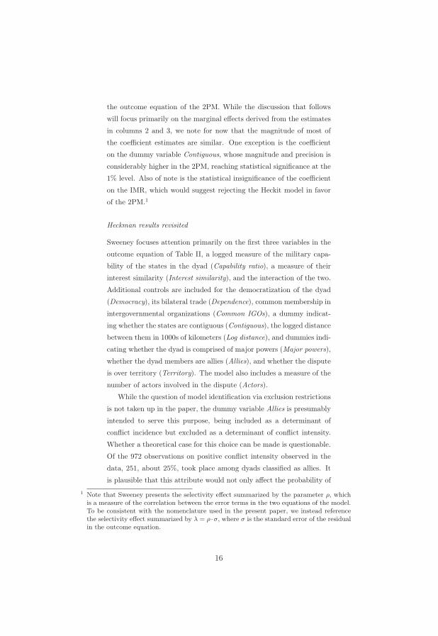
the outcome equation of the 2PM. While the discussion that follows
will focus primarily on the marginal effects derived from the estimates
in columns 2 and 3, we note for now that the magnitude of most of
the coefficient estimates are similar. One exception is the coefficient
on the dummy variable Contiguous, whose magnitude and precision is
considerably higher in the 2PM, reaching statistical significance at the
1% level. Also of note is the statistical insignificance of the coefficient
on the IMR, which would suggest rejecting the Heckit model in favor
of the 2PM.1
Heckman results revisited
Sweeney focuses attention primarily on the first three variables in the
outcome equation of Table II, a logged measure of the military capa-
bility of the states in the dyad (Capability ratio), a measure of their
interest similarity (Interest similarity), and the interaction of the two.
Additional controls are included for the democratization of the dyad
(Democracy), its bilateral trade (Dependence), common membership in
intergovernmental organizations (Common IGOs), a dummy indicat-
ing whether the states are contiguous (Contiguous), the logged distance
between them in 1000s of kilometers (Log distance), and dummies indi-
cating whether the dyad is comprised of major powers (Major powers),
whether the dyad members are allies (Allies), and whether the dispute
is over territory (Territory). The model also includes a measure of the
number of actors involved in the dispute (Actors).
While the question of model identification via exclusion restrictions
is not taken up in the paper, the dummy variable Allies is presumably
intended to serve this purpose, being included as a determinant of
conflict incidence but excluded as a determinant of conflict intensity.
Whether a theoretical case for this choice can be made is questionable.
Of the 972 observations on positive conflict intensity observed in the
data, 251, about 25%, took place among dyads classified as allies. It
is plausible that this attribute would not only affect the probability of
1 Note that Sweeney presents the selectivity effect summarized by the parameter ρ, which
is a measure of the correlation between the error terms in the two equations of the model.
To be consistent with the nomenclature used in the present paper, we instead reference
the selectivity effect summarized by λ = ρ ·σ, where σ is the standard error of the residual
in the outcome equation.
16

Table III: Mean Marginal Effect Estimates
Sweeney’s Calculations Authors’ Calculations Authors’ CalculationsMarg. Eff. Std. Dev. Marg. Eff. Std. Error Marg. Eff. Std. Error
Heckman Model Heckman Model Two-Part Model
Capability ratio 131.262 0.058 −13.092 12.833 −8.496∗∗ 2.311Democracy 0.474 0.003 0.474 0.310 −0.228∗∗ 0.049Dependence −1353.079 1.591 −1353.121∗∗ 289.236 −301.597∗∗ 53.081Common IGOs −0.143 0.001 −0.143 0.103 0.070∗∗ 0.017Contiguous 11.071 0.096 10.831∗∗ 3.816 7.849∗∗ 0.813Log distance −1.507 0.017 −0.855 1.007 −6.203∗∗ 1.313
∗ denotes significance at the 5%, ∗∗ at the 1% level. Marg. Eff. is for marginal effect, Std. Dev. isfor standard deviation, and Std. Error is for standard error.
conflict, but also its intensity, rendering it an inappropriate variable
for identifying the model.
Table III presents select marginal effects derived from the model.
Columns 1 and 2 presents Sweeney’s derivation of the mean marginal
effects averaged over the observations – all of which are calculated using
equation (5) – and their associated standard deviation, respectively.
Column 3 presents an updated calculation of the mean marginal effect
that takes into account the functional form of the explanatory variables
(continuous, dummy, logged, or interacted) and column 4 presents the
associated standard error, calculated using the delta method.
A comparison of columns 1 and 3 demonstrates that the adjustment
for functional form can matter. For the case of the dummy variable
Contiguous, the calculation of which in column 3 uses equation (8), the
difference between the estimates is rather moderate, but this is not so
for the logged and interacted variables. With respect to the variable
Log distance, for example, the estimate in column 1 suggests that a
one unit change in the logged value of distance is associated with a
1.5 reduction on the potential conflict intensity scale. To reinterpret
the impact of this variable as a marginal effect, that is, as the effect
of a 1000 kilometer increase in distance on potential conflict intensity,
requires the following equation, which accounts for the logged form of
the variable:
∂E[y|R∗ > 0]
∂xk
=βk
xk
− βλ
τk
xk
φ(xT1τ )
Φ(xT1τ )
[φ(xT
1τ )
Φ(xT1τ )
+ (xT1τ )
], (10)
where xk denotes distance measured in levels. This calculation yields a
17

considerably smaller mean estimate of -0.855, with the standard error,
calculated by the delta method, rendering it statistically insignificant.
The relatively high standard errors of many of the remaining marginal
effects in the Heckman model is a likely consequence of severe multi-
collinearity, an issue we return to Section 4.
An even sharper discrepancy is seen for the variable Capability ra-
tio, the variable of primary interest in the original study, which is
both logged and interacted with the variable Interest similarity in the
outcome equation. The marginal effect for this variable is given by:
∂E[y|R∗ > 0]
∂xk
=βk
xk
+βklxl
xk
−βλ
τk
xk
φ(xT1τ )
Φ(xT1τ )
[φ(xT
1τ )
Φ(xT1τ )
+(xT1τ )
], (11)
where xk denotes the Capability ratio measured in levels, xl is Interest
similarity, and βkl is the coefficient of the interaction of the Capability
ratio and Interest similarity. Contrasting markedly with the estimate
of 131.26 from the application of equation (5), equation (11) yields a
mean marginal effect of -13.09 with an associated standard error of
12.83.
Further insight into the effect of the Capability ratio can be gleaned
from plotting each observation-specific marginal effect against its as-
sociated z-statistic. The top panel of Figure 1 presents this plot for
the whole range of observations. Relatively few points fall outside the
absolute 1.96–threshold that indicates significance at the 5% level, and
all of these have a marginal effect less than or equal to -25. The major-
ity of marginal effects estimates – including all of those with a positive
sign – are statistically insignificant. The histogram in panel 2 facili-
tates a more transparent view of the distribution of marginal effects
that shows the density corresponding to each value; three peaks in the
density are visible at values of around -25, -8, and 0. This pattern high-
lights how in non-linear models the individual marginal effects can vary
significantly depending upon at what point in the data the effects are
calculated. Overall, the impression conveyed by Figure 1 is markedly
different from the seemingly tightly estimated mean of 131.26 (with a
standard deviation of 0.058) in column 1 of Table III.
In this regard, it bears noting that the standard deviations describ-
ing the spread of the marginal effects in column 2 are not remotely
18

Figure I: Marginal Effects of Capability ratio from the Heckman Model−2
−10
12
Z−S
tatis
tic
−60 −40 −20 0 20 40 60 80Marginal Effect
0.0
1.0
2.0
3.0
4D
ensi
ty
−60 −40 −20 0 20 40 60 80Marginal Effect
related to the statistical significance of these effects. Nor is it possible
to infer the significance level of the marginal effects by referencing the
coefficient estimates in Table III. For example, the coefficient of the
Contiguous dummy is statistically insignificant, leading Sweeney (p.
746) to discard its importance, even though its marginal effect is sig-
nificant at the 1% level. The opposite pattern is seen for the variable
Democracy; its coefficient is statistically significant at the 10% level
while the marginal effect is insignificant.
Two-part results
The final two columns of Table III present the marginal effects and
standard errors derived from the 2PM. The marginal effects of con-
tinuous level-variables and of dummies are derived from equations (7)
and (9), respectively. The formula for logged variables is given by
∂E[y]
∂xk
=βk
xk
Φ(xT1τ ) +
τk
xk
φ(xT1τ )(xT
2β) , (12)
19

If the logged variable is additionally interacted with a levels variable,
as in the case of the interaction of the Capability Ratio with Interest
Similarity, then the formula is given by:
∂E[y]
∂xk
=
[βk
xk
+βklxl
xk
]Φ(xT
1τ ) +
τk
xk
φ(xT1τ )(xT
2β) , (13)
Several notable differences are revealed by a comparison of the 2PM
and Heckman results, both with respect to the magnitude and sign of
the marginal effects as well as their statistical significance. For ex-
ample, while the magnitude of the mean estimate on the Capability
Ratio from the 2PM is, at -8.5, roughly 35% lower than that of the
Heckman model, its precision is considerably higher. Figure 2 plots
the observation-specific marginal effects against the Z-statistic. The
plot is limited to the 920 uncensored observations on warring dyads, in
line with the 2PM’s focus on actual outcomes. Statistically significant
results are obtained over most of the observations in the data. More-
over, with the exception of a single observation, all of the estimated
results fall below zero. Thus, contrasting with Sweeney (2003), this
finding lends support to the hypothesis that dyads characterized by a
preponderance of power of one of the states have less intense conflicts.
Two other contrasting results pertain to the variables Democracy
and Common IGOs. The marginal effects of these variables are posi-
tive and negative, respectively, in the Heckman model, though neither
is statistically significant. Conversely, they have the opposite signs
and are highly significant in the 2PM. Specifically, the results suggest
that each unit increase in the democracy index is associated with a 0.22
decrease in conflict intensity among warring dyads, providing some con-
firmation to the argument that democracies are more peaceful vis a vis
each other. By contrast, each unit increase in the index of membership
in intergovernmental organizations is associated with a 0.017 increase
in conflict intensity. While at first blush counter-intuitive, this may
reflect the tendency for states to seek membership in IGOs on the ba-
sis of interests for which they have a large stake, with a corresponding
willingness to wage war.
20

Figure II: Marginal Effects of Capability ratio from the 2PM−8
−6−4
−20
2Z−
Sta
tistic
−50 −45 −40 −35 −30 −25 −20 −15 −10 −5 0Marginal Effect
0.0
5.1
.15
Den
sity
−50 −45 −40 −35 −30 −25 −20 −15 −10 −5 0Marginal Effect
Which model to use?
The foregoing comparison brings into sharp relief why careful reflec-
tion surrounding selection of the appropriate model is warranted; the
results and conclusions drawn from the analysis may depend fundamen-
tally on this choice. Unfortunately, there are no hard and fast rules
that point to the superiority of one model over the other in any given
situation. As Madden (2008) has suggested, it therefore behooves re-
searchers to consider a combination of criteria – theoretical, practical,
and statistical – for guiding model selection.
With respect to theoretical considerations, the most important is-
sue to resolve is whether the goal of the study is to model potential or
actual outcomes, along with the related question of whether the cen-
sored observations on the dependent variable constitute missing values
or zeros. If the potential outcome is of interest, the choice is clear:
use the Heckman model, as potential outcomes cannot be derived from
21

the 2PM. To take one example that appears to be a warranted case
for employing the Heckman model, Martinez et al. (2008) undertake
am analysis that relates people’s socio-demographic attributes to their
estimates of the size of the gay population in Florida. Roughly 18% of
their sample responded “don’t know” when asked to give an estimate,
a response that clearly constitutes a missing value rather than a zero,
and one for which the notion of potential outcome is appropriate.
Nevertheless, we speculate that many political science applications
using data with a large share of zeros aim to model actual outcomes,
even when this objective is not stated explicitly. In one recent exam-
ple, Carson et al. (2011) estimate a Heckman model to analyze the
determinants of whether political challengers run for office in US Con-
gressional races and, given so, the share of the vote they win in the
election. The outcome equation of the model thus examines “election
results once experienced candidates have made their entry decisions.”
(p. 472) This phrasing, as well as the subsequent interpretation of the
results in terms of the challengers who actually run for office (at the
exclusion of those who might have run), suggests that the authors are
primarily concerned with the actual outcomes of elections rather than
the outcomes that might have occurred for those who did not run.
Presuming that the actual outcome is of interest, then the Heckman
model, coupled with Equation 6 to recover the corresponding marginal
effects, may still be the appropriate choice. Whether this is the case
will depend on additional statistical and practical considerations. The
balance would tilt toward application of a Heckman model if: (1) the
analyst has reservations about the 2PM’s assumption that the discrete
and continuous parts of the model are independent conditional on x
(which can be tested by reference to the coefficient on the inverse Mills
ratio), and (2) theoretically supported exclusion restrictions can be
identified for inclusion in the first stage probit. That this latter con-
sideration is repeatedly ignored is no doubt at least partly related to
the fact that such restrictions do not immediately avail themselves for
many questions of interest to political scientists. Unfortunately, there
are rarely easy fixes to this conundrum. Arbitrarily excluding variables
from the outcome equation is not a solution to the identification prob-
lem, nor is it legitimate to include irrelevant variables in the selection
equation (Heckman et al., 1999).
22

Even when theoretically supported exclusions restrictions can be
identified and a statistically significant coefficient on the inverse Mills
coefficient points to the application of a Heckman model, caution is
warranted. Wooldridge (2010) presents an example of an a Exponen-
tial Type II Tobit, of which the Heckit model is one variety, yielding
an implausibly signed yet highly significant estimate of the selectivity
parameter along with other difficult-to-interpret results, leading him
to conclude that the “model has some serious shortcomings even if we
accept the exclusion restrictions” (p. 702). Based on results from a
Monte Carlo example, Dow and Norton (2003) also urge caution. Their
simulations show that when there is a high degree of correlation be-
tween a coefficient and the inverse Mills coefficient, the magnitude of
the former may be unusually small and that of the latter unusually
high, biasing the results of a t-test on the inverse Mills ratio in favor
of the Heckman model in exactly those models in which the t-statistic
on a coefficient of interest is unusually small.
It is therefore imperative to undertake statistical diagnostic tests
to assess the extent to which multicollinearity may afflict the results.
One such diagnostic is afforded by the condition number, among several
suggested by Belsley (1991) for assessing the extent of multicollinearity.
This measure, which indicates how close a data matrix x is to being
singular, is computed from the eigenvalues of the moment matrix. A
higher condition number indicates a greater likelihood of collinearity
problems, whereby Belsey et al. (1980) suggest a maximum thresh-
old of 30 on the basis of Monte Carlo experiments. The condition
number obtained from the data analyzed here is 87, far exceeding this
threshold and suggesting that multicollinearity indeed poses a serious
problem when using the Heckman model to explain dispute severity.
This is perhaps not surprising given that a single dummy variable of
questionable theoretical validity, Allies, served to identify the model.
Beyond casting doubt on the estimates from a Heckman model,
such a high condition number, coupled with an interest in the actual
outcome, would clearly point in favor of a 2PM.
23

Conclusion
Censored data is a prevalent feature of political science research, one
that has been increasingly addressed by applying Heckman’s sample
selection model. The purpose of the present paper has been to cast
a critical light on how this empirical approach is commonly imple-
mented in the applied literature. Using the Heckman analysis of con-
flict intensity by Sweeney (2003), we pointed out several pitfalls in the
derivation of marginal effects and their statistical significance. Our
estimates, which took into account the functional form of the explana-
tory variable of interest, suggested fundamentally different conclusions
than those reached by Sweeney concerning the impact of key variables
in the model. Beyond this, we pursued the more basic issue of the
selection model’s applicability to the questions typically addressed by
political scientists, and suggested that a closely-related alternative, the
two-part model, may afford a more appropriate means for modeling the
data generation process.
Whether this is the case hinges on whether the aim of the analysis
is to model potential or actual outcomes. Potential outcomes are of
relevance when the modeler treats the censored values as unobserved
and wants to estimate the effect of an independent variable for both
these and the observed realizations of the dependent variable. Sample
selection bias may emerge in this case if there are unobserved variables
that determine both selection into the sample and the outcome vari-
able. To correct for this bias requires the specification of theoretically
supported exclusion restrictions in the selection equation of the model,
a critical step that is often disregarded in applied work.
When the aim is to instead model actual outcomes – that is, the
effect of an independent variable on positive values of the dependent
variable – sample selection bias is not of relevance because the censored
values of the dependent variable are observed and treated as zeros.
We believe this case is far more prevalent in political science data.
Various forms of foreign aid was cited as one of several examples of
a fully observed dependent variable for which the notion of missing
values is inappropriate: The absence of foreign aid plausibly represents
a case in which zero foreign aid is expended, just as the absence of
conflict, refugee flows, arms sales, or foreign direct investment plausibly
24

represents instances in which each of these dependent variables is zero.
This interpretation suggests the application of the two-part model.
One of the key practical advantages of the model is that no exclusion
restrictions are required for its identification, making it less sensitive
to specification errors.
Instances may nevertheless arise when the choice between the mod-
els is unclear. When this occurs, we would advocate estimating both
models to explore the extent to which the results diverge. If the di-
vergence is found to be substantial, then more exploration would be
required to identify the source of the discrepancy. At the least, such
a circumstance would dictate greater caution in drawing conclusions
from the analysis, including a careful appraisal of whether sample selec-
tivity poses a potential source of bias and if so, how it can be remedied
through the judicious selection of exclusion restrictions.
Replication Data
The data and annotated code for replicating the presented results,
written in Stata, has been uploaded to the journal’s web site (www.
prio.no/jpr/datasets).
Acknowledgements
The authors express their gratitude for the highly constructive com-
ments of four anonymous reviewers.
References
Baccini, L. (2010). Explaining formation and design of EU trade agree-
ments: The role of transparency and flexibility. European Union
Politics 11 (2), 195–217.
Belsey, D. A., E. Kuh, and R. E. Welsch (1980). Regression diagnostics:
Identifying influential data and sources of collinearity. John Wiley.
Belsley, D. (1991). Conditioning diagnostics - collinearity and weak
data. New York .
25

Blanton, S. L. (2005). Foreign policy in transition? Human rights,
democracy, and US arms exports. International Studies Quar-
terly 49 (4), 647–668.
Böhmelt, T. (2010). The effectiveness of tracks of diplomacy strategies
in third-party interventions. Journal of Peace Research 47 (2), 167–
178.
Brandt, P. T. and C. J. Schneider (2007). So the reviewer told you to
use a selection model? selection models and the study of interna-
tional relations. Working Paper .
Brulé, D. J., B. W. Marshall, and B. C. Prins (2010). Opportunities
and presidential uses of force a selection model of crisis decision-
making. Conflict Management and Peace Science 27 (5), 486–510.
Buhaug, H. (2010). Dude, where’s my conflict? LSG, relative strength,
and the location of civil war. Conflict Management and Peace Sci-
ence 27 (2), 107–128.
Carson, J. L., M. H. Crespin, C. P. Eaves, and E. Wanless (2011).
Constituency Congruency and Candidate Competition in US House
Elections. Legislative Studies Quarterly 36 (3), 461–482.
Chiricos, T. G. and W. D. Bales (1991). Unemployment and punish-
ment: an empirical assessment. Criminology 29 (4), 701–724.
Cragg, J. G. (1971). Some statistical models for limited dependent
variables with application to the demand for durable goods. Econo-
metrica, 829–844.
Diehl, P. F. and G. Goertz (2001). War and peace in international
rivalry. University of Michigan Press.
Dow, W. H. and E. C. Norton (2003). Choosing between and inter-
preting the Heckit and two-part models for corner solutions. Health
Services and Outcomes Research Methodology 4 (1), 5–18.
Drury, A. C., R. S. Olson, and D. A. V. Belle (2005). The politics of hu-
manitarian aid: US foreign disaster assistance, 1964–1995. Journal
of Politics 67 (2), 454–473.
26

Duan, N., W. G. Manning, C. N. Morris, and J. P. Newhouse (1984).
Choosing between the sample-selection model and the multi-part
model. Journal of Business & Economic Statistics 2 (3), 283–289.
Frondel, M. and C. J. Vance (2012). Interpreting the outcomes of
two-part models. Applied Economics Letters 19 (10), 987–992.
Gilardi, F. (2005). The formal independence of regulators: a com-
parison of 17 countries and 7 sectors. Swiss Political Science Re-
view 11 (4), 139–167.
Grier, K. B., M. C. Munger, and B. E. Roberts (1994). The determi-
nants of industry political activity, 1978-1986. American Political
Science Review , 911–926.
Hay, J. W., R. Leu, and P. Rohrer (1987). Ordinary Least Squares
and Sample-Selection Models of Health-Care Demand Monte Carlo
Comparison. Journal of Business & Economic Statistics 5 (4), 499–
506.
Heckman, J. J. (1979). Sample selection bias as a specification error.
Econometrica, 153–161.
Heckman, J. J., R. J. LaLonde, and J. A. Smith (1999). The economics
and econometrics of active labor market programs. Handbook of
labor economics 3, 1865–2097.
Henne, P. S. (2012). The two swords Religion–state connections and
interstate disputes. Journal of Peace Research 49 (6), 753–768.
Jensen, N. (2003). Democratic governance and multinational corpo-
rations: Political regimes and inflows of foreign direct investment.
International organization 57, 587–616.
Jeydel, A. and A. J. Taylor (2003). Are women legislators less effective?
Evidence from the US House in the 103rd-105th Congress. Political
Research Quarterly 56 (1), 19–27.
Karreth, J. and J. Tir (2013). International Institutions and Civil War
Prevention. The Journal of Politics 75 (01), 96–109.
27

Kingsnorth, R. F., R. C. MacIntosh, and S. Sutherland (2002). Crim-
inal charge or probation violation? Prosecutorial discretion and
implications for research in criminal court precessing. Criminol-
ogy 40 (3), 553–578.
Koch, M. and S. S. Gartner (2005). Casualties and Constituencies
Democratic Accountability, Electoral Institutions, and Costly Con-
flicts. Journal of Conflict Resolution 49 (6), 874–894.
Lebovic, J. H. (2004). Uniting for peace? Democracies and United
Nations peace operations after the Cold War. Journal of Conflict
Resolution 48 (6), 910–936.
Leung, S. F. and S. Yu (1996). On the choice between sample selection
and two-part models. Journal of Econometrics 72 (1), 197–229.
Lin, T.-F. and P. Schmidt (1984). A test of the Tobit specification
against an alternative suggested by Cragg. The Review of Economics
and Statistics, 174–177.
Macmillan, R. (2000). Adolescent Victimization and Income Deficits
in Adulthood: Rethinking the Costs of Criminal Violence from a
Life-Course Perspective. Criminology 38 (2), 553–588.
Maddala, G. S. (1992). Introduction to Econometrics. Macmillan Pub-
lishing Company New York.
Madden, D. (2008). Sample selection versus two-part models revis-
ited: The case of female smoking and drinking. Journal of Health
Economics 27 (2), 300–307.
Manning, W. G., N. Duan, and W. H. Rogers (1987). Monte carlo ev-
idence on the choice between sample selection and two-part models.
Journal of Econometrics 35 (1), 59–82.
Martinez, M. D., K. D. Wald, and S. C. Craig (2008). Homophobic
innumeracy? Estimating the size of the gay and lesbian population.
Public Opinion Quarterly 72 (4), 753–767.
Moffitt, R. A. (1999). New developments in econometric methods for
labor market analysis. Handbook of Labor Economics 3, 1367–1397.
28

Moore, W. H. and S. M. Shellman (2006). Refugee or internally dis-
placed person? To where should one flee? Comparative Political
Studies 39 (5), 599–622.
Peterson, T. M. and L. Graham (2011). Shared human rights norms
and military conflict. Journal of Conflict Resolution 55 (2), 248–273.
Poe, S. C. and J. Meernik (1995). US military aid in the 1980s: A
global analysis. Journal of Peace Research 32 (4), 399–411.
Puhani, P. (2000). The Heckman correction for sample selection and
its critique. Journal of Economic Surveys 14 (1), 53–68.
Sartori, A. E. (2003). An Estimator for Some Binary-Outcome Se-
lection Models Without Exclusion Restrictions. Political Analy-
sis 11 (2), 111–138.
Shrestha, M. K. and R. C. Feiock (2011). Transaction cost, exchange
embeddedness, and interlocal cooperation in local public goods sup-
ply. Political Research Quarterly 64 (3), 573–587.
Sigelman, L. and L. Zeng (1999). Analyzing censored and sample-
selected data with Tobit and Heckit models. Political Analysis 8 (2),
167–182.
Sweeney, K. J. (2003). The Severity of Interstate Disputes Are Dyadic
Capability Preponderances Really More Pacific? Journal of Conflict
Resolution 47 (6), 728–750.
Timpone, R. J. (1998). Structure, behavior, and voter turnout in the
United States. American Political Science Review , 145–158.
Vance, C. (2009). Marginal effects and significance testing with Heck-
man’s sample selection model: a methodological note. Applied Eco-
nomics Letters 16 (14), 1415–1419.
Wooldridge, J. M. (2010). Econometric Analysis of Cross Section and
Panel Data. The MIT Press.
29


