NGU Report 2008.050 Thermal diffusivity measurement at NGU

NGU Report 2008.050

Thermal diffusivity measurement at NGU – Status and method development 2005-2008

Geological Survey ofNorwayNO-7441 Trondheim, NorwayTel.: 47 73 904000Telefax 4773921620 REPORT

Report no.: 2008.050 ISSN 0800-3416 Grading: Open

Title:Thennal diffusivity measurement at NGU - Status and method development 2005-2008

Authors: Client:Randi Kalskin Ramstad, Hans de Beer, Kirsti NGU

Midttømme, Janusz Koziel and Bjørn WissingCounty: Commune:

Map-sheet name (M-l :250.000) Map-iheet no. and -name (M-I :50.000)

Deposit name and grid-reference: Number of pages: 41 Price (NOK): 240Map enclosures:

Fieldwork carried out: Date of report: Project no.: Person responsibl J20.05.2009 322600.Rh..L. ~-I: ~Æ

~=~~iPment fot measuring thermal diffusivity of rock samples is b';'ed on Middleton (1993). T~ermal condu tivity iscaleulated as a product of density (p), specific heat capacity (Cp) and thermal diffusivity (a). During the period from spring 2005to the present day, a series of tests and analyses has been performed to: (1) increase aur understanding of the thermal processesoccurring during testing, and (2) to improve NGU's routines and reproducibility. There still remains significant scope forimprovement.

Determination of the thermal properties of rock samples from Norwegian bedrock is not straightforward. The material isinhomogeneaus and anisotropic; properties may vary over a scale of centimetres and according to sample orientation. With this inmind, in order to obtain areasonable understanding of the thermal conductivity distribution, either at·depth in a cored borehole ornear the bedrock surface, the number of analysed samples is a critical factor. Thus, many samples with "adequate" analyticalquality might be preferable to relatively few samples analysed with high accuracy.

A number of individual improvements to the thermal diffusivity equipment at NGU have resulted in overall improvedreproducibility in measured values and better operational routines. Amongst these improvements, increased temperature of theheat source, more robust temperature sensors and the application of acceptance criteria are considered to be the three mostimportant. In addition, the use of a certified reference material, with a thermal diffusivity within the expected range of "real rock"values, has also contributed to overall quality assurance. The certification ofPyroceram at lRRM last year (Salmon et al., 2007),here called BCR-724, represented a breakthrough and ensures a proper quality contrai on all sample determinations with respectto both reproducibility and accuracy.

A ring test, involving the thermal conductivity labs at the University of Aarhus and at the Geological Survey of Finland (GTK)confirmed that NGU's determinations have satisfactory quality. All three laboratories returned some deviating results that, to alarge extent, can be related to the foliation and composition of the rock samples.

NGU's equipment for thermal diffusivity determination, and the subsequent calculation ofthermal conductivity, can be furtherimproved. In particular, the procedure for caleulating the thermal diffusivity from the temperature-time curve should be upgraded.FEFLOw"' modelling of the equipment setup and the dynamics of the thermal processes led to a better understanding andsuggested same further improvements.

From the start of2006 to May 2008, routine thermal diffusivity determinations have been carried out at NGU on approximately1000 core samples and 3000 snrface samples.

Keywords: Thermal conductivity Thennal diffusivity Laboratory equipment

Method development Modelling Pyroceram

BCR-724 Transient method Heat flow

CONTENTS

1. THEORETICAL BACKGROUND – MIDDLETON (1993) 6

2. EQUIPMENT, ROUTINES AND SOFTWARE DEVELOPMENT 9

2.1 Equipment 9 2.1.1 1998-version 9 2.1.2 2001-version 10 2.1.3 2006-version 11

2.2 Overview of the “Varmeled” software 13

3. QUALITY ASSURANCE AFTER 2005 – GENERAL IMPROVEMENTS 16

3.1 Reproducibility 16 3.1.1 Temporal variation in thermal conductivity of the reference material 18 3.1.2 Is thermal conductivity of the reference material dependent on resting time? 19 3.1.3 Need for a correction factor? 20 3.1.4 Testing variations of insulation material 22 3.1.5 Test of new heat sources 24

3.2 Regular measurements - working with improved equipment and routines 26

3.3 Thermophysical properties of Pyroceram. What are the correct values? 26

3.4 Ring test of thermal conductivity 30

3.5 Linear segment of the temperature-time curve? 34

3.6 Modelling of the apparatus and the dynamics during a measurement 35

4. DISCUSSION 37

5. CONCLUSIONS 39

6. REFERENCES 41

FIGURES Figure 1 A semi-infinite slab that is initially at zero temperature, insulated at the surface x = 0, and has a constant heat flux introduced at the surface x = a at time t = 0. Based on Middleton (1993). ............................... 7 Figure 2 Results of the experiment predicted by the theory in Equation 3, and the graphical meaning of ti, Ti and m from Equation 5 (based on Middleton, 1993). .................................................................................................... 8 Figure 3 First version of equipment for measuring thermal conductivity of rock samples at NGU, developed in 1998 (Midttømme et al., 2000). ............................................................................................................................... 9 Figure 4 The 2001-version of the laboratory equipment for thermal diffusivity measurements where a flat iron is the heat source. ..................................................................................................................................................... 10 Figure 5 New sample box with standard sized samples (left), although different diameters and shapes can also be accommodated (right). ..................................................................................................................................... 11 Figure 6 A disc-shaped plate of aluminium is fastened to the base of the flat iron to ensure a uniform surface temperature on the plate. ...................................................................................................................................... 11 Figure 7 New heat source, a black hotplate, with a temperature of 300°C ± 1°C. ............................................... 12 Figure 8 Coiled wire heat source. ......................................................................................................................... 12 Figure 9 Left: Sensor with thick copper signal wires and sample box made for one sample only. Middle: Sensors used in early 2006 without a thin pad of rubber foam. Right: Newest sensors equipped with thin wires of copper, a thin layer of foam and aluminium foil. ............................................................................................................... 13 Figure 10 Screen picture of the Sample database-part of the software where all the rock sample data are organized............................................................................................................................................................... 14 Figure 11 Temperature-time curve for four samples in the Measurements module. ............................................ 15 Figure 12 The calculation part of the software is divided into steps which lead to the final values of thermal diffusivity and thermal conductivity of the rock samples. ..................................................................................... 15 Figure 13 Thermal conductivity of six samples (kal_20 to kal_26) of the reference material Pyroceram made on the 2001-version of the NGU equipment, during routine determinations of rock samples of the Lito batch 2 sample set in June 2005. In each boxplot, the horizontal line within the box shows the median of the measurement series, the shaded box shows the interquartile range, the whiskers show the non-outlying extraquartile range, while crosses mark outlying data points. ............................................................................. 17 Figure 14 Temperature – time curves for the reference sample kal_22, where the calculated thermal conductivity varies in the range 3.6 to 4.4 W/m⋅K. .................................................................................................................... 18 Figure 15 Daily variability of determined thermal conductivity of the reference material Pyroceram, subdivided according to date of measurement and number of measurements (%) outside 3.9±10% W/m·K.......................... 19 Figure 16 Calculated thermal conductivity of the reference material plotted against resting time, i.e. the time between two sets of measurements. The left hand diagram shows all data, the right hand diagram shows only resting times up to 6 hours. ................................................................................................................................... 20 Figure 17 Thermal conductivity of 30 rock samples (Lito batch 2). The samples are measured five times each. 22 Figure 18 The different insulation plates used in the study (top row, plate A, C, G”; bottom row, plate H, I). Small variations in the material and layout of the plate should (in theory) not influence the determined thermal conductivity of the reference material. .................................................................................................................. 23 Figure 19 Thermal conductivity of the reference material using variants of polystyrene as insulation material. 24 Figure 20 Results from standard series of determinations on reference material, using four different experimental setups, employing different heat sources and sensor ages. On the left, the series are divided into individual cell positions. On the right, the results from different cells are aggregated. ....................................... 25 Figure 21 Histograms comparing the determined thermal conductivity values for the Lito B2-rock samples, measured with the use of different heat sources. ................................................................................................... 25 Figure 22 Thermal conductivity and thermal diffusivity of the certified BCR-724 (Pyroceram) for temperature between 20 and 50°C (based on Salmon et al., 2007). Thermal conductivity is plotted as a function of temperature (Equation 9) or calculated as a product of density (ρ), specific heat capacity (Cp) and thermal diffusivity (α). Results from NGU’s measured values of thermal diffusivity are plotted as a box-plot. Some selected values of specific heat capacity, from Equation 11, are listed to the right. ............................................. 29 Figure 23 Results from standard series of Pyroceram/BCR-724: similar to Figure 20 but here presented as thermal diffusivity rather than thermal conductivity. ............................................................................................ 30 Figure 24 Remnant Pyroceram material held by NGU......................................................................................... 30 Figure 25 Photographs of the rock samples in the ring test measured at NGU. .................................................. 32 Figure 26 A ring test of selected rock samples from different locations in Norway, where the University of Aarhus, the Geological Survey of Finland (GTK) and NGU participated. ........................................................... 33 Figure 27 Analysis of temperature-time data from a specific test (using the flat iron equipment) implies that the linearity of the temperature-time curve is not perfect and that temperature data collection routines could be improved. .............................................................................................................................................................. 34

TABLES Table 1 Mileposts in thermal conductivity testing since 2005. ............................................................................. 16 Table 2 Description of polystyrene plate used as insulation around the samples of reference material. ............. 22 Table 3 Lab-contracts performed with the improved routines and carried out in the period from the beginning of 2006 up to May 2008. ........................................................................................................................................... 26

INTRODUCTION A transient method for measuring thermal conductivity of rock samples has been developed at NGU since 1998. The method is mainly based on Middleton (1993). This report summarizes the different stages in the development of the thermal conductivity apparatus, with particular focus on the years 2005-2008. Some results from previous years have been reported in Midttømme et al. (2000 and 2004).

1. Theoretical background – Middleton (1993)

This chapter is mainly based on Middleton (1993). The thermal conductivity of rocks is calculated from thermal diffusivity (α) by using equation 1.

αρ pCK =

Equation 1

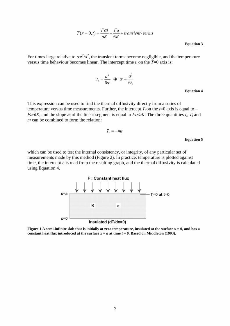
where K = Thermal conductivity (W/m·K) ρ = Density (kg/m3) Cp = Specific heat capacity (J/kg·K), and α = Thermal diffusivity (m2/s) The top of a rock sample is exposed to a heat flow which is assumed to be constant (at least, within the temperature range under which the measurements were taken). The heat flow is generated by a source which is controlled by a thermostat and which has a constant (high) temperature. The source is placed approximately 10 mm above the top surface of the sample during the measurements. The sample is insulated on all other surfaces. Temperature is measured at the base of the sample. Thermal diffusivity (α) is estimated from a plot of temperature versus time and the thermal conductivity (K) is calculated from Equation 1. The theory behind the method used in the development of the NGU-apparatus is based on a one-dimensional single-slab case, originally described by Carslaw and Jaeger (1959), and cited by Middleton (1993). They consider a semi-infinite slab that is initially at zero temperature, insulated at the surface x = 0, and that has a constant heat flux introduced at the surface x=a at time t=0 (Figure 1). Carslaw and Jaeger (1959) in Middleton (1993) showed that the temperature at a distance x within the slab at a time t, after introduction of a constant heat flux (F) on the top (x=a) of the slab, is given by:

⎟⎟⎠

⎞⎜⎜⎝

⎛ −−

−+= ∑∞

=−

1/

222

22

cos)1(26

3),(222

natn

n

axne

naax

KFa

aKtFtxT π

πα πα

Equation 2

where α is thermal diffusivity, K is thermal conductivity, and a is the thickness of the slab. If the temperature is measured at the base of the slab (x=0), the expression for the temperature becomes:

6

termstransientK

FaaK

tFtxT ⋅+−==6

),0( α

Equation 3

For times large relative to απ2/a2, the transient terms become negligible, and the temperature versus time behaviour becomes linear. The intercept time ti on the T=0 axis is:

α6

2ati = it

a6

2

=α

Equation 4

This expression can be used to find the thermal diffusivity directly from a series of temperature versus time measurements. Further, the intercept Ti on the t=0 axis is equal to –Fa/6K, and the slope m of the linear segment is equal to Fα/aK. The three quantities ti, Ti and m can be combined to form the relation:

ii mtT −=

Equation 5

which can be used to test the internal consistency, or integrity, of any particular set of measurements made by this method (Figure 2). In practice, temperature is plotted against time, the intercept ti is read from the resulting graph, and the thermal diffusivity is calculated using Equation 4.

Figure 1 A semi-infinite slab that is initially at zero temperature, insulated at the surface x = 0, and has a constant heat flux introduced at the surface x = a at time t = 0. Based on Middleton (1993).

7

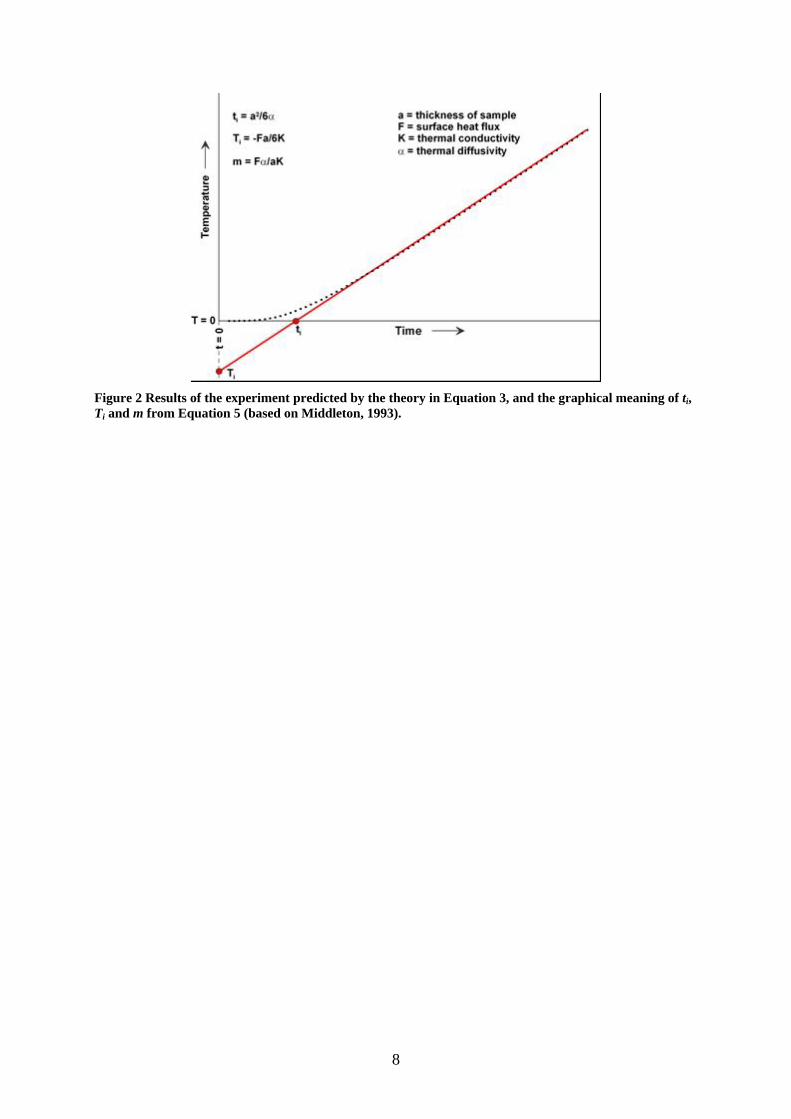
Figure 2 Results of the experiment predicted by the theory in Equation 3, and the graphical meaning of ti, Ti and m from Equation 5 (based on Middleton, 1993).

8

2. Equipment, routines and software development

2.1 Equipment The laboratory equipment for measuring the thermal diffusivity of rock samples at NGU has been modified several times since it was developed in 1998. For practical reasons, the different stages can be described in terms of three versions, with respect to the original equipment described in Middleton (1993).

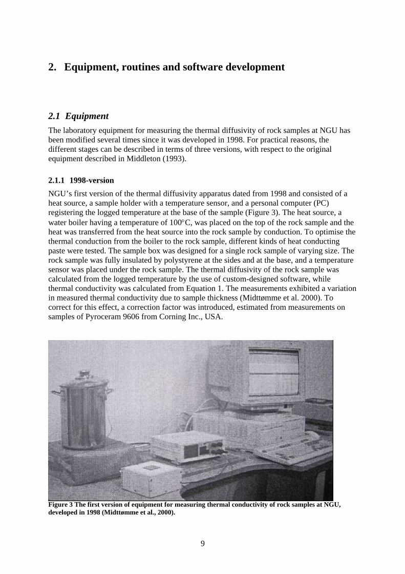
2.1.1 1998-version NGU’s first version of the thermal diffusivity apparatus dated from 1998 and consisted of a heat source, a sample holder with a temperature sensor, and a personal computer (PC) registering the logged temperature at the base of the sample (Figure 3). The heat source, a water boiler having a temperature of 100°C, was placed on the top of the rock sample and the heat was transferred from the heat source into the rock sample by conduction. To optimise the thermal conduction from the boiler to the rock sample, different kinds of heat conducting paste were tested. The sample box was designed for a single rock sample of varying size. The rock sample was fully insulated by polystyrene at the sides and at the base, and a temperature sensor was placed under the rock sample. The thermal diffusivity of the rock sample was calculated from the logged temperature by the use of custom-designed software, while thermal conductivity was calculated from Equation 1. The measurements exhibited a variation in measured thermal conductivity due to sample thickness (Midttømme et al. 2000). To correct for this effect, a correction factor was introduced, estimated from measurements on samples of Pyroceram 9606 from Corning Inc., USA.

Figure 3 The first version of equipment for measuring thermal conductivity of rock samples at NGU, developed in 1998 (Midttømme et al., 2000).

9

2.1.2 2001-version Since 1998, several modifications have been made to the laboratory equipment for thermal conductivity determination, including the following: • The heat transfer mechanism from the heat source to the top of the rock sample has been

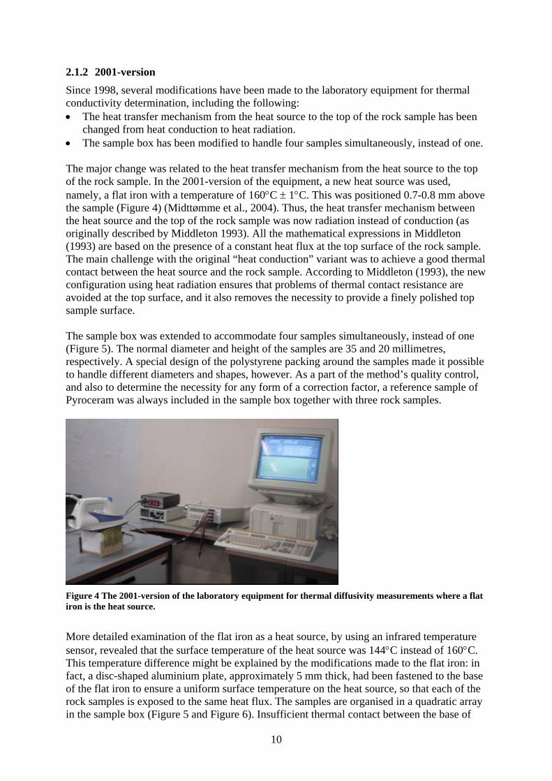
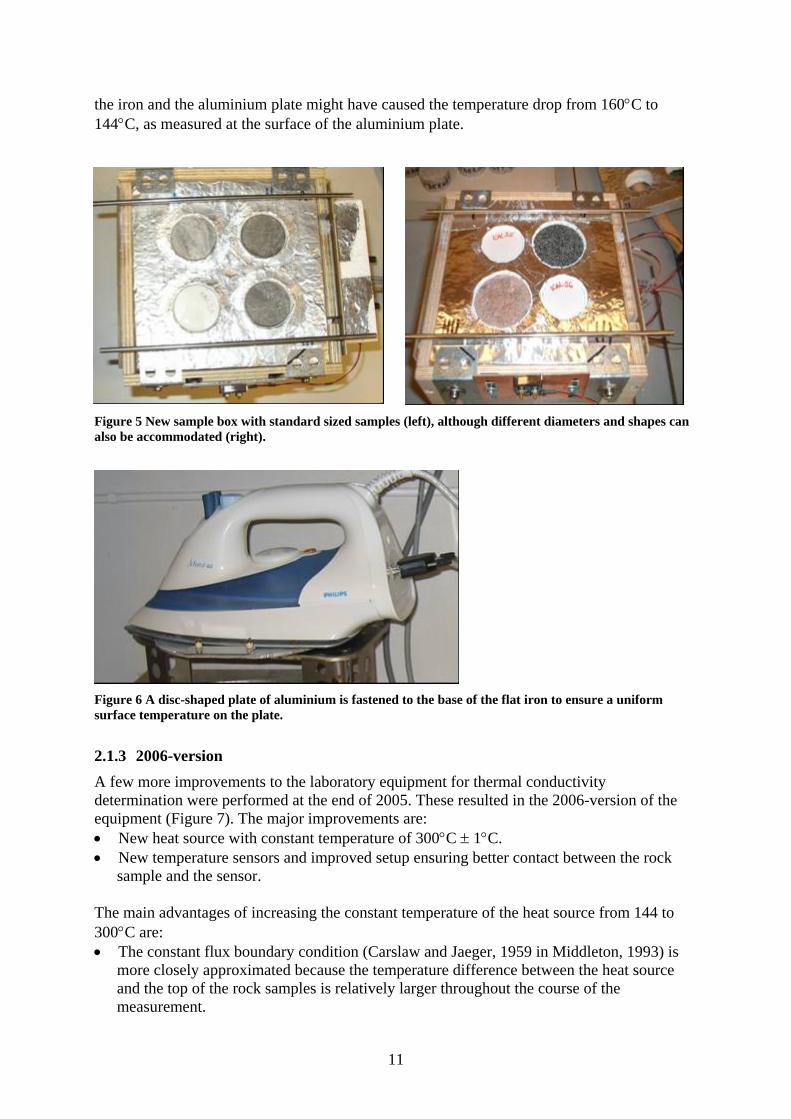
changed from heat conduction to heat radiation. • The sample box has been modified to handle four samples simultaneously, instead of one. The major change was related to the heat transfer mechanism from the heat source to the top of the rock sample. In the 2001-version of the equipment, a new heat source was used, namely, a flat iron with a temperature of 160°C ± 1°C. This was positioned 0.7-0.8 mm above the sample (Figure 4) (Midttømme et al., 2004). Thus, the heat transfer mechanism between the heat source and the top of the rock sample was now radiation instead of conduction (as originally described by Middleton 1993). All the mathematical expressions in Middleton (1993) are based on the presence of a constant heat flux at the top surface of the rock sample. The main challenge with the original “heat conduction” variant was to achieve a good thermal contact between the heat source and the rock sample. According to Middleton (1993), the new configuration using heat radiation ensures that problems of thermal contact resistance are avoided at the top surface, and it also removes the necessity to provide a finely polished top sample surface. The sample box was extended to accommodate four samples simultaneously, instead of one (Figure 5). The normal diameter and height of the samples are 35 and 20 millimetres, respectively. A special design of the polystyrene packing around the samples made it possible to handle different diameters and shapes, however. As a part of the method’s quality control, and also to determine the necessity for any form of a correction factor, a reference sample of Pyroceram was always included in the sample box together with three rock samples.

Figure 4 The 2001-version of the laboratory equipment for thermal diffusivity measurements where a flat iron is the heat source.

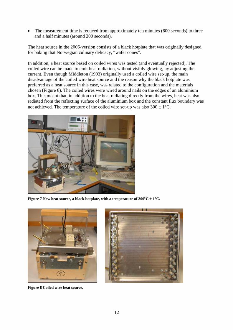
More detailed examination of the flat iron as a heat source, by using an infrared temperature sensor, revealed that the surface temperature of the heat source was 144°C instead of 160°C. This temperature difference might be explained by the modifications made to the flat iron: in fact, a disc-shaped aluminium plate, approximately 5 mm thick, had been fastened to the base of the flat iron to ensure a uniform surface temperature on the heat source, so that each of the rock samples is exposed to the same heat flux. The samples are organised in a quadratic array in the sample box (Figure 5 and Figure 6). Insufficient thermal contact between the base of

10

the iron and the aluminium plate might have caused the temperature drop from 160°C to 144°C, as measured at the surface of the aluminium plate.

Figure 5 New sample box with standard sized samples (left), although different diameters and shapes can also be accommodated (right).

Figure 6 A disc-shaped plate of aluminium is fastened to the base of the flat iron to ensure a uniform surface temperature on the plate.

2.1.3 2006-version A few more improvements to the laboratory equipment for thermal conductivity determination were performed at the end of 2005. These resulted in the 2006-version of the equipment (Figure 7). The major improvements are: • New heat source with constant temperature of 300°C ± 1°C. • New temperature sensors and improved setup ensuring better contact between the rock

sample and the sensor. The main advantages of increasing the constant temperature of the heat source from 144 to 300°C are: • The constant flux boundary condition (Carslaw and Jaeger, 1959 in Middleton, 1993) is

more closely approximated because the temperature difference between the heat source and the top of the rock samples is relatively larger throughout the course of the measurement.

11

• The measurement time is reduced from approximately ten minutes (600 seconds) to three and a half minutes (around 200 seconds).

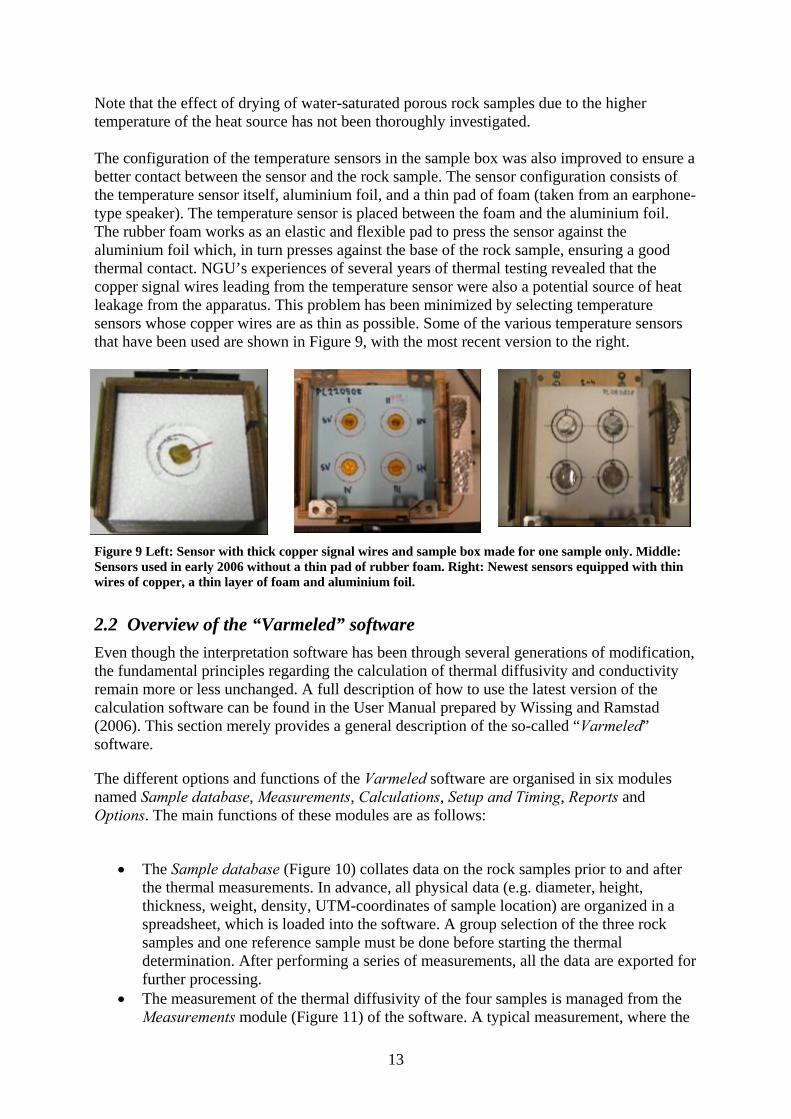
The heat source in the 2006-version consists of a black hotplate that was originally designed for baking that Norwegian culinary delicacy, “wafer cones”. In addition, a heat source based on coiled wires was tested (and eventually rejected). The coiled wire can be made to emit heat radiation, without visibly glowing, by adjusting the current. Even though Middleton (1993) originally used a coiled wire set-up, the main disadvantage of the coiled wire heat source and the reason why the black hotplate was preferred as a heat source in this case, was related to the configuration and the materials chosen (Figure 8). The coiled wires were wired around nails on the edges of an aluminium box. This meant that, in addition to the heat radiating directly from the wires, heat was also radiated from the reflecting surface of the aluminium box and the constant flux boundary was not achieved. The temperature of the coiled wire set-up was also 300 ± 1°C.

Figure 7 New heat source, a black hotplate, with a temperature of 300°C ± 1°C.

Figure 8 Coiled wire heat source.

12

Note that the effect of drying of water-saturated porous rock samples due to the higher temperature of the heat source has not been thoroughly investigated. The configuration of the temperature sensors in the sample box was also improved to ensure a better contact between the sensor and the rock sample. The sensor configuration consists of the temperature sensor itself, aluminium foil, and a thin pad of foam (taken from an earphone-type speaker). The temperature sensor is placed between the foam and the aluminium foil. The rubber foam works as an elastic and flexible pad to press the sensor against the aluminium foil which, in turn presses against the base of the rock sample, ensuring a good thermal contact. NGU’s experiences of several years of thermal testing revealed that the copper signal wires leading from the temperature sensor were also a potential source of heat leakage from the apparatus. This problem has been minimized by selecting temperature sensors whose copper wires are as thin as possible. Some of the various temperature sensors that have been used are shown in Figure 9, with the most recent version to the right.

Figure 9 Left: Sensor with thick copper signal wires and sample box made for one sample only. Middle: Sensors used in early 2006 without a thin pad of rubber foam. Right: Newest sensors equipped with thin wires of copper, a thin layer of foam and aluminium foil.

2.2 Overview of the “Varmeled” software Even though the interpretation software has been through several generations of modification, the fundamental principles regarding the calculation of thermal diffusivity and conductivity remain more or less unchanged. A full description of how to use the latest version of the calculation software can be found in the User Manual prepared by Wissing and Ramstad (2006). This section merely provides a general description of the so-called “Varmeled” software.

The different options and functions of the Varmeled software are organised in six modules named Sample database, Measurements, Calculations, Setup and Timing, Reports and Options. The main functions of these modules are as follows:

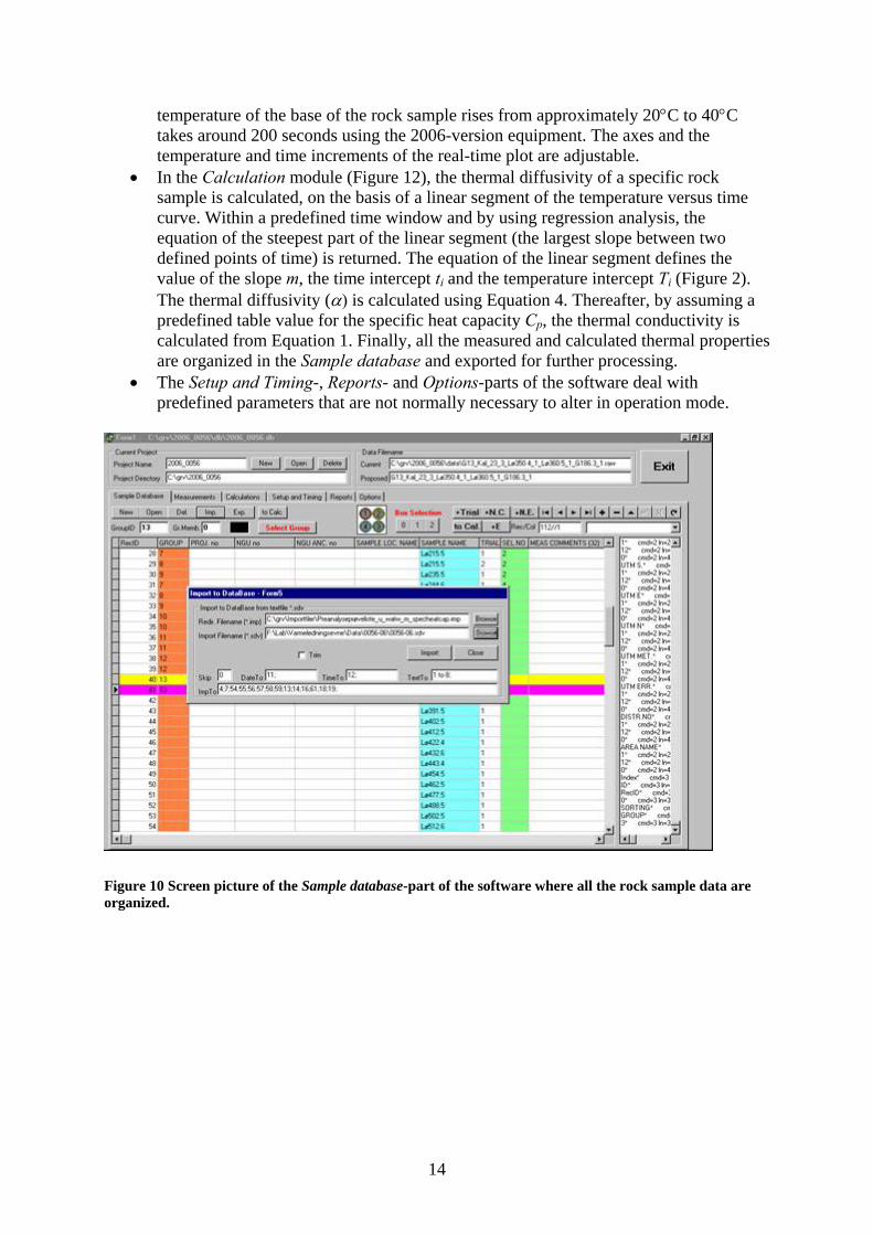
• The Sample database (Figure 10) collates data on the rock samples prior to and after

the thermal measurements. In advance, all physical data (e.g. diameter, height, thickness, weight, density, UTM-coordinates of sample location) are organized in a spreadsheet, which is loaded into the software. A group selection of the three rock samples and one reference sample must be done before starting the thermal determination. After performing a series of measurements, all the data are exported for further processing.

• The measurement of the thermal diffusivity of the four samples is managed from the Measurements module (Figure 11) of the software. A typical measurement, where the

13

temperature of the base of the rock sample rises from approximately 20°C to 40takes around 200 seconds using the 2006-version equipment. The axe

°C s and the

time

a

l properties

predefined parameters that are not normally necessary to alter in operation mode.

reen picture of the Sample database-part of the software where all the rock sample data are rganized.

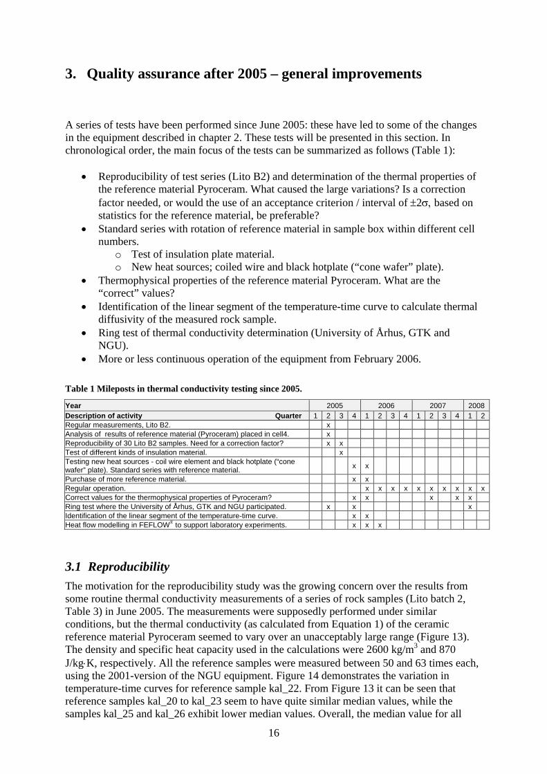
temperature and time increments of the real-time plot are adjustable. • In the Calculation module (Figure 12), the thermal diffusivity of a specific rock

sample is calculated, on the basis of a linear segment of the temperature versuscurve. Within a predefined time window and by using regression analysis, the equation of the steepest part of the linear segment (the largest slope between two defined points of time) is returned. The equation of the linear segment defines the value of the slope m, the time intercept ti and the temperature intercept Ti (Figure 2). The thermal diffusivity (α) is calculated using Equation 4. Thereafter, by assuming predefined table value for the specific heat capacity Cp, the thermal conductivity is calculated from Equation 1. Finally, all the measured and calculated thermaare organized in the Sample database and exported for further processing.

• The Setup and Timing-, Reports- and Options-parts of the software deal with

Figure 10 Sco

14

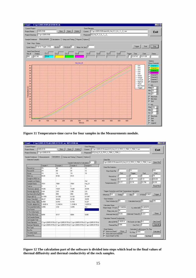
Figure 11 Temperature-time curve for four samples in the Measurements module.

Figure th

12 The calculation part of the software is divided into steps which lead to the final values of ermal diffusivity and thermal conductivity of the rock samples.

15

3. Quality assurance after 2005 – general improvements

A series of tests have been performed since June 2005: these have led to some of the changes in the equipment described in chapter 2. These tests will be presented in this section. In chronological order, the main focus of the tests can be summarized as follows (Table 1):

es of n

factor needed, or would the use of an acceptance criterion / interval of ±2σ, based on

l

sical properties of the reference material Pyroceram. What are the

ermal

l conductivity determination (University of Århus, GTK and

quipment from February 2006.

• Reproducibility of test series (Lito B2) and determination of the thermal properti

the reference material Pyroceram. What caused the large variations? Is a correctio

statistics for the reference material, be preferable? • Standard series with rotation of reference material in sample box within different cel

numbers. o Test of insulation plate material. o New heat sources; coiled wire and black hotplate (“cone wafer” plate).

• Thermophy“correct” values?

• Identification of the linear segment of the temperature-time curve to calculate thdiffusivity of the measured rock sample.

• Ring test of thermaNGU).

• More or less continuous operation of the e

1Table in thermal conductivity testing since 2005. Mileposts

2005 2006 Year 2007 2008 Description of activity Quarter 1 2 3 4 1 2 3 4 1 2 3 4 1 2 Regular measurements, Lito B2. x Analysis of results of reference material (Pyroceram) placed in cell4. x Reproducibility of 30 Lito B2 samples. Need for a correction factor? x x Test of different kinds of insulation material. x Testing new heat sources - coil wire element and black hotplate (“cone wafer” plate). Standard series with reference material. x x

Purchase of more reference material. x x Regular operation. x x x x x x x x x x Correct values for the thermophysical properties of Pyroceram? x x x x x Ring test where the University of Århus, GTK and NGU participated. x x x Identification of the linear segment of the temperature-time curve. x x Heat flow modelling in FEFLOW® to support laboratory experiments. x x x

3.1 Reproducibility The motivation for the reproducibility study was the growing concern over the results from

ductivity measurements of a series of rock samples (Lito batch 2, e measurements were supposedly performed under similar

70 each,

ll

some routine thermal conTable 3) in June 2005. Thconditions, but the thermal conductivity (as calculated from Equation 1) of the ceramic reference material Pyroceram seemed to vary over an unacceptably large range (Figure 13). The density and specific heat capacity used in the calculations were 2600 kg/m3 and 8J/kg⋅K, respectively. All the reference samples were measured between 50 and 63 times using the 2001-version of the NGU equipment. Figure 14 demonstrates the variation in temperature-time curves for reference sample kal_22. From Figure 13 it can be seen that reference samples kal_20 to kal_23 seem to have quite similar median values, while the samples kal_25 and kal_26 exhibit lower median values. Overall, the median value for a

16

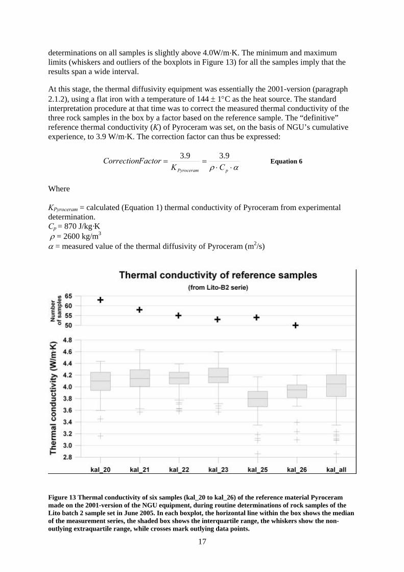
determinations on all samples is slightly above 4.0W/m·K. The minimum and maximum limits (whiskers and outliers of the boxplots in Figure 13) for all the samples imply that tresults span a wide interval.

At this stage, the thermal diffusivity equipment was essentially the 2001-version (paragraph

he

temperature of 144 ± 1°C as the heat source. The standard interpretation procedure at that time was to correct the measured thermal conductivity of the

ve

2.1.2), using a flat iron with a

three rock samples in the box by a factor based on the reference sample. The “definitive” reference thermal conductivity (K) of Pyroceram was set, on the basis of NGU’s cumulatiexperience, to 3.9 W/m·K. The correction factor can thus be expressed:

αρ ⋅⋅==

pPyroceram CKFactorCorrection 9.39.3 Equation 6

Where

Pyroceram = calculated (Equation 1) thermal conductivity of Pyroceram from experimental ation.

p = 870 J/kg·K

alue of the thermal diffusivity of Pyroceram (m2/s)

ade on the 2001-version of the NGU equipment, during routine determinations of rock samples of the ito batch 2 sample set in June 2005. In each boxplot, the horizontal line within the box shows the median f the measurement series, the shaded box shows the interquartile range, the whiskers show the non-

outlying extraquartile range, while crosses mark outlying data points.

KdeterminC ρ = 2600 kg/m3 α = measured v

Figure 13 Thermal conductivity of six samples (kal_20 to kal_26) of the reference material Pyroceram mLo

17

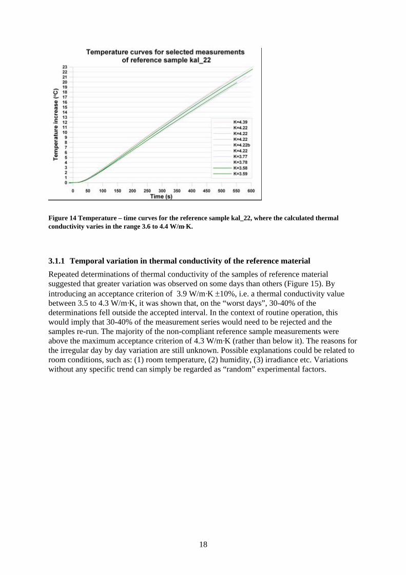
where the calculated thermal

.1.1 Temporal variation in thermal conductivity of the reference material

on some days than others (Figure 15). By troducing an acceptance criterion of 3.9 W/m·K ±10%, i.e. a thermal conductivity value

between 3.5 to 4.3 W/m·K, it was shown that, on the “worst days”, 30-40% of the n, this

ns for

to ariations

Figure 14 Temperature – time curves for the reference sample kal_22, conductivity varies in the range 3.6 to 4.4 W/m⋅K.

3Repeated determinations of thermal conductivity of the samples of reference material suggested that greater variation was observedin

determinations fell outside the accepted interval. In the context of routine operatiowould imply that 30-40% of the measurement series would need to be rejected and the samples re-run. The majority of the non-compliant reference sample measurements wereabove the maximum acceptance criterion of 4.3 W/m·K (rather than below it). The reasothe irregular day by day variation are still unknown. Possible explanations could be related room conditions, such as: (1) room temperature, (2) humidity, (3) irradiance etc. Vwithout any specific trend can simply be regarded as “random” experimental factors.

18

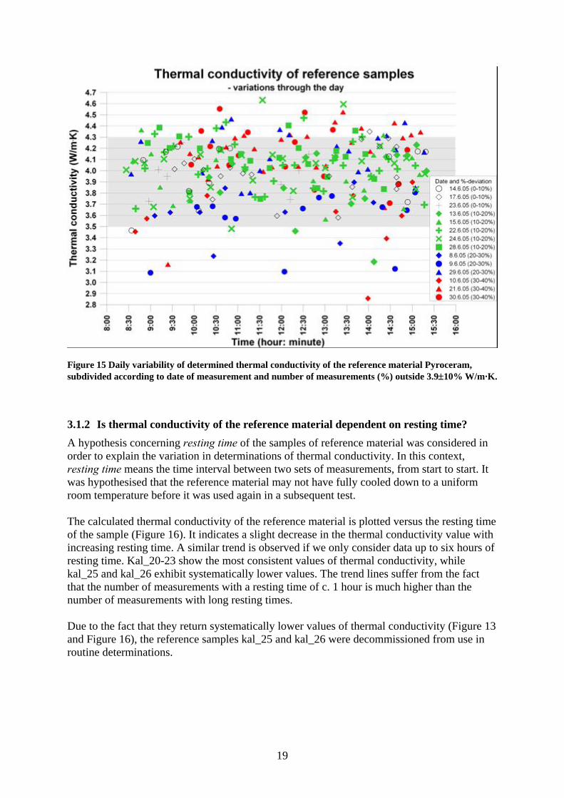
Figure 15 Daily variability of determined thermal conductivity of the reference material Pyroceram, bdivided according to date of measurement and number of measurements (%) outside 3.9±10% W/m·K.

.1.2 Is thermal conductivity of the reference material dependent on resting time?

lotted versus the resting time f the sample (Figure 16). It indicates a slight decrease in the thermal conductivity value with

r values of thermal conductivity (Figure 13 nd Figure 16), the reference samples kal_25 and kal_26 were decommissioned from use in

su

3A hypothesis concerning resting time of the samples of reference material was considered in order to explain the variation in determinations of thermal conductivity. In this context, resting time means the time interval between two sets of measurements, from start to start. It was hypothesised that the reference material may not have fully cooled down to a uniformroom temperature before it was used again in a subsequent test. The calculated thermal conductivity of the reference material is poincreasing resting time. A similar trend is observed if we only consider data up to six hours of resting time. Kal_20-23 show the most consistent values of thermal conductivity, while kal_25 and kal_26 exhibit systematically lower values. The trend lines suffer from the fact that the number of measurements with a resting time of c. 1 hour is much higher than thenumber of measurements with long resting times. Due to the fact that they return systematically lowearoutine determinations.

19

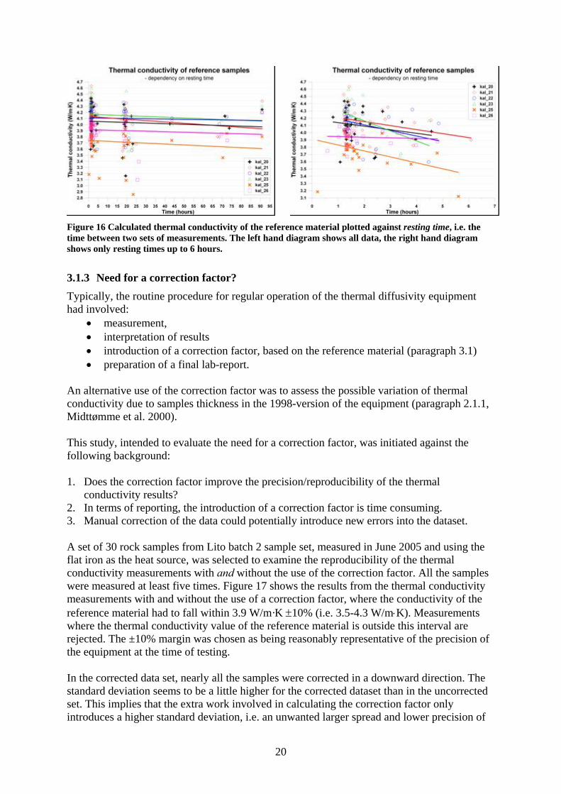
Figure 16 Calculated thermal conductivity of the reference material plotted against resting time, i.e. the time between two sets of measurements. The left hand diagram shows all data, the right hand diagram shows only resting times up to 6 hours.

3.1.3 Need for a correction factor? Typically, the routine procedure for regular operation of the thermal diffusivity equipment had involved:

• measurement, • interpretation of results • introduction of a correction factor, based on the reference material (paragraph 3.1) • preparation of a final lab-report.

An alternative use of the correction factor was to assess the possible variation of thermal conductivity due to samples thickness in the 1998-version of the equipment (paragraph 2.1.1, Midttømme et al. 2000). This study, intended to evaluate the need for a correction factor, was initiated against the following background: 1. Does the correction factor improve the precision/reproducibility of the thermal

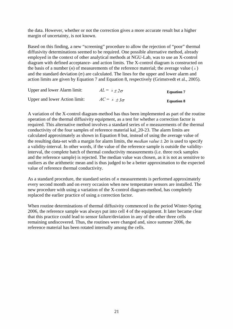
conductivity results? 2. In terms of reporting, the introduction of a correction factor is time consuming. 3. Manual correction of the data could potentially introduce new errors into the dataset. A set of 30 rock samples from Lito batch 2 sample set, measured in June 2005 and using the flat iron as the heat source, was selected to examine the reproducibility of the thermal conductivity measurements with and without the use of the correction factor. All the samples were measured at least five times. Figure 17 shows the results from the thermal conductivity measurements with and without the use of a correction factor, where the conductivity of the reference material had to fall within 3.9 W/m·K ±10% (i.e. 3.5-4.3 W/m⋅K). Measurements where the thermal conductivity value of the reference material is outside this interval are rejected. The ±10% margin was chosen as being reasonably representative of the precision of the equipment at the time of testing. In the corrected data set, nearly all the samples were corrected in a downward direction. The standard deviation seems to be a little higher for the corrected dataset than in the uncorrected set. This implies that the extra work involved in calculating the correction factor only introduces a higher standard deviation, i.e. an unwanted larger spread and lower precision of

20

the data. However, whether or not the correction gives a more accurate result but a higher margin of uncertainty, is not known. Based on this finding, a new “screening” procedure to allow the rejection of “poor” thermal diffusivity determinations seemed to be required. One possible alternative method, already employed in the context of other analytical methods at NGU-Lab, was to use an X-control diagram with defined acceptance- and action limits. The X-control diagram is constructed on the basis of a number (n) of measurements of the reference material; the average value ( x ) and the standard deviation (σ) are calculated. The lines for the upper and lower alarm and action limits are given by Equation 7 and Equation 8, respectively (Grimstvedt et al., 2005). Upper and lower Alarm limit: AL = x ± 2σ Equation 7

Upper and lower Action limit: AC = x ± 3σ Equation 8

A variation of the X-control diagram-method has thus been implemented as part of the routine operation of the thermal diffusivity equipment, as a test for whether a correction factor is required. This alternative method involves a standard series of n measurements of the thermal conductivity of the four samples of reference material kal_20-23. The alarm limits are calculated approximately as shown in Equation 8 but, instead of using the average value of the resulting data-set with a margin for alarm limits, the median value ± 2σ is used to specify a validity-interval. In other words, if the value of the reference sample is outside the validity-interval, the complete batch of thermal conductivity measurements (i.e. three rock samples and the reference sample) is rejected. The median value was chosen, as it is not as sensitive to outliers as the arithmetic mean and is thus judged to be a better approximation to the expected value of reference thermal conductivity. As a standard procedure, the standard series of n measurements is performed approximately every second month and on every occasion when new temperature sensors are installed. The new procedure with using a variation of the X-control diagram-method, has completely replaced the earlier practice of using a correction factor. When routine determinations of thermal diffusivity commenced in the period Winter-Spring 2006, the reference sample was always put into cell 4 of the equipment. It later became clear that this practice could lead to sensor failure/deviation in any of the other three cells remaining undiscovered. Thus, the routines were changed and, since summer 2006, the reference material has been rotated internally among the cells.

21

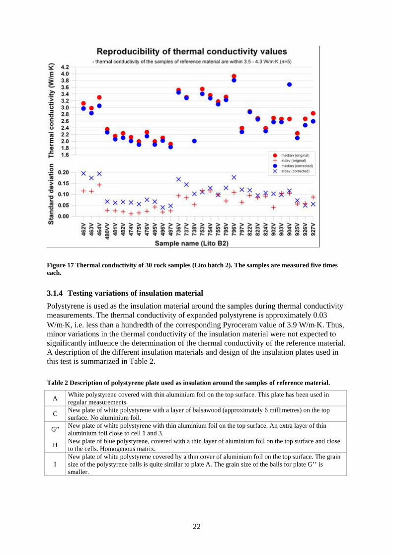
Figure 17 Thermal conductivity of 30 rock samples (Lito batch 2). The samples are measured five times each.

3.1.4 Testing variations of insulation material Polystyrene is used as the insulation material around the samples during thermal conductivity measurements. The thermal conductivity of expanded polystyrene is approximately 0.03 W/m⋅K, i.e. less than a hundredth of the corresponding Pyroceram value of 3.9 W/m⋅K. Thus, minor variations in the thermal conductivity of the insulation material were not expected to significantly influence the determination of the thermal conductivity of the reference material. A description of the different insulation materials and design of the insulation plates used in this test is summarized in Table 2. Table 2 Description of polystyrene plate used as insulation around the samples of reference material.

A White polystyrene covered with thin aluminium foil on the top surface. This plate has been used in regular measurements.

C New plate of white polystyrene with a layer of balsawood (approximately 6 millimetres) on the top surface. No aluminium foil.

G” New plate of white polystyrene with thin aluminium foil on the top surface. An extra layer of thin aluminium foil close to cell 1 and 3.

H New plate of blue polystyrene, covered with a thin layer of aluminium foil on the top surface and close to the cells. Homogenous matrix.

I New plate of white polystyrene covered by a thin cover of aluminium foil on the top surface. The grain size of the polystyrene balls is quite similar to plate A. The grain size of the balls for plate G’’ is smaller.

22

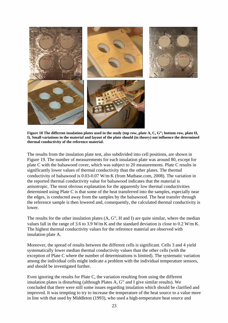
Figure 18 The different insulation plates used in the study (top row, plate A, C, G”; bottom row, plate H, I). Small variations in the material and layout of the plate should (in theory) not influence the determined thermal conductivity of the reference material.

The results from the insulation plate test, also subdivided into cell positions, are shown in Figure 19. The number of measurements for each insulation plate was around 80, except for plate C with the balsawood cover, which was subject to 20 measurements. Plate C results in significantly lower values of thermal conductivity than the other plates. The thermal conductivity of balsawood is 0.03-0.07 W/m⋅K (from Matbase.com, 2008). The variation in the reported thermal conductivity value for balsawood indicates that the material is anisotropic. The most obvious explanation for the apparently low thermal conductivities determined using Plate C is that some of the heat transferred into the samples, especially near the edges, is conducted away from the samples by the balsawood. The heat transfer through the reference sample is then lowered and, consequently, the calculated thermal conductivity is lower. The results for the other insulation plates (A, G”, H and I) are quite similar, where the median values fall in the range of 3.6 to 3.9 W/m⋅K and the standard deviation is close to 0.2 W/m⋅K. The highest thermal conductivity values for the reference material are observed with insulation plate A. Moreover, the spread of results between the different cells is significant. Cells 3 and 4 yield systematically lower median thermal conductivity values than the other cells (with the exception of Plate C where the number of determinations is limited). The systematic variation among the individual cells might indicate a problem with the individual temperature sensors, and should be investigated further. Even ignoring the results for Plate C, the variation resulting from using the different insulation plates is disturbing (although Plates A, G” and I give similar results). We concluded that there were still some issues regarding insulation which should be clarified and improved. It was tempting to try to increase the temperature of the heat source to a value more in line with that used by Middleton (1993), who used a high-temperature heat source and

23

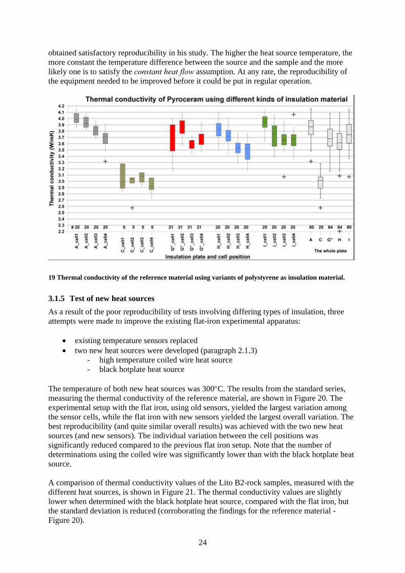
obtained satisfactory reproducibility in his study. The higher the heat source temperature, the more constant the temperature difference between the source and the sample and the more likely one is to satisfy the constant heat flow assumption. At any rate, the reproducibility of the equipment needed to be improved before it could be put in regular operation.

Figure

19 Thermal conductivity of the reference material using variants of polystyrene as insulation material.

3.1.5 Test of new heat sources ility of tests involving differing types of insulation, three

paragraph 2.1.3)

h °C. The results from the standard series,

e heat

rison of thermal conductivity values of the Lito B2-rock samples, measured with the

As a result of the poor reproducibattempts were made to improve the existing flat-iron experimental apparatus:

• existing temperature sensors replaced • two new heat sources were developed (

- high temperature coiled wire heat source - black hotplate heat source

T e temperature of both new heat sources was 300measuring the thermal conductivity of the reference material, are shown in Figure 20. The experimental setup with the flat iron, using old sensors, yielded the largest variation among the sensor cells, while the flat iron with new sensors yielded the largest overall variation. Thebest reproducibility (and quite similar overall results) was achieved with the two new heat sources (and new sensors). The individual variation between the cell positions was significantly reduced compared to the previous flat iron setup. Note that the number of determinations using the coiled wire was significantly lower than with the black hotplatsource.

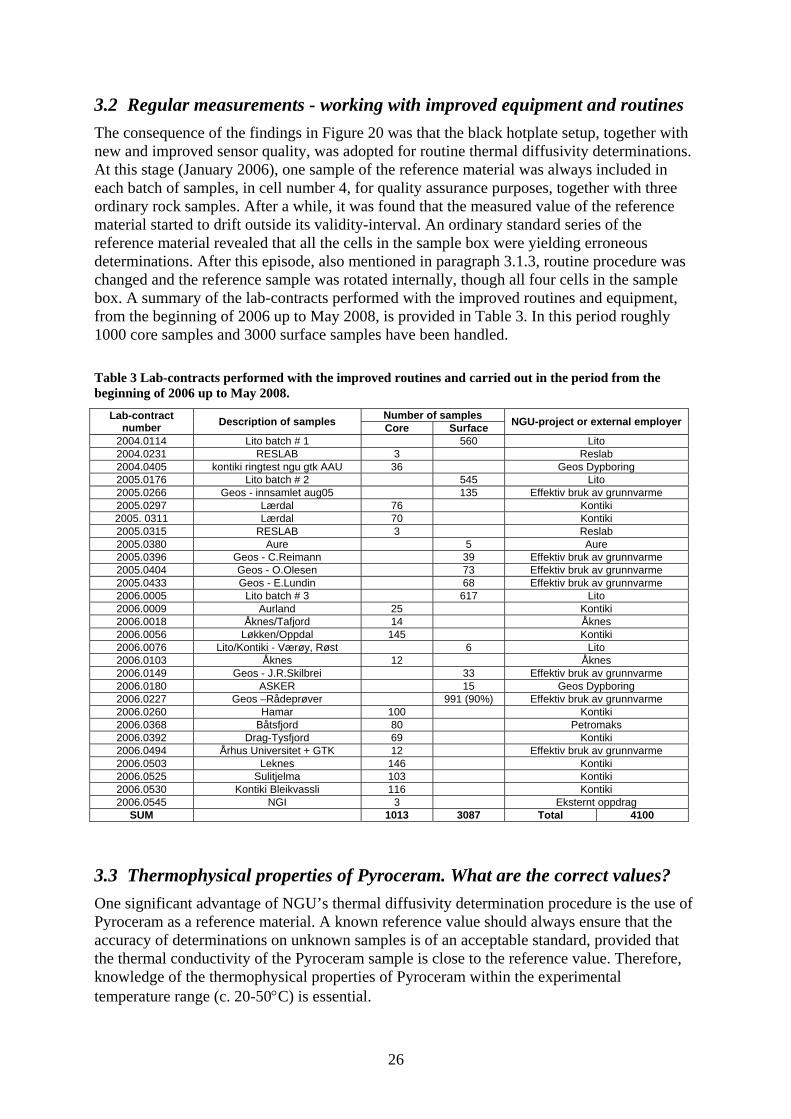
compaAdifferent heat sources, is shown in Figure 21. The thermal conductivity values are slightly lower when determined with the black hotplate heat source, compared with the flat iron, but the standard deviation is reduced (corroborating the findings for the reference material - Figure 20).

24

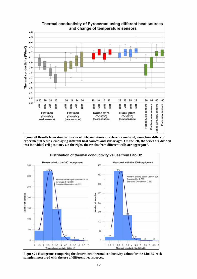
Figure 20 Results from standard series of determinations on reference material, using four different xperimental setups, employing different heat sources and sensor ages. On the left, the series are to individual cell positions. On the right, the results from different cells are aggregated.

e divided

Figure 21 Histograms comparing the determined thermal conductivity values for the Lito B2-rock samples, measured with the use of different heat sources.

in

25

3.2 Regular measurements - working with improved equipment and routines The consequence of the findings in Figure 20 was that the black hotplate setup, together with new and improved sensor quality, was adopted for routine thermal diffusivity determinations. At this stage (January 2006), one sample of the reference material was always included in each batch of samples, in cell number 4, for quality assurance purposes, together with three ordinary rock samples. After a while, it was found that the measured value of the reference material started to drift outside its validity-interval. An ordinary standard series of the reference material revealed that all the cells in the sample box were yielding erroneous determinations. After this episode, also mentioned in paragraph 3.1.3, routine procedure was changed and the reference sample was rotated internally, though all four cells in the sample box. A summary of the lab-contracts performed with the improved routines and equipment, from the beginning of 2006 up to May 2008, is provided in Table 3. In this period roughly 1000 core samples and 3000 surface samples have been handled. Table 3 Lab-contracts performed with the improved routines and carried out in the period from the beginning of 2006 up to May 2008.

Lab-contract number Description of samples Number of samples NGU-project or external employer Core Surface

2004.0114 Lito batch # 1 560 Lito 2004.0231 RESLAB 3 Reslab 2004.0405 kontiki ringtest ngu gtk AAU 36 Geos Dypboring 2005.0176 Lito batch # 2 545 Lito 2005.0266 Geos - innsamlet aug05 135 Effektiv bruk av grunnvarme 2005.0297 Lærdal 76 Kontiki 2005. 0311 Lærdal 70 Kontiki 2005.0315 RESLAB 3 Reslab 2005.0380 Aure 5 Aure 2005.0396 Geos - C.Reimann 39 Effektiv bruk av grunnvarme 2005.0404 Geos - O.Olesen 73 Effektiv bruk av grunnvarme 2005.0433 Geos - E.Lundin 68 Effektiv bruk av grunnvarme 2006.0005 Lito batch # 3 617 Lito 2006.0009 Aurland 25 Kontiki 2006.0018 Åknes/Tafjord 14 Åknes 2006.0056 Løkken/Oppdal 145 Kontiki 2006.0076 Lito/Kontiki - Værøy, Røst 6 Lito 2006.0103 Åknes 12 Åknes 2006.0149 Geos - J.R.Skilbrei 33 Effektiv bruk av grunnvarme 2006.0180 ASKER 15 Geos Dypboring 2006.0227 Geos –Rådeprøver 991 (90%) Effektiv bruk av grunnvarme 2006.0260 Hamar 100 Kontiki 2006.0368 Båtsfjord 80 Petromaks 2006.0392 Drag-Tysfjord 69 Kontiki 2006.0494 Århus Universitet + GTK 12 Effektiv bruk av grunnvarme 2006.0503 Leknes 146 Kontiki 2006.0525 Sulitjelma 103 Kontiki 2006.0530 Kontiki Bleikvassli 116 Kontiki 2006.0545 NGI 3 Eksternt oppdrag

SUM 1013 3087 Total 4100

3.3 ophy f Pyr am. arOne significant advantage of NGU’s thermal d usivity de rmination procedure is the use of Pyr s a re own raccuracy of determ n samples is of an ptable t the onductivity o yroceram sam is close to the reference value. Therefore, knowledge of the thermophysical properties of Pyroceram ithin the experi tem range (c. sential.

Therm sical properties o ocer What e the correct values? iff te

oceram a ferenc . A kne material eference value should always ensure that the inations on unknow acce standard, provided tha

thermal c f the P ple w mental

perature 20-5 is es0°C)

26

However, finding an unequivocal set of thermo hysical properties for Pyroceram has been a daunting task. Since:

ermal lated a e produ of specific heat capacity (Cp), ty (ρ) an ivity (α) ( quation 1 nd GU equi ines therm

the our search urned towar reliable alue for the th usivity of Pyr ather t uctivit he only rameterexh imal variation with temperature is density, ρ=2600 kg/m . Specific heat capacity and diffusivit nificantly hin the experimental temperature range. An inte everal interesting studies, especially oneertif n of Pyroceram a a reference material. Contacts with som he involversons, in the beginning of 2006, revealed the complexity of this large study, but some of

their reported values for thermal diffusivity were in agreement with NGU’s results from

d l

, respectively (Salmon et al, 2007). Note

[m2/s]

n 9

l.

p

1. the th conduc is calcutivity s th c tdensi d thermal diffus E ), a

2. the N pment actually determ al diffusivity,

focus of g tradually ds a v ermal diffoceram, r han its thermal cond y. T pa in Equation 1 that

3ibits min thermal y both vary sig witrnet-based search revealed s concerning

cp

icatio s e of t ed

standard series measurements (paragraph 3.1.5). Thus, while waiting for certification of Pyroceram as a reference material to be agreed, the preliminary reported values were used as a guideline. Finally in March 2007, certified values for thermal conductivity (λ) and thermal diffusivity (α) up to 1025 K were released for Pyroceram/BCR-724 from the European Commission, Directorate-General Joint Research Centre, Institute for Reference Materials anMeasurements in Belgium. Here, the certified values for thermal conductivity (λ) and thermadiffusivity (α), as a function of temperature and valid for temperatures between 298 K and 025 K, are expressed in Equation 9 and Equation 101

that, in Salmon et al. (2007), the denotation of thermal conductivity is λ instead of K.

41238252 10147.410541.110133.210351.1406.4 TTTT ⋅⋅+⋅⋅−⋅⋅+⋅⋅−= −−−−α

Equatio

Uncertainty is 6.1 % with coverage factor k=2 at 95% confidence leve

T1.515332.2 +=λ [W/m⋅K]

Equation 10

Uncertainty is 6.5 % with coverage factor k=2 at 95% confidence level. In both equations, T is absolute temperature in Kelvin. Specific heat capacity was also measured by six laboratory partners, and within the temperature range 298-1273K, the average values over all laboratories can be represented

by

at apacity and thermal diffusivity) in the temperature range of 20-50°C. A box-plot of

results from the standard series, measured with the reconfigured equipment with newtemperature sensors and the black hotplate heat source at 300°C (Figure 20), is show

Equation 11 (Salmon et al., 2007).

41339263 101295.610497.210878.310923.22334.0 TTTTCp ⋅⋅−⋅⋅+⋅⋅−⋅⋅+= −−−− [J/(g⋅K)]

Equation 11

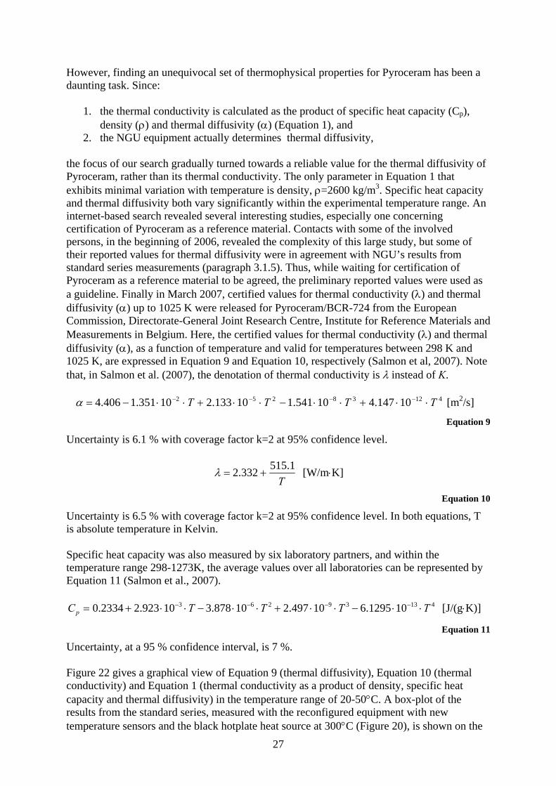
Uncertainty, at a 95 % confidence interval, is 7 %. Figure 22 gives a graphical view of Equation 9 (thermal diffusivity), Equation 10 (thermal onductivity) and Equation 1 (thermal conductivity as a product of density, specific hec

c the n on the

27

right axis. Some selected values of specific heat capacity (from Equation 11) are listed to the ght.

The temperature range considered in Figure 22 is thought to represent real conditions in the sample during experimental determination. The temperature signal is always measured at the base of the sample (Figure 9), and the 300°C heat source is placed approximately 1

around 20°C and the maximum stop temperature is 40°C. is difficult to estimate the real temperature at the top of the sample surface during the

sensor,

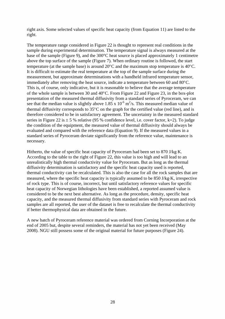
ut it is reasonable to believe that the average temperature f the whole sample is between 30 and 40°C. From Figure 22 and Figure 23, in the box-plot

presentation of the measured thermal diffusivity from a standard series of Pyrocerasee that the median value is slightly above 1.85 x 10-6 m2/s. This measured median value of thermal diffusivity corresponds to 35°C on the graph for the certified value (red lin

. The uncertainty in the measured standard eries in Figure 22 is ± 5 % relative (95 % confidence level, i.e. cover factor, k=2). To judge

is

ing to the table to the right of Figure 22, this value is too high and will lead to an nrealistically high thermal conductivity value for Pyroceram. But as long as the thermal

t

ty

ri

centimetre above the top surface of the sample (Figure 7). When ordinary routine is followed, the start temperature (at the sample base) is Itmeasurement, but approximate determinations with a handheld infrared temperatureimmediately after removing the heat source, indicate a temperature between 60 and 80°C. This is, of course, only indicative, bo

m, we can

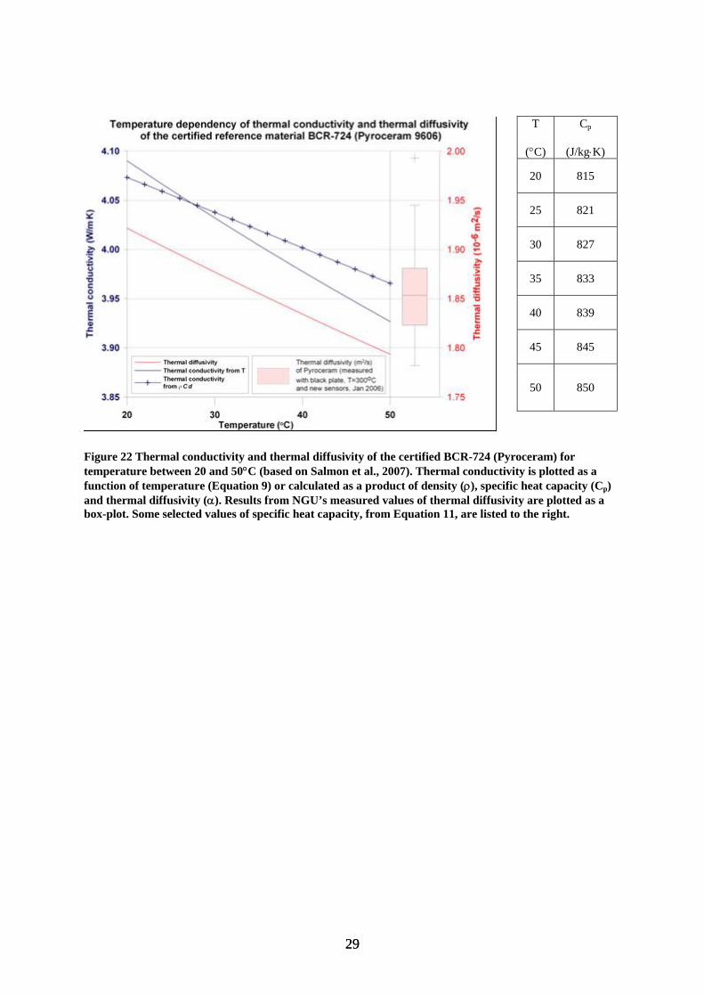
e), and is therefore considered to be in satisfactory agreementsthe condition of the equipment, the measured value of thermal diffusivity should always be evaluated and compared with the reference data (Equation 9). If the measured values in a standard series of Pyroceram deviate significantly from the reference value, maintenance necessary. Hitherto, the value of specific heat capacity of Pyroceram had been set to 870 J/kg⋅K. Accordudiffusivity determination is satisfactory and the specific heat capacity used is reported, thermal conductivity can be recalculated. This is also the case for all the rock samples that aremeasured, where the specific heat capacity is typically assumed to be 850 J/kg⋅K, irrespective of rock type. This is of course, incorrect, but until satisfactory reference values for specific heat capacity of Norwegian lithologies have been established, a reported assumed value is considered to be the next best alternative. As long as the procedure, density, specific heacapacity, and the measured thermal diffusivity from standard series with Pyroceram and rocksamples are all reported, the user of the dataset is free to recalculate the thermal conductiviif better thermophysical data are obtained in the future. A new batch of Pyroceram reference material was ordered from Corning Incorporation at the end of 2005 but, despite several reminders, the material has not yet been received (May 2008). NGU still possess some of the original material for future purposes (Figure 24).

28

T

(°C)

Cp

(J/kg⋅K)

20 815

29

25 821

30 827

35 833

40 839

45 845

50 850

Figure 22 Thermal conductivity and thermal diffusivity of the certified BCR-724 (Pyroceram) for temperature between 20 and 50°C (based on Salmon et al., 2007). Thermal conductivity is plotted as a function of temperature (Equation 9) or calculated as a product of density (ρ), specific heat capacity (Cp) and thermal diffusivity (α). Results from NGU’s measured values of thermal diffusivity are plotted as a box-plot. Some selected values of specific heat capacity, from Equation 11, are listed to the right.

29

as

Figure 24 Remnant Pyroceram material held by NGU.

3.4 Ring test of thermal conductivity As a part of NGU’s quality assurance procedure, a ring test has been performed, involving the University of Aarhus in Denmark, the Geological Survey of Finland (GTK) and NGU. The laboratories in Denmark and Finland use the needle probe method (Balling et al., 1981) and the divided bar method (Kukkonen and Lindberg, 1995), respectively. Both methods are considered more accurate than the transient method used by NGU. The major advantage of the NGU-equipment is the rapid measurement of several samples in one batch. Three rock samples and one reference material are measured in 200 seconds, which greatly enhances the capacity of the laboratory.

Figure 23 Results from standard series of Pyroceram/BCR-724: similar to Figure 20 but here presented thermal diffusivity rather than thermal conductivity.

30

From the results in Figure 26, the determinations from the three laboratories can be seen, with a few exceptions, to be in good agreement. The rock samples used in the ring test were divided into an A- and B-sample, and then sub-divided again into two parts for a pair of laboratories. The University of Aarhus and NGU carried out determinations on most samples, while GTK is represented by about the half of the rock samples. The samples from Flå, Hjerkinn and Hurdal 2-4 appear to yield the most consistent determinations, while the largest deviations can be seen for Lærdal 1A, Mistberget 2A, Lærdal 2A and Hurdal 2A. A large variation is also observed for the Høgtuva samples, although this is likely to be related to foliation. The Høgtuva samples exhibiting the lowest values are measured with a heat flux normal to the foliation, while those with the highest thermal conductivity are measured parallel to the foliation. The average value for the Høgtuva samples is, of course, intermediate. The thermal conductivity of Lærdal 1, as measured in Aarhus, is 2.1 W/m·K while the corresponding value from NGU for both Lærdal 1A and 1B is 2.7 W/m·K - a difference of 0.6 W/m·K or 25 % of the average value. The discrepancy can be explained in several ways:

1. The Lærdal samples are characterised as gneisses, which, due to inhomogeneity and foliation, can exhibit significant mineralogical and structural variation.

2. The deviation may simply represent either random or systematic error, occurring in the lower range of thermal conductivity values.

Almost the same relation is found for Mistberget 2A, where the Aarhus value is 2.2 W/m·K and the NGU value is 2.6 W/m·K - a discrepancy of 0.4 W/m·K or 17 % of the average value.

/m·K - even lower than the Aarhus-value. From the sample photographs in Figure 25, we an see that the mineral composition of Mistberget 2A differs significantly from the syenites

Mistberget 3A and 4A. Mistberget 2A is probably a siltstone. Lærdal 2A exhibits more or less the same behaviour as Lærdal 1A. The University of Aarhus returned the lowest value of 2.7 W/m·K, while NGU’s determination for both the A and B samples was 3.1 W/m·K - a discrepancy of 0.4 W/m·K or 14 % of the average value. The first measurement of Hurdal 2A carried out by NGU was much lower than the result from the University of Aarhus. The sample was thus re-measured at NGU. The second measurement turned out to be consistent with the Aarhus result (Figure 26), and the first

ror and should be neglected in the further

t pairs of samples. The results from GTK were

As an extra quality control, the Mistberget 2A-sample was re-measured at NGU with exactly the same result as before at NGU. The value of Mistberget 2B, measured by GTK, is 2.0 Wc

measurement was therefore considered to be in eranalysis. All three laboratories were represented by eighsystematically lower than those from the University of Aarhus and NGU, except for one pair of samples. For Hurdal 2 all three laboratories (provided that the first, erroneous measurement from NGU is neglected) achieved very consistent results. In six of the eight cases (Hurdal 1, Løkken 2 and Mistberget 1-4), the GTK-value is around 0.1-0.3 W/m·K lower than the corresponding Aarhus- or NGU-values. This could imply that the GTK-results are systematically lower, that the Aarhus- and NGU-values are systematically higher, or maybeboth.

31

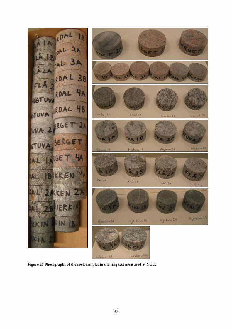
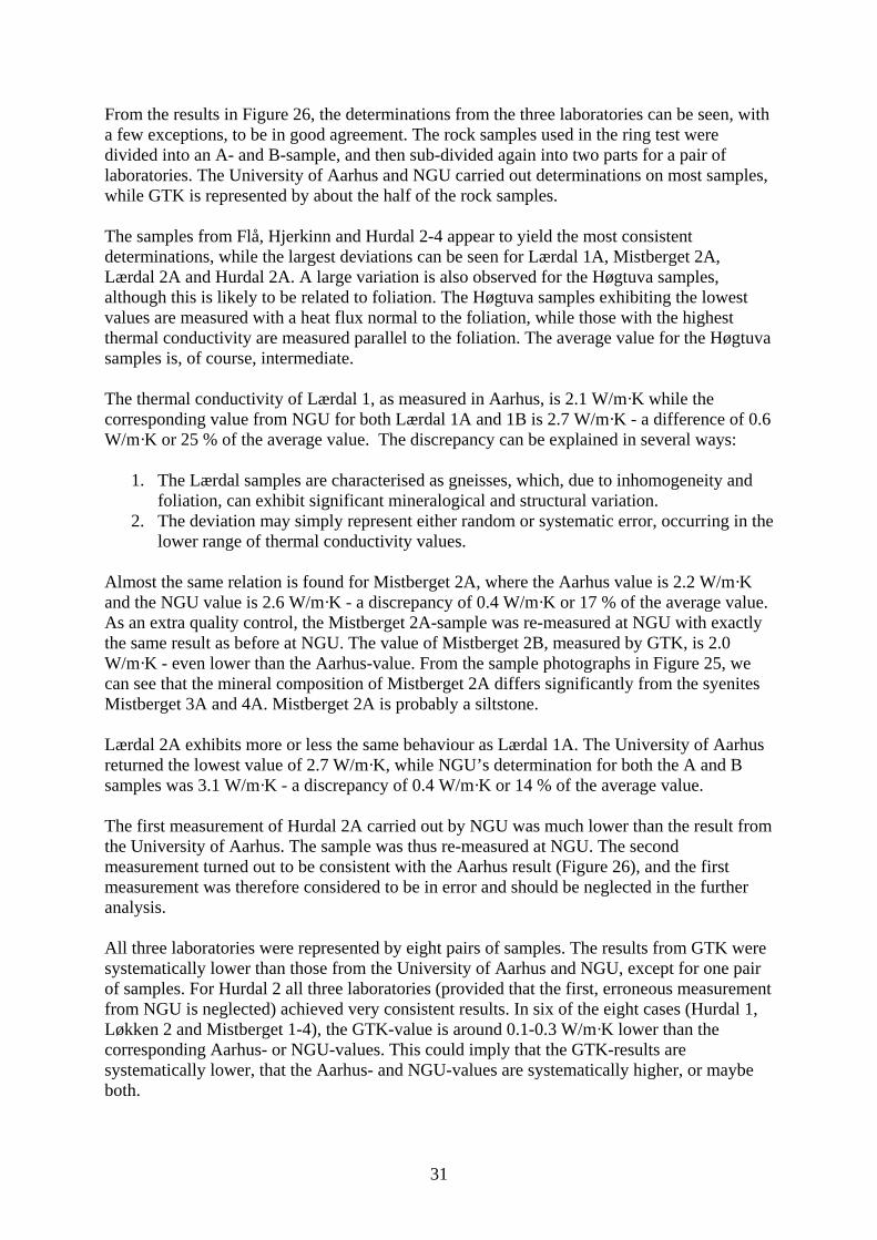
Figure 25 Photographs of the rock samples in the ring test measured at NGU.

32

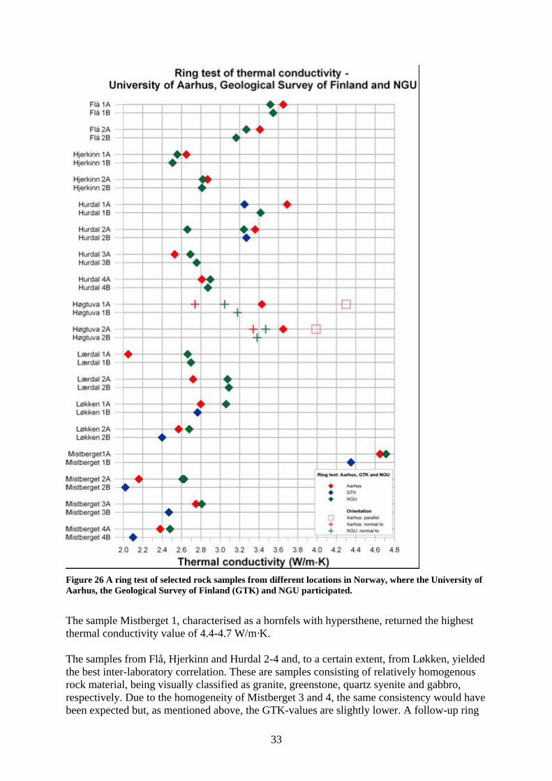
Figure 26 A ring test of selected rock samples from different locations in Norway, where the University of Aarhus, the Geological Survey of Finland (GTK) and NGU participated.

The samples from Flå, Hjerkinn and Hurdal 2-4 and, to a certain extent, from Løkken, yielded the best inter-laboratory correlation. These are samples consisting of relatively homogenous rock material, being visually classified as granite, greenstone, quartz syenite and gabbro, respectively. Due to the homogeneity of Mistberget 3 and 4, the same consistency would have been expected but, as mentioned above, the GTK-values are slightly lower. A follow-up ring

The sample Mistberget 1, characterised as a hornfels with hypersthene, returned the highest al conductivity value of 4.4-4.7 W/m·K. therm

33

test, where the thermal properties of Pyroceram will be determined, is in progress, but the results are not yet available. It should be noted that the values of specific heat capacity for the different rock samples utilised by the laboratories in Aarhus and GTK are not known. In fact, the divided bar method used at GTK determines thermal conductivity directly. NGU and the University of Aarhus measure the thermal diffusivity and thereafter calculate the thermal conductivity from Equation 1. NGU assumes a generic value for specific heat capacity of 850 J/kg⋅K for all rock types. Thus, a better comparison of the results from the three laboratories would have been achieved if the specific heat capacity values were known. This would have allowed a comparison of thermal diffusivity as well as thermal conductivity.

3.5 Linear segment of the temperature-time curve? Accumulated experienced from regular operation has suggested that the calculated values of thermal diffusivity might be sensitive to the location and “width” of the time window selected for determining the maximum slope of the temperature evolution curve between two defined points. Thus, the linearity of the temperature-time curve (which yields thermal diffusivity from Equation 4, as described in paragraph 2.2) has been examined at several stages. Figure 27 illustrates a measurement performed in 2005, using the 2001 version of the equipment. The measured (bright red line) and modelled (blue crosses) temperature-time curves seem to fit well to a linear function (orange line). However, from the slope it can be seen that neither the measured (blue dots) nor the modelled (dark red line) slope (m), are completely constant after the initial temperature-rise period. To be entirely linear, the value of the slope m should be constant for a defined interval of time. As it can be seen from the blue dots of the measured slope m, the temperature evolution appears to be stepwise, and thus reflects the accuracy of the temperature sensors. Improved resolution of the temperature sensors and a shorter sampling interval would perhaps improve the accuracy of the temperature-time curve analysis and thereby the accuracy of the calculated thermal diffusivity.

Figure 27 Analysis of temperature-time data from a specific test (using the flat iron equipment) implies that the linearity of the temperature-time curve is not perfect and that temperature data collection routines could be improved.

34

The questions raised in this context were explored by numerical modelling of the entire

ethod and equipment (paragraph 3.6).

scale te element modelling

software FEFLOW 5.2. The objectives of the study were to achieve a better understanding of sign, accuracy and procedures. r the experimental

,

ear

e samples in the multiple ample configuration, showed that the error is around 0.5 to 1.5 %. In this simulation, the rock

samples were modelled using varying thermal conductivity values, ranging from 0.5 to 2.0 times the standard value of Pyroceram. It should be noted that FEFLOW® is not able to simulate heat transfer by radiation, only by conduction. Therefore, the assumption of a constant heat flux onto a semi-infinite slab (Carslaw and Jaeger, 1959) used by Middleton (1993) is translated directly as a constant boundary condition in the modelling exercise. The model simulations lead us to believe that, during a measurement, temperature evolution within the insulation and its influence on the rock samples may be so large that the validity of the analytical approximation becomes doubtful. An apparatus whose heat source provides a constant heat flux onto the sample surfaces only (and not onto the insulation), would be a preferred option for the future. Although the reproducibility of the current method and equipment is considered to be acceptable, the modelling provided valuable understanding of the ongoing thermal processes and suggested that some specific improvements should be considered: • Reducing the sample thickness to a maximum of 1 cm. • Minimizing the time interval between the temperature measurements

m

3.6 Modelling of the apparatus and the dynamics during a measurement The Section is mainly based on work by De Beer (2006). To explore the questions raised by the above quality assurance work, a numerical full 3D-model of the laboratory equipment was generated using the fini

®

the ongoing thermal processes and to improve experimental deAmong others issues, the validation of the 1D-approximation foconfiguration, the constant heat flux approximation and the choice of materials for the devicewere addressed. A few model simulations considered the sensitivity of the best fit method to identify the linsegment of the temperature-time curve as described in paragraph 2.2 and 3.5. The results showed that increasing the time intervals between the temperature measurements reduces the accuracy with which the linear segment is established and leads to an overestimation of thermal diffusivity and thermal conductivity. To overcome this problem, a sufficiently long measurement period is required to obtain a significant length of the linear segment. 3D-simulation of varying sample thicknesses, showed that an increased sample thickness, from 1 to 2 centimetres, leads to an overestimation of the actual thermal diffusivity, and thusof the thermal conductivity, by almost 7%. A model simulation of possible thermal interference between ths

• Using an alternative insulation material to polystyrene to avoid melting. • Increasing the distance between the individual samples.

35

Hitherto, none of these suggested improvements have been implemented, but the most a

definition of the linear segment of the temperature-me curve used for analysis. A few tests with reduced sample thickness have been performed,

but have proved to yield rather inaccurate results. A sample thickness of 1 cm reduces the of

reducing the sample thickness is e inhomogeneity and representativity of the sample material. The equipment has the

cations;

realistic initiative would be to increase the number of temperature measurements during determination. This will lead to improvedti

measurement time significantly, and thus results in inaccuracy due to the limited numbertemperature measurements on the temperature-time curve (in turn, causing difficulties inidentification of the linear segment). Another drawback ofthobjective of determining the thermal properties of whole rocks, and a thinner sample will overestimate the influence of irregularities such as large mineral grains, veins etc. An alternative insulation material and increased distance between the individual samples will be considered for future implementation, together with more comprehensive modifie.g. the design of a new sample box to make the measurement process more effective.

36

4. Discussion

A series of tests and analyses have been performed using NGU’s equipment for measuring thermal diffusivity to:

1. increase our understanding of the thermal processes involved, and 2. improve experimental routines and reproducibility.

There remain some specific improvements that can be implemented. This chapter will discuss and evaluate the various tests performed. The thermal properties of rock samples from Norwegian bedrock are not easily determined. At laboratory scale, the sample material is often inhomogeneous and anisotropic: the rock samples may be layered, foliated, lineated or structured in other ways, leading to anisotropy on scales of a few cm. With this in mind, and with the goal of obtaining a reasonable understanding of the distribution of thermal conductivity, either with depth in a cored borehole or at the bedrock surface, the number of samples analysed is a critical factor. Thus, many samples determined with “adequate” analytical quality might be preferable to a few samples determined at high accuracy. Part of the quality assurance procedure implemented by NGU for thermal diffusivity determination is the use of a certified reference material whose thermal diffusivity is within the expected range of values for real rocks. The certification of Pyroceram at IRRM last year (Salmon et al., 2007), here called BCR-724, represented a breakthrough and ensures a robust quality control on all samples measured. The sum of single initiatives performed over the past few years has resulted in overall improved reproducibility of measured values (although it would be difficult to identify some improvements as more effective than others). Probably the three most important improvements have been:

• increased temperature of the heat source, • more robust temperature sensors • the use of acceptance criterion instead of a correction factor.

The initial tests, described in paragraph 3.1, were mainly founded on the concern that the test procedure was producing erroneous results and poor reproducibility (Figure 13). They can be characterised as a search for sources of error and the start of NGU’s understanding of the heat transfer mechanisms within the experimental apparatus. It seemed to be the case that, rather than being influenced by type of insulation, resting time of the reference material, diurnal climatic variations or other ambient factors, the apparent experimental errors could be better described as “random”. The modification of procedure, involving the use of an acceptance criterion rather than a correction factor, was a more straightforward decision based on two considerations:

37

1. Firstly, a reproducibility analysis of 30 rock samples from the Lito B2-contract ncorrected values had lower standard deviations than the corresponding es (paragraph 3.1.3 and Figure 17).

2. Secondly, the use of acceptance criteria is widely practised throughout NGU-lab, and seems to be the most appropriate way to ensure reproducibility, while minimising time

at all the measurements have been subject to a quality assurance ce criterion must ere the four

dif ed in the sample box. An

ew temperature sensors are installed. During n

ually,

d er than the 144°C of the flat iron originally used by

o indicate that reproducibility is improved by the s of

the certified values within the experimental temperature range om theory, the black hotplate (300°C) flat iron (144°C) and seems to have

with the flat iron, the irds, from 600 to 200

rison would have been achieved if the values of rock specific heat

ity easured conductivity increases with increasing sample thickness), as determined by the

showed that ucorrected valu

consumption and other possible error sources.

his method requires thTprocedure relying on a known value of the reference material. The acceptan

asurements, whbe defined in advance by performing a standard series of mef rent samples of reference material (kal_20-23) are rotate

adequate number of measurements enables a statistical determination of the standard deviation, from which the acceptance criterion or alarm level is calculated (Equation 7). The cceptance criterion is recalculated when na

routine measurements of rock samples, the reference sample is rotated in different cells withithe sample box and is used to identify deviating results related to a specific temperature sensor. Batches of measurements where the thermal conductivity of the reference sample is outside the acceptance criterion are rejected. Several rejected measurements within a limited period indicate that something is wrong and that corrective action must be initiated. Usthe sensors are worn out and must be replaced. The temperature of the coiled-wire heat source used in the experimental apparatus describe

iddleton (1993) must have been highMNGU. Placing the heat source about 1 cm above the sample surface is considered to beequivalent to an oven effect (Carslaw and Jaeger, 1959, in Middleton, 1993) and a constant heat flux boundary condition is approximately realized (Middleton, 1993). By replacing NGU’s flat iron with a black hotplate of temperature of 300°C, the apparatus is almost identical to the setup of Middleton (1993) and the constant heat flux assumption is better pproximated. The results in Figure 20 alsa

use of a higher temperature source. According to the certified thermal diffusivity valuePyroceram/BCR-724 (Figure 22), the introduction of the black hotplate heat source seems to be beneficial in terms of accuracy as well. The values measured using the black hotplate correspond satisfactorily with the certified values, while the values obtained using the flat iron

eat source are lower than h(Figure 23 and Figure 22). Thus, just as expected fr

than thebetter approximates to a constant heat fluximproved both experimental reproducibility and accuracy. Compared se of the black hotplate also reduces the measurement time by two-thu

seconds. The ring test between NGU and the thermal conductivity labs of the University of Aarhus and Geological Survey of Finland (GTK) confirmed that the NGU determinations are of satisfactory quality. All three laboratories yielded some deviating results that, to a large extent, can be related to the inhomogeneous or anisotropic structure and composition of the rock samples. The results are particularly sensitive to foliation. It should also be noted that a

ore meaningful compamcapacity assumed by the Aarhus and GTK labs had been known.

idttømme et al. (2000) reported that sample thickness influenced thermal conductivM(m

38

1998-version of NGU’s equipment. Modelling in FEFLOW® confirms this trend and it iprobably ultimately related to the semi-infinite slab assumption (Chapter

s

uld be upgraded. The modelling of the quipment setup and the dynamics of the thermal processes in FEFLOW® led to a better

e,

the ntly,

ear

hickness of the sample. This should more nearly approximate the semi-infinite slab assumption of thermal conductivity theory

e s will

o e

he

ht

as been performed concerning the quality of NGU’s routines and equipment for

in ber of samples is

od is

1). NGU’s equipment for the determination of thermal diffusivity and the calculation of thermal conductivity may still be open to improvement. In particular, the procedure for calculating thermal diffusivity from the temperature-time curve shoeunderstanding and suggested some further improvements. Evaluating the study as a wholincluding the modelling, the potential improvements should be prioritized as follows: • Increase the number of temperature readings per determination. This is regarded as

single most effective initiative to increase the reproducibility of the method. Curretemperature logging is performed every 2.8 seconds, but we recommend an interval of every 0.5 or 1 seconds. More temperature data will allow a better definition of the linsegment of the temperature-time curve with the steepest slope. This will, in turn, improve the accuracy of the thermal diffusivity calculation (Equation 4).

• Increase the distance between individual samples. This should reduce any interference between samples in the box. Quantification of the new centre distances should be determined from modelling.

• Increase the sample diameter or reduce the t

(Carslaw and Jaeger, 1959, in Middleton, 1993), and will possibly improve experimental reproducibility further. A reduction in the sample thickness could, however, induce morinaccuracies, as mentioned in paragraph 3.6. Any inhomogeneity in the rock samplebe more significant in smaller samples. A reduced sample thickness will also reduce the measurement time, and thus the number of available temperature readings (required tensure a proper definition of the linear segment of the temperature-time curve for thestimation of thermal diffusivity).

• The degree of reflection of heat from rock sample surfaces of varying colour / albedo is unknown, and should be tested, for example, by applying graphite powder to the top of tsamples. If the difference in heat absorption between dark and bright rock samples varies significantly, this will lead to erroneous estimates of thermal conductivity for the brigrock types. Reflection caused by irregular surfaces should also be considered.

5. Conclusions

study hAdetermining thermal diffusivity. Thermal conductivity is estimated from diffusivity using Equation 1. The conclusions from the study can be summarized as follows: • NGU’s laboratory equipment for determining thermal diffusivity of rock samples is

considered to deliver satisfactorily reproducible results. Some rock types of inhomogeneous and anisotropic nature can yield varying results depending on sample orientation and mineral composition. For mapping purposes, either in three dimensions a cored borehole or in two dimensions as surface mapping, a large numregarded as more important than a few results with high reproducibility. NGU’s methrapid and satisfies an increasing demand for thermal conductivity data.

39

• A significant advance with respect to reproducibility and accuracy for the NGU methodology is the adoption of a certified reference material BCR-724 (Pyroceram). BCR-724 has been certified by the Joint Research Centre, Institute for Reference

ng

.

ed accuracy. New temperature sensors and a new heat source have been installed. The

ck ad

conforms to

e also the measurement time is reduced from 600 to 200 seconds.

the

in

the whole study, the most important priority to

Materials and Measurements for the European Commission (Salmon et al., 2007). As longas the quality assurance procedures are followed, based on acceptance criteria, and as loas the results are in harmony with the certified values, the quality of determination of thermal diffusivity of rock samples by the NGU equipment is regarded as satisfactory

• Two modifications to the equipment are considered to have been important for improvedreproducibility and (according to certified values of the reference material) improv

temperature sensors are considered to be more robust and flexible and to ensure a good contact between the bottom of the rock sample and the temperature sensor. The new blahotplate heat source has a temperature of 300°C. The previous heat source, a flat iron, ha temperature of only 144°C. Figure 23 confirms that the new heat source improved the reproducibility, and compared with Figure 22, also the accuracy of the method. It is believed that the temperature of the new heat source more closelyMiddleton's (1993) setup, and that the constant heat flux boundary condition is more closely approximated (Middleton, 1993). The higher temperature of the heat sourcmakes the method faster, and From Figure 23 it can also be seen that the new temperature sensors appear to improveaccuracy slightly.

• A ring test between the University of Aarhus, the Geological Survey of Finland and NGU confirmed that the NGU-results are within the range of the other laboratories and have satisfactory quality. A follow-up, where the thermal properties of Pyroceram/BCR-724 areexamined, is in progress, but not yet completed.

• Modelling in FEFLOW® led to a better understanding of the ongoing thermal processesthe apparatus and has indicated some potential for improved design, accuracy and experimental procedure. Evaluatingimprove the quality of the determinations is to increase the temperature logging frequency. This will ensure a more robust definition of the linear segment of the temperature-time curve which is used for the calculation of the thermal diffusivity.

40

41

ity

-

pages.

of rocks.

8. Mills, A.F (1995): Heat and mass transfer. The Richard D. Irwin series in heat transfer,

Chicago, Irwin, 1240 pages. 9. Midttømme, K., Ramstad, R.K. Solli, A. Sørdal, T. and Elvebakk, H. (2004):

Grunnvarmekartlegging i Asker og Bærum. NGU-report 2004.013, 44 pages. 10. Midttømme, K. Hilmo, B.O, Skarphagen, H. and Nissen, A. (2000): Kartlegging av

energipotensialet i berggrunnen på kartblad Bekkestua, Bærum kommune: Varmeledningsevnen til bergarter. NGU-report 2000.036, 105 pages.

11. Salmon, D., Roebben, G., Lamberty, A. and Brandt, R. (2007): Certification of thermal

conductivity and thermal diffusivity up to 1025 K of a glass-ceramic reference material BCR-724. Report EUR 21764 EN. European Commission, Directoreate-General, Joint Research Centre, Institute for Reference Materials and Measurements, 73 pages.

12. Wissing, B.W. and Ramstad, R.K. (2006): Labprosedyrer knyttet til måling av

varmeledningsevne per desember 2006. Internt dokument ved NGU, 24 pages.

6. References

Balling, N., Kristiansen, J.I., Breiner, N., Poulsen, K.D., Rasmussen, R. & Saxov, S. 1.1981: Geothermal measurements and subsurface temperature modelling in Denmark. GeoSkrifter 16, 172 pp. Århus, Denmark: University of Aarhus.

2. Beer, H. de., (2006): A transient method for measuring thermal properties of rocks – a heat flow model to support laboratory experiments. Presentation at the Advanced FEM Groundwater Modelling, International FEFLOW User Conference, Berlin, 5 pages.

3. Carslaw, H.S, and Jaeger, J.C., (1959): Conduction of heat in solids. Oxford UniversPress, Inc, 510 pages.

4. Grimstvedt, A, Ødegård, M. and Davidsen, B. (2005): NGU-Lab fellesdokumenter. NGU

SD 1-3: Produksjonsrutiner. Seksjon 1.3.12: Veiledning og rutiner ved statistisk behandling av data. Norges geologiske undersøkelse, Faggruppe for laboratorier, 77 pages.

5. Kukkonen I. and Lindberg A. 1995. Thermal conductivity of rocks at the TVO

investigation sites Olkiluoto, Romuvaara and Kivetty. Nuclear Waste Commission of Finnish Power Companies, Report YJT-98-08, 29

6. Matbase (2008): Material data for balsa. Online:

http://www.matbase.com/material/wood/class4-5-10-years/balsa/properties.

7. Middleton, M.F. (1993): A transient method of measuring the thermal properties Geophysics, Vol. 58, No. 3, p. 357-365.

Date post:	23-Feb-2022
Category:	Documents
Upload:	others
View:	12 times
Download:	0 times

NGU Report 2008.050 Thermal diffusivity measurement at NGU

Documents