55
NIFS Data Reduction Richard McDermid South American Gemini Data Workshop São José dos Campos, Brazil, October 27-30, 2011
| Date post: | 18-Dec-2015 |
| Category: |
Documents |
| View: | 217 times |
| Download: | 2 times |

NIFS Data Reduction
Richard McDermidSouth American Gemini Data Workshop
São José dos Campos, Brazil, October 27-30, 2011

IFU Zoo: IFU Zoo: How to map 3D on How to map 3D on 2D2D
“Spaxel”
NIFSNIFS
2
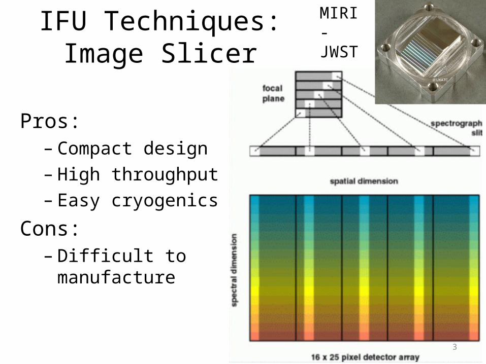
IFU Techniques:Image Slicer
Pros:– Compact design– High throughput– Easy cryogenics
Cons:– Difficult to
manufacture
MIRI - JWST
3

Cross Slice
Alon
g Sl
ice
Sky x
Sky
y
Rectangular Pixels• NIFS has different (x,y) spatial sampling• Along the slice is sampled by the detector• Across the slice is sampled by the slicer• Cross-slice sets spectral PSF - should be sampled on ~2 pixels• Gives rectangular spaxels on the sky
Detector Plane
Sky Plane
4

NIFS
• Near-infrared Integral Field Spectrograph
• Cryogenic slicer design
• Z,J,H,K bands, R~5,000
• One spatial setting:– 3”x3” FoV– 0.1”x0.04” sampling
• Optimized for use with AO
• Science: young stars, exo-planets, solar system, black holes, jets, stellar populations, hi-z galaxies….
5

Typical NIFS Observation• ‘Before’ telluric star
– NGS-AO– Acquire star– Sequence of on/off exposures– Same instrument config as science (inc. e.g. field lens for LGS)
• Science observation– Acquisition– Observation sequence:
• Arc (grating position is not 100% repeatable)• Sequence of on/off exposures
• ‘After’ telluric (if science >~1.5hr)• Daytime calibrations:
– Baseline set:• Flat-lamps (with darks)• ‘Ronchi mask’ flats (with dark)• Darks for the arc
– Darks for science (if sky emission to be used for wavelength calibration)
6
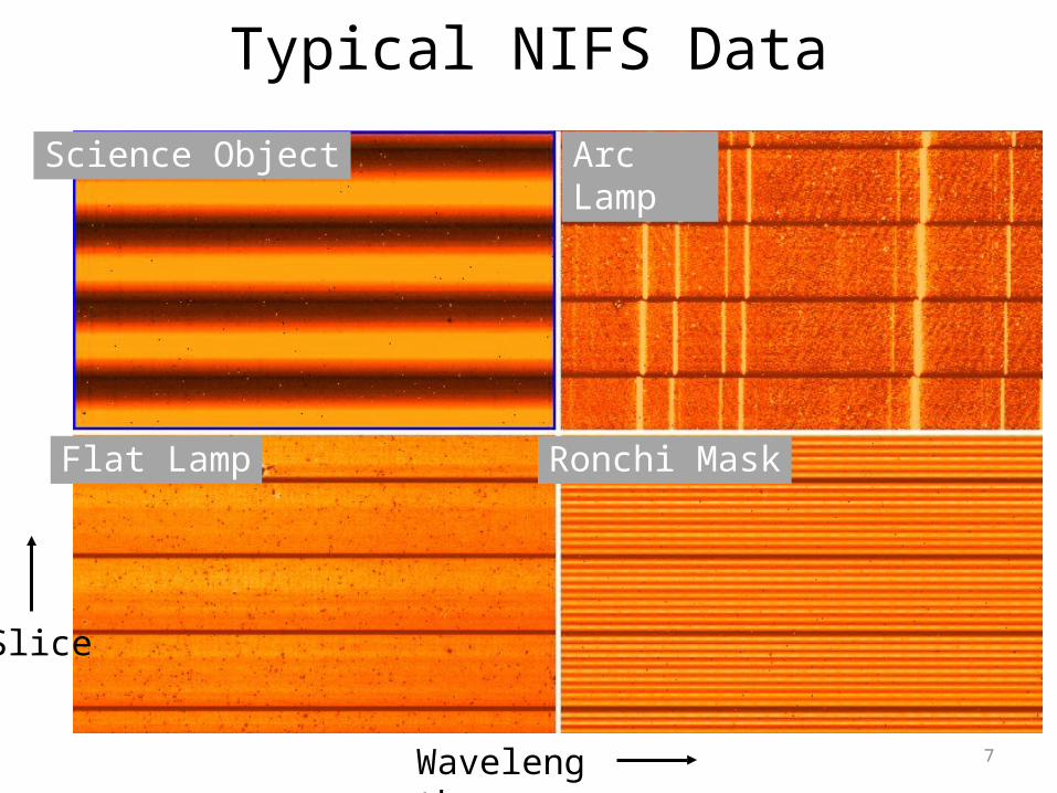
Typical NIFS Data
Science Object Arc Lamp
Flat Lamp Ronchi Mask
Wavelength
Slice
7

Arranging your files - suggestion
Daycals/ - All baseline daytime calibrations
YYYYMMDD/ - cals from different dates
Science/ - All science data
Obj1/ - First science object
YYYYMMDD/ - First obs date (if split over >1 nights)
Config/ - e.g. ‘K’ (if using multiple configs)
Telluric/ - telluric data for this science obs
Merged/ - Merged science and subsequent analysis
Scripts/8

NIFS Reduction: Example scripts
• Three IRAF scripts on the web:– Calibrations– Telluric– Science
• Form the basis of this tutorial• Data set:
– Science object (star)– Telluric correction star– Daytime calibrations
• Update the path and file numbers at the top of each script
• Excellent starting point for basic reduction
9

Lamp Calibrations• Three basic calibrations:
– Flat (DAYCAL)• Correct for transmission and illumination• Locate the spectra on the detector
– Ronchi Mask (DAYCAL)• Spatial distortion
– Arc (NIGHTCAL)• Wavelength calibration
• Each has associated dark frames• May have multiple exposures to co-add• DAYCAL are approx. 1 per observation date• NIGHTCAL are usually once per science
target, but can be common between targets if grating config not changed
10
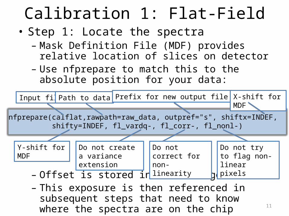
Calibration 1: Flat-Field• Step 1: Locate the spectra
– Mask Definition File (MDF) provides relative location of slices on detector
– Use nfprepare to match this to the absolute position for your data:
– Offset is stored in a new image– This exposure is then referenced in subsequent
steps that need to know where the spectra are on the chip
nfprepare(calflat,rawpath=raw_data, outpref="s", shiftx=INDEF, shifty=INDEF, fl_vardq-, fl_corr-, fl_nonl-)
Input file Path to data Prefix for new output file X-shift for MDF
Y-shift for MDF Do not create a variance extension
Do not correct for non-linearity
Do not try to flag non-linear pixels
11
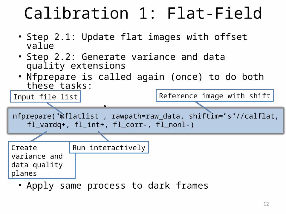
Calibration 1: Flat-Field• Step 2.1: Update flat images with offset value• Step 2.2: Generate variance and data quality
extensions• Nfprepare is called again (once) to do both these
tasks:
• Apply same process to dark frames
nfprepare("@flatlist”, rawpath=raw_data, shiftim="s"//calflat,fl_vardq+, fl_int+, fl_corr-, fl_nonl-)
Input file list Reference image with shift
Create variance and data quality planes
Run interactively
12

Calibration 1: Flat-Field
• Step 2.3: Combine flats and darks using gemcombine:
• Repeat for darks…• Now have 2D images with DQ and VAR extensions.
Ready to go to 3D…
gemcombine("n//@flatlist",output="gn"//calflat, fl_dqpr+, fl_vardq+, masktype="none", logfile="nifs.log”)
Input file list
Propagate DQ Generate VAR/DQ planes
No pixel masking Append outputs to a log file
13

Calibration 1: Flat-Field• Step 3.1: Extract the slices using nsreduce:
• Step 3.2: Create slice-by-slice flat field using nsflat:
– Divides each spectrum (row) in a slice by a fit to the average slice spectrum, with coarse renormalizing
– Also creates a bad pixel mask from the darks
nsreduce("gn"//calflat, fl_nscut+, fl_nsappw+, fl_vardq+,fl_sky-, fl_dark-, fl_flat-, logfile="nifs.log”)
‘cut’ out the slices from the 2D image Apply first order wavelength coordinate system
nsflat("rgn"//calflat, darks="rgn"//flatdark, flatfile="rn"//calflat//"_sflat”, darkfile="rn"//flatdark//"_dark", fl_save_dark+, process="fit”, thr_flo=0.15, thr_fup=1.55, fl_vardq+,logfile="nifs.log")
LOwer and UPper limits for ‘bad’ pixelsOutput flat image
14
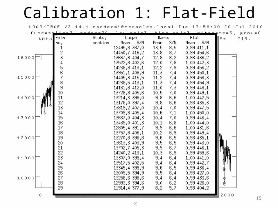
Calibration 1: Flat-Field
15

Calibration 1: Flat-Field• Step 3.3: Renormalize the slices to
account for slice-to-slice variations using nsslitfunction:
– Fits a function in spatial direction to set slice normalization
– Outputs the final flat field, with both spatial and spectral flat information
nsslitfunction("rgn"//calflat, "rn"//calflat//"_flat", flat="rn"//calflat//"_sflat”, dark="rn"//flatdark//"_dark",
combine="median”, order=3, fl_vary-, logfile="nifs.log”)
Final flat-field correction frame
Method to collapse in spectral direction
Order of fit across slices
16
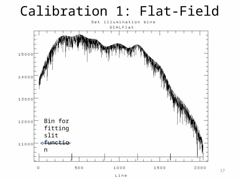
Calibration 1: Flat-Field
Bin for fitting slit function
17

Calibration 1: Flat-Field
Fit to illumination along slice
18

Calibration 2: Wavelength Calibration
• Step 1: Repeat nfprepare, gemcombine and nsreduce -> extracted slices
• Step 2: Correctly identify the arc lines, and determine the dispersion function for each slice– Should run this interactively the first time through to
ensure correct identification of lines and appropriate fit function
– First solution is starting point for subsequent fits– Should robustly determine good solution for
subsequent spectra• Result is a series of files in a ‘database/’ directory
containing the wavelength solutions of each slice
nswavelength("rgn"//arc, coordli=clist, nsum=10, thresho=my_thresh, trace=yes, fwidth=2.0, match=-6, cradius=8.0, fl_inter+, nfound=10, nlost=10, logfile="nifs.log”)
19

Calibration 2: Wavelength Calibration
20

Calibration 2: Wavelength Calibration
21

Calibration 3: Spatial Distortion
• Need to correct for distortions along the slices, and registration between slices
• This is done using the Ronchi mask as a reference
• Analogous to wavelength calibration, but in spatial domain
22
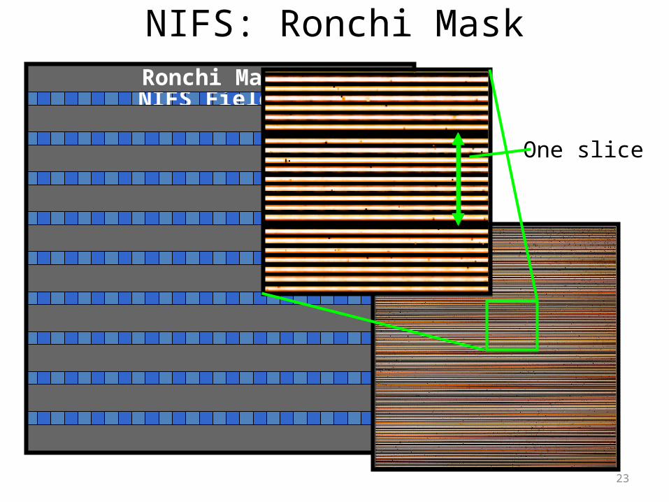
NIFS: Ronchi Mask
NIFS FieldRonchi Mask
One slice
23

NIFS: Ronchi Mask
Simple reconstructed image
Transformation to make lines straight gives geometric correction24

Calibration 3: Spatial Distortion
• Step 1: Repeat nfprepare, gemcombine and nsreduce -> extracted slices
• Step 2: run nfsdist– Reference peaks are very regular, so easy to fall foul
of aliasing when run automatically– Recommend running interactively for each daycal set
• TIP: apply the distortion correction to the Ronchi frame itself, and check its OK
nfsdist("rgn"//ronchiflat, fwidth=6.0, cradius=8.0, glshift=2.8, minsep=6.5, thresh=2000.0, nlost=3, fl_int+, logfile="nifs.log”)
25

Calibration 3: Spatial Distortion
TIP:• If the peaks are shifted, try ‘i’ to initialize, then ‘x’ to fit• Identify with ‘m’ missed peaks if possible
26

Calibration 3: Spatial Distortion
BAD…. GOOD!
Bottom slice is truncated- Slit is extrapolated
27

Lamp Calibrations: Summary
You now have:1. Shift reference file: "s"+calflat 2. Flat field: "rn"+calflat+"_flat" 3. Flat BPM (for DQ plane generation):
"rn"+calflat+"_flat_bpm.pl”4. Wavelength referenced Arc: "wrn"+arc
5. Spatially referenced Ronchi Flat: "rn"+ronchiflat
Notes:– 1-3 are files that you need– 4 & 5 are files with associated files in the ‘database/’ dir– Arcs are likely together with science data
28

Telluric Star
• Similar to science reduction up to a point:– Sky subtraction– Spectra extraction => 3D– Wavelength calibration– Flat fielding
• Then extract 1D spectra, co-add separate observations, and derive the telluric correction spectrum
29

Telluric Star
• Preliminaries:– Copy the calibration files you will need into
telluric directory:– Shift file– Flat– Bad pixel mask (BPM)– Ronchi mask + database dir+files– Arc file + database dir+files
– Make two files listing filenames with (‘object’) and without (‘sky’) star in field
30

Telluric Star
• Step 1.1: Run nfprepare, making use of the shift file and BPM
• Step 1.2: Combine the blank sky frames:– Skies are close in time– Use gemcombine and your list of sky frames
to create a median sky
• Step 1.3: Subtract the combined sky from each object frame with gemarith
31

Telluric Star• Step 2.1: Run nsreduce, this time
including the flat:
• Step 2.2: Replace bad pixels with values interpolated from fitting neighbours
– Uses the Data Quality (QD) plane
nsreduce("sn@telluriclist",outpref="r", flatim=cal_data//"rn"//calflat//"_flat”, fl_nscut+, fl_nsappw-, fl_vardq+, fl_sky-, fl_dark-, fl_flat+, logfile=log_file)
nffixbad("rsn@telluriclist",outpref="b",logfile=log_file)
32

Telluric Star
• Step 3.1: Derive the 2D spectral and spatial transformation for each slice using nsfitcoords– This combines the ‘1D’ dispersion and distortion
solutions derived separately from nswavelength and nsdist into a 2D surface that is linear in wavelength and angular scales
– The parameters of the fitted surface are associated to the object frame via files in the database directory
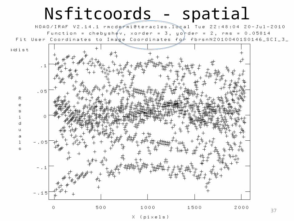
nsfitcoords("brsn@telluriclist", outpref="f", fl_int+, lamptr="wrgn"//arc, sdisttr="rgn"//ronchiflat, lxorder=3, lyorder=3, sxorder=3, syorder=3, logfile=log_file)
33
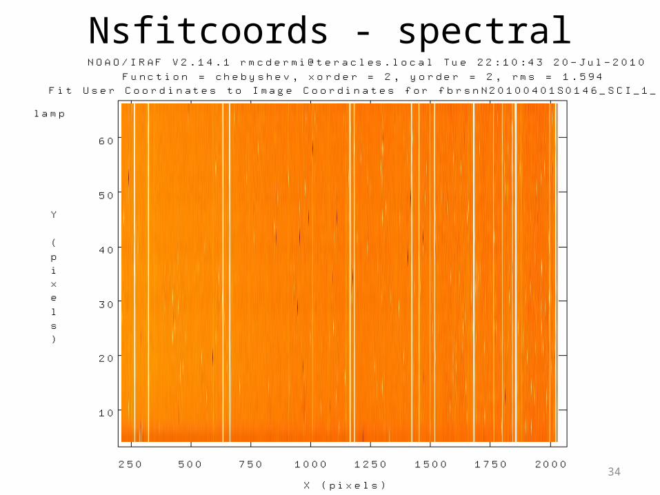
Nsfitcoords - spectral
34

Nsfitcoords - spectral
35
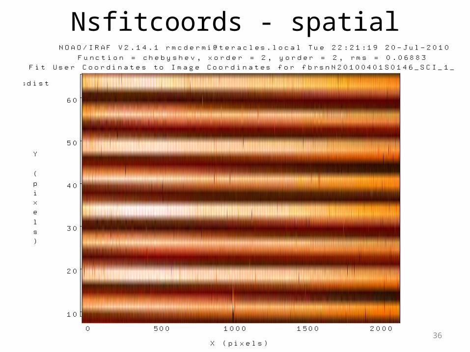
Nsfitcoords - spatial
36
Nsfitcoords - spatial
37
Telluric Star
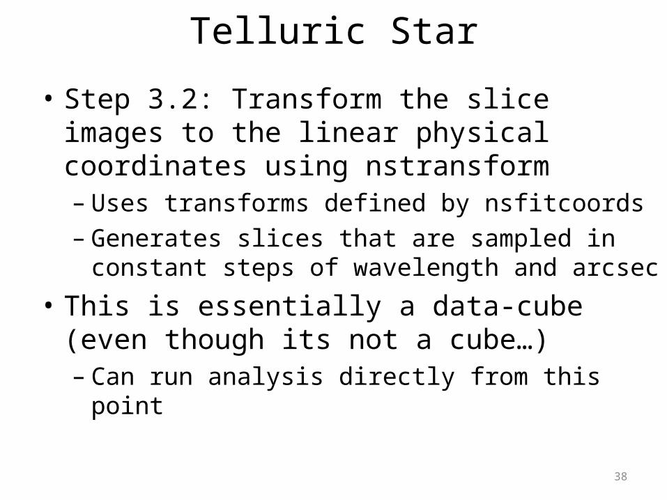
• Step 3.2: Transform the slice images to the linear physical coordinates using nstransform– Uses transforms defined by nsfitcoords– Generates slices that are sampled in constant
steps of wavelength and arcsec
• This is essentially a data-cube (even though its not a cube…)– Can run analysis directly from this point
38
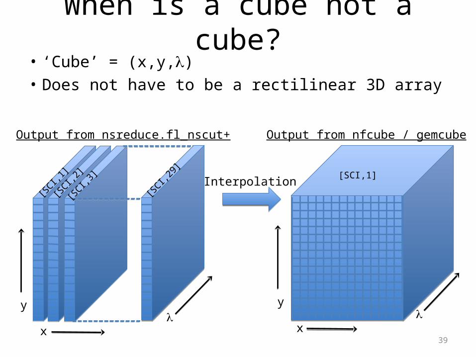
When is a cube not a cube?• ‘Cube’ = (x,y,)
• Does not have to be a rectilinear 3D array
[SCI,1
][S
CI,2]
[SCI,3
]
[SCI,2
9] [SCI,1]
Output from nsreduce.fl_nscut+ Output from nfcube / gemcube
x
y
x
y
Interpolation
39

Telluric Star• Step 4.1: Extract 1D aperture spectra from the data
cube– Use nfextract to define an aperture (radius and centre)
and sum spectra within it– Outputs a 1D spectrum
• Step 4.2: Co-add the 1D spectra using gemcombine
40
Science Data
• Same preliminaries as telluric:– Copy database and arc+Ronchi files– Copy shift file, flat and BPM– Identify sky and object frames
• In addition, we make use of the 1D telluric
• Generally need to combine separate (and dithered) data-cubes
41
Science Data
• Initial steps:– Nfprepare as per telluric– Subtract sky using gemarith
• Usually have one unique sky per object: ABAB• Can have ABA – two science share a sky
– Nsreduce (inc. flat field)– Nffixbad, nsfitcoords, nstransform
• Now have data-cube with linear physical coordinates
42
Science Data: Telluric correction
• Telluric spectrum is not only atmosphere, but also stellar spectrum:– Need to account for stellar absorption features– AND account for black-body continuum
• Needs some ‘by-hand’ steps to prepare the telluric star spectrum– Remove strong stellar features with splot– Remove BB shape with a BB spectrum
43

Science Data: Telluric correction
BB @ 8000K
44

Science Data: Telluric correction
BB @ 8000K
45

Telluric AbsorptionTelluric Absorption
• Alternative approach is to fit a stellar template (Vacca et al. 2003)
• Need good template• Can use solar-type stars, but needs careful treatment…
46

Science Data: Telluric correction• Finally, run nftelluric
– Computes the normalized correction spectrum– Allows for shifts and amplitude scaling– Divides the correction spectrum through the data
Telluric
Science
47
Science Data: Merging
• Now have series of data-cubes:– No dark current or sky (sky-subtracted)– Spatially and spectrally linearized– Bad pixels interpolated over– No instrumental transmission (flat-fielded)– No atmospheric transmission (telluric-corrected)
• Need to combine the data-cubes
48

Two approaches:1. Dithering by non-integer number of spaxels:
• Allows over-sampling, via ‘drizzling’• Resampling introduces correlated noise• Good for fairly bright sources
2. Dither by integer number of spaxels• Allows direct ‘shift and add’ approach• No resampling:- better error characterisation• Assumes accurate (sub-pixel) offsetting• No over-sampling gain• Suitable for ‘deep-field’ applications
Science Data: Merging
Nifcube / gemcube methodNifcube / gemcube method
Imcombine methodImcombine method49
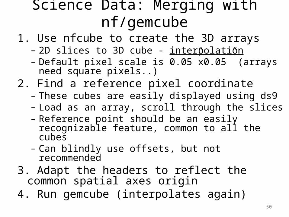
Science Data: Merging with nf/gemcube
1. Use nfcube to create the 3D arrays– 2D slices to 3D cube - interpolation– Default pixel scale is 0.05”x0.05” (arrays need
square pixels..)2. Find a reference pixel coordinate
– These cubes are easily displayed using ds9– Load as an array, scroll through the slices– Reference point should be an easily recognizable
feature, common to all the cubes– Can blindly use offsets, but not recommended
3. Adapt the headers to reflect the common spatial axes origin
4. Run gemcube (interpolates again)50

What headers to change?• Gemcube uses the file WCS to merge overlapping cubes• Need to ‘trick’ the WCS to include your offsets• Following list seemed to work:
– Position of reference source measured on cube plane – different in each cube- CRPIX1 - Reference source (x position in pixels), e.g ‘29’- CRPIX2 - Reference source (y position in pixels), e.g. ‘27.5’
– Approx decimal RA & Dec at reference point – same in all cubes- CRVAL1 - approx. decimal RA of target (same for all cubes)- CRVAL2 - approx. decimal declination of target
– Pixel scale parameters - these are set here to be 0.05 arcsec, but in degrees- CD1_1 = 0.0- CD1_2 = 1.9E-05 - CD2_1 = -4.7e-5 - CD2_2 = 0.0
– Coordinate system info- WAT1_001 = 'wtype=linear axtype=xi’- WAT2_001 = 'wtype=linear axtype=eta’ - CTYPE1 = 'RA---TAN’- CTYPE2 = ‘DEC--TAN'
Hack alert! This is not the best way to proceed! But lets you progress within iraf. Other ideas are welcome!
51

• This approach involves (at least) one superfluous interpolation: nifcube + gemcube both interpolate
• Might be possible to use gemcube directly from pre-transformed data, but wrapper not written (TBD: works on single slices, so can be adapted)
• Nifcube step is convenient for determining reference coordinate, and allows gemcube to combine the frames
• Not ideal, but gives a way to combine your data
Science Data: Merging with nf/gemcube
52

1. Convert files to 3D cubes with nfcube
2. Provide the list of input files, and an ‘offsets’ file of integer shifts to imcombine
Science Data: Merging with imcombine
0 0 0 10 10 0-10 10 0
imcombine(”cat*.fits", output=“Merged”,offset=offsets.dat, logfile=log_file)
offsets.dat x y
53

Other details for merging not covered:– For smoother images / less border effects, individual
cubes should be renormalized to have common flux in overlap regions
– For optimal S/N, spectra should be weighted by the variance when combining
– Even without dithers, long observations will have sub-pixel shifts due to flexure and atmospheric refraction
– To maintain high image quality, keep a reference source common to all fields in the mosaic if possible, and use sub-pixel dithers
Science Data: Merging
54

The End
(….or rather, just the beginning….)
55


