190
NIMBLE User Manual NIMBLE Development Team Version 0.6-12 https://r-nimble.org https://github.com/nimble-dev/nimble

NIMBLE User ManualNIMBLE Development Team
Version 0.6-12
https://r-nimble.orghttps://github.com/nimble-dev/nimble

2

Contents
I Introduction 9
1 Welcome to NIMBLE 11
1.1 What does NIMBLE do? . . . . . . . . . . . . . . . . . . . . . . . . . . . . . . . . . . 11
1.2 How to use this manual . . . . . . . . . . . . . . . . . . . . . . . . . . . . . . . . . . 12
2 Lightning introduction 13
2.1 A brief example . . . . . . . . . . . . . . . . . . . . . . . . . . . . . . . . . . . . . . . 13
2.2 Creating a model . . . . . . . . . . . . . . . . . . . . . . . . . . . . . . . . . . . . . . 13
2.3 Compiling the model . . . . . . . . . . . . . . . . . . . . . . . . . . . . . . . . . . . . 18
2.4 One-line invocation of MCMC . . . . . . . . . . . . . . . . . . . . . . . . . . . . . . . 18
2.5 Creating, compiling and running a basic MCMC configuration . . . . . . . . . . . . . 19
2.6 Customizing the MCMC . . . . . . . . . . . . . . . . . . . . . . . . . . . . . . . . . . 21
2.7 Running MCEM . . . . . . . . . . . . . . . . . . . . . . . . . . . . . . . . . . . . . . 22
2.8 Creating your own functions . . . . . . . . . . . . . . . . . . . . . . . . . . . . . . . . 23
3 More introduction 27
3.1 NIMBLE adopts and extends the BUGS language for specifying models . . . . . . . 27
3.2 nimbleFunctions for writing algorithms . . . . . . . . . . . . . . . . . . . . . . . . . . 28
3.3 The NIMBLE algorithm library . . . . . . . . . . . . . . . . . . . . . . . . . . . . . . 29
4 Installing NIMBLE 31
4.1 Requirements to run NIMBLE . . . . . . . . . . . . . . . . . . . . . . . . . . . . . . 31
4.2 Installing a C++ compiler for NIMBLE to use . . . . . . . . . . . . . . . . . . . . . 31
4.2.1 OS X . . . . . . . . . . . . . . . . . . . . . . . . . . . . . . . . . . . . . . . . 32
4.2.2 Linux . . . . . . . . . . . . . . . . . . . . . . . . . . . . . . . . . . . . . . . . 32
4.2.3 Windows . . . . . . . . . . . . . . . . . . . . . . . . . . . . . . . . . . . . . . 32
4.3 Installing the NIMBLE package . . . . . . . . . . . . . . . . . . . . . . . . . . . . . . 32
3
4 CONTENTS
4.3.1 Problems with installation . . . . . . . . . . . . . . . . . . . . . . . . . . . . . 334.4 Customizing your installation . . . . . . . . . . . . . . . . . . . . . . . . . . . . . . . 33
4.4.1 Using your own copy of Eigen . . . . . . . . . . . . . . . . . . . . . . . . . . . 334.4.2 Using libnimble . . . . . . . . . . . . . . . . . . . . . . . . . . . . . . . . . . . 334.4.3 BLAS and LAPACK . . . . . . . . . . . . . . . . . . . . . . . . . . . . . . . . 344.4.4 Customizing compilation of the NIMBLE-generated C++ . . . . . . . . . . . 34
II Models in NIMBLE 35
5 Writing models in NIMBLE’s dialect of BUGS 375.1 Comparison to BUGS dialects supported by WinBUGS, OpenBUGS and JAGS . . . 37
5.1.1 Supported features of BUGS and JAGS . . . . . . . . . . . . . . . . . . . . . 375.1.2 NIMBLE’s Extensions to BUGS and JAGS . . . . . . . . . . . . . . . . . . . 375.1.3 Not-yet-supported features of BUGS and JAGS . . . . . . . . . . . . . . . . . 38
5.2 Writing models . . . . . . . . . . . . . . . . . . . . . . . . . . . . . . . . . . . . . . . 385.2.1 Declaring stochastic and deterministic nodes . . . . . . . . . . . . . . . . . . 395.2.2 More kinds of BUGS declarations . . . . . . . . . . . . . . . . . . . . . . . . . 415.2.3 Vectorized versus scalar declarations . . . . . . . . . . . . . . . . . . . . . . . 435.2.4 Available distributions . . . . . . . . . . . . . . . . . . . . . . . . . . . . . . . 445.2.5 Available BUGS language functions . . . . . . . . . . . . . . . . . . . . . . . . 485.2.6 Available link functions . . . . . . . . . . . . . . . . . . . . . . . . . . . . . . 505.2.7 Truncation, censoring, and constraints . . . . . . . . . . . . . . . . . . . . . . 51
6 Building and using models 556.1 Creating model objects . . . . . . . . . . . . . . . . . . . . . . . . . . . . . . . . . . . 55
6.1.1 Using nimbleModel to create a model . . . . . . . . . . . . . . . . . . . . . . . 556.1.2 Creating a model from standard BUGS and JAGS input files . . . . . . . . . 596.1.3 Making multiple instances from the same model definition . . . . . . . . . . . 60
6.2 NIMBLE models are objects you can query and manipulate . . . . . . . . . . . . . . 616.2.1 What are variables and nodes? . . . . . . . . . . . . . . . . . . . . . . . . . . 616.2.2 Determining the nodes and variables in a model . . . . . . . . . . . . . . . . 616.2.3 Accessing nodes . . . . . . . . . . . . . . . . . . . . . . . . . . . . . . . . . . . 626.2.4 How nodes are named . . . . . . . . . . . . . . . . . . . . . . . . . . . . . . . 646.2.5 Why use node names? . . . . . . . . . . . . . . . . . . . . . . . . . . . . . . . 646.2.6 Checking if a node holds data . . . . . . . . . . . . . . . . . . . . . . . . . . . 64
CONTENTS 5
III Algorithms in NIMBLE 67
7 MCMC 69
7.1 One-line invocation of MCMC: nimbleMCMC . . . . . . . . . . . . . . . . . . . . . . 70
7.2 The MCMC configuration . . . . . . . . . . . . . . . . . . . . . . . . . . . . . . . . . 71
7.2.1 Default MCMC configuration . . . . . . . . . . . . . . . . . . . . . . . . . . . 72
7.2.2 Customizing the MCMC configuration . . . . . . . . . . . . . . . . . . . . . . 73
7.3 Building and compiling the MCMC . . . . . . . . . . . . . . . . . . . . . . . . . . . . 79
7.4 User-friendly execution of MCMC algorithms: runMCMC . . . . . . . . . . . . . . . 80
7.5 Running the MCMC . . . . . . . . . . . . . . . . . . . . . . . . . . . . . . . . . . . . 81
7.5.1 Measuring sampler computation times: getTimes . . . . . . . . . . . . . . . 82
7.6 Extracting MCMC samples . . . . . . . . . . . . . . . . . . . . . . . . . . . . . . . . 82
7.7 Calculating WAIC . . . . . . . . . . . . . . . . . . . . . . . . . . . . . . . . . . . . . 83
7.8 k-fold cross-validation . . . . . . . . . . . . . . . . . . . . . . . . . . . . . . . . . . . 83
7.9 Samplers provided with NIMBLE . . . . . . . . . . . . . . . . . . . . . . . . . . . . . 83
7.9.1 Conjugate (‘Gibbs’) samplers . . . . . . . . . . . . . . . . . . . . . . . . . . . 83
7.9.2 Customized log-likelihood evaluations: RW_llFunction sampler . . . . . . . . 84
7.9.3 Particle MCMC sampler . . . . . . . . . . . . . . . . . . . . . . . . . . . . . . 85
7.10 Detailed MCMC example: litters . . . . . . . . . . . . . . . . . . . . . . . . . . . . . 86
7.11 Comparing different MCMCs with MCMCsuite and compareMCMCs . . . . . . . . . 88
7.11.1 MCMC Suite example: litters . . . . . . . . . . . . . . . . . . . . . . . . . . . 88
7.11.2 MCMC Suite outputs . . . . . . . . . . . . . . . . . . . . . . . . . . . . . . . 89
7.11.3 Customizing MCMC Suite . . . . . . . . . . . . . . . . . . . . . . . . . . . . . 90
8 Sequential Monte Carlo and MCEM 93
8.1 Particle Filters / Sequential Monte Carlo . . . . . . . . . . . . . . . . . . . . . . . . 93
8.1.1 Filtering Algorithms . . . . . . . . . . . . . . . . . . . . . . . . . . . . . . . . 93
8.1.2 Particle MCMC (PMCMC) . . . . . . . . . . . . . . . . . . . . . . . . . . . . 96
8.2 Monte Carlo Expectation Maximization (MCEM) . . . . . . . . . . . . . . . . . . . . 97
8.2.1 Estimating the Asymptotic Covariance From MCEM . . . . . . . . . . . . . . 100
9 Spatial models 101
9.1 Intrinsic Gaussian CAR model: dcar_normal . . . . . . . . . . . . . . . . . . . . . . 101
9.1.1 Specification and density . . . . . . . . . . . . . . . . . . . . . . . . . . . . . 101
9.1.2 Example . . . . . . . . . . . . . . . . . . . . . . . . . . . . . . . . . . . . . . . 103

6 CONTENTS
9.2 Proper Gaussian CAR model: dcar_proper . . . . . . . . . . . . . . . . . . . . . . . 104
9.2.1 Specification and density . . . . . . . . . . . . . . . . . . . . . . . . . . . . . 104
9.2.2 Example . . . . . . . . . . . . . . . . . . . . . . . . . . . . . . . . . . . . . . . 105
9.3 MCMC Sampling of CAR models . . . . . . . . . . . . . . . . . . . . . . . . . . . . . 107
9.3.1 Initial values . . . . . . . . . . . . . . . . . . . . . . . . . . . . . . . . . . . . 107
9.3.2 Zero-neighbor regions . . . . . . . . . . . . . . . . . . . . . . . . . . . . . . . 107
9.3.3 Zero-mean constraint . . . . . . . . . . . . . . . . . . . . . . . . . . . . . . . . 108
10 Bayesian nonparametric models 109
10.1 Bayesian nonparametric mixture models . . . . . . . . . . . . . . . . . . . . . . . . . 109
10.2 Chinese Restaurant Process model . . . . . . . . . . . . . . . . . . . . . . . . . . . . 110
10.2.1 Specification and density . . . . . . . . . . . . . . . . . . . . . . . . . . . . . 110
10.2.2 Example . . . . . . . . . . . . . . . . . . . . . . . . . . . . . . . . . . . . . . . 111
10.3 Stick-breaking model . . . . . . . . . . . . . . . . . . . . . . . . . . . . . . . . . . . . 112
10.3.1 Specification and function . . . . . . . . . . . . . . . . . . . . . . . . . . . . . 112
10.3.2 Example . . . . . . . . . . . . . . . . . . . . . . . . . . . . . . . . . . . . . . . 113
10.4 MCMC sampling of BNP models . . . . . . . . . . . . . . . . . . . . . . . . . . . . . 114
10.4.1 Sampling CRP models . . . . . . . . . . . . . . . . . . . . . . . . . . . . . . . 114
10.4.2 Sampling stick-breaking models . . . . . . . . . . . . . . . . . . . . . . . . . . 115
IV Programming with NIMBLE 117
11 Writing simple nimbleFunctions 121
11.1 Introduction to simple nimbleFunctions . . . . . . . . . . . . . . . . . . . . . . . . . 121
11.2 R functions (or variants) implemented in NIMBLE . . . . . . . . . . . . . . . . . . . 122
11.2.1 Finding help for NIMBLE’s versions of R functions . . . . . . . . . . . . . . . 122
11.2.2 Basic operations . . . . . . . . . . . . . . . . . . . . . . . . . . . . . . . . . . 122
11.2.3 Math and linear algebra . . . . . . . . . . . . . . . . . . . . . . . . . . . . . . 124
11.2.4 Distribution functions . . . . . . . . . . . . . . . . . . . . . . . . . . . . . . . 126
11.2.5 Flow control: if-then-else, for, while, and stop . . . . . . . . . . . . . . . . . . 127
11.2.6 print and cat . . . . . . . . . . . . . . . . . . . . . . . . . . . . . . . . . . . . 128
11.2.7 Checking for user interrupts: checkInterrupt . . . . . . . . . . . . . . . . . . . 128
11.2.8 Optimization: optim and nimOptim . . . . . . . . . . . . . . . . . . . . . . . 128
11.2.9 ‘nim’ synonyms for some functions . . . . . . . . . . . . . . . . . . . . . . . . 128

CONTENTS 7
11.3 How NIMBLE handles types of variables . . . . . . . . . . . . . . . . . . . . . . . . . 12911.3.1 nimbleList data structures . . . . . . . . . . . . . . . . . . . . . . . . . . . . . 12911.3.2 How numeric types work . . . . . . . . . . . . . . . . . . . . . . . . . . . . . . 129
11.4 Declaring argument and return types . . . . . . . . . . . . . . . . . . . . . . . . . . . 13311.5 Compiled nimbleFunctions pass arguments by reference . . . . . . . . . . . . . . . . 13311.6 Calling external compiled code . . . . . . . . . . . . . . . . . . . . . . . . . . . . . . 13311.7 Calling uncompiled R functions from compiled nimbleFunctions . . . . . . . . . . . . 134
12 Creating user-defined BUGS distributions and functions 13512.1 User-defined functions . . . . . . . . . . . . . . . . . . . . . . . . . . . . . . . . . . . 13512.2 User-defined distributions . . . . . . . . . . . . . . . . . . . . . . . . . . . . . . . . . 136
12.2.1 Using registerDistributions for alternative parameterizations and providingother information . . . . . . . . . . . . . . . . . . . . . . . . . . . . . . . . . . 139
13 Working with NIMBLE models 14113.1 The variables and nodes in a NIMBLE model . . . . . . . . . . . . . . . . . . . . . . 141
13.1.1 Determining the nodes in a model . . . . . . . . . . . . . . . . . . . . . . . . 14113.1.2 Understanding lifted nodes . . . . . . . . . . . . . . . . . . . . . . . . . . . . 14313.1.3 Determining dependencies in a model . . . . . . . . . . . . . . . . . . . . . . 143
13.2 Accessing information about nodes and variables . . . . . . . . . . . . . . . . . . . . 14513.2.1 Getting distributional information about a node . . . . . . . . . . . . . . . . 14513.2.2 Getting information about a distribution . . . . . . . . . . . . . . . . . . . . 14613.2.3 Getting distribution parameter values for a node . . . . . . . . . . . . . . . . 14613.2.4 Getting distribution bounds for a node . . . . . . . . . . . . . . . . . . . . . . 147
13.3 Carrying out model calculations . . . . . . . . . . . . . . . . . . . . . . . . . . . . . . 14813.3.1 Core model operations: calculation and simulation . . . . . . . . . . . . . . . 14813.3.2 Pre-defined nimbleFunctions for operating on model nodes: simNodes, calc-
Nodes, and getLogProbNodes . . . . . . . . . . . . . . . . . . . . . . . . . . . . 15013.3.3 Accessing log probabilities via logProb variables . . . . . . . . . . . . . . . . . 152
14 Data structures in NIMBLE 15514.1 The modelValues data structure . . . . . . . . . . . . . . . . . . . . . . . . . . . . . 155
14.1.1 Creating modelValues objects . . . . . . . . . . . . . . . . . . . . . . . . . . . 15514.1.2 Accessing contents of modelValues . . . . . . . . . . . . . . . . . . . . . . . . 157
14.2 The nimbleList data structure . . . . . . . . . . . . . . . . . . . . . . . . . . . . . . . 16114.2.1 Using eigen and svd in nimbleFunctions . . . . . . . . . . . . . . . . . . . . . 163

8 CONTENTS
15 Writing nimbleFunctions to interact with models 167
15.1 Overview . . . . . . . . . . . . . . . . . . . . . . . . . . . . . . . . . . . . . . . . . . 167
15.2 Using and compiling nimbleFunctions . . . . . . . . . . . . . . . . . . . . . . . . . . 169
15.3 Writing setup code . . . . . . . . . . . . . . . . . . . . . . . . . . . . . . . . . . . . . 170
15.3.1 Useful tools for setup functions . . . . . . . . . . . . . . . . . . . . . . . . . . 170
15.3.2 Accessing and modifying numeric values from setup . . . . . . . . . . . . . . 170
15.3.3 Determining numeric types in nimbleFunctions . . . . . . . . . . . . . . . . . 171
15.3.4 Control of setup outputs . . . . . . . . . . . . . . . . . . . . . . . . . . . . . . 171
15.4 Writing run code . . . . . . . . . . . . . . . . . . . . . . . . . . . . . . . . . . . . . . 171
15.4.1 Driving models: calculate, calculateDiff, simulate, getLogProb . . . . . . . . . 172
15.4.2 Getting and setting variable and node values . . . . . . . . . . . . . . . . . . 172
15.4.3 Getting parameter values and node bounds . . . . . . . . . . . . . . . . . . . 174
15.4.4 Using modelValues objects . . . . . . . . . . . . . . . . . . . . . . . . . . . . 174
15.4.5 Using model variables and modelValues in expressions . . . . . . . . . . . . . 178
15.4.6 Including other methods in a nimbleFunction . . . . . . . . . . . . . . . . . . 179
15.4.7 Using other nimbleFunctions . . . . . . . . . . . . . . . . . . . . . . . . . . . 180
15.4.8 Virtual nimbleFunctions and nimbleFunctionLists . . . . . . . . . . . . . . . . 181
15.4.9 Character objects . . . . . . . . . . . . . . . . . . . . . . . . . . . . . . . . . . 183
15.4.10 User-defined data structures . . . . . . . . . . . . . . . . . . . . . . . . . . . . 183
15.5 Example: writing user-defined samplers to extend NIMBLE’s MCMC engine . . . . 185
15.6 Copying nimbleFunctions (and NIMBLE models) . . . . . . . . . . . . . . . . . . . . 186
15.7 Debugging nimbleFunctions . . . . . . . . . . . . . . . . . . . . . . . . . . . . . . . . 187
15.8 Timing nimbleFunctions with run.time . . . . . . . . . . . . . . . . . . . . . . . . . . 187
15.9 Reducing memory usage . . . . . . . . . . . . . . . . . . . . . . . . . . . . . . . . . . 188

Part I
Introduction
9


Chapter 1
Welcome to NIMBLE
NIMBLE is a system for building and sharing analysis methods for statistical models from R, espe-cially for hierarchical models and computationally-intensive methods. While NIMBLE is embeddedin R, it goes beyond R by supporting separate programming of models and algorithms along withcompilation for fast execution.
As of version 0.6-12, NIMBLE has been around for a while and is reasonably stable, but we havea lot of plans to expand and improve it. The algorithm library provides MCMC with a lot ofuser control and ability to write new samplers easily. Other algorithms include particle filtering(sequential Monte Carlo) and Monte Carlo Expectation Maximization (MCEM).
But NIMBLE is about much more than providing an algorithm library. It provides a language forwriting model-generic algorithms. We hope you will program in NIMBLE and make an R packageproviding your method. Of course, NIMBLE is open source, so we also hope you’ll contribute toits development.
Please join the mailing lists (see R-nimble.org/more/issues-and-groups) and help improve NIMBLEby telling us what you want to do with it, what you like, and what could be better. We have alot of ideas for how to improve it, but we want your help and ideas too. You can also follow andcontribute to developer discussions on the wiki of our GitHub repository.
If you use NIMBLE in your work, please cite us, as this helps justify past and future funding forthe development of NIMBLE. For more information, please call citation('nimble') in R.
1.1 What does NIMBLE do?
NIMBLE makes it easier to program statistical algorithms that will run efficiently and work onmany different models from R.
You can think of NIMBLE as comprising four pieces:
1. A system for writing statistical models flexibly, which is an extension of the BUGS language1.2. A library of algorithms such as MCMC.1See Chapter 5 for information about NIMBLE’s version of BUGS.
11

12 CHAPTER 1. WELCOME TO NIMBLE
3. A language, called NIMBLE, embedded within and similar in style to R, for writing algorithmsthat operate on models written in BUGS.
4. A compiler that generates C++ for your models and algorithms, compiles that C++, andlets you use it seamlessly from R without knowing anything about C++.
NIMBLE stands for Numerical Inference for statistical Models for Bayesian and Likelihood Esti-mation.
Although NIMBLE was motivated by algorithms for hierarchical statistical models, it’s useful forother goals too. You could use it for simpler models. And since NIMBLE can automaticallycompile R-like functions into C++ that use the Eigen library for fast linear algebra, you can use itto program fast numerical functions without any model involved2.
One of the beauties of R is that many of the high-level analysis functions are themselves written inR, so it is easy to see their code and modify them. The same is true for NIMBLE: the algorithmsare themselves written in the NIMBLE language.
1.2 How to use this manual
We suggest everyone start with the Lightning Introduction in Chapter 2.
Then, if you want to jump into using NIMBLE’s algorithms without learning about NIMBLE’sprogramming system, go to Part II to learn how to build your model and Part III to learn how toapply NIMBLE’s built-in algorithms to your model.
If you want to learn about NIMBLE programming (nimbleFunctions), go to Part IV. This teacheshow to program user-defined function or distributions to use in BUGS code, compile your R codefor faster operations, and write algorithms with NIMBLE. These algorithms could be specific algo-rithms for your particular model (such as a user-defined MCMC sampler for a parameter in yourmodel) or general algorithms you can distribute to others. In fact the algorithms provided as partof NIMBLE and described in Part III are written as nimbleFunctions.
2The packages Rcpp and RcppEigen provide different ways of connecting C++, the Eigen library and R. In thosepackages you program directly in C++, while in NIMBLE you program in R in a nimbleFunction and the NIMBLEcompiler turns it into C++.

Chapter 2
Lightning introduction
2.1 A brief example
Here we’ll give a simple example of building a model and running some algorithms on the model,as well as creating our own user-specified algorithm. The goal is to give you a sense for what onecan do in the system. Later sections will provide more detail.
We’ll use the pump model example from BUGS1. We could load the model from the standard BUGSexample file formats (Section 6.1.2), but instead we’ll show how to enter it directly in R.
In this ‘lightning introduction’ we will:
1. Create the model for the pump example.2. Compile the model.3. Create a basic MCMC configuration for the pump model.4. Compile and run the MCMC5. Customize the MCMC configuration and compile and run that.6. Create, compile and run a Monte Carlo Expectation Maximization (MCEM) algorithm, which
illustrates some of the flexibility NIMBLE provides to combine R and NIMBLE.7. Write a short nimbleFunction to generate simulations from designated nodes of any model.
2.2 Creating a model
First we define the model code, its constants, data, and initial values for MCMC.
pumpCode <- nimbleCode({for (i in 1:N){
theta[i] ~ dgamma(alpha,beta)lambda[i] <- theta[i]*t[i]x[i] ~ dpois(lambda[i])
}alpha ~ dexp(1.0)
1The data set describes failure rates of some pumps.
13

14 CHAPTER 2. LIGHTNING INTRODUCTION
beta ~ dgamma(0.1,1.0)})
pumpConsts <- list(N = 10,t = c(94.3, 15.7, 62.9, 126, 5.24,
31.4, 1.05, 1.05, 2.1, 10.5))
pumpData <- list(x = c(5, 1, 5, 14, 3, 19, 1, 1, 4, 22))
pumpInits <- list(alpha = 1, beta = 1,theta = rep(0.1, pumpConsts$N))
Here x[i] is the number of failures recorded during a time duration of length t[i] for the ith
pump. theta[i] is a failure rate, and the goal is estimate parameters alpha and beta. Now let’screate the model and look at some of its nodes.
pump <- nimbleModel(code = pumpCode, name = "pump", constants = pumpConsts,data = pumpData, inits = pumpInits)
pump$getNodeNames()
## [1] "alpha" "beta" "lifted_d1_over_beta"## [4] "theta[1]" "theta[2]" "theta[3]"## [7] "theta[4]" "theta[5]" "theta[6]"## [10] "theta[7]" "theta[8]" "theta[9]"## [13] "theta[10]" "lambda[1]" "lambda[2]"## [16] "lambda[3]" "lambda[4]" "lambda[5]"## [19] "lambda[6]" "lambda[7]" "lambda[8]"## [22] "lambda[9]" "lambda[10]" "x[1]"## [25] "x[2]" "x[3]" "x[4]"## [28] "x[5]" "x[6]" "x[7]"## [31] "x[8]" "x[9]" "x[10]"
pump$x
## [1] 5 1 5 14 3 19 1 1 4 22
pump$logProb_x
## [1] -2.998011 -1.118924 -1.882686 -2.319466 -4.254550 -20.739651## [7] -2.358795 -2.358795 -9.630645 -48.447798
pump$alpha
## [1] 1

2.2. CREATING A MODEL 15
pump$theta
## [1] 0.1 0.1 0.1 0.1 0.1 0.1 0.1 0.1 0.1 0.1
pump$lambda
## [1] 9.430 1.570 6.290 12.600 0.524 3.140 0.105 0.105 0.210 1.050
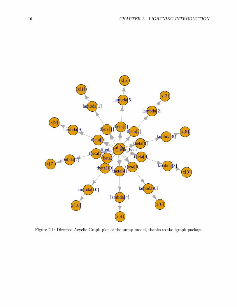
Notice that in the list of nodes, NIMBLE has introduced a new node, lifted_d1_over_beta. Wecall this a ‘lifted’ node. Like R, NIMBLE allows alternative parameterizations, such as the scale orrate parameterization of the gamma distribution. Choice of parameterization can generate a liftednode, as can using a link function or a distribution argument that is an expression. It’s helpful toknow why they exist, but you shouldn’t need to worry about them.
Thanks to the plotting capabilities of the igraph package that NIMBLE uses to represent thedirected acyclic graph, we can plot the model (Figure 2.1).
pump$plotGraph()
You are in control of the model. By default, nimbleModel does its best to initialize a model, butlet’s say you want to re-initialize theta. To simulate from the prior for theta (overwriting theinitial values previously in the model) we first need to be sure the parent nodes of all theta[i]nodes are fully initialized, including any non-stochastic nodes such as lifted nodes. We then usethe simulate function to simulate from the distribution for theta. Finally we use the calculatefunction to calculate the dependencies of theta, namely lambda and the log probabilities of x toensure all parts of the model are up to date. First we show how to use the model’s getDependenciesmethod to query information about its graph.
# Show all dependencies of alpha and beta terminating in stochastic nodespump$getDependencies(c("alpha", "beta"))
## [1] "alpha" "beta" "lifted_d1_over_beta"## [4] "theta[1]" "theta[2]" "theta[3]"## [7] "theta[4]" "theta[5]" "theta[6]"## [10] "theta[7]" "theta[8]" "theta[9]"## [13] "theta[10]"
# Now show only the deterministic dependenciespump$getDependencies(c("alpha", "beta"), determOnly = TRUE)
## [1] "lifted_d1_over_beta"
16 CHAPTER 2. LIGHTNING INTRODUCTION
alpha
beta
lifted_d1_over_beta
theta[1] theta[2]
theta[3]
theta[4]
theta[5]
theta[6]
theta[7]
theta[8]theta[9]
theta[10]
lambda[1]lambda[2]
lambda[3]
lambda[4]
lambda[5]
lambda[6]
lambda[7]
lambda[8]
lambda[9]
lambda[10]
x[1]
x[2]
x[3]
x[4]
x[5]
x[6]
x[7]
x[8]
x[9]
x[10]
Figure 2.1: Directed Acyclic Graph plot of the pump model, thanks to the igraph package

2.2. CREATING A MODEL 17
# Check that the lifted node was initialized.pump[["lifted_d1_over_beta"]] # It was.
## [1] 1
# Now let's simulate new theta valuesset.seed(1) # This makes the simulations here reproduciblepump$simulate("theta")pump$theta # the new theta values
## [1] 0.15514136 1.88240160 1.80451250 0.83617765 1.22254365 1.15835525## [7] 0.99001994 0.30737332 0.09461909 0.15720154
# lambda and logProb_x haven't been re-calculated yetpump$lambda # these are the same values as above
## [1] 9.430 1.570 6.290 12.600 0.524 3.140 0.105 0.105 0.210 1.050
pump$logProb_x
## [1] -2.998011 -1.118924 -1.882686 -2.319466 -4.254550 -20.739651## [7] -2.358795 -2.358795 -9.630645 -48.447798
pump$getLogProb("x") # The sum of logProb_x
## [1] -96.10932
pump$calculate(pump$getDependencies(c("theta")))
## [1] -262.204
pump$lambda # Now they have.
## [1] 14.6298299 29.5537051 113.5038360 105.3583839 6.4061287## [6] 36.3723548 1.0395209 0.3227420 0.1987001 1.6506161
pump$logProb_x
## [1] -6.002009 -26.167496 -94.632145 -65.346457 -2.626123 -7.429868## [7] -1.000761 -1.453644 -9.840589 -39.096527
Notice that the first getDependencies call returned dependencies from alpha and beta down to thenext stochastic nodes in the model. The second call requested only deterministic dependencies. Thecall to pump$simulate("theta") expands "theta" to include all nodes in theta. After simulatinginto theta, we can see that lambda and the log probabilities of x still reflect the old values of theta,so we calculate them and then see that they have been updated.

18 CHAPTER 2. LIGHTNING INTRODUCTION
2.3 Compiling the model
Next we compile the model, which means generating C++ code, compiling that code, and loadingit back into R with an object that can be used just like the uncompiled model. The values inthe compiled model will be initialized from those of the original model in R, but the original andcompiled models are distinct objects so any subsequent changes in one will not be reflected in theother.
Cpump <- compileNimble(pump)Cpump$theta
## [1] 0.15514136 1.88240160 1.80451250 0.83617765 1.22254365 1.15835525## [7] 0.99001994 0.30737332 0.09461909 0.15720154
Note that the compiled model is used when running any NIMBLE algorithms via C++, so themodel needs to be compiled before (or at the same time as) any compilation of algorithms, such asthe compilation of the MCMC done in the next section.
2.4 One-line invocation of MCMC
The most direct approach to invoking NIMBLE’s MCMC engine is using the nimbleMCMC function.This function would generally take the code, data, constants, and initial values as input, but it canalso accept the (compiled or uncompiled) model object as an argument. It provides a variety ofoptions for executing and controlling multiple chains of NIMBLE’s default MCMC algorithm, andreturning posterior samples, posterior summary statistics, and/or WAIC values.
For example, to execute two MCMC chains of 10,000 samples each, and return samples, summarystatistics, and WAIC values:
mcmc.out <- nimbleMCMC(code = pumpCode, constants = pumpConsts,data = pumpData, inits = pumpInits,nchains = 2, niter = 10000,summary = TRUE, WAIC = TRUE)
names(mcmc.out)
## [1] "samples" "summary" "WAIC"
mcmc.out$summary
## $chain1## Mean Median St.Dev. 95%CI_low 95%CI_upp## alpha 0.6980435 0.6583506 0.2703768 0.2878982 1.314046## beta 0.9286260 0.8215685 0.5496913 0.1836991 2.287270#### $chain2
2.5. CREATING, COMPILING AND RUNNING A BASIC MCMC CONFIGURATION 19
## Mean Median St.Dev. 95%CI_low 95%CI_upp## alpha 0.6910196 0.6580365 0.2654838 0.2771956 1.285815## beta 0.9162727 0.8143443 0.5375082 0.1857723 2.270243#### $all.chains## Mean Median St.Dev. 95%CI_low 95%CI_upp## alpha 0.6945316 0.6580365 0.2679578 0.2832985 1.299932## beta 0.9224494 0.8182816 0.5436554 0.1854908 2.278544
mcmc.out$waic
## NULL
See Section 7.1 or help(nimbleMCMC) for more details about using nimbleMCMC.
2.5 Creating, compiling and running a basic MCMC configuration
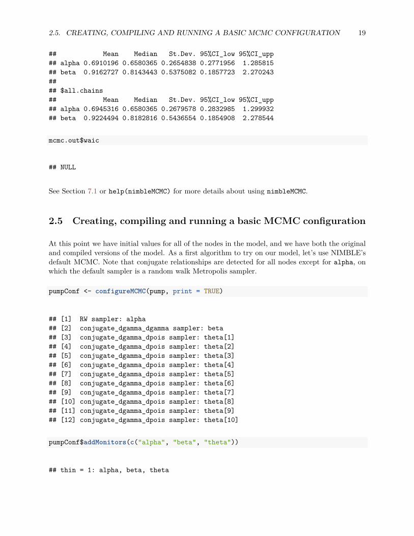
At this point we have initial values for all of the nodes in the model, and we have both the originaland compiled versions of the model. As a first algorithm to try on our model, let’s use NIMBLE’sdefault MCMC. Note that conjugate relationships are detected for all nodes except for alpha, onwhich the default sampler is a random walk Metropolis sampler.
pumpConf <- configureMCMC(pump, print = TRUE)
## [1] RW sampler: alpha## [2] conjugate_dgamma_dgamma sampler: beta## [3] conjugate_dgamma_dpois sampler: theta[1]## [4] conjugate_dgamma_dpois sampler: theta[2]## [5] conjugate_dgamma_dpois sampler: theta[3]## [6] conjugate_dgamma_dpois sampler: theta[4]## [7] conjugate_dgamma_dpois sampler: theta[5]## [8] conjugate_dgamma_dpois sampler: theta[6]## [9] conjugate_dgamma_dpois sampler: theta[7]## [10] conjugate_dgamma_dpois sampler: theta[8]## [11] conjugate_dgamma_dpois sampler: theta[9]## [12] conjugate_dgamma_dpois sampler: theta[10]
pumpConf$addMonitors(c("alpha", "beta", "theta"))
## thin = 1: alpha, beta, theta

20 CHAPTER 2. LIGHTNING INTRODUCTION
pumpMCMC <- buildMCMC(pumpConf)CpumpMCMC <- compileNimble(pumpMCMC, project = pump)
niter <- 1000set.seed(1)samples <- runMCMC(CpumpMCMC, niter = niter)
par(mfrow = c(1, 4), mai = c(.6, .4, .1, .2))plot(samples[ , "alpha"], type = "l", xlab = "iteration",
ylab = expression(alpha))plot(samples[ , "beta"], type = "l", xlab = "iteration",
ylab = expression(beta))plot(samples[ , "alpha"], samples[ , "beta"], xlab = expression(alpha),
ylab = expression(beta))plot(samples[ , "theta[1]"], type = "l", xlab = "iteration",
ylab = expression(theta[1]))
0 400 800
0.5
1.0
1.5
iteration
α
0 400 800
0.0
0.5
1.0
1.5
2.0
2.5
3.0
iteration
β
0.5 1.0 1.5
0.0
0.5
1.0
1.5
2.0
2.5
3.0
α
β
0 400 800
0.02
0.06
0.10
0.14
iteration
θ 1
acf(samples[, "alpha"]) # plot autocorrelation of alpha sampleacf(samples[, "beta"]) # plot autocorrelation of beta sample
0 5 15 25
0.0
0.2
0.4
0.6
0.8
1.0
Lag
AC
F
0 5 15 25
0.0
0.2
0.4
0.6
0.8
1.0
Lag
AC
F

2.6. CUSTOMIZING THE MCMC 21
Notice the posterior correlation between alpha and beta. A measure of the mixing for each is theautocorrelation for each parameter, shown by the acf plots.
2.6 Customizing the MCMC
Let’s add an adaptive block sampler on alpha and beta jointly and see if that improves the mixing.
pumpConf$addSampler(target = c("alpha", "beta"), type = "RW_block",control = list(adaptInterval = 100))
pumpMCMC2 <- buildMCMC(pumpConf)
# need to reset the nimbleFunctions in order to add the new MCMCCpumpNewMCMC <- compileNimble(pumpMCMC2, project = pump,
resetFunctions = TRUE)
set.seed(1)CpumpNewMCMC$run(niter)
## NULL
samplesNew <- as.matrix(CpumpNewMCMC$mvSamples)
par(mfrow = c(1, 4), mai = c(.6, .4, .1, .2))plot(samplesNew[ , "alpha"], type = "l", xlab = "iteration",
ylab = expression(alpha))plot(samplesNew[ , "beta"], type = "l", xlab = "iteration",
ylab = expression(beta))plot(samplesNew[ , "alpha"], samplesNew[ , "beta"], xlab = expression(alpha),
ylab = expression(beta))plot(samplesNew[ , "theta[1]"], type = "l", xlab = "iteration",
ylab = expression(theta[1]))
0 400 800
0.5
1.0
1.5
2.0
iteration
α
0 400 800
01
23
iteration
β
0.5 1.5
01
23
α
β
0 400 800
0.05
0.10
0.15
iteration
θ 1

22 CHAPTER 2. LIGHTNING INTRODUCTION
acf(samplesNew[, "alpha"]) # plot autocorrelation of alpha sampleacf(samplesNew[, "beta"]) # plot autocorrelation of beta sample
0 5 15 25
0.0
0.2
0.4
0.6
0.8
1.0
Lag
AC
F
0 5 15 25
0.0
0.2
0.4
0.6
0.8
1.0
Lag
AC
F
We can see that the block sampler has decreased the autocorrelation for both alpha and beta. Ofcourse these are just short runs, and what we are really interested in is the effective sample size ofthe MCMC per computation time, but that’s not the point of this example.
Once you learn the MCMC system, you can write your own samplers and include them. The entiresystem is written in nimbleFunctions.
2.7 Running MCEM
NIMBLE is a system for working with algorithms, not just an MCMC engine. So let’s try maxi-mizing the marginal likelihood for alpha and beta using Monte Carlo Expectation Maximization2.
pump2 <- pump$newModel()
box = list( list(c("alpha","beta"), c(0, Inf)))
pumpMCEM <- buildMCEM(model = pump2, latentNodes = "theta[1:10]",boxConstraints = box)
pumpMLE <- pumpMCEM$run()
## Iteration Number: 1.## Current number of MCMC iterations: 1000.## Parameter Estimates:## alpha beta## 0.8160625 1.1230921## Convergence Criterion: 1.001.## Iteration Number: 2.
2Note that for this model, one could analytically integrate over theta and then numerically maximize the resultingmarginal likelihood.

2.8. CREATING YOUR OWN FUNCTIONS 23
## Current number of MCMC iterations: 1000.## Parameter Estimates:## alpha beta## 0.8045037 1.1993128## Convergence Criterion: 0.0223464.## Monte Carlo error too big: increasing MCMC sample size.## Iteration Number: 3.## Current number of MCMC iterations: 1250.## Parameter Estimates:## alpha beta## 0.8203178 1.2497067## Convergence Criterion: 0.004913688.## Monte Carlo error too big: increasing MCMC sample size.## Monte Carlo error too big: increasing MCMC sample size.## Monte Carlo error too big: increasing MCMC sample size.## Iteration Number: 4.## Current number of MCMC iterations: 3032.## Parameter Estimates:## alpha beta## 0.8226618 1.2602452## Convergence Criterion: 0.0004201048.
pumpMLE
## alpha beta## 0.8226618 1.2602452
Both estimates are within 0.01 of the values reported by George et al. (1993)3. Some discrepancyis to be expected since it is a Monte Carlo algorithm.
2.8 Creating your own functions
Now let’s see an example of writing our own algorithm and using it on the model. We’ll dosomething simple: simulating multiple values for a designated set of nodes and calculating everypart of the model that depends on them. More details on programming in NIMBLE are in PartIV.
Here is our nimbleFunction:
simNodesMany <- nimbleFunction(setup = function(model, nodes) {
mv <- modelValues(model)deps <- model$getDependencies(nodes)allNodes <- model$getNodeNames()
3Table 2 of the paper accidentally swapped the two estimates.

24 CHAPTER 2. LIGHTNING INTRODUCTION
},run = function(n = integer()) {
resize(mv, n)for(i in 1:n) {
model$simulate(nodes)model$calculate(deps)copy(from = model, nodes = allNodes,
to = mv, rowTo = i, logProb = TRUE)}
})
simNodesTheta1to5 <- simNodesMany(pump, "theta[1:5]")simNodesTheta6to10 <- simNodesMany(pump, "theta[6:10]")
Here are a few things to notice about the nimbleFunction.
1. The setup function is written in R. It creates relevant information specific to our model foruse in the run-time code.
2. The setup code creates a modelValues object to hold multiple sets of values for variables inthe model provided.
3. The run function is written in NIMBLE. It carries out the calculations using the informationdetermined once for each set of model and nodes arguments by the setup code. The run-timecode is what will be compiled.
4. The run code requires type information about the argument n. In this case it is a scalarinteger.
5. The for-loop looks just like R, but only sequential integer iteration is allowed.6. The functions calculate and simulate, which were introduced above in R, can be used in
NIMBLE.7. The special function copy is used here to record values from the model into the modelValues
object.
8. Multiple instances, or ‘specializations’, can be made by calling simNodesMany with different ar-guments. Above, simNodesTheta1to5 has been made by calling simNodesMany with the pumpmodel and nodes "theta[1:5]" as inputs to the setup function, while simNodesTheta6to10differs by providing "theta[6:10]" as an argument. The returned objects are objects of auniquely generated R reference class with fields (member data) for the results of the setupcode and a run method (member function).
By the way, simNodesMany is very similar to a standard nimbleFunction provided with NIMBLE,simNodesMV.
Now let’s execute this nimbleFunction in R, before compiling it.

2.8. CREATING YOUR OWN FUNCTIONS 25
set.seed(1) # make the calculation repeatablepump$alpha <- pumpMLE[1]pump$beta <- pumpMLE[2]# make sure to update deterministic dependencies of the altered nodespump$calculate(pump$getDependencies(c("alpha","beta"), determOnly = TRUE))
## [1] 0
saveTheta <- pump$thetasimNodesTheta1to5$run(10)simNodesTheta1to5$mv[["theta"]][1:2]
## [[1]]## [1] 0.21829875 1.93210969 0.62296551 0.34197266 3.45729601 1.15835525## [7] 0.99001994 0.30737332 0.09461909 0.15720154#### [[2]]## [1] 0.82759981 0.08784057 0.34414959 0.29521943 0.14183505 1.15835525## [7] 0.99001994 0.30737332 0.09461909 0.15720154
simNodesTheta1to5$mv[["logProb_x"]][1:2]
## [[1]]## [1] -10.250111 -26.921849 -25.630612 -15.594173 -11.217566 -7.429868## [7] -1.000761 -1.453644 -9.840589 -39.096527#### [[2]]## [1] -61.043876 -1.057668 -11.060164 -11.761432 -3.425282 -7.429868## [7] -1.000761 -1.453644 -9.840589 -39.096527
In this code we have initialized the values of alpha and beta to their MLE and then recordedthe theta values to use below. Then we have requested 10 simulations from simNodesTheta1to5.Shown are the first two simulation results for theta and the log probabilities of x. Notice thattheta[6:10] and the corresponding log probabilities for x[6:10] are unchanged because the nodesbeing simulated are only theta[1:5]. In R, this function runs slowly.Finally, let’s compile the function and run that version.
CsimNodesTheta1to5 <- compileNimble(simNodesTheta1to5,project = pump, resetFunctions = TRUE)
Cpump$alpha <- pumpMLE[1]Cpump$beta <- pumpMLE[2]Cpump$calculate(Cpump$getDependencies(c("alpha","beta"), determOnly = TRUE))
## [1] 0

26 CHAPTER 2. LIGHTNING INTRODUCTION
Cpump$theta <- saveTheta
set.seed(1)CsimNodesTheta1to5$run(10)
## NULL
CsimNodesTheta1to5$mv[["theta"]][1:2]
## [[1]]## [1] 0.21829875 1.93210969 0.62296551 0.34197266 3.45729601 1.15835525## [7] 0.99001994 0.30737332 0.09461909 0.15720154#### [[2]]## [1] 0.82759981 0.08784057 0.34414959 0.29521943 0.14183505 1.15835525## [7] 0.99001994 0.30737332 0.09461909 0.15720154
CsimNodesTheta1to5$mv[["logProb_x"]][1:2]
## [[1]]## [1] -10.250111 -26.921849 -25.630612 -15.594173 -11.217566 -2.782156## [7] -1.042151 -1.004362 -1.894675 -3.081102#### [[2]]## [1] -61.043876 -1.057668 -11.060164 -11.761432 -3.425282 -2.782156## [7] -1.042151 -1.004362 -1.894675 -3.081102
Given the same initial values and the same random number generator seed, we got identical resultsfor theta[1:5] and their dependencies, but it happened much faster.
Chapter 3
More introduction
Now that we have shown a brief example, we will introduce more about the concepts and design ofNIMBLE.One of the most important concepts behind NIMBLE is to allow a combination of high-level pro-cessing in R and low-level processing in C++. For example, when we write a Metropolis-HastingsMCMC sampler in the NIMBLE language, the inspection of the model structure related to onenode is done in R, and the actual sampler calculations are done in C++. This separation betweensetup and run steps will become clearer as we go.
3.1 NIMBLE adopts and extends the BUGS language for specify-ing models
We adopted the BUGS language, and we have extended it to make it more flexible. The BUGSlanguage became widely used in WinBUGS, then in OpenBUGS and JAGS. These systems allprovide automatically-generated MCMC algorithms, but we have adopted only the language fordescribing models, not their systems for generating MCMCs.NIMBLE extends BUGS by:
1. allowing you to write new functions and distributions and use them in BUGS models;2. allowing you to define multiple models in the same code using conditionals evaluated when
the BUGS code is processed;3. supporting a variety of more flexible syntax such as R-like named parameters and more general
algebraic expressions.
By supporting new functions and distributions, NIMBLE makes BUGS an extensible language,which is a major departure from previous packages that implement BUGS.We adopted BUGS because it has been so successful, with over 30,000 users by the time theystopped counting (Lunn et al., 2009). Many papers and books provide BUGS code as a way todocument their statistical models. We describe NIMBLE’s version of BUGS later. The web sitesfor WinBUGS, OpenBUGS and JAGS provide other useful documntation on writing models inBUGS. For the most part, if you have BUGS code, you can try NIMBLE.NIMBLE does several things with BUGS code:
27

28 CHAPTER 3. MORE INTRODUCTION
1. NIMBLE creates a model definition object that knows everything about the variables andtheir relationships written in the BUGS code. Usually you’ll ignore the model definition andlet NIMBLE’s default options take you directly to the next step.
2. NIMBLE creates a model object1. This can be used to manipulate variables and operatethe model from R. Operating the model includes calculating, simulating, or querying the logprobability value of model nodes. These basic capabilities, along with the tools to querymodel structure, allow one to write programs that use the model and adapt to its structure.
3. When you’re ready, NIMBLE can generate customized C++ code representing the model,compile the C++, load it back into R, and provide a new model object that uses the compiledmodel internally. We use the word ‘compile’ to refer to all of these steps together.
As an example of how radical a departure NIMBLE is from previous BUGS implementations,consider a situation where you want to simulate new data from a model written in BUGS code.Since NIMBLE creates model objects that you can control from R, simulating new data is trivial.With previous BUGS-based packages, this isn’t possible.
More information about specifying and manipulating models is in Chapters 6 and 13.
3.2 nimbleFunctions for writing algorithms
NIMBLE provides nimbleFunctions for writing functions that can (but don’t have to) use BUGSmodels. The main ways that nimbleFunctions can use BUGS models are:
1. inspecting the structure of a model, such as determining the dependencies between variables,in order to do the right calculations with each model;
2. accessing values of the model’s variables;3. controlling execution of the model’s probability calculations or corresponding simulations;4. managing modelValues data structures for multiple sets of model values and probabilities.
In fact, the calculations of the model are themselves constructed as nimbleFunctions, as are thealgorithms provided in NIMBLE’s algorithm library2.
Programming with nimbleFunctions involves a fundamental distinction between two stages of pro-cessing:
1. A setup function within a nimbleFunction gives the steps that need to happen only once foreach new situation (e.g., for each new model). Typically such steps include inspecting themodel’s variables and their relationships, such as determining which parts of a model willneed to be calculated for a MCMC sampler. Setup functions are executed in R and nevercompiled.
2. One or more run functions within a nimbleFunction give steps that need to happen multipletimes using the results of the setup function, such as the iterations of a MCMC sampler.Formally, run code is written in the NIMBLE language, which you can think of as a small
1or multiple model objects2That’s why it’s easy to use new functions and distributions written as nimbleFunctions in BUGS code.

3.3. THE NIMBLE ALGORITHM LIBRARY 29
subset of R along with features for operating models and related data structures. The NIM-BLE language is what the NIMBLE compiler can automatically turn into C++ as part of acompiled nimbleFunction.
What NIMBLE does with a nimbleFunction is similar to what it does with a BUGS model:
1. NIMBLE creates a working R version of the nimbleFunction. This is most useful for debugging(Section 15.7).
2. When you are ready, NIMBLE can generate C++ code, compile it, load it back into R andgive you new objects that use the compiled C++ internally. Again, we refer to these steps alltogether as ‘compilation’. The behavior of compiled nimbleFunctions is usually very similar,but not identical, to their uncompiled counterparts.
If you are familiar with object-oriented programming, you can think of a nimbleFunction as a classdefinition. The setup function initializes a new object and run functions are class methods. Memberdata are determined automatically as the objects from a setup function needed in run functions. Ifno setup function is provided, the nimbleFunction corresponds to a simple (compilable) functionrather than a class.
More about writing algorithms is in Chapter 15.
3.3 The NIMBLE algorithm library
In Version 0.6-12, the NIMBLE algorithm library includes:
1. MCMC with samplers including conjugate (Gibbs), slice, adaptive random walk (with optionsfor reflection or sampling on a log scale), adaptive block random walk, and elliptical slice,among others. You can modify sampler choices and configurations from R before compilingthe MCMC. You can also write new samplers as nimbleFunctions.
2. WAIC calculation for model comparison after an MCMC algorithm has been run.
3. A set of particle filter (sequential Monte Carlo) methods including a basic bootstrap filter,auxiliary particle filter, and Liu-West filter.
4. An ascent-based Monte Carlo Expectation Maximization (MCEM) algorithm.
5. A variety of basic functions that can be used as programming tools for larger algorithms.These include:
a. A likelihood function for arbitrary parts of any model.b. Functions to simulate one or many sets of values for arbitrary parts of any model.c. Functions to calculate the summed log probability (density) for one or many sets of
values for arbitrary parts of any model along with stochastic dependencies in the modelstructure.
More about the NIMBLE algorithm library is in Chapter 8.

30 CHAPTER 3. MORE INTRODUCTION

Chapter 4
Installing NIMBLE
4.1 Requirements to run NIMBLE
You can run NIMBLE on any of the three common operating systems: Linux, Mac OS X, orWindows.
The following are required to run NIMBLE.
1. R, of course.2. The igraph and coda R packages.3. A working C++ compiler that NIMBLE can use from R on your system. There are standard
open-source C++ compilers that the R community has already made easy to install. SeeSection 4.2 for instructions. You don’t need to know anything about C++ to use NIMBLE.This must be done before installing NIMBLE.
NIMBLE also uses a couple of C++ libraries that you don’t need to install, as they will already beon your system or are provided by NIMBLE.
1. The Eigen C++ library for linear algebra. This comes with NIMBLE, or you can use yourown copy.
2. The BLAS and LAPACK numerical libraries. These come with R, but see Section 4.4.3 forhow to use a faster version of the BLAS.
Most fairly recent versions of these requirements should work.
4.2 Installing a C++ compiler for NIMBLE to use
NIMBLE needs a C++ compiler and the standard utility make in order to generate and compileC++ for models and algorithms.1
1This differs from most packages, which might need a C++ compiler only when the package is built. If younormally install R packages using install.packages on Windows or OS X, the package arrives already built to yoursystem.
31
32 CHAPTER 4. INSTALLING NIMBLE
4.2.1 OS X
On OS X, you should install Xcode. The command-line tools, which are available as a smallerinstallation, should be sufficient. This is freely available from the Apple developer site and the AppStore.
For the compiler to work correctly for OS X, the installed R must be for the correct version of OSX. For example, R for Snow Leopard (OS X version 10.8) will attempt to use an incorrect C++compiler if the installed OS X is actually version 10.9 or higher.
In the somewhat unlikely event you want to install from the source package rather than the CRANbinary package, the easiest approach is to use the source package provided at R-nimble.org. If youdo want to install from the source package provided by CRAN, you’ll need to install this gfortranpackage.
4.2.2 Linux
On Linux, you can install the GNU compiler suite (gcc/g++). You can use the package managerto install pre-built binaries. On Ubuntu, the following command will install or update make, gccand libc.
sudo apt-get install build-essential
4.2.3 Windows
On Windows, you should download and install Rtools.exe available from https://cran.r-project.org/bin/windows/Rtools/. Select the appropriate executable corresponding to your version of R(and follow the urge to update your version of R if you notice it is not the most recent). This installerleads you through several ‘pages’. We think you can accept the defaults with one exception: checkthe PATH checkbox (page 5) so that the installer will add the location of the C++ compiler andrelated tools to your system’s PATH, ensuring that R can find them. After you click ‘Next’, youwill get a page with a window for customizing the new PATH variable. You shouldn’t need to doanything there, so you can simply click ‘Next’ again.
The checkbox for the ‘R 2.15+ toolchain’ (page 4) must be checked (in order to have gcc/g++,make, etc. installed). This should be checked by default.
4.3 Installing the NIMBLE package
Since NIMBLE is an R package, you can install it in the usual way, via install.packages("nimble")in R or using the R CMD INSTALL method if you download the package source directly.
NIMBLE can also be obtained from the NIMBLE website. To install from our website, please seeour Download page for the specific invocation of install.packages.
4.4. CUSTOMIZING YOUR INSTALLATION 33
4.3.1 Problems with installation
We have tested the installation on the three commonly used platforms – MacOS, Linux, Windows2.We don’t anticipate problems with installation, but we want to hear about any and help resolvethem. Please post about installation problems to the nimble-users Google group or email [email protected].
4.4 Customizing your installation
For most installations, you can ignore low-level details. However, there are some options that someusers may want to utilize.
4.4.1 Using your own copy of Eigen
NIMBLE uses the Eigen C++ template library for linear algebra. Version 3.2.1 of Eigen is includedin the NIMBLE package and that version will be used unless the package’s configuration script findsanother version on the machine. This works well, and the following is only relevant if you want touse a different (e.g., newer) version.
The configuration script looks in the standard include directories, e.g. /usr/include and/usr/local/include for the header file Eigen/Dense. You can specify a particular location ineither of two ways:
1. Set the environment variable EIGEN_DIR before installing the R package, for example: exportEIGEN_DIR=/usr/include/eigen3 in the bash shell.
2. Use R CMD INSTALL --configure-args='--with-eigen=/path/to/eigen' nimble_VERSION.tar.gzor install.packages("nimble", configure.args = "--with-eigen=/path/to/eigen")
In these cases, the directory should be the full path to the directory that contains the Eigendirectory, e.g., /usr/include/eigen3. It is not the full path to the Eigen directory itself, i.e.,NOT /usr/include/eigen3/Eigen.
4.4.2 Using libnimble
NIMBLE generates specialized C++ code for user-specified models and nimbleFunctions. Thiscode uses some NIMBLE C++ library classes and functions. By default, on Linux the library codeis compiled once as a linkable library - libnimble.so. This single instance of the library is then linkedwith the code for each generated model. In contrast, the default for Windows and Mac OS X is tocompile the library code as a static library - libnimble.a - that is compiled into each model’s andeach algorithm’s own dynamically loadable library (DLL). This does repeat the same code acrossmodels and so occupies more memory. There may be a marginal speed advantage. If one wouldlike to enable the linkable library in place of the static library (do this only on Mac OS X and otherUNIX variants and not on Windows), one can install the source package with the configurationargument --enable-dylib set to true. First obtain the NIMBLE source package (which will have
2We’ve tested NIMBLE on Windows 7, 8 and 10.

34 CHAPTER 4. INSTALLING NIMBLE
the extension .tar.gz from our website and then install as follows, replacing VERSION with theappropriate version number:
R CMD INSTALL --configure-args='--enable-dylib=true' nimble_VERSION.tar.gz
4.4.3 BLAS and LAPACK
NIMBLE also uses BLAS and LAPACK for some of its linear algebra (in particular calculatingdensity values and generating random samples from multivariate distributions). NIMBLE will usethe same BLAS and LAPACK installed on your system that R uses. Note that a fast (and whereappropriate, threaded) BLAS can greatly increase the speed of linear algebra calculations. SeeSection A.3.1 of the R Installation and Administration manual available on CRAN for more detailson providing a fast BLAS for your R installation.
4.4.4 Customizing compilation of the NIMBLE-generated C++
For each model or nimbleFunction, NIMBLE can generate and compile C++. To compile generatedC++, NIMBLE makes system calls starting with R CMD SHLIB and therefore uses the regular Rconfiguration in ${R_HOME}/etc/${R_ARCH}/Makeconf. NIMBLE places a Makevars file in thedirectory in which the code is generated, and R CMD SHLIB uses this file as usual.
In all but specialized cases, the general compilation mechanism will suffice. However, one cancustomize this. One can specify the location of an alternative Makevars (or Makevars.win) fileto use. Such an alternative file should define the variables PKG_CPPFLAGS and PKG_LIBS. Theseshould contain, respectively, the pre-processor flag to locate the NIMBLE include directory, andthe necessary libraries to link against (and their location as necessary), e.g., Rlapack and Rblas onWindows, and libnimble. Advanced users can also change their default compilers by editing theMakevars file, see Section 1.2.1 of the Writing R Extensions manual available on CRAN.
Use of this file allows users to specify additional compilation and linking flags. See the Writing RExtensions manual for more details of how this can be used and what it can contain.

Part II
Models in NIMBLE
35


Chapter 5
Writing models in NIMBLE’s dialectof BUGS
Models in NIMBLE are written using a variation on the BUGS language. From BUGS code,NIMBLE creates a model object. This chapter describes NIMBLE’s version of BUGS. The nextchapter explains how to build and manipulate model objects.
5.1 Comparison to BUGS dialects supported by WinBUGS,OpenBUGS and JAGS
Many users will come to NIMBLE with some familiarity with WinBUGS, OpenBUGS, or JAGS, sowe start by summarizing how NIMBLE is similar to and different from those before documentingNIMBLE’s version of BUGS more completely. In general, NIMBLE aims to be compatible with theoriginal BUGS language and also JAGS’ version. However, at this point, there are some featuresnot supported by NIMBLE, and there are some extensions that are planned but not implemented.
5.1.1 Supported features of BUGS and JAGS
1. Stochastic and deterministic1 node declarations.2. Most univariate and multivariate distributions.3. Link functions.4. Most mathematical functions.5. ‘for’ loops for iterative declarations.6. Arrays of nodes up to 4 dimensions.7. Truncation and censoring as in JAGS using the T() notation and dinterval.
5.1.2 NIMBLE’s Extensions to BUGS and JAGS
NIMBLE extends the BUGS language in the following ways:1NIMBLE calls non-stochastic nodes ‘deterministic’, whereas BUGS calls them ‘logical’. NIMBLE uses ‘logical’ in
the way R does, to refer to boolean (TRUE/FALSE) variables.
37
38 CHAPTER 5. WRITING MODELS IN NIMBLE’S DIALECT OF BUGS
1. User-defined functions and distributions – written as nimbleFunctions – can be used in modelcode. See Chapter 12.
2. Multiple parameterizations for distributions, similar to those in R, can be used.3. Named parameters for distributions and functions, similar to R function calls, can be used.4. Linear algebra, including for vectorized calculations of simple algebra, can be used in deter-
ministic declarations.5. Distribution parameters can be expressions, as in JAGS but not in WinBUGS. Caveat: pa-
rameters to multivariate distributions (e.g., dmnorm) cannot be expressions (but an expressioncan be defined in a separate deterministic expression and the resulting variable then used).
6. Alternative models can be defined from the same model code by using if-then-else statementsthat are evaluated when the model is defined.
7. More flexible indexing of vector nodes within larger variables is allowed. For example one canplace a multivariate normal vector arbitrarily within a higher-dimensional object, not just inthe last index.
8. More general constraints can be declared using dconstraint, which extends the concept ofJAGS’ dinterval.
9. Link functions can be used in stochastic, as well as deterministic, declarations.210. Data values can be reset, and which parts of a model are flagged as data can be changed,
allowing one model to be used for different data sets without rebuilding the model each time.11. As of Version 0.6-6 we now support stochastic/dynamic indexes. More specifically in earlier
versions all indexes needed to be constants. Now indexes can be other nodes or functionsof other nodes. For a given dimension of a node being indexed, if the index is not con-stant, it must be a scalar value. So expressions such as mu[k[i], 3] or mu[k[i], 1:3] ormu[k[i], j[i]] are allowed, but not mu[k[i]:(k[i]+1)]. Nested dynamic indexes such asmu[k[j[i]]] are also allowed.
5.1.3 Not-yet-supported features of BUGS and JAGS
In this release, the following are not supported.
1. The appearance of the same node on the left-hand side of both a <- and a ∼ declaration(used in WinBUGS for data assignment for the value of a stochastic node).
2. Multivariate nodes must appear with brackets, even if they are empty. E.g., x cannot bemultivariate but x[] or x[2:5] can be.
3. NIMBLE generally determines the dimensionality and sizes of variables from the BUGS code.However, when a variable appears with blank indices, such as in x.sum <- sum(x[]), andif the dimensions of the variable are not clearly defined in other declarations, NIMBLE cur-rently requires that the dimensions of x be provided when the model object is created (vianimbleModel).
5.2 Writing models
Here we introduce NIMBLE’s version of BUGS. The WinBUGS, OpenBUGS and JAGS manualsare also useful resources for writing BUGS models, including many examples.
2But beware of the possibility of needing to set values for ‘lifted’ nodes created by NIMBLE.
5.2. WRITING MODELS 39
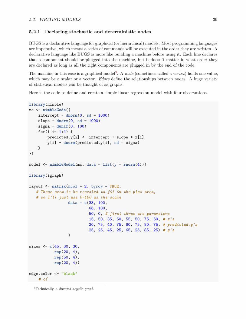
5.2.1 Declaring stochastic and deterministic nodes
BUGS is a declarative language for graphical (or hierarchical) models. Most programming languagesare imperative, which means a series of commands will be executed in the order they are written. Adeclarative language like BUGS is more like building a machine before using it. Each line declaresthat a component should be plugged into the machine, but it doesn’t matter in what order theyare declared as long as all the right components are plugged in by the end of the code.
The machine in this case is a graphical model3. A node (sometimes called a vertex) holds one value,which may be a scalar or a vector. Edges define the relationships between nodes. A huge varietyof statistical models can be thought of as graphs.
Here is the code to define and create a simple linear regression model with four observations.
library(nimble)mc <- nimbleCode({
intercept ~ dnorm(0, sd = 1000)slope ~ dnorm(0, sd = 1000)sigma ~ dunif(0, 100)for(i in 1:4) {
predicted.y[i] <- intercept + slope * x[i]y[i] ~ dnorm(predicted.y[i], sd = sigma)
}})
model <- nimbleModel(mc, data = list(y = rnorm(4)))
library(igraph)
layout <- matrix(ncol = 2, byrow = TRUE,# These seem to be rescaled to fit in the plot area,# so I'll just use 0-100 as the scale
data = c(33, 100,66, 100,50, 0, # first three are parameters15, 50, 35, 50, 55, 50, 75, 50, # x's20, 75, 40, 75, 60, 75, 80, 75, # predicted.y's25, 25, 45, 25, 65, 25, 85, 25) # y's
)
sizes <- c(45, 30, 30,rep(20, 4),rep(50, 4),rep(20, 4))
edge.color <- "black"# c(
3Technically, a directed acyclic graph

40 CHAPTER 5. WRITING MODELS IN NIMBLE’S DIALECT OF BUGS
# rep("green", 8),# rep("red", 4),# rep("blue", 4),# rep("purple", 4))
stoch.color <- "deepskyblue2"det.color <- "orchid3"rhs.color <- "gray73"fill.color <- c(
rep(stoch.color, 3),rep(rhs.color, 4),rep(det.color, 4),rep(stoch.color, 4)
)
plot(model$graph, vertex.shape = "crectangle",vertex.size = sizes,vertex.size2 = 20,layout = layout,vertex.label.cex = 3.0,vertex.color = fill.color,edge.width = 3,asp = 0.5,edge.color = edge.color)
intercept slope
sigma
x[1] x[2] x[3] x[4]
predicted.y[1] predicted.y[2] predicted.y[3] predicted.y[4]
y[1] y[2] y[3] y[4]
Figure 5.1: Graph of a linear regression model
The graph representing the model is shown in Figure 5.1. Each observation, y[i], is a node whoseedges say that it follows a normal distribution depending on a predicted value, predicted.y[i],
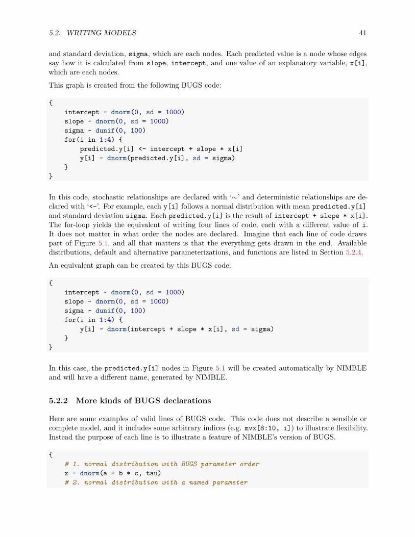
5.2. WRITING MODELS 41
and standard deviation, sigma, which are each nodes. Each predicted value is a node whose edgessay how it is calculated from slope, intercept, and one value of an explanatory variable, x[i],which are each nodes.This graph is created from the following BUGS code:
{intercept ~ dnorm(0, sd = 1000)slope ~ dnorm(0, sd = 1000)sigma ~ dunif(0, 100)for(i in 1:4) {
predicted.y[i] <- intercept + slope * x[i]y[i] ~ dnorm(predicted.y[i], sd = sigma)
}}
In this code, stochastic relationships are declared with ‘∼’ and deterministic relationships are de-clared with ‘<-’. For example, each y[i] follows a normal distribution with mean predicted.y[i]and standard deviation sigma. Each predicted.y[i] is the result of intercept + slope * x[i].The for-loop yields the equivalent of writing four lines of code, each with a different value of i.It does not matter in what order the nodes are declared. Imagine that each line of code drawspart of Figure 5.1, and all that matters is that the everything gets drawn in the end. Availabledistributions, default and alternative parameterizations, and functions are listed in Section 5.2.4.An equivalent graph can be created by this BUGS code:
{intercept ~ dnorm(0, sd = 1000)slope ~ dnorm(0, sd = 1000)sigma ~ dunif(0, 100)for(i in 1:4) {
y[i] ~ dnorm(intercept + slope * x[i], sd = sigma)}
}
In this case, the predicted.y[i] nodes in Figure 5.1 will be created automatically by NIMBLEand will have a different name, generated by NIMBLE.
5.2.2 More kinds of BUGS declarations
Here are some examples of valid lines of BUGS code. This code does not describe a sensible orcomplete model, and it includes some arbitrary indices (e.g. mvx[8:10, i]) to illustrate flexibility.Instead the purpose of each line is to illustrate a feature of NIMBLE’s version of BUGS.
{# 1. normal distribution with BUGS parameter orderx ~ dnorm(a + b * c, tau)# 2. normal distribution with a named parameter
42 CHAPTER 5. WRITING MODELS IN NIMBLE’S DIALECT OF BUGS
y ~ dnorm(a + b * c, sd = sigma)# 3. For-loop and nested indexingfor(i in 1:N) {
for(j in 1:M[i]) {z[i,j] ~ dexp(r[ blockID[i] ])
}}# 4. multivariate distribution with arbitrary indexingfor(i in 1:3)
mvx[8:10, i] ~ dmnorm(mvMean[3:5], cov = mvCov[1:3, 1:3, i])# 5. User-provided distributionw ~ dMyDistribution(hello = x, world = y)# 6. Simple deterministic noded1 <- a + b# 7. Vector deterministic node with matrix multiplicationd2[] <- A[ , ] %*% mvMean[1:5]# 8. Deterministic node with user-provided functiond3 <- foo(x, hooray = y)
}
When a variable appears only on the right-hand side, it can be provided via constants (in whichcase it can never be changed) or via data or inits, as discussed in Chapter 6.
Notes on the comment-numbered lines are:
1. x follows a normal distribution with mean a + b*c and precision tau (default BUGS secondparameter for dnorm).
2. y follows a normal distribution with the same mean as x but a named standard deviationparameter instead of a precision parameter (sd = 1/sqrt(precision)).
3. z[i, j] follows an exponential distribution with parameter r[ blockID[i] ]. This showshow for-loops can be used for indexing of variables containing multiple nodes. Variables thatdefine for-loop indices (N and M) must also be provided as constants.
4. The arbitrary block mvx[8:10, i] follows a multivariate normal distribution, with a namedcovariance matrix instead of BUGS’ default of a precision matrix. As in R, curly braces forfor-loop contents are only needed if there is more than one line.
5. w follows a user-defined distribution. See Chapter 12.6. d1 is a scalar deterministic node that, when calculated, will be set to a + b.7. d2 is a vector deterministic node using matrix multiplication in R’s syntax.8. d3 is a deterministic node using a user-provided function. See Chapter 12.
5.2.2.1 More about indexing
Examples of allowed indexing include:
• x[i] # a single index• x[i:j] # a range of indices
5.2. WRITING MODELS 43
• x[i:j,k:l] # multiple single indices or ranges for higher-dimensional arrays• x[i:j, ] # blank indices indicating the full range• x[3*i+7] # computed indices• x[(3*i):(5*i+1)] # computed lower and upper ends of an index range• x[k[i]+1] # a dynamic (and computed) index• x[k[j[i]]] # nested dynamic indexes• x[k[i], 1:3] # nested indexing of rows or columns
NIMBLE does not allow multivariate nodes to be used without square brackets, which is an incom-patibility with JAGS. Therefore a statement like xbar <- mean(x) in JAGS must be converted toxbar <- mean(x[]) (if x is a vector) or xbar <- mean(x[,]) (if x is a matrix) for NIMBLE4.Section 6.1.1.5 discusses how to provide NIMBLE with dimensions of x when needed.
Generally NIMBLE supports R-like linear algebra expressions and attempts to follow the samerules as R about dimensions (although in some cases this is not possible). For example, x[1:3]%*% y[1:3] converts x[1:3] into a row vector and thus computes the inner product, which isreturned as a 1 × 1 matrix (use inprod to get it as a scalar, which it typically easier). Like in R, ascalar index will result in dropping a dimension unless the argument drop=FALSE is provided. Forexample, mymatrix[i, 1:3] will be a vector of length 3, but mymatrix[i, 1:3, drop=FALSE]will be a 1 × 3 matrix. More about indexing and dimensions is discussed in Section 11.3.2.6.
5.2.3 Vectorized versus scalar declarations
Suppose you need nodes logY[i] that should be the log of the corresponding Y[i], say for i from1 to 10. Conventionally this would be created with a for loop:
{for(i in 1:10) {
logY[i] <- log(Y[i])}
}
Since NIMBLE supports R-like algebraic expressions, an alternative in NIMBLE’s dialect of BUGSis to use a vectorized declaration like this:
{logY[1:10] <- log(Y[1:10])
}
There is an important difference between the models that are created by the above two methods.The first creates 10 scalar nodes, logY[1] , . . . , logY[10]. The second creates one vector node,logY[1:10]. If each logY[i] is used separately by an algorithm, it may be more efficient compu-tationally if they are declared as scalars. If they are all used together, it will often make sense todeclare them as a vector.
4In nimbleFunctions, as explained in later chapters, square brackets with blank indices are not necessary formultivariate objects.

44 CHAPTER 5. WRITING MODELS IN NIMBLE’S DIALECT OF BUGS
5.2.4 Available distributions
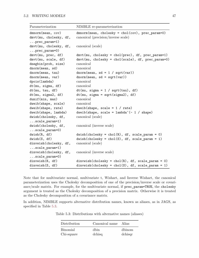
5.2.4.1 Distributions
NIMBLE supports most of the distributions allowed in BUGS and JAGS. Table 5.1 lists the distri-butions that are currently supported, with their default parameterizations, which match those ofBUGS5. NIMBLE also allows one to use alternative parameterizations for a variety of distributionsas described next. See Section 12.2 to learn how to write new distributions using nimbleFunctions.
Table 5.1: Distributions with their default order of parame-ters. The value of the random variable is denoted by x.
Name Usage Density Lower UpperBernoulli dbern(prob = p) px(1 − p)1−x 0 1
0 < p < 1Beta dbeta(shape1 = a, xa−1(1−x)b−1
β(a,b) 0 1shape2 = b), a > 0, b > 0
Binomial dbin(prob = p, size = n)(n
x
)px(1 − p)n−x 0 n
0 < p < 1, n ∈ N∗
CAR dcar_normal(adj, weights, see chapter 9 for details(intrinsic) num, tau, c, zero_meanCAR dcar_proper(mu, C, adj, see chapter 9 for details(proper) num, M, tau, gamma)Categorical dcat(prob = p) px∑
ipi
1 N
p ∈ (R+)N
Chi-square dchisq(df = k), k > 0 xk2 −1 exp(−x/2)
2k2 Γ( k
2 )0
Dirichlet ddirch(alpha = α) Γ(∑
j αj)∏
j
xαj −1j
Γ(αj) 0αj ≥ 0
Exponential dexp(rate = λ), λ > 0 λ exp(−λx) 0Flat dflat() ∝ 1 (improper)Gamma dgamma(shape = r, rate = λ) λrxr−1 exp(−λx)
Γ(r) 0λ > 0, r > 0
Half flat dhalfflat() ∝ 1 (improper) 0Inverse dinvgamma(shape = r, scale = λ) λrx−(r+1) exp(−λ/x)
Γ(r) 0gamma λ > 0, r > 0Logistic dlogis(location = µ, τ exp{(x−µ)τ}
[1+exp{(x−µ)τ}]2
rate = τ),τ > 0Log-normal dlnorm(meanlog = µ,
(τ
2π
) 12 x−1 exp
{−τ(log(x) − µ)2/2
}0
taulog = τ), τ > 0
Multinomial dmulti(prob = p, size = n) n!∏
j
pxjj
xj !
5Note that the same distributions are available for writing nimbleFunctions, but in that case the default param-eterizations and function names match R’s when possible. Please see Section 11.2.4 for how to use distributions innimbleFunctions.

5.2. WRITING MODELS 45
Name Usage Density Lower Upper∑j xj = n
Multivariate dmnorm(mean = µ, prec = Λ) (2π)− d2 |Λ|
12 exp{− (x−µ)T Λ(x−µ)
2 }normal Λ positive definiteMultivariate dmvt(mu = µ, prec = Λ) Γ( ν+d
2 )Γ( ν
2 )(νπ)d/2 |Λ|1/2(1 + (x−µ)T Λ(x−µ)ν )− ν+d
2
Student t df = ν), Λ positive def.Negative dnegbin(prob = p, size = r)
(x+r−1x
)pr(1 − p)x 0
binomial 0 < p ≤ 1, r ≥ 0Normal dnorm(mean = µ, tau = τ)
(τ
2π
) 12 exp{−τ(x − µ)2/2}
τ > 0Poisson dpois(lambda = λ) exp(−λ)λx
x! 0λ > 0
Student t dt(mu = µ, tau = τ, df = k) Γ( k+12 )
Γ( k2 )
(τ
kπ
) 12
{1 + τ(x−µ)2
k
}− (k+1)2
τ > 0, k > 0Uniform dunif(min = a, max = b) 1
b−a a b
a < bWeibull dweib(shape = v, lambda = λ) vλxv−1 exp(−λxv) 0
v > 0, λ > 0Wishart dwish(R = R, df = k) |x|(k−p−1)/2|R|k/2 exp{−tr(Rx)/2}
2pk/2πp(p−1)/4∏p
i=1 Γ((k+1−i)/2)R p × p pos. def., k ≥ p
Inverse dinvwish(S = S, df = k) |x|−(k+p+1)/2|S|k/2 exp{−tr(Sx−1)/2}2pk/2πp(p−1)/4
∏p
i=1 Γ((k+1−i)/2)Wishart S p × p pos. def., k ≥ p
5.2.4.1.1 Improper distributions
Note that dcar_normal, dflat and dhalfflat specify improper prior distributions and shouldonly be used when the posterior distribution of the model is known to be proper. Also for thesedistributions, the density function returns the unnormalized density and the simulation functionreturns NaN so these distributions are not appropriate for algorithms that need to simulate fromthe prior or require proper (normalized) densities.
5.2.4.2 Alternative parameterizations for distributions
NIMBLE allows one to specify distributions in model code using a variety of parameterizations,including the BUGS parameterizations. Available parameterizations are listed in Table 5.2. Tounderstand how NIMBLE handles alternative parameterizations, it is useful to distinguish threecases, using the gamma distribution as an example:
1. A canonical parameterization is used directly for computations6. For gamma, this is (shape,scale).
6Usually this is the parameterization in the Rmath header of R’s C implementation of distributions.

46 CHAPTER 5. WRITING MODELS IN NIMBLE’S DIALECT OF BUGS
2. The BUGS parameterization is the one defined in the original BUGS language. In general thisis the parameterization for which conjugate MCMC samplers can be executed most efficiently.For dgamma, this is (shape, rate).
3. An alternative parameterization is one that must be converted into the canonical parameter-ization. For dgamma, NIMBLE provides both (shape, rate) and (mean, sd) parameterizationand creates nodes to calculate (shape, scale) from either (shape, rate) or (mean, sd). In thecase of dgamma, the BUGS parameterization is also an alternative parameterization.
Since NIMBLE provides compatibility with existing BUGS and JAGS code, the order of parame-ters places the BUGS parameterization first. For example, the order of parameters for dgamma isdgamma(shape, rate, scale, mean, sd). Like R, if parameter names are not given, they aretaken in order, so that (shape, rate) is the default. This happens to match R’s order of parameters,but it need not. If names are given, they can be given in any order. NIMBLE knows that rate isan alternative to scale and that (mean, sd) are an alternative to (shape, scale or rate).
Table 5.2: Distribution parameterizations allowed in NIM-BLE. The first column indicates the supported parameteriza-tions for distributions given in Table 5.1. The second columnindicates the relationship to the canonical parameterizationused in NIMBLE.
Parameterization NIMBLE re-parameterizationdbern(prob) dbin(size = 1, prob)dbeta(shape1, shape2) canonicaldbeta(mean, sd) dbeta(shape1 = meanˆ2 * (1-mean) / sdˆ2 - mean,
shape2 = mean * (1 - mean)ˆ2 / sdˆ2 + mean - 1)dbin(prob, size) canonicaldcat(prob) canonicaldchisq(df) canonicalddirch(alpha) canonicaldexp(rate) canonicaldexp(scale) dexp(rate = 1/scale)dgamma(shape, scale) canonicaldgamma(shape, rate) dgamma(shape, scale = 1 / rate)dgamma(mean, sd) dgamma(shape = meanˆ2/sdˆ2, scale = sdˆ2/mean)dinvgamma(shape, rate) canonicaldinvgamma(shape, scale) dgamma(shape, rate = 1 / scale)dlogis(location, scale) canonicaldlogis(location, rate) dlogis(location, scale = 1 / ratedlnorm(meanlog, sdlog) canonicaldlnorm(meanlog, taulog) dlnorm(meanlog, sdlog = 1 / sqrt(taulog)dlnorm(meanlog, varlog) dlnorm(meanlog, sdlog = sqrt(varlog)dmulti(prob, size) canonicaldmnorm(mean, cholesky, canonical (precision)...prec_param=1)dmnorm(mean, cholesky, canonical (covariance)...prec_param=0)dmnorm(mean, prec) dmnorm(mean, cholesky = chol(prec), prec_param=1)
5.2. WRITING MODELS 47
Parameterization NIMBLE re-parameterizationdmnorm(mean, cov) dmnorm(mean, cholesky = chol(cov), prec_param=0)dmvt(mu, cholesky, df, canonical (precision/inverse scale)...prec_param=1)dmvt(mu, cholesky, df, canonical (scale)...prec_param=0)dmvt(mu, prec, df) dmvt(mu, cholesky = chol(prec), df, prec_param=1)dmvt(mu, scale, df) dmvt(mu, cholesky = chol(scale), df, prec_param=0)dnegbin(prob, size) canonicaldnorm(mean, sd) canonicaldnorm(mean, tau) dnorm(mean, sd = 1 / sqrt(var))dnorm(mean, var) dnorm(mean, sd = sqrt(var))dpois(lambda) canonicaldt(mu, sigma, df) canonicaldt(mu, tau, df) dt(mu, sigma = 1 / sqrt(tau), df)dt(mu, sigma2, df) dt(mu, sigma = sqrt(sigma2), df)dunif(min, max) canonicaldweib(shape, scale) canonicaldweib(shape, rate) dweib(shape, scale = 1 / rate)dweib(shape, lambda) dweib(shape, scale = lambdaˆ(- 1 / shape)dwish(cholesky, df, canonical (scale)...scale_param=1)dwish(cholesky, df, canonical (inverse scale)...scale_param=0)dwish(R, df) dwish(cholesky = chol(R), df, scale_param = 0)dwish(S, df) dwish(cholesky = chol(S), df, scale_param = 1)dinvwish(cholesky, df, canonical (scale)...scale_param=1)dinvwish(cholesky, df, canonical (inverse scale)...scale_param=0)dinvwish(R, df) dinvwish(cholesky = chol(R), df, scale_param = 0)dinvwish(S, df) dinvwish(cholesky = chol(S), df, scale_param = 1)
Note that for multivariate normal, multivariate t, Wishart, and Inverse Wishart, the canonicalparameterization uses the Cholesky decomposition of one of the precision/inverse scale or covari-ance/scale matrix. For example, for the multivariate normal, if prec_param=TRUE, the choleskyargument is treated as the Cholesky decomposition of a precision matrix. Otherwise it is treatedas the Cholesky decomposition of a covariance matrix.
In addition, NIMBLE supports alternative distribution names, known as aliases, as in JAGS, asspecified in Table 5.3.
Table 5.3: Distributions with alternative names (aliases)
Distribution Canonical name AliasBinomial dbin dbinomChi-square dchisq dchisqr

48 CHAPTER 5. WRITING MODELS IN NIMBLE’S DIALECT OF BUGS
Distribution Canonical name AliasDirichlet ddirch ddirichMultinomial dmulti dmultinomNegative binomial dnegbin dnbinomWeibull dweib dweibullWishart dwish dwishart
We plan to, but do not currently, include the following distributions as part of core NIMBLE: doubleexponential (Laplace), beta-binomial, Dirichlet-multinomial, F, Pareto, or forms of the multivariatet other than the standard one provided.
5.2.5 Available BUGS language functions
Tables 11.2-11.3 show the available operators and functions. Support for more general R expressionsis covered in Chapter 11 about programming with nimbleFunctions.
For the most part NIMBLE supports the functions used in BUGS and JAGS, with exceptionsindicated in the table. Additional functions provided by NIMBLE are also listed. Note that weprovide distribution functions for use in calculations, namely the ‘p’, ‘q’, and ‘d’ functions. SeeSection 11.2.4 for details on the syntax for using distribution functions as functions in deterministiccalculations, as only some parameterizations are allowed and the names of some distributions differfrom those used to define stochastic nodes in a model.
Table 5.4: Functions operating on scalars, many of whichcan operate on each element (component-wise) of vectors andmatrices. Status column indicates if the function is currentlyprovided in NIMBLE. Vector input column indicates if thefunction can take a vector as an argument (i.e., if the functionis vectorized).
Usage Description Comments Status Vector inputx | y, x & y logical OR (|) and AND(&) yes yes!x logical not yes yesx > y, x >= y greater than (and or equal to) yes yesx < y, x <= y less than (and or equal to) yes yesx != y, x == y (not) equals yes yesx + y, x - y, x * y component-wise operators mix of scalar and vector yes yesx / y component-wise division vector x and scalar y yes yesxˆy, pow(x, y) power xy; vector x,scalar y yes yesx %% y modulo (remainder) yes nomin(x1, x2), min. (max.) of two scalars yes See pmin,max(x1, x2) pmaxexp(x) exponential yes yeslog(x) natural logarithm yes yessqrt(x) square root yes yesabs(x) absolute value yes yes
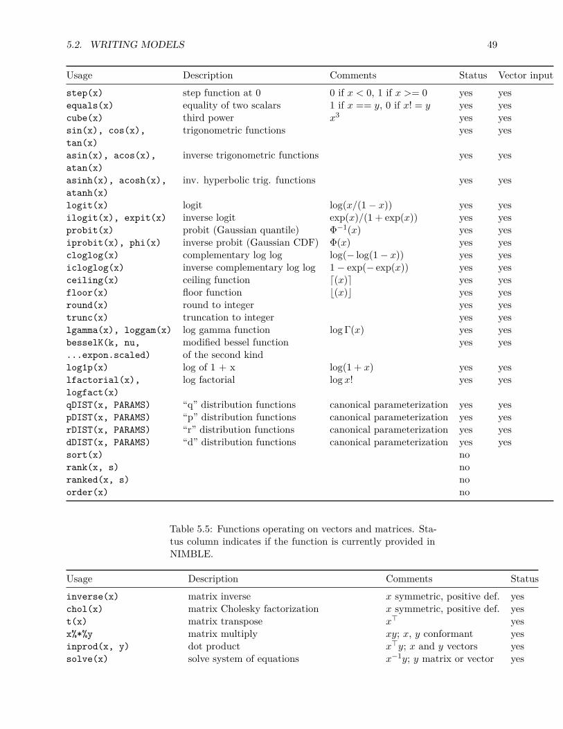
5.2. WRITING MODELS 49
Usage Description Comments Status Vector inputstep(x) step function at 0 0 if x < 0, 1 if x >= 0 yes yesequals(x) equality of two scalars 1 if x == y, 0 if x! = y yes yescube(x) third power x3 yes yessin(x), cos(x), trigonometric functions yes yestan(x)asin(x), acos(x), inverse trigonometric functions yes yesatan(x)asinh(x), acosh(x), inv. hyperbolic trig. functions yes yesatanh(x)logit(x) logit log(x/(1 − x)) yes yesilogit(x), expit(x) inverse logit exp(x)/(1 + exp(x)) yes yesprobit(x) probit (Gaussian quantile) Φ−1(x) yes yesiprobit(x), phi(x) inverse probit (Gaussian CDF) Φ(x) yes yescloglog(x) complementary log log log(− log(1 − x)) yes yesicloglog(x) inverse complementary log log 1 − exp(− exp(x)) yes yesceiling(x) ceiling function ⌈(x)⌉ yes yesfloor(x) floor function ⌊(x)⌋ yes yesround(x) round to integer yes yestrunc(x) truncation to integer yes yeslgamma(x), loggam(x) log gamma function log Γ(x) yes yesbesselK(k, nu, modified bessel function yes yes...expon.scaled) of the second kindlog1p(x) log of 1 + x log(1 + x) yes yeslfactorial(x), log factorial log x! yes yeslogfact(x)qDIST(x, PARAMS) “q” distribution functions canonical parameterization yes yespDIST(x, PARAMS) “p” distribution functions canonical parameterization yes yesrDIST(x, PARAMS) “r” distribution functions canonical parameterization yes yesdDIST(x, PARAMS) “d” distribution functions canonical parameterization yes yessort(x) norank(x, s) noranked(x, s) noorder(x) no
Table 5.5: Functions operating on vectors and matrices. Sta-tus column indicates if the function is currently provided inNIMBLE.
Usage Description Comments Statusinverse(x) matrix inverse x symmetric, positive def. yeschol(x) matrix Cholesky factorization x symmetric, positive def. yest(x) matrix transpose x⊤ yesx%*%y matrix multiply xy; x, y conformant yesinprod(x, y) dot product x⊤y; x and y vectors yessolve(x) solve system of equations x−1y; y matrix or vector yes

50 CHAPTER 5. WRITING MODELS IN NIMBLE’S DIALECT OF BUGS
Usage Description Comments Statusforwardsolve(x, y) solve lower-triangular system of equations x−1y; x lower-triangular yesbacksolve(x, y) solve upper-triangular system of equations x−1y; x upper-triangular yeslogdet(x) log matrix determinant log |x| yesasRow(x) convert vector to 1-row matrix sometimes automatic yesasCol(x) convert vector to 1-column matrix sometimes automatic yessum(x) sum of elements of x yesmean(x) mean of elements of x yessd(x) standard deviation of elements of x yesprod(x) product of elements of x yesmin(x), max(x) min. (max.) of elements of x yespmin(x, y), pmax(x,y) vector of mins (maxs) of elements of yes
x and yinterp.lin(x, v1, v2) linear interpolation noeigen(x)$values matrix eigenvalues x symmetric yeseigen(x)$vectors matrix eigenvectors x symmetric yessvd(x)$d matrix singular values yessvd(x)$u matrix left singular vectors yessvd(x)$v matrix right singular vectors yes
See Section 12.1 to learn how to use nimbleFunctions to write new functions for use in BUGS code.
5.2.6 Available link functions
NIMBLE allows the link functions listed in Table 5.6.
Table 5.6: Link functions.
Link function Description Range Inversecloglog(y) <- x Complementary log log 0 < y < 1 y <- icloglog(x)log(y) <- x Log 0 < y y <- exp(x)logit(y) <- x Logit 0 < y < 1 y <- expit(x)probit(y) <- x Probit 0 < y < 1 y <- iprobit(x)
Link functions are specified as functions applied to a node on the left hand side of a BUGS expression.To handle link functions in deterministic declarations, NIMBLE converts the declaration into anequivalent inverse declaration. For example, log(y) <- x is converted into y <- exp(x). In otherwords, the link function is just a simple variant for conceptual clarity.
To handle link functions in a stochastic declaration, NIMBLE does some processing that inserts anadditional node into the model. For example, the declaration logit(p[i]) ~ dnorm(mu[i],1), isequivalent to the following two declarations:
• logit_p[i] ~ dnorm(mu[i], 1),• p[i] <- expit(logit_p[i])

5.2. WRITING MODELS 51
where expit is the inverse of logit.
Note that NIMBLE does not provide an automatic way of initializing the additional node(logit_p[i] in this case), which is a parent node of the explicit node (p[i]), without explicitlyreferring to the additional node by the name that NIMBLE generates.
5.2.7 Truncation, censoring, and constraints
NIMBLE provides three ways to declare boundaries on the value of a variable, each for differentsituations. We introduce these and comment on their relationships to related features of JAGS andBUGS. The three methods are:
5.2.7.1 Truncation
Either of the following forms,
x ~ dnorm(0, sd = 10) T(0, a)x ~ T(dnorm(0, sd = 10), 0, a)
declares that x follows a normal distribution between 0 and a (inclusive of 0 and a). Either boundarymay be omitted or may be another node, such as a in this example. The first form is compatiblewith JAGS, but in NIMBLE it can only be used when reading code from a text file. When writingmodel code in R, the second version must be used.
Truncation means the possible values of x are limited a priori, hence the probability density of xmust be normalized7. In this example it would be the normal probability density divided by itsintegral from 0 to a. Like JAGS, NIMBLE also provides I as a synonym for T to accommodateolder BUGS code, but T is preferred because it disambiguates multiple usages of I in BUGS.
5.2.7.2 Censoring
Censoring refers to the situation where one datum gives the lower or upper bound on an unobservedrandom variable. This is common in survival analysis, when for an individual still surviving at theend of a study, the age of death is not known and hence is ‘censored’ (right-censoring). NIMBLEadopts JAGS syntax for censoring, as follows:
censored[i] ~ dinterval(t[i], c[i])t[i] ~ dweib(r, mu[i])
In the case of right-censoring, censored[i] should be given as data with a value of 1 if t[i]is right-censored (t[i] > c[i]) and 0 if it is observed. The data vector for t should have NA(indicating missing data) for any censored t[i] entries. (As a result, these nodes will be sampledin an MCMC.) The data vector for c should give the censoring times corresponding to censored
7NIMBLE uses the CDF and inverse CDF (quantile) functions of a distribution to do this; in some cases if oneuses truncation to include only the extreme tail of a distribution, numerical difficulties can arise.

52 CHAPTER 5. WRITING MODELS IN NIMBLE’S DIALECT OF BUGS
entries and a value above the observed times for uncensored entries (e.g., Inf). Left-censoredobservations would be specified by setting censored[i] to 0 and t[i] to NA.The dinterval is not really a distribution but rather a trick: in the above example whencensored[i] = 1 it gives a ‘probability’ of 1 if t[i] > c[i] and 0 otherwise. This meansthat t[i] <= c[i] is treated as impossible. More generally than simple right- or left-censoring,censored[i] ~ dinterval(t[i], c[i, ]) is defined such that for a vector of increasingcutpoints, c[i, ], t[i] is enforced to fall within the censored[i]-th cutpoint interval. This isdone by setting data censored[i] as follows:censored[i] = 0 if t[i] <= c[i, 1]
censored[i] = m if c[i, m] < t[i] <= c[i, m+1] for 1 ≤ m ≤ M
censored[i] = M if c[i, M] < t[i]
(The i index is provided only for consistency with the previous example.) The most common usesof dinterval will be for left- and right-censored data, in which case c[i,] will be a single value(and typically given as simply c[i]), and for interval-censored data, in which case c[i,] will be avector of two values.
Nodes following a dinterval distribution should normally be set as data with known values. Oth-erwise, the node may be simulated during initialization in some algorithms (e.g., MCMC) andthereby establish a permanent, perhaps unintended, constraint.Censoring differs from truncation because censoring an observation involves bounds on a randomvariable that could have taken any value, while in truncation we know a priori that a datum couldnot have occurred outside the truncation range.
5.2.7.3 Constraints and ordering
NIMBLE provides a more general way to enforce constraints using dconstraint(cond). For ex-ample, we could specify that the sum of mu1 and mu2 must be positive like this:
mu1 ~ dnorm(0, 1)mu2 ~ dnorm(0, 1)constraint_data ~ dconstraint( mu1 + mu2 > 0 )
with constraint_data set (as data) to 1. This is equivalent to a half-normal distribution on thehalf-plane µ1 + µ2 > 0. Nodes following dconstraint should be provided as data for the samereason of avoiding unintended initialization described above for dinterval.Formally, dconstraint(cond) is a probability distribution on {0, 1} such that P (1) = 1 if cond isTRUE and P (0) = 1 if cond is FALSE.Of course, in many cases, parameterizing the model so that the constraints are automaticallyrespected may be a better strategy than using dconstraint. One should be cautious about con-straints that would make it hard for an MCMC or optimization to move through the parameterspace (such as equality constraints that involve two or more parameters). For such restrictive con-straints, general purpose algorithms that are not tailored to the constraints may fail or be inefficient.If constraints are used, it will generally be wise to ensure the model is initialized with values thatsatisfy them.
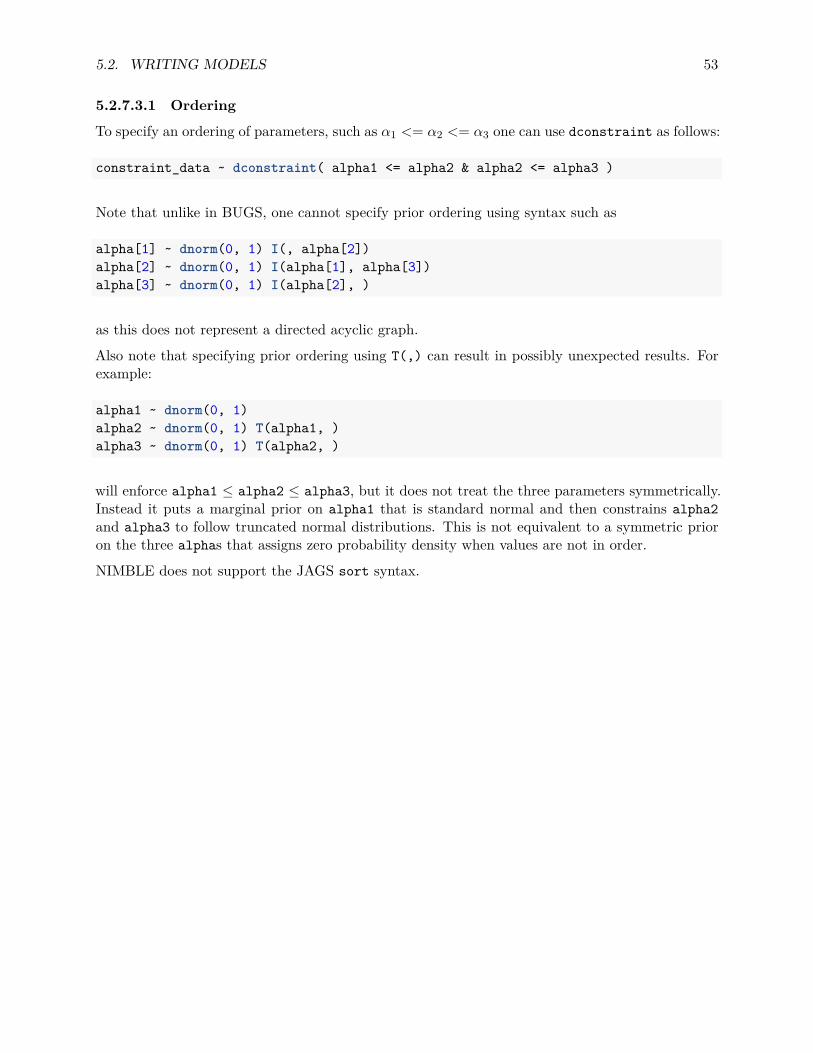
5.2. WRITING MODELS 53
5.2.7.3.1 Ordering
To specify an ordering of parameters, such as α1 <= α2 <= α3 one can use dconstraint as follows:
constraint_data ~ dconstraint( alpha1 <= alpha2 & alpha2 <= alpha3 )
Note that unlike in BUGS, one cannot specify prior ordering using syntax such as
alpha[1] ~ dnorm(0, 1) I(, alpha[2])alpha[2] ~ dnorm(0, 1) I(alpha[1], alpha[3])alpha[3] ~ dnorm(0, 1) I(alpha[2], )
as this does not represent a directed acyclic graph.
Also note that specifying prior ordering using T(,) can result in possibly unexpected results. Forexample:
alpha1 ~ dnorm(0, 1)alpha2 ~ dnorm(0, 1) T(alpha1, )alpha3 ~ dnorm(0, 1) T(alpha2, )
will enforce alpha1 ≤ alpha2 ≤ alpha3, but it does not treat the three parameters symmetrically.Instead it puts a marginal prior on alpha1 that is standard normal and then constrains alpha2and alpha3 to follow truncated normal distributions. This is not equivalent to a symmetric prioron the three alphas that assigns zero probability density when values are not in order.
NIMBLE does not support the JAGS sort syntax.

54 CHAPTER 5. WRITING MODELS IN NIMBLE’S DIALECT OF BUGS

Chapter 6
Building and using models
This chapter explains how to build and manipulate model objects starting from BUGS code.
6.1 Creating model objects
NIMBLE provides two functions for creating model objects: nimbleModel and readBUGSmodel. Thefirst, nimbleModel, is more general and was illustrated in Chapter 2. The second, readBUGSmodelprovides compatibility with BUGS file formats for models, variables, data, and initial values forMCMC.
In addition one can create new model objects from existing model objects.
6.1.1 Using nimbleModel to create a model
nimbleModel processes BUGS code to determine all the nodes, variables, and their relationshipsin a model. Any constants must be provided at this step. Data and initial values can optionallybe provided. BUGS code passed to nimbleModel must go through nimbleCode.
We look again at the pump example from the introduction:
pumpCode <- nimbleCode({for (i in 1:N){
theta[i] ~ dgamma(alpha,beta);lambda[i] <- theta[i]*t[i];x[i] ~ dpois(lambda[i])
}alpha ~ dexp(1.0);beta ~ dgamma(0.1,1.0);
})
pumpConsts <- list(N = 10,t = c(94.3, 15.7, 62.9, 126, 5.24,31.4, 1.05, 1.05, 2.1, 10.5))
55

56 CHAPTER 6. BUILDING AND USING MODELS
pumpData <- list(x = c(5, 1, 5, 14, 3, 19, 1, 1, 4, 22))
pumpInits <- list(alpha = 1, beta = 1,theta = rep(0.1, pumpConsts$N))
pump <- nimbleModel(code = pumpCode, name = "pump", constants = pumpConsts,data = pumpData, inits = pumpInits)
6.1.1.1 Data and constants
NIMBLE makes a distinction between data and constants:
• Constants can never be changed and must be provided when a model is defined. For example,a vector of known index values, such as for block indices, helps define the model graph itselfand must be provided as constants. Variables used in the index ranges of for-loops must alsobe provided as constants.
• Data is a label for the role a node plays in the model. Nodes marked as data will by defaultbe protected from any functions that would simulate over their values (see simulate inChapter 13), but it is possible to over-ride that default or to change their values by directassignment. This allows an algorithm to be applied to many data sets in the same modelwithout re-creating the model each time. It also allows simulation of data in a model.
WinBUGS, OpenBUGS and JAGS do not allow data values to be changed or different nodes to belabeled as data without starting from the beginning again. Hence they do not distinguish betweenconstants and data.
For compatibility with BUGS and JAGS, NIMBLE allows both to be provided in the constantsargument to nimbleModel, in which case NIMBLE handles values for stochastic nodes as data andeverything else as constants.
Values for nodes that appear only on the right-hand side of BUGS declarations (e.g., covari-ates/predictors) can be provided as constants or as data or initial values. There is no real differencebetween providing as data or initial values and the values can be added after building a model viasetInits or setData.
6.1.1.2 Providing data and initial values to an existing model
Whereas constants must be provided during the call to nimbleModel, data and initial values can beprovided later via the model member functions setData and setInits. For example, if pumpDatais a named list of data values (as above), then pump$setData(pumpData) sets the named variablesto the values in the list.
setData does two things: it sets the values of the data nodes, and it flags those nodes as containingdata. nimbleFunction programmers can then use that information to control whether an algorithmshould over-write data or not. For example, NIMBLE’s simulate functions by default do notoverwrite data values but can be told to do so. Values of data variables can be replaced, and the

6.1. CREATING MODEL OBJECTS 57
indication of which nodes should be treated as data can be reset by using the resetData method,e.g. pump$resetData().
6.1.1.3 Missing data values
Sometimes one needs a model variable to have a mix of data and non-data, often due to missingdata values. In NIMBLE, when data values are provided, any nodes with NA values will not belabeled as data. A node following a multivariate distribution must be either entirely observed orentirely missing.
Here’s an example of running an MCMC on the pump model, with two of the observations takento be missing. Some of the steps in this example are documented more below. NIMBLE’s defaultMCMC configuration will treat the missing values as unknowns to be sampled, as can be seen inthe MCMC output here.
pumpMiss <- pump$newModel()pumpMiss$resetData()pumpDataNew <- pumpDatapumpDataNew$x[c(1, 3)] <- NApumpMiss$setData(pumpDataNew)
pumpMissConf <- configureMCMC(pumpMiss)pumpMissConf$addMonitors('x', 'alpha', 'beta', 'theta')
## thin = 1: alpha, beta, x, theta
pumpMissMCMC <- buildMCMC(pumpMissConf)Cobj <- compileNimble(pumpMiss, pumpMissMCMC)
niter <- 10set.seed(0)Cobj$pumpMissMCMC$run(niter)
## NULL
samples <- as.matrix(Cobj$pumpMissMCMC$mvSamples)
samples[1:5, 13:17]
## x[1] x[2] x[3] x[4] x[5]## [1,] 17 1 2 14 3## [2,] 11 1 4 14 3## [3,] 14 1 9 14 3## [4,] 11 1 24 14 3## [5,] 9 1 29 14 3

58 CHAPTER 6. BUILDING AND USING MODELS
Missing values may also occur in explanatory/predictor variables. Values for such variables shouldbe passed in via the data argument to nimbleModel, with NA for the missing values. In somecontexts, one would want to specify distributions for such explanatory variables, for example sothat an MCMC would impute the missing values.
6.1.1.4 Defining alternative models with the same code
Avoiding code duplication is a basic principle of good programming. In NIMBLE, one can usedefinition-time if-then-else statements to create different models from the same code. As a simpleexample, say we have a linear regression model and want to consider including or omitting x[2] asan explanatory variable:
regressionCode <- nimbleCode({intercept ~ dnorm(0, sd = 1000)slope1 ~ dnorm(0, sd = 1000)if(includeX2) {
slope2 ~ dnorm(0, sd = 1000)for(i in 1:N)
predictedY[i] <- intercept + slope1 * x1[i] + slope2 * x2[i]} else {
for(i in 1:N) predictedY[i] <- intercept + slope1 * x1[i]}sigmaY ~ dunif(0, 100)for(i in 1:N) Y[i] ~ dnorm(predictedY[i], sigmaY)
})
includeX2 <- FALSEmodelWithoutX2 <- nimbleModel(regressionCode, constants = list(N = 30),
check=FALSE)modelWithoutX2$getVarNames()
## [1] "intercept" "slope1"## [3] "predictedY" "sigmaY"## [5] "lifted_d1_over_sqrt_oPsigmaY_cP" "Y"## [7] "x1"
includeX2 <- TRUEmodelWithX2 <- nimbleModel(regressionCode, constants = list(N = 30),
check = FALSE)modelWithX2$getVarNames()
## [1] "intercept" "slope1"## [3] "slope2" "predictedY"## [5] "sigmaY" "lifted_d1_over_sqrt_oPsigmaY_cP"## [7] "Y" "x1"## [9] "x2"

6.1. CREATING MODEL OBJECTS 59
Whereas the constants are a property of the model definition – since they may help determine themodel structure itself – data nodes can be different in different copies of the model generated fromthe same model definition. The setData and setInits described above can be used for each copyof the model.
6.1.1.5 Providing dimensions via nimbleModel
nimbleModel can usually determine the dimensions of every variable from the declarations in theBUGS code. However, it is possible to use a multivariate object only with empty indices (e.g. x[,]),in which case the dimensions must be provided as an argument to nimbleModel.
Here’s an example with multivariate nodes. The first provides indices, so no dimensions argumentis needed, while the second omits the indices and provides a dimensions argument instead.
code <- nimbleCode({y[1:K] ~ dmulti(p[1:K], n)p[1:K] ~ ddirch(alpha[1:K])log(alpha[1:K]) ~ dmnorm(alpha0[1:K], R[1:K, 1:K])
})
K <- 5model <- nimbleModel(code, constants = list(n = 3, K = K,
alpha0 = rep(0, K), R = diag(K)),check = FALSE)
codeAlt <- nimbleCode({y[] ~ dmulti(p[], n)p[] ~ ddirch(alpha[])log(alpha[]) ~ dmnorm(alpha0[], R[ , ])
})
model <- nimbleModel(codeAlt, constants = list(n = 3, K = K, alpha0 = rep(0, K),R = diag(K)),
dimensions = list(y = K, p = K, alpha = K),check = FALSE)
In that example, since alpha0 and R are provided as constants, we don’t need to specify theirdimensions.
6.1.2 Creating a model from standard BUGS and JAGS input files
Users with BUGS and JAGS experience may have files set up in standard formats for use inBUGS and JAGS. readBUGSmodel can read in the model, data/constant values and initial valuesin those formats. It can also take information directly from R objects somewhat more flexibly thannimbleModel, specifically allowing inputs set up similarly to those for BUGS and JAGS. In eithercase, after processing the inputs, it calls nimbleModel. Note that unlike BUGS and JAGS, only a
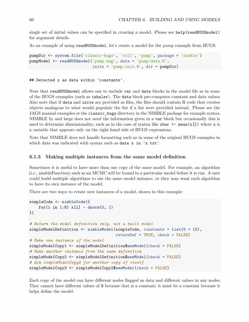
60 CHAPTER 6. BUILDING AND USING MODELS
single set of initial values can be specified in creating a model. Please see help(readBUGSmodel)for argument details.As an example of using readBUGSmodel, let’s create a model for the pump example from BUGS.
pumpDir <- system.file('classic-bugs', 'vol1', 'pump', package = 'nimble')pumpModel <- readBUGSmodel('pump.bug', data = 'pump-data.R',
inits = 'pump-init.R', dir = pumpDir)
## Detected x as data within 'constants'.
Note that readBUGSmodel allows one to include var and data blocks in the model file as in someof the BUGS examples (such as inhaler). The data block pre-computes constant and data values.Also note that if data and inits are provided as files, the files should contain R code that createsobjects analogous to what would populate the list if a list were provided instead. Please see theJAGS manual examples or the classic_bugs directory in the NIMBLE package for example syntax.NIMBLE by and large does not need the information given in a var block but occasionally this isused to determine dimensionality, such as in the case of syntax like xbar <- mean(x[]) where x isa variable that appears only on the right-hand side of BUGS expressions.Note that NIMBLE does not handle formatting such as in some of the original BUGS examples inwhich data was indicated with syntax such as data x in 'x.txt'.
6.1.3 Making multiple instances from the same model definition
Sometimes it is useful to have more than one copy of the same model. For example, an algorithm(i.e., nimbleFunction) such as an MCMC will be bound to a particular model before it is run. A usercould build multiple algorithms to use the same model instance, or they may want each algorithmto have its own instance of the model.There are two ways to create new instances of a model, shown in this example:
simpleCode <- nimbleCode({for(i in 1:N) x[i] ~ dnorm(0, 1)
})
# Return the model definition only, not a built modelsimpleModelDefinition <- nimbleModel(simpleCode, constants = list(N = 10),
returnDef = TRUE, check = FALSE)# Make one instance of the modelsimpleModelCopy1 <- simpleModelDefinition$newModel(check = FALSE)# Make another instance from the same definitionsimpleModelCopy2 <- simpleModelDefinition$newModel(check = FALSE)# Ask simpleModelCopy2 for another copy of itselfsimpleModelCopy3 <- simpleModelCopy2$newModel(check = FALSE)
Each copy of the model can have different nodes flagged as data and different values in any nodes.They cannot have different values of N because that is a constant; it must be a constant because ithelps define the model.
6.2. NIMBLE MODELS ARE OBJECTS YOU CAN QUERY AND MANIPULATE 61
6.2 NIMBLE models are objects you can query and manipulate
NIMBLE models are objects that can be modified and manipulated from R. In this section weintroduce some basic ways to use a model object. Chapter 13 covers more topics for writingalgorithms that use models.
6.2.1 What are variables and nodes?
This section discusses some basic concepts and terminology to be able to speak about NIMBLEmodels clearly.
Suppose we have created a model from the following BUGS code.
mc <- nimbleCode({a ~ dnorm(0, 0.001)for(i in 1:5) {
y[i] ~ dnorm(a, sd = 0.1)for(j in 1:3)
z[i,j] ~ dnorm(y[i], tau)}tau ~ dunif(0, 20)y.squared[1:5] <- y[1:5]^2
})
model <- nimbleModel(mc, data = list(z = matrix(rnorm(15), nrow = 5)))
In NIMBLE terminology:
• The variables of this model are a, y, z, and y.squared.• The nodes of this model are a, y[1] , . . . , y[5], z[1,1] , . . . , z[5, 3], and y.squared[1:5].
In graph terminology, nodes are vertices in the model graph.• The node functions of this model are a ~ dnorm(0, 0.001), y[i] ~ dnorm(a, 0.1),
z[i,j] ~ dnorm(y[i], sd = 0.1), and y.squared[1:5] <- y[1:5]ˆ2. Each node’scalculations are handled by a node function. Sometimes the distinction between nodes andnode functions is important, but when it is not important we may refer to both simply asnodes.
• The scalar elements of this model include all the scalar nodes as well as the scalar elementsy.squared[1] , . . . , y.squared[5] of the multivariate node y.squared[1:5].
6.2.2 Determining the nodes and variables in a model
One can determine the variables in a model using getVarNames and the nodes in a model usinggetNodeNames. Optional arguments to getNodeNames allow you to select only certain types ofnodes, as discussed in Section 13.1.1 and in the R help for getNodeNames.

62 CHAPTER 6. BUILDING AND USING MODELS
model$getVarNames()
## [1] "a" "y"## [3] "lifted_d1_over_sqrt_oPtau_cP" "z"## [5] "tau" "y.squared"
model$getNodeNames()
## [1] "a" "tau"## [3] "y[1]" "y[2]"## [5] "y[3]" "y[4]"## [7] "y[5]" "lifted_d1_over_sqrt_oPtau_cP"## [9] "y.squared[1:5]" "z[1, 1]"## [11] "z[1, 2]" "z[1, 3]"## [13] "z[2, 1]" "z[2, 2]"## [15] "z[2, 3]" "z[3, 1]"## [17] "z[3, 2]" "z[3, 3]"## [19] "z[4, 1]" "z[4, 2]"## [21] "z[4, 3]" "z[5, 1]"## [23] "z[5, 2]" "z[5, 3]"
Note that some of the nodes may be ‘lifted’ nodes introduced by NIMBLE (Section 13.1.2). In thiscase lifted_d1_over_sqrt_oPtau_cP (this is a node for the standard deviation of the z nodesusing NIMBLE’s canonical parameterization of the normal distribution) is the only lifted node inthe model.
To determine the dependencies of one or more nodes in the model, you can use getDependenciesas discussed in Section 13.1.3.
6.2.3 Accessing nodes
Model variables can be accessed and set just as in R using $ and [[ ]]. For example
model$a <- 5model$a
## [1] 5
model[["a"]]
## [1] 5

6.2. NIMBLE MODELS ARE OBJECTS YOU CAN QUERY AND MANIPULATE 63
model$y[2:4] <- rnorm(3)model$y
## [1] NA -0.9261095 -0.1771040 0.4020118 NA
model[["y"]][c(1, 5)] <- rnorm(2)model$y
## [1] -0.7317482 -0.9261095 -0.1771040 0.4020118 0.8303732
model$z[1,]
## [1] -0.3340008 1.2079084 0.5210227
While nodes that are part of a variable can be accessed as above, each node also has its own namethat can be used to access it directly. For example, y[2] has the name ‘y[2]’ and can be accessedby that name as follows:
model[["y[2]"]]
## [1] -0.9261095
model[["y[2]"]] <- -5model$y
## [1] -0.7317482 -5.0000000 -0.1771040 0.4020118 0.8303732
model[["z[2, 3]"]]
## [1] -0.1587546
model[["z[2:4, 1:2]"]][1, 2]
## [1] -1.231323
model$z[2, 2]
## [1] -1.231323
Notice that node names can include index blocks, such as model[["z[2:4, 1:2]"]], and these arenot strictly required to correspond to actual nodes. Such blocks can be subsequently sub-indexedin the regular R manner, such as model[["z[2:4, 1:2]"]][1, 2].
64 CHAPTER 6. BUILDING AND USING MODELS
6.2.4 How nodes are named
Every node has a name that is a character string including its indices, with a space after everycomma. For example, X[1, 2, 3] has the name ‘X[1, 2, 3]’. Nodes following multivariate distri-butions have names that include their index blocks. For example, a multivariate node for X[6:10,3] has the name ‘X[6:10, 3]’.The definitive source for node names in a model is getNodeNames, described previously.In the event you need to ensure that a name is formatted correctly, you can use theexpandNodeNames method. For example, to get the spaces correctly inserted into ‘X[1,1:5]’:
multiVarCode <- nimbleCode({X[1, 1:5] ~ dmnorm(mu[], cov[,])X[6:10, 3] ~ dmnorm(mu[], cov[,])
})
multiVarModel <- nimbleModel(multiVarCode, dimensions =list(mu = 5, cov = c(5,5)), calculate = FALSE)
multiVarModel$expandNodeNames("X[1,1:5]")
## [1] "X[1, 1:5]"
Alternatively, for those inclined to R’s less commonly used features, a nice trick is to use its parseand deparse functions.
deparse(parse(text = "X[1,1:5]", keep.source = FALSE)[[1]])
## [1] "X[1, 1:5]"
The keep.source = FALSE makes parse more efficient.
6.2.5 Why use node names?
Syntax like model[["z[2, 3]"]] may seem strange at first, because the natural habit of an R userwould be model[["z"]][2,3]. To see its utility, consider the example of writing the nimbleFunctiongiven in Section 2.8. By giving every scalar node a name, even if it is part of a multivariate variable,one can write functions in R or NIMBLE that access any single node by a name, regardless of thedimensionality of the variable in which it is embedded. This is particularly useful for NIMBLE,which resolves how to access a particular node during the compilation process.
6.2.6 Checking if a node holds data
Finally, you can query whether a node is flagged as data using the isData method applied to oneor more nodes or nodes within variables:
6.2. NIMBLE MODELS ARE OBJECTS YOU CAN QUERY AND MANIPULATE 65
model$isData('z[1]')
## [1] TRUE
model$isData(c('z[1]', 'z[2]', 'a'))
## [1] TRUE TRUE FALSE
model$isData('z')
## [1] TRUE TRUE TRUE TRUE TRUE TRUE TRUE TRUE TRUE TRUE TRUE TRUE TRUE TRUE## [15] TRUE
model$isData('z[1:3, 1]')
## [1] TRUE TRUE TRUE

66 CHAPTER 6. BUILDING AND USING MODELS

Part III
Algorithms in NIMBLE
67


Chapter 7
MCMC
NIMBLE provides a variety of paths to creating and executing an MCMC algorithm, which differgreatly in their simplicity of use, and also in the options available and customizability.The most direct approach to invoking the MCMC engine is using the nimbleMCMC function (Section7.1). This one-line call creates and executes an MCMC, and provides a wide range of options forcontrolling the MCMC: specifying monitors, burn-in, and thinning, running multiple MCMC chainswith different initial values, and returning posterior samples, summary statistics, and/or a WAICvalue. However, this approach is restricted to using NIMBLE’s default MCMC algorithm; furthercustomization of, for example, the specific samplers employed, is not possible.The lengthier and more customizable approach to invoking the MCMC engine on a particularNIMBLE model object involves the following steps:
1. (Optional) Create and customize an MCMC configuration for a particular model:
a. Use configureMCMC to create an MCMC configuration (see Section 7.2). The configura-tion contains a list of samplers with the node(s) they will sample.
b. (Optional) Customize the MCMC configuration:i. Add, remove, or re-order the list of samplers (Section 7.9 and help(samplers) in
R for details), including adding your own samplers (Section 15.5);ii. Change the tuning parameters or adaptive properties of individual samplers;iii. Change the variables to monitor (record for output) and thinning intervals for
MCMC samples.
2. Use buildMCMC to build the MCMC object and its samplers either from the model (usingdefault MCMC configuration) or from a customized MCMC configuration (Section 7.3).
3. Compile the MCMC object (and the model), unless one is debugging and wishes to run theuncompiled MCMC.
4. Run the MCMC and extract the samples (Sections 7.4, 7.5 and 7.6).
5. Optionally, calculate the WAIC using the posterior samples (Section 7.7).
NIMBLE provides two additional functions which facilitate the comparison of multiple, different,MCMC algorithms:
69

70 CHAPTER 7. MCMC
• MCMCsuite can run multiple, different MCMCs for the same model. These can include multi-ple NIMBLE MCMCs from different configurations as well as external MCMCs such as fromWinBUGS, OpenBUGS, JAGS or Stan (Section 7.11).
• compareMCMCs manages multiple calls to MCMCsuite and generates html pages comparingperformance of different MCMCs.
End-to-end examples of MCMC in NIMBLE can be found in Sections 2.5-2.6 and Section 7.10.
7.1 One-line invocation of MCMC: nimbleMCMC
The most direct approach to executing an MCMC algorithm in NIMBLE is using nimbleMCMC.This single function can be used to create an underlying model and associated MCMC algorithm,compile both of these, execute the MCMC, and return samples, summary statistics, and a WAICvalue. This approach circumvents the longer (and more flexible) approach using nimbleModel,configureMCMC, buildMCMC, compileNimble, and runMCMC, which is described subsequently.
The nimbleMCMC function provides control over the:
• number of MCMC iterations in each chain;• number of MCMC chains to execute;• number of burn-in samples to discard from each chain;• thinning interval on which samples should be recorded;• model variables to monitor and return posterior samples;• initial values, or a function for generating initial values for each chain;• setting the random number seed;• returning posterior samples as a matrix or a coda mcmc object;• returning posterior summary statistics; and• returning a WAIC value calculated using samples from all chains.
This entry point for using nimbleMCMC is the code, constants, data, and inits arguments thatare used for building a NIMBLE model (see Chapters 5 and 6). However, when using nimbleMCMC,the inits argument can also specify a list of lists of initial values that will be used for each MCMCchain, or a function that generates a list of initial values, which will be generated at the onsetof each chain. As an alternative entry point, a NIMBLE model object can also be supplied tonimbleMCMC, in which case this model will be used to build the MCMC algorithm.
Based on its arguments, nimbleMCMC optionally returns any combination of
• Posterior samples,• Posterior summary statistics, and• WAIC value.
The above are calculated and returned for each MCMC chain. Additionally, posterior summarystatistics are calculated for all chains combined when multiple chains are run.
Several example usages of nimbleMCMC are shown below:

7.2. THE MCMC CONFIGURATION 71
code <- nimbleCode({mu ~ dnorm(0, sd = 1000)sigma ~ dunif(0, 1000)for(i in 1:10)
x[i] ~ dnorm(mu, sd = sigma)})data <- list(x = c(2, 5, 3, 4, 1, 0, 1, 3, 5, 3))initsFunction <- function() list(mu = rnorm(1,0,1), sigma = runif(1,0,10))
# execute one MCMC chain, monitoring the "mu" and "sigma" variables,# with thinning interval 10. fix the random number seed for reproducible# results. by default, only returns posterior samples.mcmc.out <- nimbleMCMC(code = code, data = data, inits = initsFunction,
monitors = c("mu", "sigma"), thin = 10,niter = 20000, nchains = 1, setSeed = TRUE)
# note that the inits argument to nimbleModel must be a list of# initial values, whereas nimbleMCMC can accept inits as a function# for generating new initial values for each chain.initsList <- initsFunction()Rmodel <- nimbleModel(code, data = data, inits = initsList)
# using the existing Rmodel object, execute three MCMC chains with# specified burn-in. return samples, summary statistics, and WAIC.mcmc.out <- nimbleMCMC(model = Rmodel,
niter = 20000, nchains = 3, nburnin = 2000,summary = TRUE, WAIC = TRUE)
# run ten chains, generating random initial values for each# chain using the inits function specified above.# only return summary statistics from each chain; not all the samples.mcmc.out <- nimbleMCMC(model = Rmodel, nchains = 10, inits = initsFunction,
samples = FALSE, summary = TRUE)
See help(nimbleMCMC) for further details.
7.2 The MCMC configuration
The MCMC configuration contains information needed for building an MCMC. When no customiza-tion is needed, one can jump directly to the buildMCMC step below. An MCMC configuration is anobject of class MCMCconf, which includes:
• The model on which the MCMC will operate• The model nodes which will be sampled (updated) by the MCMC• The samplers and their internal configurations, called control parameters

72 CHAPTER 7. MCMC
• Two sets of variables that will be monitored (recorded) during execution of the MCMC andthinning intervals for how often each set will be recorded. Two sets are allowed because itcan be useful to monitor different variables at different intervals
7.2.1 Default MCMC configuration
Assuming we have a model named Rmodel, the following will generate a default MCMC configura-tion:
mcmcConf <- configureMCMC(Rmodel)
The default configuration will contain a single sampler for each node in the model, and the defaultordering follows the topological ordering of the model.
7.2.1.1 Default assignment of sampler algorithms
The default sampler assigned to a stochastic node is determined by the following, in order ofprecedence:
1. If the node has no stochastic dependents, a posterior_predictive sampler is assigned. Thissampler sets the new value for the node simply by simulating from its distribution.
2. If the node has a conjugate relationship between its prior distribution and the distributionsof its stochastic dependents, a conjugate (‘Gibbs’) sampler is assigned.
3. If the node follows a multinomial distribution, then a RW_multinomial sampler is assigned.This is a discrete random-walk sampler in the space of multinomial outcomes.
4. If a node follows a Dirichlet distribution, then a RW_dirichlet sampler is assigned. This isa random walk sampler in the space of the simplex defined by the Dirichlet.
5. If the node follows any other multivariate distribution, then a RW_block sampler is assigned forall elements. This is a Metropolis-Hastings adaptive random-walk sampler with a multivariatenormal proposal (Roberts and Sahu, 1997).
6. If the node is binary-valued (strictly taking values 0 or 1), then a binary sampler is assigned.This sampler calculates the conditional probability for both possible node values and drawsthe new node value from the conditional distribution, in effect making a Gibbs sampler.
7. If the node is otherwise discrete-valued, then a slice sampler is assigned (Neal, 2003).8. If none of the above criteria are satisfied, then a RW sampler is assigned. This is a Metropolis-
Hastings adaptive random-walk sampler with a univariate normal proposal distribution.
These sampler assignment rules can be inspected, reordered, and easily modified using thesystem option nimbleOptions("MCMCdefaultSamplerAssignmentRules") and customizedsamplerAssignmentRules objects.
Details of each sampler and its control parameters can be found by invoking help(samplers).

7.2. THE MCMC CONFIGURATION 73
7.2.1.2 Sampler assignment rules
The behavior of configureMCMC can be customized to control how samplers are assigned. A newset of sampler assignment rules can be created using samplerAssignmentRules, which can be mod-ified using the addRule and reorder methods, then passed as an argument to configureMCMC.Alternatively, the default behavior of configureMCMC can be altered by setting the system op-tion MCMCdefaultSamplerAssignmentRules to a custom samplerAssignmentRules object. Seehelp(samplerAssignmentRules) for details.
7.2.1.3 Options to control default sampler assignments
As a lightweight alternative to using samplerAssignmentRules, very basic control of default sam-pler assignments is provided via two arguments to configureMCMC. The useConjugacy argumentcontrols whether conjugate samplers are assigned when possible, and the multivariateNodesAsScalarsargument controls whether scalar elements of multivariate nodes are sampled individually. Seehelp(configureMCMC) for usage details.
7.2.1.4 Default monitors
The default MCMC configuration includes monitors on all top-level stochastic nodes of the model.Only variables that are monitored will have their samples saved for use outside of the MCMC.MCMC configurations include two sets of monitors, each with different thinning intervals. Bydefault, the second set of monitors (monitors2) is empty.
7.2.1.5 Automated parameter blocking
The default configuration may be replaced by one generated from an automated parameter blockingalgorithm. This algorithm determines groupings of model nodes that, when jointly sampled with aRW_block sampler, increase overall MCMC efficiency. Overall efficiency is defined as the effectivesample size of the slowest-mixing node divided by computation time. This is done by:
autoBlockConf <- configureMCMC(Rmodel, autoBlock = TRUE)
Note that this using autoBlock = TRUE compiles and runs MCMCs, progressively exploring differentsampler assignments, so it takes some time and generates some output. It is most useful fordetermining effective blocking strategies that can be re-used for later runs. The additional controlargument autoIt may also be provided to indicate the number of MCMC samples to be used ineach trial of the automated blocking procedure (default 20,000).
7.2.2 Customizing the MCMC configuration
The MCMC configuration may be customized in a variety of ways, either through additional namedarguments to configureMCMC or by calling methods of an existing MCMCconf object.

74 CHAPTER 7. MCMC
7.2.2.1 Controlling which nodes to sample
One can create an MCMC configuration with default samplers on just a particular set of nodesusing the nodes argument to configureMCMC. The value for the nodes argument may be a charactervector containing node and/or variable names. In the case of a variable name, a default samplerwill be added for all stochastic nodes in the variable. The order of samplers will match the orderof nodes. Any deterministic nodes will be ignored.If a data node is included in nodes, it will be assigned a sampler. This is the only way in whicha default sampler may be placed on a data node and will result in overwriting data values in thenode.
7.2.2.2 Creating an empty configuration
If you plan to customize the choice of all samplers, it can be useful to obtain a configuration withno sampler assignments at all. This can be done by any of nodes = NULL, nodes = character(),or nodes = list().
7.2.2.3 Overriding the default sampler assignment rules
The default rules used for assigning samplers to model nodes can be overridden using the rulesargument to configureMCMC. This argument must be an object of class samplerAssignmentRules,which defines an ordered set of rules for assigning samplers. Rules can be modified and reordered, togive different precedence to particular samplers, or to assign user-defined samplers (see section 15.5).The following example creates a new set of rules (which initially contains the default assignmentrules), reorders the rules, adds a new rule, then uses these rules to create an MCMC configurationobject.
my_rules <- samplerAssignmentRules()my_rules$reorder(c(8, 1:7))my_rules$addRule(condition = quote(model$getDistribution(node) == "dmnorm"),
sampler = new_dmnorm_sampler)mcmcConf <- configureMCMC(Rmodel, rules = my_rules)
In addition, the default behavior of configureMCMC can be altered by setting the systemoption nimbleOptions(MCMCdefaultSamplerAssignmentRules = my_rules), or reset tothe original default behavior using nimbleOptions(MCMCdefaultSamplerAssignmentRules =samplerAssignmentRules()).
7.2.2.4 Overriding the default sampler control list values
The default values of control list elements for all sampling algorithms may be overridden throughuse of the control argument to configureMCMC, which should be a named list. Named elements inthe control argument will be used for all default samplers and any subsequent sampler added viaaddSampler (see below). For example, the following will create the default MCMC configuration,except all RW samplers will have their initial scale set to 3, and none of the samplers (RW, orotherwise) will be adaptive.

7.2. THE MCMC CONFIGURATION 75
mcmcConf <- configureMCMC(Rmodel, control = list(scale = 3, adaptive = FALSE))
When adding samplers to a configuration using addSampler, the default control list can also beover-ridden.
7.2.2.5 Adding samplers to the configuration: addSampler
Samplers may be added to a configuration using the addSampler method of the MCMCconf object.The first argument gives the node(s) to be sampled, called the target, as a character vector. Thesecond argument gives the type of sampler, which may be provided as a character string or animbleFunction object. Valid character strings are indicated in help(samplers) (do not include"sampler_"). Added samplers can be labeled with a name argument, which is used in output ofprintSamplers.
Writing a new sampler as a nimbleFunction is covered in Section 15.5.
The hierarchy of precedence for control list elements for samplers is:
1. The control list argument to addSampler;2. The control list argument to configureMCMC;3. The default values, as defined in the sampling algorithm setup function.
Samplers added by addSampler will be appended to the end of current sampler list. Adding asampler for a node will not automatically remove any existing samplers on that node.
7.2.2.6 Printing, re-ordering, modifying and removing samplers: printSamplers, re-moveSamplers, setSamplers, and getSamplerDefinition
The current, ordered, list of all samplers in the MCMC configuration may be printed by callingthe printSamplers method. When you want to see only samplers acting on specific model nodesor variables, provide those names as an argument to printSamplers. The printSamplers methodaccepts arguments controlling the level of detail displayed as discussed in its R help information.
# Print all samplersmcmcConf$printSamplers()
# Print all samplers operating on node "a[1]",# or any of the "beta[]" variablesmcmcConf$printSamplers(c("a[1]", "beta"))
# Print all conjugate and slice samplersmcmcConf$printSamplers(type = c("conjugate", "slice"))
# Print all RW samplers operating on "x"mcmcConf$printSamplers("x", type = "RW")
76 CHAPTER 7. MCMC
# Print the first 100 samplersmcmcConf$printSamplers(1:100)
# Print all samplers in their order of executionmcmcConf$printSamplers(executionOrder = TRUE)
Samplers may be removed from the configuration object using removeSamplers, which accepts acharacter vector of node or variable names, or a numeric vector of indices.
# Remove all samplers acting on "x" or any component of itmcmcConf$removeSamplers("x")
# Remove all samplers acting on "alpha[1]" and "beta[1]"mcmcConf$removeSamplers(c("alpha[1]", "beta[1]"))
# Remove the first five samplersmcmcConf$removeSamplers(1:5)
# Providing no argument removes all samplersmcmcConf$removeSamplers()
Samplers to retain may be specified reordered using setSamplers, which also accepts a charactervector of node or variable names, or a numeric vector of indices.
# Set the list of samplers to those acting on any components of the# model variables "x", "y", or "z".mcmcConf$setSamplers(c("x", "y", "z"))
# Set the list of samplers to only those acting on model nodes# "alpha[1]", "alpha[2]", ..., "alpha[10]"mcmcConf$setSamplers("alpha[1:10]")
# Truncate the current list of samplers to the first 10 and the 100thmcmcConf$setSamplers(ind = c(1:10, 100))
The nimbleFunction definition underlying a particular sampler may be viewed using thegetSamplerDefinition method, using the sampler index as an argument. A node name argumentmay also be supplied, in which case the definition of the first sampler acting on that node isreturned. In all cases, getSamplerDefinition only returns the definition of the first samplerspecified either by index or node name.
# Return the definition of the third sampler in the mcmcConf objectmcmcConf$getSamplerDefinition(3)
# Return the definition of the first sampler acting on node "x",# or the first of any indexed nodes comprising the variable "x"mcmcConf$getSamplerDefinition("x")

7.2. THE MCMC CONFIGURATION 77
7.2.2.7 Customizing individual sampler configurations: getSamplers, setSamplers,setName, setSamplerFunction, setTarget, and setControl
Each sampler in an MCMCconf object is represented by a sampler configuration as a samplerConfobject. Each samplerConf is a reference class object containing the following (required) fields: name(a character string), samplerFunction (a valid nimbleFunction sampler), target (the model nodeto be sampled), and control (list of control arguments). The MCMCconf method getSamplersallows access to the samplerConf objects. These can be modified and then passed as an argu-ment to setSamplers to over-write the current list of samplers in the MCMC configuration object.However, no checking of the validity of this modified list is performed; if the list of samplerConfobjects is corrupted to be invalid, incorrect behavior will result at the time of calling buildMCMC.The fields of a samplerConf object can be modified using the access functions setName(name),setSamplerFunction(fun), setTarget(target, model), and setControl(control).
Here are some examples:
# retrieve samplerConf listsamplerConfList <- mcmcConf$getSamplers()
# change the name of the first samplersamplerConfList[[1]]$setName("newNameForThisSampler")
# change the sampler function of the second sampler,# assuming existance of a nimbleFunction 'anotherSamplerNF',# which represents a valid nimbleFunction sampler.samplerConfList[[2]]$setSamplerFunction(anotherSamplerNF)
# change the 'adaptive' element of the control list of the third samplercontrol <- samplerConfList[[3]]$controlcontrol$adaptive <- FALSEsamplerConfList[[3]]$setControl(control)
# change the target node of the fourth samplersamplerConfList[[4]]$setTarget("y", model) # model argument required
# use this modified list of samplerConf objects in the MCMC configurationmcmcConf$setSamplers(samplerConfList)
7.2.2.8 Customizing the sampler execution order
The ordering of sampler execution can be controlled as well. This allows for sampler functionsto execute multiple times within a single MCMC iteration, or the execution of different samplerfunctions to be interleaved with one another.
The sampler execution order is set using the function setSamplerExecutionOrder, and the currentordering of execution is retrieved using getSamplerExecutionOrder. For example, assuming theMCMC configuration object mcmcConf contains five samplers:
78 CHAPTER 7. MCMC
# first sampler to execute twice, in succession:mcmcConf$setSamplerExecutionOrder(c(1, 1, 2, 3, 4, 5))
# first sampler to execute multiple times, interleaved:mcmcConf$setSamplerExecutionOrder(c(1, 2, 1, 3, 1, 4, 1, 5))
# fourth sampler to execute 10 times, onlymcmcConf$setSamplerExecutionOrder(rep(4, 10))
# omitting the argument to setSamplerExecutionOrder()# resets the ordering to each sampler executing once, sequentiallymcmcConf$setSamplerExecutionOrder()
# retrieve the current ordering of sampler executionordering <- mcmcConf$getSamplerExecutionOrder()
# print the sampler functions in the order of executionmcmcConf$printSamplers(executionOrder = TRUE)
7.2.2.9 Monitors and thinning intervals: printMonitors, getMonitors, addMonitors,setThin, and resetMonitors
An MCMC configuration object contains two independent sets of variables to monitor, eachwith their own thinning interval: thin corresponding to monitors, and thin2 corresponding tomonitors2. Monitors operate at the variable level. Only entire model variables may be monitored.Specifying a monitor on a node, e.g., x[1], will result in the entire variable x being monitored.
The variables specified in monitors and monitors2 will be recorded (with thinning interval thin)into objects called mvSamples and mvSamples2, contained within the MCMC object. These areboth modelValues objects; modelValues are NIMBLE data structures used to store multiple sets ofvalues of model variables1. These can be accessed as the member data mvSamples and mvSamples2of the MCMC object, and they can be converted to matrices using as.matrix (see Section 7.6).
Monitors may be added to the MCMC configuration either in the original call to configureMCMCor using the addMonitors method:
# Using an argument to configureMCMCmcmcConf <- configureMCMC(Rmodel, monitors = c("alpha", "beta"),
monitors2 = "x")
# Calling a member method of the mcmcconf object# This results in the same monitors as abovemcmcConf$addMonitors("alpha", "beta")mcmcConf$addMonitors2("x")
Similarly, either thinning interval may be set at either step:1See Section 14.1 for general information on modelValues.
7.3. BUILDING AND COMPILING THE MCMC 79
# Using an argument to configureMCMCmcmcConf <- configureMCMC(Rmodel, thin = 1, thin2 = 100)
# Calling a member method of the mcmcConf object# This results in the same thinning intervals as abovemcmcConf$setThin(1)mcmcConf$setThin2(100)
The current lists of monitors and thinning intervals may be displayed using the printMonitorsmethod. Both sets of monitors (monitors and monitors2) may be reset to empty character vectorsby calling the resetMonitors method. The methods getMonitors and getMonitors2 return thecurrently specified monitors and monitors2 as character vectors.
7.2.2.10 Monitoring model log-probabilities
To record model log-probabilities from an MCMC, one can add monitors for logProb variables(which begin with the prefix logProb_) that correspond to variables with (any) stochastic nodes.For example, to record and extract log-probabilities for the variables alpha, sigma_mu, and Y:
mcmcConf <- configureMCMC(Rmodel)mcmcConf$addMonitors("logProb_alpha", "logProb_sigma_mu", "logProb_Y")Rmcmc <- buildMCMC(mcmcConf)Cmodel <- compileNimble(Rmodel)Cmcmc <- compileNimble(Rmcmc, project = Rmodel)Cmcmc$run(10000)samples <- as.matrix(Cmcmc$mvSamples)
The samples matrix will contain both MCMC samples and model log-probabilities.
7.3 Building and compiling the MCMC
Once the MCMC configuration object has been created, and customized to one’s liking, it may beused to build an MCMC function:
Rmcmc <- buildMCMC(mcmcConf, enableWAIC = TRUE)
buildMCMC is a nimbleFunction. The returned object Rmcmc is an instance of the nimbleFunctionspecific to configuration mcmcConf (and of course its associated model).Note that if you would like to be able to calculate the WAIC of the model after the MCMCfunction has been run, you must set enableWAIC = TRUE as an argument to either configureMCMCor buildMCMC, or set nimbleOptions(enableWAIC = TRUE), which will enable WAIC calculationsfor all subsequently built MCMC functions. For more information on WAIC calculations, seeSection 7.7 or help(buildMCMC) in R.When no customization is needed, one can skip configureMCMC and simply provide a model objectto buildMCMC. The following two MCMC functions will be identical:

80 CHAPTER 7. MCMC
mcmcConf <- configureMCMC(Rmodel) # default MCMC configurationRmcmc1 <- buildMCMC(mcmcConf)
Rmcmc2 <- buildMCMC(Rmodel) # uses the default configuration for Rmodel
For speed of execution, we usually want to compile the MCMC function to C++ (as is the casefor other NIMBLE functions). To do so, we use compileNimble. If the model has already beencompiled, it should be provided as the project argument so the MCMC will be part of the samecompiled project. A typical compilation call looks like:
Cmcmc <- compileNimble(Rmcmc, project = Rmodel)
Alternatively, if the model has not already been compiled, they can be compiled together in oneline:
Cmcmc <- compileNimble(Rmodel, Rmcmc)
Note that if you compile the MCMC with another object (the model in this case), you’ll need toexplicitly refer to the MCMC component of the resulting object to be able to run the MCMC:
Cmcmc$Rmcmc$run(niter = 1000)
7.4 User-friendly execution of MCMC algorithms: runMCMC
Once an MCMC algorithm has been created using buildMCMC, the function runMCMC can be usedto run multiple chains and extract posterior samples, summary statistics and/or a WAIC value.This is a simpler approach to executing an MCMC algorithm, than the process of executing andextracting samples as described in Sections 7.5 and 7.6.
runMCMC also provides several user-friendly options such as burn-in, thinning, running multiplechains, and different initial values for each chain. However, using runMCMC does not support severallower-level options, such as timing the individual samplers internal to the MCMC, continuing anexisiting MCMC run (picking up where it left off), or modifying the sampler execution ordering.
runMCMC takes arguments that will control the following aspects of the MCMC:
• Number of iterations in each chain;• Number of chains;• Number of burn-in samples to discard from each chain;• Thinning interval for recording samples;• Initial values, or a function for generating initial values for each chain;• Setting the random number seed;• Returning the posterior samples as a coda mcmc object;• Returning summary statistics calculated from each chains; and• Returning a WAIC value calculated using samples from all chains.

7.5. RUNNING THE MCMC 81
The following examples demonstrate some uses of runMCMC, and assume the existence of Cmcmc, acompiled MCMC algorithm.
# run a single chain, and return a matrix of samplesmcmc.out <- runMCMC(Cmcmc)
# run three chains of 10000 samples, discard initial burnin of 1000,# record samples thereafter using a thinning interval of 10,# and return of list of sample matricesmcmc.out <- runMCMC(Cmcmc, niter=10000, nburnin=1000, thin=10, nchains=3)
# run three chains, returning posterior samples, summary statistics,# and the WAIC value for each chainmcmc.out <- runMCMC(Cmcmc, nchains = 3, summary = TRUE, WAIC = TRUE)
# run two chains, and specify the initial values for eachinitsList <- list(list(mu = 1, sigma = 1),
list(mu = 2, sigma = 10))mcmc.out <- runMCMC(Cmcmc, nchains = 2, inits = initsList)
# run ten chains of 100,000 iterations each, using a function to# generate initial values and a fixed random number seed for each chain.# only return summary statistics from each chain; not all the samples.initsFunction <- function()
list(mu = rnorm(1,0,1), sigma = runif(1,0,100))mcmc.out <- runMCMC(Cmcmc, niter = 100000, nchains = 10,
inits = initsFunction, setSeed = TRUE,samples = FALSE, summary = TRUE)
See help(runMCMC) for further details.
7.5 Running the MCMC
The MCMC algorithm (either the compiled or uncompiled version) can be executed using the mem-ber method mcmc$run (see help(buildMCMC) in R). The run method has one required argument,niter, the number of iterations to be run.The run} method has optional argumentsnburnin,thinandthin2. These can be used tospecify the number of pre-thinning burnin samples to discard, and the post-burninthinning intervals for recording samples (corresponding tomonitorsandmonitors2). Ifeitherthinandthin2‘ are provided, they will override the thinning intervals that were specified inthe original MCMC configuration object.The run method has an optional reset argument. When reset = TRUE (the default value), thefollowing occurs prior to running the MCMC:
1. All model nodes are checked and filled or updated as needed, in valid (topological) order.If a stochastic node is missing a value, it is populated using a call to simulate and its log
82 CHAPTER 7. MCMC
probability value is calculated. The values of deterministic nodes are calculated from theirparent nodes. If any right-hand-side-only nodes (e.g., explanatory variables) are missing avalue, an error results.
2. All MCMC sampler functions are reset to their initial state: the initial values of any samplercontrol parameters (e.g., scale, sliceWidth, or propCov) are reset to their initial values, aswere specified by the original MCMC configuration.
3. The internal modelValues objects mvSamples and mvSamples2 are each resized to the appro-priate length for holding the requested number of samples (niter/thin, and niter/thin2,respectively).
When mcmc$run(niter, reset = FALSE) is called, the MCMC picks up from where it left off,continuing the previous chain and expanding the output as needed. No values in the model arechecked or altered, and sampler functions are not reset to their initial states.
7.5.1 Measuring sampler computation times: getTimes
If you want to obtain the computation time spent in each sampler, you can set time=TRUE as arun-time argument and then use the method getTimes() obtain the times. For example,
Cmcmc$run(niter, time = TRUE)Cmcmc$getTimes()
will return a vector of the total time spent in each sampler, measured in seconds.
7.6 Extracting MCMC samples
After executing the MCMC, the output samples can be extracted as follows:
mvSamples <- mcmc$mvSamplesmvSamples2 <- mcmc$mvSamples2
These modelValues objects can be converted into matrices using as.matrix:
samplesMatrix <- as.matrix(mvSamples)samplesMatrix2 <- as.matrix(mvSamples2)
The column names of the matrices will be the node names of nodes in the monitored variables.Then, for example, the mean of the samples for node x[2] could be calculated as:
mean(samplesMatrix[, "x[2]"])
Obtaining samples as matrices is most common, but see Section 14.1 for more about programmingwith modelValues objects, especially if you want to write nimbleFunctions to use the samples.
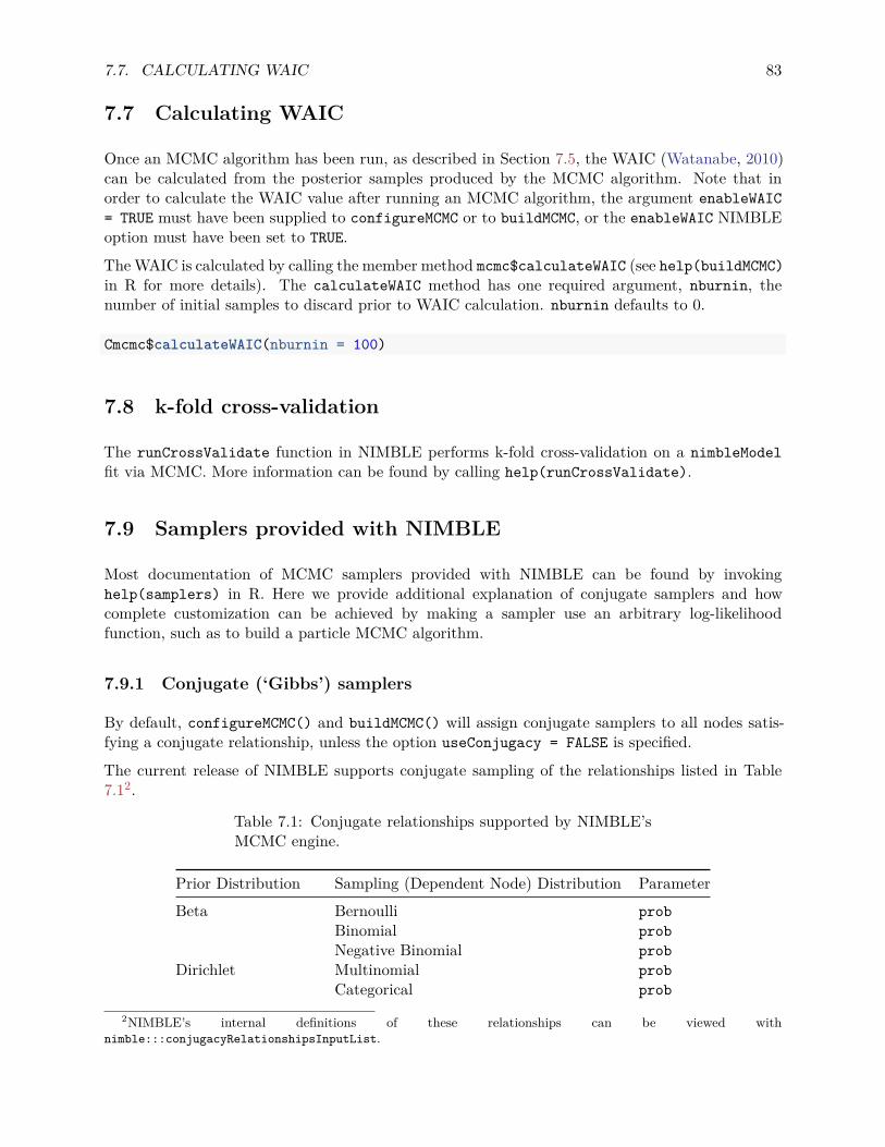
7.7. CALCULATING WAIC 83
7.7 Calculating WAIC
Once an MCMC algorithm has been run, as described in Section 7.5, the WAIC (Watanabe, 2010)can be calculated from the posterior samples produced by the MCMC algorithm. Note that inorder to calculate the WAIC value after running an MCMC algorithm, the argument enableWAIC= TRUE must have been supplied to configureMCMC or to buildMCMC, or the enableWAIC NIMBLEoption must have been set to TRUE.
The WAIC is calculated by calling the member method mcmc$calculateWAIC (see help(buildMCMC)in R for more details). The calculateWAIC method has one required argument, nburnin, thenumber of initial samples to discard prior to WAIC calculation. nburnin defaults to 0.
Cmcmc$calculateWAIC(nburnin = 100)
7.8 k-fold cross-validation
The runCrossValidate function in NIMBLE performs k-fold cross-validation on a nimbleModelfit via MCMC. More information can be found by calling help(runCrossValidate).
7.9 Samplers provided with NIMBLE
Most documentation of MCMC samplers provided with NIMBLE can be found by invokinghelp(samplers) in R. Here we provide additional explanation of conjugate samplers and howcomplete customization can be achieved by making a sampler use an arbitrary log-likelihoodfunction, such as to build a particle MCMC algorithm.
7.9.1 Conjugate (‘Gibbs’) samplers
By default, configureMCMC() and buildMCMC() will assign conjugate samplers to all nodes satis-fying a conjugate relationship, unless the option useConjugacy = FALSE is specified.
The current release of NIMBLE supports conjugate sampling of the relationships listed in Table7.12.
Table 7.1: Conjugate relationships supported by NIMBLE’sMCMC engine.
Prior Distribution Sampling (Dependent Node) Distribution ParameterBeta Bernoulli prob
Binomial probNegative Binomial prob
Dirichlet Multinomial probCategorical prob
2NIMBLE’s internal definitions of these relationships can be viewed withnimble:::conjugacyRelationshipsInputList.

84 CHAPTER 7. MCMC
Prior Distribution Sampling (Dependent Node) Distribution ParameterFlat Normal mean
Lognormal meanlogGamma Poisson lambda
Normal tauLognormal taulogGamma rateInverse Gamma scaleExponential rateWeibull lambda
Halfflat Normal sdLognormal sdlog
Inverse Gamma Normal varLognormal varlogGamma scaleInverse Gamma rateExponential scale
Normal Normal meanLognormal meanlog
Multivariate Normal Multivariate Normal meanWishart Multivariate Normal precInverse Wishart Multivariate Normal cov
Conjugate sampler functions may (optionally) dynamically check that their own posterior likelihoodcalculations are correct. If incorrect, a warning is issued. However, this functionality will roughlydouble the run-time required for conjugate sampling. By default, this option is disabled in NIMBLE.This option may be enabled with nimbleOptions(verifyConjugatePosteriors = TRUE).
If one wants information about conjugate node relationships for other purposes, they can be ob-tained using the checkConjugacy method on a model. This returns a named list describing allconjugate relationships. The checkConjugacy method can also accept a character vector argumentspecifying a subset of node names to check for conjugacy.
7.9.2 Customized log-likelihood evaluations: RW_llFunction sampler
Sometimes it is useful to control the log-likelihood calculations used for an MCMC updater insteadof simply using the model. For example, one could use a sampler with a log-likelihood that analyt-ically (or numerically) integrates over latent model nodes. Or one could use a sampler with a log-likelihood that comes from a stochastic approximation such as a particle filter (see below), allowingcomposition of a particle MCMC (PMCMC) algorithm (Andrieu et al., 2010). The RW_llFunctionsampler handles this by using a Metropolis-Hastings algorithm with a normal proposal distributionand a user-provided log-likelihood function. To allow compiled execution, the log-likelihood func-tion must be provided as a specialized instance of a nimbleFunction. The log-likelihood functionmay use the same model as the MCMC as a setup argument (as does the example below), butif so the state of the model should be unchanged during execution of the function (or you mustunderstand the implications otherwise).
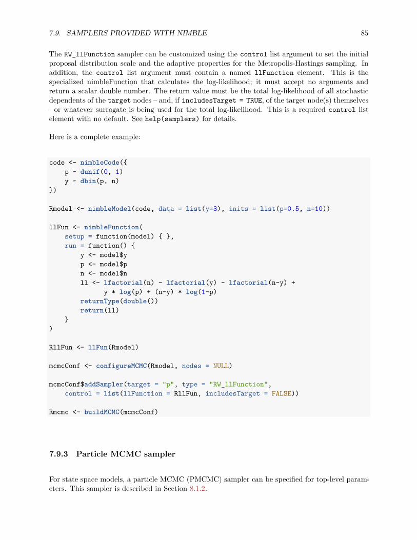
7.9. SAMPLERS PROVIDED WITH NIMBLE 85
The RW_llFunction sampler can be customized using the control list argument to set the initialproposal distribution scale and the adaptive properties for the Metropolis-Hastings sampling. Inaddition, the control list argument must contain a named llFunction element. This is thespecialized nimbleFunction that calculates the log-likelihood; it must accept no arguments andreturn a scalar double number. The return value must be the total log-likelihood of all stochasticdependents of the target nodes – and, if includesTarget = TRUE, of the target node(s) themselves– or whatever surrogate is being used for the total log-likelihood. This is a required control listelement with no default. See help(samplers) for details.
Here is a complete example:
code <- nimbleCode({p ~ dunif(0, 1)y ~ dbin(p, n)
})
Rmodel <- nimbleModel(code, data = list(y=3), inits = list(p=0.5, n=10))
llFun <- nimbleFunction(setup = function(model) { },run = function() {
y <- model$yp <- model$pn <- model$nll <- lfactorial(n) - lfactorial(y) - lfactorial(n-y) +
y * log(p) + (n-y) * log(1-p)returnType(double())return(ll)
})
RllFun <- llFun(Rmodel)
mcmcConf <- configureMCMC(Rmodel, nodes = NULL)
mcmcConf$addSampler(target = "p", type = "RW_llFunction",control = list(llFunction = RllFun, includesTarget = FALSE))
Rmcmc <- buildMCMC(mcmcConf)
7.9.3 Particle MCMC sampler
For state space models, a particle MCMC (PMCMC) sampler can be specified for top-level param-eters. This sampler is described in Section 8.1.2.

86 CHAPTER 7. MCMC
7.10 Detailed MCMC example: litters
Here is a detailed example of specifying, building, compiling, and running two MCMC algorithms.We use the litters example from the BUGS examples.
#################################### model configuration ####################################
# define our model using BUGS syntaxlitters_code <- nimbleCode({
for (i in 1:G) {a[i] ~ dgamma(1, .001)b[i] ~ dgamma(1, .001)for (j in 1:N) {
r[i,j] ~ dbin(p[i,j], n[i,j])p[i,j] ~ dbeta(a[i], b[i])
}mu[i] <- a[i] / (a[i] + b[i])theta[i] <- 1 / (a[i] + b[i])
}})
# list of fixed constantsconstants <- list(G = 2,
N = 16,n = matrix(c(13, 12, 12, 11, 9, 10, 9, 9, 8, 11, 8, 10, 13,
10, 12, 9, 10, 9, 10, 5, 9, 9, 13, 7, 5, 10, 7, 6,10, 10, 10, 7), nrow = 2))
# list specifying model datadata <- list(r = matrix(c(13, 12, 12, 11, 9, 10, 9, 9, 8, 10, 8, 9, 12, 9,
11, 8, 9, 8, 9, 4, 8, 7, 11, 4, 4, 5 , 5, 3, 7, 3,7, 0), nrow = 2))
# list specifying initial valuesinits <- list(a = c(1, 1),
b = c(1, 1),p = matrix(0.5, nrow = 2, ncol = 16),mu = c(.5, .5),theta = c(.5, .5))
# build the R model objectRmodel <- nimbleModel(litters_code,
constants = constants,data = data,inits = inits)
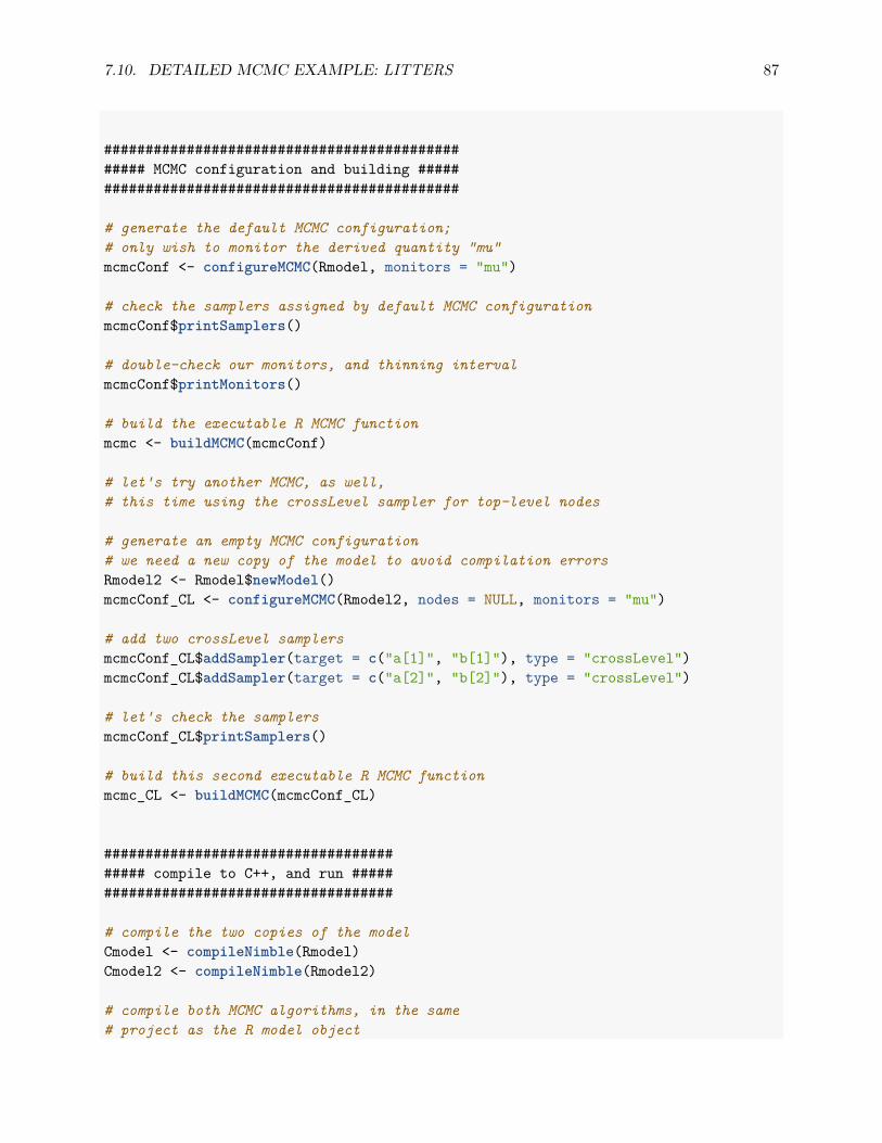
7.10. DETAILED MCMC EXAMPLE: LITTERS 87
################################################ MCMC configuration and building ################################################
# generate the default MCMC configuration;# only wish to monitor the derived quantity "mu"mcmcConf <- configureMCMC(Rmodel, monitors = "mu")
# check the samplers assigned by default MCMC configurationmcmcConf$printSamplers()
# double-check our monitors, and thinning intervalmcmcConf$printMonitors()
# build the executable R MCMC functionmcmc <- buildMCMC(mcmcConf)
# let's try another MCMC, as well,# this time using the crossLevel sampler for top-level nodes
# generate an empty MCMC configuration# we need a new copy of the model to avoid compilation errorsRmodel2 <- Rmodel$newModel()mcmcConf_CL <- configureMCMC(Rmodel2, nodes = NULL, monitors = "mu")
# add two crossLevel samplersmcmcConf_CL$addSampler(target = c("a[1]", "b[1]"), type = "crossLevel")mcmcConf_CL$addSampler(target = c("a[2]", "b[2]"), type = "crossLevel")
# let's check the samplersmcmcConf_CL$printSamplers()
# build this second executable R MCMC functionmcmc_CL <- buildMCMC(mcmcConf_CL)
######################################## compile to C++, and run ########################################
# compile the two copies of the modelCmodel <- compileNimble(Rmodel)Cmodel2 <- compileNimble(Rmodel2)
# compile both MCMC algorithms, in the same# project as the R model object
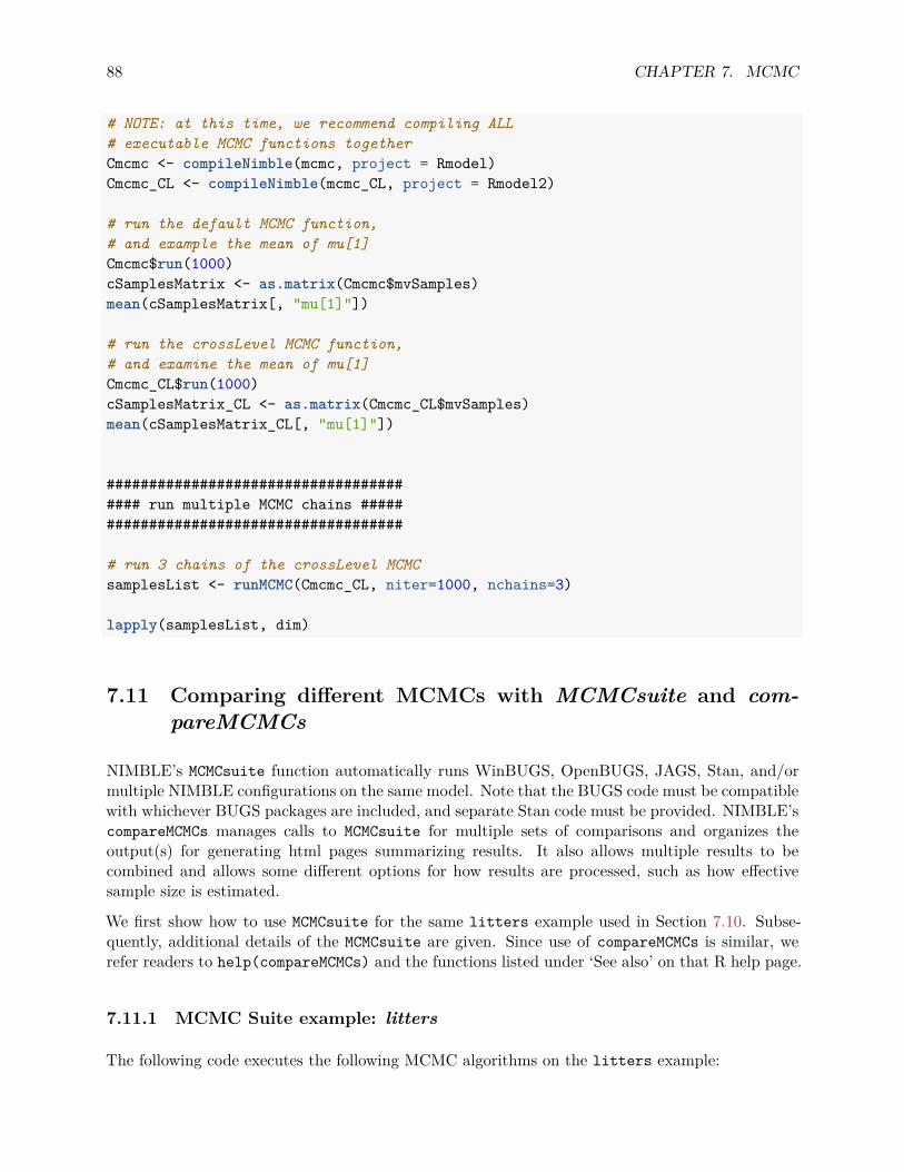
88 CHAPTER 7. MCMC
# NOTE: at this time, we recommend compiling ALL# executable MCMC functions togetherCmcmc <- compileNimble(mcmc, project = Rmodel)Cmcmc_CL <- compileNimble(mcmc_CL, project = Rmodel2)
# run the default MCMC function,# and example the mean of mu[1]Cmcmc$run(1000)cSamplesMatrix <- as.matrix(Cmcmc$mvSamples)mean(cSamplesMatrix[, "mu[1]"])
# run the crossLevel MCMC function,# and examine the mean of mu[1]Cmcmc_CL$run(1000)cSamplesMatrix_CL <- as.matrix(Cmcmc_CL$mvSamples)mean(cSamplesMatrix_CL[, "mu[1]"])
####################################### run multiple MCMC chains ########################################
# run 3 chains of the crossLevel MCMCsamplesList <- runMCMC(Cmcmc_CL, niter=1000, nchains=3)
lapply(samplesList, dim)
7.11 Comparing different MCMCs with MCMCsuite and com-pareMCMCs
NIMBLE’s MCMCsuite function automatically runs WinBUGS, OpenBUGS, JAGS, Stan, and/ormultiple NIMBLE configurations on the same model. Note that the BUGS code must be compatiblewith whichever BUGS packages are included, and separate Stan code must be provided. NIMBLE’scompareMCMCs manages calls to MCMCsuite for multiple sets of comparisons and organizes theoutput(s) for generating html pages summarizing results. It also allows multiple results to becombined and allows some different options for how results are processed, such as how effectivesample size is estimated.
We first show how to use MCMCsuite for the same litters example used in Section 7.10. Subse-quently, additional details of the MCMCsuite are given. Since use of compareMCMCs is similar, werefer readers to help(compareMCMCs) and the functions listed under ‘See also’ on that R help page.
7.11.1 MCMC Suite example: litters
The following code executes the following MCMC algorithms on the litters example:

7.11. COMPARING DIFFERENT MCMCS WITH MCMCSUITE AND COMPAREMCMCS 89
• WinBUGS• JAGS• NIMBLE default configuration• NIMBLE custom configuration using two crossLevel samplers
output <- MCMCsuite(code = litters_code,constants = constants,data = data,inits = inits,monitors = 'mu',MCMCs = c('winbugs', 'jags', 'nimble', 'nimble_CL'),MCMCdefs = list(
nimble_CL = quote({mcmcConf <- configureMCMC(Rmodel, nodes = NULL)mcmcConf$addSampler(target = c('a[1]', 'b[1]'),
type = 'crossLevel')mcmcConf$addSampler(target = c('a[2]', 'b[2]'),
type = 'crossLevel')mcmcConf
})),plotName = 'littersSuite'
)
7.11.2 MCMC Suite outputs
Executing the MCMC Suite returns a named list containing various outputs, as well as generatesand saves traceplots and posterior density plots. The default elements of this return list object are:
Samplessamples is a three-dimensional array, containing all MCMC samples from each algorithm. The firstdimension of the samples array corresponds to each MCMC algorithm, and may be indexed bythe name of the algorithm. The second dimension of the samples array corresponds to each nodewhich was monitored, and may be indexed by the node name. The third dimension of samplescontains the MCMC samples, and has length niter/thin - burnin.
SummaryThe MCMC suite output contains a variety of pre-computed summary statistics, which are storedin the summary matrix. For each monitored node and each MCMC algorithm, the following defaultsummary statistics are calculated: mean, median, sd, the 2.5% quantile, and the 97.5% quantile.These summary statistics are easily viewable, as:
output$summary# , , mu[1]# mean median sd quant025 quant975# winbugs 0.8795868 0.8889000 0.04349589 0.7886775 0.9205025# jags 0.8872778 0.8911989 0.02911325 0.8287991 0.9335317
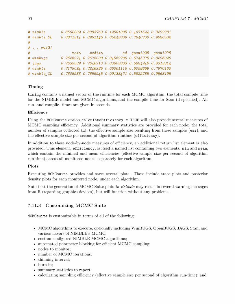
90 CHAPTER 7. MCMC
# nimble 0.8562232 0.8983763 0.12501395 0.4071524 0.9299781# nimble_CL 0.8871314 0.8961146 0.05243039 0.7640730 0.9620532## , , mu[2]# mean median sd quant025 quant975# winbugs 0.7626974 0.7678000 0.04569705 0.6745975 0.8296025# jags 0.7635539 0.7646913 0.03803033 0.6824946 0.8313314# nimble 0.7179094 0.7246935 0.06061116 0.6058669 0.7970130# nimble_CL 0.7605938 0.7655945 0.09138471 0.5822785 0.9568195
Timing
timing contains a named vector of the runtime for each MCMC algorithm, the total compile timefor the NIMBLE model and MCMC algorithms, and the compile time for Stan (if specified). Allrun- and compile- times are given in seconds.
Efficiency
Using the MCMCsuite option calculateEfficiency = TRUE will also provide several measures ofMCMC sampling efficiency. Additional summary statistics are provided for each node: the totalnumber of samples collected (n), the effective sample size resulting from these samples (ess), andthe effective sample size per second of algorithm runtime (efficiency).
In addition to these node-by-node measures of efficiency, an additional return list element is alsoprovided. This element, efficiency, is itself a named list containing two elements: min and mean,which contain the minimal and mean efficiencies (effective sample size per second of algorithmrun-time) across all monitored nodes, separately for each algorithm.
Plots
Executing MCMCsuite provides and saves several plots. These include trace plots and posteriordensity plots for each monitored node, under each algorithm.
Note that the generation of MCMC Suite plots in Rstudio may result in several warning messagesfrom R (regarding graphics devices), but will function without any problems.
7.11.3 Customizing MCMC Suite
MCMCsuite is customizable in terms of all of the following:
• MCMC algorithms to execute, optionally including WinBUGS, OpenBUGS, JAGS, Stan, andvarious flavors of NIMBLE’s MCMC;
• custom-configured NIMBLE MCMC algorithms;• automated parameter blocking for efficient MCMC sampling;• nodes to monitor;• number of MCMC iterations;• thinning interval;• burn-in;• summary statistics to report;• calculating sampling efficiency (effective sample size per second of algorithm run-time); and
7.11. COMPARING DIFFERENT MCMCS WITH MCMCSUITE AND COMPAREMCMCS 91
• generating and saving plots.
NIMBLE MCMC algorithms may be specified using the MCMCs argument to MCMCsuite, which ischaracter vector defining the MCMC algorithms to run. The MCMCs argument may include any ofthe following algorithms:
• “winbugs”: WinBUGS MCMC algorithm• “openbugs”: OpenBUGS MCMC algorithm• “jags”: JAGS MCMC algorithm• “Stan”: Stan default MCMC algorithm• “nimble”: NIMBLE MCMC using the default configuration• “nimble_noConj”: NIMBLE MCMC using the default configuration with useConjugacy =
FALSE• “autoBlock”: NIMBLE MCMC algorithm with block sampling of dynamically determined
parameter groups attempting to maximize sampling efficiency
The default value for the MCMCs argument is "nimble", which specifies only the default NIMBLEMCMC algorithm.
The names of additional, custom, MCMC algorithms may also be provided in the MCMCs argument,so long as these custom algorithms are defined in the MCMCdefs argument. An example of thisusage is given with the crossLevel algorithm in the litters example in 7.11.2.
The MCMCdefs argument should be a named list of definitions, for any custom MCMC algorithmsspecified in the MCMCs argument. If MCMCs specified an algorithm called "myMCMC", then MCMCdefsmust contain an element named "myMCMC". The contents of this element must be a block of codethat, when executed, returns the desired MCMC configuration object. This block of code mayassume the existence of the R model object, Rmodel. Further, this block of code need not worryabout adding monitors to the MCMC configuration; it need only specify the samplers.
As a final important point, execution of this block of code must return the MCMC configurationobject. Therefore, elements supplied in the MCMCdefs argument should usually take the form:
MCMCdefs = list(myMCMC = quote({
mcmcConf <- configureMCMC(Rmodel, ....)mcmcConf$addSampler(.....)mcmcConf # returns the MCMC configuration object
}))
Full details of the arguments and customization of the MCMC Suite is available viahelp(MCMCsuite).

92 CHAPTER 7. MCMC

Chapter 8
Sequential Monte Carlo and MCEM
The NIMBLE algorithm library is growing and as of version 0.6-7 includes a suite of SequentialMonte Carlo algorithms as well as a more robust MCEM and k-fold cross-validation.
8.1 Particle Filters / Sequential Monte Carlo
8.1.1 Filtering Algorithms
NIMBLE includes algorithms for four different types of sequential Monte Carlo (also known asparticle filters), which can be used to sample from the latent states and approximate the loglikelihood of a state space model. The particle filters currently implemented in NIMBLE are thebootstrap filter, the auxiliary particle filter, the Liu-West filter, and the ensemble Kalman filter,which can be built, respectively, with calls to buildBootstrapFilter, buildAuxiliaryFilter,buildLiuWestFilter, and buildEnsembleKF. Each particle filter requires setup arguments modeland nodes; the latter should be a character vector specifying latent model nodes. In addition, eachparticle filter can be customized using a control list argument. Details on the control options andspecifics of the filtering algorithms can be found in the help pages for the functions.
Once built, each filter can be run by specifying the number of particles. Each filter has a modelVal-ues object named mvEWSamples that is populated with equally-weighted samples from the posteriordistribution of the latent states (and in the case of the Liu-West filter, the posterior distribution ofthe top level parameters as well) as the filter is run. The bootstrap, auxiliary, and Liu-West filtersalso have another modelValues object, mvWSamples, which has unequally-weighted samples fromthe posterior distribution of the latent states, along with weights for each particle. In addition,the bootstrap and auxiliary particle filters return estimates of the log-likelihood of the given statespace model.
We first create a linear state-space model to use as an example for our particle filter algorithms.
# Building a simple linear state-space model.# x is latent space, y is observed datatimeModelCode <- nimbleCode({x[1] ~ dnorm(mu_0, 1)y[1] ~ dnorm(x[1], 1)
93

94 CHAPTER 8. SEQUENTIAL MONTE CARLO AND MCEM
for(i in 2:t){x[i] ~ dnorm(x[i-1] * a + b, 1)y[i] ~ dnorm(x[i] * c, 1)
}
a ~ dunif(0, 1)b ~ dnorm(0, 1)c ~ dnorm(1,1)mu_0 ~ dnorm(0, 1)
})
# simulate some datat <- 25; mu_0 <- 1x <- rnorm(1 ,mu_0, 1)y <- rnorm(1, x, 1)a <- 0.5; b <- 1; c <- 1for(i in 2:t){x[i] <- rnorm(1, x[i-1] * a + b, 1)y[i] <- rnorm(1, x[i] * c, 1)
}
# build the modelrTimeModel <- nimbleModel(timeModelCode, constants = list(t = t),
data <- list(y = y), check = FALSE )
# Set parameter values and compile the modelrTimeModel$a <- 0.5rTimeModel$b <- 1rTimeModel$c <- 1rTimeModel$mu_0 <- 1
cTimeModel <- compileNimble(rTimeModel)
Here is an example of building and running the bootstrap filter.
# Build bootstrap filterrBootF <- buildBootstrapFilter(rTimeModel, "x",
control = list(thresh = 0.8, saveAll = TRUE,smoothing = FALSE))
# Compile filtercBootF <- compileNimble(rBootF,project = rTimeModel)# Set number of particlesparNum <- 5000# Run bootstrap filter, which returns estimate of model log-likelihoodbootLLEst <- cBootF$run(parNum)# The bootstrap filter can also return an estimate of the effective# sample size (ESS) at each time point

8.1. PARTICLE FILTERS / SEQUENTIAL MONTE CARLO 95
bootESS <- cBootF$returnESS()
Next, we provide an example of building and running the auxiliary particle filter. Note that a filtercannot be built on a model that already has a filter specialized to it, so we create a new copy ofour state space model first.
# Copy our state-space model for use with the auxiliary filterauxTimeModel <- rTimeModel$newModel(replicate = TRUE)compileNimble(auxTimeModel)# Build auxiliary filterrAuxF <- buildAuxiliaryFilter(auxTimeModel, "x",
control = list(thresh = 0.5, saveAll = TRUE))# Compile filtercAuxF <- compileNimble(rAuxF,project = auxTimeModel)# Run auxiliary filter, which returns estimate of model log-likelihoodauxLLEst <- cAuxF$run(parNum)# The auxiliary filter can also return an estimate of the effective# sample size (ESS) at each time pointauxESS <- cAuxF$returnESS()
Now we give an example of building and running the Liu and West filter, which can sample fromthe posterior distribution of top-level parameters as well as latent states. The Liu and West filteraccepts an additional params argument, specifying the top-level parameters to be sampled.
# Copy modelLWTimeModel <- rTimeModel$newModel(replicate = TRUE)compileNimble(LWTimeModel)# Build Liu-West filter, also# specifying which top level parameters to estimaterLWF <- buildLiuWestFilter(LWTimeModel, "x", params = c("a", "b", "c"),
control = list(saveAll = FALSE))# Compile filtercLWF <- compileNimble(rLWF,project = LWTimeModel)# Run Liu-West filtercLWF$run(parNum)
Finally, we give an example of building and running the ensemble Kalman filter, which can samplefrom the posterior distribution of latent states.
# Copy modelENKFTimeModel <- rTimeModel$newModel(replicate = TRUE)compileNimble(ENKFTimeModel)# Build and compile ensemble Kalman filterrENKF <- buildEnsembleKF(ENKFTimeModel, "x",
control = list(saveAll = FALSE))cENKF <- compileNimble(rENKF,project = ENKFTimeModel)# Run ensemble Kalman filtercENKF$run(parNum)
96 CHAPTER 8. SEQUENTIAL MONTE CARLO AND MCEM
Once each filter has been run, we can extract samples from the posterior distribution of our latentstates as follows:
# Equally-weighted samples (available from all filters)bootEWSamp <- as.matrix(cBootF$mvEWSamples)auxEWSamp <- as.matrix(cAuxF$mvEWSamples)LWFEWSamp <- as.matrix(cLWF$mvEWSamples)ENKFEWSamp <- as.matrix(cENKF$mvEWSamples)
# Unequally-weighted samples, along with weights (available# from bootstrap, auxiliary, and Liu and West filters)bootWSamp <- as.matrix(cBootF$mvWSamples, "x")bootWts <- as.matrix(cBootF$mvWSamples, "wts")auxWSamp <- as.matrix(xAuxF$mvWSamples, "x")auxWts <- as.matrix(cAuxF$mvWSamples, "wts")
# Liu and West filter also returns samples# from posterior distribution of top-level parameters:aEWSamp <- as.matrix(cLWF$mvEWSamples, "a")
8.1.2 Particle MCMC (PMCMC)
Particle MCMC (PMCMC) is a method that uses MCMC for top-level model parameters and usesa particle filter to approximate the time-series likelihood for use in determining MCMC acceptanceprobabilities (Andrieu et al., 2010). NIMBLE implements PMCMC by providing random-walkMetropolis-Hastings samplers for model parameters that make use of particle filters in this way.These samplers can use NIMBLE’s bootstrap filter or auxiliary particle filter, or they can use auser-defined filter. Whichever filter is specified will be used to obtain estimates of the likelihoodof the state-space model (marginalizing over the latent states), which is used for calculation of theMetropolis-Hastings acceptance probability. The RW_PF sampler uses a univariate normal proposaldistribution, and can be used to sample scalar top-level parameters. The RW_PF_block sampleruses a multivariate normal proposal distribution and can be used to jointly sample vectors of top-level parameters. The PMCMC samplers can be specified with a call to addSampler with type= "RW_PF" or type = "RW_PF_block", a syntax similar to the other MCMC samplers listed inSection 7.9.
The RW_PF sampler and RW_PF_block sampler can be customized using the control list argumentto set the adaptive properties of the sampler and options for the particle filter algorithm to beused. In addition, providing pfOptimizeNparticles=TRUE in the control list will use an exper-imental algorithm to estimate the optimal number of particles to use in the particle filter. Seehelp(samplers) for details. The MCMC configuration for the timeModel in the previous sectionwill serve as an example for the use of our PMCMC sampler. Here we use the identity matrix asour proposal covariance matrix.
timeConf <- configureMCMC(rTimeModel) # default MCMC configuration
# Add random walk PMCMC sampler with particle number optimization.
8.2. MONTE CARLO EXPECTATION MAXIMIZATION (MCEM) 97
timeConf$addSampler(target = c("a", "b", "c", "mu_0"), type = "RW_PF_block",control <- list(propCov= diag(4), adaptScaleOnly = FALSE,
latents = "x", pfOptimizeNparticles = TRUE))
The type = "RW_PF" and type = "RW_PF_block" samplers default to using a bootstrap filter.However, more efficient results can often be obtained by using a custom filtering algorithm. Choiceof filtering algorithm can be controlled by the pfType control list entry. The pfType entry can be seteither to 'bootstrap' (the default), 'auxiliary', or the name of a user-defined nimbleFunctionthat returns a likelihood approximation.
Any user-defined filtering nimbleFunction named in the pfType control list entry must satsify thefollowing:
1. The nimbleFunction must be the result of a call to nimbleFunction().
2. The nimbleFunction must have setup code that accepts the following (and only the following)arguments:
• model, the NIMBLE model object that the MCMC algorithm is defined on.• latents, a character vector specifying the latent model nodes over which the particle
filter will stochastically integrate over to estimate the log-likelihood function.• control, an R list object. Note that the control list can be used to pass in any
additional information or arguments that the custom filter may require.
3. The nimbleFunction must have a run function that accepts a single integer arugment (thenumber of particles to use), and returns a scalar double (the log-likelihood estimate).
4. The nimbleFunction must define, in setup code, a modelValues object named mvEWSamplesthat is used to contain equally weighted samples of the latent states (that is, the latentsargument to the setup function). Each time the run() method of the nimbleFunction iscalled with number of particles m, the mvEWSamples modelValues object should be resized tobe of size m via a call to resize(mvEWSamples, m).
8.2 Monte Carlo Expectation Maximization (MCEM)
Suppose we have a model with missing data (or a layer of latent variables that can be treated asmissing data), and we would like to maximize the marginal likelihood of the model, integratingover the missing data. A brute-force method for doing this is MCEM. This is an EM algorithmin which the missing data are simulated via Monte Carlo (often MCMC, when the full conditionaldistributions cannot be directly sampled from) at each iteration. MCEM can be slow, and thereare other methods for maximizing marginal likelihoods that can be implemented in NIMBLE. Thereason we started with MCEM is to explore the flexibility of NIMBLE and illustrate the ability tocombine R and NIMBLE to run an algorithm, with R managing the highest-level processing of thealgorithm and calling nimbleFunctions for computations.
NIMBLE provides an ascent-based MCEM algorithm, created using buildMCEM, that automaticallydetermines when the algorithm has converged by examining the size of the changes in the likelihood

98 CHAPTER 8. SEQUENTIAL MONTE CARLO AND MCEM
between each iteration. Additionally, the MCEM algorithm can provide an estimate of the asymp-totic covariance matrix of the parameters. An example of calculating the asymptotic covariancecan be found in Section 8.2.1.We will revisit the pump example to illustrate the use of NIMBLE’s MCEM algorithm.
pump <- nimbleModel(code = pumpCode, name = "pump", constants = pumpConsts,data = pumpData, inits = pumpInits, check = FALSE)
compileNimble(pump)
# build an MCEM algorithm with ascent-based convergence criterionpumpMCEM <- buildMCEM(model = pump,
latentNodes = "theta", burnIn = 300,mcmcControl = list(adaptInterval = 100),boxConstraints = list( list( c("alpha", "beta"),
limits = c(0, Inf) ) ),buffer = 1e-6)
The first argument buildMCEM, model, is a NIMBLE model, which can be either the uncompiled orcompiled version. At the moment, the model provided cannot be part of another MCMC sampler.The ascent-based MCEM algorithm has a number of control options:The latentNodes argument should indicate the nodes that will be integrated over (sampled viaMCMC), rather than maximized. These nodes must be stochastic, not deterministic! latentNodeswill be expanded as described in Section 13.3.1.1. I.e., either latentNodes = "x" or latentNodes= c("x[1]", "x[2]") will treat x[1] and x[2] as latent nodes if x is a vector of two values. Allother non-data nodes will be maximized over. Note that latentNodes can include discrete nodes,but the nodes to be maximized cannot.The burnIn argument indicates the number of samples from the MCMC for the E-step that shouldbe discarded when computing the expected likelihood in the M-step. Note that burnIn can be setto values lower than in standard MCMC computations, as each iteration will start where the lastleft off.The mcmcControl argument will be passed to configureMCMC to define the MCMC to be used.The MCEM algorithm automatically detects box constraints for the nodes that will be optimized,using NIMBLE’s getBounds function. It is also possible for a user to manually specify constraintsvia the boxConstraints argument. Each constraint given should be a list in which the first elementis the names of the nodes or variables that the constraint will be applied to and the second elementis a vector of length two, in which the first value is the lower limit and the second is the upper limit.Values of Inf and -Inf are allowed. If a node is not listed, its constraints will be automaticallydetermined by NIMBLE. These constraint arguments are passed as the lower and upper argumentsto R’s optim function, using method = "L-BFGS-B". Note that NIMBLE will give a warning if auser-provided constraint is more extreme than the constraint determined by NIMBLE.The value of the buffer argument shrinks the boxConstraints by this amount. This can helpprotect against non-finite values occurring when a parameter is on the boundary.In addition, the MCEM has some extra control options that can be used to further tune theconvergence criterion. See help(buildMCEM) for more information.
8.2. MONTE CARLO EXPECTATION MAXIMIZATION (MCEM) 99
The buildMCEM function returns a list with two elements. The first element is a function calledrun, which will use the MCEM algorithm to estimate the MLEs. The second function is calledestimateCov, and is described in Section 8.2.1. The run function can be run as follows. Thereis only one run-time argument, initM, which is the number of MCMC iterations to use when thealgorithm is initialized.
pumpMLE <- pumpMCEM$run(initM = 1000)
## Iteration Number: 1.## Current number of MCMC iterations: 1000.## Parameter Estimates:## alpha beta## 0.8156929 1.1437769## Convergence Criterion: 1.001.## Iteration Number: 2.## Current number of MCMC iterations: 1000.## Parameter Estimates:## alpha beta## 0.8310559 1.2637092## Convergence Criterion: 0.02684197.## Monte Carlo error too big: increasing MCMC sample size.## Monte Carlo error too big: increasing MCMC sample size.## Iteration Number: 3.## Current number of MCMC iterations: 1875.## Parameter Estimates:## alpha beta## 0.8211969 1.2482232## Convergence Criterion: 0.001014128.## Monte Carlo error too big: increasing MCMC sample size.## Monte Carlo error too big: increasing MCMC sample size.## Monte Carlo error too big: increasing MCMC sample size.## Iteration Number: 4.## Current number of MCMC iterations: 5618.## Parameter Estimates:## alpha beta## 0.8219203 1.2552947## Convergence Criterion: 0.0002462065.
pumpMLE
## alpha beta## 0.8219203 1.2552947
Direct maximization after analytically integrating over the latent nodes (possible for this modelbut often not feasible) gives estimates of α̂ = 0.823 and β̂ = 1.261, so the MCEM seems to dopretty well, though tightening the convergence criteria may be warranted in actual usage.

100 CHAPTER 8. SEQUENTIAL MONTE CARLO AND MCEM
8.2.1 Estimating the Asymptotic Covariance From MCEM
The second element of the list returned by a call to buildMCEM is a function called estimateCov,which estimates the asymptotic covariance of the parameters at their MLE values. If the runfunction has been called previously, the estimateCov function will automatically use the MLEvalues produced by the run function to estimate the covariance. Alternatively, a user can supplytheir own MLE values using the MLEs argument, which allows the covariance to be estimatedwithout having called the run function. More details about the estimateCov function can befound by calling help(buildMCEM). Below is an example of using the estimateCov function.
pumpCov <- pumpMCEM$estimateCov()pumpCov
## alpha beta## alpha 0.1252970 0.2111132## beta 0.2111132 0.6160782
# Alternatively, you can manually specify the MLE values as a named vector.pumpCov <- pumpMCEM$estimateCov(MLEs = c(alpha = 0.823, beta = 1.261))

Chapter 9
Spatial models
NIMBLE supports two variations of conditional autoregressive (CAR) model structures: the im-proper intrinsic Gaussian CAR (ICAR) model, and a proper Gaussian CAR model. This includesdistributions to represent these spatially-dependent model structures in a BUGS model, as well asspecialized MCMC samplers for these distributions.
9.1 Intrinsic Gaussian CAR model: dcar_normal
The intrinsic Gaussian conditional autoregressive (ICAR) model used to model dependence of block-level values (e.g., spatial areas or temporal blocks) is implemented in NIMBLE as the dcar_normaldistribution. Additional details for using this distribution are available using help('CAR-Normal').
ICAR models are improper priors for random fields (e.g., temporal or spatial processes). Theprior is a joint prior across a collection of latent process values. For more technical details on CARmodels, including higher-order CAR models, please see Rue and Held (2005), Banerjee et al. (2015),and Paciorek (2009). Since the distribution is improper it should not be used as the distributionfor data values, but rather to specify a prior for an unknown process. As discussed in the referencesabove, the distribution can be seen to be a proper density in a reduced dimension subspace; thusthe impropriety only holds on one or more linear combinations of the latent process values.
In addition to our focus here on CAR modeling for spatial data, the ICAR model can also be usedin other contexts, such as for temporal data in a discrete time context.
9.1.1 Specification and density
NIMBLE uses the same parameterization as WinBUGS / GeoBUGS for the dcar_normal distribu-tion, providing compatibility with existing WinBUGS code. NIMBLE also provides the WinBUGSname car.normal as an alias.
9.1.1.1 Specification
The dcar_normal distribution is specified for a set of N spatially dependent regions as:
x[1:N] ~ dcar_normal(adj, weights, num, tau, c, zero_mean)
101

102 CHAPTER 9. SPATIAL MODELS
The adj, weights and num parameters define the adjacency structure and associated weights ofthe spatially-dependent field. See help('CAR-Normal') for details of these parameters. Whenspecifying a CAR distribution, these parameters must have constant values. They do not necessarilyhave to be specified as constants when creating a model object using nimbleModel, but theyshould be defined in a static way: as right-hand-side only variables with initial values provided asconstants, data or inits, or using fixed numerical deterministic declarations. Each of these twoapproaches for specifying values are shown in the example.The adjacency structure defined by adj and the associated weights must be symmetric. That is,if region i is neighbor of region j, then region j must also be a neighbor of region i. Further, theweights associated with these reciprocating relationships must be equal. NIMBLE performs a checkof these symmetries and will issue an error message if asymmetry is detected.The scalar precision tau may be treated as an unknown model parameter and itself assigned aprior distribution. Care should be taken in selecting a prior distribution for tau, and WinBUGSsuggests that users be prepared to carry out a sensitivity analysis for this choice.When specifying a higher-order CAR process, the number of constraints c can be explicitly providedin the model specification. This would be the case, for example, when specifying a thin-plate spline(second-order) CAR model, for which c should be 2 for a one-dimensional process and 3 for a two-dimensional (e.g., spatial) process, as discussed in Rue and Held (2005) and Paciorek (2009). If cis omitted, NIMBLE will calculate c as the number of disjoint groups of regions in the adjacencystructure, which implicitly assumes a first-order CAR process for each group.By default there is no zero-mean constraint imposed on the CAR process, and thus the mean isimplicit within the CAR process values, with an implicit improper flat prior on the mean. Toavoid non-identifiability, one should not include an additional parameter for the mean (e.g., donot include an intercept term in a simple CAR model with first-order neighborhood structure).When there are disjoint groups of regions and the constraint is not imposed, there is an implicitdistinct improper flat prior on the mean for each group, and it would not make sense to imposethe constraint since the constraint holds across all regions. Similarly, if one sets up a neighborhoodstructure for higher-order CAR models, it would not make sense to impose the zero-mean constraintas that would account for only one of the eigenvalues that are zero. Imposing this constraint (byspecifying the parameter zero_mean = 1) allows users to model the process mean separately, andhence a separate intercept term should be included in the model.NIMBLE provides a convenience function as.carAdjacency for converting other representations ofthe adjacency information into the required adj, weights, num format. This function can convert:
• A symmetric adjacency matrix of weights (with diagonal elements equal to zero), usingas.carAdjacency(weightMatrix)
• Two length-N lists with numeric vector elements giving the neighboring indices and associatedweights for each region, using as.carAdjacency(neighborList, weightList)
These conversions should be done in R, and the resulting adj, weights, num vectors can be passedas constants into nimbleModel.
9.1.1.2 Density
For process values x = (x1, . . . , xN ) and precision τ , the improper CAR density is given as:

9.1. INTRINSIC GAUSSIAN CAR MODEL: DCAR_NORMAL 103
p(x|τ) ∝ τ (N−c)/2 e− τ
2∑
i̸=jwij (xi−xj)2
where the summation over all (i, j) pairs, with the weight between regions i and j given by wij , isequivalent to summing over all pairs for which region i is a neighbor of region j. Note that thevalue of c modifies the power to which the precision is raised, accounting for the impropriety of thedensity based on the number of zero eigenvalues in the implicit precision matrix for x.For the purposes of MCMC sampling the individual CAR process values, the resulting conditionalprior of region i is:
p(xi|x−i, τ) ∼ N(
1wi+
∑j∈Ni
wij xj , wi+τ)
where x−i represents all elements of x except xi, the neighborhood Ni of region i is the set of allj for which region j is a neighbor of region i, wi+ =
∑j∈Ni
wij , and the Normal distribution isparameterized in terms of precision.
9.1.2 Example
Here we provide an example model using the intrinsic Gaussian dcar_normal distribution. TheCAR process values are used in a spatially-dependent Poisson regression.To mimic the behavior of WinBUGS, we specify zero_mean = 1 to enforce a zero-mean constrainton the CAR process, and therefore include a separate intercept term alpha in the model. Notethat we do not necessarily recommend imposing this constraint, per the discussion earlier in thischapter.
code <- nimbleCode({alpha ~ dflat()beta ~ dnorm(0, 0.0001)tau ~ dgamma(0.001, 0.001)for(k in 1:L)
weights[k] <- 1s[1:N] ~ dcar_normal(adj[1:L], weights[1:L], num[1:N], tau, zero_mean = 1)for(i in 1:N) {
log(lambda[i]) <- alpha + beta*x[i] + s[i]y[i] ~ dpois(lambda[i])
}})
constants <- list(N = 4, L = 8, num = c(3, 2, 2, 1),adj = c(2,3,4,1,3,1,2,1), x = c(0, 2, 2, 8))
data <- list(y = c(6, 9, 7, 12))inits <- list(alpha = 0, beta = 0, tau = 1, s = c(0, 0, 0, 0))Rmodel <- nimbleModel(code, constants, data, inits)
The resulting model may be carried through to MCMC sampling. NIMBLE will assign a specializedsampler to the update the elements of the CAR process. See Chapter 7 for information aboutNIMBLE’s MCMC engine, and Section 9.3 for details on MCMC sampling of the CAR processes.

104 CHAPTER 9. SPATIAL MODELS
9.2 Proper Gaussian CAR model: dcar_proper
The proper Gaussian conditional autoregressive model used to model dependence of block-levelvalues (e.g., spatial areas or temporal blocks) is implemented in NIMBLE as the dcar_properdistribution. Additional details of using this distribution are available using help('CAR-Proper').Proper CAR models are proper priors for random fields (e.g., temporal or spatial processes). Theprior is a joint prior across a collection of latent process values. For more technical details on properCAR models please see Banerjee et al. (2015), including considerations of why the improper CARmodel may be preferred.In addition to our focus here on CAR modeling for spatial data, the proper CAR model can alsobe used in other contexts, such as for temporal data in a discrete time context.
9.2.1 Specification and density
NIMBLE uses the same parameterization as WinBUGS / GeoBUGS for the dcar_proper distribu-tion, providing compatibility with existing WinBUGS code. NIMBLE also provides the WinBUGSname car.proper as an alias.
9.2.1.1 Specification
The dcar_proper distribution is specified for a set of N spatially dependent regions as:x[1:N] ~ dcar_proper(mu, C, adj, num, M, tau, gamma)
There is no option of a zero-mean constraint for proper CAR process, and instead the mean foreach region is specified by the mu parameter. The elements of mu can be assigned fixed values ormay be specified using one common, or multiple, prior distributions.The C, adj, num and M parameters define the adjacency structure, normalized weights, and con-ditional variances of the spatially-dependent field. See help('CAR-Proper') for details of theseparameters. When specifying a CAR distribution, these parameters must have constant values.They do not necessarily have to be specified as constants when creating a model object usingnimbleModel, but they should be defined in a static way: as right-hand-side only variables withinitial values provided as constants, data or inits, or using fixed numerical deterministic decla-rations.The adjacency structure defined by adj must be symmetric. That is, if region i is neighbor ofregion j, then region j must also be a neighbor of region i. In addition, the normalized weightsspecified in C must satisfy a symmetry constraint jointly with the conditional variances given inM. This constraint requires that M−1C is symmetric, where M is a diagonal matrix of conditionalvariances and C is the normalized (each row sums to one) weight matrix. Equivalently, this impliesthat CijMjj = CjiMii for all pairs of neighboring regions i and j. NIMBLE performs a check ofthese symmetries and will issue an error message if asymmetry is detected.Two options are available to simplify the process of constructing the C and M arguments; both optionsare demonstrated in the example. First, these arguments may be omitted from the dcar_properspecification. In this case, values of C and M will be generated that correspond to all weights beingequal to one, or equivalently, a symmetric weight matrix containing only zeros and ones. Note thatC and M should either both be provided, or both be omitted from the specification.

9.2. PROPER GAUSSIAN CAR MODEL: DCAR_PROPER 105
Second, a convenience function as.carCM is provided to generate the C and M arguments corre-sponding to a specified set of symmetric unnormalized weights. If weights contains the non-zeroweights corresponding to an unnormalized weight matrix (weights is precisely the argument thatcan be used in the dcar_normal specification), then a list containing C and M can be generatedusing as.carCM(adj, weights, num). In this case, the resulting C contains the row-normalizedweights, and the resulting M is a vector of the inverse row-sums of the unnormalized weight matrix.
The scalar precision tau may be treated as an unknown model parameter and itself assigned aprior distribution. Care should be taken in selecting a prior distribution for tau, and WinBUGSsuggests that users be prepared to carry out a sensitivity analysis for this choice.
An appropriate value of the gamma parameter ensures the propriety of the dcar_proper distribution.The value of gamma must lie between fixed bounds, which are given by the reciprocals of the largestand smallest eigenvalues of M−1/2CM1/2. These bounds can be calculated using the functioncarBounds or separately using the functions carMinBound and carMaxBound. For compatibilitywith WinBUGS, NIMBLE provides min.bound and max.bound as aliases for carMinBound andcarMaxBound. Rather than selecting a fixed value of gamma within these bounds, it is recommendedthat gamma be assigned a uniform prior distribution over the region of permissible values.
Note that when C and M are omitted from the dcar_proper specification (and hence all weights aretaken as one), or C and M are calculated from a symmetric weight matrix using the utility functionas.carCM, then the bounds on gamma are necessarily (−1, 1). In this case, gamma can simply beassigned a prior over that region. This approach is shown in both examples.
9.2.1.2 Density
The proper CAR density is given as:
p(x|µ, C, M, τ, γ) ∼ MVN(µ, 1
τ (I − γC)−1M)
where the multivariate normal distribution is parameterized in terms of covariance.
For the purposes of MCMC sampling the individual CAR process values, the resulting conditionalprior of region i is:
p(xi|x−i, µ, C, M, τ, γ) ∼ N(µi +
∑j∈Ni
γ Cij (xj − µi), Miiτ
)where x−i represents all elements of x except xi, the neighborhood Ni of region i is the set of all jfor which region j is a neighbor of region i, and the Normal distribution is parameterized in termsof variance.
9.2.2 Example
We provide two example models using the proper Gaussian dcar_proper distribution. In both,the CAR process values are used in a spatially-dependent logistic regression to model binary pres-ence/absence data. In the first example, the C and M parameters are omitted, which uses weightsequal to one for all neighbor relationships. In the second example, symmetric unnormalized weights

106 CHAPTER 9. SPATIAL MODELS
are specified, and as.carCM is used to construct the C and M parameters to the dcar_proper dis-tribution.
# omitting C and M sets all non-zero weights to onecode <- nimbleCode({
mu0 ~ dnorm(0, 0.0001)tau ~ dgamma(0.001, 0.001)gamma ~ dunif(-1, 1)s[1:N] ~ dcar_proper(mu[1:N], adj=adj[1:L], num=num[1:N], tau=tau,
gamma=gamma)for(i in 1:N) {
mu[i] <- mu0logit(p[i]) <- s[i]y[i] ~ dbern(p[i])
}})
adj <- c(2, 1, 3, 2, 4, 3)num <- c(1, 2, 2, 1)constants <- list(adj = adj, num = num, N = 4, L = 6)data <- list(y = c(1, 0, 1, 1))inits <- list(mu0 = 0, tau = 1, gamma = 0, s = rep(0, 4))Rmodel <- nimbleModel(code, constants, data, inits)
# specify symmetric unnormalized weights, use as.carCM to generate C and Mcode <- nimbleCode({
mu0 ~ dnorm(0, 0.0001)tau ~ dgamma(0.001, 0.001)gamma ~ dunif(-1, 1)s[1:N] ~ dcar_proper(mu[1:N], C[1:L], adj[1:L], num[1:N], M[1:N], tau,
gamma)for(i in 1:N) {
mu[i] <- mu0logit(p[i]) <- s[i]y[i] ~ dbern(p[i])
}})
weights <- c(2, 2, 3, 3, 4, 4)CM <- as.carCM(adj, weights, num)constants <- list(C = CM$C, adj = adj, num = num, M = CM$M, N = 4, L = 6)Rmodel <- nimbleModel(code, constants, data, inits)
Each of the resulting models may be carried through to MCMC sampling. NIMBLE will assigna specialized sampler to update the elements of the CAR process. See Chapter 7 for informationabout NIMBLE’s MCMC engine, and Section 9.3 for details on MCMC sampling of the CARprocesses.
9.3. MCMC SAMPLING OF CAR MODELS 107
9.3 MCMC Sampling of CAR models
NIMBLE’s MCMC engine provides specialized samplers for the dcar_normal and dcar_properdistributions. These samplers perform sequential univariate updates on the components of theCAR process. Internally, each sampler assigns one of three specialized univariate samplers to eachcomponent, based on inspection of the model structure:
1. A conjugate sampler in the case of conjugate Normal dependencies.2. A random walk Metropolis-Hastings sampler in the case of non-conjugate dependencies.3. A posterior predictive sampler in the case of no dependencies.
Note that these univariate CAR samplers are not the same as NIMBLE’s standard conjugate,RW, and posterior_predictive samplers, but rather specialized versions for operating on a CARdistribution. Details of these assignments are strictly internal to the CAR samplers.
In future versions of NIMBLE we expect to provide block samplers that update the entire CARprocess as a single sample. This may provide improved MCMC performance by accounting fordependence between elements, particularly when conjugacy is available.
9.3.1 Initial values
Valid initial values should be provided for all elements of the process specified by a CAR structurebefore running an MCMC. This ensures that the conditional prior distribution is well-defined foreach region. A simple and safe choice of initial values is setting all components of the process equalto zero, as is done in the preceding CAR examples.
For compatibility with WinBUGS, NIMBLE also allows an initial value of NA to be provided forregions with zero neighbors. This particular initialization is required in WinBUGS, so this allowsusers to make use of existing WinBUGS code.
9.3.2 Zero-neighbor regions
Regions with zero neighbors (defined by a 0 appearing in the num parameter) are a special casefor both the dcar_normal and dcar_proper distribution. The corresponding neighborhood N ofsuch a region contains no elements, and hence the conditional prior is improper and uninformative,tantamount to a dflat prior distribution. Thus, the conditional posterior distribution of thoseregions is entirely determined by the dependent nodes, if any. Sampling of these zero-neighborregions proceeds as:
1. In the conjugate case, sampling proceeds according to the conjugate posterior.2. In the non-conjugate case, sampling proceeds using random walk Metropolis-Hastings, where
the posterior is determined entirely by the dependencies.3. In the case of no dependents, the posterior is entirely undefined. Here, no changes will
be made to the process value, and it will remain equal to its initial value throughout. Byvirtue of having no neighbors, this region does not contribute to the density evaluation ofthe subsuming dcar_normal node nor to the conditional prior of any other regions, hence itsvalue (even NA) is of no consequence.

108 CHAPTER 9. SPATIAL MODELS
This behavior is different from that of WinBUGS, where the value of zero-neighbor regions ofcar.normal nodes is set to and fixed at zero.
9.3.3 Zero-mean constraint
A zero-mean constraint is available for the intrinsic Gaussian dcar_normal distribution. This con-straint on the ICAR process values is imposed during MCMC sampling, if the argument zero_mean= 1, mimicking the behavior of WinBUGS. Following the univariate updates on each component,the mean is subtracted away from all process values, resulting in a zero-mean process.
Note that this is not equivalent to sampling under the constraint that the mean is zero (see p. 36of Rue and Held (2005)) so should be treated as an ad hoc approach and employed with caution.

Chapter 10
Bayesian nonparametric models
As of version 0.6-11, NIMBLE provides initial support for Bayesian nonparametric (BNP) mixturemodeling. These features are currently considered EXPERIMENTAL – please let us know (via theNIMBLE user mailing list or by emailing us) if you have any problems or have suggestions aboutfunctionality you would like NIMBLE to support or the NIMBLE interface for using BNP.
10.1 Bayesian nonparametric mixture models
NIMBLE provides support for Bayesian nonparametric (BNP) mixture modeling. The currentimplementation provides support for hierarchical specifications involving Dirichlet process (DP)mixtures (Ferguson, 1973, 1974; Lo, 1984; Escobar, 1994; Escobar and West, 1995). More specifi-cally, a DP mixture model takes the form
yi | Giid∼
∫h(yi | θ)G(dθ),
G | α, G0 ∼ DP (α, G0),
where h(· | θ) is a suitable kernel with parameter θ, and α and G0 are the concentration andbaseline distribution parameters of the DP, respectively. DP mixture models can be written withdifferent levels of hierarchy, all being equivalent to the model above.
When the random measure G is integrated out from the model, the DP mixture model can bewritten using latent or membership variables, zi, following a Chinese Restaurant Process (CRP)distribution (Blackwell and MacQueen, 1973), discussed in Section 10.2. The model takes the form
yi | θ̃, ziind∼ h(· | θ̃zi),
z | α ∼ CRP(α), θ̃jiid∼ G0,
where CRP(α) denotes the CRP distribution with concentration parameter α.
If a stick-breaking representation (Sethuraman, 1994), discussed in section 10.3, is assumed for therandom measure G, then the model takes the form
109
110 CHAPTER 10. BAYESIAN NONPARAMETRIC MODELS
yi | θ⋆, vind∼
∞∑l=1
vl
∏m<l
(1 − vm)
h(· | θ⋆l ),
vl | αiid∼ Beta(1, α), θ⋆
liid∼ G0.
More general representations of the random measure can be specify by considering vl | νl, αlind∼
Beta(νl, αl). Finite dimensional approximations can be obtained by truncating the infinite sum tohave L components.
Different representations of DP mixtures lead to different computational algorithms. NIMBLEsupports sampling algorithms based on the CRP representation, as well as on the stick-breakingrepresentation. NIMBLE includes definitions of structures required to implement the CRP andstick-breaking distributions, and the associated MCMC algorithms.
10.2 Chinese Restaurant Process model
The CRP is a distribution over the space of partitions of positive integers and is implementedin NIMBLE as the dCRP distribution. More details for using this distribution are available usinghelp(CRP).
The CRP can be described as a stochastic process in which customers arrive at a restaurant,potentially with an infinite number of tables. Each customer sits at an empty or occupied tableaccording to probabilities that depend on the number of customers in the occupied tables. Thus,the CRP partitions the set of customers, through their assignment to tables in the restaurant.
10.2.1 Specification and density
NIMBLE parametrizes the dCRP distribution by a concentration parameter and a size parameter.
10.2.1.1 Specification
The dCRP distribution is specified in NIMBLE for a membership vector z as
z[1:N] ~ dCRP(conc, size)
The conc parameter is the concentration parameter of the CRP, controlling the probability of acustomer sitting on a new table, i.e., creating a new cluster. The size parameter defines the sizeof the set of integers to be partitioned.
The conc parameter is a positive real value that can be treated as known or unknown. When agamma prior is assumed for the conc parameter, a specialized sampler is assigned. See more onthis in section 10.4.1.
The size parameter is a positive integer that has to be fixed and equal to the length of vector z.It defines the set of consecutive integers from 1 to N to be partitioned. Each element in z can bean integer from 1 to N, and repetitions are allowed.

10.2. CHINESE RESTAURANT PROCESS MODEL 111
10.2.1.2 Density
The CRP distribution partitions the set of positive integers 1, . . . , N , into N⋆ ≤ N disjoint subsets,indicating to which subset each element belongs. For instance, if N = 6, the set {1, 2, 3, 4, 5, 6}can be partitioned into the subsets S1 = {1, 2, 6}, S2 = {4, 5}, and S3 = {3}. Note that N⋆ = 3,and this is one partition from out of 203 possibilities. The CRP-distributed vector z encodes thispartition and its observed values would be (1, 1, 3, 2, 2, 1), for this example. In mixture modeling,this indicates that observations 1, 2, and 6 belong to cluster 1, observations 4 and 5 to cluster 2,and observation 3 to cluster 3. Note that this representation is not unique, vector (2, 2, 1, 3, 3, 2)encodes the same partition.
The joint probability function of z = (z1, . . . , zN ), with concentration parameter α, is given by
p(z | α) ∝ Γ(α)Γ(α + n)
αN⋆(z)N⋆(z)∏k=1
Γ(mk(z)),
where mk(z) denotes the number of elements in z that are equal to k. The full conditional distri-bution for zi given z−i is
p(zi = m | z−i, α) = 1n − 1 + α
∑j ̸=i
1{zj}(m) + α
n − 1 + α1{znew}(m),
where z−i denotes vector z after removing its i−th component, znew is a value not in z−i, and 1A
denotes the indicator function at set A.
Note that the probability of creating a new cluster is proportional to α: the larger the concentrationparameter, the more clusters are created.
10.2.2 Example
The following example illustrates how to use NIMBLE to perform single density estimation for real-valued data, under a BNP approach, using the dCRP distribution. (Note that the BNP approach isalso often used to perform density estimation on random effects.) The model is given by
yi | θ̃, σ̃2, ziind∼ N(θ̃zi , σ̃2
zi, ) i = 1, . . . , N,
z ∼ CRP(α), α ∼ Gamma(1, 1),
θ̃jiid∼ N(0, 100), σ̃2
jiid∼ InvGamma(1, 1), j = 1, . . . , M.
code <- nimbleCode({z[1:N] ~ dCRP(alpha, size = N)alpha ~ dgamma(1, 1)for(i in 1:M) {
thetatilde[i] ~ dnorm(0, 100)s2tilde[i] ~ dinvgamma(1, 1)
}for(i in 1:N)
112 CHAPTER 10. BAYESIAN NONPARAMETRIC MODELS
y[i] ~ dnorm(thetatilde[z[i]], var = s2tilde[z[i]])})
set.seed(1)constants <- list(N = 100, M = 50)data <- list(y = c(rnorm(50, -5, sqrt(3)), rnorm(50, 5, sqrt(4))))inits <- list(thetatilde = rnorm(constants$N, 0, 10),
s2tilde = rinvgamma(constants$N, 1, 1),z = sample(1:10, size = constants$N, replace = TRUE),alpha = 1)
Rmodel <- nimbleModel(code, constants, data, inits)
The resulting model may be fitted through MCMC sampling. NIMBLE will assign a specializedsampler to update z and alpha. See Chapter 7 for information about NIMBLE’s MCMC engine,and Section 10.4.1 for details on MCMC sampling of the CRP.One of the advantages of BNP mixture models is that the number of clusters is treated as random.Therefore, in MCMC sampling, the number of cluster parameters varies with the iteration. SinceNIMBLE does not currently allow dynamic length allocation, the number of unique cluster param-eters, N⋆, has to be fixed. One safe option is to set this number to N , but this is inefficient, bothin terms of computation and in terms of storage, because in practice it is often that N⋆ < N . Inaddition, configuring and building the MCMC can be slow (and use a lot of memory) for large M .In an effort to mitigate these inefficiencies, we allow the user to set N⋆ = M , with M < N , asseen in the example above. However, if this number is too small and is exceeded in any iteration awarning is issued.
10.3 Stick-breaking model
In NIMBLE, weights defined by sequentially breaking a stick, as in the stick-breaking process,are implemented as the stick_breaking link function. More details for using this function areavailable using help(stick_breaking).
10.3.1 Specification and function
NIMBLE parametrizes the stick_breaking function by vector of values in (0, 1).
10.3.1.1 Function
The weights (w1, . . . , wL) follow a finite stick-breaking construction if
w1 = v1,
wl = vl
∏m<l
(1 − vm), l = 2, . . . , L − 1
wL =∏
m<L
(1 − vm).

10.3. STICK-BREAKING MODEL 113
for vl ∈ [0, 1], l = 1, . . . , L − 1.
10.3.1.2 Specification
The stick_breaking function is specified in NIMBLE for a vector w of probabilities as
w[1:L] <- stick_breaking(v[1:(L-1)])
The argument v is a vector of values between 0 and 1 defining the sequential breaking points ofthe stick after removing the previous portions already broken off. It is of length L − 1, implicitlyassuming that its last component is equal to 1.
In order to complete the definition of the weights in the stick-breaking representation of G, a priordistribution on (0, 1) should to be assumed for vl, l = 1, . . . , L − 1, for instance a beta prior.
10.3.2 Example
Here we illustrate how to use NIMBLE for the example described in section 10.2.2, but consideringa stick-breaking representation for G. The model is given by
yi | θ⋆, σ⋆2, ziind∼ N(θ⋆
zi , σ2⋆zi
), i = 1, . . . , N,
z ∼ Discrete(w), vliid∼ Beta(1, α), l = 1, . . . , L − 1,
α ∼ Gamma(1, 1),
θ⋆l
iid∼ N(0, 100), σ2⋆l
iid∼ InvGamma(1, 1), l = 1, . . . , L.
where w1 = v1, wl = vl∏
m<l(1 − vm), for l = 1, . . . , L − 1, and wL =∏
m<L(1 − vm).
code <- nimbleCode({for(i in 1:(L-1)){
v[i] ~ dbeta(1, alpha)}alpha ~ dgamma(1, 1)w[1:L] <- stick_breaking(v[1:(L-1)])for(i in 1:L) {
thetastar[i] ~ dnorm(0, 100)s2star[i] ~ dinvgamma(1, 1)
}for(i in 1:N) {
z[i] ~ dcat(w[1:L])y[i] ~ dnorm(thetastar[z[i]], var = s2star[z[i]])
}})
set.seed(1)constants <- list(N = 100, L=50)data <- list(y = c(rnorm(50, -5, sqrt(3)), rnorm(50, 5, sqrt(4))))
114 CHAPTER 10. BAYESIAN NONPARAMETRIC MODELS
inits <- list(thetastar = rnorm(constants$L, 0, 100),s2star = rinvgamma(constants$L, 1, 1),z = sample(1:10, size = constants$N, replace = TRUE),v = rbeta(constants$L, 1, 1),alpha = 1)
RmodelSB <- nimbleModel(code, constants, data, inits)
The resulting model may be carried through to MCMC sampling. NIMBLE will assign a specializedsampler to update v. See Chapter 7 for information about NIMBLE’s MCMC engine, and Section10.4.2 for details on MCMC sampling of the stick-breaking weights.
10.4 MCMC sampling of BNP models
BNP models can be specified in different, yet equivalent, manners. Examples 10.2.2 and 10.3.2are examples of density estimation for real-valued data, and are specified through the CRP andthe stick-breaking process, respectively. Different specifications lead NIMBLE to assign differentsampling algorithms for the model. When the model is specified through a CRP, a collapsed sampler(Neal, 2000) is assigned. Under this specification, the random measure G is integrated out fromthe model. When a stick-breaking representation is used, a blocked Gibbs sampler is assigned, seeIshwaran and James (2001) and Ishwaran and James (2002).
10.4.1 Sampling CRP models
NIMBLE’s MCMC engine provides specialized samplers for the dCRP distribution, updating eachcomponent of the membership vector sequentially. Internally, the sampler is assigned based oninspection of the model structure, evaluating conjugacy between the mixture kernel and the baselinedistribution, as follows:
1. A conjugate sampler in the case of the baseline distribution being conjugate for the mixturekernel.
2. A non-conjugate sampler in the case of the baseline distribution not being conjugate for themixture kernel.
Note that both samplers are specialized versions that operate on a vector having a CRP distribution.Details of these assignments are strictly internal to the CRP samplers. Additionally, a specializedsampler is assigned to the conc hyper parameter when a gamma hyper prior is assigned, see section6 in Escobar and West (1995) for more details. Otherwise, a random walk Metropolis-Hastingssampler is assigned.
10.4.1.1 Initial values
Valid initial values should be provided for all elements of the process specified by a CRP structurebefore running the MCMC. A simple and safe choice for z is to provide a sample of size N, the sameas its length, of values between 1 and some reasonable number of clusters (less than or equal tothe length of z), with replacement, as done in the preceding CRP example. For the concentrationparameter, a safe initial value is 1.

10.4. MCMC SAMPLING OF BNP MODELS 115
10.4.1.2 Sampling the random measure
In BNP models, it is oftenly of interest to make inference about the unknown measure G. NIMBLEprovides a sampler, getSamplesDPmeasure, for this random measure when a CRP structure isinvolved in the model.
The argument of the getsamplesDPmeasure function is a compiled or uncompiled MCMC object.The MCMC object should monitor the membership (clustering) variable, the cluster parameters,all stochastic nodes of the cluster parameters, and the concentration parameter, if it is random.Use the monitors argument when configuring the MCMC to ensure these variables are monitoredin the MCMC.
The sampler is used only after the MCMC for the model has been run; more details are availablefrom help(getsamplesDPmeasure).
The following code exemplifies how to generate samples from G after defining the model as inSection 10.2.2.
cRmodel <- compileNimble(Rmodel)
monitors <- c('z', 'thetatilde', 's2tilde' , 'alpha')RmodelConf <- configureMCMC(Rmodel, monitors = monitors)RmodelMCMC <- buildMCMC(RmodelConf)
CmodelMCMC <- compileNimble(RmodelMCMC, project = Rmodel)CmodelMCMC$run(1000)
samplesG <- getSamplesDPmeasure(CmodelMCMC)
10.4.2 Sampling stick-breaking models
NIMBLE’s MCMC engine provides specialized samplers for the beta-distributed random variablesthat are the arguments to the stick-breaking function, updating each component of the weight vectorsequentially. The sampler is assigned based on inspection of the model structure. Specifically, thespecialized sampler is assigned when the membership vector has a categorical distribution, itsweights are defined by a stick-breaking function, and the vector defining the weights follows a betadistribution.
10.4.2.1 Initial values
Valid initial values should be provided for all elements of the stick-breaking function and member-ship variable before running the MCMC. A simple and safe choice for z is to provide a sample ofsize N , of values between 1 and some value less than L, with replacement, as done in the precedingstick-breaking example. For the stick variables, safe initial values can be simulated from a betadistribution.

116 CHAPTER 10. BAYESIAN NONPARAMETRIC MODELS

Part IV
Programming with NIMBLE
117


119
Part IV is the programmer’s guide to NIMBLE. At the heart of programming in NIMBLE arenimbleFunctions. These support two principal features: (1) a setup function that is run once foreach model, nodes, or other setup arguments, and (2) run functions that will be compiled to C++and are written in a subset of R enhanced with features to operate models. Formally, what can becompiled comprises the NIMBLE language, which is designed to be R-like.
This part of the manual is organized as follows:
• Chapter 11 describes how to write simple nimbleFunctions, which have no setup code andhence don’t interact with models, to compile parts of R for fast calculations. This covers thesubset of R that is compilable, how to declare argument types and return types, and otherinformation.
• Chapter 12 explains how to write nimbleFunctions that can be included in BUGS code asuser-defined distributions or user-defined functions.
• Chapter 13 introduces more features of NIMBLE models that are useful for writing nimble-Functions to use models, focusing on how to query model structure and carry out modelcalculations.
• Chapter 14 introduces two kinds of data structures: modelValues are used for holding mul-tiple sets of values of model variables; nimbleList data structures are similar to R lists butrequire fixed element names and types, allowing the NIMBLE compiler to use them.
• Chapter 15 draws on the previous chapters to show how to write nimbleFunctions that workwith models, or more generally that have a setup function for any purpose. Typically asetup function queries model structure (Chapter 13) and may establish some modelValues ornimbleList data structures or configurations (Chapter 14). Then run functions written inthe same way as simple nimbleFunctions (Chapter 11) along with model operations (Chapter13) define algorithm computations that can be compiled via C++.

120
Chapter 11
Writing simple nimbleFunctions
11.1 Introduction to simple nimbleFunctions
nimbleFunctions are the heart of programming in NIMBLE. In this chapter, we introduce simplenimbleFunctions that contain only one function to be executed, in either compiled or uncompiledform, but no setup function or additional methods.
Defining a simple nimbleFunction is like defining an R function: nimbleFunction returns a functionthat can be executed, and it can also be compiled. Simple nimbleFunctions are useful for doingmath or the other kinds of processing available in NIMBLE when no model or modelValues isneeded. These can be used for any purpose in R programming. They can also be used as newfunctions and distributions in NIMBLE’s extension of BUGS (Chapter 12).
Here’s a basic example implementing the textbook calculation of least squares estimation of linearregression parameters1:
solveLeastSquares <- nimbleFunction(run = function(X = double(2), y = double(1)) { # type declarations
ans <- inverse(t(X) %*% X) %*% (t(X) %*% y)return(ans)returnType(double(2)) # return type declaration
} )
X <- matrix(rnorm(400), nrow = 100)y <- rnorm(100)solveLeastSquares(X, y)
## [,1]## [1,] 0.15448951## [2,] 0.02707736## [3,] -0.05432358## [4,] -0.05100693
1Of course, in general, explicitly calculating the inverse is not the recommended numerical recipe for least squares.
121

122 CHAPTER 11. WRITING SIMPLE NIMBLEFUNCTIONS
CsolveLeastSquares <- compileNimble(solveLeastSquares)CsolveLeastSquares(X, y)
## [,1]## [1,] 0.15448951## [2,] 0.02707736## [3,] -0.05432358## [4,] -0.05100693
In this example, we fit a linear model for 100 random response values (y) to four columns ofrandomly generated explanatory variables (X). We ran the nimbleFunction solveLeastSquaresuncompiled, natively in R, allowing testing and debugging (Section 15.7). Then we compiled it andshowed that the compiled version does the same thing, but faster2. NIMBLE’s compiler createsC++ that uses the Eigen (http://eigen.tuxfamily.org) library for linear algebra.
Notice that the actual NIMBLE code is written as an R function definition that is passed tonimbleFunction as the run argument. Hence we call it the run code. run code is written in theNIMBLE language. This is similar to a narrow subset of R with some additional features. Formally,we view it as a distinct language that encompasses what can be compiled from a nimbleFunction.
To write nimbleFunctions, you will need to learn:
• what R functions are supported for NIMBLE compilation and any ways they differ from theirregular R counterparts;
• how NIMBLE handles types of variables;• how to declare types of nimbleFunction arguments and return values;• that compiled nimbleFunctions always pass arguments to each other by reference.
The next sections cover each of these topics in turn.
11.2 R functions (or variants) implemented in NIMBLE
11.2.1 Finding help for NIMBLE’s versions of R functions
Often, R help pages are available for NIMBLE’s versions of R functions using the prefix ‘nim’ andcapitalizing the next letter. For example, help on NIMBLE’s version of numeric can be foundby help(nimNumeric). In some cases help is found directly using the name of the function as itappears in R.
11.2.2 Basic operations
Basic R operations supported for NIMBLE compilation are listed in Table 11.1.
2On the machine this is being written on, the compiled version runs a few times faster than the uncompiled version.However we refrain from formal speed tests.

11.2. R FUNCTIONS (OR VARIANTS) IMPLEMENTED IN NIMBLE 123
Table 11.1: Basic R manipulation functions in NIMBLE. Tofind help in R for NIMBLE’s version of a function, use the“nim” prefix and capitalize the next letter. E.g. help(nimC)for help with c().
Function Comments (differences from R)c() No recursive argument.rep() No rep.int or rep_len arguments.seq() and ‘:’ Negative integer sequences from ‘:’, e.g. , 2:1 do not work.which() No arr.ind or useNames arguments.diag() Works like R in three ways: diag(vector) returns a matrix with vector on the diagonal;
diag(matrix) returns the diagonal vector of matrix;diag(n) returns an n × n identity matrix. No nrow or ncol arguments.
diag()<- Works for assigning the diagonal vector of a matrix.dim() Works on a vector as well as higher-dimensional arguments.length()is.na() Does not correctly handle NAs from R that are type 'logical',
so convert these using as.numeric() before passing from R to NIMBLE.is.nan()numeric() Allows additional arguments to control initialization.logical() Allows additional arguments to control initialization.integer() Allows additional arguments to control initialization.matrix() Allows additional arguments to control initialization.array() Allows additional arguments to control initialization.indexing Arbitrary integer and logical indexing is supported for objects of one or two dimensions.
For higher-dimensional objects, only : indexing works and then only to create an objectof at most two dimensions.
Other R functions with numeric arguments and return value can be called during compiled executionby wrapping them as a nimbleRcall (see Section 11.7).Next we cover some of these functions in more detail.
11.2.2.1 numeric, integer, logical, matrix and array
numeric, integer, or logical will create a 1-dimensional vector of floating-point (or ‘double’[precision]), integer, or logical values, respectively. The length argument specifies the vector length(default 0), and the value argument specifies the initial value either as a scalar (used for all vectorelements, with default 0) or a vector. If a vector and its length is not equal to length, the remainingvalues will be zero, but we plan to implement R-style recycling in the next version of NIMBLE. Theinit argument specifies whether or not to initialize the elements in compiled code (default TRUE).If first use of the variable does not rely on initial values, using init = FALSE will yield slightlymore efficient performance.matrix creates a 2-dimensional matrix object of either floating-point (if type = "double", thedefault), integer (if type = "integer"), or logical (if type = "logical") values. As in R, nrowand ncol arguments specify the number of rows and columns, respectively. The value and initarguments are used in the same way as for numeric, integer, and logical.

124 CHAPTER 11. WRITING SIMPLE NIMBLEFUNCTIONS
array creates a vector or higher-dimensional object, depending on the dim argument, which takesa vector of sizes for each dimension. The type, value and init argument behave the same as formatrix.
The best way to create an identity matrix is with diag(n), which returns an n × n identity matrix.NIMBLE also provides a deprecated nimbleFunction identityMatrix that does the same thing.
Examples of these functions, and the related function ‘setSize‘ for changing the size of a numericobject, are given in Section 11.3.2.3.
11.2.2.2 length and dim
length behaves like R’s length function. It returns the entire length of X. That means if X ismultivariate, length(X) returns the product of the sizes of the dimensions. NIMBLE’s version ofdim, which has synonym nimDim, behaves like R’s dim function for matrices or arrays and like R’slength function for vectors. In other words, regardless of whether the number of dimensions is 1or more, it returns a vector of the sizes.
11.2.2.3 Deprecated creation of non-scalar objects using declare
Previous versions of NIMBLE provided a function declare for declaring variables. The more R-like functions numeric, integer, logical, matrix and array are intended to replace declare, butdeclare is still supported for backward compatibility. In a future version of NIMBLE, declaremay be removed.
11.2.3 Math and linear algebra
Numeric scalar and matrix mathematical operations are listed in Tables @ref{cha:RCfunctions}.2-@ref{cha:RCfunctions}.3.
As in R, many scalar operations in NIMBLE will work component-wise on vectors or higher dimen-sional objects. For example if B and C are vectors, A = B + C will add them and create vector Cby component-wise addition of B and C. In the current version of NIMBLE, component-wise opera-tions generally only work for vectors and matrices, not arrays with more than two dimensions. Theonly exception is assignment: A = B will work up to NIMBLE’s current limit of four dimensions.
Table 11.2: Functions operating on scalars, many of whichcan operate on each element (component-wise) of vectors andmatrices. Status column indicates if the function is currentlyprovided in NIMBLE. Vector input column indicates if thefunction can take a vector as an argument (i.e., if the functionis vectorized).
Usage Description Comments Status Vector inputx | y, x & y logical OR (|) and AND(&) yes yes!x logical not yes yesx > y, x >= y greater than (and or equal to) yes yesx < y, x <= y less than (and or equal to) yes yes

11.2. R FUNCTIONS (OR VARIANTS) IMPLEMENTED IN NIMBLE 125
Usage Description Comments Status Vector inputx != y, x == y (not) equals yes yesx + y, x - y, x * y component-wise operators mix of scalar and vector yes yesx / y component-wise division vector x and scalar y yes yesxˆy, pow(x, y) power xy; vector x,scalar y yes yesx %% y modulo (remainder) yes nomin(x1, x2), min. (max.) of two scalars yes See pmin,max(x1, x2) pmaxexp(x) exponential yes yeslog(x) natural logarithm yes yessqrt(x) square root yes yesabs(x) absolute value yes yesstep(x) step function at 0 0 if x < 0, 1 if x >= 0 yes yesequals(x) equality of two scalars 1 if x == y, 0 if x! = y yes yescube(x) third power x3 yes yessin(x), cos(x), trigonometric functions yes yestan(x)asin(x), acos(x), inverse trigonometric functions yes yesatan(x)asinh(x), acosh(x), inv. hyperbolic trig. functions yes yesatanh(x)logit(x) logit log(x/(1 − x)) yes yesilogit(x), expit(x) inverse logit exp(x)/(1 + exp(x)) yes yesprobit(x) probit (Gaussian quantile) Φ−1(x) yes yesiprobit(x), phi(x) inverse probit (Gaussian CDF) Φ(x) yes yescloglog(x) complementary log log log(− log(1 − x)) yes yesicloglog(x) inverse complementary log log 1 − exp(− exp(x)) yes yesceiling(x) ceiling function ⌈(x)⌉ yes yesfloor(x) floor function ⌊(x)⌋ yes yesround(x) round to integer yes yestrunc(x) truncation to integer yes yeslgamma(x), loggam(x) log gamma function log Γ(x) yes yesbesselK(k, nu, modified bessel function yes yes...expon.scaled) of the second kindlog1p(x) log of 1 + x log(1 + x) yes yeslfactorial(x), log factorial log x! yes yeslogfact(x)qDIST(x, PARAMS) “q” distribution functions canonical parameterization yes yespDIST(x, PARAMS) “p” distribution functions canonical parameterization yes yesrDIST(x, PARAMS) “r” distribution functions canonical parameterization yes yesdDIST(x, PARAMS) “d” distribution functions canonical parameterization yes yessort(x) norank(x, s) noranked(x, s) noorder(x) no
126 CHAPTER 11. WRITING SIMPLE NIMBLEFUNCTIONS
Table 11.3: Functions operating on vectors and matrices. Sta-tus column indicates if the function is currently provided inNIMBLE.
Usage Description Comments Statusinverse(x) matrix inverse x symmetric, positive def. yeschol(x) matrix Cholesky factorization x symmetric, positive def. yest(x) matrix transpose x⊤ yesx%*%y matrix multiply xy; x, y conformant yesinprod(x, y) dot product x⊤y; x and y vectors yessolve(x) solve system of equations x−1y; y matrix or vector yesforwardsolve(x, y) solve lower-triangular system of equations x−1y; x lower-triangular yesbacksolve(x, y) solve upper-triangular system of equations x−1y; x upper-triangular yeslogdet(x) log matrix determinant log |x| yesasRow(x) convert vector to 1-row matrix sometimes automatic yesasCol(x) convert vector to 1-column matrix sometimes automatic yessum(x) sum of elements of x yesmean(x) mean of elements of x yessd(x) standard deviation of elements of x yesprod(x) product of elements of x yesmin(x), max(x) min. (max.) of elements of x yespmin(x, y), pmax(x,y) vector of mins (maxs) of elements of yes
x and yinterp.lin(x, v1, v2) linear interpolation noeigen(x) matrix eigendecomposition; returns a x symmetric yes
nimbleList of type eigenNimbleListsvd(x) matrix singular value decomposition; yes
returns a nimbleList of typesvdNimbleList
More information on the nimbleLists returned by the eigen and svd functions in NIMBLE can befound in Section 14.2.1.
11.2.4 Distribution functions
Distribution ‘d’, ‘r’, ‘p’, and ‘q’ functions can all be used from nimbleFunctions (and in BUGSmodel code), but care is needed in the syntax, as follows.
• Names of the distributions generally (but not always) match those of R, which sometimesdiffer from BUGS. See the list below.
• Supported parameterizations are also indicated in the list below.• For multivariate distributions (multivariate normal, Dirichlet, and Wishart), ‘r’ functions only
return one random draw at a time, and the first argument must always be 1.• R’s recycling rule (re-use of an argument as needed to accommodate longer values of other
arguments) is generally followed, but the returned object is always a scalar or a vector, not amatrix or array.
11.2. R FUNCTIONS (OR VARIANTS) IMPLEMENTED IN NIMBLE 127
As in R (and nimbleFunctions), arguments are matched by order or by name (if given). Standardarguments to distribution functions in R (log, log.p, lower.tail) can be used and have the samedefaults. User-defined distributions for BUGS (Chapter 12) can also be used from nimbleFunctions.
For standard distributions, we rely on R’s regular help pages (e.g., help(dgamma). For distributionsunique to NIMBLE (e.g., dexp_nimble, ddirch), we provide help pages.
Supported distributions, listed by their ‘d’ function, include:
• dbinom(x, size, prob, log)• dcat(x, prob, log)• dmulti(x, size, prob, log)• dnbinom(x, size, prob, log)• dpois(x, lambda, log)• dbeta(x, shape1, shape2, log)• dchisq(x, df, log)• dexp(x, rate, log)• dexp_nimble(x, rate, log)• dexp_nimble(x, scale, log)• dgamma(x, shape, rate, log)• dgamma(x, shape, scale, log)• dinvgamma(x, shape, rate, log)• dinvgamma(x, shape, scale, log)• dlnorm(x, meanlog, sdlog, log)• dlogis(x, location, scale, log)• dnorm(x, mean, sd, log)• dt_nonstandard(x, df, mu, sigma, log)• dt(x, df, log)• dunif(x, min, max, log)• dweibull(x, shape, scale, log)• ddirch(x, alpha, log)• dmnorm_chol(x, mean, cholesky, prec_param, log)• dmvt_chol(x, mu, cholesky, df, prec_param, log)• dwish_chol(x, cholesky, df, scale_param, log)
In the last three, cholesky stands for Cholesky decomposition of the relevant matrix; prec_paramis a logical indicating whether the Cholesky is of a precision matrix (TRUE) or covariance matrix(FALSE)3; and scale_param is a logical indicating whether the Cholesky is of a scale matrix (TRUE)or an inverse scale matrix (FALSE).
11.2.5 Flow control: if-then-else, for, while, and stop
These basic flow-control structures use the same syntax as in R. However, for-loops are limited tosequential integer indexing. For example, for(i in 2:5) {...} works as it does in R. Decreasingindex sequences are not allowed. Unlike in R, if is not itself a function that returns a value.
3For the multivariate t, these are more properly termed the ‘inverse scale’ and ‘scale’ matrices
128 CHAPTER 11. WRITING SIMPLE NIMBLEFUNCTIONS
We plan to include more flexible for-loops in the future, but for now we’ve included justone additional useful feature: for(i in seq_along(NFL)) will work as in R, where NFL is animbleFunctionList. This is described in Section 15.4.8.
stop, or equivalently nimStop, throws control to R’s error-handling system and can take a characterargument that will be displayed in an error message.
11.2.6 print and cat
print, or equivalently nimPrint, prints an arbitrary set of outputs in order and adds a newlinecharacter at the end. cat or nimCat is identical, except without a newline at the end.
11.2.7 Checking for user interrupts: checkInterrupt
When you write algorithms that will run for a long time in C++, you may want to explicitly checkwhether a user has tried to interrupt the execution (i.e., by pressing Control-C). Simply includecheckInterrupt in run code at places where a check should be done. If there has been an interruptwaiting to be handled, the process will stop and return control to R.
11.2.8 Optimization: optim and nimOptim
NIMBLE provides a nimOptim function that partially implement’s R’s optim function with some mi-nor differences. nimOptim supports optimization methods ‘Nelder-Mead’, ‘BFGS’, ‘CG’, ‘L-BFGS-B’, but does not support methods ‘SANN’ and ‘Brent’. NIMBLE’s nimOptim supports gradientsusing user-provided functions if available or finite differences otherwise, but it does not currentlysupport Hessian computations. Currently nimOptim does not support extra parameters to thefunction being optimized (via \dots), but a work-around is to create a new nimbleFunction thatbinds those fixed parameters. Finally, nimOptim requires a nimbleList datatype for the controlparameter, whereas R’s optim uses a simple R list. To define the control parameter, create adefault value with the nimOptimDefaultControl function, and set any desired fields. For exampleusage, see the unit tests in tests/test-optim.R.
11.2.9 ‘nim’ synonyms for some functions
NIMBLE uses some keywords, such as dim and print, in ways similar but not identical to R. Inaddition, there are some keywords in NIMBLE that have the same names as R functions withquite different functionality. For example, step is part of the BUGS language, but it is also an Rfunction for stepwise model selection. And equals is part of the BUGS language but is also usedin the testthat package, which we use in testing NIMBLE.
NIMBLE tries to avoid conflicts by replacing some keywords immediately upon creating a nimble-Function. These replacements include
• c → nimC• copy → nimCopy• dim → nimDim

11.3. HOW NIMBLE HANDLES TYPES OF VARIABLES 129
• print → nimPrint• cat → nimCat• step → nimStep• equals → nimEquals• rep → nimRep• round → nimRound• seq → nimSeq• stop → nimStop• switch → nimSwitch• numeric, integer, logical → nimNumeric, nimInteger, nimLogical• matrix, array → nimMatrix, nimArray
This system gives programmers the choice between using the keywords like nimPrint directly, toavoid confusion in their own code about which ‘print’ is being used, or to use the more intuitivekeywords like print but remember that they are not the same as R’s functions.
11.3 How NIMBLE handles types of variables
Variables in the NIMBLE language are statically typed. Once a variable is used for one type, itcan’t subsequently be used for a different type. This rule facilitates NIMBLE’s compilation to C++.The NIMBLE compiler often determines types automatically, but sometimes the programmer needsto explicitly provide them.
The elemental types supported by NIMBLE include double (floating-point), integer, logical, andcharacter. The type of a numeric or logical object refers to the number of dimensions and theelemental type of the elements. Hence if x is created as a double matrix, it can only be usedsubsequently for a double matrix. The size of each dimension is not part of its type and thus canbe changed. Up to four dimensions are supported for double, integer, and logical. Only vectors(one dimension) are supported for character. Unlike R, NIMBLE supports true scalars, which have0 dimensions.
11.3.1 nimbleList data structures
A nimbleList is a data structure that can contain arbitrary other NIMBLE objects, includingother nimbleLists. Like other NIMBLE types, nimbleLists are strongly typed: each nimbleListis created from a configuration that declares what types of objects it will hold. nimbleLists arecovered in Chapter 14.2.
11.3.2 How numeric types work
R’s dynamic types support easy programming because one type can sometimes be transformedto another type automatically when an expression is evaluated. NIMBLE’s static types makes itstricter than R.
130 CHAPTER 11. WRITING SIMPLE NIMBLEFUNCTIONS
11.3.2.1 When NIMBLE can automatically set a numeric type
When a variable is first created by assignment, its type is determined automatically by that assign-ment. For example, if x has not appeared before, then
x <- A %*% B # assume A and B are double matrices or vectors
will create x to be a double matrix of the correct size (determined during execution). If x is usedsubsequently, it can only be used as a double matrix. This is true even if it is assigned a new value,which will again set its size automatically but cannot change its type.
11.3.2.2 When a numeric object needs to be created before being used
If the contents of a variable are to be populated by assignment into some indices in steps, thevariable must be created first. Further, it must be large enough for its eventual contents; it willnot be automatically resized if assignments are made beyond its current size. For example, in thefollowing code, x must be created before being filled with contents for specific indices.
x <- numeric(10)
for(i in 1:10)x[i] <- foo(y[i])
11.3.2.3 Changing the sizes of existing objects: setSize
setSize changes the size of an object, preserving its contents in column-major order.
# Example of creating and resizing a floating-point vector# myNumericVector will be of length 10, with all elements initialized to 2myNumericVector <- numeric(10, value = 2)# resize this numeric vector to be length 20; last 10 elements will be 0setSize(myNumericVector, 20)
# Example of creating a 1-by-10 matrix with values 1:10 and resizing itmyMatrix <- matrix(1:10, nrow = 1, ncol = 10)# resize this matrix to be a 10-by-10 matrixsetSize(myMatrix, c(10, 10))# The first column will have the 1:10
11.3.2.4 Confusions between scalars and length-one vectors
In R, there is no such thing is a true scalar; scalars can always be treated as vectors of length one.NIMBLE allows true scalars, which can create confusions. For example, consider the followingcode:
11.3. HOW NIMBLE HANDLES TYPES OF VARIABLES 131
myfun <- nimbleFunction(run = function(i = integer()) { # i is an integer scalar
randomValues <- rnorm(10) # double vectora <- randomValues[i] # double scalarb <- randomValues[i:i] # double vectord <- a + b # double vectorf <- c(i) # integer vector
})
In the line that creates b, the index range i:i is not evaluated until run time. Even though i:iwill always evaluate to simpy i, the compiler does not determine that. Since there is a vector indexrange provided, the result of randomValues[i:i] is determined to be a vector. The following linethen creates d as a vector, because a vector plus a scalar returns a vector. Another way to createa vector from a scalar is to use c, as illustrated in the last line.
11.3.2.5 Confusions between vectors and one-column or one-row matrices
Consider the following code:
myfun <- nimbleFunction(run = function() {
A <- matrix(value = rnorm(9), nrow = 3)B <- rnorm(3)Cmatrix <- A %*% B # double matrix, one columnCvector <- (A %*% B)[,1] # double vectorCmatrix <- (A %*% B)[,1] # error, vector assigned to matrixCmatrix[,1] <- (A %*% B)[,1] # ok, if Cmatrix is large enough
})
This creates a matrix A, a vector B, and matrix-multiplies them. The vector B is automaticallytreated as a one-column matrix in matrix algebra computations. The result of matrix multiplicationis always a matrix, but a programmer may expect a vector, since they know the result will haveone column. To make it a vector, simply extract the first column. More information about suchhandling is provided in the next section.
11.3.2.6 Understanding dimensions and sizes from linear algebra
As much as possible, NIMBLE behaves like R when determining types and sizes returned from linearalgebra expressions, but in some cases this is not possible because R uses run-time information whileNIMBLE must determine dimensions at compile time. For example, when matrix multiplying amatrix by a vector, R treats the vector as a one-column matrix unless treating it as a one-rowmatrix is the only way to make the expression valid, as determined at run time. NIMBLE usuallymust assume during compilation that it should be a one-column matrix, unless it can determinenot just the number of dimensions but the actual sizes during compilation. When needed asRowand asCol can control how a vector will be treated as a matrix.Here is a guide to such issues. Suppose v1 and v2 are vectors, and M1 is a matrix. Then

132 CHAPTER 11. WRITING SIMPLE NIMBLEFUNCTIONS
• v1 + M1 generates a compilation error unless one dimension of M1 is known at compile-timeto be 1. If so, then v1 is promoted to a 1-row or 1-column matrix to conform with M1, andthe result is a matrix of the same sizes. This behavior occurs for all component-wise binaryfunctions.
• v1 %*% M1 defaults to promoting v1 to a 1-row matrix, unless it is known at compile-timethat M1 has 1 row, in which case v1 is promoted to a 1-column matrix.
• M1 %*% v1 defaults to promoting v1 to a 1-column matrix, unless it is known at compile timethat M1 has 1 column, in which case v1 is promoted to a 1-row matrix.
• v1 %*% v2 promotes v1 to a 1-row matrix and v2 to a 1-column matrix, so the returnedvalues is a 1x1 matrix with the inner product of v1 and v2. If you want the inner product asa scalar, use inprod(v1, v2).
• asRow(v1) explicitly promotes v1 to a 1-row matrix. Therefore v1 %*% asRow(v2) gives theouter product of v1 and v2.
• asCol(v1) explicitly promotes v1 to a 1-column matrix.
• The default promotion for a vector is to a 1-column matrix. Therefore, v1 %*% t(v2) isequivalent to v1 %*% asRow(v2) .
• When indexing, dimensions with scalar indices will be dropped. For example, M1[1,] andM1[,1] are both vectors. If you do not want this behavior, use drop=FALSE just as in R. Forexample, M1[1,,drop=FALSE] is a matrix.
• The left-hand side of an assignment can use indexing, but if so it must already be correctlysized for the result. For example, Y[5:10, 20:30] <- x will not work – and could crashyour R session with a segmentation fault – if Y is not already at least 10x30 in size. Thiscan be done by setSize(Y, c(10, 30)). See Section 11.3.2.3 for more details. Note thatnon-indexed assignment to Y, such as Y <- x, will automatically set Y to the necessary size.
Here are some examples to illustrate the above points, assuming M2 is a square matrix.
• Y <- v1 + M2 %*% v2 will return a 1-column matrix. If Y is created by this statement, itwill be a 2-dimensional variable. If Y already exists, it must already be 2-dimesional, and itwill be automatically re-sized for the result.
• Y <- v1 + (M2 %*% v2)[,1] will return a vector. Y will either be created as a vector ormust already exist as a vector and will be re-sized for the result.
11.3.2.7 Size warnings and the potential for crashes
For matrix algebra, NIMBLE cannot ensure perfect behavior because sizes are not known untilrun time. Therefore, it is possible for you to write code that will crash your R session. In Version0.6-12, NIMBLE attempts to issue a warning if sizes are not compatible, but it does not haltexecution. Therefore, if you execute A <- M1 %*% M2, and M1 and M2 are not compatible for matrixmultiplication, NIMBLE will output a warning that the number of rows of M1 does not match thenumber of columns of M2. After that warning the statement will be executed and may result ina crash. Another easy way to write code that will crash is to do things like Y[5:10, 20:30] <-x without ensuring Y is at least 10x30. In the future we hope to prevent crashes, but in Version0.6-12 we limit ourselves to trying to provide useful information.
11.4. DECLARING ARGUMENT AND RETURN TYPES 133
11.4 Declaring argument and return types
NIMBLE requires that types of arguments and the type of the return value be explicitly declared.As illustrated in the example in Section 11.1, the syntax for a type declaration is:type(nDim, sizes)
where type is double, integer, logical or character. (In more general nimbleFunction program-ming, a type can also be a nimbleList type, discussed in Section 14.2.)For example run = function(x = double(1)) { ...} sets the single argument of the run functionto be a vector of numeric values of unknown size.For type(nDim, sizes), nDim is the number of dimensions, with 0 indicating scalar and omissionof nDim defaulting to a scalar. sizes is an optional vector of fixed, known sizes.For example, double(2, c(4, 5)) declares a 4 × 5 matrix. If sizes are omitted, they will be seteither by assignment or by setSize.In the case of scalar arguments only, a default value can be provided. For example, to provide 1.2as a default:
myfun <- nimbleFunction(run = function(x = double(0, default = 1.2)) {
})
Functions with return values must have their return type explicitly declared using returnType,which can occur anywhere in the run code. For example returnType(integer(2)) declares thereturn type to be a matrix of integers. A return type of void() means there is no return value,which is the default if no returnType statement is included.
11.5 Compiled nimbleFunctions pass arguments by reference
Uncompiled nimbleFunctions pass arguments like R does, by copy. If x is passed as an argumentto function foo, and foo modifies x internally, it is modifying its copy of x, not the original x thatwas passed to it.Compiled nimbleFunctions pass arguments to other compiled nimbleFunctions by reference (orpointer). This is very different. Now if foo modifies x internally, it is modifying the same x thatwas passed to it. This allows much faster execution but is obviously a fundamentally differentbehavior.Uncompiled execution of nimbleFunctions is primarily intended for debugging. However, debuggingof how nimbleFunctions interact via arguments requires testing the compiled versions.
11.6 Calling external compiled code
If you have a function in your own compiled C or C++ code and an appropriate header file, youcan generate a nimbleFunction that wraps access to that function, which can then be used in othernimbleFunctions. See help(nimbleExternalCall) for an example. This also contains an exampleof using an externally compiled function in the BUGS code of a model.

134 CHAPTER 11. WRITING SIMPLE NIMBLEFUNCTIONS
11.7 Calling uncompiled R functions from compiled nimbleFunc-tions
Sometimes one may want to combine R functions with compiled nimbleFunctions. Obviously acompiled nimbleFunction can be called from R. An R function with numeric inputs and output canbe called from compiled nimbleFunctions. The call to the R function is wrapped in a nimbleFunctionreturned by nimbleRcall. See help(nimbleRcall) for an example, including an example of usingthe resulting function in the BUGS code of a model.

Chapter 12
Creating user-defined BUGSdistributions and functions
NIMBLE allows you to define your own functions and distributions as nimbleFunctions for usein BUGS code. As a result, NIMBLE frees you from being constrained to the functions anddistributions discussed in Chapter 5. For example, instead of setting up a Dirichlet prior withmultinomial data and needing to use MCMC, one could recognize that this results in a Dirichlet-multinomial distribution for the data and provide that as a user-defined distribution instead.
Since NIMBLE allows you to wrap calls to external compiled code or arbitrary R functions asnimbleFunctions, and since you can define model functions and distributions as nimbleFunctions,you can combine these features to build external compiled code or arbitrary R functions into amodel. See Sections 11.6-11.7.
12.1 User-defined functions
To provide a new function for use in BUGS code, simply create a nimbleFunction that has no setupcode as discussed in Chapter 11. Then use it in your BUGS code. That’s it.
Writing nimbleFunctions requires that you declare the dimensionality of arguments and the returnedobject (Section 11.4). Make sure that the dimensionality specified in your nimbleFunction matcheshow you use it in BUGS code. For example, if you define scalar parameters in your BUGS code youwill want to define nimbleFunctions that take scalar arguments. Here is an example that returnstwice its input argument:
timesTwo <- nimbleFunction(run = function(x = double(0)) {
returnType(double(0))return(2*x)
})
code <- nimbleCode({for(i in 1:3) {
mu[i] ~ dnorm(0, 1)
135

136CHAPTER 12. CREATING USER-DEFINED BUGS DISTRIBUTIONS AND FUNCTIONS
mu_times_two[i] <- timesTwo(mu[i])}
})
The x = double(0) argument and returnType(double(0)) establish that the input and outputwill both be zero-dimensional (scalar) numbers.
You can define nimbleFunctions that take inputs and outputs with more dimensions. Here is anexample that takes a vector (1-dimensional) as input and returns a vector with twice the inputvalues:
vectorTimesTwo <- nimbleFunction(run = function(x = double(1)) {
returnType(double(1))return(2*x)
})
code <- nimbleCode({for(i in 1:3) {
mu[i] ~ dnorm(0, 1)}mu_times_two[1:3] <- vectorTimesTwo(mu[1:3])
})
There is a subtle difference between the mu_times_two variables in the two examples. In the firstexample, there are individual nodes for each mu_times_two[i]. In the second example, there isa single multivariate node, mu_times_two[1:3]. Each implementation could be more efficient fordifferent needs. For example, suppose an algorithm modifies the value of mu[2] and then updatesnodes that depend on it. In the first example, mu_times_two[2] would be updated. In the secondexample mu_times_two[1:3] would be updated because it is a single, vector node.
At present in compiled use of a model, you cannot provide a scalar argument where the user-definednimbleFunction expects a vector; unlike in R, scalars are not simply vectors of length 1.
12.2 User-defined distributions
To provide a user-defined distribution, you need to define density (‘d’) and simulation (‘r’)nimbleFunctions, without setup code, for your distribution. In some cases you can then simplyuse your distribution in BUGS code as you would any distribution already provided by NIMBLE,while in others you need to explicitly register your distribution as described in Section 12.2.1.
You can optionally provide distribution (‘p’) and quantile (‘q’) functions, which will allow trun-cation to be applied to a user-defined distribution. You can also provide a list of alternativeparameterizations, but only if you explicitly register the distribution.
Here is an extended example of providing a univariate exponential distribution (solely for illustrationas this is already provided by NIMBLE) and a multivariate Dirichlet-multinomial distribution.

12.2. USER-DEFINED DISTRIBUTIONS 137
dmyexp <- nimbleFunction(run = function(x = double(0), rate = double(0, default = 1),
log = integer(0, default = 0)) {returnType(double(0))logProb <- log(rate) - x*rateif(log) return(logProb)else return(exp(logProb))
})
rmyexp <- nimbleFunction(run = function(n = integer(0), rate = double(0, default = 1)) {
returnType(double(0))if(n != 1) print("rmyexp only allows n = 1; using n = 1.")dev <- runif(1, 0, 1)return(-log(1-dev) / rate)
})
pmyexp <- nimbleFunction(run = function(q = double(0), rate = double(0, default = 1),
lower.tail = integer(0, default = 1),log.p = integer(0, default = 0)) {returnType(double(0))if(!lower.tail) {
logp <- -rate * qif(log.p) return(logp)else return(exp(logp))
} else {p <- 1 - exp(-rate * q)if(!log.p) return(p)else return(log(p))
}})
qmyexp <- nimbleFunction(run = function(p = double(0), rate = double(0, default = 1),
lower.tail = integer(0, default = 1),log.p = integer(0, default = 0)) {returnType(double(0))if(log.p) p <- exp(p)if(!lower.tail) p <- 1 - preturn(-log(1 - p) / rate)
})
ddirchmulti <- nimbleFunction(run = function(x = double(1), alpha = double(1), size = double(0),
log = integer(0, default = 0)) {returnType(double(0))

138CHAPTER 12. CREATING USER-DEFINED BUGS DISTRIBUTIONS AND FUNCTIONS
logProb <- lgamma(size) - sum(lgamma(x)) + lgamma(sum(alpha)) -sum(lgamma(alpha)) + sum(lgamma(alpha + x)) - lgamma(sum(alpha) +
size)if(log) return(logProb)else return(exp(logProb))
})
rdirchmulti <- nimbleFunction(run = function(n = integer(0), alpha = double(1), size = double(0)) {
returnType(double(1))if(n != 1) print("rdirchmulti only allows n = 1; using n = 1.")p <- rdirch(1, alpha)return(rmulti(1, size = size, prob = p))
})
code <- nimbleCode({y[1:K] ~ ddirchmulti(alpha[1:K], n)for(i in 1:K) {
alpha[i] ~ dmyexp(1/3)}})
model <- nimbleModel(code, constants = list(K = 5, n = 10))
## Registering the following user-provided distributions: ddirchmulti .## NIMBLE has registered ddirchmulti as a distribution based on its use in BUGS code. Note that if you make changes to the nimbleFunctions for the distribution, you must call 'deregisterDistributions' before using the distribution in BUGS code for those changes to take effect.## Registering the following user-provided distributions: dmyexp .## NIMBLE has registered dmyexp as a distribution based on its use in BUGS code. Note that if you make changes to the nimbleFunctions for the distribution, you must call 'deregisterDistributions' before using the distribution in BUGS code for those changes to take effect.
The distribution-related functions should take as input the parameters for a single parameterization,which will be the canonical parameterization that NIMBLE will use.
Here are more details on the requirements for distribution-related nimbleFunctions, which followR’s conventions:
• Your distribution-related functions must have names that begin with ‘d’, ‘r’, ‘p’ and ‘q’. Thename of the distribution must not be identical to any of the NIMBLE-provided distributions.
• All simulation (‘r’) functions must take n as their first argument. Note that you may simplyhave your function only handle n=1 and return an warning for other values of n.
• NIMBLE uses doubles for numerical calculations, so we suggest simply using doubles ingeneral, even for integer-valued parameters or values of random variables.
• All density functions must have as their last argument log and implement return of the logprobability density. NIMBLE algorithms typically use only log = 1, but we recommend youimplement the log = 0 case for completeness.
• All distribution and quantile functions must have their last two arguments be (in order)lower.tail and log.p. These functions must work for lower.tail = 1 (i.e., TRUE) andlog.p = 0 (i.e., FALSE), as these are the inputs we use when working with truncated

12.2. USER-DEFINED DISTRIBUTIONS 139
distributions. It is your choice whether you implement the necessary calculations for othercombinations of these inputs, but again we recommend doing so for completeness.
• Define the nimbleFunctions in R’s global environment. Don’t expect R’s standard scoping towork1.
12.2.1 Using registerDistributions for alternative parameterizations and pro-viding other information
Behind the scenes, NIMBLE uses the function registerDistributions to set up new distributionsfor use in BUGS code. In some circumstances, you will need to call registerDistributionsdirectly to provide information that NIMBLE can’t obtain automatically from the nimbleFunctionsyou write.
The cases in which you’ll need to explicitly call registerDistributions are when you want to doany of the following:
• provide alternative parameterizations,• indicate a distribution is discrete, and• provide the range of possible values for a distribution.
If you would like to allow for multiple parameterizations, you can do this via the Rdist elementof the list provided to registerDistributions as illustrated below. If you provide CDF (‘p’)and inverse CDF (quantile, i.e. ‘q’) functions, be sure to specify pqAvail = TRUE when youcall registerDistributions. Here’s an example of using registerDistributions to provide analternative parameterization (scale instead of rate) and to provide the range for the user-definedexponential distribution. We can then use the alternative parameterization in our BUGS code.
registerDistributions(list(dmyexp = list(
BUGSdist = "dmyexp(rate, scale)",Rdist = "dmyexp(rate = 1/scale)",altParams = c("scale = 1/rate", "mean = 1/rate"),pqAvail = TRUE,range = c(0, Inf))
))
## Registering the following user-provided distributions: dmyexp .## Overwriting the following user-supplied distributions: dmyexp .
code <- nimbleCode({y[1:K] ~ ddirchmulti(alpha[1:K], n)for(i in 1:K) {
alpha[i] ~ T(dmyexp(scale = 3), 0, 100)
1NIMBLE can’t use R’s standard scoping because it doesn’t work for R reference classes, and nimbleFunctionsare implemented as custom-generated reference classes.

140CHAPTER 12. CREATING USER-DEFINED BUGS DISTRIBUTIONS AND FUNCTIONS
}})
model <- nimbleModel(code, constants = list(K = 5, n = 10),inits = list(alpha = rep(1, 5)))
There are a few rules for how you specify the information about a distribution that you provide toregisterDistributions:
• The function name in the BUGSdist entry in the list provided to registerDistributionswill be the name you can use in BUGS code.
• The names of your nimbleFunctions must match the function name in the Rdist entry. Ifmissing, the Rdist entry defaults to be the same as the BUGSdist entry.
• Your distribution-related functions must take as arguments the parameters in default order,starting as the second argument and in the order used in the parameterizations in the Rdistargument to registerDistributions or the BUGSdist argument if there are no alternativeparameterizations.
• You must specify a types entry in the list provided to registerDistributions if the distri-bution is multivariate or if any parameter is non-scalar.
Further details on using registerDistributions can be found via R help on registerDistributions.NIMBLE uses the same list format as registerDistributions to define its distributions. Thislist can be found in the R/distributions_inputList.R file in the package source code directoryor as the R list nimble:::distributionsInputList.

Chapter 13
Working with NIMBLE models
Here we describe how one can get information about NIMBLE models and carry out operations ona model. While all of this functionality can be used from R, its primary use occurs when writingnimbleFunctions (see Chapter 15). Information about node types, distributions, and dimensionscan be used to determine algorithm behavior in setup code of nimbleFunctions. Information aboutnode or variable values or the parameter and bound values of a node would generally be used foralgorithm calculations in run code of nimbleFunctions. Similarly, carrying out numerical operationson a model, including setting node or variable values, would generally be done in run code.
13.1 The variables and nodes in a NIMBLE model
Section 6.2 defines what we mean by variables and nodes in a NIMBLE model and discusses how todetermine and access the nodes in a model and their dependency relationships. Here we’ll reviewand go into more detail on the topics of determining the nodes and node dependencies in a model.
13.1.1 Determining the nodes in a model
One can determine the variables in a model using getVarNames and the nodes in a model usinggetNodeNames, with optional arguments allowing you to select only certain types of nodes. Weillustrate here with the pump model from Chapter 2.
pump$getVarNames()
## [1] "lifted_d1_over_beta" "theta" "lambda"## [4] "x" "alpha" "beta"
pump$getNodeNames()
## [1] "alpha" "beta" "lifted_d1_over_beta"## [4] "theta[1]" "theta[2]" "theta[3]"## [7] "theta[4]" "theta[5]" "theta[6]"
141

142 CHAPTER 13. WORKING WITH NIMBLE MODELS
## [10] "theta[7]" "theta[8]" "theta[9]"## [13] "theta[10]" "lambda[1]" "lambda[2]"## [16] "lambda[3]" "lambda[4]" "lambda[5]"## [19] "lambda[6]" "lambda[7]" "lambda[8]"## [22] "lambda[9]" "lambda[10]" "x[1]"## [25] "x[2]" "x[3]" "x[4]"## [28] "x[5]" "x[6]" "x[7]"## [31] "x[8]" "x[9]" "x[10]"
pump$getNodeNames(determOnly = TRUE)
## [1] "lifted_d1_over_beta" "lambda[1]" "lambda[2]"## [4] "lambda[3]" "lambda[4]" "lambda[5]"## [7] "lambda[6]" "lambda[7]" "lambda[8]"## [10] "lambda[9]" "lambda[10]"
pump$getNodeNames(stochOnly = TRUE)
## [1] "alpha" "beta" "theta[1]" "theta[2]" "theta[3]"## [6] "theta[4]" "theta[5]" "theta[6]" "theta[7]" "theta[8]"## [11] "theta[9]" "theta[10]" "x[1]" "x[2]" "x[3]"## [16] "x[4]" "x[5]" "x[6]" "x[7]" "x[8]"## [21] "x[9]" "x[10]"
pump$getNodeNames(dataOnly = TRUE)
## [1] "x[1]" "x[2]" "x[3]" "x[4]" "x[5]" "x[6]" "x[7]" "x[8]"## [9] "x[9]" "x[10]"
You can see one lifted node (see next section), lifted_d1_over_beta, involved in a reparameteri-zation to NIMBLE’s canonical parameterization of the gamma distribution for the theta nodes.
We can determine the set of nodes contained in one or more nodes or variables us-ing expandNodeNames, illustrated here for an example with multivariate nodes. ThereturnScalarComponents argument also allows us to return all of the scalar elements ofmultivariate nodes.
multiVarCode2 <- nimbleCode({X[1, 1:5] ~ dmnorm(mu[], cov[,])X[6:10, 3] ~ dmnorm(mu[], cov[,])for(i in 1:4)
Y[i] ~ dnorm(mn, 1)})
multiVarModel2 <- nimbleModel(multiVarCode2,
13.1. THE VARIABLES AND NODES IN A NIMBLE MODEL 143
dimensions = list(mu = 5, cov = c(5,5)),calculate = FALSE)
multiVarModel2$expandNodeNames("Y")
## [1] "Y[1]" "Y[2]" "Y[3]" "Y[4]"
multiVarModel2$expandNodeNames(c("X", "Y"), returnScalarComponents = TRUE)
## [1] "X[1, 1]" "X[1, 2]" "X[1, 3]" "X[6, 3]" "X[7, 3]" "X[8, 3]"## [7] "X[9, 3]" "X[10, 3]" "X[1, 4]" "X[1, 5]" "Y[1]" "Y[2]"## [13] "Y[3]" "Y[4]"
As discussed in Section 6.2.6, you can determine whether a node is flagged as data using isData.
13.1.2 Understanding lifted nodes
In some cases, NIMBLE introduces new nodes into the model that were not specified in the BUGScode for the model, such as the lifted_d1_over_beta node in the introductory example. For thisreason, it is important that programs written to adapt to different model structures use NIMBLE’ssystems for querying the model graph. For example, a call to pump$getDependencies("beta")will correctly include lifted_d1_over_beta in the results. If one skips this step and assumes thenodes are only those that appear in the BUGS code, one may not get correct results.
It can be helpful to know the situations in which lifted nodes are generated. These include:
1. When distribution parameters are expressions, NIMBLE creates a new deterministic nodethat contains the expression for a given parameter. The node is then a direct descendantof the new deterministic node. This is an optional feature, but it is currently enabled in allcases.
2. As discussed in Section 5.2.6, the use of link functions causes new nodes to be introduced.This requires care if you need to initialize values in stochastic declarations with link functions.
3. Use of alternative parameterizations of distributions, described in Section 5.2.4 causes newnodes to be introduced. For example when a user provides the precision of a normal distri-bution as tau, NIMBLE creates a new node sd <- 1/sqrt(tau) and uses sd as a parameterin the normal distribution. If many nodes use the same tau, only one new sd node will becreated, so the computation 1/sqrt(tau) will not be repeated redundantly.
13.1.3 Determining dependencies in a model
Next we’ll see how to determine the node dependencies (or ‘descendants’) in a model. Thereare a variety of arguments to getDependencies that allow one to specify whether to include thenode itself, whether to include deterministic or stochastic or data dependents, etc. By defaultgetDependencies returns descendants up to the next stochastic node on all edges emanating from

144 CHAPTER 13. WORKING WITH NIMBLE MODELS
the node(s) specified as input. This is what would be needed to calculate a Metropolis-Hastingsacceptance probability in MCMC, for example.
pump$getDependencies("alpha")
## [1] "alpha" "theta[1]" "theta[2]" "theta[3]" "theta[4]"## [6] "theta[5]" "theta[6]" "theta[7]" "theta[8]" "theta[9]"## [11] "theta[10]"
pump$getDependencies(c("alpha", "beta"))
## [1] "alpha" "beta" "lifted_d1_over_beta"## [4] "theta[1]" "theta[2]" "theta[3]"## [7] "theta[4]" "theta[5]" "theta[6]"## [10] "theta[7]" "theta[8]" "theta[9]"## [13] "theta[10]"
pump$getDependencies("theta[1:3]", self = FALSE)
## [1] "lambda[1]" "lambda[2]" "lambda[3]" "x[1]" "x[2]" "x[3]"
pump$getDependencies("theta[1:3]", stochOnly = TRUE, self = FALSE)
## [1] "x[1]" "x[2]" "x[3]"
# get all dependencies, not just the direct descendantspump$getDependencies("alpha", downstream = TRUE)
## [1] "alpha" "theta[1]" "theta[2]" "theta[3]" "theta[4]"## [6] "theta[5]" "theta[6]" "theta[7]" "theta[8]" "theta[9]"## [11] "theta[10]" "lambda[1]" "lambda[2]" "lambda[3]" "lambda[4]"## [16] "lambda[5]" "lambda[6]" "lambda[7]" "lambda[8]" "lambda[9]"## [21] "lambda[10]" "x[1]" "x[2]" "x[3]" "x[4]"## [26] "x[5]" "x[6]" "x[7]" "x[8]" "x[9]"## [31] "x[10]"
pump$getDependencies("alpha", downstream = TRUE, dataOnly = TRUE)
## [1] "x[1]" "x[2]" "x[3]" "x[4]" "x[5]" "x[6]" "x[7]" "x[8]"## [9] "x[9]" "x[10]"

13.2. ACCESSING INFORMATION ABOUT NODES AND VARIABLES 145
13.2 Accessing information about nodes and variables
13.2.1 Getting distributional information about a node
We briefly demonstrate some of the functionality for information about a node here, but referreaders to the R help on modelBaseClass for full details.
Here is an example model, with use of various functions to determine information about nodes orvariables.
code <- nimbleCode({for(i in 1:4)
y[i] ~ dnorm(mu, sd = sigma)mu ~ T(dnorm(0, 5), -20, 20)sigma ~ dunif(0, 10)})
m <- nimbleModel(code, data = list(y = rnorm(4)),inits = list(mu = 0, sigma = 1))
m$isEndNode('y')
## y[1] y[2] y[3] y[4]## TRUE TRUE TRUE TRUE
m$getDistribution('sigma')
## sigma## "dunif"
m$isDiscrete(c('y', 'mu', 'sigma'))
## y[1] y[2] y[3] y[4] mu sigma## FALSE FALSE FALSE FALSE FALSE FALSE
m$isDeterm('mu')
## mu## FALSE
m$getDimension('mu')
## value## 0
146 CHAPTER 13. WORKING WITH NIMBLE MODELS
m$getDimension('mu', includeParams = TRUE)
## value mean sd tau var## 0 0 0 0 0
Note that any variables provided to these functions are expanded into their constituent node names,so the length of results may not be the same length as the input vector of node and variable names.However the order of the results should be preserved relative to the order of the inputs, once theexpansion is accounted for.
13.2.2 Getting information about a distribution
One can also get generic information about a distribution based on the name of the distributionusing the function getDistributionInfo. In particular, one can determine whether a distributionwas provided by the user (isUserDefined), whether a distribution provides CDF and quantilefunctions (pqDefined), whether a distribution is a discrete distribution (isDiscrete), the param-eter names (include alternative parameterizations) for a distribution (getParamNames), and thedimension of the distribution and its parameters (getDimension). For more extensive information,please see the R help for getDistributionInfo.
13.2.3 Getting distribution parameter values for a node
The function getParam provides access to values of the parameters of a node’s distribution.getParam can be used as global function taking a model as the first argument, or it can be usedas a model member function. The next two arguments must be the name of one (stochastic) nodeand the name of a parameter for the distribution followed by that node. The parameter does nothave to be one of the parameters used when the node was declared. Alternative parameterizationvalues can also be obtained. See Section 5.2.4.1 for available parameterizations. (These can alsobe seen in nimble:::distributionsInputList.)Here is an example:
gammaModel <- nimbleModel(nimbleCode({
a ~ dlnorm(0, 1)x ~ dgamma(shape = 2, scale = a)
}), data = list(x = 2.4), inits = list(a = 1.2))getParam(gammaModel, 'x', 'scale')
## [1] 1.2
getParam(gammaModel, 'x', 'rate')
## [1] 0.8333333

13.2. ACCESSING INFORMATION ABOUT NODES AND VARIABLES 147
gammaModel$getParam('x','rate')
## [1] 0.8333333
getParam is part of the NIMBLE language, so it can be used in run code of nimbleFunctions.
13.2.4 Getting distribution bounds for a node
The function getBound provides access to the lower and upper bounds of the distribution for a node.In most cases these bounds will be fixed based on the distribution, but for the uniform distributionthe bounds are the parameters of the distribution, and when truncation is used (Section 5.2.7),the bounds will be determined by the truncation. Like the functions described in the previoussection, getBound can be used as global function taking a model as the first argument, or it can beused as a model member function. The next two arguments must be the name of one (stochastic)node and either "lower" or "upper" indicating whether the lower or upper bound is desired. Formultivariate nodes the bound is a scalar that is the bound for all elements of the node, as we donot handle truncation for multivariate nodes.Here is an example:
exampleModel <- nimbleModel(nimbleCode({
y ~ T(dnorm(mu, sd = sig), a, Inf)a ~ dunif(-1, b)b ~ dgamma(1, 1)
}), inits = list(a = -0.5, mu = 1, sig = 1, b = 4),data = list(y = 4))
getBound(exampleModel, 'y', 'lower')
## [1] -0.5
getBound(exampleModel, 'y', 'upper')
## [1] Inf
exampleModel$b <- 3exampleModel$calculate(exampleModel$getDependencies('b'))
## [1] -4.386294
getBound(exampleModel, 'a', 'upper')
## [1] 3
148 CHAPTER 13. WORKING WITH NIMBLE MODELS
exampleModel$getBound('b','lower')
## [1] 0
getBound is part of the NIMBLE language, so it can be used in run code of nimbleFunctions. Infact, we anticipate that most use of getBound will be for algorithms, such as for the reflectionversion of the random walk MCMC sampler.
13.3 Carrying out model calculations
13.3.1 Core model operations: calculation and simulation
The four basic ways to operate a model are to calculate nodes, simulate into nodes, get the logprobabilities (or probability densities) that have already been calculated, and compare the logprobability of a new value to that of an old value. In more detail:
• calculate For a stochastic node, calculate determines the log probability value, stores itin the appropriate logProb variable, and returns it. For a deterministic node, calculateexecutes the deterministic calculation and returns 0.
• simulate For a stochastic node, simulate generates a random draw. For deterministic nodes,simulate is equivalent to calculate without returning 0. simulate always returns NULL (orvoid in C++).
• getLogProb getLogProb simply returns the most recently calculated log probability value,or 0 for a deterministic node.
• calculateDiff calculateDiff is identical to calculate, but it returns the new log prob-ability value minus the one that was previously stored. This is useful when one wants tochange the value or values of node(s) in the model (e.g., by setting a value or simulate) andthen determine the change in the log probability, such as needed for a Metropolis-Hastingsacceptance probability.
Each of these functions is accessed as a member function of a model object, taking a vector of nodenames as an argument1. If there is more than one node name, calculate and getLogProb returnthe sum of the log probabilities from each node, while calculateDiff returns the sum of the newvalues minus the old values. Next we show an example using simulate.
13.3.1.1 Example: simulating arbitrary collections of nodes
mc <- nimbleCode({a ~ dnorm(0, 0.001)for(i in 1:5) {
y[i] ~ dnorm(a, 0.1)
1Standard usage is model$calculate(nodes) but calculate(model, nodes) is synonymous.
13.3. CARRYING OUT MODEL CALCULATIONS 149
for(j in 1:3)z[i,j] ~ dnorm(y[i], sd = 0.1)
}y.squared[1:5] <- y[1:5]^2
})
model <- nimbleModel(mc, data = list(z = matrix(rnorm(15), nrow = 5)))
model$a <- 1model$y
## [1] NA NA NA NA NA
model$simulate("y[1:3]")# simulate(model, "y[1:3]")model$y
## [1] -5.5477219 10.6631058 0.1735369 NA NA
model$simulate("y")model$y
## [1] -0.4369177 1.4982502 3.9516343 1.9576271 -5.1858901
model$z
## [,1] [,2] [,3]## [1,] -1.26959907 1.8001123 2.2363228## [2,] 2.34949332 1.0114402 0.3022651## [3,] -1.41200541 -0.5637166 -1.0425066## [4,] -0.01696149 0.2054208 -0.9835423## [5,] -0.54431935 1.1654620 2.0057186
model$simulate(c("y[1:3]", "z[1:5, 1:3]"))model$y
## [1] 2.117981 2.424367 3.085683 1.957627 -5.185890
model$z
## [,1] [,2] [,3]## [1,] -1.26959907 1.8001123 2.2363228## [2,] 2.34949332 1.0114402 0.3022651## [3,] -1.41200541 -0.5637166 -1.0425066## [4,] -0.01696149 0.2054208 -0.9835423## [5,] -0.54431935 1.1654620 2.0057186
150 CHAPTER 13. WORKING WITH NIMBLE MODELS
model$simulate(c("z[1:5, 1:3]"), includeData = TRUE)model$z
## [,1] [,2] [,3]## [1,] 2.014839 1.880879 2.085524## [2,] 2.329938 2.347778 2.328989## [3,] 3.045883 3.054561 3.165292## [4,] 2.056270 1.878174 1.926745## [5,] -5.149746 -5.046011 -5.191497
The example illustrates a number of features:
1. simulate(model, nodes) is equivalent to model$simulate(nodes). You can use either, butthe latter is encouraged and the former may be deprecated inthe future.
2. Inputs like "y[1:3]" are automatically expanded into c("y[1]", "y[2]", "y[3]"). In fact,simply "y" will be expanded into all nodes within y.
3. An arbitrary number of nodes can be provided as a character vector.4. Simulations will be done in the order provided, so in practice the nodes should often be
obtained by functions such as getDependencies. These return nodes in topologically-sortedorder, which means no node is manipulated before something it depends on.
5. The data nodes z were not simulated into until includeData = TRUE was used.
Use of calculate, calculateDiff and getLogProb are similar to simulate, except that theyreturn a value (described above) and they have no includeData argument.
13.3.2 Pre-defined nimbleFunctions for operating on model nodes: simNodes,calcNodes, and getLogProbNodes
simNodes, calcNodes and getLogProbNodes are basic nimbleFunctions that simulate, calculate, orget the log probabilities (densities), respectively, of the same set of nodes each time they are called.Each of these takes a model and a character string of node names as inputs. If nodes is left blank,then all the nodes of the model are used.
For simNodes, the nodes provided will be topologically sorted to simulate in the correct order. ForcalcNodes and getLogProbNodes, the nodes will be sorted and dependent nodes will be included.Recall that the calculations must be up to date (from a calculate call) for getLogProbNodes toreturn the values you are probably looking for.
simpleModelCode <- nimbleCode({for(i in 1:4){
x[i] ~ dnorm(0,1)y[i] ~ dnorm(x[i], 1) # y depends on xz[i] ~ dnorm(y[i], 1) # z depends on y# z conditionally independent of x
}})

13.3. CARRYING OUT MODEL CALCULATIONS 151
simpleModel <- nimbleModel(simpleModelCode, check = FALSE)cSimpleModel <- compileNimble(simpleModel)
# simulates all the x's and y'srSimXY <- simNodes(simpleModel, nodes = c('x', 'y') )
# calls calculate on x and its dependents (y, but not z)rCalcXDep <- calcNodes(simpleModel, nodes = 'x')
# calls getLogProb on x's and y'srGetLogProbXDep <- getLogProbNodes(simpleModel,
nodes = 'x')
# compiling the functionscSimXY <- compileNimble(rSimXY, project = simpleModel)cCalcXDep <- compileNimble(rCalcXDep, project = simpleModel)cGetLogProbXDep <- compileNimble(rGetLogProbXDep, project = simpleModel)
cSimpleModel$x
## [1] NA NA NA NA
cSimpleModel$y
## [1] NA NA NA NA
# simulating x and ycSimXY$run()
## NULL
cSimpleModel$x
## [1] -1.6988735 0.2318525 -0.1190907 1.7724929
cSimpleModel$y
## [1] -1.3554513 -0.3911972 -0.5586130 1.2671961
cCalcXDep$run()
## [1] -10.87675

152 CHAPTER 13. WORKING WITH NIMBLE MODELS
# gives correct answer because logProbs# updated by 'calculate' after simulationcGetLogProbXDep$run()
## [1] -10.87675
cSimXY$run()
## NULL
# gives old answer because logProbs# not updated after 'simulate'cGetLogProbXDep$run()
## [1] -10.87675
cCalcXDep$run()
## [1] -8.568001
13.3.3 Accessing log probabilities via logProb variables
For each variable that contains at least one stochastic node, NIMBLE generates a model variablewith the prefix ‘logProb_’. In general users will not need to access these logProb variables directlybut rather will use getLogProb. However, knowing they exist can be useful, in part because thesevariables can be monitored in an MCMC.
When the stochastic node is scalar, the logProb variable will have the same size. For example:
model$logProb_y
## [1] NA NA NA NA NA
model$calculate("y")
## [1] -12.69171
model$logProb_y
## [1] -2.132725 -2.171672 -2.287735 -2.116084 -3.983493

13.3. CARRYING OUT MODEL CALCULATIONS 153
Creation of logProb variables for stochastic multivariate nodes is trickier, because they can repre-sent an arbitrary block of a larger variable. In general NIMBLE records the logProb values usingthe lowest possible indices. For example, if x[5:10, 15:20] follows a Wishart distribution, itslog probability (density) value will be stored in logProb_x[5, 15]. When possible, NIMBLE willreduce the dimensions of the corresponding logProb variable. For example, in
for(i in 1:10) x[i,] ~ dmnorm(mu[], prec[,])
x may be 10 × 20 (dimensions must be provided), but logProb_x will be 10 × 1. For the most partyou do not need to worry about how NIMBLE is storing the log probability values, because youcan always get them using getLogProb.

154 CHAPTER 13. WORKING WITH NIMBLE MODELS

Chapter 14
Data structures in NIMBLE
NIMBLE provides several data structures useful for programming.
We’ll first describe modelValues, which are containers designed for storing values for models. Thenin Section 14.2 we’ll describe nimbleLists, which have a similar purpose to lists in R, allowing youto store heterogeneous information in a single object.
modelValues can be created in either R or in nimbleFunction setup code. nimbleLists can be createdin R code, in nimbleFunction setup code, and in nimbleFunction run code, from a nimbleListdefinition created in R or setup code. Once created, modelValues and nimbleLists can then beused either in R or in nimbleFunction setup or run code. If used in run code, they will be compiledalong with the nimbleFunction.
14.1 The modelValues data structure
modelValues are containers designed for storing values for models. They may be used for modeloutputs or model inputs. A modelValues object will contain rows of variables. Each row containsone object of each variable, which may be multivariate. The simplest way to build a modelValuesobject is from a model object. This will create a modelValues object with the same variables asthe model. Although they were motivated by models, one is free to set up a modelValues with anyvariables one wants.
As with the material in the rest of this chapter, modelValues objects will generally be used innimbleFunctions that interact with models (see Chapter 15)1. modelValues objects can be definedeither in setup code or separately in R (and then passed as an argument to setup code). ThemodelValues object can then used in run code of nimbleFunctions.
14.1.1 Creating modelValues objects
Here is a simple example of creating a modelValues object:
1One may want to read this section after an initial reading of Chapter 15.
155

156 CHAPTER 14. DATA STRUCTURES IN NIMBLE
pumpModelValues = modelValues(pumpModel, m = 2)pumpModel$x
## [1] 5 1 5 14 3 19 1 1 4 22
pumpModelValues$x
## [[1]]## [1] NA NA NA NA NA NA NA NA NA NA#### [[2]]## [1] NA NA NA NA NA NA NA NA NA NA
In this example, pumpModelValues has the same variables as pumpModel, and we setpumpModelValues to have m = 2 rows. As you can see, the rows are stored as elements ofa list.
Alternatively, one can define a modelValues object manually by first defining a modelValues config-uration via the modelValuesConf function, and then creating an instance from that configuration,like this:
mvConf = modelValuesConf(vars = c('a', 'b', 'c'),type = c('double', 'int', 'double'),size = list(a = 2, b =c(2,2), c = 1) )
customMV = modelValues(mvConf, m = 2)customMV$a
## [[1]]## [1] NA NA#### [[2]]## [1] NA NA
The arguments to modelValuesConf are matching lists of variable names, types, and sizes. Seehelp(modelValuesConf) for more details. Note that in R execution, the types are not enforced.But they will be the types created in C++ code during compilation, so they should be specifiedcarefully.
The object returned by modelValues is an uncompiled modelValues object. When a nimbleFunctionis compiled, any modelValues objects it uses are also compiled. A NIMBLE model always containsa modelValues object that it uses as a default location to store the values of its variables.
Here is an example where the customMV created above is used as the setup argument for a nimble-Function, which is then compiled. Its compiled modelValues is then accessed with $.

14.1. THE MODELVALUES DATA STRUCTURE 157
# simple nimbleFunction that uses a modelValues objectresizeMV <- nimbleFunction(setup = function(mv){},run = function(k = integer() ){
resize(mv,k)})
rResize <- resizeMV(customMV)cResize <- compileNimble(rResize)cResize$run(5)
## NULL
cCustomMV <- cResize$mv# cCustomMV is a compiled modelValues objectcCustomMV[['a']]
## [[1]]## [1] NA NA#### [[2]]## [1] NA NA#### [[3]]## [1] 0 0#### [[4]]## [1] 0 0#### [[5]]## [1] 0 0
Compiled modelValues objects can be accessed and altered in all the same ways as uncompiled ones.However, only uncompiled modelValues can be used as arguments to setup code in nimbleFunctions.
In the example above a modelValues object is passed to setup code, but a modelValues configurationcan also be passed, with creation of modelValues object(s) from the configuration done in setupcode.
14.1.2 Accessing contents of modelValues
The values in a modelValues object can be accessed in several ways from R, and in fewer ways fromNIMBLE.
# sets the first row of a to (0, 1). R only.customMV[['a']][[1]] <- c(0,1)

158 CHAPTER 14. DATA STRUCTURES IN NIMBLE
# sets the second row of a to (2, 3)customMV['a', 2] <- c(2,3)
# can access subsets of each rowcustomMV['a', 2][2] <- 4
# accesses all values of 'a'. Output is a list. R only.customMV[['a']]
## [[1]]## [1] 0 1#### [[2]]## [1] 2 4
# sets the first row of b to a matrix with values 1. R only.customMV[['b']][[1]] <- matrix(1, nrow = 2, ncol = 2)
# sets the second row of b. R only.customMV[['b']][[2]] <- matrix(2, nrow = 2, ncol = 2)
# make sure the size of inputs is correct# customMV['a', 1] <- 1:10 "# problem: size of 'a' is 2, not 10!# will cause problems when compiling nimbleFunction using customMV
Currently, only the syntax customMV["a", 2] works in the NIMBLE language, notcustomMV[["a"][[2]].
We can query and change the number of rows using getsize and resize, respectively. These workin both R and NIMBLE. Note that we don’t specify the variables in this case: all variables in amodelValues object will have the same number of rows.
getsize(customMV)
## [1] 2
resize(customMV, 3)getsize(customMV)
## [1] 3
customMV$a
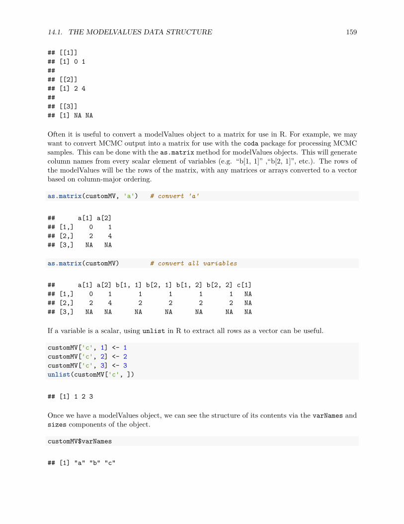
14.1. THE MODELVALUES DATA STRUCTURE 159
## [[1]]## [1] 0 1#### [[2]]## [1] 2 4#### [[3]]## [1] NA NA
Often it is useful to convert a modelValues object to a matrix for use in R. For example, we maywant to convert MCMC output into a matrix for use with the coda package for processing MCMCsamples. This can be done with the as.matrix method for modelValues objects. This will generatecolumn names from every scalar element of variables (e.g. “b[1, 1]” ,“b[2, 1]”, etc.). The rows ofthe modelValues will be the rows of the matrix, with any matrices or arrays converted to a vectorbased on column-major ordering.
as.matrix(customMV, 'a') # convert 'a'
## a[1] a[2]## [1,] 0 1## [2,] 2 4## [3,] NA NA
as.matrix(customMV) # convert all variables
## a[1] a[2] b[1, 1] b[2, 1] b[1, 2] b[2, 2] c[1]## [1,] 0 1 1 1 1 1 NA## [2,] 2 4 2 2 2 2 NA## [3,] NA NA NA NA NA NA NA
If a variable is a scalar, using unlist in R to extract all rows as a vector can be useful.
customMV['c', 1] <- 1customMV['c', 2] <- 2customMV['c', 3] <- 3unlist(customMV['c', ])
## [1] 1 2 3
Once we have a modelValues object, we can see the structure of its contents via the varNames andsizes components of the object.
customMV$varNames
## [1] "a" "b" "c"

160 CHAPTER 14. DATA STRUCTURES IN NIMBLE
customMV$sizes
## $a## [1] 2#### $b## [1] 2 2#### $c## [1] 1
As with most NIMBLE objects, modelValues are passed by reference, not by value. That means anymodifications of modelValues objects in either R functions or nimbleFunctions will persist outsideof the function. This allows for more efficient computation, as stored values are immediately sharedamong nimbleFunctions.
alter_a <- function(mv){mv['a',1][1] <- 1
}customMV['a', 1]
## [1] 0 1
alter_a(customMV)customMV['a',1]
## [1] 1 1
However, when you retrieve a variable from a modelValues object, the result is a standard R list,which is subsequently passed by value, as usual in R.
14.1.2.1 Automating calculation and simulation using modelValues
The nimbleFunctions simNodesMV, calcNodesMV, and getLogProbsMV can be used to operate ona model based on rows in a modelValues object. For example, simNodesMV will simulate in themodel multiple times and record each simulation in a row of its modelValues. calcNodesMV andgetLogProbsMV iterate over the rows of a modelValues, copy the nodes into the model, and thendo their job of calculating or collecting log probabilities (densities), respectively. Each of thesereturns a numeric vector with the summed log probabilities of the chosen nodes from each row.calcNodesMV will save the log probabilities back into the modelValues object if saveLP = TRUE, arun-time argument.
Here are some examples:
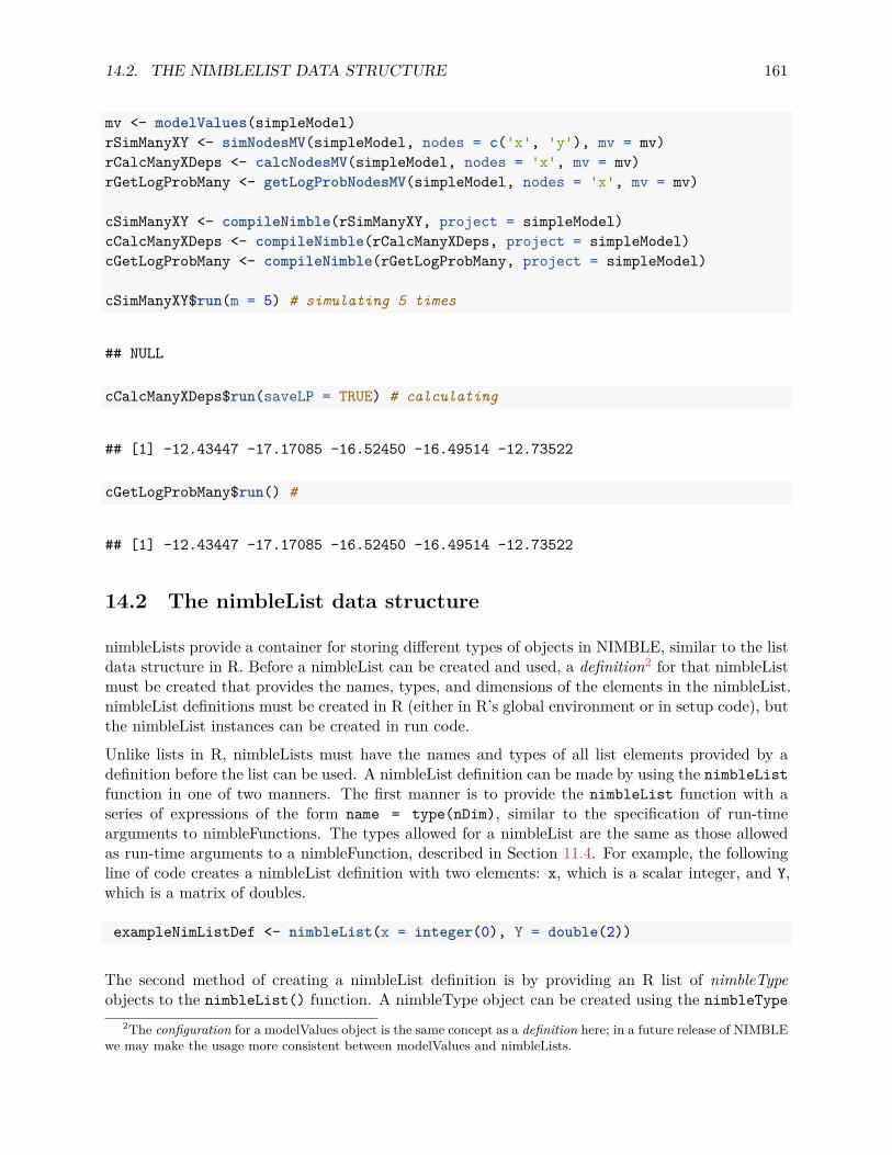
14.2. THE NIMBLELIST DATA STRUCTURE 161
mv <- modelValues(simpleModel)rSimManyXY <- simNodesMV(simpleModel, nodes = c('x', 'y'), mv = mv)rCalcManyXDeps <- calcNodesMV(simpleModel, nodes = 'x', mv = mv)rGetLogProbMany <- getLogProbNodesMV(simpleModel, nodes = 'x', mv = mv)
cSimManyXY <- compileNimble(rSimManyXY, project = simpleModel)cCalcManyXDeps <- compileNimble(rCalcManyXDeps, project = simpleModel)cGetLogProbMany <- compileNimble(rGetLogProbMany, project = simpleModel)
cSimManyXY$run(m = 5) # simulating 5 times
## NULL
cCalcManyXDeps$run(saveLP = TRUE) # calculating
## [1] -12.43447 -17.17085 -16.52450 -16.49514 -12.73522
cGetLogProbMany$run() #
## [1] -12.43447 -17.17085 -16.52450 -16.49514 -12.73522
14.2 The nimbleList data structure
nimbleLists provide a container for storing different types of objects in NIMBLE, similar to the listdata structure in R. Before a nimbleList can be created and used, a definition2 for that nimbleListmust be created that provides the names, types, and dimensions of the elements in the nimbleList.nimbleList definitions must be created in R (either in R’s global environment or in setup code), butthe nimbleList instances can be created in run code.
Unlike lists in R, nimbleLists must have the names and types of all list elements provided by adefinition before the list can be used. A nimbleList definition can be made by using the nimbleListfunction in one of two manners. The first manner is to provide the nimbleList function with aseries of expressions of the form name = type(nDim), similar to the specification of run-timearguments to nimbleFunctions. The types allowed for a nimbleList are the same as those allowedas run-time arguments to a nimbleFunction, described in Section 11.4. For example, the followingline of code creates a nimbleList definition with two elements: x, which is a scalar integer, and Y,which is a matrix of doubles.
exampleNimListDef <- nimbleList(x = integer(0), Y = double(2))
The second method of creating a nimbleList definition is by providing an R list of nimbleTypeobjects to the nimbleList() function. A nimbleType object can be created using the nimbleType
2The configuration for a modelValues object is the same concept as a definition here; in a future release of NIMBLEwe may make the usage more consistent between modelValues and nimbleLists.

162 CHAPTER 14. DATA STRUCTURES IN NIMBLE
function, which must be provided with three arguments: the name of the element being created,the type of the element being created, and the dim of the element being created. For example,the following code creates a list with two nimbleType objects and uses these objects to create animbleList definition.
nimbleListTypes <- list(nimbleType(name = 'x', type = 'integer', dim = 0),nimbleType(name = 'Y', type = 'double', dim = 2))
# this nimbleList definition is identical to the one created aboveexampleNimListDef2 <- nimbleList(nimbleListTypes)
Creating definitions using a list of nimbleTypes can be useful, as it allows for programmatic gener-ation of nimbleList elements.Once a nimbleList definition has been created, new instances of nimbleLists can be made from thatdefinition using the new member function. The new function can optionally take initial values forthe list elements as arguments. Below, we create a new nimbleList from our exampleNimListDefand specify values for the two elements of our list:
exampleNimList <- exampleNimListDef$new(x = 1, Y = diag(2))
Once created, nimbleList elements can be accessed using the $ operator, just as with lists in R. Forexample, the value of the x element of our exampleNimbleList can be set to 7 using
exampleNimList$x <- 7
nimbleList definitions can be created either in R’s global environment or in setup code of a nimble-Function. Once a nimbleList definition has been made, new instances of nimbleLists can be createdusing the new function in R’s global environment, in setup code, or in run code of a nimbleFunction.nimbleLists can also be passed as arguments to run code of nimbleFunctions and returned fromnimbleFunctions. To use a nimbleList as a run function argument, the name of the nimbleListdefinition should be provided as the argument type, with a set of parentheses following. To returna nimbleList from the run code of a nimbleFunction, the returnType of that function should bethe name of the nimbleList definition, again using a following set of parentheses.Below, we demonstrate a function that takes the exampleNimList as an argument, modifies its Yelement, and returns the nimbleList.
mynf <- nimbleFunction(run = function(vals = exampleNimListDef()){
onesMatrix <- matrix(value = 1, nrow = 2, ncol = 2)vals$Y <- onesMatrixreturnType(exampleNimListDef())return(vals)
})
# pass exampleNimList as argument to mynfmynf(exampleNimList)

14.2. THE NIMBLELIST DATA STRUCTURE 163
## nimbleList object of type nfRefClass_63## Field "x":## [1] 7## Field "Y":## [,1] [,2]## [1,] 1 1## [2,] 1 1
nimbleList arguments to run functions are passed by reference – this means that if an elementof a nimbleList argument is modified within a function, that element will remain modified whenthe function has finished running. To see this, we can inspect the value of the Y element of theexampleNimList object and see that it has been modified.
exampleNimList$Y
## [,1] [,2]## [1,] 1 1## [2,] 1 1
In addition to storing basic data types, nimbleLists can also store other nimbleLists. To achieve this,we must create a nimbleList definition that declares the types of nested nimbleLists a nimbleListwill store. Below, we create two types of nimbleLists: the first, named innerNimList, will be storedinside the second, named outerNimList:
# first, create definitions for both inner and outer nimbleListsinnerNimListDef <- nimbleList(someText = character(0))outerNimListDef <- nimbleList(xList = innerNimListDef(),
z = double(0))
# then, create outer nimbleListouterNimList <- outerNimListDef$new(z = 3.14)
# access element of inner nimbleListouterNimList$xList$someText <- "hello, world"
Note that definitions for inner, or nested, nimbleLists must be created before the definition for anouter nimbleList.
14.2.1 Using eigen and svd in nimbleFunctions
NIMBLE has two linear algebra functions that return nimbleLists. The eigen function takes a sym-metic matrix, x, as an argument and returns a nimbleList of type eigenNimbleList. nimbleLists oftype eigenNimbleList have two elements: values, a vector with the eigenvalues of x, and vectors,a square matrix with the same dimension as x whose columns are the eigenvectors of x. The eigenfunction has two additional arguments: symmetric and only.values. The symmetric argumentcan be used to specify if x is a symmetric matrix or not. If symmetric = FALSE (the default value),
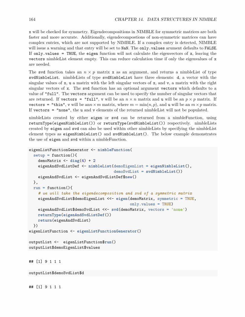
164 CHAPTER 14. DATA STRUCTURES IN NIMBLE
x will be checked for symmetry. Eigendecompositions in NIMBLE for symmetric matrices are bothfaster and more accurate. Additionally, eigendecompostions of non-symmetric matrices can havecomplex entries, which are not supported by NIMBLE. If a complex entry is detected, NIMBLEwill issue a warning and that entry will be set to NaN. The only.values arument defaults to FALSE.If only.values = TRUE, the eigen function will not calculate the eigenvectors of x, leaving thevectors nimbleList element empty. This can reduce calculation time if only the eigenvalues of xare needed.The svd function takes an n × p matrix x as an argument, and returns a nimbleList of typesvdNimbleList. nimbleLists of type svdNimbleList have three elements: d, a vector with thesingular values of x, u a matrix with the left singular vectors of x, and v, a matrix with the rightsingular vectors of x. The svd function has an optional argument vectors which defaults to avalue of "full". The vectors argument can be used to specify the number of singular vectors thatare returned. If vectors = "full", v will be an n × n matrix and u will be an p × p matrix. Ifvectors = "thin", v will be ann × m matrix, where m = min(n, p), and u will be an m × p matrix.If vectors = "none", the u and v elements of the returned nimbleList will not be populated.nimbleLists created by either eigen or svd can be returned from a nimbleFunction, usingreturnType(eigenNimbleList()) or returnType(svdNimbleList()) respectively. nimbleListscreated by eigen and svd can also be used within other nimbleLists by specifying the nimbleListelement types as eigenNimbleList() and svdNimbleList(). The below example demonstratesthe use of eigen and svd within a nimbleFunction.
eigenListFunctionGenerator <- nimbleFunction(setup = function(){
demoMatrix <- diag(4) + 2eigenAndSvdListDef <- nimbleList(demoEigenList = eigenNimbleList(),
demoSvdList = svdNimbleList())eigenAndSvdList <- eigenAndSvdListDef$new()
},run = function(){
# we will take the eigendecomposition and svd of a symmetric matrixeigenAndSvdList$demoEigenList <<- eigen(demoMatrix, symmetric = TRUE,
only.values = TRUE)eigenAndSvdList$demoSvdList <<- svd(demoMatrix, vectors = 'none')returnType(eigenAndSvdListDef())return(eigenAndSvdList)
})eigenListFunction <- eigenListFunctionGenerator()
outputList <- eigenListFunction$run()outputList$demoEigenList$values
## [1] 9 1 1 1
outputList$demoSvdList$d
## [1] 9 1 1 1

14.2. THE NIMBLELIST DATA STRUCTURE 165
The eigenvalues and singular values returned from the above function are the same since the matrixbeing decomposed was symmetric. However, note that both eigendecompositions and singular valuedecompositions are numerical procedures, and computed solutions may have slight differences evenfor a symmetric input matrix.

166 CHAPTER 14. DATA STRUCTURES IN NIMBLE

Chapter 15
Writing nimbleFunctions to interactwith models
15.1 Overview
When you write an R function, you say what the input arguments are, you provide the code forexecution, and in that code you give the value to be returned1. Using the function keyword in Rtriggers the operation of creating an object that is the function.
Creating nimbleFunctions is similar, but there are two kinds of code and two steps of execution:
1. Setup code is provided as a regular R function, but the programmer does not control whatit returns. Typically the inputs to setup code are objects like a model, a vector of nodes, amodelValues object or a modelValues configuration, or another nimbleFunction. The setupcode, as its name implies, sets up information for run-time code. It is executed in R, so itcan use any aspect of R.
2. Run code is provided in the NIMBLE language, which was introduced in Chapter 11. This issimilar to a narrow subset of R, but it is important to remember that it is different – definedby what can be compiled – and much more limited. Run code can use the objects created bythe setup code. In addition, some information on variable types must be provided for inputarguments, the return value, and in some circumstances for local variables. There are twokinds of run code:
a. There is always a primary function, given as the argument run2.b. There can optionally be other functions, or ‘methods’ in the language of object-oriented
programming, that share the same objects created by the setup function.
Here is a small example to fix ideas:
1Normally this is the value of the last evaluated code, or the argument to return.2This can be omitted if you don’t need it.
167

168 CHAPTER 15. WRITING NIMBLEFUNCTIONS TO INTERACT WITH MODELS
logProbCalcPlus <- nimbleFunction(setup = function(model, node) {
dependentNodes <- model$getDependencies(node)valueToAdd <- 1
},run = function(P = double(0)) {
model[[node]] <<- P + valueToAddreturn(model$calculate(dependentNodes))returnType(double(0))
})
code <- nimbleCode({a ~ dnorm(0, 1)b ~ dnorm(a, 1)
})testModel <- nimbleModel(code, check = FALSE)logProbCalcPlusA <- logProbCalcPlus(testModel, "a")testModel$b <- 1.5logProbCalcPlusA$run(0.25)
## [1] -2.650377
dnorm(1.25,0,1,TRUE)+dnorm(1.5,1.25,1,TRUE) # direct validation
## [1] -2.650377
testModel$a # "a" was set to 0.5 + valueToAdd
## [1] 1.25
The call to the R function called nimbleFunction returns a function, similarly to defining a func-tion in R. That function, logProbCalcPlus, takes arguments for its setup function, executes it,and returns an object, logProbCalcPlusA, that has a run member function (method) accessedby $run. In this case, the setup function obtains the stochastic dependencies of the node us-ing the getDependencies member function of the model (see Section 13.1.3) and stores them independentNodes. In this way, logProbCalcPlus can adapt to any model. It also creates a variable,valueToAdd, that can be used by the nimbleFunction.
The object logProbCalcPlusA, returned by logProbCalcPlus, is permanently bound to the resultsof the processed setup function. In this case, logProbCalcPlusA$run takes a scalar input value,P, assigns P + valueToAdd to the given node in the model, and returns the sum of the log proba-bilities of that node and its stochastic dependencies3. We say logProbCalcPlusA is an ‘instance’
3Note the use of the global assignment operator to assign into the model. This is necessary for assigning intovariables from the setup function, at least if you want to avoid warnings from R. These warnings come from R’sreference class system.

15.2. USING AND COMPILING NIMBLEFUNCTIONS 169
of logProbCalcPlus that is ‘specialized’ or ‘bound’ to a and testModel. Usually, the setup codewill be where information about the model structure is determined, and then the run code can usethat information without repeatedly, redundantly recomputing it. A nimbleFunction can be calledrepeatedly (one can think of it as a generator), each time returning a specialized nimbleFunction.
Readers familiar with object-oriented programming may find it useful to think in terms of classdefinitions and objects. nimbleFunction creates a class definition. Each specialized nimbleFunctionis one object in the class. The setup arguments are used to define member data in the object.
15.2 Using and compiling nimbleFunctions
To compile the nimbleFunction, together with its model, we use compileNimble:
CnfDemo <- compileNimble(testModel, logProbCalcPlusA)CtestModel <- CnfDemo$testModelClogProbCalcPlusA <- CnfDemo$logProbCalcPlusA
These have been initialized with the values from their uncompiled versions and can be used in thesame way:
CtestModel$a # values were initialized from testModel
## [1] 1.25
CtestModel$b
## [1] 1.5
lpA <- ClogProbCalcPlusA$run(1.5)lpA
## [1] -5.462877
# verify the answer:dnorm(CtestModel$b, CtestModel$a, 1, log = TRUE) +
dnorm(CtestModel$a, 0, 1, log = TRUE)
## [1] -5.462877
CtestModel$a # a was modified in the compiled model
## [1] 2.5

170 CHAPTER 15. WRITING NIMBLEFUNCTIONS TO INTERACT WITH MODELS
testModel$a # the uncompiled model was not modified
## [1] 1.25
15.3 Writing setup code
15.3.1 Useful tools for setup functions
The setup function is typically used to determine information on nodes in a model, set up model-Values or nimbleList objects, set up (nested) nimbleFunctions or nimbleFunctionLists, and set upany persistent numeric objects. For example, the setup code of an MCMC nimbleFunction createsthe nimbleFunctionList of sampler nimbleFunctions. The values of numeric objects created in setupcode can be modified by run code and will persist across calls.
Some of the useful tools and objects to create in setup functions include:
• vectors of node names, often from a model Often these are obtained from thegetNodeNames, getDependencies, and other methods of a model, described in Sections13.1-13.2.
• modelValues objects These are discussed in Sections 14.1 and 15.4.4.• nimbleList objects New instances of nimbleLists can be created from a nimbleList defini-
tion in either setup or run code. See Section 14.2 for more information.• specializations of other nimbleFunctions A useful NIMBLE programming technique is
to have one nimbleFunction contain other nimbleFunctions, which it can use in its run-timecode (Section 15.4.7).
• lists of other nimbleFunctions In addition to containing single other nimbleFunctions, animbleFunction can contain a list of other nimbleFunctions (Section 15.4.8).
If one wants a nimbleFunction that does get specialized but has empty setup code, use setup =function() {} or setup = TRUE.
15.3.2 Accessing and modifying numeric values from setup
While models and nodes created during setup cannot be modified4, numeric values and modelValuescan be, as illustrated by extending the example from above.
logProbCalcPlusA$valueToAdd # in the uncompiled version
## [1] 1
logProbCalcPlusA$valueToAdd <- 2ClogProbCalcPlusA$valueToAdd # or in the compiled version
4Actually, they can be, but only for uncompiled nimbleFunctions.

15.4. WRITING RUN CODE 171
## [1] 1
ClogProbCalcPlusA$valueToAdd <- 3ClogProbCalcPlusA$run(1.5)
## [1] -16.46288
CtestModel$a # a == 1.5 + 3
## [1] 4.5
15.3.3 Determining numeric types in nimbleFunctions
For numeric variables from the setup function that appear in the run function or other memberfunctions (or are declared in setupOutputs), the type is determined from the values created bythe setup code. The types created by setup code must be consistent across all specializationsof the nimbleFunction. For example if X is created as a matrix (two-dimensional double) in onespecialization but as a vector (one-dimensional double) in another, there will be a problem duringcompilation. The sizes may differ in each specialization.
Treatment of vectors of length one presents special challenges because they could be treated asscalars or vectors. Currently they are treated as scalars. If you want a vector, ensure that thelength is greater than one in the setup code and then use setSize in the run-time code.
15.3.4 Control of setup outputs
Sometimes setup code may create variables that are not used in run code. By default, NIMBLEinspects run code and omits variables from setup that do not appear in run code from compila-tion. However, sometimes a programmer may want to force a numeric or character variable to beincluded in compilation, even if it is not used directly in run code. As shown below, such variablescan be directly accessed in one nimbleFunction from another, which provides a way of using nim-bleFunctions as general data structures. To force NIMBLE to include variables during compilation,for example X and Y, simply include
setupOutputs(X, Y)
anywhere in the setup code.
15.4 Writing run code
In Chapter 11 we described the functionality of the NIMBLE language that could be used in runcode without setup code (typically in cases where no models or modelValues are needed). Next weexplain the additional features that allow use of models and modelValues in the run code.

172 CHAPTER 15. WRITING NIMBLEFUNCTIONS TO INTERACT WITH MODELS
15.4.1 Driving models: calculate, calculateDiff, simulate, getLogProb
These four functions are the primary ways to operate a model. Their syntax was explained inSection 13.3. Except for getLogProb, it is usually important for the nodes vector to be sorted intopological order. Model member functions such as getDependencies and expandNodeNames willalways return topoligically sorted node names.
Most R-like indexing of a node vector is allowed within the argument to calculate, calculateDiff,simulate, and getLogProb. For example, all of the following are allowed:
myModel$calculate(nodes)myModel$calculate(nodes[i])myModel$calculate(nodes[1:3])myModel$calculate(nodes[c(1,3)])myModel$calculate(nodes[2:i])myModel$calculate(nodes[ values(model, nodes) + 0.1 < x ])
Note that one cannot create new vectors of nodes in run code. They can only be indexed within acall to calculate, calculateDiff, simulate or getLogProb.
15.4.2 Getting and setting variable and node values
15.4.2.1 Using indexing with nodes
Here is an example that illustrates getting and setting of nodes, subsets of nodes, or variables. Notethe following:
• In model[[v]], v can only be a single node or variable name, not a vector of multiple nodesnor an element of such a vector (model[[ nodes[i] ]] does not work). The node itself maybe a vector, matrix or array node.
• In fact, v can be a node-name-like character string, even if it is not actually a node in themodel. See example 4 in the code below.
• One can also use model$varName, with the caveat that varName must be a variable name.This usage would only make sense for a nimbleFunction written for models known to havea specific variable. (Note that if a is a scalar node in model, then model[['a']] will be ascalar but model$a will be a vector of length -)
• one should use the <<- global assignment operator to assign into model nodes.
Note that NIMBLE does not allow variables to change dimensions. Model nodes are the same, andindeed are more restricted because they can’t change sizes. In addition, NIMBLE distinguishesbetween scalars and vectors of length 1. These rules, and ways to handle them correctly, areillustrated in the following code as well as in Section 11.3.
code <- nimbleCode({z ~ dnorm(0, sd = sigma)sigma ~ dunif(0, 10)y[1:n] ~ dmnorm(zeroes[1:n], cov = C[1:5, 1:5])
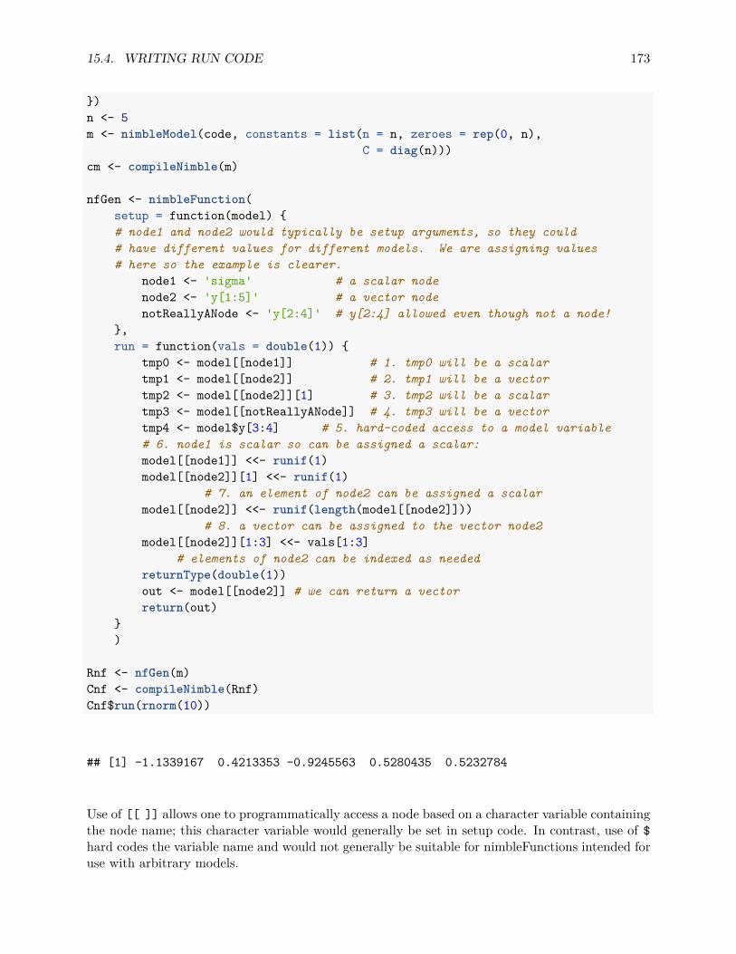
15.4. WRITING RUN CODE 173
})n <- 5m <- nimbleModel(code, constants = list(n = n, zeroes = rep(0, n),
C = diag(n)))cm <- compileNimble(m)
nfGen <- nimbleFunction(setup = function(model) {# node1 and node2 would typically be setup arguments, so they could# have different values for different models. We are assigning values# here so the example is clearer.
node1 <- 'sigma' # a scalar nodenode2 <- 'y[1:5]' # a vector nodenotReallyANode <- 'y[2:4]' # y[2:4] allowed even though not a node!
},run = function(vals = double(1)) {
tmp0 <- model[[node1]] # 1. tmp0 will be a scalartmp1 <- model[[node2]] # 2. tmp1 will be a vectortmp2 <- model[[node2]][1] # 3. tmp2 will be a scalartmp3 <- model[[notReallyANode]] # 4. tmp3 will be a vectortmp4 <- model$y[3:4] # 5. hard-coded access to a model variable# 6. node1 is scalar so can be assigned a scalar:model[[node1]] <<- runif(1)model[[node2]][1] <<- runif(1)
# 7. an element of node2 can be assigned a scalarmodel[[node2]] <<- runif(length(model[[node2]]))
# 8. a vector can be assigned to the vector node2model[[node2]][1:3] <<- vals[1:3]
# elements of node2 can be indexed as neededreturnType(double(1))out <- model[[node2]] # we can return a vectorreturn(out)
})
Rnf <- nfGen(m)Cnf <- compileNimble(Rnf)Cnf$run(rnorm(10))
## [1] -1.1339167 0.4213353 -0.9245563 0.5280435 0.5232784
Use of [[ ]] allows one to programmatically access a node based on a character variable containingthe node name; this character variable would generally be set in setup code. In contrast, use of $hard codes the variable name and would not generally be suitable for nimbleFunctions intended foruse with arbitrary models.

174 CHAPTER 15. WRITING NIMBLEFUNCTIONS TO INTERACT WITH MODELS
15.4.2.2 Getting and setting more than one model node or variable at a time usingvalues
Sometimes it is useful to set a collection of nodes or variables at one time. For example, one mightwant a nimbleFunction that will serve as the objective function for an optimizer. The input to thenimbleFunction would be a vector, which should be used to fill a collection of nodes in the modelbefore calculating their log probabilities. This can be done using values:
# get values from a set of model nodes into a vectorP <- values(model, nodes)# or put values from a vector into a set of model nodesvalues(model, nodes) <- P
where the first line would assign the collection of values from nodes into P, and the second woulddo the inverse. In both cases, values from nodes with two or more dimensions are flattened into avector in column-wise order.
values(model, nodes) may be used as a vector in other expressions, e.g.,
Y <- A %*% values(model, nodes) + b
One can also index elements of nodes in the argument to values, in the same manner as discussedfor calculate and related functions in Section 15.4.1.
Note again the potential for confusion between scalars and vectors of length 1. values returns avector and expects a vector when used on the left-hand side of an assignment. If only a single valueis being assigned, it must be a vector of length 1, not a scalar. This can be achieved by wrappinga scalar in c() when necessary. For example:
# c(rnorm(1)) creates vector of length one:values(model, nodes[1]) <- c(rnorm(1))# won't compile because rnorm(1) is a scalar# values(model, nodes[1]) <- rnorm(1)
out <- values(model, nodes[1]) # out is a vectorout2 <- values(model, nodes[1])[1] # out2 is a scalar
15.4.3 Getting parameter values and node bounds
Sections 13.2.3-13.2.4 describe how to get the parameter values for a node and the range (bounds)of possible values for the node using getParam and getBound. Both of these can be used in runcode.
15.4.4 Using modelValues objects
The modelValues structure was introduced in Section 14.1. Inside nimbleFunctions, modelValuesare designed to easily save values from a model object during the running of a nimbleFunction. A

15.4. WRITING RUN CODE 175
modelValues object used in run code must always exist in the setup code, either by passing it in asa setup argument or creating it in the setup code.
To illustrate this, we will create a nimbleFunction for computing importance weights for impor-tance sampling. This function will use two modelValues objects. propModelValues will containa set of values simulated from the importance sampling distribution and a field propLL for theirlog probabilities (densities). savedWeights will contain the difference in log probability (density)between the model and the propLL value provided for each set of values.
# Accepting modelValues as a setup argumentswConf <- modelValuesConf(vars = "w",
types = "double",sizes = 1)
setup = function(propModelValues, model, savedWeightsConf){# Building a modelValues in the setup functionsavedWeights <- modelValues(conf = savedWeightsConf)# List of nodes to be used in run functionmodelNodes <- model$getNodeNames(stochOnly = TRUE,
includeData = FALSE)}
The simplest way to pass values back and forth between models and modelValues inside of animbleFunction is with copy, which has the synonym nimCopy. See help(nimCopy) for argumentdetails.
Alternatively, the values may be accessed via indexing of individual rows, using the notationmv[var, i], where mv is a modelValues object, var is a variable name (not a node name), and iis a row number. Likewise, the getsize and resize functions can be used as discussed in Section14.1. However the function as.matrix does not work in run code.
Here is a run function to use these modelValues:
run = function(){# gets the number of rows of propSamplesm <- getsize(propModelValues)
# resized savedWeights to have the proper rowsresize(savedWeights, m)for(i in 1:m){
# Copying from propSamples to model.# Node names of propSamples and model must match!nimCopy(from = propModelValues, to = model, row = i,
nodes = modelNodes, logProb = FALSE)# calculates the log likelihood of the modeltargLL <- model$calculate()# retreaves the saved log likelihood from the proposed modelpropLL <- propModelValues["propLL",i][1]# saves the importance weight for the i-th samplesavedWeights["w", i][1] <<- exp(targLL - propLL)
176 CHAPTER 15. WRITING NIMBLEFUNCTIONS TO INTERACT WITH MODELS
}# does not return anything
}
Once the nimbleFunction is built, the modelValues object can be accessed using $, which is shownin more detail below. In fact, since modelValues, like most NIMBLE objects, are reference classobjects, one can get a reference to them before the function is executed and then use that referenceafterwards.
# simple model and modelValues for example use with code abovetargetModelCode <- nimbleCode({
x ~ dnorm(0,1)for(i in 1:4)
y[i] ~ dnorm(0,1)})
# code for proposal modelpropModelCode <- nimbleCode({
x ~ dnorm(0,2)for(i in 1:4)
y[i] ~ dnorm(0,2)})
# creating the modelstargetModel = nimbleModel(targetModelCode, check = FALSE)propModel = nimbleModel(propModelCode, check = FALSE)cTargetModel = compileNimble(targetModel)cPropModel = compileNimble(propModel)
sampleMVConf = modelValuesConf(vars = c("x", "y", "propLL"),types = c("double", "double", "double"),sizes = list(x = 1, y = 4, propLL = 1) )
sampleMV <- modelValues(sampleMVConf)
# nimbleFunction for generating proposal samplePropSamp_Gen <- nimbleFunction(
setup = function(mv, propModel){nodeNames <- propModel$getNodeNames()
},run = function(m = integer() ){
resize(mv, m)for(i in 1:m){
propModel$simulate()nimCopy(from = propModel, to = mv, nodes = nodeNames, row = i)mv["propLL", i][1] <<- propModel$calculate()

15.4. WRITING RUN CODE 177
}})
# nimbleFunction for calculating importance weights# uses setup and run functions as defined in previous code chunkimpWeights_Gen <- nimbleFunction(setup = setup,
run = run)
# making instances of nimbleFunctions# note that both functions share the same modelValues objectRPropSamp <- PropSamp_Gen(sampleMV, propModel)RImpWeights <- impWeights_Gen(sampleMV, targetModel, swConf)
# compilingCPropSamp <- compileNimble(RPropSamp, project = propModel)CImpWeights <- compileNimble(RImpWeights, project = targetModel)
# generating and saving proposal sample of size 10CPropSamp$run(10)
## NULL
# calculating the importance weights and saving to mvCImpWeights$run()
## NULL
# retrieving the modelValues objects# extracted objects are C-based modelValues objects
savedPropSamp_1 = CImpWeights$propModelValuessavedPropSamp_2 = CPropSamp$mv
# Subtle note: savedPropSamp_1 and savedPropSamp_2# both provide interface to the same compiled modelValues objects!# This is because they were both built from sampleMV.
savedPropSamp_1["x",1]
## [1] 0.5615461

178 CHAPTER 15. WRITING NIMBLEFUNCTIONS TO INTERACT WITH MODELS
savedPropSamp_2["x",1]
## [1] 0.5615461
savedPropSamp_1["x",1] <- 0 # example of directly setting a valuesavedPropSamp_2["x",1]
## [1] 0
# viewing the saved importance weightssavedWeights <- CImpWeights$savedWeightsunlist(savedWeights[["w"]])
## [1] 0.3159913 0.3114850 1.3655582 0.3969088 41.3934032 0.2732388## [7] 0.7972150 1.5456142 0.4199902 1.8547728
# viewing first 3 rows -- note that savedPropSsamp_1["x", 1] was alteredas.matrix(savedPropSamp_1)[1:3, ]
## propLL[1] x[1] y[1] y[2] y[3] y[4]## [1,] -4.023479 0.0000000 -0.4634227 -0.4790402 0.1299793 0.6206335## [2,] -3.994752 -0.2773491 -0.4730179 -0.7142721 -0.5309174 -0.2005022## [3,] -6.950687 -0.8243472 0.4887699 -1.4541917 -0.1090178 -1.0216946
Importance sampling could also be written using simple vectors for the weights, but we illustratedputting them in a modelValues object along with model variables.
15.4.5 Using model variables and modelValues in expressions
Each way of accessing a variable, node, or modelValues can be used amidst mathematical expres-sions, including with indexing, or passed to another nimbleFunction as an argument. For example,the following two statements would be valid:
model[["x[2:8, ]"]][2:4, 1:3] %*% Z
if Z is a vector or matrix, and
C[6:10] <- mv[v, i][1:5, k] + B
if B is a vector or matrix.The NIMBLE language allows scalars, but models defined from BUGS code are never created aspurely scalar nodes. Instead, a single node such as defined by z ~ dnorm(0, 1) is implemented asa vector of length 1, similar to R. When using z via model$z or model[["z"]], NIMBLE will tryto do the right thing by treating this as a scalar. In the event of problems5, a more explicit way toaccess z is model$z[1] or model[["z"]][1].
5Please tell us!

15.4. WRITING RUN CODE 179
15.4.6 Including other methods in a nimbleFunction
Other methods can be included with the methods argument to nimbleFunction. These methodscan use the objects created in setup code in just the same ways as the run function. In fact, therun function is just a default main method name. Any method can then call another method.
methodsDemo <- nimbleFunction(setup = function() {sharedValue <- 1},run = function(x = double(1)) {
print("sharedValues = ", sharedValue, "\n")increment()print("sharedValues = ", sharedValue, "\n")A <- times(5)return(A * x)returnType(double(1))
},methods = list(
increment = function() {sharedValue <<- sharedValue + 1
},times = function(factor = double()) {
return(factor * sharedValue)returnType(double())
}))
methodsDemo1 <- methodsDemo()methodsDemo1$run(1:10)
## sharedValues = 1#### sharedValues = 2
## [1] 10 20 30 40 50 60 70 80 90 100
methodsDemo1$sharedValue <- 1CmethodsDemo1 <- compileNimble(methodsDemo1)CmethodsDemo1$run(1:10)
## sharedValues = 1#### sharedValues = 2
## [1] 10 20 30 40 50 60 70 80 90 100

180 CHAPTER 15. WRITING NIMBLEFUNCTIONS TO INTERACT WITH MODELS
15.4.7 Using other nimbleFunctions
One nimbleFunction can use another nimbleFunction that was passed to it as a setup argument orwas created in the setup function. This can be an effective way to program. When a nimbleFunctionneeds to access a setup variable or method of another nimbleFunction, use $.
usePreviousDemo <- nimbleFunction(setup = function(initialSharedValue) {
myMethodsDemo <- methodsDemo()},run = function(x = double(1)) {
myMethodsDemo$sharedValue <<- initialSharedValueprint(myMethodsDemo$sharedValue)A <- myMethodsDemo$run(x[1:5])print(A)B <- myMethodsDemo$times(10)return(B)returnType(double())
})
usePreviousDemo1 <- usePreviousDemo(2)usePreviousDemo1$run(1:10)
## 2## sharedValues = 2#### sharedValues = 3#### 15 30 45 60 75
## [1] 30
CusePreviousDemo1 <- compileNimble(usePreviousDemo1)CusePreviousDemo1$run(1:10)
## 2## sharedValues = 2#### sharedValues = 3#### 15## 30## 45## 60## 75
## [1] 30

15.4. WRITING RUN CODE 181
15.4.8 Virtual nimbleFunctions and nimbleFunctionLists
Often it is useful for one nimbleFunction to have a list of other nimbleFunctions, all of whosemethods have the same arguments and return types. For example, NIMBLE’s MCMC enginecontains a list of samplers that are each nimbleFunctions.
To make such a list, NIMBLE provides a way to declare the arguments and return types of methods:virtual nimbleFunctions created by nimbleFunctionVirtual. Other nimbleFunctions can inheritfrom virtual nimbleFunctions, which in R is called ‘containing’ them. Readers familiar with objectoriented programming will recognize this as a simple class inheritance system. In Version 0.6-12 itis limited to simple, single-level inheritance.
Here is how it works:
baseClass <- nimbleFunctionVirtual(run = function(x = double(1)) {returnType(double())},methods = list(
foo = function() {returnType(double())}))
derived1 <- nimbleFunction(contains = baseClass,setup = function(){},run = function(x = double(1)) {
print("run 1")return(sum(x))returnType(double())
},methods = list(
foo = function() {print("foo 1")return(rnorm(1, 0, 1))returnType(double())
}))
derived2 <- nimbleFunction(contains = baseClass,setup = function(){},run = function(x = double(1)) {
print("run 2")return(prod(x))returnType(double())
},methods = list(
foo = function() {print("foo 2")return(runif(1, 100, 200))returnType(double())
}))

182 CHAPTER 15. WRITING NIMBLEFUNCTIONS TO INTERACT WITH MODELS
useThem <- nimbleFunction(setup = function() {
nfl <- nimbleFunctionList(baseClass)nfl[[1]] <- derived1()nfl[[2]] <- derived2()
},run = function(x = double(1)) {
for(i in seq_along(nfl)) {print( nfl[[i]]$run(x) )print( nfl[[i]]$foo() )
}})
useThem1 <- useThem()set.seed(1)useThem1$run(1:5)
## run 1## 15## foo 1## -0.6264538## run 2## 120## foo 2## 157.2853
CuseThem1 <- compileNimble(useThem1)set.seed(1)CuseThem1$run(1:5)
## run 1## 15## foo 1## -0.626454## run 2## 120## foo 2## 157.285
## NULL
One can also use seq_along with nimbleFunctionLists (and only with nimbleFunctionLists). Asin R, seq_along(myFunList) is equivalent to 1:length(myFunList) if the length of myFunList isgreater than zero. It is an empty sequence if the length is zero.Virtual nimbleFunctions cannot define setup values to be inherited.
15.4. WRITING RUN CODE 183
15.4.9 Character objects
NIMBLE provides limited uses of character objects in run code. Character vectors created in setupcode will be available in run code, but the only thing you can really do with them is include themin a print or stop statement.
Note that character vectors of model node and variable names are processed during compilation. Forexample, in model[[node]], node may be a character object, and the NIMBLE compiler processesthis differently than print("The node name was ", node). In the former, the NIMBLE compilersets up a C++ pointer directly to the node in the model, so that the character content of node isnever needed in C++. In the latter, node is used as a C++ string and therefore is needed in C++.
15.4.10 User-defined data structures
Before the introduction of nimbleLists in Version 0.6-4, NIMBLE did not explicitly have user-defineddata structures. An alternative way to create a data structure in NIMBLE is to use nimbleFunctionsto achieve a similar effect. To do so, one can define setup code with whatever variables are wantedand ensure they are compiled using setupOutputs. Here is an example:
dataNF <- nimbleFunction(setup = function() {
X <- 1Y <- as.numeric(c(1, 2))Z <- matrix(as.numeric(1:4), nrow = 2)setupOutputs(X, Y, Z)
})
useDataNF <- nimbleFunction(setup = function(myDataNF) {},run = function(newX = double(), newY = double(1), newZ = double(2)) {
myDataNF$X <<- newXmyDataNF$Y <<- newYmyDataNF$Z <<- newZ
})
myDataNF <- dataNF()myUseDataNF <- useDataNF(myDataNF)myUseDataNF$run(as.numeric(100), as.numeric(100:110),
matrix(as.numeric(101:120), nrow = 2))myDataNF$X
## [1] 100
myDataNF$Y
## [1] 100 101 102 103 104 105 106 107 108 109 110
184 CHAPTER 15. WRITING NIMBLEFUNCTIONS TO INTERACT WITH MODELS
myDataNF$Z
## [,1] [,2] [,3] [,4] [,5] [,6] [,7] [,8] [,9] [,10]## [1,] 101 103 105 107 109 111 113 115 117 119## [2,] 102 104 106 108 110 112 114 116 118 120
myUseDataNF$myDataNF$X
## [1] 100
nimbleOptions(buildInterfacesForCompiledNestedNimbleFunctions = TRUE)CmyUseDataNF <- compileNimble(myUseDataNF)CmyUseDataNF$run(-100, -(100:110), matrix(-(101:120), nrow = 2))
## NULL
CmyDataNF <- CmyUseDataNF$myDataNFCmyDataNF$X
## [1] -100
CmyDataNF$Y
## [1] -100 -101 -102 -103 -104 -105 -106 -107 -108 -109 -110
CmyDataNF$Z
## [,1] [,2] [,3] [,4] [,5] [,6] [,7] [,8] [,9] [,10]## [1,] -101 -103 -105 -107 -109 -111 -113 -115 -117 -119## [2,] -102 -104 -106 -108 -110 -112 -114 -116 -118 -120
You’ll notice that:
• After execution of the compiled function, access to the X, Y, and Z is the same as forthe uncompiled case. This occurs because CmyUseDataNF is an interface to the compiledversion of myUseDataNF, and it provides access to member objects and functions. In thiscase, one member object is myDataNF, which is an interface to the compiled version ofmyUseDataNF$myDataNF, which in turn provides access to X, Y, and Z. To reduce memoryuse, NIMBLE defaults to not providing full interfaces to nested nimbleFunctions likemyUseDataNF$myDataNF. In this example we made it provide full interfaces by settingthe buildInterfacesForCompiledNestedNimbleFunctions option via nimbleOptions toTRUE. If we had left that option FALSE (its default value), we could still get to the valuesof interest using valueInCompiledNimbleFunction(CmyDataNF, 'X')
• We need to take care that at the time of compilation, the X, Y and Z values contain doublesvia as.numeric so that they are not compiled as integer objects.
• The myDataNF could be created in the setup code. We just provided it as a setup argumentto illustrate that option.

15.5. EXAMPLE: WRITING USER-DEFINED SAMPLERS TO EXTEND NIMBLE’S MCMC ENGINE185
15.5 Example: writing user-defined samplers to extend NIM-BLE’s MCMC engine
One important use of nimbleFunctions is to write additional samplers that can be used in NIMBLE’sMCMC engine. This allows a user to write a custom sampler for one or more nodes in a model, aswell as for programmers to provide general samplers for use in addition to the library of samplersprovided with NIMBLE.The following code illustrates how a NIMBLE developer would implement and use a Metropolis-Hastings random walk sampler with fixed proposal standard deviation.
my_RW <- nimbleFunction(
contains = sampler_BASE,
setup = function(model, mvSaved, target, control) {# proposal standard deviationscale <- if(!is.null(control$scale)) control$scale else 1calcNodes <- model$getDependencies(target)
},
run = function() {# initial model logProbmodel_lp_initial <- getLogProb(model, calcNodes)# generate proposalproposal <- rnorm(1, model[[target]], scale)# store proposal into modelmodel[[target]] <<- proposal# proposal model logProbmodel_lp_proposed <- calculate(model, calcNodes)
# log-Metropolis-Hastings ratiolog_MH_ratio <- model_lp_proposed - model_lp_initial
# Metropolis-Hastings step: determine whether or# not to accept the newly proposed valueu <- runif(1, 0, 1)if(u < exp(log_MH_ratio)) jump <- TRUEelse jump <- FALSE
# keep the model and mvSaved objects consistentif(jump) copy(from = model, to = mvSaved, row = 1,
nodes = calcNodes, logProb = TRUE)else copy(from = mvSaved, to = model, row = 1,
nodes = calcNodes, logProb = TRUE)},
methods = list( reset = function () {} )
186 CHAPTER 15. WRITING NIMBLEFUNCTIONS TO INTERACT WITH MODELS
)
The name of this sampler function, for the purposes of using it in anMCMC algorithm, is my_RW. Thus, this sampler can be added to an exisiting MCMC configurationobject conf using:
mcmcConf$addSampler(target = 'x', type = 'my_RW',control = list(scale = 0.1))
To be used within the MCMC engine, sampler functions definitions must adhere exactly to thefollowing:
• The nimbleFunction must include the contains statement contains = sampler_BASE.• The setup function must have the four arguments model, mvSaved, target, control, in
that order.• The run function must accept no arguments, and have no return value. Further, after execu-
tion it must leave the mvSaved modelValues object as an up-to-date copy of the values andlogProb values in the model object.
• The nimbleFunction must have a member method called reset, which takes no argumentsand has no return value.
The purpose of the setup function is generally two-fold. First, to extract control parameters fromthe control list; in the example, the proposal standard deviation scale. It is good practice tospecify default values for any control parameters that are not provided in the control argument,as done in the example. Second, to generate any sets of nodes needed in the run function. Inmany sampling algorithms, as here, calcNodes is used to represent the target node(s) and depen-dencies up to the first layer of stochastic nodes, as this is precisely what is required for calculatingthe Metropolis-Hastings acceptance probability. These probability calculations are done usingmodel$calculate(calcNodes).
In the run function, the mvSaved modelValues object is kept up-to-date with the current state ofthe model, depending on whether the proposed changed was accepted. This is done using the copyfunction, to copy values between the model and mvSaved objects.
15.6 Copying nimbleFunctions (and NIMBLE models)
NIMBLE relies heavily on R’s reference class system. When models, modelValues, and nimbleFunc-tions with setup code are created, NIMBLE generates a new, customized reference class definitionfor each. As a result, objects of these types are passed by reference and hence modified in placeby most NIMBLE operations. This is necessary to avoid a great deal of copying and returning andhaving to reassign large objects, both in processing models and nimbleFunctions and in runningalgorithms.
One cannot generally copy NIMBLE models or nimbleFunctions (specializations or generators)in a safe fashion, because of the references to other objects embedded within NIMBLE objects.However, the model member function newModel will create a new copy of the model from the

15.7. DEBUGGING NIMBLEFUNCTIONS 187
same model definition (Section 6.1.3). This new model can then be used with newly instantiatednimbleFunctions.
The reliable way to create new copies of nimbleFunctions is to re-run the R function callednimbleFunction and record the result in a new object. For example, say you have animbleFunction called foo and 1000 instances of foo are compiled as part of an algorithmrelated to a model called model1. If you then need to use foo in an algorithm for another model,model2, doing so may work without any problems. However, there are cases where the NIMBLEcompiler will tell you during compilation that the second set of foo instances cannot be builtfrom the previous compiled version. A solution is to re-define foo from the beginning – i.e. callnimbleFunction again – and then proceed with building and compiling the algorithm for model2.
15.7 Debugging nimbleFunctions
One of the main reasons that NIMBLE provides an R (uncompiled) version of each nimbleFunctionis for debugging. One can call debug on nimbleFunction methods (in particular the main runmethod, e.g., debug(mynf$run) and then step through the code in R using R’s debugger. One canalso insert browser calls into run code and then run the nimbleFunction from R.
In contrast, directly debugging a compiled nimbleFunction is difficult, although those familiarwith running R through a debugger and accessing the underlying C code may be able to operatesimilarly with NIMBLE code. We often resort to using print statements for debugging compiledcode. Expert users fluent in C++ may also try setting nimbleOptions(pauseAfterWritingFiles= TRUE) and adding debugging code into the generated C++ files.
15.8 Timing nimbleFunctions with run.time
If your nimbleFunctions are correct but slow to run, you can use benchmarking tools to look forbottlenecks and to compare different implementations. If your functions are very long-running (say1ms or more), then standard R benchmarking tools may suffice, e.g. the microbenchmark package
library(microbenchmark)microbenchmark(myCompiledFunVersion1(1.234),
myCompiledFunVersion2(1.234)) # Beware R <--> C++ overhead!
If your nimbleFunctions are very fast, say under 1ms, then microbenchmark will be inaccurate dueto R-to-C++ conversion overhead (that won’t happen in your actual functions). To get timinginformation in C++, NIMBLE provides a run.time function that avoids the R-to-C++ overhead.
myMicrobenchmark <- compileNimble(nimbleFunction(run = function(iters = integer(0)){
time1 <- run.time({for (t in 1:iters) myCompiledFunVersion1(1.234)
})time2 <- run.time({
for (t in 1:iters) myCompiledFunVersion2(1.234)
188 CHAPTER 15. WRITING NIMBLEFUNCTIONS TO INTERACT WITH MODELS
})return(c(time1, time2))returnType(double(1))
}))print(myMicroBenchmark(100000))
15.9 Reducing memory usage
NIMBLE can create a lot of objects in its processing, and some of them use R features such asreference classes that are heavy in memory usage. We have noticed that building large models canuse lots of memory. To help alleviate this, we provide two options, which can be controlled vianimbleOptions.
As noted above, the option buildInterfacesForCompiledNestedNimbleFunctions defaults toFALSE, which means NIMBLE will not build full interfaces to compiled nimbleFunctions that onyappear within other nimbleFunctions. If you want access to all such nimbleFunctions, use theoption buildInterfacesForCompiledNestedNimbleFunctions = TRUE.
The option clearNimbleFunctionsAfterCompiling is more drastic, and it is experimental, so‘buyer beware’. This will clear much of the contents of an uncompiled nimbleFunction object afterit has been compiled in an effort to free some memory. We expect to be able to keep makingNIMBLE more efficient – faster execution and lower memory use – in the future.

Bibliography
Andrieu, C., Doucet, A., and Holenstein, R. (2010). Particle Markov chain Monte Carlo methods.Journal of the Royal Statistical Society: Series B (Statistical Methodology), 72(3):269––342.
Banerjee, S., Carlin, B., and Gelfand, A. (2015). Hierarchical Modeling and Analysis for SpatialData. Chapman & Hall, Boca Raton, 2 edition.
Blackwell, D. and MacQueen, J. (1973). Ferguson distributions via Pólya urn schemes. The Annalsof Statistics, 1:353–355.
Escobar, M. D. (1994). Estimating normal means with a Dirichlet process prior. Journal of theAmerican Statistical Association, 89:268–277.
Escobar, M. D. and West, M. (1995). Bayesian density estimation and inference using mixtures.Journal of the American Statistical Association, 90:577–588.
Ferguson, T. S. (1973). A Bayesian analysis of some nonparametric problems. Annals of Statistics,1:209–230.
Ferguson, T. S. (1974). Prior distribution on the spaces of probability measures. Annals of Statistics,2:615–629.
George, E., Makov, U., and Smith, A. (1993). Conjugate likelihood distributions. ScandinavianJournal of Statistics, 20(2):147––156.
Ishwaran, H. and James, L. F. (2001). Gibbs sampling methods for stick-breaking priors. Journalof the American Statistical Association, 96(453):161–173.
Ishwaran, H. and James, L. F. (2002). Approximate Dirichlet process computing in finite normalmixtures: smoothing and prior information. Journal of Computational and Graphical Statistics,11:508–532.
Lo, A. Y. (1984). On a class of Bayesian nonparametric estimates I: Density estimates. The Annalsof Statistics, 12:351–357.
Lunn, D., Spiegelhalter, D., Thomas, A., and Best, N. (2009). The BUGS project: Evolution,critique and future directions. Statistics in Medicine, 28(25):3049––3067.
Neal, R. (2000). Markov chain sampling methods for Dirichlet process mixture models. Journal ofComputational and Graphical Statistics, 9:249–265.
Neal, R. M. (2003). Slice sampling. The Annals of Statistics, 31(3):705–741.
189

190 BIBLIOGRAPHY
Paciorek, C. (2009). Understanding intrinsic Gaussian Markov random field spatial models, in-cluding intrinsic conditional autoregressive models. Technical report, University of California,Berkeley.
Roberts, G. O. and Sahu, S. K. (1997). Updating schemes, correlation structure, blocking andparameterization for the Gibbs sampler. Journal of the Royal Statistical Society: Series B(Statistical Methodology), 59(2):291–317.
Rue, H. and Held, L. (2005). Gaussian Markov Random Fields: Theory and Applications. Chapman& Hall, Boca Raton.
Sethuraman, J. (1994). A constructive definition of Dirichlet prior. Statistica Sinica, 2:639–650.
Watanabe, S. (2010). Asymptotic equivalence of Bayes cross validation and widely applica-ble information criterion in singular learning theory. Journal of Machine Learning Research,11(Dec):3571–3594.


