Page 1
1
OULU BUSINESS SCHOOL
Niranjan Sapkota
EVALUATING PERFORMANCE CAPACITY OF HIGH FREQUENCY
TRADING STRATEGIES, BASED ON COMPARATIVE RATIOS AND
MARKET INEFFICIENCY AT HELSINKI STOCK EXCHANGE
Master’s Thesis
Department of Finance
November 2014
Page 2
2
ABSTRACT OF THE MASTER’S THESIS UNIVERSITY OF OULU
Oulu Business School
Unit: Department of Finance
Author: Niranjan Sapkota Supervisor: Kahra, Hannu, Professor
Title: EVALUATING PERFORMANCE CAPACITY OF HIGH FREQUENCY TRADING
STRATEGIES, BASED ON COMPARATIVE RATIOS AND MARKET INEFFICIENCY AT HELSINKI
STOCK EXCHANGE
Subject:
Finance
Type of the degree:
Master of Science (Economics and
Business Administration)
Time of publication:
November 2014
Number of pages:
77
Abstract:
High frequency trading is not only about the speed but also about the effective trading strategies it uses to
perform the trade. Performance capacity evaluation of high frequency trading strategies is done using
different comparative ratios. Studies find, due to tight spread, it is difficult for high frequency traders to
generate significant alpha by trading the highly liquid stocks using market making strategy. But they can
still generate positive return with Sharpe ratio almost equal to market. They act more like market makers
following this strategy. The capacity of other high frequency trading strategies lies in between (58-75) %.
Statistical arbitrage strategy is the best among all the high frequency trading strategies. Sharpe ratio as a
main tool of comparison between high frequency and non-high frequency traders, shows multiple times
higher Sharpe for high frequency traders in comparison to non-high frequency traders. Value at Risk (VaR)
suggests the probability of generating positive return for all the strategies having long and short positions.
This thesis takes one month high frequency limit order and tick data from NASDAQ OMX Nordic and
select six mostly traded Finnish stocks based on their limit order book activities. Basic limit order book
activities of all the selected stocks is analyzed including and excluding non-high frequency activates to
make sure all the selected stocks are influenced by high frequency activities, so that the result is more
accurate. This thesis follows the high frequency trading strategies and respective holding periods suggested
by Aldridge (2009). Sometimes strategies work not because strategies are efficient but due to market
inefficiency. This thesis crosschecks the market inefficiency with autoregressive based test. Due to tick data
and a very short time interval between the two observations, it finds strong influence of past returns and
past price movements in the current return suggesting inefficiency in the market.
Keywords: High Frequency Trading Strategies, Limit Order Book Activities, Comparative Ratios,
Performance Capacity Evaluation, Autoregressive Based Test of Market Inefficiency, Value at Risk (VaR)
Additional Information:
Page 3
3
ACKNOWLEDGEMENT
I would like to express my sincere gratitude to my supervisor, Professor, Hannu
Kahra for providing data and other reading materials necessary for my thesis. I am
extremely grateful for his guidance and supervision throughout my project. I would
also like to thank Professor, Jukka Perttunen for providing data subscription from the
NASDAQ OMX Nordic Exchange needed for my thesis.
Niranjan Sapkota
November 2014, Oulu, Finland
Page 4
4
Contents
1. INTRODUCTION ................................................................................................. 6
1.1 Evolution of High Frequency Trading (HFT) ............................................... 8
1.2 Finnish Stock Market ..................................................................................... 10
1.3 High Frequency Trading in Finland ............................................................. 12
1.4 Motivation for Selection of Topic .................................................................. 16
1.5 Research Questions ........................................................................................ 18
2. THEORITICAL FRAMEWORK ...................................................................... 19
2.1 Definition of HFT ........................................................................................... 19
2.2 Difference between HFT and Algorithm Trading ....................................... 20
2.3 HFT Strategies ................................................................................................ 23
2.3.1 Liquidity provision or Market making strategy ......................................... 24
2.3.2 Market Microstructure trading ................................................................... 26
2.3.3 Event Trading ............................................................................................ 28
2.3.4 Statistical Arbitrage ................................................................................... 30
2.4 Evaluating performance capacity of HFT strategies .................................. 33
2.4.1. Basic return characteristics ....................................................................... 33
2.4.2. Comparative Ratios................................................................................... 33
2.4.3. Performance Attribution ........................................................................... 36
2.4.4. Other Forms of Strategy Evaluation ......................................................... 36
2.5 Literature Review ........................................................................................... 38
3. DATA AND RESEARCH METHODS ............................................................. 41
3.1. Data Availability ............................................................................................ 41
3.2 Data Structure ................................................................................................ 42
3.3 Data Description ............................................................................................. 44
4. EMPIRICAL ANALYSIS ................................................................................... 45
4.1. Limit Order Book (LOB) Activities ............................................................. 45
4.2. Basic LOB activities of the selected stocks .................................................. 47
4.3 Empirical Findings ......................................................................................... 53
5. CONCLUSION ..................................................................................................... 62
REFERENCES ......................................................................................................... 64
APPENDIX ............................................................................................................... 69
Appendix 1: Highest Order Fragmentations ....................................................... 69
Page 5
5
List of Figures
Figure 1: NASDAQ OMX Helsinki Stock Index (1987-2013, Source: NASDAQ
OMX Nordic) ............................................................................................................. 10
Figure 2: Market value of NASDAQ OMX (1992-2013, Source: NASDAQ OMX
Nordic) ....................................................................................................................... 11
Figure 3: HFT in NASDAQ OMX Helsinki (2010-2013, Source: NASDAQ OMX)14
Figure 4: Algorithmic Trading in NASDAQ OMX Helsinki (2007-2013, Source:
NASDAQ OMX) ....................................................................................................... 14
Figure 5: Real time trading model with data flow of prices and deal
recommendations (Source: Gençay et al.2001: pg. 298) ........................................... 21
Figure 6: Basic LOB activities of NOKIA for the month of Nov 2013 ..................... 47
Figure 7: Basic LOB activities of NORDEA for the month of Nov 2013 ................. 48
Figure 8: Basic LOB activities of STORA ENSO for the month of Nov 2013 ......... 49
Figure 9: Basic LOB activities of METSO for the month of Nov 2013 .................... 50
Figure 10: Basic LOB activities of NOKIAN for the month of Nov 2013 ................ 51
Figure 11: Basic LOB activities of OUTOKUMPU for the month of Nov 2013 ...... 52
List of Tables
Table 1: The Most Traded Stocks and the Most Active Members (Source: NASDAQ
OMX Nordic) ............................................................................................................. 13
Table 2: Similarities and differences between HFT and AT (Source: Aldridge 2009)
.................................................................................................................................... 20
Table 3: HFT Strategies (Source: Aldridge, 2009) .................................................... 23
Table 4: Nokia LOB sample ...................................................................................... 44
Table 5: Number of activities in LOB as on November 2013 ................................... 45
Table 6: The most traded Finnish stocks with limit order duration and Limit Order
Bid-Ask statistics ....................................................................................................... 46
Table 7: Table I: Market Making Strategy ................................................................. 54
Table 8: Table II:Market Micro Structure Strategy ................................................... 56
Table 9: Table III:Event Trading Strategy ................................................................. 58
Table 10: Table IV:Statistical Arbitrage Strategy ...................................................... 60
Page 6
6
1. INTRODUCTION
Trading, over the last decade has gone through a dramatic shift with the radical
improvements in technologies. Floor Trading1 has been replaced by computerized
trading platforms. Limit orders can be set at a certain level of price and the order is
executed as per the types of orders. Traders now either have to sit in front of the
computers or write complex algorithms with pre-specified strategies to make orders.
Machines are replacing humans with built in artificial intelligence and complex
algorithms. Machines can now react to the current news and take anonymous
decisions. Earlier, machines were supposed to perform technical analysis on the asset
price movements and speculate the upcoming trends but these days, machines can
perform fundamental analysis also with more effectively and efficiently than a
human. Computer generated automated trading is increasing by huge numbers every
day. Improvement in electronic communication and processing system makes it
easier to make orders.
Supercomputers can now generate millions of orders in a millionth fraction of a
second. One second is a very long time interval for high speed traders. Milliseconds3
and Microseconds4 are the new time horizon for those high speed traders. Orders are
generated, cancelled and executed in a tiny fraction of second and this type of trading
pattern is called the High Frequency Trading (HFT, here onward).
HFT refers to fully automated trading strategies in different securities like equities,
derivatives and currencies. HFT traders seek profit from the short-term pricing
inefficiencies. These types of opportunities have life span from milliseconds to
minutes. Capturing a tiny fraction of cents from each trade in huge number makes
HFT an efficient way to generating money. Holding period of the securities is
usually less than a minute but depending upon the strategies and the market situation
it can be hold till the end of the trading day. The holding period of non-HFT orders
can be more than a month depending upon the types of strategies used. Sometimes
holding period can be based on the types of investors where individual investors’
holding period can be shorter than the institutional investors and vice versa.
___________________________
1Floor trading is where traders or stockbrokers meet at a specific venue referred to as a trading floor
or pit to buy and sell financial instruments using open outcry method to communicate with each
other. 2One thousand milliseconds= one second,
3one million microseconds = one second
Page 7
7
The idea behind this thesis is to study the performance capacity of different HFT
strategies based on the comparative ratios as suggested by (Aldridge, 2009) in the
context of Finnish stock market. HFT in Finnish stock market is also in increasing
phase. Around 25% of the trades are generated by HFT in OMX NASDAQ Helsinki
Stock Exchange (OMX NASDAQ, 2013).
In today’s fast moving world the transfer of information from one place to another is
in the speed of light. Technology is bringing the change in the way of trading of not
only the intangible assets but also the tangible assets. People these days are involved
in trading to generate high amount of profit from even a small change in the market
price. Traders, these days are becoming high profile business people. Along with the
development in the trading mechanism, trading is becoming more challenging and
risky. Arbitrageurs4, Hedgers
5, and Speculators
6 are facing lots of challenges to
convert market information into profit. Since, these days market is supposed to be
efficient. Price reflects all the available information. Traders takes the advantages of
information asymmetry, but since, market is efficient, they have to set some strong
strategies which leads them to a huge amount of profit. Sometimes the same kind of
strategies works all the time, but this is because of the inefficient market. Thus, the
main motive of this thesis is to cross check the market inefficiency along with
examining the performance capacity if HFT strategies.
Aldridge (2009) has suggested an autoregressive based measure to capture the
market inefficiency. Restricted auto regression suggests that there is no lag
dependency between the lag returns, thus the price reflects the current available
information, whereas, unrestricted auto regression suggests that the current return is
the outcome of past returns, thus there is lag dependences between the lag returns.
Market efficiency takes into account, both the aspect of price dependencies. HFT
Strategies are the tools designed by the joint knowledge of finance professional,
mathematician, programmers and many other people. There is no certain specific
strategy. New strategies come as an innovation in financial market.
____________________________
4Arbitrageurs are one of the types of traders who make risk-free profit from the inefficiencies in the
market in zero cost. 5
Hedgers are the investors who invest in related security to reduce the risk of
adverse price movement of assets. 6 Speculators are the risk takers, who trade all kinds of securities
by speculating the price movement of the security and make higher potential profit.
Page 8
8
1.1 Evolution of High Frequency Trading (HFT)
Market adopted the modern technologies from the early 1970s. National Association
of Securities Dealers Automated Quotations (NASDAQ) is the first stock market to
introduce electronic quotation system. Later in 1976, New York Stock Exchange
(NYSE) introduced Designated Order Turnaround (DOT) system to generate buy and
sell orders of the securities. Computerized trading came in 1980s where small
numbers of securities were traded using different trading strategies. After Electronic
Communications Networks (ECNs) were established, electronic trading became
wider (McGowan, 2010). Floor based trading is replaced by electronic platforms.
Traders can place orders from anywhere if they have subscription to electronic
trading platform. In 1990s computer generated automated trading system gained
huge popularity as it has less manual error with high speed and efficiency. U.S stock
exchanges replaced the old fractions price quoting with decimals in 2001, which
resulted to minimum spread decreased to 1 cent from 6.25 cents. Due to this huge
drop in spread, traders (especially spread seekers) identified alternative approach of
trading securities, which leads to the immergence of HFT. Security Exchange
Commission (SEC) passed the Regulation National Market System in 2005,
improving the transparency and competition between the markets (Agarwal, 2012).
After such regulation, exchanges have to post their trade orders nationally but not
only at the individual exchanges. Spread seeker can now get the profit from the price
differences of the same securities in different exchanges in real time. The radical
development in information technology along with the improvement in high-speed
information transformation and processing system boosted the High Frequency
Trading in today’s date. HFT firms can be categorized into three different groups as
per their nature;
Independent HFT Firms: These types of firms use private money with
different strategies. Usually they remain to keep silent and confidential about
their strategies.
Broker-Dealer HFT Firms: It is the traditional form of trading with separate
trading desk for HFT traders.
Hedge Fund Firms: They focus specially on quantitative strategies like,
statistical strategies to take the advantages of pricing inefficiencies among
different assets classes.
Page 9
9
In a very short period of time HFT has captured a large portion of US and European
stock market. HFT has been increasing in recent days in many Asian countries like,
China and India.
2009/10/11 was the peak year of HFT revenue generation. In the recent years,
although the large portion of the trading is captured by the HFT firms, the revenue
generation pattern and the market share of HFT firms is decreasing in each year. In
year 2013, the market share of HFT firms in Europe is around 30% where as in US it
is around 50%, though the market share is not so much in speed to decrease but the
revenue generated by the HFT firms is decreased by more than double since year
2010. Many HFT firms are expanding their operation in Asian countries seeking
opportunities. In 2012, the market share of HFT firms in Asia is about 15% now it is
in increasing stage. (TABB Group 2013)
In today’s world, everything around is digitalized and they are mobile. Now people
can trade from anywhere. Digital gadgets can be carried inside one’s pocket, network
connection is available almost everywhere. The data connection service provided by
the telecom industries is making it easier for traders. It is little bit different for High
frequency traders as they need more network speed and strategy processing speed.
But, in recent years, mobile gadgets like iPad with huge storage and processing speed
is making it easier. HFT firms generally needs higher speed and the proximity with
the exchange so that they can implement their strategies before ordinary traders do.
Many European countries are still not involved in HFT. US based HFT firms are
expanding their operations in many European countries. Merrill Lynch is active in
NASDAQ OMX Nordic Exchange. HFT firms usually focus on equity market, but
due to very low spread and higher market efficiency in equity market, nowadays
HFT firms are involved in foreign exchange, commodities, global fund and fixed
income securities.
Many developing nations are still far behind of HFT. This is because HFT needs
highly sophisticated modern technologies. Some countries are still following
traditional ways of broker, dealer equity trading mechanism. The more human the
intervention the less is the possibility of HFT to take place. Lack of knowledge on
HFT is also another problem in establishing HFT in many developing countries.
Page 10
10
1.2 Finnish Stock Market
Helsinki Stock Exchange (HSE) was founded in 1912 as a nonprofit cooperative
organization but later in 1995 it was reorganized as a Limited Liability Company. In
1997 Helsinki Stock Exchange and Finnish Option Exchange were merged and
formed Helsinki Security and Derivatives Exchange Limited, also known as HEX
Limited, (Bank of Finland, 2003).
Today Helsinki Stock Exchange is the part of NASDAQ OMX Exchanges. OMX
operated stock exchanges in Baltic and Nordic countries. In 2007 OMX merged with
NASDAQ (American technology stock exchange). In today’s date NASDAQ OMX
operates stock exchanges in United States and Europe including Nordic and Baltic
nations. It has 70 stock exchanges and clearing houses in more than 50 countries.
(porssosaatio.fi, cited 2010).
Figure 1: NASDAQ OMX Helsinki Stock Index (1987-2013, Source: NASDAQ OMX Nordic)
NASDAQ OMX Helsinki Index has its highest index value in year 2000/1, now the
index is again growing after the economic recession of 2008. Finland is not touched
so much by the economic depression of 2008 but since, it has listed many other
international stocks, which decreased the index value of NASDAQ OMX Nordic.
The technical and infrastructural development in NASDAQ OMX Helsinki Stock
Exchange has been developed radically in these recent years. The automated and
real-time trading system which was introduced in 1989 is now more accurate and
faster.
_____________________________
For detail information about the corporate timeline of NASDAQ Exchange, go through this link:
http://www.nasdaqomx.com/aboutus/company-information/timeline
Page 11
11
Liberalization and Deregulation has strong impact in Finnish financial market in
recent two decades. Foreign investors are free to invest in Finnish market whereas
Finnish investors are free to invest in foreign markets. Deregulation has made room
for financial innovation which leads to the identification of alternative investments
and other measures of risk management. Finland is now the member of European
Union and with the economic integration with European Union and around the world
has increased the efficiency of both the investors and the financial market.
Figure 2: Market value of NASDAQ OMX (1992-2013, Source: NASDAQ OMX Nordic)
After year 1999 the market value of NSADAQ OMX has been decreased and the
market value now is still lower than what it was in year 1999. This might be the
effect of Dot-com Bubble7 from year 1997-2000. Finnish stock market is supposed to
be untouched in the financial crisis of year 2008 but the market value of NASDAQ
OMX Helsinki is clearly seems to be fallen over by half.
The market value of NASDAQ OMX Helsinki is year 2013 is around 162 Billion.
New evidence shows that the value of Helsinki stock exchange has been rising
consistently since year 2011. Though the increment in the stock prices is not
significant to come to the pick level in comparison to the previous decades. The
market value of the exchange is just a little bit higher than its peak value in year
1999.
______________________________
7 Dot-com Bubble is also known as the internet bubble during late 1990s, where the equity markets’
value was increased by the investment in internet-based companies. In this period the NASDAQ index
raised from under 1000 to 5000.
Page 12
12
1.3 High Frequency Trading in Finland
HFT in European market is in increasing phase. According the data on European
stock market, NASDAQ OMX reveals that that the HFT activities in NSADAQ
OMX Nordic (Sweden, Denmark, Finland) has been doubled in year 2011 to year
2010 from 6.5% to 12%. NSADAQ OMX Nordic’s HFT activities is increased
almost by double to 170 billion euro in year 2011 from year 2010 where the overall
market activities including HFTs and non-HFTs is increased by 5% to 1.4 trillion
euro. Ctiadel Securities is the biggest HFT firm in NASDAQ OMX Nordic. Here are
some of the biggest HFT firms active in NASDAQ Nordic,
Citadel Securities (Market making division of Chicago-based hedge fund)
Spire Europe (a spin out of US hedge fund Tower Research Capital)
Getco Europe (European arm of Chicago based hedge fund)
Virtue Financial (Acquisition of Madison Tyler)
Susquehanna (Bank and financial institute active Mid-Atlantic region)
IMC (German Based Trading Firm)
Optiver (German Based Trading Firm)
Where the most active HFT firms in Finnish stock market are;
Merrill Lynch (Largest brokerage firm in the world combined with Bank of
America)
Skandinaviska Enskilda Banken AB (SEB) (Swedish financial group for
corporate customers )
Deutsche Bank AG (German global banking and financial services
company)
Deutsche Bank London Branch (DBL)
Avanza Bank AB (AVA) (Swedish Bank)
Merrill Lynch is the top most active member in Finnish Stock Market as well,
responsible for around 14% of the stocks trading. Following the combination with
Merrill Lynch, Bank of America has become the largest brokerage in the world, with
more than 15,000 Financial Advisors and approximately $2.2 trillion in client assets.
A leading provider of global corporate and investment banking services, including
commercial lending, global high-yield debt, global equity and global M&A and a
global leader in wealth management, private banking and retail brokerage
Page 13
13
(www.ml.com). First North is the NASDAQ OMX’s European growth market
created for all small and growing firms. First North provides these growing markets
more room using less extensive rulebook than the major market. First North
companies have the advantage of being listed and they can focus of their growth.
Every major company listed in exchange were first part of the First North at the very
beginning. To be assured about the growth companies are following all the rules and
regulations of the exchange, a Certified Adviser is assigned to each and every
companies under First North group.
NASDAQ OMX is the only exchange that reveals the level of trading activities of its
members. Which show the growing influence of US-based firms in European market.
There are less Finland based HFT firms but more US based and other investment
banks outside Finland. The most traded stocks include Nokia, Nordea, Nova Nordisk,
Metso, Estora Enso, Outokumpu, etc. NASDAQ OMX HEX is a limit order book
market with the trading system called HETI (Helsinki Stock Exchange Automated
Trading and Information System) similar to other limit order book market (LOB).
Value millions No. of trades Market
cap billions
Average Average Average Average past 12 past 12
November months November months end of Nov 2013
Stockholm 11 137 12 089 171 906 183 399 4 734 Helsinki 369 379 65 279 67 494 162 Copenhagen 3 602 3 016 61 133 55 207 1 608 Other 6.8 6.8 519 632 8.3 Most traded companies
Most active members in share trading
Daily turnover, MEUR Market share by
turnover Large Cap Nov Oct Large Cap Nov Oct
Nokia Oyj 107.8 143.8 Merrill Lynch 13.9 % 14.2 % Nordea Bank AB 99.0 102.0 SEB 7.5 % 6.6 % Novo Nordisk A/S 80.8 81.3 Deutsche Bank 6.7 % 5.6 %
Mid Cap Mid Cap Genmab A/S 7.0 4.5 SEB 10.8 % 10.7 % Cloetta AB 6.5 0.5 Carnegie 8.7 % 6.5 % Eniro AB 3.9 1.3 Danske Bank 7.5 % 6.5 %
Small Cap Small Cap
Arcam AB 7.5 5.4 Avanza 18.7 % 20.3 % Fingerprint Cards AB 7.2 10.8 Nordnet 15.6 % 16.1 % Orexo AB 2.5 2.2 SEB 10.2 % 10.7 %
First North First North Africa Oil Corp. 8.8 8.3 Avanza 20.8 % 23.4 %
Table 1: The Most Traded Stocks and the Most Active Members (Source: NASDAQ OMX Nordic)
Page 14
14
Liquidity is provided on the basis of trade price and the time of order submission.
The content of the limit order book market is shown in the trading platform of all the
members of the exchange, therefore HETI is very transparent. In HETI system,
description of orders and its submitter is displayed individually on the trading
platform. In LOB the orders submitted from the dealers or the individual investors
are treated similarly without any differentiation since the dealers do not have any
compulsion in providing liquidity. HETI follows continuous trading and the liquidity
is provided by the outstanding orders in LOB. In some LOB markets only limit
orders are considered in HETI system. Limit price cannot exceed the best price level.
Order matching is done for each and every order in different price levels. High
Frequency Trading in Finland started gaining its popularity after the financial crises
of 2008. In today’s date around 25% of the stock trades are made by HFT.
Figure 3: HFT in NASDAQ OMX Helsinki (2010-2013, Source: NASDAQ OMX)
The activities of HFT firms in Helsinki in 2013 July decreased drastically because of
some amendments in the rules and regulation of HFT because of which many HFT
firms had to withdraw their licenses from HFT.
Figure 4: Algorithmic Trading in NASDAQ OMX Helsinki (2007-2013, Source: NASDAQ OMX)
Algorithmic Trading (AT, from here onward) is continuously in increasing phase. In
year 2007, the percentage of AT was less than 10% now in year 2013 it has increased
up to 50%. Personal traders are decreasing continuously with the increase in AT and
Page 15
15
HFT. Personal trading was above 70% in year 2007 and it is less than 20% in 2013.
The smart order routing is consistent with time and it is around 25% since year 2007.
More than 50% of the total trade done is US equity market is made through
algorithm. The large orders are fragmented into different small order size to maintain
the balance of trade. Order imbalance can react on price change. Sell side order
imbalance and buy side order imbalance are generally seen at the beginning and
closing of the trading day. HFT and algorithmic trading is essential to apply
quantitative strategies like statistical arbitrage, ETF arbitrage. One of the
controversies in HFT is that it provides the trade volume but not the liquidity when
needed. Security Exchange Commission has drafted a new law on the regulation of
HFT market that firms are not allowed to stub quotes8. NASDAQ OMX Helsinki
uses the HETI (Helsinki Stock Exchange Automated Trading and Information
System). It is a limit order book (LOB) market where every limit order and the
identification of its investor are displayed separately on the trading screen. Liquidity
of the market is based on the limit orders placed by the individual and institutional
investors. Orders are executed based on the price and time of placement. In limit
order book market orders are treated similarly either it is submitted by the dealers or
the individual traders. The dealers are not obliged to provide either liquidity or any
other trading privileges. The immediate liquidity of the market is provided by the
limit orders outstanding in the limit order book. The rise of HFT and low-latency
trading strategies also making issues on potential market access and the market
abuse. There are various quantitative strategies that can be used to capture profit
from the low latency but the foremost thing that is important than the effective
strategies is the technology that is used to access the market. Skouras & Farmer
(2013) explain that the only thing that is most effective in HFT to generate profit is
the speed advantages through the co-location of server near the exchange. The one
who is in front of the queue is the vital player in the market. Speed advantage and the
co-location can be achieved only through the huge financial expenses. Finland- based
HFT firms are just in startup phase with less amount of capital it is quite challenging
to co-locate their server competing with US-based hedge funds giants.
_______________________________ 8Stub quotes are used by trading firms when they do not want to trade at certain prices level and want
to ensure no trades occur. Firms will offer quotes that are out of bounds. They place stub quotes when
there is a liquidity problem.
Page 16
16
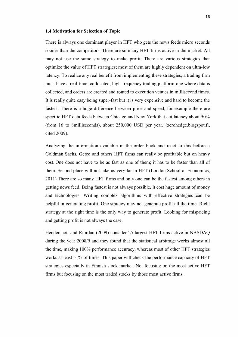
1.4 Motivation for Selection of Topic
There is always one dominant player in HFT who gets the news feeds micro seconds
sooner than the competitors. There are so many HFT firms active in the market. All
may not use the same strategy to make profit. There are various strategies that
optimize the value of HFT strategies; most of them are highly dependent on ultra-low
latency. To realize any real benefit from implementing these strategies; a trading firm
must have a real-time, collocated, high-frequency trading platform-one where data is
collected, and orders are created and routed to execution venues in millisecond times.
It is really quite easy being super-fast but it is very expensive and hard to become the
fastest. There is a huge difference between price and speed, for example there are
specific HFT data feeds between Chicago and New York that cut latency about 50%
(from 16 to 8milliseconds), about 250,000 USD per year. (zerohedge.blogspot.fi,
cited 2009).
Analyzing the information available in the order book and react to this before a
Goldman Sachs, Getco and others HFT firms can really be profitable but on heavy
cost. One does not have to be as fast as one of them; it has to be faster than all of
them. Second place will not take us very far in HFT (London School of Economics,
2011).There are so many HFT firms and only one can be the fastest among others in
getting news feed. Being fastest is not always possible. It cost huge amount of money
and technologies. Writing complex algorithms with effective strategies can be
helpful in generating profit. One strategy may not generate profit all the time. Right
strategy at the right time is the only way to generate profit. Looking for mispricing
and getting profit is not always the case.
Hendershott and Riordan (2009) consider 25 largest HFT firms active in NASDAQ
during the year 2008/9 and they found that the statistical arbitrage works almost all
the time, making 100% performance accuracy, whereas most of other HFT strategies
works at least 51% of times. This paper will check the performance capacity of HFT
strategies especially in Finnish stock market. Not focusing on the most active HFT
firms but focusing on the most traded stocks by those most active firms.
Page 17
17
Although there are so many researches done in HFT strategies, there is still a gap in
the performance capacity evaluation of those strategies. This paper will try to fill that
gap. Strategies are the technical way to get profit from the investment. They differ as
per time and other characteristics of the assets and the firms. Profit from the strategy
is time dependent and same strategy does not work every time.
This paper will try to find the time dependency of different HFT strategies in Finnish
Stock Market. The capacity of the trading strategies will be evaluated based on the
comparative ratios and again cross checked with the market inefficiency. Sometimes
strategies seems to be working even if they are not so effective, which can be due to
market inefficiency.
Most of the active members in Nordic and Finnish stock market for HFT are the
firms that are based on the outside of the Finland. Finland is one of the best
technologically advanced nation but still there are not sufficient HFT firms. Most of
the HFT activities are done by the firms those are based outside of Finland. This
thesis will be helpful to those who are willing to involve in HFT activities in the
Finnish stock market and unaware of what strategy is best for Finnish stock market.
Cartea et al (2011) have distinguished two types of market orders as influential and
non-influential. This thesis will look for the influence of HFT activities in LOB after
excluding non-HFT activities in selected Finnish stocks. Pragma (2012) and Kearns
et al (2010) empirically show that profit generated by most of the HFT firms is
centered to few highly liquid stocks. We will check either similar situation exists
with Finnish stocks or not.
This thesis will be the first paper to analyze the performance capacity of HFT trading
strategies in Finnish stock market using comparative ratios and market inefficiency,
empirically.
Page 18
18
1.5 Research Questions
Since the motive of this thesis is to study the performance capacity of HFT strategies
in Finnish Stock market based on comparative ratios, we will find the ratios of
different HFT strategies. Strategies are differentiated based on their holding period as
suggested by Aldridge (2009). To make sure either they are HFT strategies whose
capacity generates alpha or it is because the market is inefficient, this paper will
cross check the inefficiency of the Finnish stock market. The main research questions
of this thesis are;
Main Research Question
What is the performance capacity of HFT strategies in Finnish Stock
market?
Sub Research Questions
Is the Finnish stock market inefficient?
Strategies are efficient or the market is inefficient?
Does same strategy be profitable for all the stocks?
Are HFT strategies, time dependent?
Which HFT strategy works better in Finnish Stock Market?
Hypothesis to be tested
HFT strategies are dependent on time and stock selection as profit (α)
generated using same strategy for all the stocks for all the time is not
statistically significant.
Null Hypothesis (H0) α=0
Alternative Hypothesis (H1) α ≠0
The first goal of this study is to explore the hypothesis thorough manner, both
through statistical analysis and through proving it using empirical data. Though,
Aldridge (2009) has given the basis for measurement of performance capacity of
HFT strategies, but no research is found to apply her suggestions empirically. This
paper will try to give some empirical evidence to those strategies.
As the argument by Skouras & Farmer (2013), the only thing that is the most
effective in HFT to generate profit is the speed advantages through the co-location of
server near the exchange not the strategies. This paper will try to find out whether the
different strategies used in different times among different stocks are enough to get
alpha from the trading or not.
Page 19
19
2. THEORITICAL FRAMEWORK
This section, first deals with the definition of key concepts such as HFT, and AT and
further explains other related terms of HFT, chosen for this thesis. What are different
HFT strategies and how those strategies are evaluated is the main concern of this
section. It provides a review to previous empirical studies done by the scholars in
HFT and HFT strategies, evaluating HFT strategies, where the most important
findings, opinions, and the research gap is discussed as a literature review.
2.1 Definition of HFT
One must be familiar with Algorithmic Trading to understand HFT. AT uses the
computer algorithms to make automated trading decisions, submit orders, and
manage orders after submission (Hendershott & Riordan, 2009).
Aldridge (2009) characterizes HFT as;
Short position-holdings (seconds, minutes or hours but less than a day)
No or small overnight positions
A large number of trades with a small profit per trade
Analysis of tick market data
These days the latency of HFT is calculated in microseconds. Seconds is way too
long period for high frequency traders. Generally the position which stays overnight
is not considered as high frequency activity. HFT is all about the combination of
mathematics and technology. Many financial professionals say that there is nothing
to do with finance guys in HFT. Since it is all about speed and the complex
algorithms to capture market inefficiencies, the built in algorithms can do such
analysis which is bringing controversies in HFT.
U.S. Securities and Exchanges Commission attribute certain specific characteristics
of HFT and they are;
Use of highly sophisticated computer programs for placing and executing the
orders.
Use of co-located servers to get individual data feeds from the exchange with
very low latency.
The holding period of the position is less than a second.
High orders submission but low executions.
Page 20
20
The description of HFT in case of Aldridge and U.S Securities Exchange
Commission is little bit different in terms of holding period of the securities. U.S
Commission takes into account the less than one second holding period as high
frequency where Aldridge says high frequency trading holding period can be less
than a day as well.
Gomber et al. (2011) states seven common characteristics of AT and HFT, such as;
pre-defined trading decisions, use by professional traders, observing market data in
real time, automated order submission, automated order management, no human
intervention, and use of direct market access.
2.2 Difference between HFT and Algorithm Trading
The best way to differentiate HFT from AT is to understand that, “All HFTs are ATs
but ALL ATs are not HFTs”. There are many similarities between HFT and AT.
Sim
ila
riti
es
Characteristics HFT AT
Automated order
submission and
execution
Real-time data
Direct/sponsored
market access
Dif
feren
ces
Order frequency Very high Varies
Holding period Typically less than a
minute but depends upon
the strategy.
It can be days, weeks or
months depending upon the
trade size.
Latency
sensitivity
Extremely high Varies
Instruments Focuses on highly liquid
securities.
Varies
Table 2: Similarities and differences between HFT and AT (Source: Aldridge 2009)
Page 21
21
It is sometimes difficult to distinguish HFT from AT. To have better concept on HFT
it is first necessary to have knowledge on AT. HFT and AT differs to each other in
terms of holding period. AT might have holding period more than a trading day
where as HFT has no overnight position.
Figure 5: Real time trading model with data flow of prices and deal recommendations (Source: Gençay et al.2001: pg. 298)
Market - Time
Current Return Calculator
Current Return
Gearing Calculator Stop-loss Detector
Gearing Gearing
Recommendation Maker
(Deal Filter)
Recommendation
Simulated Trader
Position Maker
(Opportunity Catcher)
Position
Book- keeper
(Cost Calculator)
Position + Cost
Simulated Trader Statistics Performance
Calculator
Historical Statistics
Model Statistics
Simulated Position
Display Users
Trading Model
Warning signal
To users
TM
Portfolio
Filtered Quotes
Page 22
22
The trading model of any securities largely depends upon the quality of data feed
receiving from the exchange. Any applications either it is forecasting or other trading
application models can perform better with the qualitative data. Bad or incomplete
data can be very harmful to the traders. Real time trading models used the high
frequency data feed and reacts to it instantly. Real time trading model is usually high
risk and high return model. HTFs are the subset of Real Time Trading (RTT). We
can say, “All the HFTs are RTTs but all the RTTs are not HFTs.” High frequency
traders use the real time tick by tick frequency level data. HFT firms use real time
trading models to capture the spread and the arbitrage from the pricing error. The real
time trading strategy model must have the following characteristics; prior warning
mechanism,
Consistency in recommendations,
Recommendations within business hours,
No recommendations in holidays, and
Real time, stop loss support mechanism.
Based on the pre-determined model, the real time trading model must give
recommendations consistently to the portfolio manager. Recommendations have to
be within the business hours when there is possibility of trading the securities. The
trading model must be pre-programmed about the business hours and the holidays so
that it can give recommendations when needed. All the HFT strategies have the
capacity of performing real time trading. All the strategies should be able to have real
time stop loss mechanism. Profit generating capacity of the strategies can be helpful
in generating money but sometimes if the strategies are not built with stop loss
mechanism than it might be dangerous to the trading firm. The incident like Flash
Crash9 of 2010 can make the trading firm insolvent if they do not have the stop loss
mechanism in their trading strategies. One should be aware of possible loss while
thinking about the possible gains. Target limit or stop loss are the tools that always
help in retaining profit and saving the traders from big hazards of loss. All the HFT
strategies also follow these real time trading principles. HFT strategies are more
complicated than the normal real time trading strategies so that they can capture
profit in complex and high speed environment.
_____________________________ 9Flash Crash is the quick drop and recovery in the price of securities that occurred on May 6, 2010
shortly after 14.30 Eastern Standard Time. Although the security exchange commission report gives
several reasons but the real reason is still unidentified.
Page 23
23
2.3 HFT Strategies
Market must be highly liquid to apply the HFT strategies. Similar HFT strategies can
be applied to different markets like, equities, foreign exchange, futures, options and
other derivatives. HFT strategies benefit society in so many ways, such as;
Increased market efficiency
Added liquidity
Innovation in computer technology
Stabilization of market systems
Since HFT strategies require shorter evaluation period because of their statistical
properties, they may not be suitable for long term portfolios. Many HFT strategies
provide liquidity to the markets making markets smoother with less frictional costs in
the heterogeneous market there may not be one best strategy that is fruitful all the
time. It depends upon the stock selection, time and situation as well as the trading
and risk profile of the investors.
Strategy Description Typical Holding
Period
Automated Liquidity
Provision
Quantitative algorithms for optimal
pricing and execution of market
making positions
< 1 minute
Market Microstructure
Trading
Identifying trading party order flow
through reverse engineering of
observed quotes
< 10 minutes
Event Trading Short-term trading on macro events < 1 hour
Deviations arbitrage Statistical arbitrage of deviations
from equilibrium: triangle trades,
basis trades, etc
< 1 day
Table 3: HFT Strategies (Source: Aldridge, 2009)
Basically HFT strategies differ as per the holding period they use as well as the
trading mechanism they use while trading the securities. Aldridge suggests these four
different HFT strategies for high frequency traders. Aldridge (2009) includes three
different HFT strategies as; Electronic market making, Statistical Arbitrage and
Liquidity detection.
Page 24
24
2.3.1 Liquidity provision or Market making strategy
Market making strategy is a mechanism of generating profit from bid and asks spread
of the securities. This is also known as passive market making strategy. This strategy
mimics the traditional role of market makers. After the immergence of HFT firms the
liquidity of the market has increased along with decrease in bid-ask spread. To make
money from the spread market makers quote offer price above the market price and
bid price below the market price. In HFT the bid and ask quotes are generated
automatically by using limit order via complex algorithms. Some HFT firms use
pinging10
to place limit orders so that they can quickly withdraw their orders before
execution. Market makers are not obligatory to quote the market, so the lack of this
formal obligation may reduce the liquidity when it is needed the most.
Figure 6: Basic sequential trade model (Source: Joel Hasbrouck, 2007, pg. 44-47)
Bid-Ask spread is
In a symmetric case of = ½, A-B=
__________________________
10 pinging is a technique to enter into market through small marketable orders in order to learn about
the large hidden orders hidden in exchanges.
Buy
Sell
Sell
Sell
Sell
Buy
Buy
Buy
0
1
1/2
1/2
1
0
1/2
1/2
I
U
U
I
V’
V
V
μ
1 - μ
1 - μ
μ
δ
1 - δ
Page 25
25
The tightness of bid and ask spread can be measured continuously over the trading
day using a simple method;
Tightness of Trading Spread= (Ask Price - Bid Price) / Bid Price
In this method an average time weighted spread is used to see the tightness of the
spread. This technique would not be able to define the tightness of the spread if the
two way quotes is missing. In tangible assets, market becomes tight when there is
more demand than the supplies or the imbalance in-between demand and supply.
Similarly, in intangible assets market, there are plenty of buyers and sellers in all the
time which leads in the decrease in bid-ask spread. Market makers place limit orders
on the buy side as well as sell side of the order book. They are responsible for
providing liquidity for market orders. Market makers earn the spread between bid
and ask by providing liquidity to the market. Market makers are also taking risk and
there is the possibility that they will lose money with better informed counterparties.
Market makers update their bid and ask price frequently based on the new market
information, new order submissions and the cancellations.
HFT market makers are one of the counterparties of the normal market makers or the
clearing members. They act little differently than the normal clearing members. They
tend to place large numbers of add order to the limit order book and immediately
cancel the same orders before executions of those orders. HFT market makers have
replaced traditional market makers in recent dates. Traditionally market makers were
used to be a human now market makers are more technologically advanced
computers than humans. It is beyond the capability of humans to provide liquidity to
high frequency traders manually. In most equity markets, liquidity providers also get
liquidity rebates. Liquidity rebates is also known as market makers’ fees.
There is another mechanism of providing liquidity which is also known as ‘Make or
Take’ pricing. Where, this clearing member provides liquidity to outstanding limit
orders placed by the customer, which is very lower or higher than the current market
price. In return exchange rebates some portion of that access fee to the market
makers as liquidity rebates. Market making strategy in HFT is challenging to get
spread out of bid and ask as the spread might be lower than the transaction fees.
Hagströmer and Norden (2012) show that NASDAQ OMX Sweden accounts around
72% of marketing making strategy among 86% of HFT Limit order data.
Page 26
26
2.3.2 Market Microstructure trading
Market microstructure is the study of the process of exchanging assets under explicit
trading rules. Market microstructure analyses about how some specific trading
mechanisms affect the price formation process of a security. This price formation
mechanism may include some intermediaries such as finance specialist, or exchange
or some electronic interface. Market microstructure enhances the ability to show
how different trading mechanism affects the trading protocol and price formation.
How price exhibits certain time series properties. This helps in understanding the
return generated by the financial assets as well as the efficiency of the market
(Maureen O’Hara, 1995).
Joel Hasbrouck (Empirical market microstructure: 2007, pg. 7) provides the list of
significant outstanding questions in market microstructure:
What are the optimal trading strategies for typical trading problems?
Exactly how is information impounded in prices?
How do we enhance the information aggregation process?
How do we avoid market failures?
What sort of trading arrangements maximize efficiency?
What is the trade-off between “fairness” and efficiency?
How is the market structure related to the valuation of securities?
What can market/trading data tell us about the informational environment of
the firm?
What can market/trading data tell us about long-term risk?
In this thesis we will answer some of the above questions. Market microstructure
data are distinctive time series. In high frequency tick data generation, the
millisecond time interval is not homogeneous. Tick price generation time interval
from previous to the current and upcoming from current tick price is different.
Highly liquid securities have less time interval in-between two tick price. Market
microstructure shows the behavior of price and the market. Over the last decades,
sophisticated automated technologies has created a new era in the world of electronic
trading making micro-structure a very important tools to be understood in order to
formulate HFT strategies. Price reversal strategy is one of the market micro structure
strategies where the traders will try to reverse the price of the security by cancelling
the large portion of his orders and by creating order imbalance.
Page 27
27
Market structure has been changed in recent years creating more opportunities for
AT and HFT. Traders can make profit from large buy and sell side orders. HFT can
detect large pool of orders and they can anticipate the change and make profit
accordingly. Sometimes large order detection is difficult if the trader is using some
random strategies but for many HFT it is easier to achieve.
Lillo and Farmer (2004) show that when a trading firm is continuously placing large
amount of orders that can create the imbalances that can be seen clearly as it tends to
decrease the autocorrelations between the trade imbalances. Theoretically one can
find the probability of imbalance direction using some forecasting tools, but in
practical it is too complex. When there is diverse effect on the stock and its sector
wise index that can be the indication of large orders by the HFT firms. This
mispricing between the sector wise index and the particular stock of that sector can
be the lead to the HFT and can get huge amount of profit. Some aggressive traders
can easily anticipate the flow of large orders whereas passive investors can play the
role of liquidity provider only. There is still some research gap to show that either
HFT are engaged in order anticipation or not.
Baron et al (2012) empirically show that the profitability of aggressive HFT are
usually higher than the inactive or passive HFT firms. Order anticipation can be done
by the most active HFT firm who is getting news feeds microsecond sooner than
other competing HFT firms, but it comes in a huge cost which is beyond imagination
for normal HFT firms. To avoid the situation of easy anticipation HFT firms usually
place their orders in small order sizes so that it will be difficult for other investor to
anticipate the possible price change from the large order imbalances. It is even more
difficult for market makers to minimize the impact created by the large flow of
orders. When there is normal amount of trades flow with small trade volumes, it will
be even more difficult for passive investors to anticipate the price change. Many
HFT firms cancel their order before execution which makes market maker even more
challenging but these days market making is also automated and it uses its own
strategy for order detection. Since HFT firms are also acting as market makers it is
rare to have order imbalance in the trading day. We can see some order imbalance in
the opening and closing hours of the trading day but they are also there temporarily.
Page 28
28
2.3.3 Event Trading
Sometimes market may take longer time to convey new information. There might be
extremely active trading before and after the major announcement by the particular
firm. The variation in the trading uncertainty is managed by the basic trading model
at the starting of each business day and a random step can be added to capture the
major event information (Easly and O’Hara, 1992).
Figure 7: Event tree at the start of the trading day (Source: Easly & O’ Hara, 1992, pg. 51)
With fast and real time news reporting system, traders now can take the advantage in
real time. Algorithms are written in such a way that it can differentiate the bad news
from the good news. If the event is good (bad) for the stock, then the stock price of
that particular firm will increase (decrease) so the algorithm trades accordingly.
Easley et.al (1996) suggested a model to determine the probability of an informed
trading of the particular asset. Where
α= information event that is observable to some of the traders
1-α= probability of not having any information events
δ= probability of that information event which affects the value of the asset
negatively
1-δ= probability of that information event which affects the value of the asset
positively
V
V’
Information event
No inf. event
Start
I
U
I
U
Buy
Sell
0
1 No trade
Buy
Sell
0
1 No trade
U
Buy
Sell
0
1 No trade
Prior to trading During the trading day
Sell
Buy
Page 29
29
Both the informed and uninformed investors make trades and the arrival rate of the
order is ε. The arrival rate also follows a process, μ. Uninformed traders makes
random decision on trades on their own psychological and analytical basis whereas
informed trades will place the orders according to the nature of the information. If
they have positive information they will buy and, sell if they have negative
information.
Easley et. al (1996) show that the probability that a trade that occurs at time t is
informed is given by;
Where Pn (t) is the probability of a “no event day” at time t.
Event trading is also known as directional trading or news based trading. Machines
these days are programmed to read news. It analyses that good words and the bad
words in the news and does the trading accordingly. Positive news with positive
words like, increase, raise, promoted, higher can suggest the computer to buy the
security for possible increment in the price of the security.
Many news agencies nowadays sell news to the HFT firms for sending them news
prior to the release. This makes HFT firms aware of the possible event in advance
which can be profitable, but relying too much on news agency might be harmful.
Sometimes news is created by the news agencies it selves.
Hendershott and Riordan (2009) consider 25 largest HFT firms active in NASDAQ
during the year 2008/9 and they found out that, each HFT firm earns average $2,351
per stock per day. They found that the statistical arbitrage works almost all the time,
making 100% performance accuracy, whereas most of other HFT strategies works at
least 51% of times.
News based trading uses textual information, its degree of importance, direction of
the effect and potential outcome to do the trading. Information leakages from the
employee to the HFT firms are threads to the exchange as they already know the and
anticipate the effect of the news before it releases and they wait the right time of
news flash and they initiate the trading capturing lots of profit.
Page 30
30
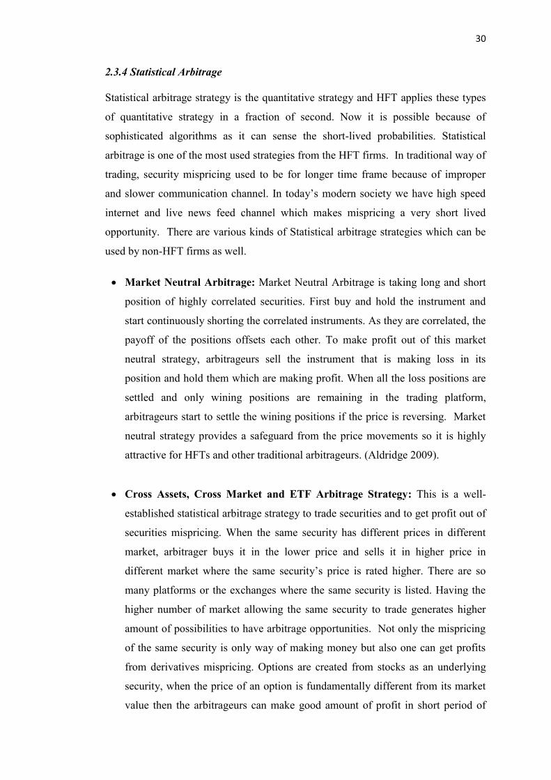
2.3.4 Statistical Arbitrage
Statistical arbitrage strategy is the quantitative strategy and HFT applies these types
of quantitative strategy in a fraction of second. Now it is possible because of
sophisticated algorithms as it can sense the short-lived probabilities. Statistical
arbitrage is one of the most used strategies from the HFT firms. In traditional way of
trading, security mispricing used to be for longer time frame because of improper
and slower communication channel. In today’s modern society we have high speed
internet and live news feed channel which makes mispricing a very short lived
opportunity. There are various kinds of Statistical arbitrage strategies which can be
used by non-HFT firms as well.
Market Neutral Arbitrage: Market Neutral Arbitrage is taking long and short
position of highly correlated securities. First buy and hold the instrument and
start continuously shorting the correlated instruments. As they are correlated, the
payoff of the positions offsets each other. To make profit out of this market
neutral strategy, arbitrageurs sell the instrument that is making loss in its
position and hold them which are making profit. When all the loss positions are
settled and only wining positions are remaining in the trading platform,
arbitrageurs start to settle the wining positions if the price is reversing. Market
neutral strategy provides a safeguard from the price movements so it is highly
attractive for HFTs and other traditional arbitrageurs. (Aldridge 2009).
Cross Assets, Cross Market and ETF Arbitrage Strategy: This is a well-
established statistical arbitrage strategy to trade securities and to get profit out of
securities mispricing. When the same security has different prices in different
market, arbitrager buys it in the lower price and sells it in higher price in
different market where the same security’s price is rated higher. There are so
many platforms or the exchanges where the same security is listed. Having the
higher number of market allowing the same security to trade generates higher
amount of possibilities to have arbitrage opportunities. Not only the mispricing
of the same security is only way of making money but also one can get profits
from derivatives mispricing. Options are created from stocks as an underlying
security, when the price of an option is fundamentally different from its market
value then the arbitrageurs can make good amount of profit in short period of
Page 31
31
time. Similarly exchange traded fund can be mispriced sometimes, as this kind
of pricing inefficiencies last for short period of time, HFT firms use their speed
to capture these kinds of opportunities. (Aldridge 2009). Essential factors in
constructing Statistical Arbitrage strategy are (Quant Congress USA, 2011);
Proper and diversified selection of stocks/options/ETFs
Captures the bid and ask spread
Apply pairs trading according to the model
Manage risk using real-time Value at Risk
Execution using value weighted average price
Avoid taking trading volume into consideration
Statistical arbitrage attempts to bet on the convergence and the divergence of price
movements of pairs and baskets of assets, using statistical methods. The modern
definition of statistical arbitrage is to spread the risk of a single trading among
millions of other trading in a very short holding period, aiming for profit using the
law of one price fundamentals.
A pair trading is one kind of market neutral statistical arbitrage strategy in HFT.
Pairs trading can be based on two-stage approach, one is called correlation approach
and the other is called co-integration approach. This type of statistical strategy is
used to capture the statistical mispricing between pair based stocks.
These days, programmers, engineers and statisticians and many other interested are
making complex algorithms for HFT to squeeze out every penny of returns possible.
Many of the trading strategies are based on the intuition and the psychological state
of mind of the trader rather than based on empirical analysis.
In statistical arbitrage using correlation for pairs trading is one of the tools. Price of
the securities is correlated if they share same news.
Positively Correlated: If same news is good for both and has positive
price movements.
Negatively Correlated: If same news is good for one and bad for
another.
Not Correlated: If one news is good or bad for one and neutral for
another
Page 32
32
Statistical arbitrage is a popular HFT strategies used by hedge funds and other
trading houses. Statistical arbitrage uses cointigration to identify profitable trading
opportunities. It attempts to get profit from the relative mispricing based on the
historical price patterns. Arbitrage usually is riskless but statistical arbitrage is not
riskless.
Ross (1976) Arbitrage Pricing Theory and the cointigration approach are related to
each other. This strategy is also related to Law of one Price. If the two securities
have similar cash flow trends then the price formation of those two stocks are
expected to be similar.
Page 33
33
2.4 Evaluating performance capacity of HFT strategies
2.4.1. Basic return characteristics
There are various kinds of trading strategies in high frequency finance and the most
common motive of using these strategies is to generate profit applying them. Return
can be measured in different time frequency like seconds, minutes, hours, days, years
and longer. There are various performance measurement techniques to evaluate the
basic return characteristics of these strategies. Most of the firm uses annual average
return as a performance measure. All the trading firms prefer higher return. Average
annual return, standard deviation, volatility and maximum drawdown, skewness,
kurtosis are some characteristics for comparison between different strategies
(Aldridge, 2009).
2.4.2. Comparative Ratios
Average return, standard deviation, skewness, kurtosis and other measure the basic
return characteristics of the particular strategy. There are various comparative ratios
which summarize the basic return characteristics. One of the most used ratios is
Sharpe Ratio.
The comparative ratios used in this thesis are Sharpe, Omega, Sortino, Kappa, VAR
and CVAR. Following are the comparative ratios suggested by Aldridge (2009)
Sharpe Ratio: The Sharpe ratio is also known as return, per unit of risk often
represented by variability, sometimes the unit of risk might be the standard
deviation of the returns. Risk and return can be represented graphically. Generally
return is dependent upon the level of risk taken, so return is shown in y-axis and
risk is shown in x-axis.
Risk averse investors always look for high return in low risk. Sharpe ratio
measures the risk and return performance. Higher Sharpe ratio shows the better
performance of the portfolio. Sharpe ratio measures the gradient of security
market line from the risk free rate.
Modigliani (1997) proposes an alternative risk adjusted return using Sharpe ratio,
where the risk factor is the benchmark portfolio and allow direct comparison.
Sharpe ratio helps in ranking the fund based on the order of preference. Ratios of
the investment strategies can be grouped in two different categories such as;
Sharpe type ratios where risk and return, risk adjusted return suggested by
Page 34
34
Modigliani (1997) and the next category is descriptive statistics, where the ratio
only can provide the pattern of the return but cannot suggest either the return is
good or bad. The only thing is, investor prefers lower volatility, lower variance
but the higher average return. Many investors also look at the tail of the return
distribution. They prefer positive skewness along with lower kurtosis. Pezier
(2006), suggest an adjusted Sharpe ratio which rewards positively skewed and
lower kurtosis and thus able to satisfy the criticism of Sharpe ratio.
Treynor Ratio: Treynor ratio is similar to Sharpe ratio but the measure of risk in
Treynor is the systematic risk only. In Sharpe ratio, total risk is used as a risk
measure to calculate the reward to risk ratio. Many portfolio managers avoid
using Treynor ratio because it ignores the specific risk factors. Treynor Ratio is
developed by Jack Treynor. It measures the excess return over market return
which could have been earned on a riskless investment per each unit of market
risk.
Jensen’s Alpha: Jensen’s alpha is another useful performance analytics; it shows
the excess return adjusted for systematic risk. Many times Jensen’s alpha is used
wrongly as the investment manager’s performance over benchmark portfolio. It is
a risk-adjusted performance measure that calculated the average return on a
portfolio over the predicted return by the Capital Assets Pricing Model.
Omega: Shadwick and Keating (2002), suggest a ratio called Omega that gives
the information in the higher moments of a return distribution. Omega is also
known as gain-loss ratio which implicitly adjusts both skewness and kurtosis,
considering upside and downside potential.
Sortino Ratio: Sortino (1991) suggests an extension of Sharpe and Omega called
Sortino ratio which uses downside risk as the risk factor in the denominator. Since
upside return movement is good for the investors, it only takes downside return
movement as risk factors. So, in Sortino ratio, the total risk is simply replaced by
the downside risk.
Calmar Ratio: The Calmar ratio is a Sharpe type measure, which uses the
maximum drawdown rather than total risk. If lower the Calmar Ratio, the worse
Page 35
35
the strategy performance on a risk adjusted basis, similarly higher Calmar ratio
suggests better strategy performance. It is developed by Terry W. Young (1991).
Calmar ratio is typically based on recent and short-term data.
Appraisal ratio: Treynor and Black (1973) suggest appraisal ratio which uses
Jensen’s alpha. They use systematic risk adjusted excess return divided by the
specific risk factors which measures the systematic risk adjusted return for each
unit of specific risk taken.
Sterling Ratio: The Sterling ratio replaces the maximum drawdown in the
Calmar ratio with average of largest drawdowns. This ratio is mainly used by the
hedge fund managers. It determines which hedge funds have the highest returns
with less volatility. Similar to Calmar ratio, higher sterling ratio is better which
means that investment strategies are making higher return relative to risk.
VaR (Value at Risk): VAR is a statistical technique which measures and
quantifies the level of financial risk. Many investment managers use VAR to
measure and control the level of risk that firms undertake. The job of the
investment manager is to ensure that risk taken by his firm is not beyond the level
which firm cannot absorb the losses of a probable worst case scenario. Value at
Risk measures three things, the potential loss amount, probability of that loss to be
occurred, and the investment time frame. All these ratios are very familiar for
portfolio managers. Recently hedge funds are using more risk associated with
different types of investors. Value at Risk (VaR), is also a Sharpe type measure
where total risk is replaced by the VaR.
CVaR (Conditional Value at Risk): Conditional value at risk is also called
expected shortfall. As similar to Conditional Sharpe, in Conditional VaR,
conditional variance is replaced by conditional value at risk. VaR is unable to
provide the information about the size and shape of the tail, thus it is not so good
measure of risk for many investors. Conditional VAR overcomes this drawbacks
and it can give the expected shortfall, expected mean loss and the shape of the tail.
Page 36
36
2.4.3. Performance Attribution
Attribution analysis aims to differentiate between selection strategy and market
timing strategy on the superior performance of the portfolio. This analysis compares
the actual return of the investment manager with the predefined benchmark.
Attribution analysis subdivides the actual return into selection effect and allocation
effect. Performance attribution is also known as investment performance attribution.
It is used to describe why some portfolios outperform the benchmark. Investor with
active trading strategies can outperform the benchmark where as for the passive
investor it is hard to outperform the benchmark. There are various kinds of
attribution analysis for various kinds of portfolios. Active portfolios and passive
portfolios use different methods in explaining the performance attribution.
Attribution is also known as benchmarking. Various scholars like, Ross (1977),
Sharpe (1992), Fung and Hsieh (1997) applied performance attribution analysis to
trading strategy. Doing regression of various factors into one basket of the factors
with strategy’s return is a way to get performance attribution of that particular
portfolio, Aldridge (2009).
Where,
bk measures the performance of factor k.
αi measures the persistent ability generating abnormal returns, and
μit measures the idiosyncratic return of the strategy in time period t.
Fung and Hsieh (1997) use eight global groups of asset classes to set as a
performance attribution benchmark. Performance attribution is a good measure of
return generated by applying the strategy. It shows the investment styles and the
design of the investment strategy. It gives grounds for comparison between different
other strategies. Performance attribution helps in forecasting strategy performance
(Jagadeesh and Titman, 1993).
2.4.4. Other Forms of Strategy Evaluation
Strategies are time dependent. Same strategy may not be profitable in all kind of
situations. Though there are so many other strategies with different names, the main
goal of them is to make profit. Some makes profit from the bid ask spread using
Page 37
37
market making strategy, some uses quantitative strategies like statistical arbitrage to
make profit. Buying in lower price and selling in higher price is not the only way to
make profit these days. Capacity of each strategy is measured based on their
performance over benchmarking. Other form of strategy evaluation includes;
Strategy Capacity: Strategy selection can be based on the amount of investment
and the liquidity of that instrument. Placing large amount of orders is also not
considered good if there is liquidity problem. In HFT strategies are used to
capture the ounce from every trade which is not seen significant if treated as a
single trade but when multiply it with the huge amount of trade volumes then
every second there is high amount of profit generation.
Length of the Evaluation Period: There is always a question about selecting
the best evaluation period. Long term investors basically like to consider longer
time period into consideration while short term investors see the price
movements in the short period of time. Long evaluation periods generally means
the period between six months to two years where short period is considered to
be an intraday period up to one month. The higher the value of Sharpe ratio, the
shorter must be the evaluation period to assure the validity of Sharpe ratio
(Aldridge, 2009).
Autoregression-Based Test: If the market is efficient it is harder for the
investment managers to make strategies which lead them to huge amount of
profits. Trading strategies work better in the least efficient market. In perfect
efficient market, prices reflect all the current available information, thus
suggesting no dependencies from past price movements. Explanatory power of
past price is one way to measure market efficiency. Mech (1993) and Hou &
Maskowitz (2005) give one effective measure to find the market efficiency by
finding the difference between Adjusted R-Squared coefficients of restricted and
unrestricted model. The main difference between restricted and unrestricted
model is that, restricted model restricts all coefficients of beta to be zero.
Inefficiency close to zero shows market is efficient and close to one shows
market is inefficient.
Market Inefficiency= 1- [R2
(Restricted) / R2 (Unrestricted)]
Page 38
38
2.5 Literature Review
Many HFT strategies use the speed advantage as they can process information, make
orders in a very short period of time in very large scale. Cartea et al (2011) have
distinguished two types of market orders as influential and non-influential. If any
orders affect the shape and dynamics of LOB then the orders are influential where as
if the orders have no any effect in LOB then they are non-influential. This thesis will
look for the influence of HFT activities in LOB after excluding non-HFT activities.
Kumar et al (2011) show that, US has over 70% HFT activities in equity market and
European equity market has around 40% HFT activities. Asia is also in increasing
phase and it has around 10% of HFT activities. The increasing popularity of HFT in
Asia in recent days can make the Asian stock market more active and volatile. In this
thesis, the influence of HFT in Finnish stock market will be studied. Cartea et al
(2011) have another contribution in optimal high frequency trading strategy. They
model short-term alpha in the drift of the mid-price as a zero-mean reverting process.
The drift fluctuates randomly when there are influential orders in the order book or
some event driven trading. Since the same stock can be traded globally, any incident
in one part of the globe can create chaos in another part of the world. Event is an
important hint for HFT traders. They always seek for some major events which are
not yet confronted towards the public by any public channels or media. Market event
has an important impact in the arrival of influential orders. Market news can be good,
bad or ambiguous. As per the nature of the news order submission on buy or sell side
is determined by the traders. Good news generally increases the value of the firm so
traders prefer to buy and sell if the news is bad. If the event is ambiguous then
traders can apply market neutral strategy.
(Almgren and Chriss, 2000) is one of the most widely used models for execution
strategy. A key input for execution strategy is the length of execution horizon. This is
typically set as exogenous, with an estimate. The execution horizon may differ as per
the strategy used but sometimes HFT firms uses the same order duration and holding
period horizon. Using dynamic strategies will differentiate between the gains and
losses and lengthen its horizon to capture the profit. Kearns et al (2010) empirically
show that profit generated by most of the HFT firms is centered to few highly liquid
stocks. Individual investor can wait for their price level but it is difficult to complete
trades in certain price time priority. To overcome this kind of situations HFT firms
Page 39
39
use highly aggressive strategies with some cost. HFT in such securities can be
profitable using aggressive trading styles. There is chances of high bid and ask
spread as well. If there is large amount of market orders in the queue then those
orders can be absorbed in the same price level. Pragma (2012) shows that HFT firms
are concerned in the most liquid stocks only, as they can take the advantage of high
speed price change or the tick price. We will check the concern of HFT firms on
Finnish stock market. Highly liquid stocks sometimes experience crowding from the
market maker and it is difficult to determine the best bid/ask price. Easley et al
(2011) state that speed is not always the advantage for HFT firms, since they use
volume time instead of chronological time. Skouras and Farmer (2013) say that
besides any effective HFT strategies, HFT firms use their speed advantages to be
ahead of the queue among other market participants and manipulate the market.
Leinweber (2009), Technological advancement is not only making it easy for HFT
firms to get profit by employing their strategies and speed but also it is making them
difficult as their counter parties are also using the same level of technology.HFT
firms use the benefit of speed so that they can place and withdraw their position from
the limit order book. If they are not been able to cancel their position in current
market price that will create market liquidity risk. Bervas (2006) states three different
criteria to measure the liquidity and they are;
Tightness of bid-ask spread: Bid-ask spread identifies the cost of
immediate reversal of the position
Market depth: It is the volume of that particular security which can be
bought or sold in the same best selected price without price slippage.
Market resilience: It measures the speed of price reversal to equilibrium
price after a significant increase in order flow.
The optimal HFT strategy shows how to optimally submit orders, optimally
determine the cancellation and execution rate based on the news or the market
events. Optimal HFT strategy helps in identifying HFTs from AT based on the
characteristics of the trades. Cartea et al (2011) test their model using simulations
where they take that information which can be processed and incorporated in sending
optimal trading orders. Many HFT orders are withdrawn from the market as the limit
orders are driven by the better informed traders. They also show that those who are
unable to make profitable strategies can systematically stay in business if they have
enough controls over their inventories. Cartea and Penalva (2010) suggest “spoofing”
Page 40
40
where the traders send a large pool of orders in either side of the limit order book and
after triggering the opposite side of the order book they immediately cancel the
orders and place the orders in other side of the limit order book. Aldridge (2009) says
that, HFTs mostly follow the highly liquid stocks; this is because of tick data
generation time interval. Highly liquid stocks generates tick price regularly in a very
short time interval. This will help high frequency traders to trade in time volume.
Heston et al (2010) show that though different HFT firms use different HFT
strategies but institutional HFT investors leave a noticeable pattern in their trading
activities which makes it easier to copy the HFT strategies. Barber et al (2009) state
that, retail HFT are usually the noise traders and they trades in a very small
fragments and so it is difficult to detect the trading pattern of retail HFT traders. We
will check the higher order fragmentation on all the selected stocks. Hagströmer &
Norden (2013) emphasizes how different HFT strategies influences on market
quality. They focus particularly on market making strategy on NASDAQ OMX
Stockholm market. This thesis will check market marking and other strategies on
NASDAQ OMX Helsinki. Gencay (1998) states that, the ultimate goal of any HFT
strategy is to generate profit. Sandro et al (2008) study the trading imbalances and
the predictable price reversals. They find that imbalances generate predictable
reversal in stock return. Any imbalances in one security affect the trade balance of
another stock as well. The net order imbalance is seen only at the very beginning and
very ending of the trading day. These types of orders imbalance do not necessarily
create price reversal. It might affect the opening price of next day’s. Chordia et al
(2000) find the impact of order imbalance in liquidity and market returns. They
studied with the data from New York Stock Exchange. They show how order
imbalances in any direction either buy or sell reduces the liquidity of the market.
Traders may be able to control the volume and liquidity but market return is always
affected by the net order imbalance, suggesting market micro structure strategy as a
tool to generate profit. Reberto et al (2002) empirically show that, not only price and
return are random but also the waiting time between the two transactions also varies
using high frequency data. Generally the waiting time in HFT is determined by the
possibility of converting the position into profit. Waiting time varies from one
position to another and from one stock to another based on the market movements as
well as the possibility of positive return. We will check the order duration to compare
the average waiting time of all the selected stocks.
Page 41
41
3. DATA AND RESEARCH METHODS
This section includes the availability and description of high frequency limit order
data used in this thesis. It provides a clear picture about the structure of high
frequency data sets in a millisecond time interval. The raw data generated by the file
delivery system of NASDAQ OMX includes all of the trading activities. It is in the
hand of the author to consider the required message feed for the primary data sets for
further empirical analysis. Basic limit order book activities are studied for the
selected stocks which includes add, cancel and execution actions. The order
generating pattern and the order imbalance is also studied for each selected stock.
Empirical research methodology in this thesis follows multiple steps to come into
conclusion. First a return series is generated following the respective strategy with
the respective holding period as suggested by Aldridge (2009). Comparative ratios
are calculated based on the return series. Then, this thesis uses the OLS (Ordinary
Least Square) estimation method by using ARMA (Autoregressive Moving Average)
model for the respective return series. Next, for the autoregressive based test for
market inefficiency we identify the restricted and unrestricted R-squared required to
calculate the market inefficiency. Conclusion is drawn based on the significant
excess return, comparative ratios and inefficiency of the return series for each
respective strategy’s holdings for both long and short positions.
3.1. Data Availability
The data used in this thesis is one month high frequency limit order and tick data
from NASDAQ OMX Nordic. The data is generated by Helsinki Stock Exchange
Automated Trading and Information System for the month of November 2013. By
paying the subscription fee to the exchange, data can be downloaded whenever
needed taking into consideration some limitations. File Delivery System (FDS) of
NASDAQ OMX provides the basic data which includes the limit order data. The
ITCH data includes all the order book activities of stocks listed in NASDAQ OMX
Nordic (Helsinki, Stockholm and Copenhagen) exchanges. Since the motive of this
thesis is to study the performance capacity of HFT strategies in the context of
Finnish stock market, we take into consideration the Helsinki exchange only. There
are more than 136 Finnish stocks listed in NASDAQ OMX Helsinki. For the study of
Page 42
42
performance capacity of high frequency trading strategies applied in trading stocks,
this thesis selects six highly traded stocks based on the activities in the limit order
book for the month of November 2013 and the highly traded stocks are; Nokia, Stora
Enso, Nordea, Metso, Outokumpu and Nokian Renkaat.
3.2 Data Structure
NASDAQ OMX Nordic offers data feed in ITCH protocol. ITCH is direct data-feed
such as TCP (Transmission Control Protocol) or UDP (User Datagram Protocol). In
ITCH traders track the status of each order from order generation to its execution or
cancellation. ITCH is mainly for information exchange only. Each information
message length is based on its type. Subscribers can also get administrative
messages if they have proper subscriptions. Messages send using ITCH, use high
level of protocol so that the message is properly sequenced and guaranteed delivery.
There are three different ITCH protocol options used by NASDAQ OMX Nordic and
they are;
SoupTCP: This protocol uses the single outbound channel for all
securities using transmission control protocol.
Compressed via SoupTCP: This protocol also uses the single outbound
channel for all securities via transmission control protocol, but the
protocol option can be offered to the members of exchange.
MoldUDP: This also uses the single outbound channel for all securities
via user datagram protocol.
ITCH is a direct data feed offered by the NASDAQ OMX Nordic with the following
data structure and elements.
Order Level Message: ITCH uses a series of order messages from the
beginning of order generation to the end till its execution or cancellation.
Exchange will provide its full order description using the standard ITCH
protocol.
Page 43
43
Trade Message: ITCH provides separate message to reflect cross
transactions. ITCH supports message that can reflect non-displayable
order in the system to ensure customers have complete information about
the trade flow.
Net Order Imbalance Message: To calculate the best opening and
closing price of the stock at the very beginning and closing of the trading
day, the system calculates the equilibrium price along with the imbalance
direction and quantity. The equilibrium price calculation includes both the
displayable and non-displayable order types. Net order imbalance is
helpful in predicting the best opening and closing price of the security to
the public.
Administrative message: Administrative message includes the trading
actions and symbol directory message. Trading action message informs
traders either the security is available for trading or not, it also shows if
the security is halted or released for trading. Symbol directory message
includes all the basic information about the security such as financial
status.
Event Control Message: This message type includes the trade events
such as the opening of trading day, end of the trading day as well as the
states of the different market segments.
NASDAQ OMX Nordic use separate time stamp message for efficiency reason to its
ITCH product. ITCH provides sequential data feed so that the subscriber can get the
trade message in proper time stamp. Time stamp in ITCH is separated first as second
message and within each second message millisecond message is generated which
includes all the trading action and order level data. For each second nine hundred
ninety-nine milliseconds are generated, when the millisecond touches one thousand it
jumps to next second and the same process continues.
______________________
For more information on the File Delivery System (FDS) of NASDAQ OMX Nordic, see this link:
http://www.nasdaqomx.com/digitalAssets/89/89849_fds_-guideline_20130117.pdf
Page 44
44
3.3 Data Description
Data received from the NASDAQ OMX Nordic from one month subscription
includes the high frequency order level activities generated in ITCH system. The
ITCH message includes the following information need for this thesis;
ISIN: International Securities Identification Number
OrderRefNo: Order Reference Number to identify each unique order placed
in increasing pattern.
BuySell: Indicates either the investor is long or short by indication “B” for
buy and “S” for sale.
Millis: Millisecond time stamp in increasing number. 1000 Milliseconds = 1
Second.
Action: It indicates the particular action in limit order book by the investor. It
includes four different actions and they are;
“A” = Order is added in limit order book
“X”= Order is cancelled from the limit order book
“D”= Order is deleted from the limit order book
“E”= Order is executed
Quantity: It shows the number of buy or sells order added / cancelled /
deleted / executed from the limit order book.
Date: It shows the particular day of limit order book activities in yyyymmdd
format.
ISIN OrderRefNo Buy/Sell L.Price Millis Action Qnty Date
FI0009000681 5242079 S 5.63 45138586 A 4557 20131101
FI0009000681 5242079 S 5.63 45138819 X 957 20131101
FI0009000681 5242079 S 5.63 45138819 X 3000 20131101
FI0009000681 5242079 S 5.63 45144398 D
20131101
FI0009000681 5242080 B 5.615 45138586 A 4000 20131101
FI0009000681 5242080 B 5.615 45138602 X 3000 20131101
FI0009000681 5242080 B 5.615 45138602 E 1000 20131101
Table 4: Nokia LOB sample
Note: Data presentation format is solely in the hand of the author of this thesis. The data feed generated from
ITCH protocol can be read using some programming languages and statistical software.
Page 45
45
4. EMPIRICAL ANALYSIS
In this section we do the statistical analysis of the available data with the pre-
specified methodologies. The empirical analysis part of the thesis mainly focuses on
the three empirical activities of the top six mostly traded Finnish equities listed in
NASDAQ OMX Nordic. At first, the basic limit order book activities of all the
selected stocks including and excluding non-HFT activities will be analyzed. It is to
make sure that all the selected stocks have the influence of HFT traders, so that the
obtained result will be more accurate. The next step in the analysis is to apply the
HFT strategies and the respective holding periods of the strategies to generate the
return series. The return series then follow the ordinary least square method of
estimation using the ARMA model to find out the intercept. The significance of the
strategy is measured from the statistically significant intercept. Different comparative
ratios are calculated for the comparison between the strategies of HFT and non-HFT
traders holding long and short positions. The final step in the analysis cross checks
the inefficiency in the market via autoregressive test.
4.1. Limit Order Book (LOB) Activities
NASDAQ defines Limit Order Book (LOB) as a record of unexecuted limit orders
maintained by the specialist. These orders are treated equally with other orders in
terms of priority of execution (www.nasdaq.com).
Rank ISIN Stock HFT Activities of
that month
HFT Activities 1st
Nov 2013
1 FI0009000681 Nokia 3981326 254130
3 FI0009902530 Nordea Bank 3061289 137108
2 FI0009005961 Stora Enso 2738642 141569
4 FI0009007835 Metso 986465 73641
5 FI0009005318 Nokian 917992 67806
6 FI0009002422 Outokumpu 420762 66452
Table 5: Number of activities in LOB as on November 2013
Note: HFT activities from the limit order book is counted based on the duration of order. If the
particular order is stayed overnight then it is not considered as high frequency order. Order
reference numbers which are not repeated on the same trading days are excluded from the HFT
order book.
Page 46
46
Nokia is the most highly traded Finnish stock listed in NASDAQ OMX Nordic with
highest HFT activities. Nordea share is also traded in the similar manner to Nokia.
The number of high frequency trading activities is decreasing rapidly in each
successive stock. Top three has significant numbers of HFT activities where are other
three has less impact by the HFT traders. But the HFT message generated is clearly
visible in all six stocks.
Stocks Order Duration Max Min
Order Duration Mean Median
Max. Price Min Price Std. Dev
Bid Ask Bid Ask Bid Ask
Nokia 36874.92 0 778.2073 3.368 6.03 6.8 5.11 5.535 0.1161 0.1176
Stora Enso 35524.11 0 552.1229 2.789 7.535 8.02 6.465 6.825 0.1519 0.1493
Nordea 36127.53 0 443.9333 1.969 9.545 10.32 8.235 8.93 0.1616 0.1560
Metso 36890.21 0 696.2625 2.853 30.45 32.14 26.88 28.46 0.3849 0.3862
Nokian 30349.5 0 556.6366 2.086 38.72 41.25 34.31 36.08 0.4797 0.4859
Outokumpu 36892.32 0 868.0858 39.552 4.99 4.5 3.596 3.751 0.0132 0.0123
Table 6: The most traded Finnish stocks with limit order duration and Limit Order Bid-Ask statistics
Median shows the order duration in limit order book before the order either cancelled
or executed. The lowest duration is for Nordea, which is just 1.69 second. The
average order duration of top five highly traded Finnish stocks is around 2.61
seconds whereas the average of top six is 8.77 seconds. The maximum order
duration of all top six is less than few hours before the trading day. It shows that high
frequency traders do not carry their positions till the last hour of the trading day.
There is a risk of trading imbalance at the very beginning as well as at the very
ending of the trading day. It is because of the carry forward positions of the non-high
frequency traders.
The order duration of Outokumpu also suggests that there is less influence of HFT
traders. Order duration in LOB for other stocks is less than 3 seconds whereas the
Order duration of Outokumpu is around 40 seconds. The deviations in bid and ask
tick price generation is higher for Metso and Nokian allowing the short term
volatility traders to capture the profit. The bid ask tick fluctuations is lowest for
Nokia as it is the most liquid among top five. Since the share price of Outokumpu is
the lowest the tick price fluctuation is also lowest in it. HFT activities in Nokia is
highest because of lower share price as same level of balance can be used to acquire
more number of shares in comparison to other four stocks except Outokumpu.
Page 47
47
4.2. Basic LOB activities of the selected stocks
Nokia: Nokia is a mobile technology, network infrastructure, location services
and other technology providers worldwide. It has headquarter based in Espoo,
Finland. It is still one of the major providers of mobile technologies and devices.
Nokia is now owned by Microsoft as it signed an agreement in September 2013
to sell its devices and services (www.nokia.com).
Based on the LOB activities, Nokia is the highly traded stock among other Finnish
stocks in NASDAQ OMX Helsinki. The effect of HFT can be clearly seen in the
above graph where most of the orders are cancelled before execution. Nokia seems
to be favorite not only among HFT traders but also among retail investors. After
removing non-HFT activities from the LOB, the cancellation ratio has increased
significantly to more than 50%. The average order duration after removing the non-
HFT activities of Nokia is 3.37 seconds. There is huge order imbalance at the very
beginning and ending of each trading day. Sell side order imbalance is significantly
higher than the buy side imbalance and the imbalance is higher at the end of the
trading day. The graph shows plenty of carry forward positions. It suggests that
some HFT firms left overnight positions as well. (See Appendix 1 for highest order
fragmentation pattern of Nokia from a particular investor).
Figure 6: Basic LOB activities of NOKIA for the month of Nov 2013
Page 48
48
Nordea: Nordea is a financial services group in the Nordic and Baltic region.
Nordea offers online banking and insurance as well as information to investors
(www.nordea.com).
Nordea comes in second place of hghly traded stocks in Finnish stock market
based on the LOB activities. We can see the similar pattern of order cancellation
in both the buy orders and sell orders added to LOB. The order cancellation is
around 50% where around 20% of orders seems to be executed.
After removing the non-HFT activities from LOB the execution rate seems to be
less than 10% of overall added order. Here the order imbalance of Nordea is more
on the buy side. Order imbalance at the beginning of the trading day is
comperatively larger than the imbalnce at the end of the trading day. The average
order duration of Nordea in HFT LOB is 1.97 seconds. Based on the quick
liquidity Nordea comes in the first place of highly liquid stock in Finnish stock
market. The order fragmentation pattern of Nordea is almost similar to Nokia. (See
Appendix 1 for highest order fragmentation pattern of Nordea from a particular investor).
Figure 7: Basic LOB activities of NORDEA for the month of Nov 2013
Page 49
49
Stora Enso: Stora Enso is one of the biggest manufacturers of wood products,
papers, packaging and biomaterials. It has its operation worldwide with more
than 29000 employees. Stora Enso is a publicly traded company listed in
NSADAQ OMX Helsinki and Stockholm (www.storaenso.com).
Stora Enso is also one of the highly traded stock in Finnish stock market. A clear
impact of contineous HFT activities can be seen in both the added buy and sell
order. More than 100,000 number of shares have been added in LOB for the
whole month and the cancellation percentage is just slightly above the execution
percentage. After removing the non-HFT activities form the LOB the cancellation
percentage seems to be more than 60% of the added order. The average order
duration of Stora in HFT LOB is around 2.79 seconds. The order imbalance of
Metso is not so huge at the beginning of the trading day. The sell side order
imbalance seems little bit higher at the end of the trading day but the buy side
imabalnce is not so noticebale. Order fragmentation seems similar for most of the
days. (See Appendix 1 for highest order fragmentation pattern of Stora Enso from a particular investor).
Figure 8: Basic LOB activities of STORA ENSO for the month of Nov 2013
Page 50
50
Metso: Metso focus on smart solutions, mining, construction, and oil and gas
industry. It also continues the process of automation solutions and flow control
solutions and services for the pulp, paper and other areas (www.metso.com).
Metso is the most preferrable stocks among both the HFT and non-HFT traders.
As similar to Stora, a clear pattern of adding buy and sell orders in LOB can be
seen in the above graph. More than 20,000 numbers of shares are added in LOB
before cancellation or execution. Here cancellation rate is lower than the
execution rate even before removing the non-HFT activities. Green bars in the
above graphs shows the number of executed shares. Before removing the non-
HFT activities the execution and cancellation are rarely vissible in the graph, but
after removing the non-HFT activities the Metso Order Book (Excluding Non-
HFT) shows that the execution rate is more than 90% for Metso. HFT traders are
acting like retail investors incase of Metso as they are executing most of their
added orders. The average order duration of Metso in HFT LOB is around 2.85
seconds, which is slightly higher than of Stora. Sell side order imbalance of
Metso is quite high at the end of the trading day. Order fregmentation pattern is
different for most of the days. (See Appendix 1 for highest order fragmentation pattern of Stora
Enso from a particular investor).
Figure 9: Basic LOB activities of METSO for the month of Nov 2013
Page 51
51
Nokian Tyres (Nokian Renkaat): Nokian Renkaat is the automobile tire
manufacturer that provides safe transportation facilities in Nordic conditions. It
makes all types of tires for cars, trucks and other heavy vehicles suitable for any
weather conditions. Winter tires in Nordic countries are only manufactured by
Nokian Rentaak (www.nokianrenkaat.fi).
The above graph shows that stocks of Nokina Tires are also preferred by the HFT
firms. Unlike other stocks, here the quantity of the added buy and sell orders
decreased to the level below 25,000 shares. The cancellation and execution
percentage seems equal before removing the non-HFT activities, but after removing
the non-HFT activities from the LOB the cancellation percentage is barely visssible
in most of the trading days.
The average order duration of Nokian in HFT LOB is around 2.09 seconds. There is
clear number of order imbalance of Nokian but the number of imbalance is not so
huge in comparision to the imbalance of previous stocks. Order imbalance is higher
at the end of the trading day. Imbalance is similar for both buy and sell side. Order
fragmentation pattern is different for all trading days. (See Appendix 1 for highest order
fragmentation pattern of Nokian from a particular investor).
Figure 10: Basic LOB activities of NOKIAN for the month of Nov 2013
Page 52
52
Outokumpu: Outokumpu is one of the major producers of stainless steel with its
headquarters in Espoo. (www.outokumpu.com).
There is a very less impact of HFT in LOB activities of Outokumpu. No any pattern
is vissible in the buy and sell order. The ratio of share cancellation and execution
seems to be equal for this stock as well befroe excluding the non-HFT activities from
the LOB. After excluding the non-HFT activities from the LOB the execution
percentage almost equals the percentage of share added. The cancellation percentage
seems unnoticeable. The average order duration of Outokumpu in HFT LOB is 39.55
seconds, which is quite higher in comparision to previous stocks. Order imbalance is
high in both the ends. There is almost equal number of buy and sell orders left at the
end of the trading day to carry forward to the next trading days. Similarly there is
imbalance at the beginning of the trading day as well. The order fragmentation
pattern is mixed and fragmentation in between 20 and 60. (See Appendix 1 for highest order
fragmentation pattern of Outokumpu from a particular investor).
Figure 11: Basic LOB activities of OUTOKUMPU for the month of Nov 2013
Page 53
53
4.3 Empirical Findings
There is high frequency effect in top three highly liquid stocks where the most of the
orders are cancelled before execution. For remaining three stocks there is less high
frequency activities where most of the added limit orders are executed without
cancelling as well as most of the added order are neither cancelled nor executed.
High frequency activities are differentiated based on the order generating and
executing pattern. If an order is made and executed or deleted without any
fragmanted order then the order is taken as an ordinary order. In simple term that
order which order reference number is duplicated more than one time then the order
is supposed to be a high frequency order.
The highest number of orders fragmented sharing the same reference number in limit
order book in that particular business day for one month. For example; Stora’s added
order with same reference number is fregmented to 32 other orders further cancelled
and executed sharing the same reference number. First an order is added where
93.5% of orders are deleted and 6.5% of orders are executed (see Appendix 1). In
market micro structure order imbalance has huge impact in price. Some times price
reversal strategy works better if the high frequency trading firm creates huge order
imbalance. If the imbalance is on buy side then the the price of the stock might
increase for the short period of time which only high frequency traders can capture.
Similarly if the order is imbalance on the sell side then the price of the stock will
decrease for the short period of time.
Nokia and Nordea have similar order generating patterns. It seems like high
frequency traders treat these both stocks in a similar manner. Sixth highly traded
stock has less effect from high frequency traders. Execution rate and cancellation rate
is very low. Preference of high frequency traders seems on the top five highly liquid
stocks. Median shows the order duration in limit order book before the order is either
cancelled or executed. The lowest duration is for Nordea, which is just 1.69 second.
Event driven is basically theoretical. Traders take a look at the major activities of that
particular company and compare the trading pattern with the market news and the
business condition of the company and trade accordingly. (Aldridge, 2009) suggest
an hourly holding period of the position if any event occurred in that particular firm.
Page 54
54
Table: I
Panel A:Holding Period < 1 Minutes (Market Making Strategy)
Stock Nokia Stora Nordea Metso Nokian Outokumpu
Intercept (α) -0.0062 0.0014 0.0108 0.0046 0.0312 -0.0018
(se) 0.0084 0.007 0.0078 0.0558 0.054 0.0028
(P-value) ( < 1.96) ( < 1.96) ( < 1.96) ( < 1.96) ( < 1.96) ( < 1.96)
Sharpe Ratio Non-HFT -0.1107 0.0229 0.1758 0.0152 0.0899 -0.1645
HFT 0.838 0.8382 0.9581 0.9875 0.9051 1.2539
Sortino Ratio Non-HFT -0.1734 0.0124 0.2941 0.0196 0.1667 -0.3131
HFT ∞ ∞ ∞ ∞ ∞ 70.5939
Omega Non-HFT 0.6818 1.0248 1.59 1.0338 1.2847 0.5436
HFT ∞ ∞ ∞ ∞ ∞ 290.6073
Kappa Non-HFT -0.3182 0.0248 0.59 0.0338 0.2847 -0.4569
HFT ∞ ∞ ∞ ∞ ∞ 289.6073
VAR
-0.08 -0.1 -0.085 -0.44 -0.42 -0.0174
C.VAR -0.131 -0.1396 -0.1072 -0.5219 -0.5082 -0.0213
Panel B: Autoregressive Based Test of Market Inefficiency
Restricted Alpha -0.0062 0.0014 0.0108 0.0046 0.0311 -0.0018
(se) 0.0007 0.0009 0.0011 0.0031 0.0038 -0.0001
R-Squared (Res) 0 0 0 0 0 0
R-Squared (Unres) 0.7779 0.6439 0.6464 0.8356 0.7674 0.9505
AIC (Res) -18934.05 -13654.77 -9278.31 3984.9 6401.04 -34258.71
AIC (Unres) -28602.6 -18848.72 -12767.65 -12481.07 -6611.8 -50924.95
Market Inefficiency 1 1 1 1 1 1
Average HFT Times of
Non-HFT
Non-HFT HFT
Sharpe Ratio 0.004767 0.96 201.4
Table 7: Comparative ratios and market inefficiency of Market Making Strategy
This table reports the calculation based on the assumptions of 0% Risk free rate, 0% Loss threshold and 0% Minimum acceptable
return on the data from NASDAQ OMX Nordic for the month of November 2013. Confidence level is default to p=0.95
‘na’- Calculations shows unreliable result
‘∞’ - Calculations shows infinite result
‘Unres’- Unrestricted
‘Res’- Restricted
Page 55
55
Market making strategy is also known as the liquidity provision which is a
mechanism of generating profit from bid and asks spread of the securities. For non-
HFT traders it is beyond the capacity to capture the spread in case of highly liquid
stocks where the ticks are generating in less than a second time interval. HFT traders
have speed advantages that they can capture the bid-ask spread if the they can make
profit out of it after deducting all the transactions costs.
In the above table, Table: I, the intercept of bid-ask spread of the time series is
negative for Nokia and Outokumpu. In a normal market where bid ask spread is
usually positive, in cross market the spread becomes negative so many times. This
condition occurs in a highly liquid and volatile market where usually large volumes
of stocks are traded. This unusual market situation happens mainly in NASDAQ
exchange where a huge amount of orders are entered before the opening bell. Bid ask
spread is so tight due to HFT activities. This is why it is difficult to earn statistically
significant alpha even for the high frequency traders. Non-HFT traders can capture
this spread only in less liquid stocks but usually the bid-ask price is set in such a way
that the spread gained will be deducted by the transaction fees.
Even though it is difficult to earn bid ask spread from the market for both the HFT
and non-HFT traders the autoregressive based test of market inefficiency of 1 shows
that the market is inefficient as there is strong influence of past return in current
market return. The Akaike Information Criterion (AIC) is a measure of the quality of
model for the given series. It helps in comparing in the goodness of fit between
different models. Here, the AIC of unrestricted model is smaller than the AIC of
restricted model which suggest that the unrestricted model is better in defining the
data sets.
The negative value of Value at Risk (VAR) and Conditional Value at Risk (CVAR)
implies that the stocks have probability of making profit. Some of the ratios for HFT
traders are infinitive because of 0% risk free rate, 0% loss threshold and 0%
minimum acceptable return. Average Sharpe ratio shows that the reward risk ratio of
market making strategy of Non-HFT traders is very low. Where, the average Sharpe
ratio of HFT trader is close to the market’s ratio of one. In market making strategy
the average Sharpe ratio of HFT traders is 200 times of the non-HFT traders.
Page 56
56
Table: II
Panel A:Holding Period < 10 Minutes (Market Micro Structure Strategy)
Stock
Nokia Stora Nordea Metso Nokian Outokumpu
Position Long Short Long Short Long Short Long Short Long Short Long Short
Intercept (α) 0.2544 0.2495 0.3522 0.3388 -0.1443 -0.15 0.8731 0.9286 0.4944 0.5103 -0.0207 -0.0167
(se) 0.0457 0.0714 0.0896 0.111 0.1638 0.1157 0.1452 0.1668 0.1661 0.2727 0.005 0.0051
(P-value) 5.57 3.5 3.93 3.05 ( < 1.96) ( < 1.96) 6.01 5.56 2.98 ( < 1.96) ( < 1.96) ( < 1.96)
Sharpe Ratio Non-HFT 2.1692 2.15 2.3597 2.2324 -1.0602 -0.9527 2.2609 2.3844 1.0176 1.0626 -1.6854 -1.2614
HFT 2.3477 2.3648 2.3676 2.2562 1.2268 1.5539 2.7288 2.8344 1.5137 1.5643 1.2675 1.2422
Sortino Ratio Non-HFT 71.561 30.9051 934.9635 59.4226 -0.7373 -0.7017 27.6874 20.7508 3.8784 3.6244 -0.879 -0.8209
HFT ∞ ∞ ∞ ∞ ∞ ∞ ∞ ∞ ∞ ∞ 105.0786 139.2368
Omega Non-HFT 628.8347 422.5595 40599.08 2816.687 0.0612 0.0818 168.1531 200.4685 14.6303 15.8935 0.0342 0.0636
HFT ∞ ∞ ∞ ∞ ∞ ∞ ∞ ∞ ∞ ∞ 469.6071 904.4332
Kappa Non-HFT 627.8347 421.5595 40598.08 2815.687 -0.9388 -0.9181 167.1531 199.4685 13.6303 14.8935 -0.9658 -0.9364
HFT ∞ ∞ ∞ ∞ ∞ ∞ ∞ ∞ ∞ ∞ 468.6071 903.4332
VAR na -0.002 na na -0.425 -0.4 -0.0641 -0.0501 -0.33 -0.3 -0.0347 -0.0325
C.VAR na -0.0029 na na -0.4446 -0.4246 -0.0832 -0.0574 -0.5115 -0.5376 -0.0361 -0.0346
Panel B: Autoregressive Based Test of Market Inefficiency
Restricted Alpha 0.2544 0.2495 0.3523 0.339 -0.1443 -0.15 0.8732 0.9286 0.4944 0.5103 -0.207 -0.0167
(se) 0.0014 0.0014 0.0021 0.0021 0.0027 0.0027 0.004 0.0041 0.005 0.0051 -0.0002 -0.0002
R-Squared (Res) 1.11E-16 0 0 -1.11E-16 0 0 0 -1.11E-16 0 0 -4.44E-16 -3.51E-10
R-Squared (Unres) 0.9655 0.9878 0.9536 0.9851 0.9767 0.968 0.9547 0.9507 0.9327 0.95 0.9738 0.9878
AIC (Res)
-9737.25 -9456.41 -4973.21 -4.71E+03 -2803.38 -2896.13 8547.6 8699.99 13151.3 12240.45 -33091.52 -32270.9
AIC Unres)
-32450.47 -37798.16 -20769.5 -25956.87 -15464.18 -14487.25 -19692.49 -18774 -12263.09 -14521.43 -53294.26 -56715.6
Market Inefficiency 1 1 1 1 1 1 1 1 1 1 1 1
Average HFT Times
Sharpe Ratio Non-HFT HFT of Non-HFT
Long
0.84 1.91 2.27
Short
0.94 1.97 2.1
Table 8: Comparative ratios and market inefficiency of Market Micro Structure Strategy This table reports the calculation based on the assumptions of 0% Risk free rate, 0% Loss threshold and 0% Minimum acceptable
return on the data from NASDAQ OMX Nordic for the month of November 2013. Confidence level is default to p=0.95
‘na’- Calculations shows unreliable result
‘∞’ - Calculations shows infinite result
‘Unres’- Unrestricted
‘Res’- Restricted
Page 57
57
Market microstructure has been changed in recent years creating more opportunities
for HF traders. HF traders can make profit from large buy and sell side orders. They
can detect large pool of orders and they can anticipate the change and make profit
accordingly. Price reversal strategy is one of the market micro structure strategies
where the traders will try to reverse the price of the security by cancelling the large
portion of their orders and by creating order imbalance. There is huge order
imbalance in all the securities at the very beginning of opening and closing bell.
In the above Table II, investors have the option either to go long or short following
that particular strategy. The holding period of the position is typically lesser than 10
minutes for the market micro structure trading strategy. Half of the stocks have
positive and highly significant alpha. Sharpe ratio of Nokia, Stora Enso and Metso
for HFT and non-HFT traders is almost the same but for other stocks it is almost
double of non-HFT. Most of the ratios for HFT traders are infinitive because of same
reason as discussed in previous table.
Similarly the negative value of VAR and CVAR implies that the stocks have high
probability of generating profit. In a trading of highly volatile stocks, any traders can
generate profit from either long or short positions if the stock has a very short
holding period, since stock price keeps moving ups and downs in every ticks. Sharpe,
Omega and Kappa for Stora’s long and short positions are very high for non-HFT
traders as well. While doing stock selection, non-HFT traders can choose Stora if
they want to get similar ratios as HFT traders do, in average. Stocks having positive
Sharpe ratios for non-HFT traders have similar Sharpe ratios for HFT traders as well,
but for those with negative ratios for non-HFT traders have almost double positive
ratios for HFT traders.
The autoregressive based test of market inefficiency shows the similar result in this
strategy as well. It shows that market is inefficient as there is a huge dependence of
returns with its lags. Unrestricted R-squared and AIC here show that the unrestricted
autoregressive models best defines the return series than the restricted models. The
average Sharpe ratio of the HFT and non-HFT traders are similar for both long and
short positions but Sharpe for HFT is more than double of non-HFT traders.
Market microstructure trading strategies worked at least for 58% of positions in
generating significant alpha.
Page 58
58
Table: III
Panel A:Holding Period < 1 Hour (Event Trading Strategy)
Stock
Nokia Stora Nordea Metso Nokian Outokumpu
Position Long Short Long Short Long Short Long Short Long Short Long Short
Intercept (α) 0.1944 0.2195 0.2572 0.2488 -0.1693 -0.18 1.1731 1.6686 0.6544 0.6903 -0.026 -0.0275
(se) 0.0457 0.0714 0.0896 0.111 0.1638 0.1157 0.1452 0.1668 -0.1661 0.2727 -0.005 0.0051
(P-value) 4.25 3.07 2.87 2.24 ( < 1.96) ( < 1.96) 8.08 10 3.94 2.53 ( < 1.96) ( < 1.96)
Sharpe Ratio Non-HFT 1.6529 1.8915 1.7234 1.6398 -1.0603 -1.1432 3.0376 3 1.3469 1.4389 -2.1168 -2.0779
HFT 2.1766 2.25705 1.7806 1.7316 1.2268 1.5772 3.0656 3.093 1.76 1.8728 1.5485 1.5236
Sortino Ratio Non-HFT 13.4401 19.2403 44.8946 23.7564 -0.7373 -0.7587 1820.237 38.6 7.6595 6.7802 -0.914 -0.9102
HFT ∞ ∞ ∞ ∞ ∞ ∞ ∞ ∞ ∞ ∞ 103.1029 70.2015
Omega Non-HFT 57.6548 132.2707 514.838 259.8272 0.0612 0.0435 65021.91 1185.008 32.763 37.1141 0.018 0.017
HFT ∞ ∞ ∞ ∞ ∞ ∞ ∞ ∞ ∞ ∞ 502.7978 318.0744
Kappa Non-HFT 56.6548 131.2707 513.838 258.8272 -0.9388 -0.9565 65020.91 1184.008 31.7629 36.1141 -0.982 -0.983
HFT ∞ ∞ ∞ ∞ ∞ ∞ ∞ ∞ ∞ ∞ 501.7978 317.0744
VAR
-0.025 na -0.18 -0.01 -0.425 -0.43 na na -0.17 -0.12 -0.04 -0.0433
C.VAR -0.0591 -0.0329 -0.26 -0.0141 -0.4446 -0.4546 na na -0.3515 -0.3576 -0.0414 -0.0454
Panel B: Autoregressive Based Test of Market Inefficiency
Restricted Alpha 0.1944 0.2195 0.2573 0.249 -0.1696 -0.18 1.1732 1.1686 0.6544 0.6903 -0.026 -0.0275
(se) 0.0014 0.0014 0.0021 0.0021 0.0027 0.0027 0.004 0.0041 -0.005 -0.0051 -0.0002 -0.0002
R-Squared (Res) 0 0 0 0 0 0 0 0 0 0 -4.44E-16 -3.50E-10
R-Squared (Unres) 0.9655 0.9878 0.9536 0.9851 0.9767 0.9678 0.9547 0.9507 0.9327 0.95 0.9738 0.9878
AIC (Unres) -32450.5 -37798.2 -20769.5 -25956.9 -15464.18 -14487.25 -19692.49 -18773.99 -12263.09 -14521.43 -53294.26 -56715.56
AIC (Res) -9737.25 -9456.41 -4973.21 -4707.3 -2803.38 -2896.13 8547.6 8699.99 13151.3 12240.45 -33091.52 -32270.89
Market Inefficiency 1 1 1 1 1 1 1 1 1 1 1 1
Average HFT Times
Sharpe Ratio Non-HFT HFT of Non-HFT
Long
0.76 1.92 2.53
Short
0.79 2.01 2.54
Table 9: Comparative ratios and market inefficiency of Event Trading Strategy
This table reports the calculation based on the assumptions of 0% Risk free rate, 0% Loss threshold and 0% Minimum acceptable
return on the data from NASDAQ OMX Nordic for the month of November 2013. Confidence level is default to p=0.95
‘na’- Calculations shows unreliable result
‘∞’ - Calculations shows infinite result
‘Unres’- Unrestricted
‘Res’- Restricted
Page 59
59
Event trading is also known as directional trading or news based trading with a
typical holding period lesser than one hour. Every hour and every day there will be
some kind of news in the media that either directly or indirectly affects the stock
price and creates certain movements in the market price.
In the above Table III, investors can go short if they find that the news has negative
impact on the share price or they can go long if they think that the news has the
positive impact on the share price. The above table assumes that there will be some
kind of news in less than every hour which directly or indirectly affects the price
movements in both directions.
Event trading strategy is able to generate significant alpha for most of the stocks
except Nordea and Outokumpu for both the long and short positions. P-values are
significantly high for most of the excess return generated by the event trading
strategy. All of the ratios of non-HFT are also higher than of the market. Metso has
the highest Sharpe ratio for both long and short position where as Outokumpu and
Nordea has negative Sharpe ratio for non-HFT traders and positive for HFT traders.
The negative VARs and CVARs show that there is a high chance of profitability for
overall traders who are following event trading strategy in their trading. The average
Sharpe ratio for HFT traders is two and half times more than that of non-HFT
traders.
The autoregressive test of market inefficiency gives 1 as a result, which suggest that
market is inefficient and there is strong influence of past returns or past price
movements to the current market return for all the stock in both positions. The ACI
value of unrestricted model is significantly lower than the restricted with high R-
squared value signifying the autocorrelation between the current and the past returns.
Since other ratios give infinite results for the HFT traders, Sharpe ratio here plays an
important role in differentiating the performance capacity of HFT and non-HFT that
are following the same strategy for the trading. In the event trading non-HFT traders
are unable to differentiate good news from the bad news. They do not go into the
core of news and trade with bias whereas most of the HFT traders have reliable
source of news as they make lots of expenses in getting fresh news from the market.
Here event trading strategy of HFT is able to generate significant excess return on
66.67% of positions.
Page 60
60
Table: IV
Panel A:Holding Period < 1 Day (Statistical Arbitrage Strategy)
Stock
Nokia Stora Nordea Metso Nokian Outokumpu
Position
Long Short Long Short Long Short Long Short Long Short Long Short
Intercept (α) 0.2044 0.2195 0.1922 0.2438 0.2243 0.255 0.9231 0.9286 0.9444 0.8203 -0.0445 -0.0293
(se) 0.0457 0.0714 0.0896 0.111 0.1638 0.1157 0.1452 0.1668 0.1661 0.2727 0.005 0.0051
(P-value) 4.47 3.07 2.145 2.2 ( < 1.96) 2.20 6.36 5.57 5.67 3 ( < 1.96) ( < 1.96)
Sharpe Non-HFT 1.7379 1.8915 1.288 1.6068 1.4047 1.6195 2.3903 2.3848 1.9437 1.7098 -3.6227 -2.214
HFT 2.2329 2.2505 1.6 1.7158 0.6324 1.8515 2.8045 2.8345 2.1615 2.0717 1.6483 1.5941
Sortino Non-HFT 16.8126 19.2403 12.2639 22.2716 0.818 0.852 38.8436 20.7508 32.2465 10.1941 -0.9654 -0.9186
HFT ∞ ∞ ∞ ∞ ∞ ∞ ∞ ∞ ∞ ∞ 23.6455 100.8679
Omega Non-HFT 77.1848 132.2707 52.581 230.2508 0.0148 0.0046 271.3426 200.4685 236.8129 73.8603 0.0008 0.0136
HFT ∞ ∞ ∞ ∞ ∞ ∞ ∞ ∞ ∞ ∞ 97.2056 594.8256
Kappa Non-HFT 76.1848 131.2707 51.581 229.2508 0.9852 0.9954 270.3426 199.4685 235.8129 72.8603 -0.9992 -0.9864
HFT ∞ ∞ ∞ ∞ ∞ ∞ ∞ ∞ ∞ ∞ 96.2056 593.8256
VAR
-0.015 na -0.03 -0.001 -0.48 -0.505 -0.02946 -0.0539 -0.06 -0.217 -0.0585 -0.0451
C.VAR
-0.0491 -0.0329 -0.0627 -0.0191 -0.5 -0.5296 -0.0332 -0.0574 -0.0615 -0.2276 -0.0599 -0.048
Panel B: Autoregressive Based Test of Market Inefficiency
Restricted Alpha 0.2044 0.2195 0.1923 0.244 0.2243 0.255 0.9232 0.9286 0.9444 0.8203 -0.0445 -0.0293
(se) 0.0014 0.0014 0.0021 0.0021 0.0027 0.0027 -0.004 -0.0041 -0.005 -0.0051 0.0002 0.0002
R-Squared (Res) 0
0 0 0 0 0 -1.11E-16 0 0 -2.22E-16 -3.51E-10
R-Squared (Unres) 0.9655 0.9878 0.9536 0.9851 0.9767 0.968 0.9547 0.9507 0.9327 0.95 0.9738 0.9878
AIC (Res) -9737.25 -37798.16 -4973.21 -4707.3 -2803.38 -2896.13 8547.6 8699.99 13151.3 12240.45 -33091.52 -32270.89
AIC (Unres) -32450.47 -9456.41 -20769.5 -25956.87 -15464.18 -14487.25 -19692.49 -18773.99 -12263.09 -14521.43 -53294.26 -56715.56
Market Inefficiency 1 1 1 1 1 1 1 1 1 1 1 1
Average HFT Times
Sharpe Ratio Non-HFT HFT of Non-HFT
Long
0.39 1.85 4.75
Short
0.63 2.05 3.28
Table 10: Comparative ratios and market inefficiency of Statistical Arbitrage Strategy
This table reports the calculation based on the assumptions of 0% Risk free rate, 0% Loss threshold and 0% Minimum acceptable
return on the data from NASDAQ OMX Nordic for the month of November 2013. Confidence level is default to p=0.95
‘na’- Calculations shows unreliable result
‘∞’ - Calculations shows infinite result
‘Unres’- Unrestricted
‘Res’- Restricted
Page 61
61
Statistical arbitrage strategy is the quantitative strategy and HFT applies these types
of quantitative strategy in a fraction of second. Statistical arbitrage is one of the most
used strategies from the HFT firms. There are various kinds of Statistical arbitrage
strategies which can be used by non-HFT firms as well. Holding the long position of
one security and continuously shorting the negatively correlated security or holding
the short position the other way around is one kind of market neutral statistical
arbitrage strategy. Settling the position before the end of trading day is necessary for
HF traders. Non-HFT traders can hold the position for longer period as well. The
holding period of the security following statistical arbitrage strategy is generally less
than a day.
In the above Table IV, all the stocks have both the long and short positions where the
alpha for most of the stocks are statistically significant, Nordea in long position and
Outokumpu in both position fail to provide alpha for the traders in statistical
arbitrage strategy. Sharpe ratio is slightly higher for positive positions comparing
HFT and non-HFT both the long and short positions. P-values are significantly
higher than the critical value for most of the excess return generated by the statistical
arbitrage strategy. All of the ratios of non-HFT traders following statistical arbitrage
strategy are also higher than of the market. Metso has the highest Sharpe ratio for
both long and short position. The negative VARs and CVARs show that there is a
high chance of profitability for overall traders who are following statistical arbitrage
strategy in their trading. The average Sharpe ratio for HFT traders is almost 5 times
higher than that of non-HFT traders. Short position holdings is providing higher
Sharpe ratio than the long holdings. The autoregressive test of market inefficiency
suggests that market is inefficient and there is strong influence of past returns or past
price movements to the current market return for all the stocks, in both positions. The
ACI value of unrestricted model is significantly lower than the restricted with high
R-squared value signifying the time dependences.
Statistical arbitrage strategy worked here for 75% of the positions. Non-HFT traders
following statistical arbitrage can generate equivalent amount of return in respect to
the risk taken by them. The difference between the ratios is not too high between
HFT and non-HFT but in average while including the loosing stocks, it drastically
decreased the Sharpe ratio of the non-HFT traders making almost 5 times lower than
that of HFT traders.
Page 62
62
5. CONCLUSION
The purpose of this thesis was to implement the HFT strategies in Finnish stock
market with the main research problem of finding the performance capacity of those
applied strategies suggested by Aldridge (2009). Performance capacity is measured
based on the comparative ratios and autoregressive based test of market inefficiency.
For the main research question about the performance capacity of HFT strategies in
Finnish stock market, the capacity is high, except for market making strategy. Market
Making Strategy is unable to provide statistically significant alpha for all the selected
stocks. It is because of very tight bid and ask spread as stocks selected for this study
are highly liquid and highly traded. Traders might get alpha on less liquid stocks,
Sharpe ratio is equal to market for HFT and very less for non HFT traders, negative
VAR signifies possibility of positive return. Market Micro Structure Strategy
provides similar return for both HFT and non HFT traders with average success rate
in generating statistically significant alpha. Event Trading Strategy provides little bit
higher return to HFT traders with higher success rate than those, using micro
structure strategy. Statistical Arbitrage Strategy with the highest success rate is the
best among these four strategies with highly significant alpha. Sharpe ratio for
average non-HFT traders is below market whereas Sharpe ratio for HFT traders is
double of the market.
The result of this thesis matches to the findings by Hendershott and Riordan (2009)
who used NASDAQ data for the analysis, excluding the sixth less liquid stock
(Outokumpu) from the calculation list. LOB activities also show less influence of
HFT traders on Outokumpu. Considering only top five highly traded stocks gives
cent percent performance accuracy for statistical arbitrage strategy, as well as
increasing accuracy of other strategies. Sometimes most of the strategies works for
same stocks and sometimes all the strategies are unable to generate statistically
significant alpha, signifying the importance of market timing and stock selection.
The additional research questions on Finnish stock market inefficiency, based on
autoregressive test of market inefficiency shows Finnish stock market is inefficient.
There is high dependences between the lags, suggesting unrestricted model to be
preferred over restricted in defining the data sets. Strategies are efficient but the
market is inefficient, making the traders following statistical arbitrage strategy to
Page 63
63
generate alpha very easily from the trading. Same strategy is not profitable for all the
stocks. Thesis analysis shows that the loss in one position following one strategy can
be overcome by following another strategy. Timing as well as stock selection plays
the vital role in generating alpha. Yes, the strategies are time dependent. Same
strategy for all the stocks for all the time does not work. So, we cannot reject our null
hypothesis that, HFT strategies are dependent on the timing and the stock selection
as profit generated using same strategy for all the stocks at all times is not
statistically significant.
The main limitation with this thesis is the use of selective stocks with one month data
to draw the conclusion from. Use of longer evaluation period and including most of
the stocks with even minimum influence from HFT traders will provide more
accurate result. Another limitation was huge data handling using personal computer,
which was difficult and time consuming.
The result of this thesis is beneficial to both the academic and non-academic
professionals who have interest on HFTs. Academic person can further analyze the
similar approach with longer time length and take more stocks into consideration.
For non-academic professionals who are active in HFT trading, it gives clear picture
on how to use the HFT strategies and how to evaluate its performance. Those HFT
firms who cannot invest high amount of money to get news feed micro second
sooner than their competitors can use the similar strategies to generate significant
alpha from the trading. It is also useful to the newly started HFT firms who are
wondering what strategy to use with what holding period.
Following the similar approach, someone willing to carryout research for different
market or same market with different securities can do further study on this subject
matter. This thesis uses the strategies suggested by Aldridge (2009), however anyone
willing to carryout similar study can use the strategies suggested by SEC (Security
Exchange Commission) as least profitable, most profitable and constructive, less
constructive strategies. They can follow the strategies suggested by any other
scholars in HFT. Finally to conclude, speed is not a strategy but one of the
advantages to generate profit in HFT. Efficient HFT strategy with wise stock
selection and effective market timing is the most important tool in HFT to generate
significant profit in any market situation.
Page 64
64
REFERENCES
Agrawal, A., & Chen, M. A. (2012). Analyst conflicts and research quality. The
Quarterly Journal of Finance, 2(02).
Aldridge, I. (2013). High-frequency trading: a practical guide to algorithmic
strategies and trading systems. John Wiley & Sons.
Andrade, S. C., Chang, C., & Seasholes, M. S. (2008). Trading imbalances,
predictable reversals, and cross-stock price pressure. Journal of Financial
Economics, 88(2), 406-423.
Atkins, A. B., & Dyl, E. A. (1990). Price reversals, bid-ask spreads, and market
efficiency. Journal of Financial and Quantitative Analysis, 25(04), 535-547.
Avellaneda, M., & Lee, J. H. (2010). Statistical arbitrage in the US equities
market. Quantitative Finance, 10(7), 761-782.
Avellaneda, M., & Stoikov, S. (2008). High-frequency trading in a limit order
book. Quantitative Finance, 8(3), 217-224.
Bacidore, J., Berkow, K., Polidore, B., & Saraiya, N. (2012). Cluster Analysis for
Evaluating Trading Strategies. The Journal of Trading, 7(3), 6-11.
Barclay, Michael J., et al. "Effects of market reform on the trading costs and depths
of NASDAQ stocks." The Journal of Finance 54.1 (1999): 1-34.
Baron, M., Brogaard, J., & Kirilenko, A. (2012). The trading profits of high
frequency traders. Preprint.
Biais, B., Foucault, T., & Moinas, S. (2012, March). Equilibrium high-frequency
trading. In AFA 2013 San Diego Meetings Paper.
Bozdog, D., Florescu, I., Khashanah, K., & Wang, J. (2011). Rare Events Analysis
for High‐ Frequency Equity Data. Wilmott, 2011(54), 74-81.
Budish, E., Cramton, P., & Shim, J. (2014). Implementation Details for Frequent
Batch Auctions: Slowing Down Markets to the Blink of an Eye. The American
Economic Review, 104(5), 418-424.
Cartea, Á., & Jaimungal, S. (2013). RISK METRICS AND FINE TUNING OF
HIGH‐ FREQUENCY TRADING STRATEGIES. Mathematical Finance.
Cartea, Á., & Penalva, J. (2012). Where is the value in high frequency trading?.The
Quarterly Journal of Finance, 2(03).
Chordia, T., Roll, R., & Subrahmanyam, A. (2002). Order imbalance, liquidity, and
market returns. Journal of Financial economics, 65(1), 111-130.
Page 65
65
Chung, K. H., & Zhao, X. (2003). Intraday Variation in the Bid‐ Ask Spread:
Evidence after the Market Reform. Journal of Financial Research, 26(2), 191-
206.
Conrad, J., & Kaul, G. (1998). An anatomy of trading strategies. Review of Financial
Studies, 11(3), 489-519.
de Prado, M. M. L. (2012). Advances in High Frequency Strategies (Doctoral
dissertation, Complutense).
Domowitz, I., & Yegerman, H. (2005). The cost of algorithmic trading: a first look at
comparative performance. Trading, 2005(1), 30-40.
Dunis, C. L., Giorgioni, G., Laws, J., & Rudy, J. (2010). Statistical arbitrage and
high-frequency data with an application to Eurostoxx 50 equities. Liverpool
Business School, Working paper.
Easley, D., O'Hara, M., & Paperman, J. (1998). Financial analysts and information-
based trade. Journal of Financial Markets, 1(2), 175-201.
Farmer, J. D., & Joshi, S. (2002). The price dynamics of common trading
strategies. Journal of Economic Behavior & Organization, 49(2), 149-171.
Farmer, J. D., & Skouras, S. (2013). An ecological perspective on the future of
computer trading. Quantitative Finance, 13(3), 325-346.
Finnish financial markets 2002. Bank of Finland, 2003.
Fung, W., & Hsieh, D. A. (1997). Empirical characteristics of dynamic trading
strategies: The case of hedge funds. Review of financial studies, 10(2), 275-302.
Gençay, R., Dacorogna, M., Muller, U. A., Pictet, O., & Olsen, R. (2001). An
introduction to high-frequency finance. Academic Press.
Gencay, R. (1998). Optimization of technical trading strategies and the profitability
in security markets. Economics Letters, 59(2), 249-254.
George, T. J., Kaul, G., & Nimalendran, M. (1991). Estimation of the bid-ask spread
and its components: A new approach. Review of Financial Studies, 4(4), 623-
656.
Goodhart, C. A., & O'Hara, M. (1997). High frequency data in financial markets:
Issues and applications. Journal of Empirical Finance, 4(2), 73-114.
Groß-Klußmann, A., & Hautsch, N. (2011). When machines read the news: Using
automated text analytics to quantify high frequency news-implied market
reactions. Journal of Empirical Finance, 18(2), 321-340.
Guilbaud, F., & Pham, H. (2013). Optimal high-frequency trading with limit and
market orders. Quantitative Finance, 13(1), 79-94.
Page 66
66
Hagströmer, B., & Nordén, L. (2013). The diversity of high-frequency
traders.Journal of Financial Markets, 16(4), 741-770.
Hasbrouck, J. Empirical Market Microstructure: The Institutions, Economics, and
Econometrics of Securities Trading, 2007
Hasbrouck, J., & Saar, G. (2013). Low-latency trading. Journal of Financial
Markets, 16(4), 646-679.
Hedvall, K., Niemeyer, J., & Rosenqvist, G. (1997). Do buyers and sellers behave
similarly in a limit order book? A high-frequency data examination of the
Finnish stock exchange. Journal of Empirical Finance, 4(2), 279-293.
Hendershott, T., & Riordan, R. (2009). Algorithmic trading and information.
Manuscript, University of California, Berkeley.
Heston, S. L., Korajczyk, R. A., & Sadka, R. (2010). Intraday Patterns in the
Cross‐ section of Stock Returns. The Journal of Finance, 65(4), 1369-1407.
Hirschey, N. (2013). Do High-Frequency Traders Anticipate Buying and Selling
Pressure?. Available at SSRN 2238516.
Hou, K., & Moskowitz, T. J. (2005). Market frictions, price delay, and the cross-
section of expected returns. Review of Financial Studies, 18(3), 981-1020.
Jegadeesh, N., & Titman, S. (1993). Returns to buying winners and selling losers:
Implications for stock market efficiency. The Journal of Finance, 48(1), 65-91.
Kearns, M., Kulesza, A., & Nevmyvaka, Y. (2010). Empirical limitations on high
frequency trading profitability. Journal of Trading, 5(4), 50-62.
Keating, C., & Shadwick, W. F. (2002). A universal performance measure. Journal
of performance measurement, 6(3), 59-84.
Kwon, K. Y., & Kish, R. J. (2002). A comparative study of technical trading
strategies and return predictability: an extension of Brock, Lakonishok, and
LeBaron (1992) using NYSE and NASDAQ indices. The Quarterly Review of
Economics and Finance, 42(3), 611-631.
Lee, B. S., & Rui, O. M. (2002). The dynamic relationship between stock returns and
trading volume: Domestic and cross-country evidence. Journal of Banking &
Finance, 26(1), 51-78.
Liu, Q. (2009). On portfolio optimization: How and when do we benefit from
high‐ frequency data? Journal of Applied Econometrics, 24(4), 560-582.
McGowan, M. J. (2010). Rise of Computerized High Frequency Trading: Use and
Controversy, The.
Page 67
67
Mech, T. S. (1993). Portfolio return autocorrelation. Journal of Financial Economics,
34(3), 307-344.
O'hara, M. (1995). Market microstructure theory (Vol. 108). Cambridge, MA:
Blackwell.
Okunev, J., & White, D. (2003). Do momentum-based strategies still work in foreign
currency markets?. Journal of Financial and Quantitative Analysis, 38(2), 425-
448.
Raberto, M., Scalas, E., & Mainardi, F. (2002). Waiting-times and returns in high-
frequency financial data: an empirical study. Physica A: Statistical Mechanics
and its Applications, 314(1), 749-755.
Rechenthin, M., & Street, W. N. (2013). Using conditional probability to identify
trends in intra-day high-frequency equity pricing. Physica A: Statistical
Mechanics and its Applications, 392(24), 6169-6188.
Ross, S. A. (1976). The arbitrage theory of capital asset pricing. Journal of economic
theory, 13(3), 341-360.
Säfvenblad, P. (2000). Trading volume and autocorrelation: Empirical evidence from
the Stockholm Stock Exchange. Journal of banking & finance, 24(8), 1275-1287.
Sharpe, W. F. (1998). The sharpe ratio. Streetwise–the Best of the Journal of
Portfolio Management, 169-185.
Smith, R. D. (2010). Is high-frequency trading inducing changes in market
microstructure and dynamics?. arXiv preprint arXiv:1006.5490.
Sortino, F. A., & Van Der Meer, R. (1991). Downside risk. The Journal of Portfolio
Management, 17(4), 27-31.
Trading, H. F. (2011). POLICY PLATFORM.
Treynor, J. L., & Black, F. (1973). How to use security analysis to improve portfolio
selection. Journal of Business, 66-86.
Vaihekoski, M. (1997). The Finnish stock market: Recent trends and important
events. LTA, 4, 97.
van den Hoorn, D., & Nilsson, M. (2012). The Relationship between High Frequency
Trading and Stock Market Volatility.
Vuorenmaa, T. (2008). Elements of Volatility at High Frequency.
Zhang, F. (2010). High-frequency trading, stock volatility, and price discovery.
Available at SSRN 1691679.
Page 68
68
http://www.nasdaqomx.com/transactions/markets/nordic/statistics
http://www.efinancialnews.com/story/2014-05-12/nasdaq-omx-data-shines-light-on-
hfts-nordic-stocks?ea9c8a2de0ee111045601ab04d673622
http://www.porssisaatio.fi/en/blog/2012/05/09/hft-get-rich-risk-free/
http://valotrading.com/
http://www.porssisaatio.fi/en/blog/2010/11/05/history-of-the-finnish-stock-market/
Page 69
69
APPENDIX
Appendix 1: Highest Order Fragmentations
Nokia’s highest order fragmentation pattern from a particular investor
ISIN OrderRefNo BuySell LimitPrice Millis Action Quantity Date
FI0009000681 96981 S 5.79 32395284 A 21000 20131120
FI0009000681 96981 S 5.79 32400426 E 405 20131120
FI0009000681 96981 S 5.79 32400426 E 40 20131120
FI0009000681 96981 S 5.79 32400426 E 20 20131120
FI0009000681 96981 S 5.79 32400426 E 350 20131120
FI0009000681 96981 S 5.79 32400426 E 3 20131120
FI0009000681 96981 S 5.79 32400426 E 5 20131120
FI0009000681 96981 S 5.79 32400426 E 7 20131120
FI0009000681 96981 S 5.79 32400426 E 50 20131120
FI0009000681 96981 S 5.79 32400426 E 427 20131120
FI0009000681 96981 S 5.79 32400426 E 35 20131120
FI0009000681 96981 S 5.79 32400426 E 5 20131120
FI0009000681 96981 S 5.79 32400426 E 500 20131120
FI0009000681 96981 S 5.79 32400426 E 60 20131120
FI0009000681 96981 S 5.79 32400426 E 2 20131120
FI0009000681 96981 S 5.79 32400426 E 10 20131120
FI0009000681 96981 S 5.79 32400426 E 2000 20131120
FI0009000681 96981 S 5.79 32400426 E 1000 20131120
FI0009000681 96981 S 5.79 32400426 E 40 20131120
FI0009000681 96981 S 5.79 32400426 E 22 20131120
FI0009000681 96981 S 5.79 32400426 E 200 20131120
FI0009000681 96981 S 5.79 32400426 E 80 20131120
FI0009000681 96981 S 5.79 32400426 E 500 20131120
FI0009000681 96981 S 5.79 32400426 E 500 20131120
FI0009000681 96981 S 5.79 32400426 E 140 20131120
FI0009000681 96981 S 5.79 32400426 E 300 20131120
FI0009000681 96981 S 5.79 32400426 E 300 20131120
FI0009000681 96981 S 5.79 32400426 E 200 20131120
FI0009000681 96981 S 5.79 32400426 E 55 20131120
FI0009000681 96981 S 5.79 32400426 E 100 20131120
FI0009000681 96981 S 5.79 32400426 E 110 20131120
FI0009000681 96981 S 5.79 32400426 E 50 20131120
FI0009000681 96981 S 5.79 32400426 E 300 20131120
FI0009000681 96981 S 5.79 32400426 E 40 20131120
FI0009000681 96981 S 5.79 32400426 E 400 20131120
FI0009000681 96981 S 5.79 32400426 E 100 20131120
FI0009000681 96981 S 5.79 32400426 E 100 20131120
FI0009000681 96981 S 5.79 32400426 E 30 20131120
FI0009000681 96981 S 5.79 32400426 E 100 20131120
FI0009000681 96981 S 5.79 32400426 E 500 20131120
Page 70
70
FI0009000681 96981 S 5.79 32400426 E 91 20131120
FI0009000681 96981 S 5.79 32400426 E 10 20131120
FI0009000681 96981 S 5.79 32400426 E 200 20131120
FI0009000681 96981 S 5.79 32400426 E 300 20131120
FI0009000681 96981 S 5.79 32400426 E 687 20131120
FI0009000681 96981 S 5.79 32400426 E 1700 20131120
FI0009000681 96981 S 5.79 32400426 E 100 20131120
FI0009000681 96981 S 5.79 32400426 E 500 20131120
FI0009000681 96981 S 5.79 32400426 E 110 20131120
FI0009000681 96981 S 5.79 32400426 E 50 20131120
FI0009000681 96981 S 5.79 32400426 E 200 20131120
FI0009000681 96981 S 5.79 32400426 E 82 20131120
FI0009000681 96981 S 5.79 32400426 E 100 20131120
FI0009000681 96981 S 5.79 32400426 E 25 20131120
FI0009000681 96981 S 5.79 32400426 E 600 20131120
FI0009000681 96981 S 5.79 32400426 E 1294 20131120
FI0009000681 96981 S 5.79 32400426 E 1029 20131120
FI0009000681 96981 S 5.79 32400426 E 250 20131120
FI0009000681 96981 S 5.79 32400426 E 100 20131120
FI0009000681 96981 S 5.79 32400426 E 1000 20131120
FI0009000681 96981 S 5.79 32400426 E 150 20131120
FI0009000681 96981 S 5.79 32400426 E 500 20131120
FI0009000681 96981 S 5.79 32400426 E 100 20131120
FI0009000681 96981 S 5.79 32400426 E 9 20131120
FI0009000681 96981 S 5.79 32400426 E 1 20131120
FI0009000681 96981 S 5.79 32400426 E 19 20131120
FI0009000681 96981 S 5.79 32400426 E 300 20131120
FI0009000681 96981 S 5.79 32400426 E 100 20131120
FI0009000681 96981 S 5.79 32400426 E 250 20131120
FI0009000681 96981 S 5.79 32400426 E 2057 20131120
Order Added: 100%
Order Cancelled: 0%
Order Executed: 100%
Position: Short
Number of fragmentations: 70
Order Duration: 5142 Milliseconds (5 seconds)
Page 71
71
Nordea’s highest order fragmentation pattern from a particular investor
ISIN OrderRefNo BuySell LimitPrice Millis Action Quantity Date
FI0009902530 2035889 S 9.305 36870491 A 50925 20131111
FI0009902530 2035889 S 9.305 36870492 X 2000 20131111
FI0009902530 2035889 S 9.305 36870492 X 1565 20131111
FI0009902530 2035889 S 9.305 36870516 X 400 20131111
FI0009902530 2035889 S 9.305 36870516 X 800 20131111
FI0009902530 2035889 S 9.305 36870517 X 3018 20131111
FI0009902530 2035889 S 9.305 36870517 X 2400 20131111
FI0009902530 2035889 S 9.305 36870548 X 1300 20131111
FI0009902530 2035889 S 9.305 36870646 X 800 20131111
FI0009902530 2035889 S 9.305 36870648 X 2400 20131111
FI0009902530 2035889 S 9.305 36870672 X 1000 20131111
FI0009902530 2035889 S 9.305 36870731 X 450 20131111
FI0009902530 2035889 S 9.305 36870948 X 8861 20131111
FI0009902530 2035889 S 9.305 36874560 X 7662 20131111
FI0009902530 2035889 S 9.305 36874560 X 473 20131111
FI0009902530 2035889 S 9.305 36874560 X 1312 20131111
FI0009902530 2035889 S 9.305 36876186 X 1354 20131111
FI0009902530 2035889 S 9.305 36876186 X 2000 20131111
FI0009902530 2035889 S 9.305 36876186 X 550 20131111
FI0009902530 2035889 S 9.305 36887554 X 32 20131111
FI0009902530 2035889 S 9.305 36887604 X 100 20131111
FI0009902530 2035889 S 9.305 36887604 X 100 20131111
FI0009902530 2035889 S 9.305 36887706 X 900 20131111
FI0009902530 2035889 S 9.305 36887755 X 200 20131111
FI0009902530 2035889 S 9.305 36887805 X 200 20131111
FI0009902530 2035889 S 9.305 36887807 X 1300 20131111
FI0009902530 2035889 S 9.305 36887855 X 141 20131111
FI0009902530 2035889 S 9.305 36887855 X 59 20131111
FI0009902530 2035889 S 9.305 36887944 X 200 20131111
FI0009902530 2035889 S 9.305 36887994 X 200 20131111
FI0009902530 2035889 S 9.305 36887994 X 1500 20131111
FI0009902530 2035889 S 9.305 36888044 X 200 20131111
FI0009902530 2035889 S 9.305 36888130 X 200 20131111
FI0009902530 2035889 S 9.305 36888179 X 200 20131111
FI0009902530 2035889 S 9.305 36888229 X 200 20131111
FI0009902530 2035889 S 9.305 36888278 X 200 20131111
FI0009902530 2035889 S 9.305 36888329 X 200 20131111
FI0009902530 2035889 S 9.305 36888379 X 41 20131111
FI0009902530 2035889 S 9.305 36888379 X 159 20131111
FI0009902530 2035889 S 9.305 36888430 X 200 20131111
FI0009902530 2035889 S 9.305 36888480 X 200 20131111
FI0009902530 2035889 S 9.305 36888532 X 200 20131111
FI0009902530 2035889 S 9.305 36888583 X 200 20131111
Page 72
72
FI0009902530 2035889 S 9.305 36888633 X 41 20131111
FI0009902530 2035889 S 9.305 36888633 X 159 20131111
FI0009902530 2035889 S 9.305 36888685 X 200 20131111
FI0009902530 2035889 S 9.305 36888735 X 200 20131111
FI0009902530 2035889 S 9.305 36888988 X 153 20131111
FI0009902530 2035889 S 9.305 36889040 X 200 20131111
FI0009902530 2035889 S 9.305 36889090 X 200 20131111
FI0009902530 2035889 S 9.305 36889142 X 200 20131111
FI0009902530 2035889 S 9.305 36889192 X 200 20131111
FI0009902530 2035889 S 9.305 36889192 X 112 20131111
FI0009902530 2035889 S 9.305 36889242 X 200 20131111
FI0009902530 2035889 S 9.305 36889292 X 200 20131111
FI0009902530 2035889 S 9.305 36889342 X 200 20131111
FI0009902530 2035889 S 9.305 36889394 X 200 20131111
FI0009902530 2035889 S 9.305 36889444 X 200 20131111
FI0009902530 2035889 S 9.305 36889494 X 200 20131111
FI0009902530 2035889 S 9.305 36889535 X 837 20131111
FI0009902530 2035889 S 9.305 36889535 X 333 20131111
FI0009902530 2035889 S 9.305 36889545 X 200 20131111
FI0009902530 2035889 S 9.305 36889634 X 200 20131111
FI0009902530 2035889 S 9.305 36889685 X 13 20131111
FI0009902530 2035889 S 9.305 36889685 X 187 20131111
FI0009902530 2035889 S 9.305 36889838 X 100 20131111
FI0009902530 2035889 S 9.305 36889899 X 200 20131111
FI0009902530 2035889 S 9.305 36889949 X 13 20131111
FI0009902530 2035889 S 9.305 36889949 X 187 20131111
FI0009902530 2035889 S 9.305 36890001 X 200 20131111
Order Added: 100%
Order Cancelled: 100%
Order Executed: 0%
Position: Short
Number of fragmentations: 69
Order Duration: 19150 milliseconds (19 seconds)
Page 73
73
Stora Enso’s highest order fragmentation pattern from a particular investor
ISIN OrderRefNo BuySell LimitPrice Millis Action Quantity Date
FI0009005961 2341286 S 7.51 38930391 A 36800 20131128
FI0009005961 2341286 S 7.51 38930391 X 800 20131128
FI0009005961 2341286 S 7.51 38930391 X 800 20131128
FI0009005961 2341286 S 7.51 38930391 X 1600 20131128
FI0009005961 2341286 S 7.51 38930391 X 2400 20131128
FI0009005961 2341286 S 7.51 38930392 X 800 20131128
FI0009005961 2341286 S 7.51 38930392 X 800 20131128
FI0009005961 2341286 S 7.51 38930444 X 1600 20131128
FI0009005961 2341286 S 7.51 38930444 X 1600 20131128
FI0009005961 2341286 S 7.51 38930444 X 1600 20131128
FI0009005961 2341286 S 7.51 38930444 X 1600 20131128
FI0009005961 2341286 S 7.51 38939440 X 800 20131128
FI0009005961 2341286 S 7.51 38939440 X 1600 20131128
FI0009005961 2341286 S 7.51 38939440 X 800 20131128
FI0009005961 2341286 S 7.51 38939488 X 800 20131128
FI0009005961 2341286 S 7.51 38939488 X 1600 20131128
FI0009005961 2341286 S 7.51 38939488 X 800 20131128
FI0009005961 2341286 S 7.51 39033220 X 800 20131128
FI0009005961 2341286 S 7.51 39033220 X 1600 20131128
FI0009005961 2341286 S 7.51 39033220 X 800 20131128
FI0009005961 2341286 S 7.51 39033220 X 2400 20131128
FI0009005961 2341286 S 7.51 39033220 X 800 20131128
FI0009005961 2341286 S 7.51 39033220 X 800 20131128
FI0009005961 2341286 S 7.51 39033220 X 800 20131128
FI0009005961 2341286 S 7.51 39040320 X 800 20131128
FI0009005961 2341286 S 7.51 39040574 X 1600 20131128
FI0009005961 2341286 S 7.51 39040985 X 800 20131128
FI0009005961 2341286 S 7.51 39049650 X 800 20131128
FI0009005961 2341286 S 7.51 39065805 X 800 20131128
FI0009005961 2341286 S 7.51 39274016 X 800 20131128
FI0009005961 2341286 S 7.51 39514741 X 800 20131128
FI0009005961 2341286 S 7.51 39658434 E 2400 20131128
Order Added: 100%
Ordered Cancelled: 93.5%
Order Executed: 6.5%
Position: Short
Number of fragmentations: 32
Order Duration: 12 minutes
Page 74
74
Metso’s highest order fragmentation pattern
ISIN OrderRefNo BuySell LimitPrice Millis Action Quantity Date
FI0009007835 9497040 S 29.61 62968685 A 40000 20131115
FI0009007835 9497040 S 29.61 62973978 E 2042 20131115
FI0009007835 9497040 S 29.61 62973978 E 3540 20131115
FI0009007835 9497040 S 29.61 62973978 E 100 20131115
FI0009007835 9497040 S 29.61 62973978 E 273 20131115
FI0009007835 9497040 S 29.61 62973978 E 4414 20131115
FI0009007835 9497040 S 29.61 62973978 E 370 20131115
FI0009007835 9497040 S 29.61 62973978 E 480 20131115
FI0009007835 9497040 S 29.61 62973978 E 407 20131115
FI0009007835 9497040 S 29.61 62973978 E 128 20131115
FI0009007835 9497040 S 29.61 62973978 E 12 20131115
FI0009007835 9497040 S 29.61 62973978 E 523 20131115
FI0009007835 9497040 S 29.61 62973978 E 4296 20131115
FI0009007835 9497040 S 29.61 62973978 E 84 20131115
FI0009007835 9497040 S 29.61 62973978 E 274 20131115
FI0009007835 9497040 S 29.61 62973978 E 2577 20131115
FI0009007835 9497040 S 29.61 62973978 E 523 20131115
FI0009007835 9497040 S 29.61 62973978 E 1455 20131115
FI0009007835 9497040 S 29.61 62973978 E 1592 20131115
FI0009007835 9497040 S 29.61 62973978 E 1482 20131115
FI0009007835 9497040 S 29.61 62973978 E 8 20131115
FI0009007835 9497040 S 29.61 62973978 E 81 20131115
FI0009007835 9497040 S 29.61 62973978 E 6177 20131115
FI0009007835 9497040 S 29.61 62973978 E 1110 20131115
FI0009007835 9497040 S 29.61 62973978 E 517 20131115
FI0009007835 9497040 S 29.61 62973978 E 2246 20131115
FI0009007835 9497040 S 29.61 62973978 E 518 20131115
FI0009007835 9497040 S 29.61 62973978 E 517 20131115
FI0009007835 9497040 S 29.61 62973978 E 2059 20131115
FI0009007835 9497040 S 29.61 62973978 E 180 20131115
FI0009007835 9497040 S 29.61 62973978 E 517 20131115
FI0009007835 9497040 S 29.61 62973978 E 1498 20131115
Order Added: 100%
Order Cancelled: 0%
Order Executed: 100%
Position: Short
Number of fragmentations: 33
Order Duration: 5293 milliseconds (5 seconds)
Page 75
75
Nokian’s highest order fragmentation pattern from a particular investor
Order Added: 100%, Order Cancelled: 0%, Order Executed: 100%, Position: long
Number of fragmentations: 40, Order Duration: 4 minutes
ISIN OrderRefNo BuySell LimitPrice Millis Action Quantity Date
FI0009005318 15950726 B 40.68 62720950 A 28154 20131107
FI0009005318 15950726 B 40.68 62982864 E 1715 20131107
FI0009005318 15950726 B 40.68 62982864 E 326 20131107
FI0009005318 15950726 B 40.68 62982864 E 327 20131107
FI0009005318 15950726 B 40.68 62982864 E 66 20131107
FI0009005318 15950726 B 40.68 62982864 E 408 20131107
FI0009005318 15950726 B 40.68 62982864 E 1014 20131107
FI0009005318 15950726 B 40.68 62982864 E 22 20131107
FI0009005318 15950726 B 40.68 62982864 E 1189 20131107
FI0009005318 15950726 B 40.68 62982864 E 2877 20131107
FI0009005318 15950726 B 40.68 62982864 E 517 20131107
FI0009005318 15950726 B 40.68 62982864 E 15 20131107
FI0009005318 15950726 B 40.68 62982864 E 8876 20131107
FI0009005318 15950726 B 40.68 62982864 E 270 20131107
FI0009005318 15950726 B 40.68 62982864 E 132 20131107
FI0009005318 15950726 B 40.68 62982864 E 145 20131107
FI0009005318 15950726 B 40.68 62982864 E 77 20131107
FI0009005318 15950726 B 40.68 62982864 E 64 20131107
FI0009005318 15950726 B 40.68 62982864 E 231 20131107
FI0009005318 15950726 B 40.68 62982864 E 181 20131107
FI0009005318 15950726 B 40.68 62982864 E 3 20131107
FI0009005318 15950726 B 40.68 62982864 E 2277 20131107
FI0009005318 15950726 B 40.68 62982864 E 1 20131107
FI0009005318 15950726 B 40.68 62982864 E 48 20131107
FI0009005318 15950726 B 40.68 62982864 E 659 20131107
FI0009005318 15950726 B 40.68 62982864 E 445 20131107
FI0009005318 15950726 B 40.68 62982864 E 37 20131107
FI0009005318 15950726 B 40.68 62982864 E 8 20131107
FI0009005318 15950726 B 40.68 62982864 E 901 20131107
FI0009005318 15950726 B 40.68 62982864 E 329 20131107
FI0009005318 15950726 B 40.68 62982864 E 139 20131107
FI0009005318 15950726 B 40.68 62982864 E 842 20131107
FI0009005318 15950726 B 40.68 62982864 E 24 20131107
FI0009005318 15950726 B 40.68 62982864 E 866 20131107
FI0009005318 15950726 B 40.68 62982864 E 334 20131107
FI0009005318 15950726 B 40.68 62982864 E 1132 20131107
FI0009005318 15950726 B 40.68 62982864 E 565 20131107
FI0009005318 15950726 B 40.68 62982864 E 56 20131107
FI0009005318 15950726 B 40.68 62982864 E 343 20131107
FI0009005318 15950726 B 40.68 62982864 E 693 20131107
Page 76
76
Outokumpu’s highest order fragmentation pattern from a particular investor
ISIN OrderRefNo BuySell LimitPrice Millis Action Quantity Date
FI0009002422 115913 S 0.3972 32398217 A 123210 20131104
FI0009002422 115913 S 0.3972 32400413 E 4000 20131104
FI0009002422 115913 S 0.3972 32400413 E 1500 20131104
FI0009002422 115913 S 0.3972 32400413 E 510 20131104
FI0009002422 115913 S 0.3972 32400413 E 5000 20131104
FI0009002422 115913 S 0.3972 32400413 E 100 20131104
FI0009002422 115913 S 0.3972 32400413 E 10000 20131104
FI0009002422 115913 S 0.3972 32400413 E 2000 20131104
FI0009002422 115913 S 0.3972 32400413 E 150 20131104
FI0009002422 115913 S 0.3972 32400413 E 500 20131104
FI0009002422 115913 S 0.3972 32400413 E 1000 20131104
FI0009002422 115913 S 0.3972 32400413 E 2000 20131104
FI0009002422 115913 S 0.3972 32400413 E 1500 20131104
FI0009002422 115913 S 0.3972 32400413 E 100 20131104
FI0009002422 115913 S 0.3972 32400413 E 500 20131104
FI0009002422 115913 S 0.3972 32400413 E 1000 20131104
FI0009002422 115913 S 0.3972 32400413 E 1000 20131104
FI0009002422 115913 S 0.3972 32400413 E 600 20131104
FI0009002422 115913 S 0.3972 32400413 E 250 20131104
FI0009002422 115913 S 0.3972 32400413 E 100 20131104
FI0009002422 115913 S 0.3972 32400413 E 2000 20131104
FI0009002422 115913 S 0.3972 32400413 E 1000 20131104
FI0009002422 115913 S 0.3972 32400413 E 1227 20131104
FI0009002422 115913 S 0.3972 32400413 E 500 20131104
FI0009002422 115913 S 0.3972 32400413 E 2000 20131104
FI0009002422 115913 S 0.3972 32400413 E 350 20131104
FI0009002422 115913 S 0.3972 32400413 E 350 20131104
FI0009002422 115913 S 0.3972 32400413 E 1000 20131104
FI0009002422 115913 S 0.3972 32400413 E 600 20131104
FI0009002422 115913 S 0.3972 32400413 E 3000 20131104
FI0009002422 115913 S 0.3972 32400413 E 10000 20131104
FI0009002422 115913 S 0.3972 32400413 E 3000 20131104
FI0009002422 115913 S 0.3972 32400413 E 4000 20131104
FI0009002422 115913 S 0.3972 32400413 E 6000 20131104
FI0009002422 115913 S 0.3972 32400413 E 1000 20131104
FI0009002422 115913 S 0.3972 32400413 E 500 20131104
FI0009002422 115913 S 0.3972 32400413 E 2000 20131104
FI0009002422 115913 S 0.3972 32400413 E 500 20131104
FI0009002422 115913 S 0.3972 32400413 E 5000 20131104
FI0009002422 115913 S 0.3972 32400413 E 5000 20131104
FI0009002422 115913 S 0.3972 32400413 E 5000 20131104
FI0009002422 115913 S 0.3972 32400413 E 625 20131104
FI0009002422 115913 S 0.3972 32400413 E 2500 20131104
FI0009002422 115913 S 0.3972 32400413 E 500 20131104
Page 77
77
FI0009002422 115913 S 0.3972 32400413 E 2000 20131104
FI0009002422 115913 S 0.3972 32400413 E 400 20131104
FI0009002422 115913 S 0.3972 32400413 E 5000 20131104
FI0009002422 115913 S 0.3972 32400413 E 2000 20131104
FI0009002422 115913 S 0.3972 32400413 E 300 20131104
FI0009002422 115913 S 0.3972 32400413 E 1000 20131104
FI0009002422 115913 S 0.3972 32400413 E 5000 20131104
FI0009002422 115913 S 0.3972 32400413 E 4000 20131104
FI0009002422 115913 S 0.3972 32400413 E 100 20131104
FI0009002422 115913 S 0.3972 32400413 E 2000 20131104
FI0009002422 115913 S 0.3972 32400413 E 10000 20131104
FI0009002422 115913 S 0.3972 32400413 E 700 20131104
FI0009002422 115913 S 0.3972 32400413 E 300 20131104
FI0009002422 115913 S 0.3972 32400413 E 948 20131104
Order Added: 100%
Order Cancelled: 0%
Order Executed: 100%
Position: Short
Number of fragmentations: 61
Order Duration: 2196 milliseconds (2 seconds)