DECODING INFORMATION FROM NEURAL POPULATIONS IN THE VISUAL CORTEX scott c . lowe T H E U N I V E R S I T Y O F E D I N B U R G H Doctor of Philosophy School of Informatics University of Edinburgh 2017
Transcript
D E C O D I N G I N F O R M AT I O N F R O M N E U R A LP O P U L AT I O N S I N T H E V I S U A L C O RT E X
scott c . lowe
TH
E
U N I V E RS
IT
Y
OF
ED I N B U
RG
H
Doctor of PhilosophySchool of Informatics
University of Edinburgh
2017
Scott C. Lowe:
Decoding information from neural populations in the visual cortex
Doctor of Philosophy, 2017
supervisors:
Prof. Mark van Rossum, University of Edinburgh
Prof. Stefano Panzeri, Istituto Italiano di Technologia
Prof. Alex Thiele, Newcastle University
D E C L A R AT I O N
I declare that this thesis was composed by myself, that the work contained herein
is my own except where explicitly stated otherwise in the text, and that this work
has not been submitted for any other degree or professional qualification except as
specified.
Edinburgh, 2017
Scott C. Lowe,
October 16, 2017
iii
L AY S U M M A RY
The most complicated system known to man is that of his own brain. It’s often said
that the human mind is the most powerful supercomputer on Earth, though this com-
parison can seem contrived as the two, brains and computers, clearly work in very
different ways. However, brains are, fundamentally, systems which process informa-
tion about the world experienced through the senses (sight, hearing, touch, taste,
smell, and others besides) and do computations so that we can extract meaning from
this data — distinguish the smell of a rose, tell the difference between a cat and a dog,
recognise the face of a loved one. As we progress through the regions of the brain,
moving from the parts directly connected to the sensory organs (eyes, ears, and so
on), to the deeper recesses of the mind, representations within the brain become in-
creasingly abstract. Eventually the information about the world, now processed by
other parts of the brain to pick out the really important bits, reach the regions of the
brain involved in planning and decision making.
Since brains are information processing systems, we can study them using the tools
of information theory to try to better understand how they function. In this thesis, we
study how the parts of the brain which process visual information work and allow us
to see. When babies are born, their brains don’t know how to handle the information
from their eyes; they have to learn how to see. Even as an adult, you can train your
brain to form better representations of the things that you see. If you repeatedly
look at similar images and try to distinguish between them, you will get better with
practice (though not forever — at some point your performance will stop improving).
However, we don’t know exactly what changes in the brain to enable you to do this.
We investigated this by tasking monkeys to distinguish between similar stimuli —
one image but presented with many different contrasts — and recording the activity
in their brains as they learnt to get better at this task. We found that the first part
of the brain which processes vision (known as V1) was already very good at encod-
ing the differences between the stimuli. In fact, it was so good that it didn’t need to
get better than it was to begin with. Another part of the brain (known as V4), which
analyses more abstract properties of the shapes of visual stimuli, initially didn’t dis-
tinguish between the contrast of the stimuli. But it got better with training, and the
increase in information in this bit of the brain was the same as the increase in the
performance of the monkey. This suggests that the parts of the monkey’s brain which
make the decision about how to respond to the stimulus have to use the information
v
in the latter part of the brain (V4) and don’t get to use the information which is in the
first part (V1). One hypothesis is that this happens because V1 only has lots of infor-
mation about these stimuli due to a quirk related to them being different contrasts.
Stimuli in the real world vary in more important ways, and identifying the contrast
of what you’re seeing doesn’t really help you to tell the difference between a bear
and tree if you’re out in the woods. Only by training yourself on the task of contrast
discrimination does your brain learn to focus on this, presumably less important,
feature.
We then turned our attention to the oscillatory activity occurring in the part of the
brain which first processes vision (V1). In the brain, the activity of neurons neighbour-
ing each other within local regions fluctuate together in rhythmic harmony. Impor-
tantly, the activity of the population can oscillate at more than one frequency at once.
To offer up an analogy, the neurons are like the players in an orchestra with violin,
cello, and double bass sections. The instruments play simultaneously and the high
frequency oscillations of the violin (the high pitched notes) sit on top of the medium
and slower oscillations of the cello and double bass (both lower pitched notes). Ex-
cept in the brain, every neuron can play multiple instruments at once. Since there
are lots of neurons, you can only hear one of the notes when the activity of many of
the neurons are synchronised for the same note, otherwise its all just random noise.
The amplitude of these oscillations — how loud the different notes are — varies over
time, and some of them are created by the neurons in response to the sensory input
(i. e. whatever the individual is looking at).
We studied how the amplitudes of the oscillations were triggered by different prop-
erties of natural stimuli by showing monkeys a clip from a Hollywood movie and
recording the activity in their primary visual cortex (V1). The outside of your brain,
which includes V1, is made up of 6 layers stacked on top of each other, with each
layer the thickness of a sheet of card. We worked out which of the layers and which
of the frequencies of oscillations contained information about the movie. There are
two different oscillations which encode information about the visual stimulus, and
they correspond to different properties of the movie. In particular, the low frequency
oscillations relate to sudden, coarse, changes in the movie, which occur whenever
there is a scene transition or jump cut. This sort of change in stimulus is also like
what happens when your eyes dart from one thing to another, so this signal may re-
flect how your brain copes with such sudden changes in visual stimulus. The higher
frequency oscillations relate to the finer details in the movie, like the edges of objects
moving around. Although the amplitude of the oscillations is, on average, the same
in all the layers, only particular layers have oscillations which relate to the stimulus.
If we return to our orchestra analogy, this is like splitting our bassists into groups and
vi lay summary
observing that each group plays loudly and quietly some of the time. All the groups
play loudly as often as each other, but only one of the groups plays loudly when the
movie they are accompanying moves from one scene to another. Consequently, you
can tell a when scene transition occurs just by listening to that group play together.
We don’t know what causes the other groups to play loudly (or quietly), but we do
know it isn’t systematically related to the movie they’re accompanying.
lay summary vii
A B S T R A C T
Visual perception in mammals is made possible by the visual system and the visual
cortex. However, precisely how visual information is coded in the brain and how
training can improve this encoding is unclear.
The ability to see and process visual information is not an innate property of the
visual cortex. Instead, it is learnt from exposure to visual stimuli. We first consid-
ered how visual perception is learnt, by studying the perceptual learning of contrast
discrimination in macaques. We investigated how changes in population activity in
the visual cortices V1 and V4 correlate with the changes in behavioural response dur-
ing training on this task. Our results indicate that changes in the learnt neural and
behavioural responses are directed toward optimising the performance on the train-
ing task, rather than a general improvement in perception of the presented stimulus
type. We report that the most informative signal about the contrast of the stimulus
within V1 and V4 is the transient stimulus-onset response in V1, 50 ms after the stim-
ulus presentation begins. However, this signal does not become more informative
with training, suggesting it is an innate and untrainable property of the system, on
these timescales at least. Using a linear decoder to classify the stimulus based on the
population activity, we find that information in the V4 population is closely related to
the information available to the higher cortical regions involved with decision mak-
ing, since the performance of the decoder is similar to the performance of the animal
throughout training. These findings suggest that training the subject on this task di-
rects V4 to improve its read out of contrast information contained in V1, and cortical
regions responsible for decision making use this to improve the performance with
training. The structure of noise correlations between the recorded neurons changes
with training, but this does not appear to cause the increase in behavioural perfor-
mance. Furthermore, our results suggest there is feedback of information about the
stimulus into the visual cortex after 300 ms of stimulus presentation, which may be
related to the high-level percept of the stimulus within the brain. After training on
the task, but not before, information about the stimulus persists in the activity of both
V1 and V4 at least 400 ms after the stimulus is removed.
In the second part, we explore how information is distributed across the anatomical
layers of the visual cortex. Cortical oscillations in the local field potential (LFP) and
current source density (CSD) within V1, driven by population-level activity, are known
to contain information about visual stimulation. However the purpose of these oscil-
ix
lations, the sites where they originate, and what properties of the stimulus is encoded
within them is still unknown. By recording the LFP at multiple recording sites along
the cortical depth of macaque V1 during presentation of a natural movie stimulus, we
investigated the structure of visual information encoded in cortical oscillations. We
found that despite a homogeneous distribution of the power of oscillations across
the cortical depth, information was compartmentalised into the oscillations of the
4 Hz to 16 Hz range at the granular (G, layer 4) depths and the 60 Hz to 170 Hz range
at the supragranular (SG, layers 1–3) depths, the latter of which is redundant with
the population-level firing rate. These two frequency ranges contain independent
information about the stimulus, which we identify as related to two spatiotempo-
ral aspects of the visual stimulus. Oscillations in the visual cortex with frequencies
<40 Hz contain information about fast changes in low spatial frequency. Frequen-
cies >40 Hz and multi-unit firing rates contain information about properties of the
stimulus related to changes, both slow and fast, at finer-grained spatial scales. The
spatiotemporal domains encoded in each are complementary. In particular, both the
power and phase of oscillations in the 7 Hz to 20 Hz range contain information about
scene transitions in the presented movie stimulus. Such changes in the stimulus are
similar to saccades in natural behaviour, and this may be indicative of predictive
coding within the cortex.
x abstract
A C K N O W L E D G E M E N T S
There are many people who have helped me on this journey and it would be remiss
to deny this opportunity to thank each of them.
First and foremost, thank you to both Mark van Rossum and Stefano Panzeri, for
their advice and supervision throughout all the work described in this thesis. I surely
could not have done this without either of you.
My thanks also go to Alex Thiele, for his advice concerning my work on perceptual
learning (described in Chapter 2). On that note, thank you to Xing Chen, for collecting
the electrophysiological data described in Chapter 2 and, along with Mehdi Sanayei,
for helping me to understand it.
Next, thank you to Daniel Zaldivar and Yusuke Murayama, for collecting the elec-
trophysiological data, described in Chapters 3 and 4, and for helping me to under-
stand it. Thank you to Nikos Logothetis, for supervising the collection of this data
and enabling the access of resources at the Max Planck Institute. Also, thank you to
Cesare Magri, for laying the foundations for the analysis described in Chapter 3.
To everybody at the University of Edinburgh’s Neuroinformatics Doctoral Training
Centre, thank you for being such an all-round great community. There are many of
you for whom I have the honourable privilege of calling friends, and I am sure this
will not be the last we see of each other.
And finally, last but not certainly not least, thank you to my parents and my sister
for offering their continual support and encouragement throughout the last few years,
SG supragranular compartment of V1, equivalent to L1 and L2/3
SNR signal-to-noise ratio
V1 primary visual cortex (Brodmann’s Area 17)
V2 visual area 2 (Brodmann’s Area 18)
V3 visual area 3
V4 visual area 4
V5 visual area 5, also known as middle temporal cortex (MT)
V6 visual area 6, also known as dorsomedial area
initialisms and abbreviations xix
1I N T R O D U C T I O N
In this chapter, we present background information which the reader is required to
know in order to understand the original research material which follows in the re-
mainder of the thesis. Here, we will introduce and discuss the fundamental properties
of the mammalian visual system, information theory, and neuronal correlations.
1.1 neurons and the brain
The central nervous system consists of the brain, spinal cord, and retina. Within each,
there are specialised biological cells called neurons, whose properties allow them to
encode information about the external world gleamed through the body’s sensory
organs, manipulate this information and perform computations with it in order to
control the behaviour of the body.1 The peripheral nervous system and the retina
together provide a stream of data about the environment within which the subject
resides, known as the senses (sight, sound, touch, smell, taste, temperature, pressure,
etc.). The computations performed by the central nervous system allow it to extract
features from this stream of sensory information, store properties of it for later com-
putational use, and decide which behavioural actions to perform in order to move
its body and influence the environment within which it resides (arguably the only
important function of a brain; Wolpert, 2011).
Information transmission between neurons is principally mediated by changes in
the voltage, or potential difference, between the inside and the outside of the neu-
ron (Purves et al., 2008, Chapter 2). A change in this membrane potential within one
neuron will propagate along its cell body, and in doing so will affect other neurons
which make direct conductive connections with it. However, the majority of connec-
tions between neurons are indirect, involving a synaptic junction in which chemicals,
referred to as neurotransmitters, are released by one neuron and sensed by another
where it induces an electrochemical change.
In order to be able to transmit electrical signals over long distances (longer than
1 mm), neurons digitise their information as action potentials. At rest, the membrane
potential of a neuron is typically negative, around −70 mV. For an action potential to
1 Neurons are common across all species of animals, though the architecture of their nervous systemsvary greatly. Plants are also able to infer properties of their environment and respond accordinglyusing chemical and electrical signals, despite their lack of neurons (Barlow, 2008; Brenner et al., 2006).
1
be elicited by a neuron, its membrane potential must depolarise, becoming less nega-
tive. Once the membrane voltage passes above a certain threshold (typically around
−55 mV, but the specific value depends on the neuron in question) a temporary
change occurs in the dynamics of the ion channels which allow ionised chemicals
to pass between the inside and outside of the cell. Sodium ions suddenly flow into
the neuron, then potassium ions flow out just as suddenly, causing the membrane
potential to rapidly increase to around +40 mV and then fall back to a voltage a little
below its value at rest. The sharp rise and fall of the voltage across the membrane is
known as an action potential, or spike, and has a duration of only around 1 ms to 2 ms
(Dayan and Abbott, 2001, Chapter 1). Following a spike, there is a recovery period
(refractory period) of another few milliseconds during which further spikes cannot
be elicited; following this the system is returned to its original resting state.
We can consider an occurrence of action potential event to be the output of a neuron.
Aided by an insulating covering of myelin and repeating stations (known as Nodes
of Ranvier), an action potential can travel along its axon for long distances.2 At the
terminus of the axon, synaptic connections are formed with the dendrites of other
neurons. Upon the arrival of an action potential at the synapse, neurotransmitters
are released which can either increase or decrease the membrane potential of the
recipient neuron.
Learning occurs principally by the strengthening and weakening of these synaptic
connections between neurons such that more or fewer neurotransmitters are trans-
ferred into the recipient upon the arrival of a single action potential (Dayan and
Abbott, 2001, Chapter 8; Purves et al., 2008, Chapter 23).
1.2 mammalian visual system
Sensitivity to the visual spectrum is an important survival trait for almost all land
animals. Whether predator or prey, the ability to see allows an individual organism
to receive and perceive information about their environment over large distances.
Such a trait has obvious survival implications, and therefore confers an evolutionary
advantage.
Across all mammals, the visual system is composed of several processing stages,
illustrated in Figure 1.1. Light enters the eye (if possible, focused into a clear image
by the lens), and is encoded as electrical signals in the retina at the back of the
eye. This information is transmitted to the brain through the optic nerve, where it
2 The longest axon in the human body is the that of the dorsal root ganglion, which extends from thebig toe to the primary sensory cortex in the brain. The equivalent nerve in the blue whale can have anuninterrupted axon 25 m in length (Smith, 2009; Voytek, 2012).
2 introduction
Primary visual
cortex (V1)
Optic chiasma
Optic nerve
Optical lens
Lateral geniculate
nucleus (LGN)
Eye
Nasal retina
Temporal
retina
Temporal
retina
Left visual
field
Right visual
field
figure 1 .1. Human visual pathway. Visual information enters the eye, is encoded in the retinaand progresses to the visual cortex, via the LGN. Reproduced (with modifications) from Wiki-media Commons under the CC BY-SA 4.0 license.
reaches the LGN. From here, the visual information is propagated to the primary
visual cortex (V1), which feeds its outputs to the rest of the visual (and non-visual)
cortical regions. For humans and other primates, vision is our dominant sense, and a
large fraction of our brains (sometimes estimated as around half the brain, excluding
the cerebellum) is devoted to processing visual information.
1.2.1 The eye
The story of visual perception begins with the eye. Eyes have evolved multiple times
throughout the history of life on Earth. Noting that other animals have eyes which
are structured differently, in this section we describe the properties of the eye as they
are for humans and other mammals.
1.2.1.1 Rods and cones
For any visual system, the most fundamental component is a set of cells which are
sensitive to electromagnetic radiation. In mammals the light-sensitive cells, or photore-
ceptors, come in two types: rods and cones (Purves et al., 2008, Chapter 11).3 Rods and
3 There are also intrinsically photosensitive retinal ganglion cells, however these cells are not directlyinvolved in forming an image of the visual stimulus. Instead, they mediate the circadian rhythm, andinfluence pupil dilation (Berson et al., 2002; Ecker et al., 2010; Wong et al., 2005).
cones are subtypes of neurons which contain photosensitive proteins, rhodopsin and
photopsin, respectively. When photons of light collide with a photopigment protein,
it changes state and shape, causing a cascade of biochemical changes resulting in the
closing of ion channels in the cell membrane of the neuron. Since the energy in the
photon4 (which is indivisibly quantised) must closely match the difference in energy
levels of the photopigment, each photopigment is only sensitive to a particular range
of wavelengths of light. The spectral absorption curves for photopigments used in
the rods and cones of humans are shown in Figure 1.2.
400Violet Blue Cyan Green Yellow Red
0
50
100
420
S R M L
534498 564
500
Wavelength (nm)
Norm
alize
d a
bso
rbance
600 700
figure 1 .2. Spectral absorption curves for pigments found in cone and rod cells. The normalisedresponse curves for rods (R) and long (L), medium (M), and short (S) cones typical of hu-mans with normal colour vision. Note the x-axis scales linearly with frequency, and henceis non-linear with respect to wavelength. Beneath, the common names of the visible coloursare indicated at their respective frequencies. Reproduced (with modifications) from Wikime-dia Commons under the CC BY-SA 3.0 license, showing data appearing in Bowmaker andDartnall (1980).
Rod photoreceptor cells are very sensitive to light, making them ideal for seeing in
dark and low-lighting conditions. However, in well-lit scenes, rods quickly become
saturated, at which point they offer no information about the external world other
than the fact that it is “quite bright right now”.
Cone photoreceptors come in several different types, each using a different pho-
topigment to detect different ranges of the electromagnetic spectrum. In humans,
there are three types5 of cones: long, medium, and short (L, M, and S) cones. These
can be approximately considered sensitive to red, green, and blue light respectively
— however, it should be noted that there is a broad range of wavelengths which each
4 The amount of energy within a photon is related to its wavelength according to the Planck–Einsteinrelation, E = h f , where E denotes the energy of a photon, f , the frequency associated with it, and h isPlanck’s constant.
5 With the exception of colour-blind individuals, who may have only two or fewer types of cones, andtetrachromats (Jameson et al., 2001; Jordan and Mollon, 1993; Nagy et al., 1981) who have four.
is sensitive to (see Figure 1.2), and this range is very similar for the L and M cells.
Possessing three cones makes humans (along with other apes and Old World mon-
keys) the exception instead of the norm within the mammal class — most mammals,
including cats, dogs, and the New World monkeys, are dichromatic with only two
types of cones (M and S).
The presence of photoreceptors with different spectral sensitivities enables colour
vision. When light of a given frequency meets the retina, we can compare the relative
responses of the different types of cone to determine which frequency it was. From
the absolute intensity of the responses, we can determine the intensity or brightness
of the light.
The distribution of rods and cones within the eye is not uniform. Across most of
the eye, the density of rods is twenty times higher than that of cones; however, there
is a small region of 1.2 mm diameter, called the fovea, within which the cone density
is 200 times higher (Purves et al., 2008, Chapter 11). The extremely high cone density
within the fovea, which covers the central 5° of the visual field, provides this part
of the retina with the highest visual acuity. To preserve the high resolution of foveal
vision, in this small part of the retina there is a one-to-one mapping from cones to
bipolar cells, and 3 to 4 times more ganglion cells than cones (Wässle et al., 1990).
The very highest level of visual acuity is in the foveola — the central part of the
fovea where the cone density is greatest — which covers eccentricities less than 0.5°
from the line-of-sight (Hendrickson, 2005). Surrounding the fovea, is the parafovea
which includes eccentricities from 2.5° to 4°. This, in turn, is encomposed by the
perifovea, extending out to 9° of eccentricity. The rest of the visual field is referred to
as peripheral, and has coarser acuity. Visual acuity decreases greatly away from the
fovea; with an eccentricity of just 6° from the line of sight, acuity falls to 25 % of its
peak (Purves et al., 2008, Chapter 11). Consequently, humans move their eyes (and
heads) frequently to ensure they can see the subject of their attention as clearly as
possible even as their attention shifts between subjects.
Throughout the rest of the eye, the high density of rods ensures that the few pho-
tons which are present in low-lighting conditions have as a high chance of meeting
a rod cell as possible. Even so, only 10 % of the photons which reach the eye are
absorbed by a rod (Hecht et al., 1942).
The ratio of the three types of cones is also neither balanced nor homogeneous
across the surface of the retina. Although the proportion of M and L cones are roughly
equal, S cones constitute only 5 % to 10 % of the total, and even less within the fovea
(Purves et al., 2008, Chapter 11). This provides humans with excellent ability to dis-
tinguish between shades of red, orange, yellow, and green, and is thought to have
1.2 mammalian visual system 5
been evolutionarily selected for in order to enhance the ability to spot fruit in bushes
(Bompas et al., 2013).
1.2.1.2 Retinal processing
Since there are about 130 million photoreceptors in the human eye, but only 1.5 mil-
lion axons which send information from the retina to the brain (Nassi and Callaway,
2009), the information collected from the photoreceptors must be compressed. This
compression is lossy, but the processing performed in the retina allows the important
properties of natural stimuli to be preserved and unimportant properties discarded.
The important feature of natural stimuli which must be preserved is the spatial vari-
ations in luminance (Purves et al., 2008, Chapter 11). Indeed this is the reason why
there are so many photoreceptors in the first place — to capture spatial changes at
high resolution. One unimportant feature of the stimuli is the absolute intensity of
the light; consequently the output from the retina to the brain is local spatial con-
trast and how this varies over time. Furthermore, the colour of stimuli tends to vary
coarsely within stimuli, and so this is downsampled. There is also decorrelation of
the output from the retina, reducing the redundancy in the information sent to the
brain.
This functionality is achieved by the circuitry within the retina. In particular, bipo-
lar cells connect to the rods and cones and filter their outputs, with some bipolar cells
inverting the output of the photoreceptors. Retinal ganglion cells (RGCs) connect to
a group of these bipolar cells, connected such that each RGC has a small, localised,
circular receptive field (RF) to which it is sensitive. Each RGC is wired such that they
are sensitive to the difference in intensity between the centre of their RF and the rest
of the RF. Consequently there are two complementary flavours of RGCs. The first re-
sponds strongly when the centre of the RF is more illuminated than the surrounding
(an on-centre ganglion), and the second responds strongly when the surrounding is
more illuminated than the centre (an off-centre ganglion). The axons of the RGCs con-
stitute the optic nerve, and their outputs are the source of visual information received
by the brain.
Invariance to the changes in absolute illumination is produced partly by the centre-
surround selectivity of the RGCs, and partly by horizontal cells. Horizontal cells re-
ceive inputs both from several cones and from other horizontal cells, such that each
has a wide RF and represents the average illumination over a large area (Purves et al.,
2008, Chapter 11). The output of horizontal cells is fed back to the cones, suppress-
ing their changes in activity driven by illumination. In doing so, horizontal cells
effectively subtract from each cone the average activity of all neighbouring cones,
providing light adaptation.
6 introduction
There are known to be many types of RGCs (at least 17), most of which are not well
studied and poorly understood, but the three most common types are well charac-
terised and constitute around 88 % of all the RGCs (Nassi and Callaway, 2009).
Midget ganglion cells have small receptive fields with low contrast sensitivity and
consequently sensitivity to high spatial and low temporal frequencies (Nassi and
Callaway, 2009). They are red-green colour opponent, with either an M or L cone in
the centre and a mixture of M and L cones surrounding it. Approximately 70 % of
retinal cells which project to the LGN are midget cells, making them by far the most
common class of RGCs.
Parasol ganglion cells have larger receptive fields, resulting in higher contrast sen-
sitivity which is achromatic, and a preference for high temporal, low spatial frequen-
cies (Nassi and Callaway, 2009). The axon conductivities for parasol ganglion cells
are higher than those of midget ganglions, and output of the parasols provides the
first visual response within the visual cortex.
The third most common RGC type is the bistratified ganglion cells, which convey
blue-on yellow-off colour-opponent signals.
1.2.2 The lateral geniculate nucleus
The optic nerve sends visual information from the retina to the lateral geniculate
nucleus (LGN). The LGN is banded, with layers of cells of several types, as illustrated
in Figure 1.3.
The outputs of midget RGCs are directed to parvocellular layers in the LGN, which
is then directed to layer 4Cβ within V1 (L4Cβ). Because the signal passes through the
parvocellular layers, this is known as the P-pathway. Parasol RGCs target the magno-
cellular LGN layers, which subsequently target L4Cα of V1 (the M-pathway). Bistrat-
ified RGCs project to the koniocellular layers of LGN, which then target cytochrome
oxidase-expressing patches (blob cells) in layer 2/3 of V1 (L2/3; the K-pathway).
The tuning properties of LGN cells are very similar to RGCs. Each of these three
streams progresses simultaneously and in parallel, conveying different information
about the stimulus but sampling from the same spatial locations within the visual
field.
1.2.3 The primary visual cortex
The primary visual cortex (V1) is constituted of several layers stacked on top of each
other, with total thickness around 2 mm in primates. Each of these layers contains
a different distribution of the many types of cortical neurons, and each layer has
1.2 mammalian visual system 7
Retina
Parasol
Midget
Bistratified
Koniocellular
Koniocellular
Parvocellular
Parvocellular
Magnocellular
Magnocellular
V1
LGN
2/3
4A
5
6
4B
4Cα
4C
figure 1 .3. Parallel pathways from the retina to the cortex. Midget (red), parasol (yellow), andbistratified (blue) ganglion cells are well characterized and have been linked to parallel path-ways that remain anatomically separate through the LGN and into the V1. Although theseganglion cell types are numerically dominant in the retina, many more types are known toexist and are likely to provide other important pathways yet to be identified. Adapted bypermission from Macmillan Publishers Ltd: Nature Reviews Neuroscience (Nassi and Callaway,2009), copyright 2009.
8 introduction
inputs and outputs directed to different brain regions (Harris and Mrsic-Flogel, 2013).
Classically, we refer to 6 anatomically-defined layers which together make up V1 —
however as knowledge about the cortical structure has increased, these have been
subdivided further.
Fixing our location within the cortical plane and examining the properties of neu-
rons as we move along the cortical depth reveals that these neurons have the same
visual RF (Hubel and Wiesel, 1962; Hubel and Wiesel, 1963), and this extends for a
planar radius of around 500 µm (Mountcastle, 1997). Furthermore, the neurons within
a cylindrical column of the cortex preferentially to oriented edges with the same an-
gle (Hubel and Wiesel, 1962). The structure of the cortex (the constitution of each of
the 6 layers) is similar across all its planar surface (not just within the confines of
area V1), suggesting there is a fundamental columnar processing unit which is repli-
cated across the surface of the cortex (Binzegger et al., 2009; Douglas and Martin,
1991, 2004; Douglas et al., 1989; Mountcastle, 1957). It has been hypothesised that the
circuitry of the cortical column has structural and functional similarities across all
sensory modalities, serving as a generic cortical processing unit.
Cortical columns (and their constituent neurons) within V1 have been observed to
be tuned to bars or edges with specific spatial frequency, orientation, direction of
motion, and colour. Neighbouring cortical columns compete with each other due to
the horizontal inhibition within L2/3 of V1. As a consequence, topological maps self-
organise across the surface of V1, together providing an efficient representation of the
space of stimuli native to the individual’s sensory environment (Miikkulainen et al.,
2005; Stevens et al., 2013; Wilson and Bednar, 2015). As we traverse the cortical plane,
neurons change in RF location, preferred orientation, and spatial frequency, such that
there is good coverage over the full distribution of possible stimuli.
However, it should be noted that the rate of change of RF location is not constant as
we traverse across the surface of V1. The very high density of cones within the fovea,
and the one-to-one correspondence of cones to RGCs exclusively within the fovea,
result in a disproportionately high fraction of the visual information reaching V1
originating at the fovea.6 Correspondingly, a larger fraction of cortical computation
is expended on this region of the visual field, and the amount of cortical material
devoted to processing foveal stimuli is higher than that devoted to peripheral stimuli.
The relationship between the eccentricity of an area within the visual field and the
area within the visual cortex which is sensitive to this space is referred to as cortical
magnification. The amount of cortical magnification of the visual field is inversely
proportional to the eccentricity from the foveola (Strasburger et al., 2011).
6 Approximately half the fibres in the optic nerve carry information from the fovea, despite the fact itonly covers 0.1 % of the eye’s total field of view.
1.2 mammalian visual system 9
1.2.4 The rest of the visual cortex
From V1, the flow of visual information within the brain forks, progressing down
two parallel streams (Goodale and Milner, 1992; Mishkin and Ungerleider, 1982).
Beginning with V1 and visual area 2 (V2), the dorsal stream progresses to visual area
5 (V5) and visual area 6 (V6). Brain regions within this stream are involved in spatial
attention. They communicate with other regions which control eye movements and
hand movements, and hence it is nicknamed the “where” pathway.
The ventral stream also begins with V1 and V2, but then progresses to V4 and the
inferior temporal cortex (IT). Involved in the recognition, identification, and catego-
rization of visual stimuli, it is referred to as the “what” pathway. Whilst V1 responds
strongly to oriented bars, neurons in V2 and V4 have been found to respond to in-
creasingly more abstract shapes. At the higher end of the visual stream, IT contains
cells which have been identified to respond to high-level objects, such as faces.
These visual cortical regions are connected to other cortical regions higher up the
cortical processing hierarchy. Some of these are associative cortical regions, which
integrate information across different sensory modalities. The visual and associative
cortices are also connected to regions related to planning and decision making, such
as the prefrontal cortex (PFC).
1.3 information theory, and its applications within neuroscience
A common experimental methodology used in neuroscience is to record the extra-
cellular activity of individual neurons under different conditions. From this, we can
compare the activity of the neuron under different conditions to examine whether it
is dependent on this set of conditions, and if so investigate the nature of the relation-
ship between the two.
Frequently, the approach used is to take many recordings of the same neuron for
the same condition, and then take the average across these repetitions (trials) to re-
duce the effects of neuronal variability, producing a peristimulus time histogram
(PSTH), for instance. This neuronal variability is often referred to as noise, however
it is debatable as to whether differences in the behaviour of individual neurons be-
tween trials are due to noise within the system or are in fact due to non-stationarity
within the system due to changes in neural state or unknown latent variables within
the system (see Section 1.4.2 for further discussion).
Such a simple treatment of the data — averaging the response over repetitions
— is fundamentally flawed, since this is not the manner in which brains process
stimuli. At any moment in time, the brain has access to the activity of many neurons
10 introduction
simultaneously (not a single neuron in isolation), but only has a single sample of each
one (not multiple instantiations of the same neuron).
If we instead use information theory to study the neuronal activity, we can consider
how much information there is across a system containing multiple neurons during
an isolated period of time, for instance a single trial. By using an information theo-
retic technique, we can overcome the limitations of the more simple methods; but no
method is perfect and there are other limitations which arise when using informa-
tion theory instead. In this section, I will first outline the analytic procedure through
which information theoretic analysis is applied to neuroscientific data, some of the
problems which arise, and how to try to overcome them.
1.3.1 Neuroscientific context
In the context of trying to experimentally investigate properties of the sensory cor-
tex of the brain, one typically uses an experimental set-up with a finite collection
of discrete experimental stimuli. These stimuli are then repeatedly presented to the
sensory organ in an appropriate fashion, and the responses during each presentation
are recorded.
For such an experimental set-up, let us assume that on each trial some stimulus
s is selected at random, with probability p(s), from a set of discrete stimuli S. The
random variable S denotes this selection of a stimulus, with some arbitrary probabil-
ity distribution across the elements of S. Even if our stimuli come from a continuous
stimulus space, parametrically varying in orientation or frequency, say, it is important
to discretise this down to a finite subset of stimuli from which samples will be drawn.
This is because we must estimate either p(s, r), p(r|s), or p(s|r) from the data for each
stimulus s and response r in order to compute the mutual information, which is only
possible if we have at least one presentation of every stimulus within our collection
of stimuli.
The neuronal response could be one (or more than one) of several data types, such
as a spike train from one or more neurons, the local field potential (LFP), current
source density (CSD), blood oxygen-level dependent (BOLD) signal, a calcium indicator,
electroencephalography (EEG), or others (Magri et al., 2009; Quiroga and Panzeri,
2009). The principles of information theory can be applied whichever neural signal
recorded from and taken to be a measure of the neural response. In Chapter 2, we
will work with information encoded in multi-unit activity (MUA) and spike trains,
whilst in Chapters 3 and 4 we will be considering the LFP and CSD.
With regards to the analysis of sensory recordings (with which this thesis will be
concerned), the different conditions used on the trial are typically different stimuli,
1.3 information theory, and its applications within neuroscience 11
and the extracellular recordings provide us with the neuron’s response to the stim-
uli. When applying information theory to neuronal data, we treat the brain as a
communication channel, transmitting information about sensory input. We are hence
interested in how much information the response in the brain contains about which
stimulus was presented to it.
However, it should be noted that we frame the problem in the context of a commu-
nication channel simply because this is the framework around which Shannon infor-
mation is formulated (MacKay, 2003, Chapter 2). Within information theory, systems
are modelled with information passing between a transmitter and receiver through a
communication channel. The message passing between them is modified as it passes
through the channel, and the receiver must attempt to decipher which message was
originally sent.
In some ways, some functions of the brain are similar to the process of a compres-
sion algorithm. The initial encoding of the stimulus as transcribed by the appropriate
sensory organ contains a large amount of information about the precise input stimu-
lus — for example the individual pixel values with an image stimulus — which has
a large amount of redundancy if one is interested only in detecting, classifying, and
reacting to stimuli. A binary image of only 17× 17 pixels can express 9.9× 1086 differ-
ent states — a value ten million times larger than the number of atoms in the visible
universe, thought to be around 1080. However the vast majority of these images (for
this, and equally true for a larger image with more intensity levels and colours) resem-
ble unstructured random noise. The set of images which are of interest for interacting
with a real world environment is vastly smaller; with an appropriate high-level statis-
tical model, the subset of stimuli which are of interest can be compressed down to a
much smaller number of bytes. For instance, we can take large image and compress
this down to a binary value indicating whether this visual stimulus contains the face
of familiar person.
After a stimulus has been processed by the brain, information about the exact in-
tensities of individual pixels is lost, but salient information about the environment
is preserved. We can hence investigate how stimuli are encoded within the brain by
considering certain properties of the stimulus and computing the amount of infor-
mation about them which is contained within the neural recordings. Here, we make
the following assumption: if the neuronal activity is observed to contain information
about the stimulus, we can assume this information is present due to the manner
within which information is encoded by the brain, and that this information can be
drawn upon to inform decisions taken with regard to the stimulus. We rationalise this
assumption on the basis that we know the brain contains information about stimuli
(otherwise it would be functionally blind/deaf), and it would be wasteful to expend
12 introduction
resources encoding stimuli accurately but in a non-functional manner. Such waste
would run contrary to the evolutionary pressures for energy efficiency within the
neuronal architecture (Laughlin, 2001; Niven and Laughlin, 2008).
The neural data which can be collected with modern experimental equipment is
very dense and rich in content. For instance, individual spikes can be recorded with
the precision of fraction of a millisecond, and broadband LFPs allow for many fre-
quency components to be analysed from the same recording. Typically, it is not possi-
ble to compute the information about the stimulus contained in the entire data stream
all at once when such a large quantity of neural activity is recorded simultaneously.
This is because our analysis is limited by the relatively small number of trials which
can be collected for any given dataset.
In order to study information encoded within neural recordings, we must compare
the activity across many repetitions of the same stimulus. Furthermore, to be able to
compare the activity across trials, we must ensure we are making our recordings in
precisely the same manner throughout all trials. Given the large number of neurons
within the brain and the natural movement of brain tissue over time, it is not pos-
sible to set-up multiple experiments with the same subject and record precisely the
same neurons each time. Consequently, the maximum number of repetitions we can
achieve for any recording stream is limited to the number of repetitions which can
be recorded over the course of a single recording session of at most a few hours in
duration. With trials whose duration are in the order of a minute, we can only expect
to record in the order of 100 trials in any dataset with consistent and comparable
neural recordings across all the trials.
Using information theory, we can investigate the nature of the neural code used by
individual neurons and populations of neurons (Optican and Richmond, 1987). For
example, if our dataset consists of recordings of neuronal spiking activity, we can
consider the amount of information contained in the spike train coincident with a
40 ms stimulus, say. First, we can consider our response vector to be the total number
of spikes over the 40 ms window and compute the information contained in these
about the identity of the presented stimulus. Second, we can consider our response
vector to be the number of spikes in each quarter of the stimulus presentation period
(four 10 ms windows). This step could equally be performed with more windows of
finer granularity, so in general we would have a response vector r = [r1, . . . , rL], with
L windows each of length T/L and ri the number of spikes during the i-th window7.
Since the information contained in single 40 ms window approach is, by construc-
tion, fully contained in the vector of responses within the shorter windows, we can
investigate amount of information contained within the timing of the spikes. If there
7 In our example, T = 40 ms.
1.3 information theory, and its applications within neuroscience 13
is no significant difference between the amount of information about the stimulus
contained in the two vectors, it seems reasonable to conclude that the stimulus, or
some attributes which distinguish it, are encoded in the firing rate, whilst the exact
timing of the spikes is unimportant.
In general, we will choose some framework through which the raw data is reduced
to a manageable finite ensemble of possible states, R. Having constrained both our
encoding of the stimulus and the response to a finite set of states, we can investigate
the relationship between them using Shannon information (Shannon, 1948).
1.3.2 Theoretical background to information theory
Within the understanding of Shannon information, information is quantified in a
manner analogous to how “surprised” a receiver would be if they were to reveal
the contents of a message sent by the transmitter. Unless there is only one possible
message, there is uncertainty over what will be sent, potentially with some messages
more likely than others. If an a priori likely message is received, this confirms the
expectations of the receiver, so they are less “surprised”. If an unlikely message is re-
ceived, the receiver is more “surprised”. Intuitively, the amount of information gained
on receipt of the message is related to how much the uncertainty in the message was
reduced upon its arrival.
Rigorously, we define the Shannon information content of an outcome or result x
to be
h(x) = log21
p(x). (1.1)
This corresponds to how “surprised” we would be to observe the result x being
produced by the system in question. Note that h(x) = 0 if p(x) = 1 (if an event is
certain, we are never surprised and gain no information observing it), and h(x)→ ∞
as p(x)→ 0+ (we gain more information — we are increasingly surprised — when a
diminishingly unlikely event occurs).
14 introduction
The entropy of a system is a measure of amount of the uncertainty we have about
its state. We define this as the expected amount of Shannon information we will gain
when we observe the state of the system,
H(X) = Ex∼X
[log2
1p(x)
]= ∑
x∈Xp(x) log2
1p(x)
= − ∑x∈X
p(x) log2 p(x), (1.2)
where X is the ensemble of possible states of the system in question.
When studying neural recordings using information theory, we will need to take
note of the uncertainty in which stimulus is presented, H(S), and the uncertainty
in the response, H(R). In particular, the amount of information about the stimulus
contained in the response is equivalent to their mutual information, I(S; R). The mu-
tual information is the amount by which our uncertainty in the stimulus is reduced
when we discover the identity of the response to that stimulus — which, by symme-
try, is equivalent to the amount by which our uncertainty in the response decreases
when we discover the identity of the stimulus. In general, we can express the mutual
information between two random variables, X and Y, as
I(X; Y) = Ex∼X, y∼Y
[log2
p(x, y)p(x)p(y)
]= ∑
x∈X, y∈Yp(x, y) log2
p(x, y)p(x)p(y)
= H(X)−H(X|Y)
= H(Y)−H(Y|X). (1.3)
For brevity, throughout this thesis we will use the term information to refer to the
mutual information between two random variables (instead of the self-information
defined in Equation 1.1).
1.3 information theory, and its applications within neuroscience 15
In Equation 1.3, we made use of the conditional entropy, H(X|Y). This is so named
because it is the entropy of one variable when conditioned on the state of another.8
Analogously to Equation 1.1, conditional entropy is defined as
H(X|Y) = Ex∼X, y∼Y
[log2
1p(x|y)
]= ∑
x∈X, y∈Yp(x, y) log2
1p(x|y)
= ∑y∈Y
p(y) ∑x∈X
p(x|y) log21
p(x|y)
= − ∑y∈Y
p(y) ∑x∈X
p(x|y) log2 p(x|y). (1.4)
The Venn diagram shown in Figure 1.4 illustrates the relationship between the en-
tropies of X and Y, their joint entropy, conditional entropies, and mutual information,
which may assist the reader in conceptualising the relationship between these terms.
H(X) H(Y)
H(X|Y) H(Y|X)I(X;Y)
H(X,Y)
figure 1 .4. Venn diagram of mutual information between X and Y. The two black circles rep-resent the entropies of X and Y, H(X) and H(Y), and their total area (outlined in green) isthe total joint uncertainty, H(X, Y). In the scenario depicted, H(X) and H(Y) are partiallybut incompletely redundant. Consequently, the uncertainty of X is reduced (but not expectedto be zero) when Y is known: the conditional entropy H(X|Y) (red region) is smaller thanH(X), but is not empty. The amount by which our expected uncertainty in X is reduced,H(X)−H(X|Y), is equivalent to the mutual information between X and Y, denoted I(X; Y)and represented by the magenta region. We can reason similarly about the other conditionalentropy, H(Y|X) (blue region).
8 It is also referred to as the noise entropy, particularly when we consider the entropy of the responseconditioned on the stimulus, H(R|S).
16 introduction
1.3.3 Applying information theory in practice
Computing the mutual information between stimulus and response requires us to
estimate p(s), p(r), and either p(s|r) or p(r|s) for every possible stimulus, s, and
response, r. The requirement to know p(s) renders applying mutual information out-
side of a controlled environment all-but impossible. If the subject is free moving, a
prior over the set of potential stimuli it could be exposed to is very challenging to
define. However, within an experimental setting we can control the stimulus presen-
tation such that there is only a finite set of unique stimuli, and the probability of each
of them, p(s), is defined by our experimental protocol. In practice, p(r|s) is much
easier to derive than p(s|r), and so we estimate p(r) and p(r|s). As mentioned earlier,
we must repeatedly present each stimulus so it is possible to estimate the response
distribution p(r|s) for each stimulus condition.
However, estimating these probabilities from the data can cause problems with our
estimated mutual information. Since we have only a finite number of samples, there
will inevitably be inaccuracies in our probability estimates (the limited sampling prob-
lem). Should we repeat the experiment, the natural variation in the samples we collect
will result in statistical variance in our measured mutual information. Moreover, the
variation due to finite sampling may cause our response distributions to appear dif-
ferent for different stimuli, even when the underlying response generation process
is the same for each stimulus. Such problems produce an over-estimation bias in the
computed mutual information compared with the ground truth. For instance, if a
particular response never occurs for a given stimulus presentation, a naïve frequen-
tist estimate of its probability would be 0. This would lead us to mistakenly conclude
that it is impossible that a certain stimulus was presented if we observe this response,
even if we could in fact have observed this combination of stimulus and response had
we collected more samples.
Of even greater concern, the bias to the estimated mutual information can vary
greatly depending on the choice of experiment or analysis framework. One cannot
draw comparisons between naïvely estimated mutual information values under dif-
ferent experimental criteria because the changes in the bias can completely dwarf the
changes in the ground truth information value. It is therefore necessary to estimate
the bias on the naïve mutual information value and make a correction to counteract
it.
1.3 information theory, and its applications within neuroscience 17
1.3.4 Bias correction
A number of techniques exist to correct for the bias in the mutual information esti-
mation. The simplest of these is to shuffle the data so that responses are paired with
stimuli at random (Optican et al., 1991). Unfortunately, this will often be a poor es-
timate of the bias (Panzeri and Treves, 1996), because there may be responses which
never occur with certain stimuli. Pairing stimuli and responses together at random
inflates the set of unique responses to each stimulus above what is possible in prac-
tice, and as a consequence an estimate of the bias determined in this manner will be
a pessimistic overestimate.
However, for a multi-dimensional response (where each stimulus presentation pro-
duces a response vector), shuffling provides an invaluable bias-correction technique.
Using the methodology of Montemurro et al. (2007), we add an additional step to
compute the noise entropy under the simplifying assumption that each dimension of
r is independent of the others. Exploiting this, we have
and can compute Hind(R|S), the entropy under the independence assumption, di-
rectly from estimates of each p(ri|s) derived from the data. This has very little bias
compared with H(R|S) since there are so many more samples — the ratio of samples
for unique response vectors to individual response elements rises exponentially with
the dimension of the response vector. One can alternatively estimate this entropy,
Hind(R|S), from pseudo-response arrays by shuffling each element in the response
vector conditioned on the stimulus, producing Hsh(R|S). Since this shuffling destroys
information contained in the dependencies between elements in the response vec-
tor, this is an estimate of the same entropy value as Hind(R|S). Except the bias on
Hsh(R|S) will be similar to the bias of H(R|S) because each computation uses the
same number of samples. Consequently, we can estimate the mutual information
between S and R using
Ish(S; R) = H(R)− (H(R|S)− (Hsh(R|S)−Hind(R|S)))
= H(R)−H(R|S) + Hsh(R|S)−Hind(R|S), (1.6)
which has a much smaller bias than Iuncorrected(S; R).
An alternative method to correct for the bias is to decompose the measured mu-
tual information as a power series in terms of 1/N, where N is the number of trials
recorded. The 1/N coefficient in the expansion depends only on the number of stim-
uli and number of possible responses (Miller, 1955; Treves and Panzeri, 1995). This
18 introduction
dominant term is a good estimate of the bias, and subtracting it from our uncor-
rected information value greatly improves its accuracy (Treves and Panzeri, 1995).
This works for a single-dimensional or multi-dimensional response, and is more ac-
curate than shuffling for a single-dimensional response (Panzeri and Treves, 1996).
However, this term is dependent on the total number of potential responses for each
stimulus. Since some stimuli may not be able to elicit every response, this is smaller
than the number of theoretically possible responses. However as described above,
some responses may be possible to produce but unobserved in the limited set of sam-
ples. Consequently, the Panzeri-Treves (PT) bias-correction method of Panzeri and
Treves (1996) uses Bayesian statistics to estimate the actual number of potential re-
sponses. This method was observed to be accurate provided there are at least 4 times
as many repetitions of each stimulus as there are possible responses (Panzeri et al.,
2007).
A second method of correcting the bias which uses a power series expansion is
the Quadratic Extrapolation (QE) method of Strong et al. (1998). Here, the bias on
the mutual information is assumed to be well approximated by a second order 1/N
expression,
Iuncorrected(S; R) = Itrue(S; R) +aN
+b
N2 , (1.7)
and the two free parameters, a and b, are found by computing the information content
with fractions of the full available dataset (i. e. using N/2 and N/4 trials). Since the two
are built on the same assumptions QE gives similar performance to PT, but QE requires
more computational processing as it is fit empirically instead of derived analytically.
The Nemenman-Shafee-Bialek (NSB) entropy estimation method (Nemenman et al.,
2004) provides an alternative framework through which the bias can be minimised.
This method begins with a uniform prior and uses Bayesian inference to update the
probability distribution given each sample in turn. The result has less residual bias
than the PT or QE methods, but at higher computational cost (Panzeri et al., 2007).
Each of these bias correction methods make a trade off between variability and
bias. Introducing more terms in order to reduce the bias invariably increases vari-
ability, but this is a price worth paying since the uncorrected bias is so prominent
in the results. Unless indicated otherwise, we will be using the PT bias correction
method when computing mutual information with a single dimensional response,
and Ish with PT when using a multi-dimensional response vector. In addition to this,
we will repeat the mutual information calculation with shuffled stimulus-response
pairing multiple times (typically 20 different shuffled pairings) with bias correction
and use the average of the bootstraps to estimate the residual bias uncorrected by PT.
1.3 information theory, and its applications within neuroscience 19
The estimated residual bias is also removed from our reported mutual information
between stimulus and response.
1.4 neural correlations
When an individual is repeatedly presented with the same stimulus, a representation
of the stimulus is formed within the brain of the individual. One might expect that,
should we eliminate variations in the environment such that an external stimulus
is precisely the same — an identical audio track is played without any background
stimulus or a visual image is presented with the eyes held in place, for instance — the
activity within the associated sensory cortex would be identical on each repetition of
the stimulus presentation. However this is not the case. Firstly, some stimuli, such as
optical illusions and multistable perceptual phenomena induce unstable high-level
representations in the brain (Lumer et al., 1998; Sterzer et al., 2009; Watanabe et al.,
2014). But this aside, for more classical typical stimuli (with only a single perceptual
interpretation) the high-level representations of stimuli are stable, but the activity of
each individual neuron is not. On each successive presentation of a stimulus, the
number of spikes elicited in response to the stimulus and the time at which each
occurs may vary. Precisely how a stable internal representation of a stimulus is con-
structed from the collection of unstable responses from individual neurons remains
an open question actively researched within the theoretical neuroscience community.
Since neurons function in harmony and not in isolation, and the neural code is
distributed across the population of many neurons, it is often important to consider
how the behaviour of multiple neurons relate to one-another. A simple way to do this
is to measure the correlation between the outputs of pairs of neurons.
Although this is a less nuanced technique than using Shannon information to study
the relationship between the neurons, measuring the correlation provides us with
a much easier to use metric. In particular, the amount of data needed to measure
the mutual information between stimulus and response increases exponentially in
the dimensionality of the response, which means it is impossible to compute the
amount of information conveyed by the response of more than a handful of neurons.
In comparison, a simplistic interpretation of the correlation between the neurons can
be performed with fewer trials. However, as we discuss below, one must take into
account the relationship between the signal and the noise correlation to correctly
understand the impact of the neural correlations on the information contained by a
collection of neurons.
20 introduction
1.4.1 Signal correlations
All other things being held constant, the response to a stimulus from an individual
neuron will come from a fixed distribution. Studying the average firing rate evoked
in a single neuron in response to a collection of stimuli allows us to investigate the
response profile of the neuron. When the collection of stimuli vary parametrically, the
distribution of responses for a given neuron with respect to this parameter is known
as its tuning curve.
We can evaluate how similar the response profiles are for two neurons by comput-
ing their signal correlation. To do so, we first find the average response from each
neuron for a set of stimuli, S. Next, we calculate the Pearson correlation coefficient
between the two sets of responses. In doing so, we treat each unique stimulus in S as
an independent sample of the relationship between the two neurons. Some neurons
behave similarly to each other in response to stimulation across a range of poten-
tial stimuli, and these pairs of neurons have correlated responses with respect to the
input stimuli.
From an information theoretic perspective, neurons with high signal correlation
will have high redundancy. Of course, a redundant neural code is potentially useful as
a method of error correction (MacKay, 2003, Chapter 1), providing robustness against
neuron death. Having multiple neurons encoding the same information can improve
accuracy by considering the population activity (the total or average of each neuron)
instead of the individuals, and this may also permit a faster response time within the
brain. However, the prospective gain in performance when considering the responses
from a set of neurons (redundant or not) depends on their noise correlations, and the
relationship between the signal and noise correlation for the pair.
1.4.2 Noise response correlations
Previously we noted that the response from a single neuron to a fixed stimulus is
not fixed but effectively sampled from some stochastic distribution. This internally-
generated fluctuation in the neuronal response is referred to as noise. When we con-
sider a pair of neurons, the responses from each may vary independently over their
two distributions; alternatively their responses may co-vary. If the simultaneously
measured responses from the pair of neurons are both higher than average on the
same trials, and lower than average on the same trials, their noise is positively cor-
related. Should the response from one neuron be consistently higher than average
when the other is lower than average, we say their noise is negatively correlated.
1.4 neural correlations 21
To a certain extent, positive noise correlations between neighbouring neurons are
inevitable, because they have correlated inputs. Firstly, the path length (in the graph-
ical sense of the number of separating nodes) between any given pair is likely to be
short because neurons are preferentially connected to other neurons within their local
vicinity. Secondly, since there are more neurons in V1 than in the LGN (Kanitscheider
et al., 2015), the upscaling of the afferent sensory input makes noise correlations
within V1 inevitable.
Intuitively, one can see that such noise correlations between pairs of neurons can
inhibit the accuracy with which the stimulus is encoded in their activities. Suppose
that two neurons both respond monotonically more to stimuli of higher contrast.
Knowing their tuning curves and their current activity, we can decode the contrast of
the current stimulus with some level of accuracy. If the two neurons are independent
of one another, knowing the activity of both will give us a more accurate and more
precise estimate of the actual contrast of the stimulus. But if the activity between
the pair of neurons is positively correlated, the information conveyed from the pair
of neurons is reduced — when one gives an overestimate of the contrast from a by-
chance elevated activity level, so does the other. In contrast, negative correlations
would enhance our decoding accuracy, for an overestimate from one neuron would
more frequently be mitigated by an underestimate from the other.
However, this line of thinking only holds for a homogeneous population of neu-
rons, where every neuron has its response drawn from the same distribution. As
illustrated in Figure 1.5a, if a pair of neurons have positive signal correlation, then a
positive noise correlation points in the direction distinguishing between the two stim-
uli, reducing the amount of information encoded by the pair of neurons. If the pair of
neurons have negatively correlated responses with respect to the stimuli, a positive
noise correlation increases the amount of information encoded instead (Figure 1.5b).
A similar line of reasoning can be considered for two neurons with offset tuning
curves (Franke et al., 2016). As shown in Figure 1.6, when the two tuning curves
are considered together we traverse a manifold in 2d space. Noise correlations are
a hindrance (information-limiting correlations, Moreno-Bote et al., 2014) only when
the direction of noise correlation points in the same direction as the derivative of the
tuning manifold, since this change is easily confused with a change in the parame-
ter describing the manifold. Whereas noise correlations which are orthogonal to the
manifold are beneficial to the neural code, since the result has lower variability when
projected onto the manifold than that of independently generated noise. However,
when the manifold forms a closed loop (as is the case with orientation tuning, shown
in Figure 1.6) the derivative of the tuning manifold processes through a full 360°, and
22 introduction
a ∆Ishuffled<0
b
c
Information (I) inunshuffled responses
Information (Ishuffled)in shuffled responses
Neuron 1 (spikes) Neuron 1 (spikes)
0
1
2
3
4
0 1 2 3 4N
euro
n 2
(spi
kes)
Neu
ron
2 (s
pike
s)
Neuron 1 (spikes) Neuron 1 (spikes)
Neu
ron
2 (s
pike
s)
Neu
ron
2 (s
pike
s)
Neuron 1 (spikes) Neuron 1 (spikes)
Neu
ron
2 (s
pike
s)
Neu
ron
2 (s
pike
s)
s1
s2
0 1 2 3 4
s1
s2
0
1
2
3
4
0 1 2 3 4
s1
s2
0 1 2 3 4
s1
s2
0
1
2
3
4
0 1 2 3 4
s1
s2
0
1
2
3
4
0 1 2 3 4
s1
s2
0
1
2
3
4
0
1
2
3
4
∆Ishuffled>0
∆Ishuffled=0
figure 1 .5. Effects of correlations on information encoding. We show the effect of positive noisecorrelations on the information encoded by two neurons that respond to two different stimuliin three scenarios. The panels on the left show the original unshuffled responses, those on theright show the effect of shuffling the responses over trials to destroy the noise correlations.Each ellipse indicates the 95 % confidence interval (CI) for the responses. Each diagonal lineshows the optimal decision boundary — responses falling above the line are classified asstimulus 2 and responses below the line are classified as stimulus 1. (a): A larger fraction ofthe ellipses lie on the “wrong” side of the decision boundary for the true, correlated responsesthan for the independent responses, so I − Ishuffled = ∆Ishuffled < 0. (b): A smaller fractionof the ellipses lie on the wrong side of the decision boundary for the correlated responses,so ∆Ishuffled > 0. (c): The same fraction of the ellipses lies on the wrong side of the decisionboundary for both the correlated and independent responses, so ∆Ishuffled = 0. Adaptedby permission from Macmillan Publishers Ltd: Nature Reviews Neuroscience (Averbeck et al.,2006), copyright 2006.
1.4 neural correlations 23
the ideal noise correlation varies depending upon which stimulus signal is under
consideration.
24 introduction
Spik
e co
unt
Stimulus (°)0 90 180 270
0
20
40
60
80
(a) Tuning curves for two model neurons.
Cell 1 spikes
Cel
l 2
spik
es
0 50 1000
50
100(f
1ʹ(θ), f
2ʹ(θ))
(b) Pairwise responses traversea manifold within 2d space.
Cell 1 spikes Cell 1 spikes Cell 1 spikes
Cel
l 2 s
pik
es
c>0 c<0c=0
0 50 100 0 50 1000 50 1000
50
100
0
50
100
0
50
100
(c) The effect of noise correlations on decoding from the tuning manifold.
figure 1 .6. Impact of different structures of noise correlation upon population coding. (a): Twomodel direction-selective neurons respond to different stimuli (dashed lines) according totuning curves (solid grey curves), f1(θ) and f2(θ), with two direction preferences that differby 90°. (b): The two tuning curves are represented as a solid grey line parametrized by thestimulus direction, θ. In the space of the two-neuron output, this grey line forms an informa-tive subspace: the location of the pair response along the grey line yields information aboutthe stimulus presented. More precisely, for each stimulus, θ, the tangent vector, ( f ′1(θ), f ′2(θ)),defines the informative direction (arrows in colours corresponding to the stimulus values inthe left panel). (c): For each stimulus presented, noise correlation distorts the cloud of two-neuron responses about the mean over trials; depending upon the geometry of this distortionwith respect to the informative direction, it can either benefit or harm the coding accuracy.Positive correlation in the pair (c > 0) favours the reliability of coding with respect to theindependent case (c = 0), while negative correlation (c < 0) is detrimental. Specifically, whenc > 0, the responses for nearby stimulus directions overlap less, and, hence, coding is morereliable. (Conversely, if the two tuning curves have similar preference, c < 0 is favourablewhereas c > 0 is detrimental.) More precisely, coding is favoured if the eigenvector of thecovariance matrix parallel to the tangent vector, ( f ′1(θ), f ′2(θ)), comes with a small eigen-value; correlation then relegates the noise in the orthogonal, uninformative direction. Ellipsesare contours of equal probability, drawn at 2.5 standard deviations. Reprinted from Neuron,Franke et al. (2016), Copyright (2016), with permission from Elsevier.
1.4 neural correlations 25
2P E R C E P T U A L L E A R N I N G I N V 1 A N D V 4
In this chapter, we investigate the neural correlates of perceptual learning within two
visual cortical regions, the primary visual cortex (V1) and the extrastriate visual cortex
area V4. This work builds on the Master’s thesis of Lowe (2012), which served as a
preliminary study for the work presented here.
Perceptual learning is the phenomena in which an individual becomes more adept
at fine-grain discrimination of stimuli through repetitive stimulation with the par-
ticular stimulus class. Clearly, such changes in perceptual ability are mediated by
changes within the brain, but it is not currently known which neural changes drive
the increase of such perceptual abilities.
A long-standing question within the field of perceptual learning has been whether
cortical changes are driven through bottom-up or top-down developments. Under the
bottom-up hypothesis, repetitive stimulation of similar stimuli causes V1 to change
its self-organisation such that its representations of these stimuli are more prominent.
This change within V1, simply from increased exposure to the stimulus class, will
naturally result in a more accurate encoding of the properties of the stimulus salient
to the task. Since the higher-level cortical regions will have better information avail-
able to them from which to make their classification decisions, their performance will
increase.
With the top-down hypothesis, demand for better classification performance from
high-level (output) cortical regions triggers an increase in cortical feedback, and the
release of neurotransmitters such as acetylcholine (ACh), dopamine, or norepinephrine
in multiple cortical regions, including primary sensory regions. These neurotransmit-
ters are associated with an increase in the rate of change in synaptic connection
strengths within the cortical region where they are present. The combined effect of
this electrochemical feedback triggered by the higher-level cortical regions facilitates
a change in the lower cortical regions, such as the sensory corticies: the neurotrans-
mitters accelerate the rate of change of synaptic connections, whilst direct feedback
steers the network to strengthen particular connections corresponding to the current
stimulus.
Using multi-unit spiking data recorded from macaque V1 and V4, recorded by Xing
Chen within the lab of Alex Thiele, Newcastle University, I investigated these hy-
27
potheses by decoding the information about the sensory stimulus encoded in V1 and
V4 and comparing the rate of change of this over the course of experimental training.
2.1 background
When an individual repeatedly performs a sensory perception task they will, over
time, demonstrate an improvement in performance. If the task is repeated — fre-
quently and over the course of several weeks — until performance finally saturates,
the effect can persist for months. This phenomenon is known as perceptual learn-
ing, and its duration sets it apart from shorter term effects such as sensitization (a
transient increase in sensitivity following a period of stimulation) and priming (a
change in perception of one stimulus immediately following a different, but related,
stimulus).
For the purposes of studying perceptual learning, fine-grained discrimination tasks
are appropriate; since they are intrinsically difficult, they cannot be immediately
solved and there is scope for improvement. For instance, an example of a typical
task chosen by neuroscientists when studying perceptual learning is that of discern-
ing the difference between straight lines of very similar orientations, or the alignment
offset between sets of straight lines, known as vernier acuity. If it is trained, percep-
tual learning can be exhibited across seemingly all sensory modalities (Dinse et al.,
2003; Gibson and Gibson, 1955; Gilbert, 1994; Gilbert et al., 2001); other tasks which
have been used for experiments include depth perception (Fendick and Westheimer,
1983; Westheimer and Truong, 1988), somatosensory spatial resolution (Godde et al.,
2000; Pleger et al., 2001), estimation of weight, and discrimination of pitch (Carcagno
and Plack, 2011; Demany, 1985).
However, the improvements in sensory discrimination which are made through
perceptual learning are highly specific to the task at hand. For instance, training for
vernier acuity only gives improvements for stimuli with the same orientation (±30°)
and spatial frequency (±1/2 octave) (Fiorentini and Berardi, 1980; Poggio et al., 1991),
and training on line separation yields no effect when the lines are later replaced with
dots (Poggio et al., 1992). Moreover, results are specific to the retinotopic location
of the stimulus, with translation through <10° from the training spot sufficient to
remove the effects (Fiorentini and Berardi, 1980; Fiorentini and Berardi, 1981; Karni
and Sagi, 1991; Poggio et al., 1991). This said, some studies have found a limited
amount of effect-transfer to regions in the opposite hemisphere for timing-dependent
tasks (Ball and Sekuler, 1987; Berardi et al., 1987).
There is still some contention over where the physiological changes which lead to
perceptual learning are situated in the brain. Consequently, there are several com-
28 perceptual learning in v1 and v4
peting models which attempt to explain how perceptual learning arises. The “early”
model hypothesises that improvements principally occur at a low level in the sensory
cortex (Fahle, 2005; Gilbert et al., 2001). The “late” model states that improvements
are in the higher level cortical areas related to decision making (Yu et al., 2004). Whilst
according to the “reverse hierarchy model”, improvements are made first in higher
level decision areas, and then these are propagated down the cortical hierarchy to
lower levels via top-down feedback signals if the changes at higher levels are insuffi-
cient (Ahissar and Hochstein, 2004; Hochstein and Ahissar, 2002).
Perceptual learning is thought to be connected to cortical remapping and reorgani-
sation in response to similar stimuli (Dinse et al., 2003; Pleger et al., 2003; Polley et al.,
2006). In such experiments, the region of the cortex coding for the stimulus is seen to
expand. Some researchers in this field have suggested that perceptual learning might
be the mechanism which underpins all adult plasticity in the sensory and association
cortices (Gilbert et al., 2001).
Neural changes correlated with perceptual learning have been observed at many
levels of the cortical hierarchy. Studies have found changes in the orientation tuning
curves of neurons in both V1 (Schoups et al., 2001) and V4 (Li et al., 2004; Raiguel
et al., 2006; Yang and Maunsell, 2004), however the effects are greater in V4 than in
V1 (Raiguel et al., 2006), and not all studies find neural changes in V1 and V2 which
relate to perceptual learning, even when the subject has demonstrated psychometric
improvement in the task (Ghose et al., 2002).
Due to the specificity of perceptual learning, only neurons in the retinotopic area
where the stimulus is located are affected. When the properties of individual neurons
have been observed to change during perceptual learning, their tuning curves for
task-relevant features have become sharper. Under activity-based models of neural
information processing, this will provide more information about the task-relevant
stimulus property if it falls on the steeper slope of the tuning curve. Studies have also
shown that the effect of perceptual learning is most pronounced on the most relevant
neurons from the perspective of information conveyed (Raiguel et al., 2006).
Since all neurons in the visual system have contrast tuning to some degree, one
might think a contrast discrimination task a good choice for a perceptual learning
study. However, perceptual learning has proven unreliable for such discrimination
problems, possibly because contrast sensitivity is already overtrained due to its im-
portance in low-light conditions. Better results have sometimes been found if the
contrast test stimulus is accompanied with flanking stimuli (Adini et al., 2002), a phe-
nomenon known as context-dependent learning, though other studies have found
learning occurs at the same rate both with and without flankers (Yu et al., 2004), de-
spite nearly identical setup between the experiments with the conflicting two results.
2.1 background 29
When studying perceptual learning with information theory, an obvious expecta-
tion is for the information contained in the population spiking activity to increase
over time as perceptual learning occurs. It is also likely that this increase will not be
symmetric across the population, with some neurons adapting their responses to the
training stimulus class more than others. In line with previous experiments (Raiguel
et al., 2006), I would also expect to see more of a change in information for neurons in
V4 than V1, and also a greater change in the V4 neurons which are the most informa-
tive to begin with (Raiguel et al., 2006). In keeping with the reverse hierarchy model,
learning should begin in V4 first before being propagated down to V1, so one would
expect to see distinct increases in the mutual information between the stimulus and
V4 on a shorter timescale than between V1 and V4.
Since temporal coding, in particular response latency, has been found to be im-
portant for subtle contrast differences (Arabzadeh et al., 2006; Reich et al., 2001), I
hypothesise that the amount of information in the temporal coding of the spiking
data will have increased above and beyond any increase in the information contained
in the firing rates alone. Furthermore, I expect to see that response latencies become
more stimulus dependent, conveying an increasing amount of information about the
stimulus contrast.
Additionally, since these studies (Arabzadeh et al., 2006; Reich et al., 2001) also
found the information contained within firing rate alone was sufficient for gross
discrimination of contrast, I hypothesise that information in the latency and temporal
code will only increase significantly for test stimuli close in contrast to the sample
stimulus (see Section 2.2 for an explanation of the experimental setup).
2.2 experimental methods
The experimental data analysed in this chapter was acquired by Xing Chen, under
the supervision of Alexander Thiele at the Institute of Neuroscience, Newcastle Uni-
versity. The experimental protocol was designed by Xing Chen and Alexander Thiele,
and has been described previously (Chen, 2013; Chen et al., 2013; Chen et al., 2014).
All procedures were carried out in accordance with the European Communities Coun-
cil Directive RL 2010/63/EC, the US National Institutes of Health Guidelines for the
Care and Use of Animals for Experimental Procedures, and the UK Animals Scien-
tific Procedures Act. Two male macaque monkeys (5 and 14 years of age) were used
in this study.
30 perceptual learning in v1 and v4
2.2.1 Head post implantation
During an initial surgical operation, a custom-made head post (Peek, Tecapeek) was
embedded into a dental acrylic head stage. Details of the surgical procedures and
post-operative care have already been published (see Thiele et al., 2006, for details).
2.2.2 Stimuli
Stimuli were displayed on a cathode ray tube (CRT) monitor with display dimensions
400 mm× 320 mm at a viewing distance of 0.54 m, with resolution 1280 px× 1024 px.
The monitor refresh rate was 85 Hz for monkey 1 (M1) and 75 Hz for monkey 2 (M2).
2.2.3 Initial training
The monkeys were familiarised with the experimental set-up and structure with an
initial training task otherwise unrelated to the main perceptual learning task on
which the animals were later trained. In this initial task, the animals compared the
colour of a circle stimulus with that of succeeding circle stimuli, while maintaining
fixation on a central target. When a target stimulus appeared (a circle of a match-
ing colour), subjects were required to release a touch bar in order to receive a fluid
reward. Eye position was monitored using an infrared video tracking system.
2.2.4 Electrode array implantation
During surgery, animals were sedated with ketamine, and general anaesthesia was
maintained using isoflurane following endotracheal intubation. A craniotomy was
made to remove the bone overlying V1, V2, and dorsal V4, using a pneumatic drill. The
bone was kept in sterile 0.9 % sodium chloride (NaCl) for refitting at the end of the
surgery. The dura was opened up to allow access to regions V4 and V1. Microelectrode
chronic Utah arrays, attached to a CerePortTM base, were implanted under sterile
conditions in the cortex. For M1, two 4×5 grids of microelectrodes were implanted in
area V4, and one 5×5 grid was implanted in V1. For M2, a 5×5 grid was implanted in
V4, and a 5×5 grid in V1.
A minority of electrode contacts were unstable, and post-surgery were found to
have excessively high impedance. These electrodes (channels) were not viable for
use in electrophyisiological recordings. The number of recording channels from the
multi-electrode arrays (MEAs) used in the study are shown in Table 2.1.
2.2 experimental methods 31
Subject Region Number of viable channels
M1 V4 30V1 23
M2 V4 20V1 25
table 2 .1. Number of channels from which recordings were taken, for each of the monkeys and brainregions.
2.2.5 Receptive fields
After animals had fully recovered, RFs were mapped using reverse correlation be-
tween random visual stimulation and neuronal response. For both animals, the RFs
of neurons recorded from the V4 arrays were 7.5° from the centre of the visual field.
For M1, the MEA in V1 was 4.6° from the centre, and for M2 it was 1.5°.
The RF locations for the implantation sites in V4 and V1 were not retinotopically
congruent for either animal. Consequently, for each animal the experimental protocol
was performed first in the peripheral region of the visual field corresponding to the
RF of the V4 array, and then repeated in the parafoveal region corresponding to the V1
array.
Since the improvements in task-performance driven by perceptual learning are
known to be specific to stimuli at the same location as the training stimuli (Fioren-
tini and Berardi, 1980; Fiorentini and Berardi, 1981; Karni and Sagi, 1991; Poggio
et al., 1991), training the animal on the stimulus at the peripheral location should not
impact its performance when the experiment is repeated at a parafoveal location.
2.2.6 Behavioural task
The experimental design has been described previously (see Chen et al., 2013). Train-
ing on the perceptual learning task, whilst recording from the MEA implanted in the
visual cortex, proceeded over several weeks. Each day, 5 days per week, the subject
had a single recording session composed of multiple trials. During each trial, the
subject is tasked with identifying whether a test stimulus has higher or lower con-
trast than a preceding sample (or pedestal) stimulus of 30 % contrast (two-alternative
forced-choice, 2AFC). If the subject responds correctly, they are provided with a water
reward. Training continued until the subject’s test performance stabilised at a plateau.
Each trial consists of 6 steps, listed below and depicted in Figure 2.1.
32 perceptual learning in v1 and v4
1. The trial begins with the appearance of a fixation point, on which the subject
must focus their gaze.
2. A sample stimulus appears in the form of either a Gabor patch (V4 recordings)
or a circular sinusoidal grating (V1 recordings), presented at the pedestal con-
trast of 30 % in the location corresponding to the RF of the MEA. The sample
stimulus is presented for approximately 530 ms.
3. The fixation target persists, and the sample stimulus disappears. This period
of unstimulated spontaneous neural activity is the sample-test interval, with
either fixed or variable duration (see Table 2.2).
4. A test stimulus appears in the same location as the sample stimulus, but with a
different contrast. The test contrast is selected randomly from a set of 14 possi-
bilities (stimulus location dependent, see Table 2.3). This stimulus is presented
for approximately 530 ms.
5. The fixation target persists, and the test stimulus disappears. This period of un-
stimulated spontaneous neural activity is the test-target interval, with duration
approximately 425 ms.
6. Two target stimuli appear above and to the right of the fixation point (which
disappears). The subject may now make a saccade to their chosen target to
indicate whether they think the test stimulus had higher or lower contrast than
the sample.
7. If the subject responds correctly, a water reward is dispensed.
8. After a blank inter-trial period, the fixation target reappears and a new trial
begins.
All stimuli are presented over a uniform grey background. The subject must fixate
on the central target throughout the sections 1 to 5 of the trial, otherwise the trial is
aborted. Only completed (unaborted) trials were included in the analysis.
As mentioned in Section 2.1, previous studies have found it is necessary to present
flanking stimuli around the main stimulus in order to induce perceptual learning.
During our experimental study, preliminary research demonstrated flankers were
not necessary for perceptual learning provided the contrast of the pedestal stimulus
was held the same for every trial.
Trials were presented in blocks, with each block containing a fixed number of repe-
titions of each test contrast ordered at random. To ensure the subject was incentivised
to attempt all the trials and not just excel at the easiest stimuli, at the end of each block
any trials which received incorrect responses were repeated.
2.2 experimental methods 33
Higher contrast Lower contrast
525545 ms
545 ms
425 ms
530 ms
530 ms
5
4
6
3
2
1
figure 2 .1. Experimental procedure. 1: The monkey fixates upon a central spot. 2: A sam-ple stimulus, either a Gabor patch or a sinusoidal grating, is presented with 30 % contrast.3: Blank sample-test interval. 4: Test stimulus presented with either higher or lower contrast.5: Blank test-target interval. 6: Two target stimuli appear, and the subject makes a saccadeto one to indicate its choice. Durations indicated are approximate values; see text for detailsand Table 2.2 for precise timing. Stimuli contrasts depicted here are not to scale and are forillustrative purposes only.
table 2 .2. Precise durations of each section of a single trial. The durations are listed for the pre-sample delay period (t1), sample presentation (t2), sample-test interval (t3), test presentation(t4), and test-target interval (t5). Square brackets indicate a range of possible values. Precisestimulus durations differ for the two animals due to their respective monitor refresh rates.
table 2 .3. Stimuli parameters for each subject and recording region. The set of test contrasts wereselected so that the difficulty of the task ranged from easy to very hard. The test contrastswere set such that M1 achieved a similar initial accuracy for both peripheral and parafovealstimuli.
Monkey 1 Monkey 2
V4 V1 V4 V1
Number of channels 30 23 20 25Number of sessions 30 17 26 22Stimulus location peripheral parafoveal peripheral fovealCentre co-ords (dva) (−5, 16) (−3.5, 3) (−5, 16) (−0.7,−1.3)Eccentricity (dva) 16.8° 4.6° 16.8° 1.48°Stimulus size (dva) 16.0° 3.0° 14.0° 0.75°Stimulus type Gabor sinusoid Gabor sinusoidSpatial frequency (cpd) 2 2 2 4
table 2 .4. Experimental details for each animal and MEA recording region. Stimulus co-ordinatesare given in degrees of visual angle (dva). Spatial frequency is specified in cycles per degree(cpd).
2.2 experimental methods 35
The number of trials per recording session was not fixed; the recording session was
terminated when the subject was no longer interested in engaging with the exper-
iment. Consequently there was high variability in the number of trials per session,
ranging from 254 to 1889.
During training, the subject’s performance on the task initially increased each day.
After around 20 sessions, its performance stabilised at a plateau. Once the perfor-
mance level was consistent for 5 consecutive sessions, this phase of the experiment
was terminated.
The subject then progressed to a roving version of the experiment, in which the
pedestal contrast could be either 20 %, 30 % or 40 % contrast. In the roving task, the
subject asked to respond as to whether the test contrast exceeded the variable sample
contrast. However, here we will only analyse the results of the non-roving version of
the experiment with a static pedestal contrast of 30 %.
2.2.7 Data acquisition
Raw data was acquired at a sampling frequency of 32 556 Hz using a 24 bit analog-to-
digital converter. The minimum and maximum inputs were 11 µV and 136 986 µV —
values outside this range were recorded at the floor or ceiling value respectively. To
ensure data was collected from each channel with a good signal-to-noise ratio (SNR),
digital referencing was performed prior to recording the raw data.
Raw data was subsequently bandpass filtered with a lower cutoff frequency of
600 Hz and an upper cutoff from within the range 2500 Hz to 4000 Hz. The upper
cutoff frequency was manually selected for each channel and session such that it was
low enough to exclude high frequency noise from the experimental equipment, but
no lower than necessary.
2.2.8 Initial spike extraction
Spikes were extracted from the filtered data using a voltage threshold. For each
recording channel and session, a threshold was selected by hand at a voltage higher
than the background noise, such that both high and low amplitude spikes will ex-
ceed the threshold. For each channel, the extracted spike trains contain spikes from
multiple neurons (multi-unit activity) surrounding the electrode. All the spikes from
high-amplitude neurons close to the electrode will be included, but lower-amplitude
spikes from further away may be detected with a peak voltage around the detection
threshold. Consequently, only a subset of the spikes from more distant neurons will
be detected.
36 perceptual learning in v1 and v4
After defining a detection threshold, spikes were extracted using the following
algorithm.
1. Find the first sample point to exceed the threshold.
2. Find the peak of the spike by searching for next time the voltage decreases
(searching forwards by at most 24 data points, spanning 0.74 ms).
3. Extract the 8 data points preceding and 23 data points succeeding the peak as
the waveform of the spike, with duration 0.98 ms.
4. Skip forward to the end of the extracted waveform (24 data points after the
peak) before searching for the next sample point to exceed the threshold again.
By its construction, this algorithm enforces a minimum inter-spike interval of 0.74 ms.
2.3 preprocessing methods
This section includes general analysis methods used throughout the rest of the chap-
ter. Additional analysis methodology is given as part of each results section. The
methods described in this section were performed jointly with Xing Chen.
2.3.1 Elimination of monitor induced artifacts
An artifact was identified which was triggered whenever the monitor refreshed. Un-
fortunately, the monitor-refresh artifact had a profile very similar to that of a neural
spike. Consequently, it continued to contaminate the data further down the process-
ing pipeline post-spike extraction.
The precise shape and magnitude of the artifact signal varied depending on channel
and session, however for each individual channel the timing and shape of the artifact
relative to the monitor refresh was highly reliable over the course of an individual
session. Therefore, this artifact was removed from the data by averaging the raw
recordings between each monitor refresh to find a stereotyped artifact profile, and
subtracting this template from the recordings immediately following each monitor
refresh. Since the artifact signal was sharply peaked and the monitor refresh was
not phase-locked with the data sampling frequency, the stereotypical template was
super-resolved by binning the samples into bins with 4 times the sampling frequency.
For each monitor refresh, the template subtracted from the data samples was linearly
interpolated against the super-resolved template depending on the phase of the data
sampling rate.
2.3 preprocessing methods 37
2.3.2 Elimination of movement induced artifacts
For a minority of trials (3.6 %, 2879 out of 80 071) physical movements by the subject
generated high-amplitude artifacts across multiple recording channels. Due to the
high-amplitude and unpredictability of such events, it was not possible to remove
artifacts cleanly from the rest of the signal. Instead, since these problems occurred
on a small proportion of the total trials, we identified trials where this artifact was
present and removed them from subsequent analysis.
Since movement artifacts dominated recordings where they were present, and these
artifacts were present in multiple channels simultaneously, we identified trials con-
taining them by changes in the covariance between channels. For each trial, we com-
puted the Pearson correlation coefficient,
ρ(X, Y) =cov(X, Y)
var(X) var(Y), (2.1)
between the signals, X and Y respectively, from each pair of channels. Some sessions
were entirely free from artifact contamination, and for these sessions the distribution
of ρ(X, Y) across all trials and all pairs of channels was unimodal, with centre be-
tween 0.2 and 0.4. For sessions which included trials where the motion artifact was
present, the distribution was bimodal with a second smaller group whose centre was
between 0.4 and 0.7. For each session, a cut-off value was manually selected which
partitioned the two clusters. All trials corresponding to a pairwise correlation coeffi-
cient above the threshold were excluded from further analysis.
2.3.3 Removal of empty trials
During a minority of trials (0.81 %, 651 out of 80 071) failures in the recording appa-
ratus resulted in no spikes being recorded. We identified these trials as those which
had no detected spikes for any of the≥20 simultaneously recorded channels1 over the
full 2.5 s duration of the trial. These “empty” trials were removed from subsequent
analysis.
2.3.4 Spontaneous activity normalisation
The manual selection of spike detection thresholds described in Section 2.2.8 resulted
in a lack of consistency across sessions of both the stimulus-evoked and spontaneous
firing rates for individual channels. To resolve this problem, spiking activity was re-
1 See Table 2.1 for the exact number of recording channels in each multi-electrode array.
38 perceptual learning in v1 and v4
extracted with an automated threshold set such that the spontaneous firing rate was
matched across sessions.
For each channel, a target spontaneous firing rate, ftarget, was set by manually choos-
ing a session from the middle of the experiment with an intermediate signal to noise
ratio. Spikes from each channel had previously been sorted using computer-assisted
manual clustering, and the target firing rate was set at the total multi-unit firing rate
of all clusters. Unsorted spikes outside of the clusters were not included in the firing
rate target. This choice should ensure the target firing rate is a sensible expectation
of the true background firing rate for as many recording sessions as possible.
Due to, amongst other differences, changes in the noise level between sessions, sim-
ply using the same voltage threshold for each session would not result in extracting a
consistent firing rate. To determine the appropriate spike detection threshold which
would match the target spontaneous activity for each session, we searched using an
iterative routine on the number of extracted spikes as a function of the threshold. On
each iteration, the spontaneous firing rate was determined based on the number of
spikes during the pre-trial fixation period (Step 1 in Section 2.2.6), as extracted using
our algorithm described in Section 2.2.8.
To ensure the iterative algorithm had a suitable initialisation, which considerably
reduced the runtime, the initial threshold was set using the following method.
1. Find the overall firing rate over all trials (including stimulus presentation as
well as spontaneous activity) for the benchmark session being used to define
the target spontaneous activity firing rate, ftarget.
2. Set V40 to be the maximum voltage over every 40 consecutive samples (a dura-
tion of 1.23 ms) during the first hour of recording for the session to be matched.
3. Find the threshold T0 such that number of values in V40 exceeding T0 equals
one hour of spikes at a rate of ftarget.
This initialisation routine allowed us to search over all possible thresholds very rapidly,
and find a suitable initial threshold which was close to the final solution for the ma-
jority of channels and sessions.
We then extracted the spikes using the algorithm described in Section 2.2.8, and
compared the average firing rate during all pre-trial fixation periods in the recording
session with ftarget. If the initial threshold was too low, our second try was 3 % higher;
if it was too high, our second try was 1 % lower.2 After this, we performed an iterative
search for the target threshold using a weighted combination of linear interpolation
and bisection on each step (80 % linear interpolation, 20 % bisection). The weightings
2 Since the computation involved in our spike extraction routine scales linearly with the number of spikesextracted, we err on the side of over-estimating the threshold since this costs notably less time.
2.3 preprocessing methods 39
for this hybrid root-finding algorithm were determined empirically and chosen to
give reliably fast convergence. The search was halted once a threshold was found
which yielded a spontaneous firing rate within ±1 % of the target.
Our choice to set the spike detection threshold in this manner assumes that the
spontaneous firing rate for each recording channel is stable over the course of a
month of recordings. Such an assumption is imperfect, since it is possible for small
movements in the chronic implant to change which neurons are closest to the elec-
trode. Furthermore, it is possible that rewiring of the neural synapses either due to
natural changes or triggered by the perceptual learning experiment will change the
baseline firing rate of the recorded neurons. However, the results of our spike sort-
ing suggest that most of the neurons close to the electrode contact remained close
through the experiment. Additionally, it is not currently known whether perceptual
learning triggers changes in spontaneous activity but we anticipate that homoeostasis
will counteract any changes induced by it in order to stabilise the overall firing rate.
Certainly any choice of spike extraction threshold is arbitrary, and this choice yields
much greater consistency in our data, rendering sessions across the duration of the
experiment more directly comparable.
2.4 raster plots
To inspect the data, we created rastergrams showing every spike detected from an
individual recording contact across every trial in every recording session. Such data
visualisation steps afford an overview of the dataset, and are useful to verify the in-
tegrity of the data. Artifacts, such as those whose removal we described in Section 2.3,
often appear clearly in rastergrams. For instance, an artifact which occurs at fixed in-
tervals from the stimulus onset such as the monitor-induced artifact (see Section 2.3.1)
appears as a narrow vertical line (not shown). Without normalising the spontaneous
activity Section 2.3.4, inter-session changes in recording properties would result in
large session-to-session changes in overall firing rate, which are also clear to the eye
when displayed in a rastergram (not shown).
In order to familiarise the reader with the data, exemplar rastergrams are shown in
Figures 2.2, 2.3, 2.4, and 2.5. We can see that in V1 (see Figure 2.2 and Figure 2.3), there
is a peak in the firing rate in response to the stimulus onset, with a delay of approx-
imately 50 ms. Shortly after the stimulus onset response, the neural activity reduces
down to a level which is sustained throughout the rest of the stimulus presentation
period. With M1, the sustained firing rate is similar to the background rate (a sample
of which is shown before the onset response), whereas for M2 the sustained rate is
more clearly elevated versus the background rate. Although only a single channel is
40 perceptual learning in v1 and v4
figure 2 .2. Rastergram showing every spike recorded from channel 11 of M1 in V1 during teststimulus presentation. Along the x-dimension, the time since stimulus onset at which the spikewas recorded. Along the y-dimension, the total number of unaborted trials. Trials from allexperimental sessions are concatenated along the y-dimension, with the inter-session breaksindicated by red lines.
2.4 raster plots 41
figure 2 .3. Rastergram showing every spike recorded from channel 12 of M2 in V1 during teststimulus presentation. Along the x-dimension, the time since stimulus onset at which the spikewas recorded. Along the y-dimension, the total number of unaborted trials. Trials from allexperimental sessions are concatenated along the y-dimension, with the inter-session breaksindicated by red lines.
42 perceptual learning in v1 and v4
figure 2 .4. Rastergram showing every spike recorded from channel 51 of M1 in V4 during teststimulus presentation. Along the x-dimension, the time since stimulus onset at which the spikewas recorded. Along the y-dimension, the total number of unaborted trials. Trials from allexperimental sessions are concatenated along the y-dimension, with the inter-session breaksindicated by red lines.
2.4 raster plots 43
figure 2 .5. Rastergram showing every spike recorded from channel 6 of M2 in V4 during test stim-ulus presentation. Along the x-dimension, the time since stimulus onset at which the spikewas recorded. Along the y-dimension, the total number of unaborted trials. Trials from allexperimental sessions are concatenated along the y-dimension, with the inter-session breaksindicated by red lines.
44 perceptual learning in v1 and v4
shown for each subject, these properties were common to most of the simultaneously
captured neural recordings. For V4, we observe a longer response latency of around
100 ms (Figure 2.4 and Figure 2.5). For M2, spiking appears to be inhibited before the
elevated response begins.
We quantified the change in firing rate evoked by the stimulus relative to the
background spontaneous activity with a sensitivity analysis, discussed in Section 2.6.
Next, we will consider the how the firing rate is typically related to the contrast of
the stimulus in Section 2.5.
2.5 stimulus response curves
By comparing the contrast of the stimulus with the averaged evoked firing rate, we
can investigate the relationship between stimulus and response. For some channels,
the multi-unit response recorded was untuned, with the same firing rate evoked
by each stimulus, on average (not shown). For most channels, there was a stimulus
dependent response which increased monotonically. Some channels showed a more
highly tuned response than others, indicated by a steeper response curve or reduced
noise (measured as the standard deviation of the response over repetitions). Example
contrast tuning curves, which are stereotypical for the tuned responses we observed,
are shown in Figure 2.6.
2.6 sensitivity analysis
One simple method of comparing how the encoding of stimuli changes over time is to
use the sensitivity index, d′. This gives a measure of how separable the signal and the
noise are, by comparing the difference in their means with the overall standard devi-
ation. As such, it is one of several methods to measure the SNR of a communication
channel.
For Gaussian distributed data, the sensitivity index is defined as
d′ =µstim − µnoise
σjoint, (2.2)
where the joint standard deviation is the root mean square of the standard deviation
for each of two distributions,
σjoint =
√σ2
stim + σ2noise
2. (2.3)
2.5 stimulus response curves 45
10 20 30 40 50 60 70 80 90
15
20
25
30
35
Contrast (%)
Fir
ing
rat
e (H
z)
(a) M1 V1, channel 11, session 359.
10 20 30 40 50 60 70 80 9005
10152025303540
Contrast (%)
Fir
ing
rat
e (H
z)
(b) M2 V1, channel 12, session 72.
10 20 30 40 50 60
5
10
15
Contrast (%)
Fir
ing r
ate
(Hz)
(c) M1 V4, channel 51, session 341.
10 20 30 40 50 60
5
10
15
20
Contrast (%)
Fir
ing r
ate
(Hz)
(d) M2 V4, channel 6, session 49.
figure 2 .6. Stimulus response tuning curves. In each subfigure, we show the firing rate evokedby each test stimulus during the final recording session. The average firing rate is shown(black line), along with the standard deviation over all stimulus repetitions (shaded greyregion).
46 perceptual learning in v1 and v4
For our analysis, the noise is the spiking activity during periods of spontaneous
activity. With the sample stimulus and 14 test stimuli with differing contrast levels,
we have 15 possible signals to choose from for each dataset. Since it has the most
presentations and lies in the middle of the range of the contrasts, we will just consider
d′ with respect to the response signal when presenting the sample stimulus.
The number of spikes over a finite duration, which cannot be negative, is typically
Poisson distributed instead of Gaussian distributed. However, the two distributions
do converge for large n, and so we disregard this and use the Gaussian form of the
definition of d′.
2.6.1 Methods for sensitivity analysis
To compute d′, we used the number of spikes occurring during a 1050 ms period
of activity. The spontaneous (noise) activity was defined as the number of spikes
detected during the 525 ms immediately preceding the sample stimulus onset. The
signal activity was the number of spikes during the 525 ms immediately following
the sample stimulus onset. From this, d′ was computed using Equation 2.2.
To investigate whether d′ changed significantly during the course of our experi-
ments, we compared the average d′ during the first and final three experimental ses-
sions (intervals which we denote A and B, respectively). A paired t-test (two-tailed)
was used to study whether d′ consistently increased or decreased for the channels.
The violin plots (see, for instance, the upper-right panel of Figure 2.7a) show the
Gaussian kernel density estimation of the distribution over channels of d′ before
and after training (intervals A and B). This bandwidth of the Gaussian kernel was
determined using the rule of thumb bandwidth estimator,
h = σ
(4
3n
) 15
, (2.4)
where n is the number of samples and σ is the estimated standard deviation for the
population determined from these samples. We applied the bandwidth estimator to
the set of d′ averaged over the first three sessions of training, A, and averaged over
final three sessions, B, to find hA and hB. In each plot, the same kernel bandwidth
of H = min(hA, hB)/2 is used when estimating the density at A and at B. This
ensures sufficient detail about the distribution is preserved for each, and the two are
comparable with each other.
2.6 sensitivity analysis 47
2.6.2 Results for sensitivity analysis
For V1, we found d′ decreased with training (see Figure 2.7). A similar result was
observed for each subject. The average change in the sensitivity index was ∆d′ =
−0.323 (p = 0.02, paired t-test) for M1 and ∆d′ = −0.419 (p < 4× 10⁻⁷, paired t-test)
for M2.
The results for V4 contrast with our findings for V1. For M1, some V4 channels
marginally increased and others marginally decreased their d′ with training (Fig-
ure 2.7c). Overall, there was on average a small increase in d′, with ∆d′ = +0.052,
which was not a statistically significant change (p = 0.46).
For M2, many V4 channels were either indifferent to the stimulus, d′ = 0, or were
suppressed by it, d′ < 0 (Figure 2.7d) on the first day of the experiment. There was a
significant increase of ∆d′ = +0.491 (p < 7× 10⁻⁸) over training. However the final
d′ for almost all channels recorded for M2 was still lower than the average d′ for M1.
2.6.3 Discussion of sensitivity
By analysing the sensitivity index, d′, we can see whether channels become more
or less responsive to our stimulus class over time. Since V1 is an early step in the
visual processing hierarchy, its neurons respond strongly to simple stimuli such as
the sinusoidal gratings we present. Consequently, neurons have large responses to
our stimuli even from the first session of the experimental training. Over time, we
found a decrease in sensitivity in V1 for both subjects. We suspect this decrease in
sensitivity of the neural response in V1 to the sample stimulus is due to unpreventable
deterioration in the recording quality of the implanted chronic electrodes over time.
Over time, the noise increases and the SNR falls, which leads to a reduction in the
distinguishability of the two activity distributions.
On the other hand, V4 is higher up the visual hierarchy and in general responds to
more a complex stimulus class. For M1, many of the neurons we recorded from were
responsive to the primitive Gabor stimulus from the beginning of training. But for
M2, this was not the case — on the contrary, many neurons were suppressed by the
Gabor stimulus. With training, neurons recorded in M1 did not notably change their
sensitivity to the sample stimulus, whereas d′ did increase for M2.
We make particular note of the fact that d′ in V4 increased for M2 from initially
mostly negative values. In principle, a decrease in activity in response to a stimulus
can provide as much information about the presence of the stimulus as increase in
activity. However, it is difficult for neurons to increase their spontaneous activity due
to the constraining effects of homeostasis, and it would be energetically inefficient
48 perceptual learning in v1 and v4
Experimental session
23
Ch
ann
els
5 10 15
d′
0
1
2
3
4
0
2
4d′
A B
0
2
4
A B
(a) M1 V1
Experimental session
25
Ch
ann
els
5 10 15 20
d′
0
1
2
3
4
5
0
2
4
d′
A B
0
2
4
A B
(b) M2 V1
Experimental session
30
Ch
ann
els
5 10 15 20
d′
−1
−0.5
0
0.5
1
1.5
2
2.5
0
2
d′
A B
0
2
A B
(c) M1 V4
Experimental session
20 C
han
nel
s
5 10 15 20
d′
−0.5
0
0.5
1
0
1
d′A B
0
1
A B
(d) M2 V4
figure 2 .7. Change in sensitivity index, d′, over training sessions. (a): d′ for M1 V1, shown foreach recording channel, with channels ordered according to average d′ over all sessions.Above, traces of d′ for each channel (colours), and average over channels (black). Below,heatmap showing d′ for each channel. Right top, violin plots showing distribution over chan-nels of the average d′ in the first (A) and last (B) three sessions, with mean (solid black line)and median (dashed green line) over channels indicated. The violin plot shows a Gaussiankernel density using a bandwidth determined automatically as described in Section 2.6.1. (b):Same as (a), but for M2. (c) and (d): Same as (a) and (b), but for V4.
2.6 sensitivity analysis 49
for them to do so. Therefore, since the firing rate of a neuron cannot fall below 0
there is a smaller limit to the amount by which firing rates can differ if the infor-
mation about the stimulus is conveyed by a reduction in activity compared to the
background rate. To provide more sensitivity for the response to our experimental
stimuli, it thus makes sense for neurons which are suppressed by the stimulus class
to increase their responses such that they are enhanced by its presence. In practice,
the de-suppression of the responses may arise not from the need of many individual
neurons to encode the stimulus, but from a small number increasing the magnitude
of their responses and then the connected neurons (which are positively correlated)
increase their responses also.
From these results, we hypothesise that the sensitivity of the response to the exper-
imental stimuli increases for the local network retinotopic to the stimulus location if
it is too low for the network overall. If the neurons are sufficiently sensitive to the
stimulus to begin with (if d′ is high enough) then the sensitivity remains the same
and does not increase with training. Of course, the recorded sensitivity may decrease
due to the decline in the recording quality.
With this measure, we can determine which channels contain neurons which change
their relative responsiveness to the stimulus class, but we do not know how the distri-
bution of responses change across the 14 different stimuli. It is certainly plausible for
neurons which begin their training already responsive to the stimuli to change their
distribution of activity with respect to the contrast of the stimulus to provide more
pertinent information for the experimental task. For instance, this would be achieved
if the absolute activity in response to the sample stimulus remains the same but the
rate of change of activity with respect to the contrast of the stimulus increases.
2.7 neural correlations
To provide a simple measure of the similarity in the neural responses given by the
recording channels, we computed the correlation in their responses. As described in
Section 1.4, we can consider both the signal correlation and the noise correlation.
To measure the signal correlation, we first averaged the response (over all repeti-
tions) elicited by each stimulus for each recording channel. Then, for each pair of
channels we took the correlation in the average responses to each stimulus. Chan-
nels which respond to the set of stimuli in a similar manner will have a high signal
correlation, irrespective of how the response curve is shaped.
To determine the noise correlation, we measured the correlation in responses from
a pair of channels obtained over all presentations of single stimulus. This was re-
peated for each stimulus class, and then averaged over the stimuli. Channels whose
50 perceptual learning in v1 and v4
responses vary in a similar manner for a simultaneously recorded trial will have a
high noise correlation.
In both cases, we measured the correlation between the responses from the two
channels using the Pearson correlation coefficient, which we introduced in Equa-
tion 2.1 and restate here. If we let the responses observed from our two recording
channels be denoted by the random variables X and Y, their Pearson correlation
coefficient is given by
ρ(X, Y) =cov(X, Y)
var(X) var(Y). (2.5)
This provides a measure of the covariance between X and Y which is normalised
again their standard deviations, meaning that −1 ≤ ρ ≤ 1 and ρ is robust against lin-
ear rescaling of either X or Y (or both). If ρ = ±1, there is a perfect linear relationship
between X and Y, whereas ρ = 0 when X and Y are completely independent of one
another.
To investigate whether the signal and noise correlations rose or fell during the ex-
periments, we compared the average correlation over the first and last three sessions
(intervals A and B). We used a paired t-test to measure whether the correlations
changed significantly over all pairs of channels.
2.7.1 Results for neural correlations
For both brain regions, the signal correlation between pairs channels is shown in
Figure 2.8. For V1, the signal correlations significantly increased for both M1 and M2
(p < 1× 10⁻¹² and p < 3× 10⁻²⁵, respectively). With M1, the signal correlations rose
on average by 0.107± 0.014. The signal correlation was very high for M2 from the start
of the experiment, and consequently the increase was only a tenth of the magnitude
(0.0100± 0.0009). For V4, the signal correlations decreased for M1 (p = 0.00054), but
there was no significant change for M2 (p = 0.73).
The noise correlation between pairs of channels is shown in Figure 2.9. For V1,
the noise correlations increased for M1 (p < 4 × 10⁻⁶) but decreased for M2 (p <
4× 10⁻³⁴). For V4, noise correlations increased for both subjects (p < 3× 10⁻²² and
p = 0.0020 respectively).
2.7.2 Discussion of neural correlations
Signal correlation provides a measure of the heterogeneity of the responses. For M2 V1,
all recording channels responded to the stimuli strongly and with a similar stimulus-
2.7 neural correlations 51
5 10 15
−1
−0.5
0
0.5
1
Experimental session
Sig
nal
co
rrel
atio
n
A B
A B
(a) M1 V1.
5 10 15 20
−1
−0.5
0
0.5
1
Experimental sessionS
ignal
co
rrel
atio
nA B
A B
(b) M2 V1.
5 10 15 20
−1
−0.5
0
0.5
1
Experimental session
Sig
nal
co
rrel
atio
n
A B
A B
(c) M1 V4.
5 10 15 20
−1
−0.5
0
0.5
1
Experimental session
Sig
nal
co
rrel
atio
n
A B
A B
(d) M2 V4.
figure 2 .8. Signal correlation between pairs of recording channels. The correlation in the averagefiring rate in response to each stimulus condition was computed for each pair of channels((a) 253 pairs of channels, (b) 300 pairs, (c) 435 pairs, (d) 190 pairs). Main panels: averageacross all pairs of channels, with standard deviation indicated by the shaded region. Righthand panels: the Gaussian kernel density for the distribution over channel pairs of the averagesignal correlation during the first (A) and last (B) three sessions, with mean (solid black line)and median (dashed green line) indicated. The bandwidth for the Gaussian kernel densityestimate was determined as described in Section 2.8.1.
52 perceptual learning in v1 and v4
5 10 15
−0.1
0
0.1
0.2
0.3
0.4
0.5
Experimental session
No
ise
corr
elat
ion
A B
A B
(a) M1 V1.
5 10 15 20
−0.1
0
0.1
0.2
0.3
0.4
0.5
Experimental session
No
ise
corr
elat
ion
A B
A B
(b) M2 V1.
5 10 15 20
−0.1
0
0.1
0.2
0.3
0.4
0.5
Experimental session
Nois
e co
rrel
atio
n
A B
A B
(c) M1 V4.
5 10 15 20
−0.1
0
0.1
0.2
0.3
0.4
0.5
Experimental session
Nois
e co
rrel
atio
n
A B
A B
(d) M2 V4.
figure 2 .9. Noise correlation between pairs of recording channels. The correlation in the averagefiring rate in response to each stimulus condition was computed for each pair of channels((a) 253 pairs of channels, (b) 300 pairs, (c) 435 pairs, (d) 190 pairs). Main panels: averageacross all pairs of channels, with standard deviation indicated by the shaded region. Righthand panels: the Gaussian kernel density for the distribution over channel pairs of the averagenoise correlation during the first (A) and last (B) three sessions, with mean (solid black line)and median (dashed green line) indicated. The bandwidth for the Gaussian kernel densityestimate was determined as described in Section 2.8.1.
2.7 neural correlations 53
response tuning curve, and so the signal correlation was very high. Other data sets
had a more diverse set of neurons, and hence a lower signal correlation.
As described in Section 2.5, the majority of neurons have a contrast-response curve
which increases monotonically. Under such an encoding regime, the amount of in-
formation encoded by a pair of neurons will be higher if their responses are anti-
correlated. (See Section 1.4.2 for discussion of this). Consequently, we might expect
noise correlations to decrease with training, since this provides one potential mech-
anism for the performance of the network to improve. However, we instead found
that noise correlations increased with training for M1 in both V1 and V4, and only
decreased significantly for M2 V1.
2.8 information in individual channels
We now apply the principles of Shannon information, as described in Section 1.3,
to the perceptual learning data. We are interested in how easy it is to determine
which contrast the stimulus was presented with by observing the neural activity in
response to the stimulus. Since the subject’s performance increases with training, we
expect to find the amount of information encoded in the neural activity to increase
with training. This much is trivial, since perception occurs within the neural activity
of an individual. What will be interesting to uncover is where the neural changes take
place — in V1, in V4, neither, or both?
To make its decision, the subject potentially has access to all the neurons we have
recorded and all the neurons in the brain from which we have not recorded. For the
best idea of how much information the brain has access to from the recordings we
have available, we could evaluate how much information is contained in the vector
of neuronal responses for every recording channel. However, this is problematic. As
the number of data streams combined into the response vector increases, the number
of possible unique response vectors increases exponentially. However, the number
of trials recorded is fixed, and the number of possible response vectors must be
constrained to prevent the estimated amount of information diverging to infinity
(see Section 1.3).
Therefore, in this section we consider the information about the contrast of the
stimulus encoded in the firing rate detected from only a single channel at once. In
doing so, we will ignore the possible redundancy or synergy in the information en-
coded by the response of multiple channels. Later, in Section 2.12, we will consider
the total information encoded in the population response. It should be noted that,
since the spikes detected from each channel have been left unsorted and not resolved
into clusters corresponding to individual neurons, this will be a multi-unit analysis,
54 perceptual learning in v1 and v4
but only in the sense of neighbouring neurons being detected by the same electrode
contact.
2.8.1 Methods for computing information
The mutual information between the spiking activity during the presentation of the
test stimulus and the identity of that stimulus was computed using the Information
Breakdown Toolbox for MATLAB (Magri et al., 2009). Bias correction was performed
using the PT method (see Section 1.3) unless indicated otherwise.
To test the significance of changes in information over time, we used a paired Stu-
dent’s t-test to compare the difference in information values in A and B against the
null-hypothesis of no change between points A and B. Although the distribution of
information values is evidently non-Gaussian (it is bounded below at 0 bits), the dis-
tribution in differences in information is close to Gaussian. We could instead have
used the Mann–Whitney U test to compare the two distributions A and B. This test
does not assume the two distributions are Gaussian, but makes the additional as-
sumption that all samples are independent. Since we record from the same set of
channels for both A and B, we are violating the independence assumption, and so
the paired Student’s t-test is a more appropriate choice.
We show the Gaussian kernel estimation of the distribution of information over
channels (a “violin plot”, right-hand panel of Figure 2.10a, for instance) at the start
(A) and end (B) of training. These were found using the same method as described
in Section 2.6.1. Again, the kernel bandwidth was selected as H = min(hA, hB)/2 to
ensure sufficient detail was captured and the two density estimates are comparable.
2.8.2 Initial analysis
First, we will consider the amount of information about the stimulus contained in a
simple firing rate encoding. For each test stimulus presentation, our response is the
total number of spikes which were detected from a single channel during the first
527 ms of the stimulus presentation.3
For each recording channel, we computed how much information was contained
in this overall firing response about the identity of which stimulus had been pre-
sented. The results of this initial analysis are shown in Figure 2.10. We found that
information in the overall firing rate of V1 channels increased with training for M2
((+0.069± 0.017) bits, or (+16± 5)% relative change; p = 0.0004) but not for M1
3 This duration is chosen because there is slight variation in the stimulus presentation time, and 527 msslightly shorter than the shortest presentation duration.
2.8 information in individual channels 55
((−0.051± 0.029) bits or (−34± 19)% relative change; p = 0.09). For V4, there was
an increase in information for both subjects, however this increase was significant for
M2 ((+0.056± 0.013) bits or (+87± 21)% relative change; p = 0.0005) but was not
significant for M1 ((+0.028± 0.020) bits or (+22± 16)% relative change; p = 0.17).
5 10 15
00.10.20.30.40.50.60.7
Experimental session
Info
(b
its)
A B
A B
(a) M1 V1.
5 10 15 20
0.2
0.4
0.6
0.8
1
Experimental session
Info
(b
its)
A B
A B
(b) M2 V1.
5 10 15 20
0
0.1
0.2
0.3
0.4
0.5
Experimental session
Info
(b
its)
A B
A B
(c) M1 V4.
5 10 15 20
00.050.1
0.150.2
0.250.3
0.35
Experimental session
Info
(b
its)
A B
A B
(d) M2 V4.
figure 2 .10. Information about the test stimulus contained in the firing rate during test presenta-tion and its progression over training sessions. Main panels: information, averaged over channels((a) 23 channels, (b) 25 channels, (c) 30 channels, (d) 20 channels), with standard error acrosschannels indicated by the shaded region. Right hand panels: distribution over channels ofthe information contained in the first three sessions (A) versus last three sessions (B), withmean (solid black line) and median (dashed green line) over channels indicated. The violinplot shows a Gaussian kernel density, using a bandwidth determined as described in Sec-tion 2.8.1. The PT bias correction method was used, without further correction to the residualbias.
For some channels, the measured information was a negative value. Consequently,
the violin plots in Figure 2.10 showing the distribution of information values across
channels extend below 0. This is not because these channels contain a negative
amount of information about the stimulus — in fact it is mathematically impossi-
ble for there to be less than 0 mutual information between two random variables (see
Equation 1.3 and its discussion). Instead, this observed negative value is due to the
inherent uncertainty of our measurement of mutual information, which we corrected
against the finite-sampling upward bias using the PT method. If we were to measure
two completely independent events and perfectly correct for the bias due to finite
sampling, our measurements of the information would be distributed around 0.
56 perceptual learning in v1 and v4
As described in Section 2.6.3, the non-significant reduction of information wit-
nessed for M1 V1 is most likely explained by the unavoidable reduction of recording
signal quality over time. However, one channel had a large increase in information
content against the trend observed for other channels on this electrode array (see
Figure 2.10a, right panel). This channel is one of a minority whose response profile
changes completely between consecutive sessions, and so the sudden large increase in
information is most likely due to a small movement in the electrode contact changing
which neurons are measured in the data. We address this discrepancy next.
2.8.3 Removing inconsistent channels
We noted that some channels were moving between sessions. In general, it is just as
likely for electrode contacts to move into locations where they are more informative
as to move such that they are less informative. However, to make the results more
comparable across sessions, we chose to remove channels whose raster profile (such
as those shown in Section 2.4) and overall firing rate in response to the 30 % sample
stimulus changed clearly and suddenly from one session to the next. We manually
selected a small number of channels on this basis, and removed them from the ana-
lysis. For each dataset, the number of channels included afterwards is indicated in
Table 2.5.
Region Animal Channels before Channels after
V1 M1 23 14
M2 25 20
V4 M1 30 25
M2 20 18
table 2 .5. Number of channels before and after restriction on the basis of consistent or smoothlychanging firing rates across sessions.
Besides the channel for M1 V1 with an aberrantly large increase in information men-
tioned above, there is little impact on the results (Figure 2.11) compared with previ-
ously (Figure 2.10). For this dataset, M1 V1, the removal of the outlier means the re-
duction in information over time is now statistically significant ((−0.049± 0.018) bits
or (−41± 15)%, p = 0.015). For the other datasets, there were no notable changes.
2.8 information in individual channels 57
5 10 15
00.050.1
0.150.2
0.250.3
0.35
Experimental session
Info
(b
its)
A B
A B
(a) M1 V1.
5 10 15 20
0.1
0.2
0.3
0.4
0.5
0.6
0.7
Experimental sessionIn
fo (
bit
s)A B
A B
(b) M2 V1.
5 10 15 20
0
0.1
0.2
0.3
0.4
Experimental session
Info
(b
its)
A B
A B
(c) M1 V4.
5 10 15 20
00.050.1
0.150.2
0.250.3
0.35
Experimental session
Info
(bit
s)
A B
A B
(d) M2 V4.
figure 2 .11. Information, after removing inconsistent channels, about the test stimulus containedin the firing rate during test presentation and its progression over training sessions. Main panels:the average over channels ((a) 14 channels, (b) 20 channels, (c) 25 channels, (d) 18 channels)with standard error across channels indicated by the shaded region. Right hand panels: dis-tribution over channels of the information contained in the first three sessions (A) versus lastthree sessions (B), with mean (solid black line) and median (dashed green line) over channelsindicated. The PT bias correction method was used, without further correction to the residualbias.
58 perceptual learning in v1 and v4
2.8.4 Correcting stimulus class imbalance
As mentioned in Section 2.2.6, the stimulus presentation procedure was to include a
fixed number of repetitions of each stimulus in a block of trials and present them in
a random order. At the end of each block, additional trials were presented for stimuli
which the subject responded to incorrectly. Since stimuli with a contrast far from the
pedestal contrast of 30 % are much easier for the subject, trials which were repeated
at the end of the block were not uniformly distributed across the stimuli. Overall, this
means that harder stimuli close to 30 % contrast are presented more often than the
easier stimuli, as depicted in Figure 2.12.
To compute the amount of information about the stimulus contained in the ani-
mal’s response, we do not need to have a uniform distribution across stimuli. How-
ever, the subject becomes better at the task with training, and the change in relative
performance is necessarily not uniform across sessions. For M1, the proportion of tri-
als which belong to each stimulus class was very similar throughout the experiment,
as shown in Figures 2.12a and 2.12c. However for M2, this was not the case. During
training with the V1 stimulation protocol, there was a larger increase in performance
for the harder contrast stimuli, which were consequently presented less frequently by
the end of training — the percentage of stimuli with a contrast in one of the hardest
6 categories (closest to 30 % contrast) fell by 2.5 % in absolute terms. This change in
stimulus class distribution may seem small, but the size of this change is comparable
to the amount of change in information we previously computed. When training M2
with the V4 stimuli, the overall performance was initially lower. Consequently, the
largest increase in performance was that attained for the easier stimuli, and the per-
centage of trials featuring one of the 6 easiest stimuli (furthest from 30 % contrast)
fell by 5.4 % in absolute terms.
Changes in the distribution of classes between sessions can impact our analysis
in two ways. Firstly, as described Equation 1.3 the amount of information between
stimulus, S, and response, R, is dependent on the entropy of the stimulus, H(S).
As the distribution of stimulus classes moves closer to uniform, the stimulus entropy
increases. Since our stimulus distribution generally tends to become flatter after train-
ing, this may cause the measured information to be inflated as training progresses.
Secondly, as seen for M2 V1, the proportion of trials which are in the easier categories
is higher for later sessions. These stimuli will have the most distinguishable responses,
and their increasing prevalence in the dataset may also produce an artificial increase
in information with training.
We corrected the class imbalance on a session-by-session basis by subsampling the
trials for more frequent stimulus classes down to the frequency of the least common
2.8 information in individual channels 59
5 10 150
102030405060708090
100
Experimental session
Pro
po
rtio
n o
f tr
ials
(%
)
510152022252832354045506090
Sti
mu
lus
con
tras
t (%
)
35
40
45
50
Tri
als
(%)
A B
A B
Outer 6 stim
Inner 6 stim
A B
(a) M1 V1.
5 10 15 200
102030405060708090
100
Experimental session
Pro
po
rtio
n o
f tr
ials
(%
)
510152022252832354045506090
Sti
mu
lus
con
tras
t (%
)
3540455055
Tri
als
(%)
A B
A B
Outer 6 stim
Inner 6 stim
A B
(b) M2 V1.
5 10 15 200
102030405060708090
100
Experimental session
Pro
port
ion
of
tria
ls (
%)
1015202527282931323335405060
Sti
mulu
s co
ntr
ast
(%)
3540455055
Tri
als
(%)
A B
A B
Outer 6 stim
Inner 6 stim
A B
(c) M1 V4.
5 10 15 200
102030405060708090
100
Experimental session
Pro
port
ion
of
tria
ls (
%)
1015202527282931323335405060
Sti
mulu
s co
ntr
ast
(%)
3540455055
Tri
als
(%)
A B
A B
Outer 6 stim
Inner 6 stim
A B
(d) M2 V4.
figure 2 .12. Proportion of trials in each stimulus class. Main panels: the proportion (%) oftrials which belong to each stimulus class, with colours indicated to the right, as a function ofexperimental session. Above panels: the “inner 6” contrasts closest to 30 % (grey) and “outer6” contrasts furthest from 30 % (purple). See Table 2.3 for the 6 contrasts in each group bybrain region. Right hand panels: proportion of trials presented during the first (A) and last(B) three sessions.
60 perceptual learning in v1 and v4
stimulus class. The trials included in the subsample were selected at random across
the set of trials for each stimulus, without replacement.
5 10 15
0
0.1
0.2
0.3
0.4
Experimental session
Info
(b
its)
A B
A B
(a) M1 V1.
5 10 15 20
0.1
0.2
0.3
0.4
0.5
0.6
0.7
Experimental session
Info
(b
its)
A B
A B
(b) M2 V1.
5 10 15 20
0
0.1
0.2
0.3
0.4
0.5
Experimental session
Info
(b
its)
A B
A B
(c) M1 V4.
5 10 15 20
0
0.1
0.2
0.3
0.4
Experimental sessionIn
fo (
bit
s)A B
A B
(d) M2 V4.
figure 2 .13. Information, after correcting for the stimulus class balance in each session, about thetest stimulus contained in the firing rate during test presentation and its progression over training ses-sions. Subpanels are arranged as per Figure 2.11, with the same number of channels included.The PT bias correction method was used, without further correction to the residual bias.
Overall, we find the amount of information increases when the class imbalance is
corrected for (compare the y-scales of Figure 2.13 with those of Figure 2.11). This
is because the stimulus entropy, H(S), has increased when the stimulus distribution
became uniform.
As anticipated, correcting for changes in the class balance over time reduces the rel-
ative increase in information between the beginning and end of training. For V1, the
change in information over training seen in M1 is reduced more ((−0.089± 0.023) bits
or (−50± 13)%, p = 0.0018) and the increase in information for M2 is no longer sta-
tistically significant ((+0.022± 0.016) bits or (+4.5± 4.4)%, p = 0.18). For V4, the
outcomes stand unchanged even though the relative change in information is re-
duced (M1: (+0.006± 0.022) bits or (+4± 15)%, p = 0.78; M2: (+0.060± 0.018) bits
or (+61± 19)%, p = 0.004).
This post-hoc class rebalancing was applied throughout the rest of this chapter.
Moreover, the subset of trials which was selected was also maintained, to ensure
comparability of results across sections.
2.8 information in individual channels 61
2.8.5 Defending against changes in session duration
A substantial amount of session-to-session variability in the measurements was ob-
served in our results, depicted in the time-course plots of Figure 2.10. A large part of
this variability was due to changes in the duration of each session — some sessions
contain 5 times as many trials as others.
Although we were utilising the PT bias correction technique, this typically requires
4 trials per response for each stimulus condition to be completely effective (Panzeri
et al., 2007). When analysing the amount of information contained in the overall firing
rate, the cardinality of the set of spike counts per channel — the number of possible
numbers of spikes during the test stimulus presentation — ranges from 3 to 50. The
number of trials in one session for an individual stimulus varies from 11 to 191,
with the total number of trials per session ranging from 254 to 1889. Consequently,
the number of trials per response to a single stimulus varies from 1.2 to 26.5. After
correcting for the stimulus class imbalance, the number of trials we are considering
from each session falls, ranging from 154 to 1540, exasperating the problem. With this,
the number of trials per response ranges from 1.1 to 18.3. Not only is there a 20 fold
difference in the number of trials per response, but some sessions have stimuli with
only a quarter of the number of repetitions we should be using for the bias correction
to be effective (Panzeri et al., 2007).
This shortage of trials per stimulus condition results means the PT bias correction
method underestimates the bias for the shorter sessions, leading to an overestimate
in the reported information. This is illustrated in Figure 2.14, where we compare
the estimated information with the reciprocal number of trials, 1/N, and find a lin-
ear correlation. This is in keeping with the literature, since Imeasured is known to be
proportional to 1/N if no bias correction is performed (Treves and Panzeri, 1995).
Without correcting for the bias due to finite sampling, the correlation between 1/N
and Imeasured is large and significant. For V1, the Pearson’s correlation coefficient
(see Equation 2.5) between them was ρ(I, 1/N) = 0.99 and ρ = 0.98 for M1 and M2
respectively, which was a significant correlation in all cases (p < 2 × 10⁻¹³ and
p < 8 × 10⁻¹⁶). For V4, ρ = 0.98 and ρ = 0.92 with p-values p < 2 × 10⁻¹⁴ and
p < 2× 10⁻¹⁰. But even if we correct for the bias with PT or QE, the correlation re-
mains large (ρ > 0.4) and significant (p < 0.04) for all datasets except M2 V1 with PT,
where ρ = +0.27 and p = 0.23. The correlation is strongest for M1 V1, with ρ > 0.89
and p < 1× 10⁻⁶ with either PT or QE bias correction.
There are several potential ways we can correct for the change in bias incurred by
the changes in number of trials.
• Subsample all sessions down to the same number of trials (rarefy).
62 perceptual learning in v1 and v4
0 1 2 3 4 5 60
0.2
0.4
0.6
0.8
1
1000/N
Info
rmati
on (
bit
s)
Uncorrected
PT
QE
(a) M1 V1.
0 1 2 3 4 5 60
0.2
0.4
0.6
0.8
1
1000/N
Info
rmati
on
(b
its)
(b) M2 V1.
0 1 2 3 4 5 60
0.2
0.4
0.6
0.8
1
1000/N
Info
rmati
on
(bit
s)
(c) M1 V4.
0 1 2 3 4 5 60
0.2
0.4
0.6
0.8
1
1000/N
Info
rmati
on
(bit
s)
(d) M2 V4.
figure 2 .14. Distribution of measured information as a function of 1/N, where N is the numberof trials in the session. Results are shown both without correcting for the finite measurementbias (grey circles), using PT bias correction (red squares), and using QE bias correction (bluediamonds). Information was computed after using subsampling to address the stimulus classimbalance (see Section 2.8.4), and this is reflected in the value of N.
2.8 information in individual channels 63
• Use bootstrapping, randomising the mapping between stimulus and response,
to estimate the residual bias and subtract this from the reported information.
• Group together stimuli above and below 30 % contrast so we only have two
stimulus classes, each with approximately 7 times more trials than before.
• Group together trials across consecutive sessions so we have the same number
of trials in each information computation step.
The first method is clearly undesirable, since we would be throwing away most of
our data and knowingly operating in the regime where the bias correction method
breaks down for all sessions instead of only a few. In such a scenario, the bias on the
estimated information would be larger than the actual information and our compari-
son across sessions would have little validity. Instead, we focus on the three other —
more practical — methods, whose outcomes are described below.
2.8.5.1 Trial-wise analysis
We now consider what happens if we group together trials from multiple sessions
into a single block and analyse them together. Doing so allows us to overcome the
difference in bias between sessions, since the same number of trials would be used in
each block and this can be set large enough to ensure we are in the correct domain for
bias correction to perform adequately. There are typically no more than 25 different
firing rates for any single channel, so we grouped together 100 trials of each stimulus
condition.
Using this methodology, we focus on the subject’s performance as a function of the
number of trials which they have completed since the beginning of the experiment,
irrespective of how many training sessions these trials are spread across. Therefore,
such a technique makes sense if we consider learning to occur during sessions and
not to occur between them. However, such a view is in contrast with the hypothesis
that one of the important functions of sleep is to facilitate consolidation of memories
and learning accumulated during the day. Should this be an important contributor
towards perceptual learning, one would expect the breaks between sessions not to be
irrelevant but to instead enable an increase in performance even without exposure to
the training stimuli.
Since we performed the spike extraction such that the spontaneous firing rate is
held constant across sessions for each channel, the firing rate during stimulus presen-
tation is comparable between sessions. This means it is plausible that, when decoding
the information, the extracted firing rate corresponding to the stimuli could be similar
across consecutive sessions.
64 perceptual learning in v1 and v4
5
00.050.1
0.150.2
0.250.3
0.35
Training in 1000s of trials
Info
(b
its)
A B
A B
(a) M1 V1.
5 10 15
0.1
0.2
0.3
0.4
0.5
0.6
0.7
Training in 1000s of trials
Info
(b
its)
A B
A B
(b) M2 V1.
5 10 15
0
0.1
0.2
0.3
0.4
0.5
0.6
Training in 1000s of trials
Info
(b
its)
A B
A B
(c) M1 V4.
5 10
00.050.1
0.150.2
0.250.3
0.350.4
Training in 1000s of trials
Info
(b
its)
A B
A B
(d) M2 V4.
figure 2 .15. Information about the test stimulus contained in the firing rate during test presen-tation and its progression over training sessions, estimated across blocks of 100 consecutive trials ofeach stimulus class taken by merging consecutive sessions together to accumulate sufficiently manytrials. Main panels: the average over channels ((a) 14 channels, (b) 20 channels, (c) 25 channels,(d) 18 channels) with standard error across channels indicated by the shaded region. Righthand panels: distribution over channels of the information contained in the first three blocksof 1400 trials (A) versus last three blocks (B), with mean (solid black line) and median (dashedgreen line) over channels indicated. The violin plot shows a Gaussian kernel density, using abandwidth determined as described in Section 2.8.1. The PT bias correction method was used,without further correction to the residual bias. The stimulus class imbalance was addressedon a session-by-session basis by subsampling as described previously (Section 2.8.4) beforemerging sessions together.
2.8 information in individual channels 65
We find that grouping trials together in this way smooths out the problems with
inter-session changes in residual bias on the information estimate. But because of
both changes in neural connectivity and small movement in the electrode contacts
between sessions, the neural code is not guaranteed to be the same between sessions.
Indeed, we observed a peak in the estimated information corresponding to longer
sessions where the trial sample size is smaller than or a similar size to the number of
trials grouped together in each block (not shown4). For this reason, it is prudent not
to proceed with such a methodology.
2.8.5.2 Bootstrap correction
Shuffling the responses across stimuli destroys the information contained in the re-
sponse about the stimulus. By performing such shuffling and computing the amount
of information between the randomly paired labels, we can estimate the bias (Opti-
can et al., 1991). Using this in conjunction with a bias correction technique such as
PT (applied both when performing the original and the bootstrapped information cal-
culation) allows us to estimate the residual bias which is unaccounted for by the PT
correction. As described in Section 1.3.4 and by Panzeri and Treves (1996), this will
typically lead to an overestimate of the bias. However, since our residual bias will be
significantly reduced beforehand due to the PT technique, the overestimation is on a
much smaller residual bias and impacts the results less.
We find that using bootstrapping for the bias correction does indeed overestimate
the bias, resulting in a negative correlation between information and 1/N. This effect is
particularly problematic for the V1 dataset of M2, where the correlation was ρ < −0.72
(p < 2× 10⁻⁴; see Figure 2.16b), and the V4 M1 dataset, where the correlation was
ρ < −0.44 (p < 0.038; see Figure 2.16c) even with bias correction with PT or QE in
addition to using bootstrapping.
2.8.5.3 Grouping stimuli together
During the experiment, the subject is tasked with determining whether the stimulus
contrast is higher or lower than the 30 % sample stimulus presented at the start of
each trial. As a consequence of this, the subject does not need to learn exactly what
stimulus is on screen, only whether the stimulus is in the half above or below 30 %
contrast. For instance, since the target output is the same for 31 % and 32 % contrast
stimuli, there is no need for the subject to discriminate between them, but there is
4 This phenomena occurred when the analysis was repeated with a smaller number of trials groupedtogether, and is not present in Figure 2.15 due to the smoothing effect of using such large blocks of 1400trials.
66 perceptual learning in v1 and v4
0 1 2 3 4 5 60
0.1
0.2
0.3
0.4
0.5
1000/N
Info
rmat
ion (
bit
s)
Bootstrap onlyPT+bootstrapQE+bootstrap
(a) M1 V1.
0 1 2 3 4 5 60
0.1
0.2
0.3
0.4
0.5
1000/N
Info
rmati
on
(b
its)
(b) M2 V1.
0 1 2 3 4 5 60
0.1
0.2
0.3
0.4
0.5
1000/N
Info
rmati
on
(bit
s)
(c) M1 V4.
0 1 2 3 4 5 60
0.1
0.2
0.3
0.4
0.5
1000/N
Info
rmati
on
(bit
s)
(d) M2 V4.
figure 2 .16. Distribution of measured information, with bootstrap bias correction, as a function of1/N, where N is the number of trials in the session. Results are shown with bias correction eitherachieved solely from subtracting the information contained in response-shuffled copies of thedata (bootstraps; grey circles), or by combining this with a more principled bias correctiontechnique (PT, red squares; QE, blue diamonds).
2.8 information in individual channels 67
motivation for the subject to learn to discriminate between these and the 29 % contrast
stimulus.
We refer to the subset of information which assists in decoding whether the stim-
ulus was higher or lower than the 30 % threshold as the task-pertinent information,
and discuss this in Section 2.9. For now, we will only consider the impact on the
residual information bias when we restrict ourselves to measuring only the task-
pertinent information. In this calculation, we determine how much information the
firing rate conveys about which group the stimulus is in (either higher or lower than
30 %) instead of the information about precisely which of the 14 stimuli was on screen.
Grouping the stimuli together in this way should reduce the residual bias, since there
are only two class labels, and 7 times as many trials per class.
0 1 2 3 4 5 60
0.05
0.1
0.15
0.2
0.25
0.3
1000/N
Info
rmati
on (
bit
s)
Uncorrected
PT
QE
(a) M1 V1.
0 1 2 3 4 5 60
0.05
0.1
0.15
0.2
0.25
0.3
1000/N
Info
rmati
on
(b
its)
(b) M2 V1.
0 1 2 3 4 5 60
0.05
0.1
0.15
0.2
0.25
0.3
1000/N
Info
rmati
on
(bit
s)
(c) M1 V4.
0 1 2 3 4 5 60
0.05
0.1
0.15
0.2
0.25
0.3
1000/N
Info
rmati
on
(bit
s)
(d) M2 V4.
figure 2 .17. Distribution of task-pertinent information measured as a function of 1/N, where Nis the number of trials in the session. Results are shown both without correcting for the finitemeasurement bias (grey circles), using PT bias correction (red squares), and using QE biascorrection (blue diamonds).
As anticipated, using only two stimulus classes to increase the number of trials
per stimulus class greatly reduces the residual bias after PT bias correction. This is
witnessed in the reduced correlation between estimated information and 1/N seen in
Figure 2.17. Here we find the magnitude of the correlations between 1/N and Imeasured
68 perceptual learning in v1 and v4
are reduced and no longer significant, with the exception of M2 V1, where ρ < −0.47
for both PT and QE (p < 0.027).
0 1 2 3 4 5 60
0.05
0.1
0.15
0.2
0.25
0.3
1000/N
Info
rmat
ion
(b
its)
Bootstrap onlyPT+bootstrapQE+bootstrap
(a) M1 V1.
0 1 2 3 4 5 60
0.05
0.1
0.15
0.2
0.25
0.3
1000/N
Info
rmati
on (
bit
s)
(b) M2 V1.
0 1 2 3 4 5 60
0.05
0.1
0.15
0.2
0.25
0.3
1000/N
Info
rmati
on (
bit
s)
(c) M1 V4.
0 1 2 3 4 5 60
0.05
0.1
0.15
0.2
0.25
0.3
1000/N
Info
rmati
on (
bit
s)
(d) M2 V4.
figure 2 .18. Distribution of task-pertinent information measured with bootstrap correction as afunction of 1/N, where N is the number of trials in the session. Results are shown both withoutcorrecting for the finite measurement bias (grey circles), using PT bias correction (red squares),and using QE bias correction (blue diamonds).
We can also consider applying the bootstrap correction from Section 2.8.5.2 in ad-
dition to reducing the number of stimulus labels to the two groups, shown in Fig-
ure 2.18. Using all three bias reduction techniques (including either PT or QE), the
correlation for M2 V1 was still significant (p < 0.008), with ρ < −0.54. We believe this
correlation, which only causes a small change in magnitude of the measured infor-
mation, is because subject M2 had a tendency to train for longer as the sessions pro-
gressed, but only with the stimulus in the retinotopic location for V1. For this dataset,
there was a correlation between the number of sessions elapsed and the number of
trials in the session of ρ = +0.42, which was noteworthy but did not exceed our cri-
teria for significance (p = 0.053). None of the other datasets had a comparable level
of correlation between the number of the session and how many trials were collected
(|ρ| < 0.22 with p > 0.4).
2.8 information in individual channels 69
Using bootstrapping to correct for residual bias, the correlations between 1/N and
Imeasured are slightly smaller for PT than QE, though the values are very similar and no
claim can justifiably be made about which technique gives superior bias correction.
Since the PT method is faster to compute, we chose to use this for the rest of our
analysis.
2.8.6 Final results
After removing channels with sudden changes in firing rate between consecutive ses-
sions, correcting for the change in stimulus class balance by subsampling, restricting
our analysis to only consider task-pertinent information about the grouping of the
stimulus (whether it exceeds 30 % contrast), and using both the PT method and boot-
strapping to correct for the finite sampling bias on the measured information, we can
present our results concerning the amount of information contained in the firing rate
collected during stimulus presentation from one channel at a time. These results are
shown in Figure 2.19.
We found there was no significant change during training (comparing the first with
the last three experimental sessions) in the information conveyed by the recording
channels of V1 for M1 (p = 0.30). However there was for M2 (p < 6 × 10⁻⁵), with
an increase of (+0.054± 0.010) bits from A to B. For brain region V4, there was also
no significant change during training for M1 (p = 0.31), but there was an increase of
(+0.052± 0.012) bits for M2 (p = 0.00056).
2.9 task-pertinent and nonpertinent information
Previously, we were computing the amount of information in the neural response (the
firing rate over the stimulus presentation period) about the identity of the presented
stimulus. Computing the mutual information between these two tells us how much
information we gain about which stimulus was presented when we are told how
many spikes were detected on a given electrode contact. However, the objective the
subject is tasked with — to identify whether the presented stimulus has a contrast
higher or lower than the pedestal contrast — is somewhat different. To achieve this
goal, it is not necessary to distinguish exactly which stimulus was presented.
We can separate the information given by the neural response into two parts: task-
pertinent and task-nonpertinent information. The task-pertinent information helps
one tell whether the stimulus was in the half above or below the pedestal contrast
of 30 %. However we also gain information about exactly which stimuli within the
upper and lower half of the set of contrasts is more likely to have been presented.
70 perceptual learning in v1 and v4
5 10 15
0
0.05
0.1
0.15
0.2
Experimental session
Info
(b
its)
A B
A B
(a) M1 V1.
5 10 15 20
0.050.1
0.150.2
0.250.3
0.350.4
Experimental session
Info
(b
its)
A B
A B
(b) M2 V1.
5 10 15 20
0
0.05
0.1
0.15
0.2
Experimental session
Info
(b
its)
A B
A B
(c) M1 V4.
5 10 15 20
0
0.05
0.1
0.15
0.2
Experimental session
Info
(b
its)
A B
A B
(d) M2 V4.
figure 2 .19. Task-pertinent information about the stimulus contained in the firing rate during527 ms of stimulus presentation. Only task-pertinent information (whether the stimulus washigher or lower than 30 % contrast) was included. The finite sampling bias was corrected forby using both the PT method and by subtracting the average of 20 bootstrapped informationmeasurements obtained by randomly pairing responses and stimulus labels. Main panels:the average over channels ((a) 14 channels, (b) 20 channels, (c) 25 channels, (d) 18 channels)with standard error across channels indicated by the shaded region. Right hand panels: dis-tribution over channels of the information contained in the first three sessions (A) versus lastthree sessions (B), with mean (solid black line) and median (dashed green line) over channelsindicated. The stimulus class imbalance was corrected using subsampling, as described inSection 2.8.4.
2.9 task-pertinent and nonpertinent information 71
Although this information helps one distinguish which stimulus was presented (and
hence presumably helps the subject perceive the stimuli more accurately), it is not
pertinent to the subject’s task.
For instance, any information which helps one discriminate between whether a
29 % or 31 % contrast stimulus was more likely to have been presented is pertinent
to the task. Whereas if we gain information about the stimulus which updates the
probability of it having a 28 % versus a 29 % contrast without changing the probability
that it was one of 28 % or 29 % contrast, this is not pertinent to the task.
Although it is only a binary response (a choice of one of two saccade targets), it
is still possible for the behavioural response to encode both task-pertinent and task-
nonpertinent information. For instance, let us assume that the subject performs the
task at a rate higher than chance. Then, a behavioural response of “test contrast is
lower” tells us a contrast in the lower half was more likely to have been presented,
providing task-pertinent information. Additionally, since contrasts further from the
30 % threshold are easier for the subject, we can empirically observe that a response of
“test contrast is lower” is more likely to be elicited if the contrast was further below the
threshold than if it was close to the threshold.5 This difference in relative likelihood
supplies us with additional, task-nonpertinent, information about which stimulus
was presented.
2.9.1 Methods for decomposing task-pertinent information
First, we computed the total information contained in the neural response as before,
using the total spikes recorded by a single channel over 527 ms of stimulus presenta-
tion as the response on each trial. The finite sampling bias on the estimated informa-
tion was corrected for using the PT method, and further residual bias removed using
bootstrapping (see Section 2.8.5.2). Stimulus class imbalance was corrected for using
subsampling, as described in Section 2.8.4.
The amount of task-pertinent information contained in the response was estimated
by shuffling the stimulus labels against the responses, whilst preserving which side
of 30 % contrast the stimulus label was on. This destroys any information about the
stimulus beyond that pertinent to the task — choosing whether the stimulus was
above or below 30 % contrast — but maintains the number of class labels and samples
per class. Consequently, the bias on the information will be similar to that when
computing the total information, and the results will be more directly comparable.6
5 This trivially follows using Bayes’ rule.6 However, the bias will not be the same for the two information values because after shuffling the
range of possible values for the response will have increased. Consequently, it is still necessary to doindividual bias correction with PT and bootstrapping on each of the information computations.
72 perceptual learning in v1 and v4
We repeated this with 20 permutations, each with their own set of 20 bootstraps,
and took the average over them. The amount of task-nonpertinent information was
estimated by subtracting the task-pertinent information (found with shuffling) from
the total information (found without shuffling).
To compute the proportion of information in the response which was pertinent to
the task, we divided the estimated task-pertinent information by the total informa-
tion (after correcting for the bias on each estimate). To prevent channels whose re-
sponses contain negligible information about the stimulus contaminating the results
with anomalously large (or small) outliers after the division, we excluded any chan-
nels whose total information was less than 1.5 times the standard deviation across
the bootstrapped information values. This threshold was determined empirically; 3
standard deviations unnecessarily removed too many channels, whereas 1 standard
deviation retained channels with too little information whose task-pertinence pro-
portion was unstable (at or beyond 0 and 1), which increased the overall variance.
Approximately half the channels were removed with this step (M1 V1: 14 → 4, M2
mation reported for each channel was capped at 0 and 1 before taking the average
over channels. Although it is impossible for the proportion of information which is
task-pertinent to fall outside the range [0, 1], our measurements of the information
are fuzzy. In particular, this can arise from subtracting the average over bootstraps,
since the bootstraps are stochastic samples and we subtract different bootstraps from
the total and task-pertinent information. With the 1.5 standard deviation threshold,
we observed that only a single channel fell outside this cap.
To quantify the change over time, we again compared the information averaged
over the first three sessions (A) with the information over the last three sessions (B).
For the relative information, only channels which had a significant amount of total
information (exceeding 1.5 times the standard deviation over bootstraps) for both the
average over A and also over B were included. This step was included to ensure A
and B were directly comparable; a paired t-test was used to compare the information
at A with B.
Similarly, we considered the amount of information about the stimulus contained
in the behavioural response of the animal — a saccade to one of two targets indicating
whether the subject believed the contrast to be higher or lower than 30 % (two forced-
choice). The same procedure was used to decompose the total information in this
response into task-pertinent and nonpertinent components, and find the proportion
of the information which was task-pertinent.
2.9 task-pertinent and nonpertinent information 73
2.9.2 Results for V1 information pertinence
We separated the total information about the stimulus contained in the neural re-
sponse into task-pertinent and task-nonpertinent components as described in Sec-
tion 2.9.1. For M1, there was a non-significant decrease in the total information, task-
pertinent information, and the task-nonpertinent information between A and B (paired
Student’s t-test; p = 0.20, p = 0.38, and p = 0.13 respectively), as shown in Fig-
ure 2.20a. Correspondingly, there was no significant change in the fraction of the
total information which was task-pertinent either (p = 0.60; see Figure 2.20c).
For M2, there was a small, non-significant, decrease in the task-nonpertinent infor-
mation between A and B ((−0.010± 0.007) bits, p = 0.16), but there was a signifi-
cant increase in the task-pertinent information ((+0.060± 0.011) bits, p = 2× 10⁻⁵;
see Figure 2.20b). Together, these give a combined increase in the total informa-
tion of (+0.050± 0.015) bits (p = 0.004). Since the task-nonpertinent information
was stable while the task-pertinent information increased with training, the propor-
tion of encoded information which was task-pertinent increased by (+7.0± 1.3)%
(p = 4× 10⁻⁵), as shown in Figure 2.20d.
Over the same period of training, we examined the decomposition of the informa-
tion contained in the behavioural response of the experimental subject. Similar trends
were found for M1 and M2, as shown in Figure 2.21. There was a vast increase in the
amount of task-pertinent information between A and B of +0.32 bits and +0.34 bits
respectively, which more than tripled the amount of task-pertinent information given
in the subject’s response between the beginning and end of the experiment. The
task-nonpertinent information in the response increased by a modest +0.06 bits and
+0.03 bits respectively, which is a relative increase of 71 % and 32 % from A to B.
Collectively, this meant the proportion of information which was task-pertinent in-
creased from near 60 % to near 80 % for both subjects, as shown in Figure 2.21c and
(d).
2.9.3 Results for V4 information pertinence
For M1, we found no significant change in the total, task-pertinent, or task-nonpertinent
information about the stimulus encoded in V4 channels (p = 0.48, p = 0.19, and
p = 0.94 respectively; see Figure 2.22a). There was a small, but non-significant, in-
crease of (+0.014± 0.010) bits in the average task-pertinent information between A
and B. Correspondingly, there was no significant change in the fraction of informa-
tion which was task-pertinent either (p = 0.61; see Figure 2.22c).
74 perceptual learning in v1 and v4
5 10 15
0
0.1
0.2
0.3
Experimental session
Info
rmat
ion
(b
its)
TotalTask−pertinentTask−nonpertinent
A B
A B
(a) M1 V1 Information.
5 10 15 20
00.10.20.30.40.50.60.7
Experimental session
Info
rmat
ion
(b
its)
A B
A B
(b) M2 V1 Information.
5 10 15
20
40
60
80
Experimental session
Info
rmat
ion (
%)
A B
A B
(c) M1 V1 Relative information.
5 10 15 2030
40
50
60
70
Experimental session
Info
rmat
ion (
%)
A B
A B
(d) M2 V1 Relative information.
figure 2 .20. Breakdown of task-pertinent and nonpertinent information contained in V1 recordingchannels. In (a) and (b), the total information about the stimulus (grey), task-pertinent informa-tion (green), and task-nonpertinent (red) contained in each of 14 and 20 channels respectively.In (c) and (d), the relative information about the stimulus which is task-pertinent (green) andtask-nonpertinent (red) contained in channels with a significant amount of total information(4 and 20 respectively). Main panels: across training sessions, the average information overchannels, with standard error across channels indicated by the shaded region. Right handpanels: distribution over channels of the information (or relative information) in the firstthree sessions (A) versus last three sessions (B), with mean (solid black line) and median(dashed blue line) over channels indicated. The violin plot shows a Gaussian kernel density,using a bandwidth determined as described in Section 2.8.1. The PT bias correction methodwas used, with the residual bias further reduced using bootstrapping (see Section 2.8.5.2).The stimulus class imbalance was corrected using subsampling, as described in Section 2.8.4.
2.9 task-pertinent and nonpertinent information 75
5 10 15
0.1
0.2
0.3
0.4
0.5
0.6
Experimental session
Info
rmat
ion
(b
its)
A B
(a) M1 V1 Information.
5 10 15 20
0.10.20.30.40.50.60.7
Experimental session
Info
rmat
ion
(b
its)
A B
(b) M2 V1 Information.
5 10 15
20
40
60
80
Experimental session
Info
rmat
ion (
%)
A B
(c) M1 V1 Relative informa-tion.
5 10 15 20
20
40
60
80
Experimental session
Info
rmat
ion (
%)
A B
(d) M2 V1 Relative informa-tion.
figure 2 .21. Breakdown of task-pertinent and nonpertinent information contained in behaviouralresponses during V1 recording. In (a) and (b), the total information about the stimulus (grey),task-pertinent information (green), and task-nonpertinent (red) contained the behaviouralresponse on each trial. In (c) and (d), the relative information about the stimulus which istask-pertinent (green) and task-nonpertinent (red). The PT bias correction method was used,with the residual bias further reduced using bootstrapping (see Section 2.8.5.2). The stimulusclass imbalance was corrected using subsampling, as described in Section 2.8.4.
76 perceptual learning in v1 and v4
On the other hand, for M2 there was a significant (p = 0.0005) increase in task-
pertinent information from A to B, increasing by (+0.054± 0.013) bits, which is ap-
proximately 5 times its initial value. Meanwhile, the amount of task-nonpertinent
information did not notably change ((+0.008± 0.008) bits, p = 0.32). Accumulatively,
these effects produced an increase in the total information of (+0.062± 0.018) bits,
which was significant (p = 0.003). As a consequence of this, the proportion of in-
formation which is task-pertinent increased from under 20 % to around 50 %, with a
swing from A to B of (+33± 3)% (p = 5× 10⁻⁵).
Most information is initially not pertinent to the task, which may relate to most
channels initially being inhibited by sample stimulus, as described in Section 2.6.2
(Figure 2.7d). The largest increase in task-pertinent information occurs on the 5th
experimental session. This corresponds to a session where several channels changed
from stimulus-inhibited (negative d′) to stimulus-excited (positive d′).
The behavioural information for V4 training sessions shows a similar trend to the be-
havioural information during V1 training sessions. Namely, there is a larger increase
in task-pertinent information and a smaller increase in task-nonpertinent informa-
tion.
For M1, the subject began training with a decent initial performance, and corre-
spondingly a decent amount of task-pertinent information is given by the behavioural
response, as shown in Figure 2.23a. Indeed, for M1 around 75 % of the information
contained in the behavioural response is task-pertinent at the beginning of training,
and this percentage does not notably change throughout training (see Figure 2.23c).
The total information encoded in the neural response does increase with training,
but most of this arises from an increase in task-pertinent information (+0.128 bits) as
opposed to nonpertinent information (+0.034 bits).
Compared to M1, subject M2 began training with very poor performance on the task.
Correspondingly, the behavioural response initially provides less information about
which stimulus was presented (see Figure 2.23b) — and over 80 % of that is not per-
tinent to the task (see Figure 2.23d). The amount of task-pertinent information given
by the behavioural response increases by 0.238 bits from A to B (a 26-fold increase),
whilst the task-nonpertinent information doubles, only increasing by 0.057 bits. Con-
sequently, there is a massive swing of +54 % in the fraction of information encoded
in the behavioural response which is task-pertinent.
2.9.4 Discussion of task-pertinence of encoded information
We decomposed the information encoded in the firing rate detected by V1 and V4
recording channels into task-pertinent information and task-nonpertinent informa-
2.9 task-pertinent and nonpertinent information 77
5 10 15 20
0
0.1
0.2
0.3
0.4
0.5
Experimental session
Info
rmat
ion
(b
its)
TotalTask−pertinentTask−nonpertinent
A B
A B
(a) M1 V4 Information.
5 10 15 20
0
0.1
0.2
0.3
0.4
Experimental session
Info
rmat
ion
(b
its)
A B
A B
(b) M2 V4 Information.
5 10 15 20
0
20
40
60
80
100
Experimental session
Info
rmat
ion (
%)
Task−pertinentTask−nonpertinent
A B
A B
(c) M1 V4 Relative information.
5 10 15 20
20
40
60
80
Experimental session
Info
rmat
ion (
%)
A B
A B
(d) M2 V4 Relative information.
figure 2 .22. Breakdown of task-pertinent and nonpertinent information contained in V4 recordingchannels. In (a) and (b), the total information about the stimulus (grey), task-pertinent informa-tion (green), and task-nonpertinent (red) contained in each of 25 and 18 channels respectively.In (c) and (d), the relative information about the stimulus which is task-pertinent (green) andtask-nonpertinent (red) contained in channels with a significant amount of total information(13 and 7 respectively). Main panels: across training sessions, the average information overchannels, with standard error across channels indicated by the shaded region. Right handpanels: distribution over channels of the information (or relative information) in the firstthree sessions (A) versus last three sessions (B), with mean (solid black line) and median(dashed blue line) over channels indicated. The violin plot shows a Gaussian kernel density,using a bandwidth determined as described in Section 2.8.1. The PT bias correction methodwas used, with the residual bias further reduced using bootstrapping (see Section 2.8.5.2).The stimulus class imbalance was corrected using subsampling, as described in Section 2.8.4.
78 perceptual learning in v1 and v4
5 10 15 20
0.1
0.2
0.3
0.4
0.5
Experimental session
Info
rmat
ion
(b
its)
A B
(a) M1 V4 Information.
5 10 15 200
0.1
0.2
0.3
0.4
Experimental session
Info
rmat
ion
(b
its)
A B
(b) M2 V4 Information.
5 10 15 20
20
40
60
80
Experimental session
Info
rmat
ion (
%)
A B
(c) M1 V4 Relative informa-tion.
5 10 15 20
20
40
60
80
Experimental session
Info
rmat
ion (
%)
A B
(d) M2 V4 Relative informa-tion.
figure 2 .23. Breakdown of task-pertinent and nonpertinent information contained in behaviouralresponses during V4 recording. In (a) and (b), the total information about the stimulus (grey),task-pertinent information (green), and task-nonpertinent (red) contained the behaviouralresponse on each trial. In (c) and (d), the relative information about the stimulus which istask-pertinent (green) and task-nonpertinent (red). The PT bias correction method was used,with the residual bias further reduced using bootstrapping (see Section 2.8.5.2). The stimulusclass imbalance was corrected using subsampling, as described in Section 2.8.4.
2.9 task-pertinent and nonpertinent information 79
tion. The task-pertinent information is that which would help an observer to classify
whether the stimulus was in the upper or lower half of all stimulus contrasts. Task-
nonpertinent information, which is also encoded in the firing rate, is that which
would help an observer to narrow down which of the stimuli within the upper or
lower half was more likely. Although the task-nonpertinent information is useful
when trying to decode exactly which stimulus was presented, it is not useful for the
behavioural task which the subject needs to perform. Consequently, there is an incen-
tive for the subject’s neocortex to increase the amount of task-pertinent information
which is encoded so that the task can be completed more accurately, but no direct
incentive to increase the amount of task-nonpertinent information.
We applied the same procedure whilst considering the subject’s behavioural re-
sponse. Although the behavioural response is binary, differences in the success rate
for each specific stimulus mean we gain task-nonpertinent information about the
stimulus when observing the behavioural response.
Across V1 and V4 firing rates for both subjects, there was never a significant change
in the amount of task-nonpertinent information between the beginning (A) and end
(B) of training. For M2, the firing rate from both V1 and V4 channels showed a signif-
icant increase in the task-pertinent information between beginning and end of train-
ing. Consequently, the total information encoded also increased significantly, and the
proportion of information which was task-pertinent increased significantly. For M1,
the firing rate from V1 and V4 channels did not show a significant increase in task-
pertinent information. Similarly, there was no significant change in the total informa-
tion, nor in the proportion of information which was task-pertinent. These results
are consistent with the neocortex learning to optimise the reward signal given from
the behavioural task — the encoded information which is not pertinent to the task
is held constant throughout training whilst the task-pertinent information increases
with training.
There was an increase in both task-pertinent and task-nonpertinent information
contained in the behavioural response for both subjects during training with both V1
and V4 recordings. However, the increase in task-pertinent information was always
larger than the increase in task-nonpertinent information.
Arguably, changes in amount of task-pertinent information are more interesting to
consider than the amount of task-nonpertinent information, since this directly relates
to the performance of the subject. But even if this were not the case, there is no
significant change in the task-nonpertinent information; consequently, for the rest of
this chapter we will only consider the amount of information about the stimulus
which is task-pertinent. We will do so by collapsing the stimulus labels together into
two groups which, as described in Section 2.8.5.3, reduces the residual bias on the
80 perceptual learning in v1 and v4
computed information since having 2 classes instead of 14 provides us with 7 times
more samples per class.
2.10 information latency
So far, we have only been considering the amount of information about the stimulus
encoded in the firing rate during the entire stimulation period. But is it truly best to
use the entire 527 ms period of stimulation? Due to environmental pressures such as
predation, perception occurs in notably less than half a second. It is possible that the
signal encoding which stimulus is on screen is only transiently emitted by visually re-
sponsive neurons, in which case a shorter window will give just as much information
about the stimulus. In this section, we investigate when the firing rate of the neurons
is most informative about the stimulus.
2.10.1 Methods and results for information latency
We considered the firing rate of each multi-unit channel as measured within win-
dows of varying lengths, logarithmically spaced from 2.5 ms to 501 ms. Since we are
using windows shorter than the stimulation period, we also varied the latency of the
window with respect to the time of the stimulus onset. For each window duration,
we varied the latency of the window from the very start to the very end of the stimu-
lus presentation period, at linear intervals equal to either 10 ms or one quarter of the
window duration (whichever was shorter).
First, we consider the question of which window duration provides the most infor-
mation about the stimulus. Since a longer window duration means a more accurate
sample of the firing rate and therefore a higher SNR, we would expect longer windows
to provide more task-pertinent information about the stimulus. Taking the maximum
information across all latencies, as shown in Figure 2.24, we find that longer windows
are not always more informative.
For V1 (Figure 2.24a and Figure 2.24b), shorter windows with a duration around
50 ms can capture the most informative firing rate. Measuring the firing rate with
windows around 250 ms yields the least information, with an increase as windows
become longer than this. For both subjects, there is no notable change between the
start and end of training (A and B) in the amount of information encoded in windows
shorter than 250 ms, but there does seem to be a change for longer windows. However,
this change is different for the two subjects, with information measured for longer
windows decreasing after training for M1 but increasing for M2.
2.10 information latency 81
Experimental session
Win
dow
du
rati
on
(m
s)
5 10 15
100
200
300
400
500
Info
rmat
ion (
bit
s)
0
0.01
0.02
0.03
0.04
0.05
0.06
0
0.05
0.1
0.15
Max
info
(b
its)
0 0.06Info (bits)
A B
0
0.05
0.1
0.15
Max
info
(b
its)
A B
(a) M1 V1.
Experimental session
Win
dow
du
rati
on
(m
s)
5 10 15 20
100
200
300
400
500
Info
rmat
ion (
bit
s)
0
0.05
0.1
0.15
0.2
0.25
0.3
0.35
0.2
0.3
0.4
Max
info
(b
its)
0 0.3Info (bits)
A B
0.2
0.3
0.4
Max
info
(b
its)
A B
(b) M2 V1.
Experimental session
Win
dow
du
rati
on (
ms)
5 10 15 20
100
200
300
400
500
Info
rmat
ion (
bit
s)
0
0.01
0.02
0.03
0.04
0.05
0.06
0.07
0.08
00.05
0.10.15
0.2
Max
info
(b
its)
0 0.08Info (bits)
A B
00.050.10.150.2
Max
info
(b
its)
A B
(c) M1 V4.
Experimental session
Win
dow
du
rati
on (
ms)
5 10 15 20
100
200
300
400
500
Info
rmat
ion (
bit
s)
0
0.01
0.02
0.03
0.04
0.05
0.06
0.07
00.050.1
0.150.2
Max
info
(b
its)
0 0.08Info (bits)
A B
00.050.10.150.2
Max
info
(b
its)
A B
(d) M2 V4.
figure 2 .24. Duration of the window over which firing rate is measured influences the measuredinformation. For each recording channel and window duration, we took the maximum infor-mation over all latencies, then averaged the information over channels. Main panels: heatmapshowing information against experimental session and window duration. For each informa-tion value, we took 20 bootstrapped information values by randomly pairing stimuli and re-sponses. After taking the maximum over latencies, the mean of the bootstraps was subtractedfrom the reported information, and if the value did not exceed 3 standard deviations overthe bootstrapped information values it was deemed insignificant (shown in white; mediansignificance threshold indicated by a line across the colour bar). Above: maximum informa-tion over all window durations. The average over channels is shown (black line), along withthe standard error over channels (grey shaded region). Right: for each window duration, theaverage information over the first (A; blue) and last (B; purple) three sessions. The averageover channels is shown, along with the standard error over channels (shaded region). Aboveright: violin plots for A and B showing the Gaussian kernel density estimate over channels ofthe maximum information. Note that window durations were sampled logarithmically, butare shown here on a linear scale.
82 perceptual learning in v1 and v4
For V4 (Figure 2.24c and Figure 2.24d), using a longer window to measure the firing
rate is always more informative. There seems to be an increase in information after
training for all window durations for M2, but only when the firing rate window is
longer than 350 ms for M1.
Our results are parametrised in three dimensions — experimental session (number
of days of training), window duration, and window latency — which is too many to
portray at once in a single figure. The results in Figure 2.24 are a summary over two of
these dimensions, collapsing the window latency dimension by taking the maximum.
To understand the results better, we next collapse along the “session” dimension
instead.
As the set of window latencies considered is necessarily different for each window
duration,7 we cannot simply average the data over the experimental session dimen-
sion. Since we wish to understand when the firing rate is most informative about the
stimulus, we reparametrised the results over latencies with a very high sampling
frequency and, for each window duration, took the average over all information
measurements containing this latency. These steps were repeated for bootstrapped
information values, and their average was subtracted from the information estimate.
Information values less than 3 times the standard deviation of the bootstraps were
considered non-significant (indicated in white in Figure 2.25).
These results, shown in Figure 2.25, corroborate the findings discussed for Fig-
ure 2.24. Namely, firing rates evaluated over longer durations always give more infor-
mation about the stimulus for V4, but not V1.
Examining the data as a function of latency, we can see when it is possible to esti-
mate the V1 firing rate using only a very short window and still gain a large amount
of information about the stimulus. As shown in Figure 2.25a and Figure 2.25b, short
windows of 40 ms and below are only transitively informative, with a narrow peak
at 50 ms latency after the onset of the stimulus. This temporally localised period of
high information content coincides with the elevated firing rate of the stimulus-onset
response, as shown in the rastergrams of Section 2.4, which also occurs with a latency
around 50 ms. To directly compare the temporal profile of the information with the
average firing rate, we plotted the average firing rate as a function of the latency and
experimental session, shown in Figure 2.26. This was evaluated using windows 5 ms
in duration, and Figure 2.27 shows the amount of information contained in the firing
rate using the same windows.
For both subjects, the sharp peak in the information contained in V1 coincides pre-
cisely with the maxima of the average firing rate, with a latency of approximately
7 One cannot reasonably examine the information encoded in the 400 ms of stimulus-driven activity start-ing from a 200 ms latency, since the stimulus presentation has finished within 530 ms.
2.10 information latency 83
Window duration (ms)
Lat
ency
(m
s)
10 1000
100
200
300
400
500
Info
rmat
ion
(b
its)
00.0050.010.0150.020.0250.030.0350.04
0.02
0.03
0.04
0.05
Max
in
fo(b
its)
(a) M1 V1.
Window duration (ms)
Lat
ency
(m
s)
10 1000
100
200
300
400
500
Info
rmat
ion
(b
its)
0
0.05
0.1
0.15
0.2
0.25
0.2
0.25
0.3
Max
in
fo(b
its)
(b) M2 V1.
Window duration (ms)
Lat
ency
(m
s)
10 1000
100
200
300
400
500
Info
rmat
ion (
bit
s)
0
0.01
0.02
0.03
0.04
0.05
0.06
0.02
0.04
0.06
0.08
Max
in
fo(b
its)
(c) M1 V4.
Window duration (ms)
Lat
ency
(m
s)
10 1000
100
200
300
400
500
Info
rmat
ion (
bit
s)00.0050.010.0150.020.0250.030.0350.040.045
0.010.020.030.040.050.06
Max
in
fo(b
its)
(d) M2 V4.
figure 2 .25. Information, encoded as firing rate, as a function of window latency. For a given la-tency and window duration, the information value reported is the average over all windowsof this duration which include that latency (see text for more details). Results are averagedover experimental sessions ((a): 17, (b): 22, (c): 22, (d): 24). Values which are not significant (de-fined as 3 standard deviations of the bootstrapped information measurements) are shown inwhite, with a typical threshold for significance indicated by a black line across the colour bar.Note that the scale for the window durations is logarithmic, differing from Figure 2.24. Above:maximum over all latencies, with standard error over channels indicated by the shaded re-gion. This curve is different from those shown in Figure 2.24 due to the smoothing effect ofaveraging across coincident windows before taking the maximum value.
84 perceptual learning in v1 and v4
Experimental session
Tim
e si
nce
onse
t (m
s)
5 10 15
100
200
300
400
500
Inst
anta
neo
us
firi
ng r
ate
(Hz)
10
15
20
25
30
35
40
45
510152025
Over
all
firi
ng
rate
(H
z)
8 54FR (Hz)
A BA B
(a) M1 V1.
Experimental session
Tim
e si
nce
onse
t (m
s)
5 10 15 20
100
200
300
400
500
Inst
anta
neo
us
firi
ng r
ate
(Hz)
20406080100120140160180
1020304050
Over
all
firi
ng
rate
(H
z)
6 191FR (Hz)
A BA B
(b) M2 V1.
Experimental session
Tim
e si
nce
onse
t (m
s)
5 10 15 20
100
200
300
400
500
Inst
anta
neo
us
firi
ng r
ate
(Hz)
10
15
20
25
30
35
510152025
Over
all
firi
ng
rate
(H
z)
7 39FR (Hz)
A BA B
(c) M1 V4.
Experimental session
Tim
e si
nce
onse
t (m
s)
5 10 15 20
100
200
300
400
500
Inst
anta
neo
us
firi
ng r
ate
(Hz)
78910111213141516
5
10
15
Over
all
firi
ng
rate
(H
z)
7 16FR (Hz)
A BA B
(d) M2 V4.
figure 2 .26. Average firing rate over 5 ms windows. Windows were sampled at 1.25 ms inter-vals, shown with a latency corresponding to the middle of each window. Information valueswhich did not exceed 3 standard deviations over the corresponding bootstraps were deemedinsignificant (shown in white; median significance threshold indicated by a line across thecolour bar). Above: overall firing rate during 527 ms of stimulus presentation, averaged overchannels (black line), with standard error over channels shown (grey region). Right: averageover the first (A; blue) and last (B; purple) three sessions, averaged over channels with stan-dard error indicated (shaded region). Above right: distribution over channels of overall firingrate for A and B.
2.10 information latency 85
Experimental session
Tim
e si
nce
onse
t (m
s)
5 10 15
100
200
300
400
500
Info
rmat
ion (
bit
s)
00.0050.010.0150.020.0250.030.0350.040.045
0
0.05
0.1M
ax i
nfo
(bit
s)
0 0.04Info (bits)
A B
0
0.05
0.1
Max
info
(bit
s)
A B
(a) M1 V1.
Experimental session
Tim
e si
nce
onse
t (m
s)
5 10 15 20
100
200
300
400
500
Info
rmat
ion (
bit
s)
0
0.05
0.1
0.15
0.2
0.25
0.3
0.1
0.2
0.3
0.4
Max
info
(bit
s)
0 0.3Info (bits)
A B
0.1
0.2
0.3
0.4
Max
info
(bit
s)
A B
(b) M2 V1.
figure 2 .27. Information encoded as firing rate over windows with 5 ms duration. Main panels:heatmap showing information in each experimental session with latencies, in 1.25 ms inter-vals, ranging from the start to end of the stimulus presentation. The y-axis value correspondsto the centre of each window. Above: maximum over all latencies and average over channels(black line), with standard error over channels shown (grey region). Right: average over thefirst (A; blue) and last (B; purple) three sessions, averaged over channels, with standard errorindicated (shaded region). Above-right: for A and B, the distribution over channels of themaximum information over all latencies.
50 ms. The firing rate for V4 shows a large stimulus-onset response with 100 ms la-
tency for M1 (see Figure 2.26c), but this is not present for M2 (see Figure 2.26d). How-
ever, for M2 the overall firing rate increased significantly (p < 5× 10⁻⁶) with training
by (2.30± 0.35)Hz. These observations correspond to our sensitivity analysis (see
Section 2.6), where we observed almost all recording channels for M2 V4 were initially
not tuned to the stimulus class. The firing rate showed no change over training for
M2 (p = 0.97). For V1, the overall firing rate fell significantly during training for both
subjects (M1: (−2.54± 0.42)Hz, p < 4× 10⁻⁵; M2 (−4.13± 0.69)Hz, p < 1× 10⁻⁶).
As mentioned previously, we believe this effect is caused by a decline in signal quality
for the recording electrodes over time.
Windows of only 5 ms were not informative enough to depict the distribution of
information over latency for V4. Instead, we present results using 50 ms windows,
depicted in Figure 2.28. Here, we can again see a close correspondence between the
average firing rate and encoded information against the time since the onset of the
stimulus.
In Figure 2.28b, we can see an increase in the amount of information encoded in the
V1 firing rate towards the end of the stimulation presentation duration. This obser-
vation is mirrored in Figure 2.25b, and a similar result for V4 in Figure 2.25c, where
(looking from top to bottom of the heatmaps) we find windows of duration 50 ms
86 perceptual learning in v1 and v4
Experimental session
Tim
e si
nce
on
set
(ms)
5 10 15
100
200
300
400
Info
rmat
ion
(b
its)
0
0.01
0.02
0.03
0.04
0.05
0.06
0
0.05
0.1
0.15
Max
in
fo (
bit
s)
0 0.06Info (bits)
A B
0
0.05
0.1
0.15
Max
in
fo (
bit
s)
A B
(a) M1 V1.
Experimental sessionT
ime
since
on
set
(ms)
5 10 15 20
100
200
300
400
Info
rmat
ion
(b
its)
0
0.05
0.1
0.15
0.2
0.25
0.3
0.1
0.2
0.3
0.4
Max
in
fo (
bit
s)0 0.3
Info (bits)
A B
0.1
0.2
0.3
0.4
Max
in
fo (
bit
s)
A B
(b) M2 V1.
Experimental session
Tim
e si
nce
onse
t (m
s)
5 10 15 20
100
200
300
400
Info
rmat
ion (
bit
s)
0
0.005
0.01
0.015
0.02
0.025
0.03
0.035
0
0.05
0.1
0.15
Max
info
(bit
s)
0 0.03Info (bits)
A B
0
0.05
0.1
0.15
Max
info
(bit
s)
A B
(c) M1 V4.
Experimental session
Tim
e si
nce
onse
t (m
s)
5 10 15 20
100
200
300
400
Info
rmat
ion (
bit
s)0
0.005
0.01
0.015
0.02
0.025
0.03
0
0.05
0.1
Max
info
(bit
s)
0 0.03Info (bits)
A B
0
0.05
0.1
Max
info
(bit
s)
A B
(d) M2 V4.
figure 2 .28. Information encoded in the firing rate measured over 50 ms windows. Plots are ar-ranged as per Figure 2.27, but with 50 ms windows sampled at latencies with intervals of10 ms.
2.10 information latency 87
to 150 ms yield a double-peak in the information as a function of latency. The firing
rate is most informative when sampled with low latency, but a second peak occurs
for late latencies toward the end of the stimulus presentation. However, Figure 2.25
only shows the average information over all sessions and we can not conclude from
it whether the information changes with training.
Window duration (ms)
Lat
ency
(m
s)
10 1000
100
200
300
400
500
Ch
ang
e in
info
rmat
ion (
bit
s)
−0.015
−0.01
−0.005
0
(a) M1 V1.
Window duration (ms)
Lat
ency
(m
s)
10 1000
100
200
300
400
500
Ch
ang
e in
info
rmat
ion (
bit
s)
−0.03−0.02−0.0100.010.020.030.040.050.06
(b) M2 V1.
Window duration (ms)
Lat
ency
(m
s)
10 1000
100
200
300
400
500
Ch
ang
e in
info
rmat
ion (
bit
s)
−0.006
−0.004
−0.002
0
0.002
0.004
0.006
0.008
0.01
(c) M1 V4.
Window duration (ms)
Lat
ency
(m
s)
10 1000
100
200
300
400
500
Ch
ang
e in
info
rmat
ion (
bit
s)
0
0.01
0.02
0.03
0.04
0.05
(d) M2 V4.
figure 2 .29. Change in information with training, as a function of window latency. Similar toFigure 2.25, here we show the difference in the average during the final and first three sessions.For a given latency and window duration, the information value reported is the differencein the average over all windows of this duration which include that latency (see text formore details). Information values with no significant change between the start and end oftraining (determined by 3 times the standard deviation over the difference in bootstrappedinformation values) are shown in white, with a typical threshold for significance indicated bytwo black lines across the colour bar.
To investigate what properties of the response profile change with training, we
repeated the methodology used for Figure 2.25, but took the difference between the
average over the first and last three sessions. The results are shown in Figure 2.29. We
found there was a significant increase in information in the final 150 ms for both M2 V1
and M1 V4, with magnitude 0.06 bits and 0.009 bits (see Figure 2.29b and Figure 2.29c).
For both subjects, we do not find an increase in the most informative part of the
stimulus response profile for V1. On the contrary, we find a significant reduction in the
information encoded by the narrow, sharp, peak in firing rate with 50 ms latency (of
approximately 0.01 bits and 0.03 bits), which we had previously noted was the most
88 perceptual learning in v1 and v4
informative part of the response to the stimulus. This corresponds to the reduction
in firing rate between the start and end of training.
For M2 V4, there is an increase in information, primarily with a latency from 150 ms
to 250 ms. Again, this corresponds to the increase in firing rate seen for this set of
recordings.
2.10.2 Discussion of information latency
In this section, we have seen that almost all the information contained in the firing
rate of V1 is provided in the first 5 ms at the start of a short burst of rapid firing
in response to the onset of the stimulus. With such a short window, we will only
be able to detect one or possibly two spikes, yet the change in probability of this
single spike is able to convey 0.4 bits of information about the stimulus on a single
recording channel of M2. Over the course of training, the stimulus-induced firing rate
recorded in V1 fell for both subjects. We believe this reduction in observed firing rate
is not due to the firing rate actually falling, but is due to the deterioration in signal
quality in the electrode array. Since our spike detection threshold was set to have a
consistent spontaneous firing rate (using the methodology and rationale described
in Section 2.3.4) an increase in noise can result in an increased detection threshold,
subsequently reducing the stimulus modulated activity. The amount of information
encoded in the peak response also falls for both subjects, which is well explained by
the reduction in firing rate.
We found that the amount of information encoded in the V1 firing rate fell as the
duration of the window used to summate the neural activity increased above 100 ms.
This ran counter to our expectations, since a longer window duration should intu-
itively integrate over more signal, resulting in an increase in information. However,
this follows naturally from the fact that the sharp burst of activity triggered by the
onset of the stimulus contains so much more information than the activity which sub-
sequently follows it. The activity later in the stimulus presentation period has an SNR
much lower than the preceding activity, so including this in the window will reduce
the overall SNR and hence the total information.
Despite this, there was an increase in the information encoded in V1 with longer
windows for M1, due to another increase in the amount of information about the
stimulus contained in the firing rate during the final 200 ms of stimulus presentation
(Figure 2.29b). This signal increased in information over training despite the firing
rate at this latency after the onset of the stimulus remaining the same during train-
ing (Figure 2.26b). The same result — an increase in late-presentation information
without an increase in firing rate — was found in V4 for M1 (Figure 2.29c).
2.10 information latency 89
There are several possible explanations for this result. It could be that V1 and V4
become better at encoding the contrast of the stimuli so that the subject can extract
the information to perform the task. However, this seems unlikely since the amount
of information encoded remains small when compared to the information contained
in the activity of the large burst of stimulus-onset activity. The subject would seem
to do better if they were to remember the intensity of the initial response instead of
interpreting the activity later in the stimulus presentation. Alternatively, the activity
in V1 and V4 could become more informative due to top-down influences. If the
subject is thinking about their planned response, information about the contrast of
the stimulus may be leaking back to the visual cortex from higher cortical regions.
This result leads us to ask whether there is information about the stimulus encoded
in the activity after the stimulus is removed, since in this case there is no bottom-up
stimulation and we are left only with the effects of internal activity.
2.11 information sustained in post-stimulation activity
In Section 2.10, we described an increase in information late in the stimulus presenta-
tion for both M2 V1 and M1 V4, which could hypothetically be caused by information
projected back to the visual cortex from higher cortical regions. Following on from
this, we will next consider how much task-pertinent information about the stimu-
lus is maintained in the neural activity after the stimulus is removed, to determine
how much information about the stimulus is present in the visual cortex without the
influence of the visual stimulation.
2.11.1 Post-stimulation information about the stimulus
We noted in Section 2.4 that there was a large increase in firing rate triggered by the
onset of the stimulus, which is also shown in Figure 2.26, with a latency of around
50 ms, corresponding to the latency of the signal from the cones of the retina to reach
the visual cortex. A similar burst of activity is triggered by the removal (or offset)
of the stimulus. The change in the visual stimulation over time is the negative of
the stimulus, which is just as powerful a stimulant as the stimulus itself. The offset-
response also has a latency, occurring in V1 50 ms after the stimulus is removed. This
offset-response will contain substantial information about the stimulus, driven by the
change in visual stimulation.
In this section, we want to remove as much visually driven activity as possible,
which includes the offset-response with its 50 ms delay to V1. Consequently, we ig-
nored the first 220 ms of activity after the stimulus offset and restricted ourselves to
90 perceptual learning in v1 and v4
studying the information encoded in the subsequent 200 ms. These 200 ms were im-
mediately followed by the removal of the fixation point and the appearance of the
black and white targets with which the subject recorded their response by means of
a saccade to the corresponding target. We computed the amount of task-pertinent
information encoded in the firing rate, correcting for the change in class balance (see
Section 2.8.4), using the PT bias correction, with further correction by subtracting the
mean of 20 bootstrapped information values (see Section 2.8.5.2).
For both V1 and V4, we detected information about the stimulus encoded after it
was removed with a small effect size, around a tenth of the amount of information
present during the stimulus presentation (shown in Figures 2.30a, 2.30b, 2.31a, and
2.31b; amount of information can be compared with that present in Figure 2.25). To
illustrate the effect size in comparison with the noise when measuring information
for a non-informative event, we also computed the amount of information about the
stimulus encoded in the firing rate during the 200 ms before the onset of the stimulus.
Since stimuli were presented in a random order, it is not possible for the activity
before the onset of the stimulus to contain any information about it, and we find that,
with bias correction, the measured information is very close to 0 (see Figures 2.30e,
2.30f, 2.31e, and 2.31f).
For V1, subject M1, there was, across channels, a significant amount of informa-
tion about the stimulus encoded in the post-stimulation firing rate (p = 0.023),
but the increase in information between the first (A) and last (B) three sessions of
(0.0027± 0.0059) bits was not significant (p = 0.66). For subject M2, the increase over
training of (0.0044± 0.0011) bits of information encoded post-stimulus was signifi-
cant (p = 0.00070).
For V4, M1 again had, across channels, a significant amount of information encoded
in the post-stimulus firing rate (p = 0.0032) without a significant increase between
the start and end of training ((+0.0030± 0.0017) bits, p = 0.087). With subject M2, the
amount of information was not significant (p = 0.091) and did not increase signifi-
cantly either ((+0.0032± 0.0019) bits, p = 0.11).
Regarding how information about the stimulus could be encoded after it is removed,
three potential causes for this are readily apparent: bottom-up effects driven by the
retina, residual effects within the visual cortex itself, and top-down effects driven by
feedback from higher cortical regions.
First, let us consider bottom-up effects driven by the retina. During the experimen-
tal trial, the subject must keep their gaze fixated on the central target whilst the
sample and test stimuli appear and disappear (see Section 2.2.6 for details of the ex-
perimental set-up). Such unnatural fixation will mean the same rods and cones are
exposed to the test stimulus whilst it is presented, and this will partially deplete their
2.11 information sustained in post-stimulation activity 91
5 10 15−0.02
0
0.02
0.04
0.06
Experimental session
Info
(b
its)
A B
A B
(a) M1 V1, post-stimulus information aboutstimulus.
5 10 15 20
−0.005
0
0.005
0.01
0.015
0.02
Experimental session
Info
(b
its)
A B
A B
(b) M2 V1, post-stimulus information aboutstimulus.
5 10 15−0.02
0
0.02
0.04
0.06
Experimental session
Info
(bit
s)
A B
A B
(c) M1 V1, post-stimulus information about re-sponse.
5 10 15 20
−0.005
0
0.005
0.01
0.015
0.02
Experimental session
Info
(bit
s)
A B
A B
(d) M2 V1, post-stimulus information about re-sponse.
5 10 15−0.02
0
0.02
0.04
0.06
Experimental session
Info
(b
its)
A B
A B
(e) M1 V1, pre-stimulus information aboutstimulus.
5 10 15 20
−0.005
0
0.005
0.01
0.015
0.02
Experimental session
Info
(b
its)
A B
A B
(f) M2 V1, pre-stimulus information about stim-ulus.
figure 2 .30. Information about the stimulus encoded in V1 after stimulus is removed. In (a) and(b), the amount of information about whether the contrast of the stimulus exceeded 30 % en-coded in the firing rate during the window 220 ms to 420 ms after the stimulus was removed.In (c) and (d), the amount of information about the behavioural response given by the sub-ject encoded in the firing rate during the window 220 ms to 420 ms after the stimulus wasremoved. In (e) and (f), the information about the stimulus encoded in the 200 ms before thestimulus was presented, shown here for comparison purposes only.
92 perceptual learning in v1 and v4
5 10 15 20−0.01
0
0.01
0.02
0.03
0.04
Experimental session
Info
(b
its)
A B
A B
(a) M1 V4, post-stimulus information aboutstimulus.
5 10 15 20
−0.0050
0.0050.01
0.0150.02
0.025
Experimental session
Info
(b
its)
A B
A B
(b) M2 V4, post-stimulus information aboutstimulus.
5 10 15 20−0.01
0
0.01
0.02
0.03
0.04
Experimental session
Info
(bit
s)
A B
A B
(c) M1 V4, post-stimulus information about re-sponse.
5 10 15 20
−0.0050
0.0050.01
0.0150.02
0.025
Experimental session
Info
(bit
s)
A B
A B
(d) M2 V4, post-stimulus information about re-sponse.
5 10 15 20−0.01
0
0.01
0.02
0.03
0.04
Experimental session
Info
(b
its)
A B
A B
(e) M1 V4, pre-stimulus information aboutstimulus.
5 10 15 20
−0.0050
0.0050.01
0.0150.02
0.025
Experimental session
Info
(b
its)
A B
A B
(f) M2 V4, pre-stimulus information about stim-ulus.
figure 2 .31. Information about the stimulus encoded in V4 after stimulus is removed. In (a) and(b), the amount of information about whether the contrast of the stimulus exceeded 30 % en-coded in the firing rate during the window 220 ms to 420 ms after the stimulus was removed.In (c) and (d), the amount of information about the behavioural response given by the sub-ject encoded in the firing rate during the window 220 ms to 420 ms after the stimulus wasremoved. In (e) and (f), the information about the stimulus encoded in the 200 ms before thestimulus was presented, shown here for comparison purposes only.
2.11 information sustained in post-stimulation activity 93
supply of photopigment. This depletion of photopigment results in a negative after-
image, wherein the subject sees an internally generated inverse of the over-exposed
stimulus at the same location of the visual field. Such negative afterimages can be
induced readily in humans, although for the effect to be clearly perceived the sub-
ject must fixate on the stimulus for some tens of seconds, in order fully deplete the
photopigment. Since our test stimulus is only presented for 530 ms, the amount of
depleted photopigment will be much smaller, resulting a much less intense afterim-
age (potentially imperceivable), but it is still possible that there is an effect of the
conditioning of the retina during the stimulus presentation which manifests itself as
a change in retinal activity (triggering a change in the visual cortex upstream) after
it is removed.
Secondly, there could be a residual effect residing in the visual cortex itself. Pos-
sible mechanisms include activity patterns sustained in recurrent activity, delayed
responses to the stimulus due to slow, long-range lateral connections, and desensiti-
sation through depletion, which could result in effects either positively or negatively
correlated with the contrast of the preceding stimulus.
Thirdly, there could be top-down effects driven by feedback from higher cortical
regions. The experimental paradigm we are using requires the subject to remember
the stimulus, or properties of it, for 425 ms before they can give their response. Con-
sequently, the stimulus must remain in working memory in higher cortical regions
involved with planning. Since there are as many backward cortical projections as for-
ward connections within the neocortex, it is possible for the memory of the stimulus
residing in the higher regions to excite neurons in the visual cortex even after it is no
longer present.
2.11.2 Difference in post-stimulation firing rate
To assist in distinguishing between these explanations, we investigated the difference
in post-stimulation firing rate between stimuli with contrast above and below 30 %. If
the effects providing information about the stimulus after its removal are due to the
suppression of activity in the visual cortex from depletion of neurotransmitters, this
will mean higher contrast stimuli reduce the subsequent activity by more than lower
contrast stimuli. Whereas if the effect is caused by feedback, we would expect to find
the memory of the stimulus recreates the activity induced by the stimulus, with more
actively responded stimuli also inducing more activity after the stimulus is removed.
For each test stimulus, we measured the average firing rate during the 200 ms win-
dow starting 220 ms after the stimulus presentation ended. The change in stimulus
class balance during training was not addressed using subsampling, as described in
94 perceptual learning in v1 and v4
Section 2.8.4. Instead, we took the average firing rate for each stimulus class, then
took the average over the 7 stimulus classes below and above 30 % contrast. Next we
took the difference between these two averages (referred to as “Difference in firing
rate” along the y-axis in Figure 2.32 and Figure 2.33). Finally, we averaged the dif-
ference in firing rate over the first (A) and last (B) three sessions, taking a Student’s
t-test between the distribution over channels of each, and a paired Student’s t-test
between A and B.
5 10 15−3−2−1
01234
Experimental session
Dif
fere
nce
in
firi
ng
rat
e (H
z)
A B
A B
(a) M1 V1.
5 10 15 20
−1−0.5
00.5
11.5
22.5
3
Experimental session
Dif
fere
nce
in
firi
ng
rat
e (H
z)
A B
A B
(b) M2 V1.
figure 2 .32. For V1, difference in post-stimulus firing rate between contrasts above and below 30 %.
Broadly speaking, both V1 and V4 brain regions have higher neural activity follow-
ing presentation of a higher contrast, and the difference in activity between contrasts
above and below 30 % increases with training. However, these results, shown in Fig-
ure 2.32 and Figure 2.33, were not significant for both animals.
Considering V1, M1 (see Figure 2.32a) has a significantly non-zero difference in fir-
ing rate both before (A; p = 0.003) and after (B; p = 0.0008) training, which rises from
(+1.16± 0.32)Hz to (+1.43± 0.33)Hz. However the increase in firing rate difference
between A and B of (+0.26± 0.28)Hz is not significant. Subject M2 (see Figure 2.32b)
has a lower initial difference in firing rate for the two groups of stimuli, which does
not show significant tuning (p = 0.48). From this lower starting point, there is a signif-
icant (p < 3× 10⁻⁶) increase in difference in firing rate of (+1.04± 0.16)Hz during
training.
For V4, M1 (see Figure 2.33a) does not have significantly different post-stimulation
firing rates for the two stimulus groups either before (A; p = 0.49) or after (B;
p = 0.34) training. Correspondingly, the small change in firing rate difference of
(+0.08± 0.15)Hz was not significant either. With M2 (see Figure 2.33b), the differ-
ence in firing rate of (+0.18± 0.10)Hz was not initially significant (A; p = 0.072) but
was after training (B; p = 0.01). The change between A and B in firing rate difference
was (+0.52± 0.22)Hz, also significant (p = 0.032).
2.11 information sustained in post-stimulation activity 95
5 10 15 20
−2
−1
0
1
2
3
Experimental session
Dif
fere
nce
in
firi
ng
rat
e (H
z)
A B
A B
(a) M1 V4.
5 10 15 20
−1
0
1
2
3
Experimental session
Dif
fere
nce
in
firi
ng
rat
e (H
z)
A B
A B
(b) M2 V4.
figure 2 .33. For V4, difference in post-stimulus firing rate between contrasts above and below 30 %.
2.11.3 Post-stimulation information about behavioural response
In a similar manner to how we computed the amount of information about the group
of the stimulus (higher or lower than 30 % contrast), we can also compute the amount
of information the neural activity contains about the behavioural response the animal
is about to provide at the end of the trial. Taking the firing rate during the activity
220 ms to 420 ms after the stimulus was removed, we computed the amount of infor-
mation about the behavioural response provided by the subject.
The results, shown in Figures 2.30c, 2.30d, 2.31c, and 2.31d, indicate the amount
of information encoded about the behavioural response is comparable to that of the
stimulus group. This is inevitable: since the performance of the subjects is much
higher than chance, exceeding 85 % after training, the behavioural responses contain
a lot of information about whether the contrast of the stimulus exceeds 30 %.
Before training, V1 post-stimulus activity did not contain a significant amount of
information about the behavioural response for either subject (M1: p = 0.84; M2:
p = 0.72). But after training, there was a significant information about the animal’s
behaviour for both subjects (M1: p = 0.045; M2: p < 0.0002), even though the change
in information with training was only significant for M2 (M1: (+0.0105± 0.0050) bits,
p = 0.055; M2: (+0.0052± 0.0011) bits, p < 0.0002). There was not significantly more
or less information about the behavioural response than the stimulus group (M1:
(−0.0003± 0.0010) bits, p = 0.76; M2: (+0.0009± 0.0005) bits, p = 0.062).
For V4, M1 showed a significant amount of information about the behavioural re-
sponse both before (p = 0.009) and after (p = 0.002) training, without a significant
change between the two ((+0.0037± 0.0020) bits, p = 0.077). Meanwhile M2 showed
a significant amount only after training (p = 0.016), without showing a significant dif-
ference after training compared to before ((+0.0048± 0.0026) bits, p = 0.077). There
was significantly more information about the behavioural response for M2, but this
96 perceptual learning in v1 and v4
is not true for M1 (M1: (+0.0007± 0.0006) bits, p = 0.26; M2: (+0.0027± 0.0011) bits,
p = 0.024).
2.11.4 Discussion of post-stimulus information
In this section, we investigated the amount of information about the stimulus and
about the behavioural response of the subject encoded in the post-stimulus activity
within V1 and V4. We found that, after training, there was a significant amount of
information about the behavioural response in both brain regions for both subjects.
The amount of information about the stimulus group was also significant in V1 for
both subjects, and in V4 for M1. During training, there was an increase in information
about both the stimulus and behavioural response in both V1 and V4 for both subjects,
although the increase was only significant with M2 V1.
For M2 V4, there was significantly more information about the behavioural response
than the actual group of the stimulus, and a non-significant increase was also seen for
M1 in both V1 and V4. In addition to this, we found there was a higher post-stimulation
firing rate following the presentation of higher contrast stimuli, which are associated
with a higher firing rate during the stimulus presentation, though this phenomenon
was not observed in V4 for M1.
This information present after the stimulus presentation has ended can be ex-
plained either as an artifact from the activity from the recent stimulation which per-
sists in affecting the visual cortex from the bottom-up, or a feedback signal indicating
the memory of the stimulus while the subject waits to give their response. It is hard to
make strong conclusions about which scenario is most likely from our results in this
section, since the magnitude of the information we are considering is small and its
changes even smaller. Since the difference in post-stimulus activity following higher
and lower contrast stimuli increased with training, the effect is unlikely to be caused
by forward connections from the retina. As there is more information about the be-
havioural response than the group of the stimulus, it is tempting to conclude that
the post-stimulus activity is modulated by feedback affects instead of conditioning to
the preceding stimulus. However, the difference between the two was small, and may
be confounded by the fact that the subject’s perception of the stimulus is provided
by the neural activity in the visual cortex during stimulus presentation. A change
in the magnitude of this activity would simultaneously alter the probability of the
behavioural response, and the conditioning within the visual cortex itself.
2.11 information sustained in post-stimulation activity 97
2.12 decoding information at the population level
So far, we have only considered the amount of information encoded in the spikes
collected by a single electrode contact — that is to say, the spikes from neurons sur-
rounding a single electrode contact. However, when the subject’s brain is deciding
how to respond to the stimulus on each trial, it potentially has available to it the
spikes from every neuron in the brain simultaneously. Consequently, it is more perti-
nent for us to consider how much information is encoded at the population level —
the firing measured from many neurons simultaneously.
Whilst we cannot simultaneously measure the firing rate of every neuron in the
visual cortex, we can consider the firing rates simultaneously observed on all our 20
to 30 multi-unit recording channels (for exact values for each dataset, see Table 2.5).
Computing the amount of information encoded in the vector of simultaneous re-
sponses across all the recording channels allows us to investigate how the encoded
information scales as the number of neurons increases. Since the neurons in a neigh-
bouring region of cortex will encode the stimulus in a similar manner, there will be
a reasonable amount of redundancy between the neurons. Consequently, the total
amount of information will rise sublinearly with respect to the number of channels
included in the response vector. However, even if the neurons are encoding visual
stimulation using identical response functions, there is still a benefit to knowing the
response across multiple channels since each will have an independent sample for
(some of) the noise on each recording channel.
The noise on the sampling of the neurons will not be completely independent,
since their inputs are correlated and they are connected to each other either directly
or indirectly via other neurons in the network. As discussed in Section 1.4.2, the
presence of correlated noise within a population of neurons is generally thought to
hinder the amount of information encoded in the population. This is certainly the
case for a homogeneous population, since the correlated noise will cause neurons
with the same tuning response to the stimulus to have the same, or similar, bias
for any given sample. In this case, we could do better by having decorrelated noise,
so that the noise from each neuron cancels out when we average the response over
the population. However, for a heterogeneous population, it is possible for noise
correlations to increase the amount of information encoded at the population level,
if the noise correlations are in direction which helps disambiguate between potential
responses (Averbeck et al., 2006; Moreno-Bote et al., 2014).
We could compute the amount of information in the vector of simultaneously
recorded responses from all our electrode channels from the differential entropy,
Equation 1.3, as before. However, the number of possible response vectors rises ex-
98 perceptual learning in v1 and v4
ponentially with its dimensionality, and, as discussed in Section 1.3.4, the available
bias correction techniques will not be able to match this. Consequently, directly com-
puting the amount of information encoded in such a large response vector will not
yield any meaningful results. Instead, we trained a classification model on the high-
dimensional responses. The performance of the model — the proportion of samples
which it correctly classifies — provides a lower-bound on the amount of information
present in the data (Quiroga and Panzeri, 2009).
In line with our findings about task-pertinent information in Section 2.9, we will
group together all the contrasts on one side of the 30 % contrast task separation
line. This means objective function for the classification model we will train on the
data will match the objective function which the subject was tasked with during the
experiments.
2.12.1 Methods for decoding population activity
Our input to the model is the vector of multi-unit firing rates recorded from each
electrode contact over the initial 527 ms of test-stimulus presentation.
2.12.1.1 Linear discriminant classifier
To evaluate the amount of information contained in the data, we trained a Fisher
linear discriminant classifier to distinguish between the two groups of stimuli. Given
a training dataset of labelled data-points with m-dimensions for each training sample,
the linear classifier fits an (m− 1)-dimensional hyperplane to separate the classes of
the training samples optimally, under the assumption that the two clusters to be
separated are multivariate normal distributions.
The vector normal to the hyperplane is
~w = Σ−1 (~µ1 − ~µ0) (2.6)
where Σ is the covariance matrix between the two populations, as determined from
the labelled training data, and ~µ0 and ~µ1 are the means of the two distributions, for
class 0 (for our data, contrast <30 %) and class 1 (contrast >30 %).
After training the model to define a separating hyperplane, test data-points can be
classified by inspecting which side of the hyperplane they fall upon. For a new data
point, ~x, we classify ~x as group 1 if
~w ·~x > c, (2.7)
2.12 decoding information at the population level 99
otherwise we classify it as the group labelled 0.
Example linear classifiers are shown in Figures 2.34 and 2.35. Note that for illus-
trative purposes, these figures show classifiers which were trained using only two
recording channels, but for the results discussed later in this section our classifiers
were trained on all recording channels. In these preliminary figures, we can see that
the separating plane fit by the linear model does a good job at separating the two
classes, given the observed dataset. After the animal has been trained on the task and
the changes due to perceptual learning have saturated, the samples with contrast
<30 % and >30 % are more easily separable.
The linear discriminant model was fit using MATLAB’s classify function (with
type ‘linear’). We also tested a quadratic model, and using Mahalanobis distances for
the discrimination (not shown). However, neither of these models resulted in better
performance than the linear model.
Restricting ourselves to a linear model of the data imposes the assumption that
the contrast response tuning curves are monotonic for all neurons under observation.
This is a gross reduction of the space of possible encoding schemes and will prevent
many theoretically possible stimulus codes from giving any information about the
stimuli. For instance if the firing rate is 10 Hz for 0 % to 20 % contrast, 30 Hz for 20 %
to 30 % contrast, and 20 Hz for >30 % contrast: this would give considerable task-
pertinent information about the stimulus but it is entirely lost when we are restricted
to using a linear decoder. However, in practice our neurons nearly all have monoton-
ically increasing response curves (as discussed in Section 2.5) and thus making such
an imposition on the model does not appear to hinder its performance, as demon-
strated by the similarity of performance for linear and quadratic decoder models.
2.12.1.2 Performance evaluation
To investigate the performance of the classifier on the data from a single session,
we used leave-one-out cross-validation. Under leave-one-out cross-validation, given
a dataset with n samples, the decoder is trained on the labelled data from (n −1) samples and we then check whether the decoder classifies the remaining trial
correctly. This is repeated, so that each of the n samples takes a turn at being the
singular test sample, and then the performance is defined as the proportion of trials
which are identified correctly.
In the machine learning literature, leave-one-out is regarded as a poor method of
cross-validation in order to evaluate and compare models against one another. This
is because the models trained in each leave-one-out fold of the data will have almost
identical sets of training data. Consequently each classifier will be almost identical
— with a linear classifier, the learned hyperplane will be almost exactly the same for
100 perceptual learning in v1 and v4
0 5 10 15 20 25 30
0
10
20
30
40
50
Channel 31 activity (Hz)
Ch
annel
44
act
ivit
y (
Hz)
Scale
No. of
obs where
contrast < 30%N
o. o
f o
bse
rvat
ions
wher
e co
ntr
ast
> 3
0%
0 10 2005
101520
(a) M1 V1, session 1.
0 10 20 30 40 50 600
10
20
30
40
50
60
Channel 12 activity (Hz)
Ch
annel
19
act
ivit
y (
Hz)
Scale
No. of
obs where
contrast < 30%
No
. o
f o
bse
rvat
ions
wher
e co
ntr
ast
> 3
0%
0 2 4 6
0246
(b) M2 V1, session 1.
0 5 10 15 20 25 30
0
10
20
30
40
50
Channel 31 activity (Hz)
Chan
nel
44 a
ctiv
ity (
Hz)
Scale
No. of
obs where
contrast < 30%
No
. o
f o
bse
rvat
ions
wh
ere
con
tras
t >
30%
0 10 20 300
10
20
30
(c) M1 V1, session 17.
0 10 20 30 40 50 600
10
20
30
40
50
60
Channel 12 activity (Hz)
Chan
nel
19 a
ctiv
ity (
Hz)
Scale
No. of
obs where
contrast < 30%
No
. o
f o
bse
rvat
ions
wh
ere
con
tras
t >
30%
0 5 10
0
5
10
(d) M2 V1, session 22.
figure 2 .34. Exemplar linear discriminators for pairs of V1 channels. The number of paired ob-servations of firing rates for two channels is shown on a two-dimensional colour bar scale.The hue of each pixel indicates the fraction of observations of the firing rate pair (x, y) whichwere recorded with a stimulus above or below 30 % contrast (red: below; green above). Light-ness and chroma (saturation) indicate the total number of observations of (x, y) using a log-arithmic scaling (a doubling of the number of samples results in the same absolute changein lightness and chroma). Pairs of firing rates which were never observed to co-occurr areshown in black. The separating hyperplane fit by the model is superimposed in white. Ineach case, the model was trained on the data from only two recording channels, for illustra-tive purposes. For each subject, each pair of channels was evaluated and we selected the pairwhich gave the highest classification performance during the final recording session. For M1
V1, this pair of channels permitted 64.2 % training accuracy for the naïve animal and 73.4 %during the final experimental session, shown in (a) and (c) respectively. For M2 V1, this pair ofchannels permitted 78.5 % training accuracy for the naïve animal and 83.8 % during the finalexperimental session, shown in (b) and (d) respectively.
2.12 decoding information at the population level 101
0 10 20 30 40 50
0
5
10
15
20
25
30
Channel 12 activity (Hz)
Ch
annel
51
act
ivit
y (
Hz)
Scale
No. of
obs where
contrast < 30%
No
. o
f o
bse
rvat
ions
wher
e co
ntr
ast
> 3
0%
0 10 20 300
10
20
30
(a) M1 V4, session 1.
0 10 20 30 40 50 60 70 800
10
20
30
40
50
60
Channel 10 activity (Hz)
Ch
annel
53
act
ivit
y (
Hz)
Scale
No. of
obs where
contrast < 30%
No
. o
f o
bse
rvat
ions
wher
e co
ntr
ast
> 3
0%
0 10 2005
101520
(b) M2 V4, session 1.
0 10 20 30 40 50
0
5
10
15
20
25
30
Channel 12 activity (Hz)
Chan
nel
51 a
ctiv
ity
(H
z)
Scale
No. of
obs where
contrast < 30%
No
. of
ob
serv
atio
ns
wh
ere
con
tras
t >
30
%
0 5 10
0
5
10
(c) M1 V4, session 35.
0 10 20 30 40 50 60 70 800
10
20
30
40
50
60
Channel 10 activity (Hz)
Chan
nel
53 a
ctiv
ity
(H
z)
Scale
No. of
obs where
contrast < 30%
No
. of
ob
serv
atio
ns
wh
ere
con
tras
t >
30
%
0 10 2005
101520
(d) M2 V4, session 25.
figure 2 .35. Exemplar linear discriminators for pairs of V4 channels. The number of pairedobservations of firing rates for two channels is shown on a two-dimensional colour bar scale,as per Figure 2.34. The separating hyperplane fit by the model is superimposed in white. Weselected the pair of channels which provided the highest classifier performance during thefinal recording session. For M1 V4, this pair of channels permitted 65.4 % training accuracyfor the naïve animal and 74.1 % during the final experimental session, shown in (a) and (c)respectively. For M2 V4, this pair of channels permitted 54.1 % training accuracy for the naïveanimal and 73.4 % during the final experimental session, shown in (b) and (d) respectively.
102 perceptual learning in v1 and v4
each test-step — and the evaluation will not indicate the variance of performance
which would be expected across a diversity of sample sets. Such problems result in
suboptimal model selection criteria, however these need not concern us since our task
is to most accurately estimate the performance of the model. For this, leave-one-out
has low bias and variance (Zhang and Yang, 2015), which is most appropriate to us
since we are interested in how the data changes over training.
However, we also need to address the change in class balance over training, as de-
scribed in Section 2.8.4. Instead of using the same balanced subsample we randomly
selected and used across previous sections, we randomly subsampled the data (such
that the same number of each stimulus contrast was included) independently on ev-
ery fold of the leave-one-out validation.8 To ensure the measured performance was
robust against changes in the class balance, we determined the classification accuracy
for each of the 14 stimulus classes and then reported the performance as the average
of these 14 accuracies.
2.12.1.3 Information estimate
We also computed the amount of information about the target response encoded
in the decoded response. As with the overall model performance measurement, the
class balance was corrected post hoc by weighting each stimulus class equally while
deriving the probability of the response to each stimulus group. That is to say, the
probability of each response given the stimulus was in the lower (or higher) group
was set to be equal to the average over all stimuli conditions within the group. The
mutual information between the response and the true label of the group was then
derived using Equation 1.3. Since we only have 2 stimulus and 2 response conditions,
the bias correction routine to account for the finite-sampling is simpler than the full
PT method. We estimated the bias using Equation 7 of Panzeri and Treves (1996),
which we restate here as
Ibias =1
2N ln 2, (2.8)
where N is the total number of samples, under the assumption that each of the 4
stimulus-response pairs can occur in practice. This estimate of the bias was subtracted
from our information calculations.
8 We also tried training the model using leave-one-out validation without subsampling and our findingswere not notably different.
2.12 decoding information at the population level 103
2.12.1.4 Shuffling to destroy noise correlations
We wanted to investigate whether correlations in the noise between the neurons
which we recorded helped or hindered the total information across the population.
In order to do this, we first measured the performance of the decoder with the origi-
nal data recorded simultaneously from each channel, and then measured the perfor-
mance again using a copy of the data where the responses from each channel were
shuffled between trials. Our shuffling was conditioned on the contrast of the test
stimulus, so that responses from each channel still corresponded to the same stimu-
lus (and the stimulus correlations were preserved), but any correlations in the noise
of the recorded neurons were destroyed. We repeated the analysis of decoder perfor-
mance for 20 different shuffles of the data and report the overall average accuracy.
Finally, we compared the average accuracy of the decoders trained on shuffled re-
sponses with the decoder trained on the original responses using a paired Student’s
t-test across experimental sessions.
2.12.2 Results of decoding population activity
For V1, there is a decline in the performance of the M1 decoder over time and a
small increase in the performance for M2, shown in Figure 2.36. Our results from the
population-level decoder correspond to our findings about the information encoded
in 527 ms activity, taken for individual channels and then averaged across them, de-
picted in Figure 2.19.
The change in performance of the decoder over time does not correspond to the
change in subject’s performance in either case. For M2 (see Figure 2.36b), the sub-
ject’s behavioural performance increases rapidly initially for the first few sessions
and after that it increases steadily until reaching a plateau after around 12 recording
sessions, rising from 67 % accuracy at the beginning to 89 % accuracy after training.
In comparison, the decoder performance rises from an initial 83 % accuracy only to
88 %. When expressed in terms of information, the increase is larger, from 0.33 bits to
0.46 bits. The behavioural performance increases similarly for M1 (rising from 69 % to
87 %, shown in Figure 2.36a), whilst the performance of the decoder declines slightly
over time (falling from 74 % to 72 %). As stated previously, we expect this decline
in performance is due to a decline in signal quality over time and is not due to a
reduction of information encoded within the cortex.
Destroying the noise correlations between the responses from each channel in-
creased the performance of the decoder significantly for both subjects (M1: p = 0.0006;
M2: p < 4× 10⁻¹⁷). However this effect was larger for M2 (an improvement in perfor-
104 perceptual learning in v1 and v4
0 5 10 1550
60
70
80
90
Experimental session
Acc
ura
cy (
%)
0
0.1
0.2
0.3
0.40.50.60.7
Info
rmat
ion
(bit
s)
BehaviouralDecodedShuffled decoded
(a) M1 V1.
0 5 10 15 2050
60
70
80
90
Experimental session
Acc
ura
cy (
%)
0
0.1
0.2
0.3
0.40.50.60.7
Info
rmat
ion
(bit
s)
(b) M2 V1.
0 5 10 150
0.1
0.2
0.3
0.4
0.5
0.6
0.7
Experimental session
Info
rmat
ion
(bit
s)
5060
70
80
90
Acc
ura
cy (
%)
(c) M1 V1.
0 5 10 15 200
0.1
0.2
0.3
0.4
0.5
0.6
0.7
Experimental session
Info
rmat
ion
(bit
s)
5060
70
80
90
Acc
ura
cy (
%)
(d) M2 V1.
figure 2 .36. Classifying the stimulus using V1 population activity. We report the accuracy of thelinear decoder at classifying the group of each stimulus (greater or less than 30 % contrast)after training on the population activity (blue; (a) M1, 14 channels; (b) M2, 20 channels). In (a)and (b), performance was evaluated as the average accuracy across each of the 14 stimulusclasses (main y-axis, left-side). A second y-axis (right-side) shows the corresponding amountof information about the stimulus group which would be attained if the average accuracy forstimuli lower than 30 % contrast and the accuracy for stimuli higher than 30 % contrast wereequal. We also report the accuracy of the linear decoder when trained on a copy of the datawith responses recorded from each channel matched at random such that noise correlationsare removed (red; see Section 2.12.1.4). For comparison, the behavioural performance of thesubject is also shown for each recording session (black). In (c) and (d), we show the informa-tion about the stimulus group (higher or lower than 30 % contrast) contained in the responsesfrom the behaviour and decoders (main y-axis, left-side). A second y-axis (right-side) showsthe overall accuracy which would illicit this information (assuming the same accuracy forevery stimulus).
2.12 decoding information at the population level 105
mance of (5.4± 0.2)%) than M1 ((+1.9± 0.5)%). Additionally, the effect of removing
noise correlations on M1 declined as experimental training progressed, falling from
3.1 % to 1.3 % (average of first and last three sessions respectively). This corroborates
our notion that the decline in information and hence performance for the decoder
is due to a gradual degradation of signal quality in the apparatus. For M2, the per-
formance advantage for a decoder trained without noise correlations also fell, but
only not as much, decreasing from 5.9 % to 4.8 % (average of first and last three ses-
sions). However, this marginal decrease seems to be due to saturation of the model
performance. The decoder trained on data with noise correlations removed attains
94 % accuracy by the final session, which leaves little room for improvement, and
the difference in the amount of information encoded by the two decoders is stable at
0.15 bits through training.
0 5 10 15 2050
60
70
80
90
Experimental session
Acc
ura
cy (
%)
0
0.1
0.2
0.3
0.40.50.60.7
Info
rmat
ion
(bit
s)
BehaviouralDecodedShuffled decoded
(a) M1 V4.
0 5 10 15 20 2550
60
70
80
90
Experimental session
Acc
ura
cy (
%)
0
0.1
0.2
0.3
0.40.50.60.7
Info
rmat
ion
(bit
s)
(b) M2 V4.
0 5 10 15 200
0.1
0.2
0.3
0.4
0.5
0.6
0.7
Experimental session
Info
rmat
ion
(b
its)
5060
70
80
90
Acc
ura
cy (
%)
(c) M1 V4.
0 5 10 15 20 250
0.1
0.2
0.3
0.4
0.5
0.6
0.7
Experimental session
Info
rmat
ion
(b
its)
5060
70
80
90
Acc
ura
cy (
%)
(d) M2 V4.
figure 2 .37. Classifying the stimulus group from V4 population activity. We report the accuracyof the linear decoder classifying the group of each stimulus (greater or less than 30 % contrast)after training on the population activity (blue; (a) M1, 25 channels; (b) M2, 18 channels). Fordetails, see caption of Figure 2.36.
For both subjects, the decoder trained on the V4 population activity yielded a sur-
prisingly similar level of accuracy as the subject’s behavioural responses across all
experimental sessions (shown in Figure 2.37b, blue and black lines). However, for M1
106 perceptual learning in v1 and v4
the decoder performance increased less than the subject’s performance — a negligible
increase from 79 % to 81 % whilst the subject’s responses improved from 79 % to 85 %
accuracy. For M2 the trends with learning were well matched, with the decoder’s accu-
racy increasing from 59 % to 75 % whilst the subject’s behavioural accuracy increased
from 57 % to 79 %.
Again, destroying the noise correlations between channels by shuffling the responses
across trials improved the accuracy attained with the decoder. For both subjects the
effect was statistically significant (p = 0.0004 and p < 4× 10⁻⁸, respectively), with a
larger difference of (+3.2± 0.4)% accuracy for M2 than for M1 ((+1.4± 0.3)%). Over
time, the advantage for the decoder trained on data with the noise correlations re-
moved increased for both subjects, increasing marginally from 0.4 % to 1.2 % for M1
and more notably for M2 from 1.9 % to 4.3 %.
2.12.3 Discussion on decoding population activity
By training a linear discriminator to classify the stimuli, we investigated the task-
pertinent information about the stimulus encoded in the population-level activity.
Our results here corroborated our findings about the amount of information encoded
on average in each channel, described in Section 2.8.6.
With V4, our decoder gives a surprisingly similar performance to the subject’s be-
havioural response. If the subject is deciding how to respond based solely on the ac-
tivity in its V4, this means the information contained in the neurons of V4 are highly
redundant since the information encoded at the population level must saturate when
fewer than 30 neurons are considered. We will test how closely the classifications
of the decoder match the behavioural responses given by the subject next, in Sec-
tion 2.13.
With V1 M2, the performance of the decoder starts high and does not make much
improvement over time, whilst the performance of the subject improves to match
the accuracy of the decoder. This means that the information needed to complete
the task accurately was present in the primary visual cortex from the start, but the
subject needed to rewire higher cortical regions in order to access this information
when making its decision about the stimulus.
The performance of the decoder always increased when we removed noise correla-
tions between channels by shuffling the data across trials. This suggests that noise
correlations hinder the ability of the brain to perceive the contrast of the stimulus cor-
rectly, and the subject’s performance would potentially improve if the visual cortex
learnt to decouple the noise for its neurons (Cohen and Newsome, 2008). However,
there was no particular decline in the difference between the decoder trained on the
2.12 decoding information at the population level 107
original data and the decoder trained on shuffled data. The decline in difference with
and without noise correlations in V1 for M1 is most likely due to a decline in recording
signal quality since the accuracy of the model falls over time. For M2, the marginal
decrease in difference is most likely due to saturation of the model performance —
the decoder trained on data with noise correlations removed attains 94 % accuracy
by the final session, which leaves little room for improvement, and there was no
notable decrease in the difference when we considered the amount of information
encoded. The dataset which shows the largest improvement in decoder accuracy is
M2 V4, which also has an increase in the gap between decoders trained without and
with noise correlations, so a reduction in noise correlation over time is certainly not
the cause for the improved behavioural performance.
2.13 agreement between decoder and behavioural responses
Previously, we speculated about the possibility of the subject’s responses on each trial
being mediated by the activity in V4. Should this hypothesis be correct, the classifi-
cations made by a decoder trained on the activity within V4 should, right or wrong,
be the same as the responses given by the subject. We tested this by evaluating the
response coincidence (agreement) between the classifications made by the decoder
and the behavioural responses of the subject.
The response coincidence, ξ, was defined as the proportion of trials on which the
two responses matched. However, to avoid changes in the response coincidence over
time due to changes in the class balance, we measured the response coincidence for
each stimulus class individually and then averaged over all the classes to find the
overall response coincidence rate. If we express the behavioural response to a trial t
as yt, and the decoder response xt, then the response coincidence is given by
ξ =1|C| ∑
c∈C
(1|Tc| ∑
t∈Tc
δ(xt − yt)
), (2.9)
where C is the set of all stimulus classes, and Tc is the set of trials where stimulus
c was presented. This methodology is similar to how the response accuracy was
reported in the previous section.
2.13.1 Methods for comparing decoding and behavioural responses
In order to evaluate whether the response coincidence was significant, we must first
construct a null hypothesis (NH) model. This is important because the expected re-
108 perceptual learning in v1 and v4
sponse coincidence rate is highly dependent on the accuracy of the two classifiers
under consideration. For instance, if the behaviour and decoder are both 50 % accu-
rate, we naïvely expect them to agree with each other 50 % of the time. But if both are
100 % accurate, by construction they must agree with each other 100 % of the time as
well. If we take an intermediate accuracy, the expected rate of agreement between the
two classifiers will also be intermediate. For instance, if both are 75 % accurate, they
will both agree on the correct classification 0.75× 0.75 = 0.5625 of the time and agree
on the incorrect classification 0.25× 0.25 = 0.0625, yielding a total expected response
coincidence rate of 62.5 %.
In order to construct our NH model, we assumed that the classifications made by
the subject’s behaviour and our decoder are sampled from a Bernoulli distribution,
each with a fixed probability of being correct. (This assumption was implicitly made
in the statements of the previous paragraph.) More specifically, we used 14 Bernoulli
distributions, one for each stimulus class, since we know the accuracy for either de-
coder or behaviour varies depending on the stimulus class.
Let the probability that the behavioural response is correct when a stimulus from
class c is presented by pc, and the probability that the decoder trained on the popu-
lation activity is correct by qc. It then follows that the expected agreement rate under
this null hypothesis (NH) is given by
ξNH =1|C| ∑
c∈C(pc qc + (1− pc) (1− qc)) , (2.10)
where C is the set of all stimulus classes, and |C| is the number of stimulus classes.
We determined pc and qc empirically by measuring the accuracy of the subject’s
behavioural and decoder responses for each condition. The expected agreement ξNH
was then determined from these values using Equation 2.10.
In order to test for significance whether the observed agreement deviated signif-
icantly from the NH, we used bootstrapping. For each bootstrap, we generated a
synthetic classification from both the behaviour and decoder for every trial of the
experiment. The response for an individual trial was generated by randomly sam-
pling two Bernoulli distributions with probabilities pc and qc respectively. Having
generated synthetic responses for every trial, the bootstrapped agreement was found
using Equation 2.9. We repeated this for 100 000 bootstraps, and extracted the 5th
percentile of the bootstraps as the one-sided p < 0.05 confidence interval.
To evaluate whether the level of agreement was significant at the beginning and the
end of the experiment, we took the average response agreement over the first and last
three sessions respectively. Correspondingly, to find the confidence interval under the
NH, we averaged the bootstraps also (one bootstrap from each of the sessions at once),
2.13 agreement between decoder and behavioural responses 109
then we identified the significance threshold as the 5th percentile over the distribution
of 100 000 bootstrapped average agreement rates.
2.13.1.1 Conditional information
Measuring the response coincidence rate alone is problematic, because the rate at
which the decoder and behavioural responses agree with each other trivially in-
creases as their individual accuracies increase. In Section 2.13.1, we described how
to test whether the response coincidence rate is significantly more than expected un-
der a null-hypothesis assuming independent responses conditioned on the class of
the stimulus. An alternative solution to this is to measure the mutual information be-
tween the behaviour and decoder responses conditioned on the class of the stimulus.
H(X) H(Y)
H(Z)
H(X|Y,Z) H(Y|X,Z)I(X;Y|Z)
I(X;Y;Z)
H(Z|X,Y)
I(X;Z|X)I(X;Z|Y)
figure 2 .38. Venn diagram of the mutual information between three random variables, X, Y, andZ. The three black circles represent the entropies of X, Y, and Z (H(X), H(Y), and H(Z));their total area is the joint uncertainty over all three variables, H(X, Y, Z). The intersectionbetween all three circles (grey region) is I(X; Y; Z), the entropy (or information) mutuallyshared by all three variables. The area covered only by a single circle (red, blue, or greenregions) represents the entropy unique to a single variable. Of particular interest to us is thearea covered by precisely two circles, which denotes the entropy shared exclusively by twovariables, such as the magenta region (and similarly also yellow and cyan). This is equivalentto the mutual information between two random variables (X and Y) conditioned on thesimultaneous observation of a third, Z, and is given by I(X; Y|Z) as described in Equation 2.11.Similar to Figure 1.4, in this diagram all regions are non-empty and as such all three variablesare partially but incompletely redundant.
110 perceptual learning in v1 and v4
Conditional mutual information is the expected mutual information between two
variables conditioned on a third,
I(X; Y|Z) = Ez∼Z [I(X; Y|Z)]
= Ex∼X, y∼Y, z∼Z
[log2
p(x, y|z)p(x|z)p(y|z)
]= ∑
z∈Zp(z) ∑
x∈X, y∈Yp(x, y|z) log2
p(x, y|z)p(x|z)p(y|z) . (2.11)
This relationship between the three variables and the associated joint entropies is con-
ceptually illustrated in Figure 2.38. We computed the amount of information about
the behavioural response encoded in the decoder classifications, conditioned on the
correct response to the stimulus using Equation 2.11. The methodology was the same
as described in Section 2.12.1.3, but we measured the amount of information about
the behavioural response contained in the decoder responses for each of the two
stimulus groups and then combined the two values with equal weighting.
2.13.2 Results for response agreement rate
The response coincidence rate and conditional information were not statistically sig-
nificant at the start or the end of training for M1 V1 (Figure 2.39a and Figure 2.39c).
The conditional information fell from 0.0065 bits above baseline to equal the baseline
NH after training. However for M2, shown in Figure 2.39b and Figure 2.39d, the infor-
mation about the behaviour conditioned on the stimulus was not initially different
from the NH and rose to 0.0137 bits, which was significantly different from the NH.
For V4, there was an increase in agreement between the behaviour and decoder
responses during training for both subjects. With M1, the conditional information
between the two was not initially significant at 0.0045 bits above the expected level,
but increased to 0.0190 bits which was significant. For M2, the conditional information
was significant throughout training and also increased from 0.0072 bits to 0.0477 bits.
2.13.3 Discussion of response agreement rate
For all our data except V1 in M1, there was an increase in the amount of informa-
tion about the behavioural responses contained in the responses of the decoder of
Section 2.12 trained on the firing rate from all simultaneously recorded channels. Fur-
thermore, this increase was not explained by an increase in performance of the two
classifiers. We controlled for this by conditioning our information calculation on the
2.13 agreement between decoder and behavioural responses 111
0 5 10 1550
60
70
80
90
Experimental session
Res
po
nse
co
inci
den
ce (
%)
0
0.1
0.2
0.3
0.40.5
Info
rmat
ion
(b
its)
(a) M1 V1.
0 5 10 15 2050
60
70
80
90
Experimental session
Res
po
nse
co
inci
den
ce (
%)
0
0.1
0.2
0.3
0.40.5
Info
rmat
ion
(b
its)
SignificantDecodedDecoded NHNH 95% CI
(b) M2 V1.
0 5 10 150
0.01
0.02
0.03
0.04
0.05
0.06
0.07
0.08
0.09
0.1
Experimental session
Con
dit
ion
al i
nfo
rmat
ion
(b
its)
(c) M1 V1.
0 5 10 15 200
0.01
0.02
0.03
0.04
0.05
0.06
0.07
0.08
0.09
0.1
Experimental session
Con
dit
ion
al i
nfo
rmat
ion
(b
its)
(d) M2 V1.
figure 2 .39. Response coincidence rate for V1. In (a) and (b), the response coincidence rate,ξ, is the average probability that the classifications given by the model trained on the pop-ulation activity will match those given by the subject’s behavioural response (main y-axis,left-side). A second y-axis (right-side) shows the corresponding amount of information aboutthe stimulus group which would be attained if the average accuracy for stimuli lower than30 % contrast and the accuracy for stimuli higher than 30 % contrast were equal. The shadedregion indicates the 95 % confidence interval (CI) of the null hypothesis (NH) constructed foreach session (see Section 2.13.1 for details). In (c) and (d), the amount of information about thebehavioural response given by the decoder, conditioned on the correct experimental responseto the stimulus.
112 perceptual learning in v1 and v4
0 5 10 15 2050
60
70
80
90
Experimental session
Res
po
nse
co
inci
den
ce (
%)
0
0.1
0.2
0.3
0.40.5
Info
rmat
ion
(bit
s)
SignificantDecodedDecoded NHNH 95% CI
(a) M1 V4.
0 5 10 15 20 2550
60
70
80
90
Experimental sessionR
esp
onse
co
inci
den
ce (
%)
0
0.1
0.2
0.3
0.40.5
Info
rmat
ion
(bit
s)
(b) M2 V4.
0 5 10 15 200
0.01
0.02
0.03
0.04
0.05
0.06
0.07
0.08
0.09
0.1
Experimental session
Con
dit
ion
al i
nfo
rmat
ion
(b
its)
(c) M1 V4.
0 5 10 15 20 250
0.01
0.02
0.03
0.04
0.05
0.06
0.07
0.08
0.09
0.1
Experimental session
Con
dit
ion
al i
nfo
rmat
ion
(b
its)
(d) M2 V4.
figure 2 .40. Response coincidence rate for V4. Same as Figure 2.39, but for V4.
2.13 agreement between decoder and behavioural responses 113
target response and by comparing with the distribution of samples under a NH model
of conditional independence.
The increase in response coincidence rate over the course of training could be ex-
plained by the higher cortical regions in the subject’s brain getting better at interpret-
ing the information encoded in the visual cortex, and hence becoming more reliant
on the signals which we recorded to construct our linear classifier. Alternatively, feed-
back from the higher cortical regions could increase, causing information about the
subject’s response to propagate into the visual cortical regions after the decision has
been made (but before it is given). The increase in agreement was larger for V4 than
V1.
2.14 conclusions
In this chapter, we used information theoretic techniques to evaluate how the neural
activity in V1 and V4 changed during repeated training on a visual domain-specific
classification task. Over the course of the training regime, the subject’s ability to dis-
criminate whether the Gabor and sinusoidal grating presented had higher or lower
contrast than a 30 % contrast sample stimulus improved. We were interested in study-
ing the neural correlates of this phenomenon, referred to as perceptual learning. The
experimental process was performed for two macaques (M1 and M2), and we analysed
the amount of information encoded in the spike trains elicited in response to the test
stimulus, whose contrast was selected within a range of 5 % to 90 %.
2.14.1 Task-pertinent information
We decomposed the information about the stimulus contained in the neural activ-
ity into task-pertinent information, that helps an observer distinguish whether the
presented stimulus had a contrast higher or lower than 30 %, and task-nonpertinent
information, that only helps distinguish which of the 7 stimuli in each of the two
categories was more likely. From this, we found the amount of information which
was not pertinent to the experimental task remained the same throughout training,
whereas the amount of information which was pertinent to the task increased (this
increase was statistically significant for M2 but not M1). These observations are com-
patible with the hypothesis that the cortex is rewiring itself with training in a way
which is directed towards optimising the target objective provided by the experimen-
tal protocol, which might be provided to visual regions in the form of feedback from
higher cortical regions involved with decision making. It also suggests that the neu-
rons in the visual cortex are restricted to encoding information in a certain manner,
114 perceptual learning in v1 and v4
such that they can not increase the task-pertinent information at the expense of the
information encoded about the stimulus which is not relevant to the behavioural task.
One possible explanation for this is that the contrast tuning curves of the cortical neu-
rons become sharper with training, but the tuning curves are constrained such that
they cannot mimic the step-function. In a previous study analysing the same dataset,
Chen et al. (2013) found that exponential functions corresponding to the psychome-
tric performance of the subject became steeper with training, in corroboration with
this idea.
2.14.2 Timing of information
Within V1, the most informative neural activity was the transient response to the on-
set of the stimulus, an observation supported by previous literature (Müller et al.,
2001). This is the first cortical response to the stimulus after it is presented, occurring
with a latency of approximately 50 ms, in which the firing rate increases sharply, but
briefly. More information can be obtained by observing the neural activity during a
short slice of only 10 ms than the overall firing rate for the entire 530 ms stimulus
presentation period, provided the timing of the 10 ms window is chosen appropri-
ately. Furthermore, the most informative part of the stimulus onset response is the
beginning. We previously reported (Lowe, 2012) that splitting 20 ms windows into
5 bins each with duration 4 ms to capture spike timing information only yielded an
increase in information above a rate code for the timing of the onset response. This is
most likely because higher contrast stimuli elicit spikes sooner within the retina, and
as a consequence the cortical response for higher contrast stimuli has lower latency
(Albrecht et al., 2002). However, the amount of information encoded in the stimulus-
onset response did not increase with training. In fact, for both subjects, it declined
with training. This is most likely explained by a decline in quality of the recording
electrodes — in Section 2.6 we demonstrated the sensitivity of the electrodes in V1 de-
clined over time. The lack of improvement in the most informative V1 activity could
be because the brain is not able to use this activity in the regions making the decision
of how to respond behaviourally. However, this seems unlikely as V1 is the largest
cortical region and appears to play an essential part of visual processing in mam-
mals.9 Throwing away information from by far the most informative component of
the response does not seem a likely coding strategy employed by the brain, but since
changes in lighting and contrast are hurdles to be overcome when identifying a stim-
ulus it is possible that this is the case. Usually the visual system needs to know what
9 There are direct connections from LGN to V2 and visual area 3 (V3), but V1 also makes projections toboth of these cortices.
2.14 conclusions 115
an object is in spite of its contrast, not to identify the contrast itself, and later stages
in the visual processing hierarchy are less sensitive to changes in contrast (Sclar et al.,
1990). Because of this, it would be useful to see the results if this experiment were
repeated with fine grained classification on a different stimulus property, such as
orientation or spatial frequency.
Although the information in the onset-response did not increase with training, the
overall firing rate for the whole stimulus presentation did rise, for M2 at least. This
was due to an increase in information in the late stages of stimulus presentation —
the final 200 ms. Since the neural activity present after the stimulus was removed
contained more information about the behavioural response than the target label of
the stimulus, and the decoder trained on data from later sessions showed a significant
correlation with the behavioural responses, we believe this information is indicative
of latent representation of the stimulus feedback sustained after the removal of the
stimulus through feedback from higher cortical regions.
2.14.3 Information at the population level
As evidenced by our results with the linear decoder, V4 activity during the stimulus
presentation is indicative of the behavioural response of the subject. We trained the
linear decoder to classify the group of the stimulus, giving us a reflection of the
information about the stimulus contained in the cortical activity. We did not train the
decoder to predict the behavioural choices made by the subject, and yet its responses
coincided with the subject’s behaviour more often than expected by chance. This
phenomenon of elevated response agreement occurred after training but not before.
There also was information about both the stimulus group and the behavioural re-
sponse given by the subject in the sustained activity within the visual cortex after the
stimulus was removed. This increased with training for both subjects and both brain
regions. As discussed in Section 2.11.4, this could be due to information reaching the
visual cortex from the higher brain regions within the cortex associated with decision
making. Previous analysis of the same dataset found the response time of the subject
fell with training (Chen, 2013; Chen et al., 2013), which could be related to this result.
Using a decoder to classify the stimuli based on the population activity, we found
that before training the subject there was more information about the stimulus in the
small population of V1 neurons that we recorded than in the behavioural responses of
the subject. As training progressed, the information encoded in the V1 neurons of M2
rose, but not as quickly as the behavioural performance rose, such that after training
the behavioural performance was higher than the decoder trained on V1 activity. In
contrast, the V4 population contained a similar amount of information about the stim-
116 perceptual learning in v1 and v4
ulus as the behavioural response, and though both rose with training, this remained
true throughout the experiment. These results suggest a large amount of redundancy
in the neural activity, since decision processes of the subject in principle have access
to all the neurons of the brain, but perform at a level comparable with a decoder
train on the activity of only around 20 neurons.10 However this is not so surprising,
since it has long been known that single neurons can convey a large fraction of the
information present in the behavioural response (Britten et al., 1992). The information
contained in a pooled set of neural responses saturates quickly as the size of the pool
grows due to the correlations of the responses within the population (Zohary et al.,
1994). But further to this, the performance we could attain with only a handful of V1
neurons11 was higher than the initial performance of the individual. This indicates the
information needed to complete the task is available before training begins, but that
neural pathways must be rewired for such information to propagate to the higher
cortical regions which decide what behavioural response to provide.
By shuffling responses from recording channels across trials, we measured the im-
pact of noise correlations on the decoder trained on either V1 or V4 activity. We found
that the impact of noise correlations on the population-level information did not fall
with training, even when the pairwise noise correlations declined over the same pe-
riod. However, we note that this interpretation of the results was not obvious when
we measured the accuracy of the decoder instead of the information it contained,
due to the non-linear relationship between information and accuracy. In a study of
the macaque dorsal medial superior temporal area (MSTd), Gu et al. (2011) found
similar results: pairwise noise correlations between neurons are reduced with train-
ing, but this does not yield an increase in performance in a decoder trained on the
population activity.
2.14.4 Correlations with behaviour
Previous analysis of the same dataset using area under receiver operating charac-
teristic curve (AUROC) found that, on average, the probability of agreement between
the spiking activity from individual recording channels in V4 and the behavioural
response rose with training, and the agreement between V1 and behaviour rose for
M2, but not M1 (Chen, 2013). In this new work (Section 2.13.1), we controlled for the
change in behavioural performance with training, and computed the conditional mu-
10 In fact, the situation is more extreme than this. We used greedy feature selection to investigate theperformance of the decoder as a function of the number of channels available to it, and found thedecoder performance saturated with only 8 recording channels (not shown).
11 The decoder trained on V1 activity also saturated with the 8 best recording channels (see Footnote 10).
2.14 conclusions 117
tual information between decoded population activity and behaviour (conditioning
on the identity of the stimulus).
For both animals, we find that knowing the result of the decoder trained on the
V4 population activity did not provide as much information about the behavioural
response (beyond the information contained in the identity of the stimulus) before
training began, but did yield a significant amount of information after training. There
was also an increase in information about the behavioural response contained in the
activity of the V1 population for M2 (but not M1), though the effect size was smaller
than for V4. There are two interpretations to this result: either the subject becomes
more dependent on the activity of its V1 and V4 neurons when making its decision,12
or that information pertaining to the subject’s decision is fed back into V1 and V4
from higher cortical regions. However, both of these interpretations are problematic.
Since we already showed that the performance of the V4 decoder and the subject’s
behaviour are similar throughout training, it would make more sense for the sub-
ject’s decision process to be equally reliant on its V4 activity throughout training. But
similarly, there is no reason to suspect that feedback from higher cortical regions
involved in the decision making process to the visual cortex should increase with
training. Furthermore, the decision of which behavioural response to provide is not
necessarily finalised during the stimulus presentation period — the subject has an-
other 400 ms of fixation after the stimulus is removed before they are able to respond,
and even then they do not necessarily respond immediately. However, the response
time does decline with training (Chen, 2013; Chen et al., 2013), so it may be that deci-
sions made by the subject are initially made after the stimulus is removed, but with
training the subject becomes more decisive and feedback pertaining to this decision
can consequently be witnessed in the visual areas during the stimulus presentation.
This seems the more likely conclusion to draw from the analysis. In particular, we
suspect that the rise in information in M1 V1 about the behavioural response is re-
stricted to the final 200 ms of activity, which is where we see increases in information
about the stimulus. Although the primary visual cortex has long been believed to
process visual information only, recent studies have shown that mouse V1 responds
to locomotion, even in the dark (Keller et al., 2012; Pakan et al., 2016; Saleem et al.,
2013). This finding lends support to the idea of projections to macaque V1 from mo-
tor planning regions, which could be triggered once the subject has decided on its
response to the stimulus and is planning its saccade to the response stimuli.
12 Since we only record a small number of cortical neurons, we would here assume that the activity of theneurons which we record are representative of the cortical region as a whole.
118 perceptual learning in v1 and v4
3P O W E R O F C O RT I C A L O S C I L L AT I O N S W I T H I N V 1 L A M I N A E
In Chapter 2, we considered the amount of information encoded in the spiking ac-
tivity of a population of cortical neurons in both the primary visual cortex (V1) and
visual area 4 (V4). In this chapter, we will consider the population activity encoded
in the CSD, the distribution of flows of current within the cortex. We examine the CSD
within V1 across the depth of a single cortical column, and decompose the signal into
oscillations at different frequency ranges, examining the amount of information the
power of the oscillations contain about a naturalistic video stimulus.
3.1 background
The aggregate population activity generates oscillations in the medium within which
neurons reside. These oscillations in the LFPs arise through rhythmic or correlated
activity within the local population. The LFP is believed to consist of various com-
ponents, principally generated by synaptic input currents and their return currents,
however there is also contribution from slow calcium-mediated spiking activity and
even from fast sodium-mediated action potentials (Einevoll et al., 2013). In particu-
lar, pyramidal neurons contribute more to the creation of LFPs than any other type
of neuron. This is due to their large dendritic trees, which result in a large spatial
separation between synaptic inputs and return currents. LFPs are diffuse, with uncor-
related synaptic activity inducing changes in potential at a range of 200 µm, whilst
the effects of correlated activity can be seen at recording sites millimetres away from
the source. Since LFPs are generated by localised synaptic currents, it is often more
useful to construct a model of the current source density (CSD) which underlies the
observed potentials. Furthermore, lower frequency components of the LFP have larger
spatial extent than high frequency components (Łeski et al., 2013).
Many brain functions have been tied to cortical oscillations (Buzsáki and Draguhn,
2004; Colgin, 2016; Einevoll et al., 2013), including sensory processing (Henrie and
Shapley, 2005; Kreiman et al., 2006; Mazzoni et al., 2011; Szymanski et al., 2011),
motor function (Rickert et al., 2005; Scherberger et al., 2005), planning (Buzsáki, 2015),
attention (Fries et al., 2001; Jensen et al., 2007; Klimesch, 2012), perception (Fries
et al., 1997; Gross et al., 2007; Grossberg and Somers, 1991), memory (Jensen et al.,
2002,0; Klimesch, 1999; Liebe et al., 2012; Pesaran et al., 2002; Raghavachari et al.,
119
2001), even stimulating microglia to reduce the plaque associated with Alzheimer’s
disease (Iaccarino et al., 2016) and coupling of the brain to the gastric system (Monto
et al., 2008; Richter et al., 2017). In addition to this, theoretical research hypothesises
that cortical oscillations gate the transfer of information between cortices (Ahissar
and Oram, 2015), enable consciousness (Llinás et al., 1998), and facilitate predictive
coding (Arnal and Giraud, 2012), speech (Giraud and Poeppel, 2012), and working
memory (Dipoppa and Gutkin, 2013).
In particular, previous work has demonstrated that in the macaque V1 there are
two LFP frequency bands, 1 Hz to 8 Hz and 60 Hz to 100 Hz, which encode indepen-
dent information in the macaque V1 about natural stimuli (Belitski et al., 2008). We
hypothesised that the two frequency bands are generated through different corti-
cal processes. In this study, we investigated where within the cortical depth these
frequency bands are most informative. Under the hypothesis of two independent cor-
tical circuits generating the two bands, we expect to observe that the two frequency
bands are generated at different cortical depths.
3.2 methods
The experimental data analysed in this chapter was acquired by Daniel Zaldivar and
Yusuke Murayama, under the supervision of Nikos Logothetis at the Max Plank In-
stitute for Biological Cybernetics. Data was collected from V1 in four healthy rhesus
monkeys (Macaca mulatta; four males 8 kg to 11 kg; 10 years to 12 years). All the ex-
perimental procedures were approved by the local authorities (Regierungspräsidium,
Baden-Württemberg, Tübingen, Germany; Project Number KY4/09) and were in full
compliance with the guidelines of the European Community (EUVD 86/609/EEC)
and were in concordance with the recommendation of the Weatherall report for the
care and use of non-human primates (Weatherall, 2006). The animals were group-
housed in an enriched environment, under daily veterinarian care. Weight, food and
water intake were carefully monitored on a daily basis.
3.2.1 Anesthesia for neurophysiology
The anesthesia protocol for all the experimental procedures have been described pre-
viously (Logothetis et al., 1999, 2001). Briefly, glycopyrrolate (0.01 mg kg−1) and ke-
tamine (15 mg kg−1), were used previous to general anesthesia. Induction with fen-
animals were intubated and ventilated using a Servo Ventilator 900C (Siemens, Ger-
120 power of cortical oscillations within v1 laminae
many) maintaining an end-tidal CO2 of 33 mm Hg to 35 mm Hg and oxygen satura-
tion above 95 %.
The anesthesia was maintained with remifentanil (0.5 µg kg−1 min to 2 µg kg−1 min)
and mivacurium chloride (2 mg kg−1 h to 6 mg kg−1 h) which ensured no eye move-
ment during electrophygiological recordings. The anesthetics dosage were established
by measuring stress hormones and were selected to ensure unaffected physiological
response at normal catecholamine concentrations (Logothetis et al., 1999). In addition,
it has been shown that using remifentanil has no significant effect on the neurovascu-
lar and neural activity of brain areas that do not belong to the pain matrix (Goense
and Logothetis, 2008; Zappe et al., 2008). In particular, visual cortex does not bind
remifentanil. We monitored the physiological state of the monkey continuously and
kept within normal limits. Body temperature was tightly maintained at 38 C to 39 C.
Throughout the experiment lactate Ringer’s (Jonosteril, Fresenius Kabi, Germany)
with 2.5 % glucose was continuously infused at a rate of 10 ml kg−1 h−1 in order to
maintain an adequate acid-base balance and intravascular volume and blood pressure
were maintained by the administration of hydroxyethyl starch as needed (Volulyte,
Fresenius Kabi, Germany).
We used anesthetised animals as it allows for a longer data acquisition for each
session, and lets us associate the neural activity to specific features of the stimulus
without the effects of the animal’s cognitive state, including effects of attention and
arousal. Such phenomena would introduce additional signals, complicating the inter-
pretation of the results.
3.2.2 Visual stimulation
A few drops of 1 % cyclopentolate hydrochloride were used in each eye to achieve
mydriasis. Animals were wearing hard contact lenses (Wöhlk-Contact-Linsen, Schön-
kirchen, Germany) to focus the eyes on the stimulus plane. The visual stimulation in
all experimental sessions was presented to the eye for which the recording sites had
the stronger ocular preference. The stimulus was presented using either an in-house
custom-built projector (SVGA fibre-optic system with a resolution of 800× 600 pixels,
a frame rate of 30 Hz), or a CRT monitor (Iiyama MA203DT Vision Master Pro 513,
frame rate 118 Hz) placed at eye level, 500 mm in front of the eye. We found the same
results with both display devices, except that when using a monitor refresh of 30 Hz
the stimulus induced cortical oscillations at 30 Hz not seen otherwise. Since this is
the result of using an artificial stimulus with a low refresh rate (a well-known issue
at this stimulus frequency), we removed this from the data (see Section 3.2.5) and
pooled the results across all sessions. The visual stimulus consisted of high contrast
3.2 methods 121
(100 %), gamma corrected, fast-moving, colourful movie clips (no soundtrack) from a
commercially available movie. Stimulus timings were controlled by a computer run-
ning a real-time OS (QNX, Ottawa, Canada). Stimulus-on periods of 120 s (5 sessions;
1 session: 40 s) were interleaved with stimulus-off periods (isoluminant grey screen)
of 30 s.
3.2.3 Luminosity function
In order to best approximate the luminosity perceived by macaques, we relied on
analogies with the human visual system. Research in humans suggests the luminosity
function is linearly related to the L- and M-cone activation, and independent of the
S-cone activation (Stockman et al., 2008). Furthermore, the weighting of L and M
activations towards perceived luminance is believed to be similar to the L : M ratio
in the individual (Stockman et al., 2008). Old world monkeys such as macaques have
an L : M ratio which is approximately 1 : 1 (Dobkins et al., 2000), so we assumed a
luminosity function equally weighed between the L and M cone activations, Y( f ) =
L( f ) + M( f ). The 10° cone fundamentals1 of Stockman and Sharpe (2000) were used2
since the cone fundamentals of old world monkeys are known to be very similar to
humans (Dobkins et al., 2000). We recorded the emission spectra for both our display
devices with a light-spectrometer. By taking the product of the emission spectra for
pure red, green and blue with the luminosity function, integrating over wavelength
and normalising, we obtained the relative luminance in terms of pixel intensity for
the two devices used in the experiment,
Yprojector = 0.2171 · R + 0.6531 · G + 0.1298 · B (3.1)
YCRT = 0.1487 · R + 0.6822 · G + 0.1691 · B. (3.2)
Here, R, G, and B denote the fractional pixel intensity in the movie file.
3.2.4 Neurophysiology data collection
The electrophysiological recordings were performed by doing a small skull trepana-
tion, after which the dura was visualised with a microscope (Zeiss Opmi MDU/S5,
Germany) and carefully dissected. The electrodes were slowly advanced into the
visual areas under visual and auditory guidance using manual micromanipulator
1 The cone fundamentals are similar to the pigment response curves shown in Figure 1.2, but account forthe non-linear relationship between the changes in the pigment and the response produced by the cone.
2 Tabulated in CSV format by the Colour & Vision Research Laboratory of University College London,http://www.cvrl.org/cones.htm.
122 power of cortical oscillations within v1 laminae
table 3 .1. Metadata for recording sessions. Stimuli were presented using either an in-housecustom-built projector (SVGA fibre-optic system with a resolution of 800× 600 pixels; “Pro-jector”), or a cathode ray tube monitor (Iiyama MA203DT Vision Master Pro 513; “CRT”)placed at eye level, 500 mm in front of the eye. Videos presented at 118 Hz were up-sampledversions of the original 30 Hz video, which was achieved by repeating each frame four times.For artefact removal methodology, see Section 3.2.5.
3.2.5 Artefact removal
An artefact removal procedure was performed to reduce the effects of line noise (one
session) and phase locking to the refresh rate of the stimulus (the three sessions with
30 Hz stimulus). Artefact frequencies (see Table 3.1) were identified by large, localised
peaks in the power spectral density, which was computed with the periodogram
method. In each case, the average artefact waveform was found and subtracted from
the recorded signal. To correct for phase shifts of the artefact, the averaging and
3.2 methods 123
subsequent subtraction were performed in blocks of 50 artefact periods with a phase
chosen to maximise the cross-covariance of the signal with the artefact waveform.
3.2.6 Current source density
The CSD was derived from the LFP using the inverse CSD method (Pettersen et al.,
2006). To compute this, we used a δ-source model of local field generation, in which
the cortical column is approximated by a finite set of infinitely thin discs (one for
each recording site). We used a diameter of 500 µm, chosen to correspond to the
effective size of columnar activity (Horton and Adams, 2005; Lund et al., 2003). Since
this method requires an even spacing between voltage measurements, gaps caused by
faulty recording contacts in the electrode were filled in with a local average (Wójcik
and Łeski, 2010). A homogeneous cortical conductivity of 0.4 S m−1 was assumed
(Logothetis et al., 2007). The agar solution placed on top of the recording access point
had an NaCl concentration of 9 mg mL−1, and the conductivity of this was estimated
to be 2.2 S m−1 (Kandadai et al., 2012). The CSD was spatially smoothed with a three-
point Hamming filter.
3.2.7 Multi-unit activity
The MUA was calculated by downsampling the raw signal by a factor of 3, band-
passing the voltage recording between 900 Hz to 3000 Hz with a zero-phase sixth-
order infinite impulse response (IIR) Butterworth filter, taking the absolute value, and
then downsampling by a further factor of 12.
3.2.8 Receptive field locations
The spatial RFs were found by reverse correlating the MUA and the pixel-by-pixel Z-
scored frame-by-frame difference in luminance with an assumed latency of 66.7 ms.
The rate of change in luminance was used because it is known to correlate well
with thalamic drive. For each session, the RF centre was manually located using the
average of the reverse correlation score across all cortical channels such that the centre
was near the point with maximum reverse correlation and the region with highest
correlation fell within 1° of the RF centre.
124 power of cortical oscillations within v1 laminae
E07nm1
Time (ms)0 40 80
−0.5
0
0.5
1
1.5
Cort
ical
Dep
th (
mm
)
F10nm1
Time (ms)0 40 80
J10nm1
Time (ms)0 40 80
H05391
Time (ms)0 40 80
H05nm7
Time (ms)0 40 80
H05nm9
Time (ms)0 40 80
WM
IG
G
SG
Sink
Source
Cu
rren
t S
ourc
e D
ensi
ty
(nA
/mm
3)
−3000
−2000
−1000
0
+1000
+2000
+3000
(a) Alignment of CSD across sessions.
E07nm1
Time (ms)0 40 80
−0.5
0
0.5
1
1.5
Cort
ical
Dep
th (
mm
)
F10nm1
Time (ms)0 40 80
J10nm1
Time (ms)0 40 80
H05391
Time (ms)0 40 80
H05nm7
Time (ms)0 40 80
H05nm9
Time (ms)0 40 80
WM
IG
G
SG
Spik
e P
robab
ilit
y
0
0.1
0.2
0.3
0.4
0.5
(b) Alignment of MUA across sessions.
figure 3 .1. Electrode alignment. (a): Stimulus triggered average CSD responses, post-alignment. For sessions H05391, H05nm7, H05nm9 and E07nm1, the average response to onsetof the movie stimulus is shown, whereas for sessions F10nm1 and J10nm1 the response toa full-field flash is shown. (b): Corresponding spike densities for the responses in panel (a)(1 ms window duration).
3.2.9 Aligning electrode penetrations
For each recording session, the electrode was implanted in V1 at the recording site.
For each penetration, we endeavoured to align the electrode such that the most shal-
low electrode contact was at the boundary between cortical matter and the dura (near
layer 1; L1). However, this ad-hoc method of alignment is unreliable, in part due to vari-
ation in cortical and laminar thickness both within and between subjects. Therefore,
we performed post-hoc realignment of the electrode contacts using the same method-
ology as Self et al. (2013) and van Kerkoerle et al. (2014), described below.
To identify the depth of each electrode contact, we measured the potential evoked
in response to the onset of the movie clip, and in response to full-screen maximum-
luminance 100 ms flash stimuli with 6 s intervals. From the measured potentials, we
identified the boundary between the granular (G) and infragranular (IG) compart-
ments as the source-sink reversal in the evoked CSD (Mitzdorf, 1985; Mitzdorf and
Singer, 1979). For this measurement, the CSD was computed from the LFP as described
in Section 3.2.6, but without applying the Hamming filter to spatially smooth the sig-
nal. The data from each electrode was re-aligned such that the source-sink reversal
3.2 methods 125
for each recording session was at a depth of 0 mm, as shown in Figure 3.1a. We
estimated the location of the boundary between the G and supragranular (SG) com-
partments by cross-referencing literature describing the average thickness of cortical
laminae in Macaca mulatta, area 17 (Lund, 1973; O’Kusky and Colonnier, 1982).
The majority of thalamic afferents in V1 stimulate layer 4 (L4) (though some argue
the connection is indirect; Hansen et al., 2012), and studies have found the first cor-
tical response to the onset of stimuli is at L4Cα, in the middle of the G compartment
(Callaway, 1998). Consequently, we also extracted spikes from the broadband record-
ings, and investigated the spatiotemporal distribution of the spiking response to the
onset of the stimulus. For this purpose, we extracted spikes by first high-pass filter-
ing the raw signal above 500 Hz with a zero-phase eighth-order IIR Butterworth filter.
We classified any points more than 3.5 standard deviations above the mean signal
during inter-stimulus periods as a spike, under the restriction of a minimum inter-
spike-interval of 1 ms. Finally, we binned the spikes in intervals of 1 ms and took the
average count over all stimulus presentations to find the instantaneous spike proba-
bility. As shown in Figure 3.1b, there is a strong and early response near the middle
of G across all recording sessions, indicating the electrode alignment is correct.
3.2.10 Power as a function of depth and frequency
To derive the power as a function of temporal frequency, the cortical data (LFP and
CSD) was filtered in a series of bands each with a fractional bandwidth of 50 %. We
held the fractional bandwidth constant instead of the actual bandwidth because cor-
tical power falls off rapidly with frequency, approximately following a power law.
Each successive band we considered begins and ends with frequencies 1.291 times
higher than the last, so that each band has 0 % overlap with bands further away than
its immediate neighbours and a 44 % and 56 % overlap with its preceding and suc-
ceeding bands respectively. The data was filtered with a zero-phase sixth-order IIR
Butterworth filter, after which the instantaneous power was estimated by taking the
squared absolute value of the Hilbert transform. The power in each band was inte-
grated over a series of 50 ms windows, centred at the time of each frame change in
the movie (once every 33 ms, leading to a 50 % overlap of neighbouring windows).
The power in the 4 Hz to 16 Hz and 60 Hz to 170 Hz bands was extracted in the same
manner. In Figures 3.4a and 3.4b, the average power over all frame presentations
is shown, expressed in decibels relative to the average broadband 1.5 Hz to 248 Hz
power (estimated by summing the power in alternate bands of 50 % fractional band-
width). Note that in Figures 3.4 and 3.5, datapoints are shown at the band centres,
identified as the arithmetic mean between the cutoff frequencies.
126 power of cortical oscillations within v1 laminae
3.2.11 Information as a function of depth and frequency
Power in each band was computed as described in Section 3.2.10. Then, for each
frequency band and depth, we took a 10-bin histogram over the set of measured
powers across all frame stimuli and repetitions, with the bin edges chosen such that
10 % of the distribution fell into each bin. We say that the power of the oscillation in
a given frequency band is the response to the current frame on screen (the stimulus).
The binned response is then the identity of the bin within which the response (power)
fell for the histogram. The probability distribution of cortical power differs depending
on which frame was presented.
We found the mutual information between the response and the stimulus (Equa-
tion 1.1) using the Information Breakdown Toolbox for MATLAB (Magri et al., 2009).
Bias in the estimated mutual information due to undersampling, described in Sec-
tion 1.3.4, was corrected for using the PT method (Treves and Panzeri, 1995). Each
information calculation was also bootstrapped 20 times with a randomly shuffled
mapping from stimulus to response (each also bias-corrected using PT). To ensure
the amount of information was statistically significant, we checked each information
estimate exceeded the bootstrap mean by more than 3 standard deviations of the
bootstrap values. The bootstrap mean was then subtracted from the estimated infor-
mation, to counter any residual bias.
3.2.12 Cortical distribution of power
For each session, the distribution of power across the cortical depth (Figures 3.4a and
3.4b, right-hand insets) was determined by normalising the power at each depth by
the summed power across all cortical depths for that band. We then took an average
across sessions, weighted by the number of cortical recording sites in each session to
prevent faulty (omitted) electrode contact sites from distorting the result.
3.2.13 Information redundancy
Information redundancy was computed with the same stimuli and response pow-
ers as described above in Section 3.2.11. However, when computing the information
redundancy we instead used 3 bins for the cortical response, with each histogram
bin containing a third of the power datapoints across all repetitions of the movie
stimulus.
3.2 methods 127
First let us define S, to denote the set of stimuli, and X and Y, two different re-
sponses (either different frequency bands or the same frequency bands but measured
at different depths). The information about the stimulus which is contained in each
is I(X; S) and I(Y; S), which we computed using the methodology of Section 3.2.11.
Additionally, we can consider the information in the joint distribution of simultane-
ously observed X and Y values, I(X, Y ; S). To compute this value, we considered
each combination of the pre-binned X and Y values as a different response, yielding
a total of 9 different responses for X, Y.Using this, we can derive the relative redundancy, which we define as
Redundancy(X, Y; S) =I (X; S) + I (Y; S)− I (X, Y ; S)
I (X, Y ; S). (3.3)
If Redundancy (X, Y; S) > 0, this implies that X and Y contain redundant information
about S. If Redundancy (X, Y; S) < 0, then X and Y are synergistic, such that knowing
the paired state of X and Y simultaneously contains more information about S than
one would expect from the information just contained in X and Y individually.3
Additionally, we define the relative information gain as
InfoGain (Y → X, Y ; S) =I (X, Y ; S)− I (Y; S)
I (X; S), (3.4)
which is the amount of information gained about the stimulus when we already know
Y and X is revealed to us, relative to the total amount of information about the stimu-
lus contained in X. InfoGain is an asymmetric measure, unlike Redundancy. If X con-
tains no more information about S than is already contained in Y, then I (X, Y ; S) =
I (Y; S) and we therefore have InfoGain (Y → X, Y ; S) = 0, which makes intuitive
sense in line with the concept of information gain. However, if I (X; S) = 0, meaning
X contains no information about the stimulus, this would be divergent, so we instead
choose to define InfoGain (Y → X, Y ; S) = 0 for this case. If X and Y contain in-
dependent information about the stimulus, I (X, Y ; S) = I (X; S) + I (Y; S), then we
find4 that InfoGain (Y → X, Y ; S) = 1 = 100%.
3 Unfortunately, since redundant and synergistic information co-occur when transitioning from knowingeither X or Y to knowing their joint state X, Y, it is not possible to quantify the redundancy and syn-ergy in isolation (Averbeck et al., 2006; Banerjee and Griffith, 2015; Griffith and Koch, 2014; Lathamand Nirenberg, 2005; Williams and Beer, 2010). The term which we refer to as “Redundancy” in Equa-tion 3.3, is in reality the difference of the true (but unobservable) redundancy and synergy about Sin X and Y. Consequently, we can only conclude how much more redundancy than synergy there is,and when redundancy exceeds synergy that there is at least some redundancy. For instance, in the caseRedundancy (X, Y; S) = 0, we can only conclude that there is the same amount of synergy as redun-dancy; it is not necessarily the case that X and Y contain exclusively independent information aboutS.
4 However, as stated above in Footnote 3, InfoGain = 1 is necessary but insufficient to conclude thatX and Y contain exclusively independent information about S, since the same result can be achievedprovided their synergy and redundancy effects cancel each other out. Should X and Y contain more
128 power of cortical oscillations within v1 laminae
3.2.14 Signal and noise correlations
We also computed the signal and noise correlation between pairs of unbinned re-
sponses to the movie stimulus. The power was extracted as described in Section 3.2.10.
For the signal correlation, the power in response to each stimulus was averaged over
repetitions, producing a single mean response to each frame. Then, for a given fre-
quency band and recording depth, we correlated the average frame responses against
the average responses elicited by another frequency band or depth using the Pearson
correlation coefficient (defined in Equation 2.5).
The noise correlation was computed by considering the power elicited during a
single frame over all repetitions of the movie stimulus. We then computed the Pear-
son correlation coefficient between responses X and Y over presentations of the same
stimulus. This was repeated for each pair of frames, and we took the average over all
pairs as the noise correlation between X and Y.
For both the signal and the noise correlation, we produced 20 bootstrap correla-
tions by repeating the procedure for randomly paired responses by shuffling over
either stimuli (signal) or repetitions (noise). After averaging over sessions, correlation
coefficients which were less than three standard deviations of the bootstraps from the
bootstrap mean were deemed not significantly correlated (shown in white in Figures
3.7 and 3.9).
3.2.15 Information about scene changes
To compute the amount of information encoded in the cortical activity about scene
changes in the stimulus, we used the same procedure as described in Section 3.2.11.
However, instead of computing the amount of information encoded about the unique
identity of each frame in the movie stimulus, we labelled our stimuli as the number of
frames since the last scene cut in the movie — except for frames occurring more than
Tsc seconds after a scene cut which were instead all labelled as −1. The parameter
Tsc was varied over the range [0, 0.5]. This stimulus relabelling scheme meant that
all frames following a scene cut were identified as the same stimulus condition, and
frames not involved in a scene cut were labelled as another stimulus.
For this to provide a different quantification of information than labelling each
individual frame with a unique ID, it is important that the number of collisions
provided by the non-injective label remapping is sufficiently large. Of the 96 scenes
in the presented movie stimulus, only 5 had a duration shorter than 0.5 s, and all of
synergistic than redundant information about S, we will observe a relative information gain exceeding1 = 100%.
3.2 methods 129
these were at least 0.4 s long. Consequently, when we chose Tsc <= 0.4, this encoding
of the stimulus preserves information about the occurrence of a scene cut but all the
information about which scene begins or its contents is removed.
For this part of the analysis, we did not integrate the power over 50 ms but instead
used the instantaneous power as the cortical response. We expressed the information
about scene changes as a percentage of the total information present in the instanta-
neous CSD power.
3.2.16 Information about spatial components
To extract a measure of change in the movie at different spatial scales, we followed
the procedure illustrated in Figure 3.2 and described below. First, we took the two-
dimensional fast-Fourier transform of a 224 px square from the luminance of the
movie (with luminance determined as described in Section 3.2.3). We applied a
fourth-order IIR Butterworth filter with a width of one octave by means of a mask
in the Fourier domain, and then projected the output back to the spatial domain. We
then took the pixel-wise difference between each spatially-filtered pair of consecutive
frames. We integrated the absolute magnitude of the rate-of-change of spatially fil-
tered luminance within a 2° diameter circular window centred at the receptive field
location (determined as described in Section 3.2.8).
Applying this to the entire movie provided a temporal sequence of luminance
changes in each spatial range. Similar to how the cortical response was binned, for
each spatial range we took a 10-bin histogram and labelled each frame according to
the identity of the bin in which its rate-of-change of luminance fell. The mutual infor-
mation between this labelling of the stimulus and the neural response — the power
within 4 Hz to 16 Hz and 60 Hz to 170 Hz frequency bands — was computed with a
67 ms lag between stimulus and response.
3.2.17 Information about fine and coarse luminance changes
Coarse and fine luminance changes in the stimulus were extracted using the method-
ology of Section 3.2.16, but instead of a bandpass filter we used a low-pass (<0.3 cpd)
and high-pass (>1 cpd) fourth-order IIR Butterworth filter respectively. For both the
4 Hz to 16 Hz and 60 Hz to 170 Hz CSD powers, we computed the correlation with
and information about the coarse and fine luminance changes.
130 power of cortical oscillations within v1 laminae
Original
Fo
uri
erM
ask
Pre
vio
us
Fra
me
Curr
ent
Fra
me
Fra
me
Dif
fere
nce
Abso
lute
Val
ue
RF
Aver
age
0.125−0.25 cpd
0.045
0.25−0.5 cpd
0.063
0.5−1 cpd
0.057
1−2 cpd
0.074
2−4 cpd
0.082
4−8 cpd
0.038
∆Y
−0.5
0
+0.5
figure 3 .2. Extraction of spatially filtered luminance components. The luminance of the originalvideo (left) is fast-Fourier transformed in a 224 px× 224 px square for each frame (top-left:FFT of “current frame”). The mask isolates bands of spatial frequencies that are one octavewide (Row 1), yielding the spatially filtered frames (Rows 2 and 3). The stimulus magnitudeat each spatial frequency band was obtained by taking the luminance difference of successiveframes (Row 4), taking its absolute value (Row 5), and averaging this within the receptivefield (Row 6).
3.2 methods 131
3.2.18 Information latency between granular and infragranular compartments
The information about fine and coarse stimuli contained in 4 Hz to 16 Hz and 60 Hz
to 170 Hz neural frequency bands was computed as a function of the lag between
stimulus and response, in steps of 1.73 ms. For each cortical recording depth, we de-
termined the latency of the response as the lag which gave the maximum amount
of information about the stimulus. This step was performed for each session indi-
vidually. Then, for each pair of electrode recording depths, we took the difference in
their peak latencies (∆Latency), and performed a t-test over the 6 sessions to test for
statistical significance. In Figure 3.13, the insignificant (p > 0.05) latency differences
are shown in white.
3.2.19 Information about spatiotemporal stimulus components
We extended the methodology of Section 3.2.16, to extract specific temporal com-
ponents (as well as spatial components) of the movie stimulus. To achieve this, we
inserted an additional step, and applied a fourth-order IIR Butterworth filter across
the temporal dimension whilst in the Fourier domain. There were many points in
the processing pipeline where we could add the temporal filter step, and we chose to
apply the temporal filter after temporally differentiating the signal. However further
investigations demonstrated that the ordering of these steps in the analysis did not
impact our results (not shown). The full procedure was thus as follows.
1. Apply spatial filter.
2. Measure rate of change over time.
3. Apply temporal filter.
4. Take absolute value.
5. Integrate over receptive field location.
6. Compute information with 67 ms lag between stimulus and response.
3.3 results
To understand how oscillatory activity at different layers of primary visual cortex (V1)
encodes naturalistic visual information, we recorded neural activity in cortical area
V1 with a multi-contact laminar electrode array in four monkeys (Macaca mulatta),
anaesthetised with opiates. The animals were presented with a clip from a Hollywood
132 power of cortical oscillations within v1 laminae
movie which lasted 40 s (1 session) or 120 s (5 sessions) and was repeated 40 to 150
times (see Section 3.2).
Each electrode housed 16 equally spaced (150 µm) contacts spanning a total depth
of 2250 µm, and was inserted perpendicular to the cortical surface (Figure 3.3a). We
recorded broadband LFPs from each electrode contact, and used the LFPs to compute
at each electrode location the CSD, a measure of the local flow of charge at any given
point (Einevoll et al., 2013). To align the depth of the electrodes across recording
sessions, we identified the border between Layer 4 and 5 as the inversion of the CSD
from sink to source in response to the onset of visual stimulation (see Schroeder et al.,
1991, and Figure 3.1). We then divided the cortical depth into granular (G), supragran-
ular (SG), and infragranular (IG) compartments (see Section 3.2.9 for details).
In order to identify the spatial area of the movie stimulus that modulated the neural
activity that we recorded, we estimated the spatial RF of the MUA recorded in each
electrode contact site by reverse-correlating the rate of change of luminance of each
pixel in the movie with the MUA. The spatial-RF locations that we identified (see
Figure 3.3b for an example session) did not vary with depth, confirming the angle
of the electrode penetration was perpendicular and that all electrode contacts were
recording from the same cortical column.
3.3.1 Distribution of information across depth and frequency
We considered how neural activity in different frequency bands changed in response
to the movie. To visually convey how information is encoded into different frequency
bands (Figure 3.3c), we filtered the CSD at three cortical depths in three spectral bands
during eight presentations of a portion of the movie clip. Within this small sample of
the overall dataset, one can observe that large, low-frequency deflections in the activ-
ity are consistent across trials within G and IG depths, and the envelope-amplitude
of activity in the 60 Hz to 170 Hz band is also consistent across trials, most clearly for
the SG compartment. Activity in the 28 Hz to 44 Hz range was more variable across
trials, and did not seem to be stimulus modulated.
We quantified these observations by computing how much information the spectral
power of the LFP and CSD contain about the identity of which movie frame is currently
on screen (see Section 3.2.11). Despite the fact that the power is distributed evenly
across depth and decays smoothly as frequency increases (Figures 3.4a and 3.4b), we
found that information in the spectral power was localised around particular depths
and frequencies (Figures 3.4c and 3.4d).
For both LFP and CSD, information about the movie is highest in the 4 Hz to 16 Hz
range at the top of the granular (G) compartment (layer 4A/B), and >60 Hz near the
with the luminance changes of each pixel in the movie (session E07nm1). (c): Example CSD
traces from simultaneous recordings at three cortical depths for eight repetitions of a moviefragment (session H05nm7). The data is split into three temporal frequency bands (4 Hz to16 Hz, 28 Hz to 44 Hz, and 60 Hz to 170 Hz).
134 power of cortical oscillations within v1 laminae
Frequency (Hz)
10 100
0
0.5
1
1.5
Dep
th (
mm
)
Po
wer
(dB
)
−25
−20
−15
−10
−5
0
−20
−10
0
Po
wer
(dB
)
5 15Power (%)
IG
G
SG
SG AverageG AverageIG Average
4−16 Hz60−170 Hz
(a) LFP power.
Frequency (Hz)
10 100
0
0.5
1
1.5
Dep
th (
mm
)
Po
wer
(dB
)
−25
−20
−15
−10
−5
0
−20
−10
0
Po
wer
(dB
)
5 15Power (%)
IG
G
SG
SG AverageG AverageIG Average
4−16 Hz60−170 Hz
(b) CSD power.
Frequency (Hz)
10 100
0
0.5
1
1.5
Dep
th (
mm
)
Info
rmat
ion (
bit
s)
0.0
0.1
0.2
0.3
0.0
0.2
0.4
Info
(b
its)
0 0.4Info (bits)
IG
G
SG
SG AverageG AverageIG Average
4−16 Hz60−170 Hz
(c) LFP information.
Frequency (Hz)
10 100
0
0.5
1
1.5
Dep
th (
mm
)
Info
rmat
ion (
bit
s)
0.0
0.1
0.2
0.3
0.0
0.2
0.4
Info
(b
its)
0 0.4Info (bits)
IG
G
SG
SG AverageG AverageIG Average
4−16 Hz60−170 Hz
(d) CSD information.
figure 3 .4. Distribution of visual stimulus information across both cortical depth and frequency.(a): Distribution of LFP power during stimulus presentation. Plot shows the geometric meanpower over 6 sessions. Above, mean power within SG, G and IG compartments. Right, laminardistribution of LFP power in 4 Hz to 16 Hz and 60 Hz to 170 Hz frequency bands. (b): Sameas (a), but distribution of CSD power instead of LFP power. (c): Distribution of informationabout the stimulus contained in LFP power. Plot shows the mean information over 6 sessions.Above, mean information within SG, G and IG compartments. Right, cortical distribution ofinformation in the power in 4 Hz to 16 Hz and 60 Hz to 170 Hz frequency bands. (d): Same as(c), but for information in CSD power instead of LFP power. Note that the information, (c) and(d), is distributed very differently from the LFP and CSD power, (a) and (b). Each datapoint in(c) and (d) was tested for statistical significance using bootstrapping, and each datapoint wasfound to be significant.
3.3 results 135
top of the SG compartment (layer 2). Additionally, there are secondary local maxima
in IG for both the 4 Hz to 16 Hz and 60 Hz to 150 Hz ranges. These results are consis-
tent across all individual recording sessions (Figure 3.5). Since LFP and CSD have the
same distribution of information, but the CSD has better spatial localisation than the
LFP (Einevoll et al., 2013; Kajikawa and Schroeder, 2011), we will restrict ourselves to
only studying the CSD for the remainder of the chapter.
These results suggest that within a single neocortical column there are two fre-
quency bands which act as stimulus-encoding channels, which are approximately
the 4 Hz to 16 Hz and 60 Hz to 170 Hz frequency ranges.
3.3.2 Information redundancy between frequencies
These results raise the question whether the two frequency ranges (4 Hz to 16 Hz and
60 Hz to 170 Hz) encode the same or different information about the stimulus, and
whether the same information is encoded within a given frequency band across the
entire cortical depth. To answer this, we computed the redundancy between pairs
of frequency bands of the information about the stimulus which they encode (see
Section 3.2.13). Computing information redundancy allows us to quantify how sim-
ilar the information about the stimulus is for a given pair of frequency bands and
depths — high redundancy shows the information about the stimulus is mostly the
same in the two bands, low redundancy means the two bands contain independent
information about the stimulus.
As shown in Figure 3.6, we found there are two frequency domains within which
information is redundant: 4 Hz to 40 Hz and >40 Hz. Furthermore, the information
contained in neural frequencies <40 Hz is different to the information contained in
frequencies >40 Hz, since we measured these to be independent (redundancy ≤0 %,
information gain ≥100 %). Additionally, we note that the same <40 Hz and >40 Hz
division is observed for the signal correlation (Figure 3.7), and our results corroborate
earlier findings (Belitski et al., 2008). Taken together, our results thus show that the
two bands (4 Hz to 16 Hz and 60 Hz to 170 Hz) contain the most information about
the stimulus and encode different information about the stimulus.
3.3.3 Information redundancy across depth
Next, we investigated whether the information contained in these frequency bands
was the same across the cortical depths. To this end, we computed the redundancy
of the information about the stimulus contained in oscillations at different cortical
136 power of cortical oscillations within v1 laminae
Frequency (Hz)
10 100
0
0.5
1
1.5
Dep
th (
mm
)
Info
rmat
ion
(b
its)
0.0
0.1
0.2
0.3
0.4
0.5
0.0
0.2
0.4
Info
(b
its)
H05391
0 0.5Info (bits)
IG
G
SG
SG AverageG AverageIG Average
4−16 Hz60−170 Hz
(a) H05391 CSD information.
Frequency (Hz)
10 100
0
0.5
1
1.5
Dep
th (
mm
)
Info
rmat
ion
(b
its)
0.00
0.02
0.04
0.06
0.00
0.04
Info
(b
its)
H05nm9
0 0.06Info (bits)
IG
G
SG
SG AverageG AverageIG Average
4−16 Hz60−170 Hz
(b) H05nm9 CSD information.
Frequency (Hz)
10 100
0
0.5
1
1.5
Dep
th (
mm
)
Info
rmat
ion (
bit
s)
0.0
0.1
0.2
0.3
0.4
0.5
0.0
0.2
0.4
Info
(b
its)
H05nm7
0 0.5Info (bits)
IG
G
SG
SG AverageG AverageIG Average
4−16 Hz60−170 Hz
(c) H05nm7 CSD information.
Frequency (Hz)
10 100
0
0.5
1
1.5
Dep
th (
mm
)
Info
rmat
ion (
bit
s)
0.0
0.1
0.2
0.3
0.0
0.2
Info
(b
its)
E07nm1
0 0.3Info (bits)
IG
G
SG
SG AverageG AverageIG Average
4−16 Hz60−170 Hz
(d) E07nm1 CSD information.
Frequency (Hz)
10 100
0
0.5
1
1.5
Dep
th (
mm
)
Info
rmat
ion (
bit
s)
0.0
0.1
0.2
0.0
0.2
Info
(bit
s)
F10nm1
0 0.2Info (bits)
IG
G
SG
SG AverageG AverageIG Average
4−16 Hz60−170 Hz
(e) F10nm1 CSD information.
Frequency (Hz)
10 100
0
0.5
1
1.5
Dep
th (
mm
)
Info
rmat
ion (
bit
s)
0.0
0.1
0.2
0.3
0.0
0.2
Info
(bit
s)
J10nm1
0 0.3Info (bits)
IG
G
SG
SG AverageG AverageIG Average
4−16 Hz60−170 Hz
(f) J10nm1 CSD information.
figure 3 .5. Distribution of information about the movie across both cortical depth and frequency forindividual sessions Same as Figure 3.4d, but shown for each recording session individually.
3.3 results 137
Frequency fX (Hz)
Frequen
cyfY(H
z)
10 100
10
100R
edundan
cy
Synergistic
Redundant
0%
5%
10%
15%
20%
(a) Redundancy between frequencies.
Frequency fX (Hz)Frequen
cyfY(H
z)
10 100
10
100 Info
rmati
on G
ain
Redundant
Synergistic
60%
70%
80%
90%
100%
110%
120%
(b) Information gain between frequencies.
10 100
0%5%
10%15%20%
Frequency (Hz)
Red
undan
cy
fY /fX = 2.2fY /fX = 3.6fY /fX = 6.0
(c) Redundancy cross-section.
10 100
70%80%90%
100%110%
Frequency (Hz)
Info
rmat
ion
Gai
n
(d) Information gain cross-section.
figure 3 .6. Information redundancy between CSD frequency components. (a): Redundancy (asdefined in Equation 3.3) between pairs of frequencies, averaged over all cortical recordingdepths, then averaged over 6 sessions. Each datapoint was tested for statistical significanceusing bootstrapping, and non-significant values are shown in white (the median threshold forstatistical significance is shown as a line across the colour bar). The leading diagonal, whichis trivially redundant, and second diagonal, which is highly redundant due to the 50 % over-lap between neighbouring frequency bands, are removed (black). (b): Same as (a), but for theasymmetric information gain InfoGain (Y → X, Y ; S) (defined in Equation 3.4). (c): Redun-dancy between pairs of bands with a fixed ratio between their frequencies, plotted againstthe geometric mean of their band centres. The shaded region indicates the standard error onthe mean over 6 sessions. (d): Same as (c), but for the information gain. We averaged overboth Y → X, Y and X → X, Y for each pair of frequencies when tracing the informationgain between pairs of channels with constant frequency ratio.
138 power of cortical oscillations within v1 laminae
Frequency fX (Hz)
Frequency
fY(H
z)
10 100
10
100 Sig
nal
Corr
elat
ion
0
0.1
0.2
0.3
0.4
0.5
0.6
0.7
0.8
(a) Signal correlation between frequencies.
Frequency fX (Hz)Frequency
fY(H
z)
10 100
10
100 Nois
e C
orr
ela
tion
0
0.05
0.1
0.15
0.2
0.25
(b) Noise correlation between frequencies.
10 100
0
0.2
0.4
0.6
0.8
Frequency (Hz)
Sig
nal
Corr
elat
ion
(c) Signal correlation cross-section.
10 100
0
0.1
0.2
0.3
Frequency (Hz)
Nois
eC
orr
elat
ion
fY /fX = 2.2fY /fX = 3.6fY /fX = 6.0
(d) Noise correlation cross-section.
figure 3 .7. Correlation between CSD frequency bands. (a): Signal correlation between the powerin pairs of frequencies, median across 12 to 14 cortical recording sites, mean over 6 sessions.The leading diagonal, which is trivially perfectly correlated, and second diagonal, whichis highly correlated due to the 50 % overlap between neighbouring frequency bands, areremoved (black). (b): Noise correlation between the power in pairs of frequencies, medianacross 12 to 14 cortical recording sites, mean over 6 sessions. (c): As per Figure 3.6c, the signalcorrelation between pair of frequencies with a fixed ratio between their frequencies, plottedagainst the geometric mean of their band centres. (d): Same as (c), but for noise correlation.
3.3 results 139
depths, both within the same band at each depth, and between different bands (Fig-
ure 3.8; see Section 3.2.13).
Within the 4 Hz to 16 Hz frequency range, there is redundancy across the entire
cortical depth, but there are two distinct cortical compartments (above and below the
CSD reversal, marked as 0 mm depth) within which there is increased redundancy.
These findings are in agreement with Maier et al. (2010), who found a transition
corresponding to the G/IG boundary which isolated two cortical compartments with
high coherence for LFP oscillations <100 Hz. We also find that gamma oscillations
(60 Hz to 170 Hz) have substantial redundancy across the cortical depth.
We investigated the redundancy between cortical oscillations and spiking activity
by extracting the power of the 900 Hz to 3000 Hz frequency range which indicates the
aggregate multi-unit activity (MUA). The information in the MUA is redundant with
the 60 Hz to 170 Hz frequency band (Figure 3.8, right-hand panels). This indicates
that the population spiking activity contains the same information as the gamma
range, which is in agreement with previous findings (Belitski et al., 2008).
Comparing the 4 Hz to 16 Hz band with either higher frequency bands, we found
the lower frequency range contains information which is not expressed in the higher
frequencies at any cortical depth. It consequently follows that the two localised re-
gions of high information content from Figure 3.4d (granular 4 Hz to 16 Hz and
supragranular >60 Hz) are not redundant to each other and contain complementary
information about the stimulus.
We also evaluated the signal and noise correlation between pairs of channels across
these frequency bands. As shown in Figure 3.9, the signal and noise correlation both
follow the same distribution as the redundancy.
These findings prompted us to investigate which properties of the stimulus were
encoded by the two frequencies bands. Since their powers contain independent infor-
mation about the stimulus, we want to find two orthogonal properties of the stimulus
which are encoded by these two complementary spectral bands.
3.3.4 Information about scene cuts
Flash stimuli and the onset of the movie both induce large depolarisations in the
cortex, with characteristic waveform profiles. Indeed, we used the characteristic CSD
response to align our electrode penetrations between sessions (see Section 3.2.9). Sim-
ilarly, transitions between movie scenes cause discontinuities in the content of the
stimulus, which may involve a similarly large change in the gross luminance of the
stimulus. The sudden transitions associated with scene cuts can be considered anal-
ogous to the discontinuities in visual stimulation associated with saccades during
140 power of cortical oscillations within v1 laminae
00.511.5
IGGSG
IG
G
SG
4−
16 H
z
4−16 Hz
IGGSG
60−170 Hz
00.511.5
IG
G
SG
60−
170 H
z
Dep
th (
mm
)
0
0.5
1
1.5IGGSG
900−3000 Hz
0
0.5
1
1.5
Depth (mm)
00.511.5
IG
G
SG
900−
3000 H
z
Red
undan
cy
0%
25%
50%
(a) Redundancy.
IGGSG
IG
G
SG
4−
16 H
z
4−16 Hz
IG
G
SG
60−
170 H
z
Depth (mm)00.511.5
IG
G
SG
900−
3000 H
z
IGGSG
60−170 Hz
00.511.5
Dep
th (
mm
)
0
0.5
1
1.5IGGSG
900−3000 Hz
0
0.5
1
1.5
00.511.5
Info
rmat
ion G
ain
25%
50%
75%
100%
(b) Information gain.
figure 3 .8. Redundancy of information contained in pairs of cortical laminae, for isolated CSD
frequency bands and MUA. We show both the redundancy, (a), and the information gain,InfoGain (Y → X, Y ; S), (b). Since redundancy, as we define in Equation 3.3, is symmet-ric, the lower triangle (removed) is a mirror image of the upper triangle. Information gain isan asymmetric measure, and we show the gain from knowing the y-axis datapoint to know-ing both x and y datapoints. Non-significant datapoints are shown in white, with the medianupper and lower thresholds for significance indicated by the black lines across each colourbar.
3.3 results 141
00.511.5
IGGSG
IG
G
SG
4−
16 H
z
4−16 Hz
IGGSG
60−170 Hz
00.511.5
IG
G
SG
60−
170 H
z
Dep
th (
mm
)
0
0.5
1
1.5IGGSG
900−3000 Hz
0
0.5
1
1.5
Depth (mm)
00.511.5
IG
G
SG
900−
3000 H
z
Sig
nal
Corr
elat
ion
0.00
0.25
0.50
0.75
1.00
(a) Signal correlation.
00.511.5
IGGSG
IG
G
SG
4−
16 H
z
4−16 Hz
IGGSG
60−170 Hz
00.511.5
IG
G
SG
60−
170
Hz
Dep
th (
mm
)
0
0.5
1
1.5IGGSG
900−3000 Hz
0
0.5
1
1.5
Depth (mm)
00.511.5
IG
G
SG
900−
3000 H
z
Nois
e C
orr
elat
ion
0.00
0.25
0.50
0.75
(b) Noise correlation.
figure 3 .9. Correlation across cortical laminae of power in CSD frequency bands and MUA. Sincecorrelation is symmetric, the lower triangle (removed) is a mirror image of the upper triangle.Non-significant datapoints are shown in white, with minimum and maximum significancethresholds indicated by the black lines across the colour bar.
142 power of cortical oscillations within v1 laminae
natural behaviour. Consequently, we investigated how much information the cortical
response contained about scene cuts in the stimulus.
This was achieved by relabelling the frames in the stimulus to encode only the
length of time since the last scene cut, up to a certain threshold duration. Information
about which scene cut was presented was destroyed by ensuring the stimulus labels
following each of the 96 scene cuts collided with each other. Information about frames
past the scene cut horizon threshold was destroyed by labelling all remaining frames
as identical (see Section 3.2.15 for more details).
We found that approximately a quarter of the information in the 4 Hz to 16 Hz
range pertained to the activity immediately following scene cuts, as shown in Fig-
ure 3.10a. In contrast, only about a tenth as much (2.5 %) of the information con-
tained in both the 60 Hz to 170 Hz power and the MUA was explained by the timing
of scene cuts. Consequently, we conclude that scene changes (or saccades in natural
behaviour) is one property of the visual feed which is encoded differently between
the 4 Hz to 16 Hz and 60 Hz to 170 Hz bands.
After a short delay, due to the latency of the visual system, the amount of infor-
mation about scene cuts rises and saturates quickly. Consequently, we can conclude
that 4 Hz to 16 Hz power only has information about scene cuts transitively, lasting
for approximately 100 ms after the response to the scene cut begins. Also noteworthy,
the fraction of the 4 Hz to 16 Hz information which is about scene changes is not
homogeneous: 5 % to 10 % more of the information encoded in upper-G and upper-IG
was explained by scene cuts than in lower-G and lower-IG.
Using a static scene cut horizon of 200 ms, we investigated the fraction of infor-
mation explained by scene cuts in the cortical power as a function of frequency (see
Figure 3.10b). The amount of information explained by scene cuts is highest for the
7 Hz to 20 Hz range.
These results demonstrate one property of the movie stimulus which is strongly
encoded by one frequency range — namely the fast, global, changes in luminance
associated with scene cuts. Next we generalised this property to consider different
spatial and then temporal scales of change in the movie.
3.3.5 Information about spatial frequency components of visual stimulus
We next considered the amount of information about different spatial scales of the
movie stimulus. Since neurons in the primary visual cortex are known to respond
strongly to moving sinusoidal gratings with specific spatial frequencies, it is intuitive
to consider how much information the frequency bands contained about changes in
luminance as a function of spatial frequency.
3.3 results 143
Duration (seconds)0 0.1 0.2 0.3 0.4 0.5
0
0.5
1
1.5
Dep
th (
mm
)
0%
10%
20%
30%
Info
(%
)
4−16 Hz
Duration (seconds)0 0.1 0.2 0.3 0.4 0.5
60−170 Hz
Duration (seconds)
0 0.1 0.2 0.3 0.4 0.5
IG
G
SG
Info
rmat
ion a
bout
scen
e ch
anges
(%
)
0%
5%
10%
15%
20%
25%
30%
900−3000 Hz
(a) As a function the duration after the scene cut horizon threshold.
Frequency (Hz)
10 100
Info
rmat
ion a
bout
scen
e ch
anges
(%
)
0%
5%
10%
15%
20%
25%
30%
0
0.5
1
1.5
Dep
th (
mm
)
IG
G
SG
0%
10%
20%
30%
Info
(%
)
(b) Across a range of cortical frequencies.
figure 3 .10. Information about the presence of scene cuts. We computed the information aboutscene cuts as described in Section 3.2.15, and for each session expressed this as a proportionof the total information present (indicated in Figure 3.5) before averaging across recordingsessions. (a): Information in the power across the cortical depth for the 4 Hz to 16 Hz (left)and 60 Hz to 170 Hz (middle) frequency bands, and MUA (900 Hz to 3000 Hz; right), averagedover 6 sessions. Information values which were not significantly different from the bootstrapdistribution are shown in white, with the median threshold for significance indicated by ablack line across the colour bar. Above, the average percentage of information explained byscene cuts over all cortical recording sites is shown, with the standard error across sessionsindicated by the shaded region. (b): Information about scene cuts contained in a range ofCSD frequencies, in which we only considered the time since the last scene cut for the 0.2 simmediately following each cut.
144 power of cortical oscillations within v1 laminae
We decomposed the series of frames in the movie into set of spatial frequency
components by finding the rate of change of luminance within a given set of spatial
frequency bands (as described in Section 3.2.16 and Figure 3.2), and then computed
the amount of information about this series contained in the neural activity.
0.1 10.00
0.02
0.04
0.06
0.08
Spatial freq (cpd)
Info
rmat
ion (
bit
s)
4−16 Hz60−170 Hz
(a) Information about spatial com-ponents.
Spatial frequency (cpd)
Neu
ral
freq
uen
cy (
Hz)
0.1 1
10
100
Info
rmat
ion (
bit
s)
0
0.01
0.02
0.03
0.04
(b) Information about spatial components indifferent neural frequency bands.
Spatial frequency (cpd)
0.1 1
0
0.5
1
1.5
Dep
th (
mm
)
4−16 Hz
IG
G
SG
Info
rmat
ion (
bit
s)
0
0.02
0.04
0.06
0.08
(c) Information about spatial components in4 Hz to 16 Hz CSD across cortical depth.
Spatial frequency (cpd)
0.1 1
0
0.5
1
1.5D
epth
(m
m)
60−170 Hz
IG
G
SG
Info
rmat
ion (
bit
s)
0
0.02
0.04
0.06
0.08
(d) Information about spatial components in60 Hz to 170 Hz CSD across cortical depth.
figure 3 .11. Information about different spatial components across laminae and frequency bands.(a): Information about spatial components of the stimulus contained in low frequency CSD
power (4 Hz to 16 Hz, average of information within G compartment; green) and high fre-quency CSD power (60 Hz to 170 Hz, average of information within SG compartment; purple).Shaded area: standard error across 6 sessions. (b): Information about visual spatial compo-nents contained in a range of CSD frequencies, median over 12 recording sites. (c) and (d): In-formation in low (4 Hz to 16 Hz) and high (60 Hz to 170 Hz) CSD frequency bands acrosscortical laminae. In each plot, the mean over 6 sessions is indicated.
The results are summarised in Figure 3.11a, which shows the information encoded
in the two frequency bands, averaged across the whole cortical depth. We found
the low frequency CSD bands (<40 Hz) contained more information about low spa-
tial frequencies (0.1 cpd to 0.6 cpd), whereas the higher spectral frequencies (>40 Hz)
contained more information about high spatial frequencies (0.6 cpd to 5.0 cpd). Im-
portantly, there was no continuous transition between these two; as shown in Fig-
ure 3.11b, we instead observe an abrupt change at 40 Hz, with lower and higher
3.3 results 145
neural oscillation frequencies tuned to stimulus features with different spatial fre-
quencies. Neural oscillations at intermediate frequencies do not encode intermediate
spatial components of the stimulus — they do not encode any spatial aspect of the
stimulus.
These observations held true across the entire cortical depth (Figure 3.11c and Fig-
ure 3.11d), with the two frequency bands (4 Hz to 16 Hz and 60 Hz to 170 Hz) con-
taining information about opposing spatial frequencies.
Since information theoretic measures capture any possible relationship between
stimulus and response, we cannot use it to determine the nature of how changes in
luminance lead to changes in cortical power. To resolve this question, we investigated
the correlation between the CSD power and both coarse (<0.3 cpd, low-pass spatial
filter) and fine (>1 cpd, high-pass spatial filter) spatial components of the movie stim-
ulus, illustrative example traces of which are shown above Figure 3.12. These two
spatial components have a relatively low coefficient of correlation with each other
(r = 0.18), indicating that although these aspects of the movie stimulus do covary,
most of their behaviour is independent.
0
0.25
0.50
0.75
Corr
elat
ion
0
0.05
0.10In
fo (
bit
s)
0
0.25
0.50
0.75
Corr
elat
ion
0
0.05
0.10
Info
(bit
s)CSD power
4−16 Hz
1s
100 µ
A2m
m−
6s−
1
CSD power60−170 Hz
1s
5 µ
A2m
m−
6s−
1
Coarse luminance< 0.3 cpd
1s
0.1
Y/s
Fine luminance> 1 cpd
1s
0.0
5 Y
/s
figure 3 .12. Overview of information components. Relationship between Coarse/Fine changesin luminance and Low/High frequency neural activity. Left: Instantaneous power in 4 Hz to16 Hz band (averaged over trials and SG layers) and 60 Hz to 170 Hz band (averaged over trialsand G layers) for an example session (H05nm7). Above: Coarse (<0.3 cpd) and fine (>1 cpd)rate of change in luminance over the same time period. The barchart shows, for each pair ofstimulus and response, Pearson’s correlation coefficient (pale grey; left-hand axis) and mutualinformation (dark grey; right-hand axis).
146 power of cortical oscillations within v1 laminae
We found (Figure 3.12) the low frequency CSD power is positively correlated with
the coarse changes in luminance, and high frequency CSD power is positively corre-
lated with the finer changes in luminance — in both cases an increase in luminance
of the stimulus yields an increase in power as a response. Example CSD traces are
shown for two electrode contacts (Figure 3.12, left side) over same time period as
the luminance example traces. By visual inspection, one can observe that peaks and
troughs in the luminance signals are coincident with peaks and troughs in the CSD
power of the appropriate frequency range.
3.3.6 Information latency
We also investigated the latency at which information about the movie was expressed
across the cortical depth. To do so, we measured the amount of information about fine
and coarse changes in luminance encoded in the CSD power, whilst varying assumed
lag between stimulus and response. The latency between stimulus and response was
defined as the lag which optimised their mutual information (see Section 3.2.18 for
details).
Then, for each session, we compared the latency pairwise between different depths
Figure 3.13. We checked whether the difference in latency was consistent across ses-
sions. We found there was no consistent pattern to the latency between the power
of 60 Hz to 170 Hz oscillations with respect to changes in luminance in the >1.0 cpd
range. However, there was a reliable difference in latency for the information in the
4 Hz to 16 Hz power (with respect to coarse changes in luminance, <0.3 cpd). The
channels within the G compartment consistently had the shortest response latency,
with a lead of 10 ms over SG and upper IG (L5).
3.3.7 Information about spatiotemporal components of visual stimulus
Next, we considered the information about different temporal components of the
movie. We extracted specific temporal frequency bands of the luminance signal in
the movie using the same method as the spatial components, but with a temporal
filter after taking the derivative of the spatially filtered luminance (see Section 3.2.19
for more details).
First, we considered two spatial frequency bands, 0.16 cpd to 0.32 cpd and 1.6 cpd
to 3.2 cpd, each of which was one octave in width and corresponded (see Figure 3.11)
to the peak information in one of the two CSD frequency bands, either 4 Hz to 16 Hz
or 60 Hz to 170 Hz. We extracted temporal components of these two spatial signals
using a series of bandpass filters whose lower cutoff frequencies ranged linearly from
3.3 results 147
Depth (mm)Channel 1
Chan
nel
2D
epth
(m
m)
00.511.5
0
0.5
1
1.5
IGGSG
4−16 Hz; < 0.3 cpd
Depth (mm)Channel 1
00.511.5
IGGSG
IG
G
SG
60−170 Hz; > 1 cpd
∆ L
aten
cy (
ms)
Chn 2 leads
Chn 2 follows
−20
−10
0
+10
+20
figure 3 .13. Difference in peak information latency between recording depths. We present thedifference in latency between pairs of recording channels, from Channel 1 to Channel 2; if ∆is positive, Channel 1 precedes Channel 2. Left: difference in the latency of peak informationbetween channels, for information about coarse luminance changes (<0.3 cpd) encoded in thepower of 4 Hz to 16 Hz oscillations. Right: information in the 60 Hz to 170 Hz power rangeabout finer scaled, >1.0 cpd, luminance changes. Both plots show the average over 6 sessions,with non-significant differences in latency (Student’s t-test) shown in white.
0 Hz to 14 Hz and upper cutoff frequencies ranged from 1 Hz to 15 Hz (the Nyquist
frequency of the movie stimulus).
The 4 Hz to 16 Hz CSD power contains most information about high temporal fre-
quency components of the low spatial frequency changes in the movie (Figure 3.14,
left-most column). These components include scene cuts and similar stimuli, where
there is a sudden gross change in the stimulus. In contrast, the information about
coarse, 0.16 cpd to 0.32 cpd, stimuli which is encoded in the 60 Hz to 170 Hz CSD
frequency range is preferentially about the slow temporal components instead of
fast. The information peaks with a lowpass filter (shown as 0 Hz lower cutoff in
Figure 3.14), indicating that the information contained in this aspect of the cortical
response is closely tied to the absolute magnitude of the change in luminance.
We had already identified that the 60 Hz to 170 Hz CSD range contained most infor-
mation about the finer spatial scales in the movie. Now we also observe that a broad
range of temporal components contribute to this signal, with a peak for the 3 Hz to
15 Hz temporal range of the stimulus (Figure 3.14, right-most column).
We wanted to consider the information about spatiotemporal components of the
movie as a continuous function of both spatial and temporal frequency ranges. For
this, we fixed the temporal bandwidth as 6 Hz and again fixed the spatial bandwidth
as one octave. As shown in Figure 3.15, the two CSD frequency ranges contain infor-
mation about entirely complementary spatiotemporal components of the stimulus,
and the MUA contains information about the same spatiotemporal range as the 60 Hz
to 170 Hz power.
148 power of cortical oscillations within v1 laminae
SG
4−16 Hz CSD
0.16−0.32 cpd
Tem
pora
l lo
wer
cuto
ff (
Hz)
0
5
10
15
1.6−3.2 cpd
60−170 Hz CSD
0.16−0.32 cpd
0
5
10
15
1.6−3.2 cpd
G
Tem
pora
l lo
wer
cuto
ff (
Hz)
0
5
10
15
0
5
10
15
IG
Temporal uppercutoff (Hz)
Tem
pora
l lo
wer
cuto
ff (
Hz)
0 5 10 15
0
5
10
15
Temporal uppercutoff (Hz)
0 5 10 15Temporal upper
cutoff (Hz)
0 5 10 15
0
5
10
15
Temporal uppercutoff (Hz)
0 5 10 15 Info
rmat
ion (
bit
s)
0
0.02
0.04
0.06
figure 3 .14. Information about different temporal components of the stimulus. The amount ofinformation about the rate of change of luminance encoded in 4 Hz to 16 Hz (left two columns)and 60 Hz to 170 Hz (right two columns) frequency bands of the neural CSD activity, subjectto either a low or high spatial filter (width of one octave) and a temporal filter. We appliedtemporal filters (6th-order IIR Butterworth filter) with lower cutoff flow from 0Hz to 14Hz(y-axes) and upper cutoff fup from flow to 15Hz (x-axes). (In the case flow = 0, a lowpassfilter was used instead of a bandpass.) The lower triangle of each panel, where fup < flow,is omitted. Each row of panels corresponds to a different cortical depth, averaging over SG,G and IG compartments, respectively. Throughout all panels, the mean over 6 sessions isindicated. Statistical significance thresholds were computed for each datapoint individually,and a typical significance threshold is shown by the black line across the colour bar, near 0.
3.3 results 149
SG
4−16 Hz
Temporal
freq (Hz) 4
681012
60−170 Hz
G
Temporal
freq (Hz) 4
681012
IG
Spatial freq (cpd)
Temporal
freq (Hz)
0.1 1
4681012
Spatial freq (cpd)
0.1 1
900−3000 Hz
Spatial freq (cpd)
0.1 1 Information (bits)
0
0.02
0.04
0.06
figure 3 .15. Information about different spatiotemporal components. The luminance of the moviewas filtered in the spatial domain with using bandpass filters each with width one octave, andin the temporal domain with bandpass filters each with width 6 Hz. Datapoints are shownagainst the middle of the band on both x and y axes. We show the amount of informationabout the rate of change of filtered luminance encoded in the 4 Hz to 16 Hz frequency rangeof the CSD (left column), information in 60 Hz to 170 Hz power (middle), and information inthe MUA (right). Each row of panels corresponds to a different cortical depth, averaging overSG, G and IG compartments, respectively. Throughout all panels, the mean over 6 sessions isindicated. Statistical significance thresholds were computed for each datapoint individually,and a typical significance threshold is shown by the black line across the colour bar, near 0.
150 power of cortical oscillations within v1 laminae
3.4 conclusions
In summary, we find that while the average power of cortical oscillations is dis-
tributed similarly across the entire cortical depth, the strength of these oscillations at
particular frequencies are tuned to the stimulus at certain depths (Figure 3.4). Previ-
ous work by Belitski et al. (2008) demonstrated there are two cortical frequency bands
(<40 Hz and >40 Hz) within V1 which encode independent information about the nat-
ural visual scenes. We discovered that these frequency bands are partially redundant
within themselves across the whole cortical depth, but the information contained
within them is localised at specific cortical laminae. In particular, the 4 Hz to 16 Hz
frequency band is informative in the upper granular and mid-infragranular compart-
ments, and the 60 Hz to 170 Hz range at upper supragranular and mid-infragranular
regions.
We investigated which unique properties of the stimulus may be encoded by each
frequency band. The occurrence of scene cuts in the movie, whose effects can be
considered analogous to saccades in natural behaviour, accounted for a quarter of
the information in the 7 Hz to 20 Hz band, but a negligible fraction of the information
present in other frequencies.
Subsequently, we examined whether changes in luminance at different spatial fre-
quencies induced differential changes in the cortex as a function of neural frequency
and depth. In corroboration with the results for scene cuts, we found that a similar
frequency range, 4 Hz to 16 Hz, encoded information about changes in the low spa-
tial frequency aspects of the stimulus. The high frequency components of the neural
activity, >60 Hz, encoded information about the high spatial frequency components
of the stimulus, shown in Figure 3.11b.
Extending our decomposition of the natural stimulus into the temporal domain,
we found our two neural frequency bands encoded information about different spa-
tiotemporal aspects of the stimulus. The 4 Hz to 16 Hz band of neural oscillations
conveyed most information about sudden, coarse, changes in the stimulus — such
as would be induced by scene transitions in the movie presented and saccades in
natural behaviour. The 60 Hz to 170 Hz band of neural activity conveyed informa-
tion about complementary spatiotemporal components at higher spatial frequency
spanning across all temporal ranges. The peak spatial range encoded by this band
was dependent on the temporal frequency range considered, with shorter temporal
frequencies corresponding to broader changes in the stimulus.
Our results suggest there is multiplexing in the cortex, with low frequency and
high frequency oscillations of the same population activity simultaneously encoding
low and high spatial frequency components of the stimulus respectively. This finding
3.4 conclusions 151
corroborates previous results studying EEG: Smith et al. (2006) found that two bands
of oscillations — theta (4 Hz to 8 Hz) and beta (12 Hz to 25 Hz) — correspond to the
conscious perception of low and high spatial frequency aspects (respectively) of a
bistable image.
As L4 is generally regarded as the principal layer of V1 receiving afferent inputs
from the LGN (see Section 1.2.3; Callaway, 1998; Harris and Mrsic-Flogel, 2013; Hor-
ton and Adams, 2005; Nassi and Callaway, 2009), this begs the question of how infor-
mation in the gamma band has “arisen” in SG layers without passing through G. Of
course, since axons from the LGN target specific sites within L4 of V1, it is reasonable
to assume that fine-resolution information about the visual stimulus arrives from the
LGN into L4 of V1, with the information encoded in the pattern of V1 neurons activated
by these afferent connections. Such information is not detectable from the population
level activity. From there, fine-scale information can be redirected to SG, where it is
encoded in oscillations of activity in the 60 Hz to 170 Hz.
As we discussed in Section 1.2, the most important visual pathways from the retina
to V1 are the P- and M-pathways. The M-pathway is encoded by parasol ganglion cells
in the retina, which are responsive to low spatial and high temporal frequencies. This
pathway terminates in L4Cα of V1. The P-pathway originates with midget ganglion
cells, encoding low temporal, high spatial frequencies of the stimulus and terminating
in L4Cβ of V1.
The properties of these two pathways are reminiscent of properties of the two
frequency bands we have isolated. The 4 Hz to 16 Hz power pertains to changes in
the stimulus with high temporal, low spatial frequencies, like the parasol ganglion
cells. The 60 Hz to 170 Hz power and MUA pertain to changes in the stimulus with
high spatial frequencies, similar to the midget ganglion cells. Consequently, these
frequency bands in V1 may be conveying information passed directly through the M-
and P-pathways from the retina. The information could, hypothetically, be encoded
into these frequency ranges by the LGN, or within V1.
The terminus locations for the M- and P-pathways are mid- and lower-G, which
is not the cortical depths for which we identified the origins of the two informative
frequency bands. However, this does not disprove the hypothesis, since the dendritic
and somatic structures of the cortical neurons in V1 are spatially extended, spanning
multiple layers. Even if the feedforward visual information from LGN solely termi-
nated in the G compartment (which it does not), the information could be transferred
to other cortical depths before oscillatory population activity is generated.
There are several other possible interpretations of our findings. For instance, the
segregation of visual information into two frequency bands may be preparation for
the fork in the visual hierarchy into dorsal (motion-sensitive) and ventral (shape-
152 power of cortical oscillations within v1 laminae
sensitive) streams. It has previously been hypothesised that the M-pathway steered
information to the dorsal stream and the P-pathway to the ventral stream. Studies
since have demonstrated that activity in middle temporal cortex (MT) is dependent
on both M- and P-pathways (Merigan et al., 1991; Yabuta et al., 2001). Our results
may be indicative of two different pathways for transmission of information between
cortices, in which V1 integrates both M- and P-pathways together and then separates
them out again. However, this seems like an ambitious objective for V1 to achieve.
As discussed in Section 1.2.3, neurons in V1 are known to be tuned to the orienta-
tion, spatial frequency, direction of motion, and colour of oriented bars. Functionally,
this is similar to edge detection, which requires high spatial frequency contrast in the
stimulus. It is therefore possible that the 60 Hz to 170 Hz power reflects the output
of the cortical column. Such a hypothesis could be tested by investigating whether
cortical power in this frequency range is tuned to orientated bar stimuli.
The information encoded in the 4 Hz to 16 Hz power pertained to coarse, sudden
changes in the stimulus, such as scene cuts. When coarse and fast changes occur in
the movie, the next frame seen by the cortex is very different from the previous stim-
uli in an unpredictable manner. Should V1 be utilising predictive coding, a sudden
change in the stimulus such as this would violate the expected input predicted by
V1. Consequently, it may be that 4 Hz to 16 Hz activity reflects an error signal, either
triggering the latent state of V1 neurons to correct for the error or reset ready for a
new initialisation.
Recent work by van Kerkoerle et al. (2014) has shown that stimulation in V1 induces
gamma (40 Hz to 90 Hz) activity in V4 (feedforward), whilst stimulation in V4 induces
alpha (5 Hz to 15 Hz) oscillations in V1 (feedback). These results seem to lend further
credence to the interpretation of alpha as a feedback error signal and gamma as a
feedforward output of V1. Van Kerkoerle et al. (2014) also found that the gamma
waves were initiated at L4, propagating outwards to the top of SG and bottom of
IG. Alpha waves propagated in the opposite direction, originating at the top and
bottom of the cortex and travelling the middle. Our own analysis demonstrated that
the gamma band was most informative at the top and bottom boundaries of the
cortical column, and alpha in the middle of L4. These localisations are the terminus
of the waves found by van Kerkoerle et al. (2014), not their origins as we would have
initially expected. Reconciling these results together, we hypothesise that the cortical
waves are gated as they travel through the cortical depth, such that the amplitude of
the oscillations is amplified and supressed in a stimulus-dependent manner. However,
this is a complex interpretation of the data and more evidence is needed to test its
validity.
We discuss possible future work to resolve these issues and questions in Chapter 5.
3.4 conclusions 153
4P H A S E O F C O RT I C A L O S C I L L AT I O N S W I T H I N V 1 L A M I N A E
In Chapter 3, we considered the information about a naturalistic video stimulus con-
tained in the power of oscillations in the CSD. In this chapter, we will investigate the
information encoded in the phase of the CSD, how this relates to the power or ampli-
tude of the oscillations, and what properties of the stimulus may be encoded by the
phase of the oscillations.
4.1 methods
Since this dataset is the same as that analysed in Chapter 3, the methodology for
data collection and preprocessing are the same as were described in Section 3.2. In
this section, we present additional methods specific to the analysis of the oscillation
phase.
4.1.1 Phase across depth and frequencies
The phase was computed in a similar manner to the power, documented in Sec-
tion 3.2.10. We filtered both the LFP and CSD using a series of bands each with a
fractional bandwidth of 50 %, spaced logarithmically at multiples of 1.291. This spac-
ing ensures each band has 0 % overlap with bands further away than its immediate
neighbours and a 44 % and 56 % overlap with its preceding and succeeding bands re-
spectively. The signal was filtered with a zero-phase sixth-order IIR Butterworth filter,
after which the instantaneous phase was estimated by taking the angle of the Hilbert
transform. This procedure was also used to extract the phase of the 4 Hz to 16 Hz and
60 Hz to 170 Hz frequency bands.
4.1.2 Information contained in cortical oscillation phase
The amount of information about the stimulus contained in the phase was computed
in the same manner as the information in the power, described in Section 3.2.11. We
again used 10 equipopulated bins, with the first bin starting at a phase of 0 radians,
and the final bin ending at 2π radians. Due to the smooth, circular nature of phase,
155
our samples of the phase vary uniformly across the range [0, 2π) and hence the 10
bins each have a width of approximately π/5 radians.
When computing the redundancy, we again used 3 equipopulated bins. Hence for
the phase, the bin widths were approximately 2π/3 radians.
4.1.3 Signal and noise correlation
For both signal and noise correlation calculations, we used directional statistics (also
known as circular statistics) which were computed using the CircStat toolbox (Berens,
2009).
The phase–phase correlations were evaluated with the circular-circular correlation
coefficient (Jammalamadaka and SenGupta, 2001, page 176), given by
Strength of cross-frequency coupling was measured using the modulation index (Tort
et al., 2010). CSD data was filtered for two bands, 4 Hz to 16 Hz and 60 Hz to 170 Hz,
using a zero-phase sixth-order Butterworth filter, and the instantaneous phase of
4 Hz to 16 Hz and envelope amplitude of 60 Hz to 170 Hz were each estimated using
a Hilbert transform. We took a histogram of the 4 Hz to 16 Hz phase datapoints with
M = 16 bins each of width π/8 radians, and for each bin took the average of the 60 Hz
to 170 Hz amplitudes simultaneously co-occurring with each of the phases in that bin.
This provides the expected amplitude, a(j), at one depth as a function of phase, φ(j),
at another depth, indexed by the bin index, j.
We then normalise a against the total over all bins, a′(j) = a(j)/ ∑k a(k), such that
a′ has the properties of a discrete probability density function.
Next, we utilise the Kullback-Leibler (KL) divergence, in general given by
DKL(P‖Q) = ∑k
P(k) log2P(k)Q(k)
(4.6)
4.1 methods 157
for two discrete probability distributions P and Q. The modulation index is defined
as the normalised KL divergence of the distribution a′ from a uniform distribution
(Tort et al., 2010), which is given by
MI =log2(M) + ∑j=1,...,M a′j log2(a′j)
log2(M). (4.7)
4.2 results
4.2.1 Information contained in phase of cortical oscillations
We computed the amount of information about the movie encoded in the phase of
oscillations in both cortical LFP and CSD, as a function of cortical depth and oscillation
frequency. As shown in Figure 4.1, we find that there is more information in the
phase than the power of oscillations (see Figure 3.4) for all frequencies lower than
40 Hz. The phase contains much less information for higher frequencies, and the
power contains more information than the phase for all frequencies above 40 Hz.
Intuitively, this is because the phase of high frequency oscillations changes more
rapidly and hence it is harder for it to be well aligned across trials than the phase
of lower frequency oscillations. In contrast, power of an oscillation fluctuates with
the envelope amplitude of the oscillation, which can change much slower than the
frequency of the oscillations. Hence the power of fast oscillations can be stable enough
to demonstrate repeatability across trials.
Similar to the results for power, we find that the phase of oscillations in the LFP and
CSD produce similar results, but the CSD provides superior spatial localisation (al-
though the information in the CSD is reduced compared with the LFP). For brevity, we
therefore only consider the information in the CSD for the remainder of the chapter.
4.2.2 Phase–phase redundancy
These results prompt us to consider the redundancy of the phase of oscillations. Do
the phases of oscillations at different frequencies convey information about the same
aspects of the stimulus, as we found for the information in the power of the same
oscillations? Furthermore, how is the information in the phase related to the informa-
tion in the power?
First, we consider the relationship between the phases of the frequency bands (50 %
bandwidth) occurring at the same cortical depths as one another. As shown in Fig-
ure 4.2, we find that pairs of frequency bands <40 Hz contain synergistic information
158 phase of cortical oscillations within v1 laminae
Frequency (Hz)
10 100
0
0.5
1
1.5D
epth
(m
m)
Info
rmat
ion
(b
its)
0.0
0.1
0.2
0.3
0.4
0.5
0.6
0.0
0.4
Info
(b
its)
0 0.4Info (bits)
IG
G
SG
SG AverageG AverageIG Average
4−16 Hz60−170 Hz
(a) LFP phase information.
Frequency (Hz)
10 100
0
0.5
1
1.5
Dep
th (
mm
)
Info
rmat
ion
(b
its)
0.0
0.1
0.2
0.3
0.4
0.5
0.6
0.0
0.4
Info
(b
its)
0 0.4Info (bits)
IG
G
SG
SG AverageG AverageIG Average
4−16 Hz60−170 Hz
(b) CSD phase information.
figure 4 .1. Information about the stimulus contained in the phase of the extracellular neu-ral signal, as a function of frequency. Mean of 6 sessions. (a): LFP. (b): CSD.
about the stimulus, except for overlapping frequency bands which show redundancy.
This means that knowing the phase of two such frequency bands provides more in-
formation about the stimulus than the information in the two of them individually.
The observed synergy is similar across all pairs of frequencies <40 Hz, which sug-
gests the cause is intrinsic to the Fourier transform and its phase in general, and not
specific to the cortical oscillation data we are considering. In particular, peaks and
troughs in the overall CSD signal occur when multiple frequency components reach
0 and π radians, respectively. As we already demonstrated in Section 3.3.4 for the
information in the power (and will demonstrate for the phase in Section 4.2.5), scene
transitions provide an important stimulation drive for low frequency oscillations. In
particular, scene cuts induce similar oscillation waveforms on each of their occur-
rences (not shown, but similar to the stimulus-onset stereotyped response shown in
Figure 3.1a). Since the distribution over phase for any single frequency component
is uniform, coincident phases for a pair of frequencies are much more informative
about peaks and troughs in the signal.
For frequencies above 40 Hz, the redundancy of the phase with other frequency
bands was not significant, due to the low amount of information in this frequency
range.
We also computed the signal and noise correlation, using the methodology de-
scribed in Section 4.1.3. Beyond the trivially positively correlated signal correlation of
neighbouring frequency bands, as shown in Figure 4.3a we find there are some pairs
of frequencies which are positively correlated (phase of 10 Hz and 30 Hz) and neg-
atively correlated (phase of 3 Hz and 30 Hz). The level of signal correlation is lower
than we observed for the power–power correlation across frequency (see Figure 3.7).
4.2 results 159
Frequency fX (Hz)
Frequen
cyfY(H
z)
10 100
10
100
Red
undan
cy
Synergistic
Redundant
−15%
−10%
−5%
0%
5%
10%
(a) Redundancy.
Frequency fX (Hz)
Frequen
cyfY(H
z)
10 100
10
100 Info
rmati
on G
ain
Redundant
Synergistic
100%
125%
150%
175%
200%
(b) Information gain.
figure 4 .2. Information redundancy between the phase of CSD frequency components. (a): Redun-dancy (as defined in Equation 3.3) between pairs of frequencies, averaged over all corticalrecording depths, then averaged over 6 sessions. Each datapoint was tested for statisticalsignificance using bootstrapping, and non-significant values are shown in white (the medianthreshold for statistical significance is shown as a line across the colour bar). The leading diag-onal, which is trivially redundant, is removed (black). (b): Same as (a), but for the asymmetricinformation gain InfoGain (Y → X, Y ; S) (defined in Equation 3.4).
The noise correlation was small and positive for all pairs of phases considered, shown
in Figure 4.3b.
Unlike when we considered the information in the cortical power, neither the re-
dundancy between phases of frequencies, nor signal and noise correlation structure,
provided us with sufficient motivation to chose any particular frequency bands to
isolate. Therefore, we continue to examine the 4 Hz to 16 Hz and 60 Hz to 170 Hz fre-
quency bands which we arrived at from our analysis of the information encoded in
cortical power. This allows us to compare the information in the phase and power of
the same bands.
4.2.3 Phase–power redundancy
Similar to the above, we can also consider the redundancy between information in the
power and phase as a function of their frequencies. As shown in Figure 4.4, we find
that some pairs of power and phase have redundant information about the stimulus,
some synergistic, and others approximately independent.
There is significant redundancy between the 5 Hz to 15 Hz phase and 10 Hz to 20 Hz
power, though the effect size is small. Synergy is found between the phase (across all
frequencies) and the power of oscillations below 10 Hz, with a notable gain relative
to the amount of information in the power of these frequencies (see Figure 4.4b). We
also see synergy between the phase of frequencies below 20 Hz with the power in
160 phase of cortical oscillations within v1 laminae
Frequency fX (Hz)
Frequency
fY(H
z)
10 100
10
100 Sig
nal
Corr
elat
ion
−0.08−0.06−0.04−0.0200.020.040.060.080.1
(a) Signal correlation
Frequency fX (Hz)
Frequency
fY(H
z)
10 100
10
100 Nois
e C
orr
ela
tion
0
0.005
0.01
0.015
0.02
0.025
0.03
(b) Noise correlation
figure 4 .3. Correlation between phase of different CSD frequency components. (a): Signal corre-lation between the phase in pairs of frequencies, median across 12 to 14 cortical recordingsites, mean across 6 sessions. The leading diagonal, which is trivially perfectly correlated,and second diagonal, which is highly correlated due to the 50 % overlap between neigh-bouring frequency bands, are removed (black). (b): Noise correlation between the phase inpairs of frequencies, median across 12 to 14 cortical recording sites, mean across 6 sessions.Non-significant datapoints are shown in white, with minimum and maximum significancethresholds indicated by the black lines across the colour bar.
higher frequencies (>60 Hz). These findings could be caused by a coupling of the
envelope amplitude of the power for oscillations in one frequency band with the
phase of oscillations in another band, which we consider in Section 4.2.8.
4.2.4 Cross-channel, cross-depth redundancy
Next, we consider how the information in the cortical phase is related to the informa-
tion in the power and MUA across the cortical depth. We computed the redundancy
between the 4 Hz to 16 Hz phase and the 4 Hz to 16 Hz power, 60 Hz to 170 Hz power
and MUA (see figure Figure 4.5a).
We found the 4 Hz to 16 Hz phase at G and SG depths was redundant with the
phase at other G and SG cortical depths, but mostly independent of the phase in IG.
The phase in IG is redundant to the phase at other IG depths. This suggests compart-
mentalisation of the 4 Hz to 16 Hz frequency band, with two independent cortical
oscillations occurring in this band but generated at (and localised in) two different
cortical depths. The results for signal (Figure 4.5b) and noise (Figure 4.5c) correlation
support this view, as there is less correlation between G or SG phase and IG phase
than there is within either compartment.
The information about the stimulus in the 4 Hz to 16 Hz phase was synergistic
with the 4 Hz to 16 Hz power. Our explanation for this ties in with our explanation
of the phase–phase synergy discussed above. Since phase is uniformly instead of
4.2 results 161
Power Frequency fX (Hz)
Phase
Frequen
cyfY(H
z)
10 100
10
100
Red
undan
cy
Synergistic
Redundant
−6%
−4%
−2%
0%
2%
4%
6%
8%
(a) Redundancy.
Power Frequency fX (Hz)
Phase
Frequen
cyfY(H
z)
10 100
10
100 Info
rmati
on G
ain
Redundant
Synergistic
85%
90%
95%
100%
105%
110%
115%
120%
(b) InfoGain (Phase→ Phase, Power ; S).
Power Frequency fY (Hz)
Phase
Frequen
cyfX
(Hz)
10 100
10
100 Info
rmati
on G
ain
Redundant
Synergistic
85%
90%
95%
100%
105%
110%
115%
120%
(c) InfoGain (Power→ Phase, Power ; S).
figure 4 .4. Information redundancy between the phase and power of CSD frequency components.(a): Redundancy (as defined in Equation 3.3) between phase and power, averaged over all cor-tical recording depths, then averaged over 6 sessions. Each datapoint was tested for statisticalsignificance using bootstrapping, and non-significant values are shown in white (the medianthreshold for statistical significance is shown as a line across the colour bar). (b): Same as (a),but for the asymmetric information gain when Phase is already known and Power is revealed(see Equation 3.4). (c): Same as (b), but for the information gain when Power is already knownand Phase is revealed.
162 phase of cortical oscillations within v1 laminae
Depth (mm)00.511.5
IGGSG
IG
G
SG
4−
16 H
zP
has
e
4−16 HzPhase
00.511.5
IGGSG
4−16 HzPower
00.511.5
IGGSG
60−170 HzPower
Dep
th (
mm
)
00.511.5
0
0.5
1
1.5IGGSG
900−3000 HzPower
Red
undan
cy
0%
25%
50%
(a) Redundancy.
Depth (mm)00.511.5
IGGSG
IG
G
SG
4−
16 H
zP
has
e
4−16 HzPhase
00.511.5
IGGSG
4−16 HzPower
00.511.5
IGGSG
60−170 HzPower
Dep
th (
mm
)
00.511.5
0
0.5
1
1.5IGGSG
900−3000 HzPower
Sig
nal
Corr
elat
ion
0.00
0.25
0.50
0.75
1.00
(b) Signal correlation.
Depth (mm)00.511.5
IGGSG
IG
G
SG
4−
16 H
zP
has
e
4−16 HzPhase
00.511.5
IGGSG
4−16 HzPower
00.511.5
IGGSG
60−170 HzPower
Dep
th (
mm
)
00.511.5
0
0.5
1
1.5IGGSG
900−3000 HzPower
Nois
e C
orr
elat
ion
0.00
0.25
0.50
0.75
(c) Noise correlation.
figure 4 .5. Redundancy of 4 Hz to 16 Hz CSD phase with 4 Hz to 16 Hz power, 60 Hz to 170 Hzpower and MUA (900 Hz to 3000 Hz power). (a): Redundancy (as defined in Equation 3.3) be-tween phase and power. Non-significant datapoints are shown in white, with median signif-icance threshold (positive and negative) indicated by the black lines across the colour bar.(b): Signal correlation, reported as circular-circular correlation coefficient between phasesand the circular-linear correlation coefficient between phase and power (see Section 4.1.3).Non-significant datapoints are shown in white, with minimum and maximum significancethresholds indicated by the black lines across the colour bar. (c): Same as (b), but for noisecorrelation instead of signal correlation.
4.2 results 163
sparsely distributed, a secondary signal about the CSD helps disambiguate whether
the phase occurs during most, lower power, time points or during well-stereotyped
waveform events or responses to the stimulus, which have higher power. We note
that the correlation with the 4 Hz to 16 Hz phase is higher for the 4 Hz to 16 Hz
power than the higher frequency bands, whilst the noise is constant across all three,
which supports this interpretation.
The information about the stimulus encoded in the 4 Hz to 16 Hz phase appears
to be different to the information encoded in the 60 Hz to 170 Hz power and MUA
activity, which have balanced synergy and redundancy as shown in Figure 4.5a.
4.2.5 Information about scene cuts
We computed the amount of information in the CSD phase about scene transitions in
the movie (agnostic about which of the scene transitions was occurring) in the same
manner as described in Section 3.2.15.
In terms of number of bits encoded, the phase and power contain the same amount
of information about the presence of scene cuts. The fraction of information contained
in the CSD phase which is explained by scene transitions is smaller than we observed
for the power (see Figure 4.6; Figure 3.10 for comparison), since the total amount of
information encoded in the <40 Hz phase is larger than that encoded in the power.
This indicates that the phase encodes more properties of the stimulus than the power
of cortical oscillations.
In Section 3.3.4, we found that scene transitions explained more of the information
in the cortical power for oscillations in the range 7 Hz to 20 Hz. For the phase of
oscillations, the peak frequency range best explained by scene cuts is similar again,
though the curve is flatter.
4.2.6 Information about spatiotemporal components
We computed the amount of information about changes in luminance at different
spatiotemporal scales contained in the CSD phase, the methodology for which is de-
scribed in Section 3.2.19.
The amount of information encoded in the CSD phase is only around 10 % of the
information encoded in the power (Figure 4.7; see Section 3.3.7 for comparison). This
result is surprising, since we observed in Section 4.2.5 that the CSD contains a signifi-
cant amount of information about scene cuts in the movie — around 0.06 bits, which
is ten times more than we observe here. These two results appear to be contradictory,
since scene transitions typically involve sudden, coarse changes in the luminance of
164 phase of cortical oscillations within v1 laminae
Frequency (Hz)
10 100
Info
rmat
ion a
bout
scen
e ch
anges
(%
)
0%
5%
10%
15%
0
0.5
1
1.5
Dep
th (
mm
)
IG
G
SG
0%
10%
20%
Info
(%
)figure 4 .6. Information about the presence of scene cuts. We computed the information aboutscene cuts as described in Section 3.2.15, and for each session expressed this as a propor-tion of the total information present before averaging across recording sessions. Informationvalues which were not significantly different from the bootstrap distribution are shown inwhite, with the median threshold for significance indicated by a black line across the colourbar. Above, the average percentage of information explained by scene cuts over all corticalrecording sites is shown, with the standard error across sessions indicated by the shaded re-gion. Information about scene cuts contained in a range of CSD frequencies, in which we onlyconsidered the time since the last scene cut for the 0.2 s immediately following each.
the stimulus. But we note that the spatiotemporal distribution of information con-
tained in the 4 Hz to 16 Hz phase is the same as the distribution for the 4 Hz to 16 Hz
power, though the distribution over depth is skewed towards deeper, IG, cortical lay-
ers.
How does this behaviour arise, when the CSD power was observed to give similar
results for both scene transitions and spatiotemporal changes? Unlike the power, the
phase is always changing rapidly — it must change at a rate similar to the frequency
of the filtered band — whereas the envelope amplitude describing how the power
changes over time can vary much more slowly. Consequently, the power of the CSD
has a long autocorrelation duration and the phase does not. This means that small
perturbations in the differences between recorded and actual presentation times of
the stimuli will not have much effect on the measured information in the power
but will for the phase. Consequently, the relationship between the spatiotemporal
changes in the movie and the CSD phase may not be well aligned across trials.
4.2.7 Phase synchrony
We determined the average phase difference and the phase synchrony between oscil-
lations in the 4 Hz to 16 Hz band across the cortical depth, for both stimulus driven
and spontaneous activity. As shown in Figure 4.8, there is high phase synchrony
4.2 results 165
SG
4−16 Hz CSDT
empora
lfr
eq (
Hz)
4
6
8
10
12
G
Tem
pora
lfr
eq (
Hz)
4
6
8
10
12
IG
Spatial freq (cpd)
Tem
po
ral
freq
(H
z)
0.1 1
4
6
8
10
12
Info
rmat
ion (
bit
s)
0
0.001
0.002
0.003
0.004
0.005
figure 4 .7. Information contained in the 4 Hz to 16 Hz CSD phase about different spatiotemporalcomponents. The luminance of the movie was filtered in the spatial domain with using band-pass filters each with width one octave, and in the temporal domain with bandpass filterseach with width 6 Hz. Datapoints are shown against the middle of the band on both x and yaxes. Each row of panels corresponds to a different cortical depth, averaging over SG, G and IG
compartments, respectively. Throughout all panels, the mean over 6 sessions is indicated. Sta-tistical significance thresholds were computed for each datapoint individually, and a typicalsignificance threshold is shown by the black line across the colour bar.
166 phase of cortical oscillations within v1 laminae
within G and SG, and synchrony within IG, but low synchrony between these com-
partments. Furthermore, the average phase difference between channels was always
near 0 (wherever there was synchrony). These results were similar for stimulus driven
and spontaneous activity.
Depth (mm)
Channel 2
Ch
ann
el 1
Dep
th (
mm
)
00.511.5
0
0.5
1
1.5
IGGSG
IG
G
SG
Ph
ase
off
set
Chn 2 leads
Chn 2 follows
−π
−3π/4
−π/2
−π/4
0
+π/4
+π/2
+3π/4
+π
0 0.8Sync
(a) Stimulus driven.
Depth (mm)
Channel 2
Ch
annel
1
Dep
th (
mm
)
00.511.5
0
0.5
1
1.5
IGGSG
IG
G
SG
Ph
ase
off
set
Chn 2 leads
Chn 2 follows
−π
−3π/4
−π/2
−π/4
0
+π/4
+π/2
+3π/4
+π
0 0.8Sync
(b) Spontaneous.
figure 4 .8. 4 Hz to 16 Hz phase synchrony between cortical depths. The two-dimensional colourscale shows both average phase offset (hue) and phase synchrony (lightness). Positive phasedifferences (green) correspond to the phase of channel 1 (y-axis) leading that of channel 2 (x-axis). Negative phase differences (red) correspond to the phase of channel 2 (x-axis) leadingchannel 1 (y-axis). Similar phases are shown in yellow and opposing phases in blue. Thephase synchrony is shown for stimulus driven (a) and spontaneous (b) activity.
We determined the phase difference and synchrony for the 60 Hz to 170 Hz oscil-
lations in the CSD in the same manner as for the 4 Hz to 16 Hz frequency range. As
shown in Figure 4.9, the phase of lower-G is typically opposed to that of IG. This may
correspond to the source-sink reversal associated with the stimulus onset which we
discussed in Section 3.2.9. There is also a gradient in phase across SG and G, with the
middle of G leading the response.
We observed there is less synchrony in the spontaneous activity than the stimulus
driven activity, but the relationship in the phase across the cortex is the same in both
cases.
4.2 results 167
Depth (mm)
Channel 2
Ch
ann
el 1
Dep
th (
mm
)
00.511.5
0
0.5
1
1.5
IGGSG
IG
G
SG
Ph
ase
off
set
Chn 2 leads
Chn 2 follows
−π
−3π/4
−π/2
−π/4
0
+π/4
+π/2
+3π/4
+π
0 0.6Sync
(a) Stimulus driven.
Depth (mm)
Channel 2
Chan
nel
1
Dep
th (
mm
)
00.511.5
0
0.5
1
1.5
IGGSG
IG
G
SG
Ph
ase
off
set
Chn 2 leads
Chn 2 follows
−π
−3π/4
−π/2
−π/4
0
+π/4
+π/2
+3π/4
+π
0 0.5Sync
(b) Spontaneous.
figure 4 .9. 60 Hz to 170 Hz phase synchrony between cortical depths. The two-dimensionalcolour scale shows both average phase offset (hue) and phase synchrony (lightness). Posi-tive phase differences (green) correspond to the phase of channel 1 (y-axis) leading that ofchannel 2 (x-axis). Negative phase differences (red) correspond to the phase of channel 2 (x-axis) leading channel 1 (y-axis). Similar phases are shown in yellow and opposing phases inblue. The phase synchrony is shown for stimulus driven (a) and spontaneous (b) activity.
168 phase of cortical oscillations within v1 laminae
4.2.8 Cross-frequency phase–amplitude coupling
Another manner in which we can investigate the relationship between phase and
power is cross-frequency coupling. Cross-frequency coupling occurs when the phase
of one frequency band is correlated with the envelope amplitude for another fre-
quency band. We investigated the cross-frequency coupling between the 4 Hz to 16 Hz
phase and the 60 Hz to 170 Hz envelope amplitude using the modulation index, de-
scribed in Section 4.1.5.
0 π 2π
165
474.5
784
Phase (rad)
Am
pli
tude
(nA
/mm
3)
12.3%
0 π 2π
99
286
473
Phase (rad)
16.7%
Depth (mm)4−16 Hz Phase
60−
170 H
z A
mpli
tude
Dep
th (
mm
)
00.511.5
0
0.5
1
1.5IGGSG
IG
G
SG
Modula
tion I
ndex
0
0.2
0.4
0.6
0.8
1x 10
−3
Depth (mm)4−16 Hz Phase
60−
170 H
z A
mpli
tude
Dep
th (
mm
)
00.511.5
0
0.5
1
1.5IGGSG
IG
G
SG
Modula
tion I
ndex
0
0.2
0.4
0.6
0.8
1x 10
−3
0 π 2π
43
117.5
192
Phase (rad)
Am
pli
tude
(nA
/mm
3)
16.6%
0 π 2π
41
101
161
Phase (rad)
11.1%
ba
dc
Stimulus driven Spontaneous
figure 4 .10. Cross-frequency phase–amplitude coupling. Phase–amplitude modulation indexbetween low frequency (4 Hz to 16 Hz) phase and high frequency (60 Hz to 170 Hz) amplitude((a): movie driven activity; (b): spontaneous activity). Mean of 5 sessions. (c) and (d): Ampli-tude as a function of binned phase for a typical example session (F10nm1), for IG→IG coupling(left) and IG→SG coupling (right).
We observed a spatially localised coupling between the 4 Hz to 16 Hz phase of both
lower-G and mid-IG with the amplitude of 60 Hz to 170 Hz oscillations in upper-SG
(Figure 4.10). Additionally, in both G and IG there is a coupling between the local
4 Hz to 16 Hz phase and the local 60 Hz to 170 Hz amplitude. The same relationship
was discovered to hold both for spontaneous activity and stimulus-driven recordings,
and our findings are in agreement with previous work (Spaak et al., 2012).
4.2 results 169
4.3 conclusions
We considered the amount of information encoded in the phase of cortical oscilla-
tions. For low frequency oscillations (<40 Hz) we found there was around 50 % more
information in the phase than there was in the power. Higher frequency oscillations
have phases which vary too quickly to reliably correspond to the same parts of the
stimulus, and hence we do not find they convey much information about the stimu-
lus.
We found that the information in the phase of any pair of oscillation frequencies
less than 40 Hz (recorded within the same cortical depth as each other) were syner-
gistic (except for overlapping bands). Furthermore, we found a substantial amount of
information about the timing of scene cuts in the CSD phase. The occurrence of each
scene cut produces a stereotypical waveform in response in the cortex (not shown),
similar to the stimulus-onset response shown in Figure 3.1a. Consequently, we be-
lieve the synergy between the phase of non-overlapping cortical frequency bands is
because maxima and minima of the overall CSD occur when all frequencies strike
phase 0 and π simultaneously, and these maxima and minima events are repeatably
triggered by the stimulus.
Though we found the phase encodes more information about the stimulus than the
power, we were not able to relate it to the rate of change of luminance of the movie at
any particular spatiotemporal scales. Other than scene transitions, it is still not clear
what information about the stimulus is encoded in the phase.
The information in the phase appears to be compartmentalised, with the SG and
G depths (layers 1–4) encoding independent information to IG (layers 5 and 6). This
finding suggests that there are two different cortical oscillations active in this fre-
quency range, driven by different cortical process and, consequently, arising at dif-
ferent depths in the cortical microcircuit. Our investigation of the phase synchrony
across the cortical depth supports this observation, showing that 4 Hz to 16 Hz oscilla-
tions across SG and G have near-simultaneous phase, which is not synchronised with
that of IG. However, we did observe that both of these compartmentalised oscillations,
sited higher and lower up the cortical depth, are informative about scene transitions
in the movie. Whichever aspects they encode remain unknown.
In agreement with previous work (Spaak et al., 2012), we found there was cross-
frequency coupling between the stimulus-encoding power of gamma oscillations in
L1 and the phase of alpha oscillations in lower L4. Anatomically, we believe this is
related to the pyramidal cell bodies in L5A, which have apical dendritic tufts in L1
(Hill et al., 2013; Zhu and Zhu, 2004). This cross-frequency coupling could be one
mechanism through which the L1 gamma oscillations containing high levels of infor-
170 phase of cortical oscillations within v1 laminae
mation about the stimulus is converted into an alpha oscillation for feedback into a
hierarchically lower cortical region. Such a mechanism would be support the feed-
back/feedforward hypothesis of van Kerkoerle et al. (2014) which we discussed in
Section 3.4. However, the direction of causality for the cross-frequency coupling is
unknown, so the observed results could instead be manifested by alpha oscillations
in L4 modulating the gamma power in L1. Neurons in L5 are known to be related to
long-range cortical output (Hill et al., 2013), and inputs into L1 are known to be pre-
dominantly inputs from higher-order cortices, so this cross-frequency coupling may
provide a system for low-frequency feedback to be translated into higher frequency
oscillations within V1.
4.3 conclusions 171
5D I S C U S S I O N
In this thesis, we have applied information theoretic techniques to study the activity
of populations of neurons within visual cortices V1 and V4. Here, we summarise and
discuss our findings, and propose future research directions.
5.1 perceptual learning
5.1.1 Summary
In Chapter 2, we investigated the neural correlates of a perceptual learning task in
which monkeys had to discriminate between stimuli of varying contrast. Together,
our results show the most informative signal about the contrast of the stimulus within
the cortex is contained in the initial response to the stimulus onset within V1, and this
does not rise with training. The lack of increase in this information may be because
it is not a trainable property of the adult visual system.
The population activity in V4 rises with training, in line with the rise in behavioural
performance of the subject. This indicates that V4 is trained to be better at reading out
the information in V1 relevant to the task, and information from V4 may subsequently
be read out by higher-order cortices involved in decision making. If the higher cortex
must read information from V4 without direct access to V1, this presents an informa-
tion bottleneck, since V4 contains fewer neurons than V1. Our results also indicate
that feedback signals from higher cortical regions into both V1 and V4 become more
pronounced with training.
5.1.2 Open directions for future research
We identified the narrow beginning of the V1 stimulus-onset response as the most
informative cortical signal conveying information about the contrast of the stimulus,
and concluded this was perhaps because the latency of the signal reaching the cortex
was sensitive to the contrast of the stimulus presented (Albrecht et al., 2002). Con-
sequently, it would be useful to investigate the amount of information encoded in
the latency of the first spike in response to the stimulus onset. This would help us
determine whether the latency of the signal to V1 is truly the most informative aspect
173
of the response, and not the total number of spikes in the onset-response. That said,
the spontaneous firing rate before the stimulus is around 7 Hz (shown in Figure 2.26),
which implies a spontaneously generated spike will occur in the first 50 ms around
35% of the time. With this in mind, the time of the second spike after stimulus onset
may prove even more informative.
Typical spontaneous firing rates for pyramid neurons in L2/3 are around 0.03 Hz
(Chen et al., 2015). Consequently, the spontaneous firing rate of 7 Hz which we report
for our recording channels may be erroneously high, considering our MUA contains
spikes from around 5 neurons neighbouring the site of the recording contact. That
said, other neuronal cell types within V1 such as stellate cells (Iurilli et al., 2012; Iurilli
et al., 2013) and even pyramid neurons in other layers (Dani et al., 2005; Hromádka
et al., 2008; Maffei et al., 2006; Manns et al., 2004), do have higher rates of spontaneous
activity, typically around 0.5 Hz to 3 Hz, and the distribution of spontaneous firing
rates is approximately lognormal (Mizuseki and Buzsáki, 2017). Furthermore, fast-
spiking basket neurons (Chadderton et al., 2009) and various types of interneurons
(Chen et al., 2015; Hanganu et al., 2009) can have even higher spontaneous firing rates
of around 8 Hz.1 However, pyramidal neurons are the most common neuronal cell
type within the cortical microcircuit, constituting around 60 % by cell count within V1
(Binzegger et al., 2004), and L2/3 pyramids the most common of these. Consequently,
it is possible that our spike detection thresholds are too low, yielding an erroneously
high spontaneously firing rate, and this could be re-evaluated.
As described in Section 2.3.4, spike extraction thresholds were first selected manu-
ally for each session, and then a single session was selected to define a target sponta-
neous activity rate for each recording channel. Then, for each session, we determined
the threshold (for each channel) which would yield the same spontaneous activity as
the target. This technique provides greater consistency in the firing rate across record-
ing sessions, which would otherwise vary greatly session to session. However, due to
a decline in recording quality over time, as evidenced by our sensitivity analysis in
Section 2.6, the firing rate which we extracted during stimulus presentation periods
consistently declined over the course of the experiment for V1 recordings, as shown
in Figure 2.26. For V4, this decline is not observed, either because these recordings
(which were completed sooner after the electrode array was implanted than the V1
recordings) had a more consistent recording quality, or because an increase in selec-
tivity of the cortical response outweighed a decline in recording signal.
Another potential side-effect of the spontaneous activity normalisation is a change
in the set of neurons which are included in the measured MUA over the course of
1 Many interneurons have their activity suppressed instead of enhanced by stimulation, hence their highspontaneous firing rate.
174 discussion
the experiment. As the SNR falls, the spike extraction threshold rises relative to the
measured voltage of spiking events. Consequently, more distal neurons which had
signals strong enough to be recorded at the start of the experiment may no longer
exceed the detection threshold in later experimental sessions.
Some, but not all, of these issues could be alleviated through a different choice of
extraction threshold. For instance, we could select one of the final recording sessions,
with the lowest instead of an intermediate SNR, to define the spontaneous activity
rate. From this, the threshold should be high enough to eliminate the incorrect detec-
tion of background noise as spiking activity throughout all sessions, and more distal
neurons which could not be recorded at end of the experiment may be removed
from all sessions. Essentially, the amount of signal extracted would be capped at the
worst level throughout all sessions, yielding consistency through forced degradation.
Alternatively, these issues could be addressed by using a more sophisticated action
potential extraction procedure. If we applied cell sorting techniques, we could remove
noise-derived events falsely detected as spikes based on their (lack of) spiking wave-
form. In the ideal scenario, we would cross-reference the spike waveforms between
sessions and restrict our analysis to only consider the neurons which could be con-
sistently detected and isolated throughout the experiment. Unfortunately, any small
movement of the recording apparatus will change the set of neurons neighbouring
the electrode contacts from which recordings are taken; as such it is impossible to
guarantee that the same neurons are recorded from over multiple days, even if their
action potential waveforms are similar.
We used a Fisher linear discriminant classifier to decode information in the pop-
ulation activity, and alternatives to this could be explored. Linear models, such as
linear regression or support vector machines would likely give similar performance
to the Fisher linear discriminant which we employed. Non-linear models such as a
multi-layered perceptron neural network may be able to capture information in the
population activity which was lost when we made the assumption of monotonic tun-
ing curves, however the difference in effect which would result is not likely to be
very large. If using a non-linear model to decode the activity does increase the per-
formance, this would show that non-linearities in the tuning curves are much more
important than we currently believe.
In our study, we trained the classifier on trials originating during an individual
session, and evaluated it against the performance from held out trials from the same
session. Consequently, it is possible for the model which we construct to deviate
between sessions — if the structure of the population activity changes over time the
classifier built for the final session might be quite different from the classifier trained
on the data from the first session. Allowing the model built by the classifier to change
5.1 perceptual learning 175
over time corresponds with the implicit assumption that the higher-cortical areas can,
at will, change the mapping they employ to decode the results of lower-cortical areas.
Instead, we could consider the implications of a fixed mapping from low to high
cortical regions, for instance by training a decoder on data from the initial sessions,
then fixing the decoder when evaluating the amount of information present in the
later sessions. If there is little difference in performance between the two methods,
this would suggest that the cortical region under consideration is directed to improve
its encoding of the data by higher cortical regions, or is under the constraint of a
certain decoding model employed by higher-cortical regions.
Instead of training a decoder to classify the stimulus and investigating the agree-
ment between the output of this classifier and the behavioural response, we could
train a decoder to predict the behavioural response directly. Such a procedure would
be similar to that used for a brain-machine interface. This would be useful because
there could be information in the population activity pertaining to the behavioural
response which we are not currently seeing due to the decoder ignoring this infor-
mation. Such a scenario is quite plausible, since the decoder is not directly trained to
optimise the amount of information about the behavioural response.
The decoder-based population analysis from Section 2.12 and Section 2.13 could
also be applied to the population activity collected over shorter windows, such as
the few tens of milliseconds surrounding stimulus onset response. In doing so, we
could repeat the results of our information latency breakdown from Section 2.10,
but for the information encoded in the population activity instead of the average
information encoded by individual channels. The final outcome of this would be a
heatmap similar to Figure 2.29 showing when the population activity becomes more
or less informative over time. However, we anticipate that the results would be similar
to the ones we already have, just with a larger effect size (since the population is more
informative than any individual channel) and without statistics (since we have many
channels but only one neural population), and would not yield any more insight into
the neural changes relating to perceptual learning.
Similarly, we could apply the population activity decoder to the activity during
the stimulus-off period, as we performed in Section 2.11 for individual channels.
Again, we expect this would corroborate the results we have already reported. But
since the effect size for post-stimulus information about the stimulus contained in
individual channels was low, it would be useful to repeat this analysis using the
population activity. This section of the analysis could also benefit from computing
the conditional mutual information between the neural activity and the behavioural
response, conditioned on the true stimulus group.
176 discussion
We could compute the redundancy between pairs of channels for the information
they encode about the stimulus, and see how the redundancy changes with training.
The methodology would be similar to that used in later chapters to analyse the re-
dundancy between different CSD frequencies across the cortical depth (in Section 3.3.2,
for instance). This would have to be reported with care, since the absolute amount of
information encoded in the channels changes (typically increasing, but not always)
with training. For instance, if the information encoded in each channel increases and
some of the increase is the same information for each channel, this will cause the
redundancy to rise. Consequently, it may be more interesting to consider the rela-
tive redundancy, normalised against the total information encoded in one or both
of the channels, instead. Measuring the pairwise redundancy and how it changes
with training would help us understand how changes in the noise structure relate to
changes in the information content. We already found that shuffling the responses
over trials gave a similar increase in performance of the decoder throughout training,
suggesting that the redundancy at the population level remains the same. However
the pairwise redundancy could decrease (or increase) from changes in the pairwise
correlation structure even while the population-level redundancy is unchanged.
In this study, we only have data from two individuals. To be more confident in
our conclusions, it would be useful to collect and analyse the neural correlates of
perceptual learning for more subjects, especially since the measured effect size dif-
fered between our two subjects. It would be particularly beneficial if we could record
from V1 and V4 simultaneously, from neurons with the same RF location in each brain
region. With such a dataset, we could test our hypothesis about V4 reading out infor-
mation from V1.
5.2 laminar distribution of information
5.2.1 Summary
In Chapters 3 and 4, we investigated the distribution, over cortical depth and fre-
quency, of visual information encoded in the power and phase of cortical oscillations
of the CSD in V1. Our results show there are two independent frequency bands, 4 Hz
to 16 Hz and 60 Hz to 170 Hz, whose power encodes information about the visual
stimulus. The 4 Hz to 16 Hz power is most informative in G and IG, and its phase
is also informative. These encode information about scene cuts and other fast and
coarse changes in the stimulus. The 60 Hz to 170 Hz power is redundant with the
MUA, both of which encode information about higher spatial frequency components
of the stimulus, complementary to that encoded in 4 Hz to 16 Hz. Importantly, the re-
5.2 laminar distribution of information 177
lationship between the frequency of cortical oscillations and the spatial scale which it
encodes is not smooth. We observed a discontinuity at 40 Hz, with lower frequencies
encoding information about the stimulus at a coarse 0.2 cpd resolution and higher
frequencies encoding information about a resolution one order of magnitude finer
(2.0 cpd).
In Section 3.4, we speculated that these signals could correspond to the M- and
P-pathways of visual information which originate in the retina, since these pathways
are known to contain information about similar spatiotemporal frequencies. Alterna-
tively, these frequency ranges could correspond to the feedforward output of V1 (for
the 60 Hz to 170 Hz band) and a feedback signal from higher visual cortices includ-
ing V4 (for the 4 Hz to 16 Hz band), which would corroborate related research (van
Kerkoerle et al., 2014).
In Chapter 4, we discovered that different information about the stimulus was en-
coded in the 4 Hz to 16 Hz phase for laminae below and above the layer 4/5 boundary.
Furthermore, the phase of the oscillations either side of this division was not synchro-
nised (but was well phase-locked for laminae within a single compartment). The most
likely explanation for this is two independently generated 4 Hz to 16 Hz oscillations.
This opens up the possibility of an additional frequency band at the same frequency,
one encoding feedback from V4 and another encoding a feedforward signal from LGN,
corresponding to the M-pathway.
5.2.2 Open directions for future research
Firstly, multi-unit spiking activity has frequency components extending into the high-
gamma range at around 100 Hz (Einevoll et al., 2013). In addition to this, recent work
by Zanos et al. (2011) has indicated that low-frequency components of the sharp
changes in voltage in the broadband signal which associated with spikes are retained
in LFP extracted from the broadband signal. As a consequence, there are spurious
correlations between the LFP and MUA. These spurious correlations may impact our
results, and it would be prudent to remove the waveforms of the spikes from the
broadband signal before extracting the power of LFP and CSD oscillations (Zanos et al.,
2011) and confirm that the information about the stimulus in the 60 Hz to 170 Hz
power is still redundant with that of the MUA.
We determined the CSD from the LFP using the inverse CSD method (iCSD; Pettersen
et al., 2006). However, the authors have since detailed a more advanced procedure
for estimating the CSD from LFPs. This, the kernel current source density method
(kCSD; Potworowski et al., 2012), is non-parametric and uses Gaussian kernels with
regularisation to estimate the ground truth CSD. In particular, kCSD provides a native
178 discussion
handling for unevenly spaced signal samples, which is useful since we had a small
number of faulty electrode contacts, leaving holes in our sampling grid. Re-extracting
the CSD using kCSD would be more accurate, but is unlikely to perturb our results by
a large amount.
When discussing the results for information encoded in the power of cortical os-
cillations, we speculated that the power of the 60 Hz to 170 Hz range may encode
the output of the cortical column. Typically, neurons in V1 are tuned to respond to
the movement of oriented bars with specific properties, such as orientation, spatial
frequency, direction of motion, and colour. We could test this hypothesis by comput-
ing the spatiotemporal receptive field of the power of cortical oscillations by reverse
correlating it with the movie frames (Theunissen et al., 2001). If the spatiotemporal
receptive field corresponds to such a stimulus, and in particular if it is similar to that
of the MUA, that would be evidence in support of the hypothesis.
Across our experimental sessions, we recorded from neurons whose RF locations
varied in eccentricity, from 2.6°, which is at the inner edge of the parafovea, to 7.7°,
in the outer half of the perifoveal ring (see Table 3.1 for a full list of RF eccentrici-
ties). Eccentricities across this range vary in visual acuity and cortical magnification,
and as such it is reasonable to expect variability between the sessions, especially in
the recorded spatial frequency preferences. We reported the average across all ses-
sions, and since there were broad similarities across them it was suitable to do so.
However, there was some variability across the individual sessions, particularly in
the preferred spatial scale of luminance changes for the 60 Hz to 170 Hz power. For
most sessions, the cortical power was most informative about the spatial frequencies
of around 2.4 cpd. However, there were two outliers. Session H05391, with the most
peripheral RF at (7.7± 1.0)° eccentricity, was tuned to coarser spatial frequencies with
a peak around 1.6 cpd. Session F10nm1, with one of the two most central RF locations
at (2.7± 1.0)° eccentricity, encoded finer details about the stimulus, peaking at a spa-
tial frequency of at least 5 cpd (its response information curve peaked for the highest
spatial frequencies we analysed). These findings speculatively indicate there is a re-
lationship between the RF eccentricity and the spatial resolution of the information
in the gamma power and MUA. Such a finding would fit with the changes in visual
acuity and cortical magnification as a function of eccentricity. However, more record-
ing sessions with a variety of (more precisely determined) RF locations are needed to
confirm this tentative observation.
When determining which spatiotemporal components of the stimulus corresponded
to the changes in cortical power and phase, we focused on the rate of change of lumi-
nance. However, we did not find information about any spatiotemporal scales present
in the phase of oscillations. Consequently, it would be prudent to widen our search
5.2 laminar distribution of information 179
and consider colour-opponent changes in the stimulus, as is provided to the visual
cortex through the P-pathway and K-pathway. One could even go so far as to model
the transformations to the raw visual input performed by each of the RGC types. In
doing so, we would simulate the full effects of processing in the retina and be able
to investigate the structure of information in V1 with respect to its actual input. How-
ever, such an undertaking would be quite significant, since our understanding of
the computational processing within the retina remains incomplete and is actively
researched.
We hypothesised that the phase of multiple cortical frequency components encoded
synergistic information about the stimulus because scene changes induce stereotypi-
cal, transient waveforms and pairs of phase enable the determination of maxima and
minima in such shapes. To investigate this hypothesis further, there are several di-
rections we could consider. Firstly, we filtered signal using an IIR Butterworth filter
before using the Hilbert transform to determine the instantaneous power and phase.
Since such events are temporally isolated, it would be more prudent to use a finite
impulse response (FIR) filter instead, so that transient waveforms remain isolated and
do not have effects on the reported power and phase across all time, into both the
past and future. Alternatively, we could use a wavelet transform to decompose the
CSD signal into frequency components each considering isolated temporal periods.
Secondly, we could use the characteristic shape of the stimulus-onset response to
search for similar events throughout the stimulus presentation. From this, we can in-
vestigate how such waveforms relate to scene changes and other aspects of the visual
stimulus.
For this project, we principally investigated the population activity by considering
the LFP and CSD. However, the process through which each of the different types of
neuron within V1 manifest CSDs and how each frequency component in the signal is
generated is not yet well understood. Compartmental models of the morphology of
cortical neurons can be used to fill in such gaps of understanding (Łeski et al., 2013).
If we were to reconstruct the morphology of each cell type within V1 and derive
the CSD generated by each, we would be much better equipped to understand which
neurons generate the information-encoding oscillations which we have described and
localised in this thesis.
180 discussion
B I B L I O G R A P H Y
Adini, Y., Sagi, D., and Tsodyks, M. (2002). Context-enabled learning in the humanvisual system. Nature, 415(6873):790–3. doi:10.1038/415790a. (Cited on page 29.)
Ahissar, E. and Oram, T. (2015). Thalamic Relay or Cortico-Thalamic Processing? OldQuestion, New Answers. Cerebral Cortex, 25(4):845. doi:10.1093/cercor/bht296.(Cited on page 120.)
Ahissar, M. and Hochstein, S. (2004). The reverse hierarchy theory ofvisual perceptual learning. Trends in Cognitive Sciences, 8(10):457–64.doi:10.1016/j.tics.2004.08.011. (Cited on page 29.)
Albrecht, D. G., Geisler, W. S., Frazor, R. A., and Crane, A. M. (2002). Visual CortexNeurons of Monkeys and Cats: Temporal Dynamics of the Contrast ResponseFunction. Journal of Neurophysiology, 88(2):888–913. (Cited on pages 115 and 173.)
Arabzadeh, E., Panzeri, S., and Diamond, M. E. (2006). Deciphering the spike trainof a sensory neuron: counts and temporal patterns in the rat whisker pathway.Journal of Neuroscience, 26(36):9216–26. doi:10.1523/JNEUROSCI.1491-06.2006.(Cited on page 30.)
Arnal, L. H. and Giraud, A.-L. (2012). Cortical oscillations and sensory predictions.Trends in Cognitive Sciences, 16(7):390–8. doi:10.1016/j.tics.2012.05.003. (Cited onpage 120.)
Averbeck, B. B., Latham, P. E., and Pouget, A. (2006). Neural correlations, pop-ulation coding and computation. Nature Reviews Neuroscience, 7(5):358–366.doi:10.1038/nrn1888. (Cited on pages 23, 98, and 128.)
Ball, K. and Sekuler, R. (1987). Direction-specific improvement in motion discrimina-tion. Vision Research, 27(6):953–965. doi:10.1016/0042-6989(87)90011-3. (Citedon page 28.)
Banerjee, P. K. and Griffith, V. (2015). Synergy, Redundancy and Common Informa-tion. CoRR. arXiv:1509.03706. (Cited on page 128.)
Barlow, P. W. (2008). Reflections on ’plant neurobiology’. BioSystems, 92(2):132–147.doi:10.1016/j.biosystems.2008.01.004. (Cited on page 1.)
Belitski, A., Gretton, A., Magri, C., Murayama, Y., Montemurro, M. A., Logothetis,N. K., and Panzeri, S. (2008). Low-frequency local field potentials and spikesin primary visual cortex convey independent visual information. Journal ofNeuroscience, 28(22):5696–709. doi:10.1523/JNEUROSCI.0009-08.2008. (Cited onpages 120, 136, 140, and 151.)
Berardi, N., Bisti, S., and Maffei, L. (1987). The transfer of visual information acrossthe corpus callosum: spatial and temporal properties in the cat. The Journalof Physiology, 384(1):619–632. doi:10.1113/jphysiol.1987.sp016473. (Cited onpage 28.)
Berens, P. (2009). CircStat: A MATLAB Toolbox for Circular Statistics. Journal ofStatistical Software, 31(10). doi:10.18637/jss.v031.i10. (Cited on page 156.)
Berson, D. M., Dunn, F. A., and Takao, M. (2002). Phototransduction by RetinalGanglion Cells That Set the Circadian Clock. Science, 295(5557):1070–1073.doi:10.1126/science.1067262. (Cited on page 3.)
Binzegger, T., Douglas, R. J., and Martin, K. A. C. (2004). A quantitative map ofthe circuit of cat primary visual cortex. Journal of Neuroscience, 24(39):8441–53.doi:10.1523/JNEUROSCI.1400-04.2004. (Cited on page 174.)
Binzegger, T., Douglas, R. J., and Martin, K. A. C. (2009). Topology and dy-namics of the canonical circuit of cat V1. Neural networks, 22(8):1071–8.doi:10.1016/j.neunet.2009.07.011. (Cited on page 9.)
Bompas, A., Kendall, G., and Sumner, P. (2013). Spotting Fruit versus Picking Fruitas the Selective Advantage of Human Colour Vision. i-Perception, 4(2):84–94.doi:10.1068/i0564. (Cited on page 6.)
Bowmaker, J. K. and Dartnall, H. J. (1980). Visual pigments of rodsand cones in a human retina. The Journal of Physiology, 298:501–511.doi:10.1113/jphysiol.1980.sp013097. (Cited on page 4.)
Brenner, E. D., Stahlberg, R., Mancuso, S., Vivanco, J., Baluška, F., and Van Volken-burgh, E. (2006). Plant neurobiology: an integrated view of plant signaling.Trends in Plant Science, 11(8):413–419. doi:10.1016/j.tplants.2006.06.009. (Citedon page 1.)
Britten, K. H., Shadlen, M. N., Newsome, W. T., and Movshon, J. A. (1992). Theanalysis of visual motion: a comparison of neuronal and psychophysical perfor-mance. Journal of Neuroscience, 12(12):4745–4765. (Cited on page 117.)
Buzsáki, G. (2015). Hippocampal sharp wave-ripple: A cognitive biomarkerfor episodic memory and planning. Hippocampus, 25(10):1073–1188.doi:10.1002/hipo.22488. (Cited on page 119.)
Buzsáki, G. and Draguhn, A. (2004). Neuronal Oscillations in Cortical Networks.Science, 304(5679):1926–1929. doi:10.1126/science.1099745. (Cited on page 119.)
Callaway, E. M. (1998). Local circuits in primary visual cortex of the macaque monkey.Annual Review of Neuroscience, 21(1):47–74. doi:10.1146/annurev.neuro.21.1.47.(Cited on pages 126 and 152.)
Carcagno, S. and Plack, C. J. (2011). Subcortical Plasticity Following Perceptual Learn-ing in a Pitch Discrimination Task. Journal of the Association for Research in Oto-laryngology, 12(1):89–100. doi:10.1007/s10162-010-0236-1. (Cited on page 28.)
Chadderton, P., Agapiou, J. P., McAlpine, D., and Margrie, T. W. (2009). The SynapticRepresentation of Sound Source Location in Auditory Cortex. Journal of Neu-roscience, 29(45):14127–14135. doi:10.1523/JNEUROSCI.2061-09.2009. (Cited onpage 174.)
Chen, I.-W., Helmchen, F., and Lütcke, H. (2015). Specific Early andLate Oddball-Evoked Responses in Excitatory and Inhibitory Neuronsof Mouse Auditory Cortex. Journal of Neuroscience, 35(36):12560–12573.doi:10.1523/JNEUROSCI.2240-15.2015. (Cited on page 174.)
Chen, X. (2013). Perceptual learning of contrast discrimination and its neural correlatesin macaque V4 & V1. Doctor of philosophy, Newcastle University. (Cited on
Chen, X., Sanayei, M., and Thiele, A. (2013). Perceptual learning of contrast discrim-ination in macaca mulatta. Journal of Vision, 13(13):1–15. doi:10.1167/13.13.22.(Cited on pages 30, 32, 115, 116, and 118.)
Chen, X., Sanayei, M., and Thiele, A. (2014). Stimulus roving and flankers affectperceptual learning of contrast discrimination in Macaca mulatta. PLoS ONE,9(10):13–15. doi:10.1371/journal.pone.0109604. (Cited on page 30.)
Cohen, M. R. and Newsome, W. T. (2008). Context-Dependent Changesin Functional Circuitry in Visual Area MT. Neuron, 60(1):162–173.doi:10.1016/j.neuron.2008.08.007. (Cited on page 107.)
Colgin, L. L. (2016). Rhythms of the hippocampal network. Nature Reviews Neuro-science, 17(4):239–249. doi:10.1038/nrn.2016.21. (Cited on page 119.)
Dani, V. S., Chang, Q., Maffei, A., Turrigiano, G. G., Jaenisch, R., and Nelson, S. B.(2005). Reduced cortical activity due to a shift in the balance between excitationand inhibition in a mouse model of Rett Syndrome. Proceedings of the NationalAcademy of Sciences, 102(35):12560–12565. doi:10.1073/pnas.0506071102. (Citedon page 174.)
Dayan, P. and Abbott, L. F. (2001). Theoretical Neuroscience. MIT Press. isbn 978-0-262-54185-5. (Cited on page 2.)
Demany, L. (1985). Perceptual learning in frequency discrimination. The Journal of theAcoustical Society of America, 78(3):1118–1120. doi:10.1121/1.393034. (Cited onpage 28.)
Dinse, H. R., Ragert, P., Pleger, B., Schwenkreis, P., and Tegenthoff, M. (2003). Phar-macological modulation of perceptual learning and associated cortical reorgani-zation. Science, 301(5629):91–4. doi:10.1126/science.1085423. (Cited on pages 28
and 29.)
Dipoppa, M. and Gutkin, B. S. (2013). Flexible frequency control of cortical oscil-lations enables computations required for working memory. Proceedings of theNational Academy of Sciences. doi:10.1073/pnas.1303270110. (Cited on page 120.)
Dobkins, K. R., Thiele, A., and Albright, T. D. (2000). Comparison of red-green equiluminance points in humans and macaques: evidence for differ-ent L:M cone ratios between species. Optical Society of America, 17(3):545–556.doi:10.1364/JOSAA.17.000545. (Cited on page 122.)
Douglas, R. J. and Martin, K. A. C. (1991). A functional microcir-cuit for cat visual cortex. The Journal of Physiology, 440(1):735–769.doi:10.1113/jphysiol.1991.sp018733. (Cited on page 9.)
Douglas, R. J. and Martin, K. A. C. (2004). Neuronal circuits of the neocortex. Annualreview of neuroscience, 27:419–51. doi:10.1146/annurev.neuro.27.070203.144152.(Cited on page 9.)
Douglas, R. J., Martin, K. A. C., and Whitteridge, D. (1989). A Canonical Microcircuitfor Neocortex. Neural Computation, 1(4):480–488. doi:10.1162/neco.1989.1.4.480.(Cited on page 9.)
Ecker, J. L., Dumitrescu, O. N., Wong, K. Y., Alam, N. M., Chen, S.-K., LeGates, T.,Renna, J. M., Prusky, G. T., Berson, D. M., and Hattar, S. (2010). Melanopsin-Expressing Retinal Ganglion-Cell Photoreceptors: Cellular Diversity and Role
in Pattern Vision. Neuron, 67(1):49–60. doi:10.1016/j.neuron.2010.05.023. (Citedon page 3.)
Einevoll, G. T., Kayser, C., Logothetis, N. K., and Panzeri, S. (2013). Modelling andanalysis of local field potentials for studying the function of cortical circuits.Nature Reviews Neuroscience, 14(11):770–85. doi:10.1038/nrn3599. (Cited onpages 119, 133, 136, and 178.)
Fahle, M. (2005). Perceptual learning: specificity versus generalization. CurrentOpinion in Neurobiology, 15(2):154–60. doi:10.1016/j.conb.2005.03.010. (Cited onpage 29.)
Fendick, M. and Westheimer, G. (1983). Effects of practice and the separation oftest targets on foveal and peripheral stereoacuity. Vision Research, 23(2):145–150.doi:10.1016/0042-6989(83)90137-2. (Cited on page 28.)
Fiorentini, A. and Berardi, N. (1980). Perceptual learning specific for orientation andspatial frequency. Nature. doi:10.1038/287043a0. (Cited on pages 28 and 32.)
Fiorentini, A. and Berardi, N. (1981). Learning in grating waveform discrimination:Specificity for orientation and spatial frequency. Vision Research, 21(7):1149–1158. doi:10.1016/0042-6989(81)90017-1. (Cited on pages 28 and 32.)
Franke, F., Fiscella, M., Sevelev, M., Roska, B., Hierlemann, A., and da Silveira, R. A.(2016). Structures of Neural Correlation and How They Favor Coding. Neuron,89(2):409–422. doi:10.1016/j.neuron.2015.12.037. (Cited on pages 22 and 25.)
Fries, P., Reynolds, J. H., Rorie, A. E., and Desimone, R. (2001). Modulation ofOscillatory Neuronal Synchronization by Selective Visual Attention. Science,291(5508):1560–1563. doi:10.1126/science.1055465. (Cited on page 119.)
Fries, P., Roelfsema, P. R., Engel, A. K., König, P., and Singer, W. (1997). Synchro-nization of oscillatory responses in visual cortex correlates with perception ininterocular rivalry. Proceedings of the National Academy of Sciences, 94(23):12699–12704. doi:10.1073/pnas.94.23.12699. (Cited on page 119.)
Ghose, G. M., Yang, T., and Maunsell, J. H. R. (2002). Physiological correlates ofperceptual learning in monkey V1 and V2. Journal of Neurophysiology, 87(4):1867–88. doi:10.1152/jn.00690.2001. (Cited on page 29.)
Gibson, J. J. and Gibson, E. J. (1955). Perceptual learning; differentiation or en-richment? Psychological review, 62(1):32–41. doi:10.1037/h0048826. (Cited onpage 28.)
Gilbert, C. (1994). Early perceptual learning. Proceedings of the National Academy of Sci-ences, 91(February):1195–1197. doi:10.1073/pnas.91.4.1195. (Cited on page 28.)
Gilbert, C. D., Sigman, M., and Crist, R. E. (2001). The Neural Basis of PerceptualLearning. Neuron, 31:681–697. doi:10.1016/s0896-6273(01)00424-x. (Cited onpages 28 and 29.)
Giraud, A.-L. and Poeppel, D. (2012). Cortical oscillations and speech process-ing: emerging computational principles and operations. Nature Neuroscience,15(4):511–517. doi:10.1038/nn.3063. (Cited on page 120.)
Godde, B., Stauffenberg, B., Spengler, F., and Dinse, H. R. (2000). Tactile Coactivation-Induced Changes in Spatial Discrimination Performance. Journal of Neuroscience,20(4):1597–1604. (Cited on page 28.)
Goense, J. B. M. and Logothetis, N. K. (2008). Neurophysiology of theBOLD fMRI Signal in Awake Monkeys. Current Biology, 18(9):631–640.doi:10.1016/j.cub.2008.03.054. (Cited on page 121.)
Goodale, M. A. and Milner, A. (1992). Separate visual pathways for perception andaction. Trends in Neurosciences, 15(1):20–25. doi:10.1016/0166-2236(92)90344-8.(Cited on page 10.)
Griffith, V. and Koch, C. (2014). Quantifying Synergistic Mutual Information.In Prokopenko, M., editor, Guided Self-Organization: Inception, pages 159–190.Springer, Berlin. isbn 978-3-642-53734-9. arXiv:1205.4265v6. doi:10.1007/978-3-642-53734-9_6. (Cited on page 128.)
Gross, J., Schnitzler, A., Timmermann, L., and Ploner, M. (2007). Gamma Oscillationsin Human Primary Somatosensory Cortex Reflect Pain Perception. PLoS Biology,5(5):1–6. doi:10.1371/journal.pbio.0050133. (Cited on page 119.)
Grossberg, S. and Somers, D. (1991). Synchronized oscillations during cooperative fea-ture linking in a cortical model of visual perception. Neural Networks, 4(4):453–466. doi:10.1016/0893-6080(91)90041-3. (Cited on page 119.)
Gu, Y., Liu, S., Fetsch, C. R., Yang, Y., Fok, S., Sunkara, A., DeAngelis, G. C., andAngelaki, D. E. (2011). Perceptual learning reduces interneuronal correlations inmacaque visual cortex. Neuron, 71(4):750–61. doi:10.1016/j.neuron.2011.06.015.(Cited on page 117.)
Hanganu, I. L., Okabe, A., Lessmann, V., and Luhmann, H. J. (2009). Cellular Mech-anisms of Subplate-Driven and Cholinergic Input-Dependent Network Activ-ity in the Neonatal Rat Somatosensory Cortex. Cerebral Cortex, 19(1):89–105.doi:10.1093/cercor/bhn061. (Cited on page 174.)
Hansen, B., Chelaru, M., and Dragoi, V. (2012). Correlated Variability in Laminar Cor-tical Circuits. Neuron, 76(3):590–602. doi:10.1016/j.neuron.2012.08.029. (Citedon page 126.)
Harris, K. D. and Mrsic-Flogel, T. D. (2013). Cortical connectivity and sensory coding.Nature, 503(7474):51–8. doi:10.1038/nature12654. (Cited on pages 9 and 152.)
Hecht, S., Shlaer, S., and Pirenne, M. H. (1942). Energy, quanta, and vision. The Journalof General Physiology, 25(6):819–840. doi:10.1085/jgp.25.6.819. (Cited on page 5.)
Hendrickson, A. (2005). Organization of the Adult Primate Fovea. In Penfold, P. L.and Provis, J. M., editors, Macular Degeneration, pages 1–23. Springer, Heidel-berg. isbn 978-3-540-26977-9. doi:10.1007/3-540-26977-0_1. (Cited on page 5.)
Henrie, J. A. and Shapley, R. (2005). LFP Power Spectra in V1 Cortex: TheGraded Effect of Stimulus Contrast. Journal of Neurophysiology, 94(1):479–490.doi:10.1152/jn.00919.2004. (Cited on page 119.)
Hill, D. N., Varga, Z., Jia, H., Sakmann, B., and Konnerth, A. (2013). Multibranchactivity in basal and tuft dendrites during firing of layer 5 cortical neu-rons in vivo. Proceedings of the National Academy of Sciences, 110(33):13618–23.doi:10.1073/pnas.1312599110. (Cited on pages 170 and 171.)
Hochstein, S. and Ahissar, M. (2002). View from the Top: Hierarchies and ReverseHierarchies in the Visual System. Neuron, 36(3):791–804. doi:10.1016/S0896-6273(02)01091-7. (Cited on page 29.)
Horton, J. C. and Adams, D. L. (2005). The cortical column: a structure without a func-tion. Philosophical Transactions of the Royal Society of London B: Biological Sciences,360(1456):837–62. doi:10.1098/rstb.2005.1623. (Cited on pages 124 and 152.)
Hromádka, T., DeWeese, M. R., and Zador, A. M. (2008). Sparse Representationof Sounds in the Unanesthetized Auditory Cortex. PLOS Biology, 6(1):1–14.doi:10.1371/journal.pbio.0060016. (Cited on page 174.)
Hubel, D. H. and Wiesel, T. N. (1962). Receptive fields, binocular interaction and func-tional architecture in the cat’s visual cortex. The Journal of Physiology, 160(1):106–154. doi:10.1113/jphysiol.1962.sp006837. (Cited on page 9.)
Hubel, D. H. and Wiesel, T. N. (1963). Shape and arrangement of columns in cat’s stri-ate cortex. The Journal of Physiology. doi:10.1113/jphysiol.1963.sp007079. (Citedon page 9.)
Iaccarino, H. F., Singer, A. C., Martorell, A. J., Rudenko, A., Gao, F., Gillingham,T. Z., Mathys, H., Seo, J., Kritskiy, O., Abdurrob, F., Adaikkan, C., Canter, R. G.,Rueda, R., Brown, E. N., Boyden, E. S., and Tsai, L.-H. (2016). Gamma fre-quency entrainment attenuates amyloid load and modifies microglia. Nature,540(7632):230–235. doi:10.1038/nature20587. (Cited on page 120.)
Iurilli, G., Benfenati, F., and Medini, P. (2012). Loss of Visually Driven Synaptic Re-sponses in Layer 4 Regular-Spiking Neurons of Rat Visual Cortex in Absence ofCompeting Inputs. Cerebral Cortex, 22(9):2171–2181. doi:10.1093/cercor/bhr304.(Cited on page 174.)
Iurilli, G., Olcese, U., and Medini, P. (2013). Preserved Excitatory-Inhibitory Bal-ance of Cortical Synaptic Inputs following Deprived Eye Stimulation after aSaturating Period of Monocular Deprivation in Rats. PLOS ONE, 8(12):1–14.doi:10.1371/journal.pone.0082044. (Cited on page 174.)
Jameson, K. A., Highnote, S. M., and Wasserman, L. M. (2001). Richer color experi-ence in observers with multiple photopigment opsin genes. Psychonomic Bulletin& Review, 8(2):244–261. doi:10.3758/BF03196159. (Cited on page 4.)
Jammalamadaka, S. R. and SenGupta, A. (2001). Topics in Circular Statistics. World Sci-entific, Singapore. isbn 978-981-02-3778-3. doi:10.1142/9789812779267. (Citedon page 156.)
Jensen, O., Gelfand, J., Kounios, J., and Lisman, J. E. (2002). Oscillations in the AlphaBand (9–12 Hz) Increase with Memory Load during Retention in a Short-termMemory Task. Cerebral Cortex, 12(8):877. doi:10.1093/cercor/12.8.877. (Cited onpage 119.)
Jensen, O., Kaiser, J., and Lachaux, J. P. (2007). Human gamma-frequency oscillationsassociated with attention and memory. Trends in Neurosciences, 30(7):317–324.doi:10.1016/j.tins.2007.05.001. (Cited on page 119.)
Jordan, G. and Mollon, J. D. (1993). A study of women heterozygous for colourdeficiencies. Vision Research, 33(11):1495–1508. doi:10.1016/0042-6989(93)90143-K. (Cited on page 4.)
Kajikawa, Y. and Schroeder, C. E. (2011). How local is the local field potential? Neuron,72(5):847–858. doi:10.1016/j.neuron.2011.09.029.How. (Cited on page 136.)
Kandadai, M. A., Raymond, J. L., and Shaw, G. J. (2012). Comparison of electrical con-ductivities of various brain phantom gels: Developing a ‘brain gel model’. Mate-
rials Science and Engineering: C, 32(8):2664–2667. doi:10.1016/j.msec.2012.07.024.(Cited on page 124.)
Kanitscheider, I., Coen-Cagli, R., and Pouget, A. (2015). Origin of information-limiting noise correlations. Proceedings of the National Academy of Sciences,112(50):E6973–E6982. doi:10.1073/pnas.1508738112. (Cited on page 22.)
Karni, A. and Sagi, D. (1991). Where practice makes perfect in texture discrimination:evidence for primary visual cortex plasticity. Proceedings of the National Academyof Sciences, 88(11):4966–4970. doi:10.1073/pnas.88.11.4966. (Cited on pages 28
and 32.)
Keller, G. B., Bonhoeffer, T., and Hübener, M. (2012). Sensorimotor Mismatch Sig-nals in Primary Visual Cortex of the Behaving Mouse. Neuron, 74(5):809–815.doi:10.1016/j.neuron.2012.03.040. (Cited on page 118.)
Klimesch, W. (1999). EEG alpha and theta oscillations reflect cognitive and memoryperformance: a review and analysis. Brain Research Reviews, 29(2–3):169–195.doi:10.1016/S0165-0173(98)00056-3. (Cited on page 119.)
Klimesch, W. (2012). Alpha-band oscillations, attention, and controlled ac-cess to stored information. Trends in Cognitive Sciences, 16(12):606–617.doi:10.1016/j.tics.2012.10.007. (Cited on page 119.)
Kreiman, G., Hung, C. P., Kraskov, A., Quiroga, R. Q., Poggio, T., and DiCarlo, J. J.(2006). Object Selectivity of Local Field Potentials and Spikes in the Macaque In-ferior Temporal Cortex. Neuron, 49(3):433–445. doi:10.1016/j.neuron.2005.12.019.(Cited on page 119.)
Kreuz, T. (2011). Measures of neuronal signal synchrony. Scholarpedia, 6(12):11922.doi:10.4249/scholarpedia.11922. (Cited on page 157.)
Latham, P. E. and Nirenberg, S. (2005). Synergy, Redundancy, and Indepen-dence in Population Codes, Revisited. Journal of Neuroscience, 25(21):5195–5206.doi:10.1523/JNEUROSCI.5319-04.2005. (Cited on page 128.)
Laughlin, S. B. (2001). Energy as a constraint on the coding and processing of sensoryinformation. Current Opinion in Neurobiology, 11(4):475–480. doi:10.1016/S0959-4388(00)00237-3. (Cited on page 13.)
Łeski, S., Lindén, H., Tetzlaff, T., Pettersen, K. H., and Einevoll, G. T. (2013). Frequencydependence of signal power and spatial reach of the local field potential. PLoSComputational Biology, 9(7):e1003137. doi:10.1371/journal.pcbi.1003137. (Citedon pages 119 and 180.)
Li, W., Piëch, V., and Gilbert, C. D. (2004). Perceptual learning and top-down influences in primary visual cortex. Nature Neuroscience, 7(6):651–657.doi:10.1038/nn1255. (Cited on page 29.)
Liebe, S., Hoerzer, G. M., Logothetis, N. K., and Rainer, G. (2012). Theta coupling be-tween V4 and prefrontal cortex predicts visual short-term memory performance.Nature Neuroscience, 15(3):456–462. doi:10.1038/nn.3038. (Cited on page 119.)
Llinás, R., Ribary, U., Contreras, D., and Pedroarena, C. (1998). The neuronal basis forconsciousness. Philosophical Transactions of the Royal Society B: Biological Sciences.doi:10.1098/rstb.1998.0336. (Cited on page 120.)
Logothetis, N. K., Guggenberger, H., Peled, S., and Pauls, J. (1999). Functional imag-ing of the monkey brain. Nature Neuroscience, 2(6):555–562. doi:10.1038/9210.
Logothetis, N. K., Kayser, C., and Oeltermann, A. (2007). In vivo measurement ofcortical impedance spectrum in monkeys: implications for signal propagation.Neuron, 55(5):809–23. doi:10.1016/j.neuron.2007.07.027. (Cited on page 124.)
Logothetis, N. K., Pauls, J., Augath, M., Trinath, T., and Oeltermann, A. (2001). Neuro-physiological investigation of the basis of the fMRI signal. Nature, 412(6843):150–157. doi:10.1038/35084005. (Cited on page 120.)
Lowe, S. C. (2012). An information theoretic analysis of perceptual learning data frommacaque V1 and V4. Master of science by research, University of Edinburgh.(Cited on pages 27 and 115.)
Lumer, E. D., Friston, K. J., and Rees, G. (1998). Neural Correlates ofPerceptual Rivalry in the Human Brain. Science, 280(5371):1930–1934.doi:10.1126/science.280.5371.1930. (Cited on page 20.)
Lund, J. S. (1973). Organization of neurons in the visual cortex, area 17, of themonkey (Macaca mulatta). The Journal of Comparative Neurology, 147(4):455–96.doi:10.1002/cne.901470404. (Cited on page 126.)
Lund, J. S., Angelucci, A., and Bressloff, P. C. (2003). Anatomical substrates forfunctional columns in macaque monkey primary visual cortex. Cerebral Cortex,13(1):15–24. doi:10.1093/cercor/13.1.15. (Cited on page 124.)
MacKay, D. J. C. (2003). Information theory, inference and learning algorithms. Cambridgeuniversity press. isbn 978-0-521-64298-9. (Cited on pages 12 and 21.)
Maffei, A., Nataraj, K., Nelson, S. B., and Turrigiano, G. G. (2006). Potenti-ation of cortical inhibition by visual deprivation. Nature, 443(7107):81–84.doi:10.1038/nature05079. (Cited on page 174.)
Magri, C., Whittingstall, K., Singh, V., Logothetis, N. K., and Panzeri, S. (2009). Atoolbox for the fast information analysis of multiple-site LFP, EEG and spiketrain recordings. BMC Neuroscience, 10(81). doi:10.1186/1471-2202-10-81. (Citedon pages 11, 55, and 127.)
Maier, A., Adams, G. K., Aura, C., and Leopold, D. A. (2010). Distinct superficialand deep laminar domains of activity in the visual cortex during rest and stim-ulation. Frontiers in Systems Neuroscience, 4(31). doi:10.3389/fnsys.2010.00031.(Cited on page 140.)
Manns, I. D., Sakmann, B., and Brecht, M. (2004). Sub- and suprathresholdreceptive field properties of pyramidal neurones in layers 5A and 5B ofrat somatosensory barrel cortex. The Journal of Physiology, 556(2):601–622.doi:10.1113/jphysiol.2003.053132. (Cited on page 174.)
Mazzoni, A., Brunel, N., Cavallari, S., Logothetis, N. K., and Panzeri, S. (2011). Cor-tical dynamics during naturalistic sensory stimulations: Experiments and mod-els. The Journal of Physiology, 105(1–3):2–15. doi:10.1016/j.jphysparis.2011.07.014.(Cited on page 119.)
Merigan, W. H., Byrne, C. E., and Maunsell, J. H. (1991). Does primate motion percep-tion depend on the magnocellular pathway? Journal of Neuroscience, 11(11):3422–3429. doi:10.1007/0-387-28806-6. (Cited on page 153.)
Miikkulainen, R., Bednar, J. A., Choe, Y., and Sirosh, J. (2005). Computational Maps inthe Visual Cortex. Springer, New York. isbn 978-0387220246. (Cited on page 9.)
Miller, G. A. (1955). Note on the bias of information estimates. Information Theory inPsychology: Problems and Methods. (Cited on page 18.)
Mishkin, M. and Ungerleider, L. G. (1982). Contribution of striate inputs to the visu-ospatial functions of parieto-preoccipital cortex in monkeys. Behavioural BrainResearch, 6(1):57–77. doi:10.1016/0166-4328(82)90081-X. (Cited on page 10.)
Mitzdorf, U. (1985). Current source-density method and application in cat cerebralcortex: investigation of evoked potentials and EEG phenomena. Physiologicalreviews, 65(1):37–100. (Cited on page 125.)
Mitzdorf, U. and Singer, W. (1979). Excitatory synaptic ensemble properties in thevisual cortex of the macaque monkey: a current source density analysis of elec-trically evoked potentials. The Journal of Comparative Neurology, 187(1):71–83.doi:10.1002/cne.901870105. (Cited on page 125.)
Mizuseki, K. and Buzsáki, G. (2017). Preconfigured, Skewed Distribution of FiringRates in the Hippocampus and Entorhinal Cortex. Cell Reports, 4(5):1010–1021.doi:10.1016/j.celrep.2013.07.039. (Cited on page 174.)
Montemurro, M. A., Senatore, R., and Panzeri, S. (2007). Tight data-robust bounds tomutual information combining shuffling and model selection techniques. Neu-ral Computation, 19(11):2913–57. doi:10.1162/neco.2007.19.11.2913. (Cited onpage 18.)
Monto, S., Palva, S., Voipio, J., and Palva, J. M. (2008). Very Slow EEG FluctuationsPredict the Dynamics of Stimulus Detection and Oscillation Amplitudes in Hu-mans. Journal of Neuroscience, 28(33):8268–8272. doi:10.1523/JNEUROSCI.1910-08.2008. (Cited on page 120.)
Moreno-Bote, R., Beck, J., Kanitscheider, I., Pitkow, X., Latham, P., and Pouget, A.(2014). Information-limiting correlations. Nature Neuroscience, 17(10):1410–1417.doi:10.1038/nn.3807. (Cited on pages 22 and 98.)
Mountcastle, V. B. (1957). Modality and topographic properties of single neu-rons of cat’s somatic sensory cortex. Journal of Neurophysiology, 20(4):408–34.doi:10.1146/annurev.ph.20.030158.002351. (Cited on page 9.)
Mountcastle, V. B. (1997). The columnar organization of the neocortex. Brain,120(4):701–22. doi:10.1093/brain/120.4.701. (Cited on page 9.)
Müller, J. R., Metha, A. B., Krauskopf, J., and Lennie, P. (2001). Information conveyedby onset transients in responses of striate cortical neurons. Journal of Neuro-science, 21(17):6978–90. (Cited on page 115.)
Murayama, Y., Bieβmann, F., Meinecke, F. C., Müller, K.-R., Augath, M., Oeltermann,A., and Logothetis, N. K. (2010). Relationship between neural and hemody-namic signals during spontaneous activity studied with temporal kernel CCA.Magnetic Resonance Imaging, 28(8):1095–1103. doi:10.1016/j.mri.2009.12.016.(Cited on page 123.)
Nagy, A. L., MacLeod, D. I. A., Heyneman, N. E., and Eisner, A. (1981). Four conepigments in women heterozygous for color deficiency. Journal of the OpticalSociety of America, 71(6):719–722. doi:10.1364/JOSA.71.000719. (Cited on page 4.)
Nassi, J. J. and Callaway, E. M. (2009). Parallel processing strategies of the primatevisual system. Nature Reviews Neuroscience, 10(5):360–72. doi:10.1038/nrn2619.(Cited on pages 6, 7, 8, and 152.)
Nemenman, I., Bialek, W., and de Ruyter van Steveninck, R. (2004). Entropy andinformation in neural spike trains: progress on the sampling problem. Phys-ical review. E, Statistical, nonlinear, and soft matter physics, 69(5 Pt 2):056111.doi:10.1103/physreve.69.056111. (Cited on page 19.)
Niven, J. E. and Laughlin, S. B. (2008). Energy limitation as a selective pressure on theevolution of sensory systems. Journal of Experimental Biology, 211(11):1792–1804.doi:10.1242/jeb.017574. (Cited on page 13.)
Oeltermann, A., Augath, M. A., and Logothetis, N. K. (2007). Simultaneous recordingof neuronal signals and functional NMR imaging. Magnetic Resonance Imaging,25(6):760–774. doi:10.1016/j.mri.2007.03.015. (Cited on page 123.)
O’Kusky, J. and Colonnier, M. (1982). A laminar analysis of the number of neurons,glia, and synapses in the adult cortex (area 17) of adult macaque monkeys.The Journal of Comparative Neurology, 210(3):278–90. doi:10.1002/cne.902100307.(Cited on page 126.)
Optican, L. M., Gawne, T. J., Richmond, B. J., and Joseph, P. J. (1991). Unbiasedmeasures of transmitted information and channel capacity from multivariateneuronal data. Biological Cybernetics, 65(5):305–310. doi:10.1007/BF00216963.(Cited on pages 18 and 66.)
Optican, L. M. and Richmond, B. J. (1987). Temporal encoding of two-dimensionalpatterns by single units in primate inferior temporal cortex. III. Informationtheoretic analysis. Journal of Neurophysiology, 57(1):162–178. (Cited on page 13.)
Pakan, J. M. P., Lowe, S. C., Dylda, E., Keemink, S. W., Currie, S. P., Coutts, C. A.,and Rochefort, N. L. (2016). Behavioral-state modulation of inhibition iscontext-dependent and cell type specific in mouse visual cortex. eLife, 5:e14985.doi:10.7554/eLife.14985. (Cited on page 118.)
Panzeri, S., Senatore, R., Montemurro, M. A., and Petersen, R. S. (2007). Correctingfor the sampling bias problem in spike train information measures. Journal ofNeurophysiology, 98(3):1064–72. doi:10.1152/jn.00559.2007. (Cited on pages 19
and 62.)
Panzeri, S. and Treves, A. (1996). Analytical estimates of limited sampling biases indifferent information measures. Network: Computation in Neural Systems, 7:87–107. doi:10.1088/0954-898X/7/1/006. (Cited on pages 18, 19, 66, and 103.)
Pesaran, B., Pezaris, J. S., Sahani, M., Mitra, P. P., and Andersen, R. A. (2002). Tem-poral structure in neuronal activity during working memory in macaque pari-etal cortex. Nature Neuroscience, 5(8):805–811. doi:10.1038/nn890. (Cited onpage 119.)
Pettersen, K. H., Devor, A., Ulbert, I., Dale, A. M., and Einevoll, G. T. (2006). Current-source density estimation based on inversion of electrostatic forward solution:effects of finite extent of neuronal activity and conductivity discontinuities. Jour-nal of Neuroscience Methods, 154(1):116–33. doi:10.1016/j.jneumeth.2005.12.005.(Cited on pages 124 and 178.)
Pleger, B., Dinse, H. R., Ragert, P., Schwenkreis, P., Malin, J. P., and Tegenthoff,M. (2001). Shifts in cortical representations predict human discrimination im-provement. Proceedings of the National Academy of Sciences, 98(21):12255–12260.doi:10.1073/pnas.191176298. (Cited on page 28.)
Pleger, B., Foerster, A. F., Ragert, P., Dinse, H. R., Schwenkreis, P., Malin, J. P., Nico-las, V., and Tegenthoff, M. (2003). Functional imaging of perceptual learningin human primary and secondary somatosensory cortex. Neuron, 40(3):643–53.doi:10.1016/s0896-6273(03)00677-9. (Cited on page 29.)
Poggio, T., Fahle, M., and Edelman, S. (1991). Fast Perceptual Learning in VisualHyperacuity. Technical report, Massachusetts Institute of Technology ArtificialIntelligence Laboratory. (Cited on pages 28 and 32.)
Poggio, T., Fahle, M., and Edelman, S. (1992). Fast Perceptual Learning in VisualHyperacuity. Science, 256(5059):1018–21. doi:10.1126/science.1589770. (Citedon page 28.)
Polley, D. B., Steinberg, E. E., and Merzenich, M. M. (2006). Perceptual learning directsauditory cortical map reorganization through top-down influences. Journal ofNeuroscience, 26(18):4970–82. doi:10.1523/JNEUROSCI.3771-05.2006. (Cited onpage 29.)
Potworowski, J., Jakuczun, W., Łeski, S., and Wójcik, D. (2012). Kernel current sourcedensity method. Neural Computation, 24(2):541–75. doi:10.1162/NECO_a_00236.(Cited on page 178.)
Purves, D., Augustine, G. J., Fitzpatrick, D., Hall, W. C., LaMantia, A.-S., McNamara,J. O., and White, L. E., editors (2008). Neuroscience. Sinauer, 4th edition. isbn
978-0-87893-697-7. (Cited on pages 1, 2, 3, 5, and 6.)
Quiroga, R. Q. and Panzeri, S. (2009). Extracting information from neuronal pop-ulations: information theory and decoding approaches. Nature Reviews Neuro-science, 10(3):173–85. doi:10.1038/nrn2578. (Cited on pages 11 and 99.)
Raghavachari, S., Kahana, M. J., Rizzuto, D. S., Caplan, J. B., Kirschen, M. P., Bour-geois, B., Madsen, J. R., and Lisman, J. E. (2001). Gating of Human Theta Os-cillations by a Working Memory Task. Journal of Neuroscience, 21(9):3175–3183.(Cited on page 119.)
Raiguel, S., Vogels, R., Mysore, S. G., and Orban, G. a. (2006). Learning to seethe difference specifically alters the most informative V4 neurons. Journal ofNeuroscience, 26(24):6589–602. doi:10.1523/JNEUROSCI.0457-06.2006. (Cited onpages 29 and 30.)
Reich, D., Mechler, F., and Victor, J. (2001). Temporal coding of contrast in primaryvisual cortex: when, what, and why. Journal of Neurophysiology, 85:1039–1050.(Cited on page 30.)
Richter, C. G., Babo-Rebelo, M., Schwartz, D., and Tallon-Baudry, C. (2017). Phase-amplitude coupling at the organism level: The amplitude of spontaneous al-pha rhythm fluctuations varies with the phase of the infra-slow gastric basalrhythm. NeuroImage, 146:951–958. doi:10.1016/j.neuroimage.2016.08.043. (Citedon page 120.)
Rickert, J., Oliveira, S. C. D., Vaadia, E., Aertsen, A., Rotter, S., and Mehring, C.(2005). Encoding of movement direction in different frequency ranges ofmotor cortical local field potentials. Journal of Neuroscience, 25(39):8815–8824.doi:10.1523/JNEUROSCI.0816-05.2005. (Cited on page 119.)
Saleem, A. B., Ayaz, A., Jeffery, K. J., Harris, K. D., and Carandini, M. (2013). Inte-gration of visual motion and locomotion in mouse visual cortex. Nature Neuro-science, 16(12):1864–1869. doi:10.1038/nn.3567. (Cited on page 118.)
Scherberger, H., Jarvis, M. R., and Andersen, R. A. (2005). Cortical Local Field Po-tential Encodes Movement Intentions in the Posterior Parietal Cortex. Neuron,46(2):347–354. doi:10.1016/j.neuron.2005.03.004. (Cited on page 119.)
Schoups, A., Vogels, R., and Qian, N. (2001). Practising orientation identifica-tion improves orientation coding in V1 neurons. Nature, 412(August):549–553.doi:10.1038/35087601. (Cited on page 29.)
Schroeder, C. E., Tenke, C. E., Givre, S. J., Arezzo, J. C., and Jr, H. G. V. (1991). Striatecortical contribution to the surface-recorded pattern-reversal vep in the alertmonkey. Vision Research, 31(7-8):1143–1157. doi:10.1016/0042-6989(91)90040-C.(Cited on page 133.)
Sclar, G., Maunsell, J. H. R., and Lennie, P. (1990). Coding of image contrast incentral visual pathways of the macaque monkey. Vision Research, 30(1):1–10.doi:10.1016/0042-6989(90)90123-3. (Cited on page 116.)
Self, M. W., van Kerkoerle, T., Supèr, H., and Roelfsema, P. R. (2013). Distinct rolesof the cortical layers of area V1 in figure-ground segregation. Current Biology,23(21):2121–9. doi:10.1016/j.cub.2013.09.013. (Cited on page 125.)
Shannon, C. E. (1948). A Mathematical Theory of Communication. Bell System Tech-nical Journal, 27(3):379–423. doi:10.1002/j.1538-7305.1948.tb01338.x. (Cited onpage 14.)
Smith, D. H. (2009). Stretch growth of integrated axon tracts: Extremes and exploita-tions. Progress in Neurobiology. doi:10.1016/j.pneurobio.2009.07.006. (Cited onpage 2.)
Smith, M. L., Gosselin, F., and Schyns, P. G. (2006). Perceptual moments of consciousvisual experience inferred from oscillatory brain activity. Proceedings of the Na-tional Academy of Sciences, 103(14):5626–31. doi:10.1073/pnas.0508972103. (Citedon page 152.)
Spaak, E., Bonnefond, M., Maier, A., Leopold, D. A., and Jensen, O. (2012).Layer-Specific Entrainment of Gamma-Band Neural Activity by the Al-pha Rhythm in Monkey Visual Cortex. Current Biology, 22(24):2313–8.doi:10.1016/j.cub.2012.10.020. (Cited on pages 169 and 170.)
Sterzer, P., Kleinschmidt, A., and Rees, G. (2009). The neural bases of multistable per-ception. Trends in Cognitive Sciences, 13(7):310–318. doi:10.1016/j.tics.2009.04.006.(Cited on page 20.)
Stevens, J.-L. R., Law, J. S., Antolík, J., and Bednar, J. A. (2013). Mecha-nisms for Stable, Robust, and Adaptive Development of Orientation Mapsin the Primary Visual Cortex. Journal of Neuroscience, 33(40):15747–15766.doi:10.1523/JNEUROSCI.1037-13.2013. (Cited on page 9.)
Stockman, A., Jägle, H., Pirzer, M., and Sharpe, L. T. (2008). The dependenceof luminous efficiency on chromatic adaptation. Journal of Vision, 8(2008):1.doi:10.1167/8.16.1.Introduction. (Cited on page 122.)
Stockman, A. and Sharpe, L. T. (2000). The spectral sensitivities of the middle-and long-wavelength-sensitive cones derived from measurements in observersof known genotype. Vision Research, 40(13):1711–37. doi:10.1016/S0042-6989(00)00021-3. (Cited on page 122.)
Strasburger, H., Rentschler, I., and Jüttner, M. (2011). Peripheral vision and patternrecognition: A review. Journal of Vision, 11(5):13. doi:10.1167/11.5.13. (Cited onpage 9.)
Strong, S., Koberle, R., de Ruyter van Steveninck, R., and Bialek, W. (1998). Entropyand Information in Neural Spike Trains. Physical Review Letters, 80(1):197–200.doi:10.1103/PhysRevLett.80.197. (Cited on page 19.)
Szymanski, F. D., Rabinowitz, N. C., Magri, C., Panzeri, S., and Schnupp, J. W. H.(2011). The Laminar and Temporal Structure of Stimulus Information inthe Phase of Field Potentials of Auditory Cortex. Journal of Neuroscience,31(44):15787–15801. doi:10.1523/JNEUROSCI.1416-11.2011. (Cited on page 119.)
Theunissen, F. E., David, S. V., Singh, N. C., Hsu, A., Vinje, W. E., and Gallant, J. L.(2001). Estimating spatio-temporal receptive fields of auditory and visual neu-rons from their responses to natural stimuli. Network: Computation in NeuralSystems, 12(3):289–316. doi:10.1088/0954-898X/12/3/304. (Cited on page 179.)
Thiele, A., Delicato, L. S., Roberts, M. J., and Gieselmann, M. A. (2006). A novelelectrode-pipette design for simultaneous recording of extracellular spikes andiontophoretic drug application in awake behaving monkeys. Journal of Neuro-science Methods, 158(2):207–11. doi:10.1016/j.jneumeth.2006.05.032. (Cited onpage 31.)
Tort, A. B. L., Komorowski, R., Eichenbaum, H., and Kopell, N. (2010). Measur-ing phase-amplitude coupling between neuronal oscillations of different fre-quencies. Journal of Neurophysiology, 104(2):1195–210. doi:10.1152/jn.00106.2010.(Cited on pages 157 and 158.)
Treves, A. and Panzeri, S. (1995). The Upward Bias in Measures of Informa-tion Derived from Limited Data Samples. Neural Computation, 7(2):399–407.doi:10.1162/neco.1995.7.2.399. (Cited on pages 18, 19, 62, and 127.)
Tyler, C. J., Dunlop, S. A., Lund, R. D., Harman, A. M., Dann, J. F., Beazley, L. D., andLund, J. S. (1998). Anatomical comparison of the macaque and marsupial visualcortex: Common features that may reflect retention of essential cortical elements.The Journal of Comparative Neurology, 400(4):449–68. doi:10.1002/(SICI)1096-9861(19981102)400:4<449::AID-CNE2>3.0.CO;2-A. (Cited on page 134.)
van Kerkoerle, T., Self, M. W., Dagnino, B., Gariel-Mathis, M.-A., Poort, J., van derTogt, C., and Roelfsema, P. R. (2014). Alpha and gamma oscillations characterizefeedback and feedforward processing in monkey visual cortex. Proceedings of theNational Academy of Sciences, 111(40):14332–14341. doi:10.1073/pnas.1402773111.(Cited on pages 125, 153, 171, and 178.)
Voytek, B. (2012). What is the longest axon in the world? Quora.Available from: https://www.quora.com/What-is-the-longest-axon-in-the
-world/answer/Bradley-Voytek. (Cited on page 2.)
Wässle, H., Grünert, U., Röhrenbeck, J., and Boycott, B. B. (1990). Retinal ganglioncell density and cortical magnification factor in the primate. Vision Research,30(11):1897–1911. doi:10.1016/0042-6989(90)90166-I. (Cited on page 5.)
Watanabe, T., Masuda, N., Megumi, F., Kanai, R., and Rees, G. (2014). Energy land-scape and dynamics of brain activity during human bistable perception. NatureCommunications, 5:4765. arXiv:1011.1669v3. doi:10.1038/ncomms5765. (Citedon page 20.)
Weatherall, D. (2006). The Weatherall report on the use of non-human primates inresearch. Technical report, The Royal Society, London. (Cited on page 120.)
Westheimer, G. and Truong, T. T. (1988). Target crowding in foveal and pe-ripheral stereoacuity. American journal of optometry and physiological optics.doi:10.1097/00006324-198805000-00015. (Cited on page 28.)
Williams, P. L. and Beer, R. D. (2010). Nonnegative Decomposition of MultivariateInformation. CoRR. arXiv:1004.2515v1. (Cited on page 128.)
Wilson, S. P. and Bednar, J. A. (2015). What, if anything, are topological maps for?Developmental Neurobiology, 75(6):667–681. doi:10.1002/dneu.22281. (Cited onpage 9.)
Wójcik, D. K. and Łeski, S. (2010). Current source density reconstruction from incom-plete data. Neural Computation, 22(1):48–60. doi:10.1162/neco.2009.07-08-831.(Cited on page 124.)
Wolpert, D. (2011). The real reason for brains. TED. Available from: https://www.ted.com/talks/daniel_wolpert_the_real_reason_for_brains. (Cited on page 1.)
Wong, K. Y., Dunn, F. A., and Berson, D. M. (2005). Photoreceptor Adaptation inIntrinsically Photosensitive Retinal Ganglion Cells. Neuron, 48(6):1001–1010.doi:10.1016/j.neuron.2005.11.016. (Cited on page 3.)
Yabuta, N. H., Sawatari, A., and Callaway, E. M. (2001). Two Functional Chan-nels from Primary Visual Cortex to Dorsal Visual Cortical Areas. Science,292(5515):297–300. doi:10.1126/science.1057916. (Cited on page 153.)
Yang, T. and Maunsell, J. H. R. (2004). The effect of perceptual learning on neu-ronal responses in monkey visual area V4. Journal of Neuroscience, 24(7):1617–26.doi:10.1523/JNEUROSCI.4442-03.2004. (Cited on page 29.)
Yu, C., Klein, S., and Levi, D. (2004). Perceptual learning in contrast discrim-ination and the (minimal) role of context. Journal of Vision, 4(3):169–182.doi:10.1167/4.3.4. (Cited on page 29.)
Zanos, T. P., Mineault, P. J., and Pack, C. C. (2011). Removal of Spurious CorrelationsBetween Spikes and Local Field Potentials. Journal of Neurophysiology, 105(1):474–486. doi:10.1152/jn.00642.2010.Single. (Cited on page 178.)
Zappe, A. C., Pfeuffer, J., Merkle, H., Logothetis, N. K., and Goense, J. B. M.(2008). The Effect of Labeling Parameters on Perfusion-Based fMRI in Non-human Primates. Journal of Cerebral Blood Flow & Metabolism, 28(3):640–652.doi:10.1038/sj.jcbfm.9600564. (Cited on page 121.)
Zar, J. H. (1999). Biostatistical Analysis. Prentice Hall, New Jersey, 4th edition. isbn
978-0130815422. (Cited on page 156.)
Zhang, Y. and Yang, Y. (2015). Cross-validation for selecting a model selection proce-dure. Journal of Econometrics, 187(1):95–112. doi:10.1016/j.jeconom.2015.02.006.(Cited on page 103.)
Zhu, Y. and Zhu, J. J. (2004). Rapid arrival and integration of ascending sensoryinformation in layer 1 nonpyramidal neurons and tuft dendrites of layer 5
pyramidal neurons of the neocortex. Journal of Neuroscience, 24(6):1272–1279.doi:10.1523/JNEUROSCI.4805-03.2004. (Cited on page 170.)
Zohary, E., Shadlen, M. N., and Newsome, W. T. (1994). Correlated neuronaldischarge rate and its implications for psychophysical performance. Nature,


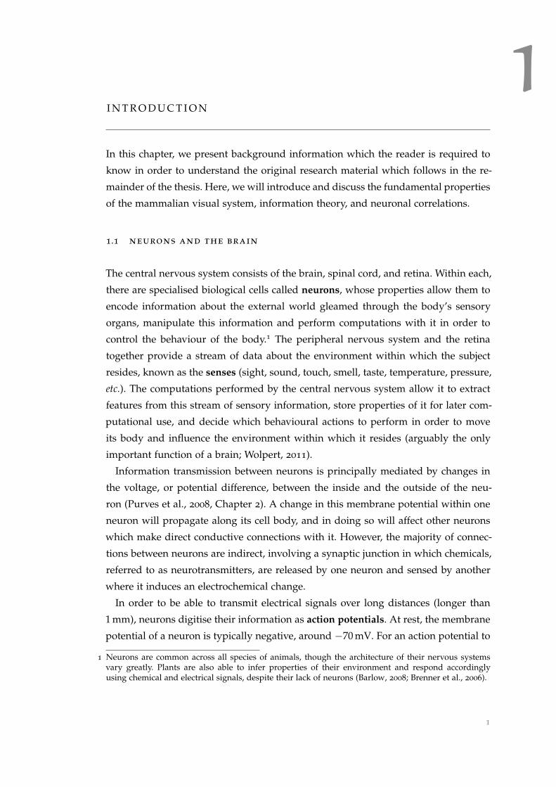


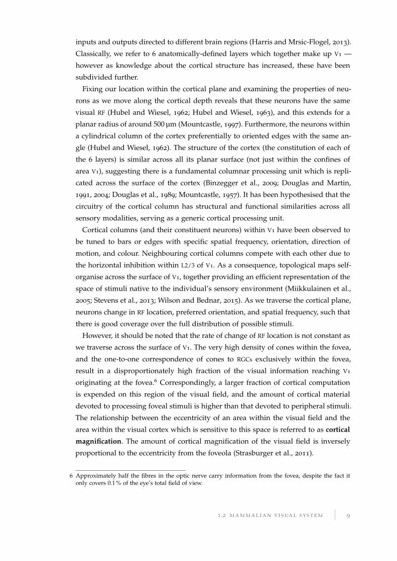
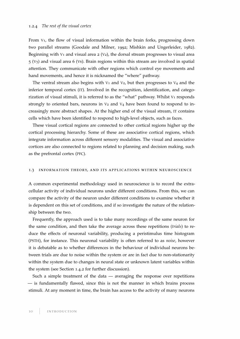
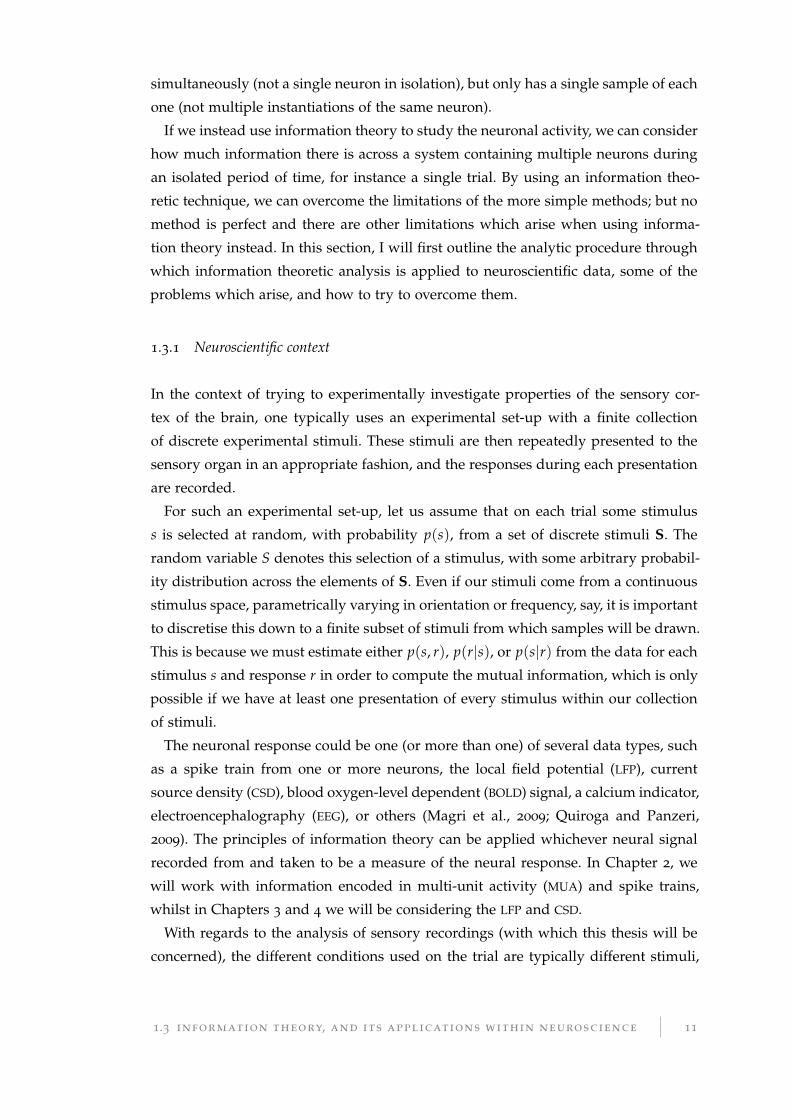
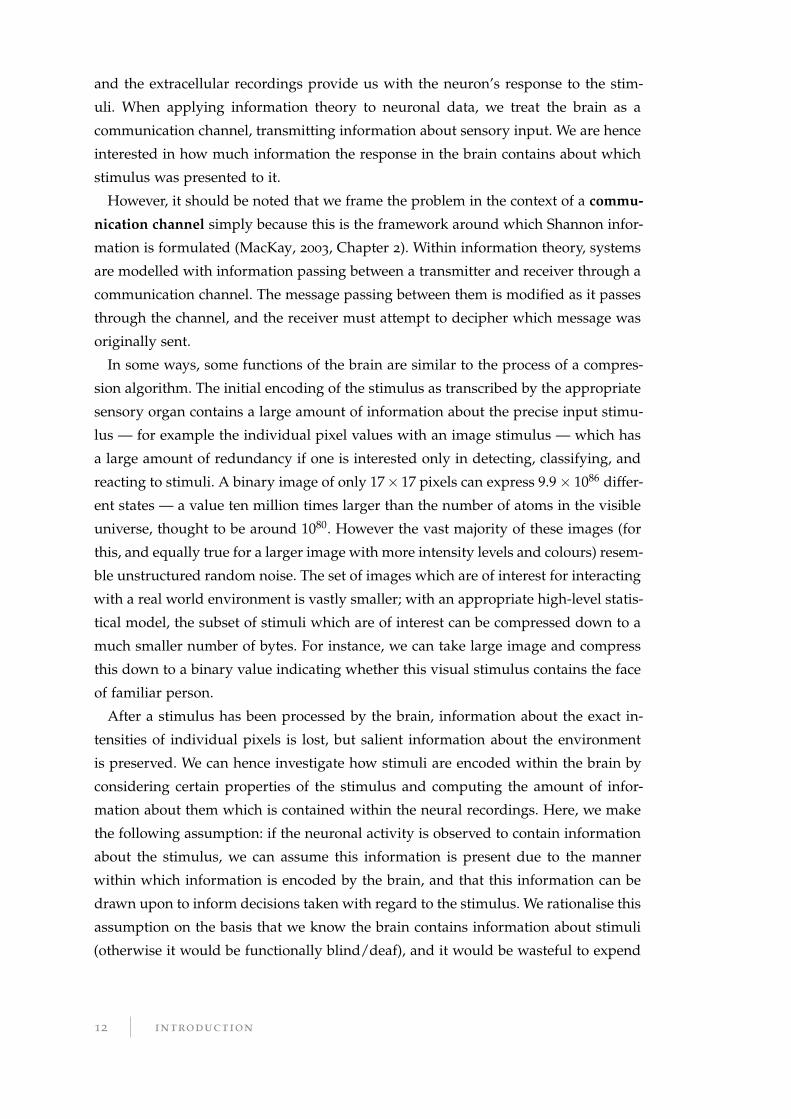


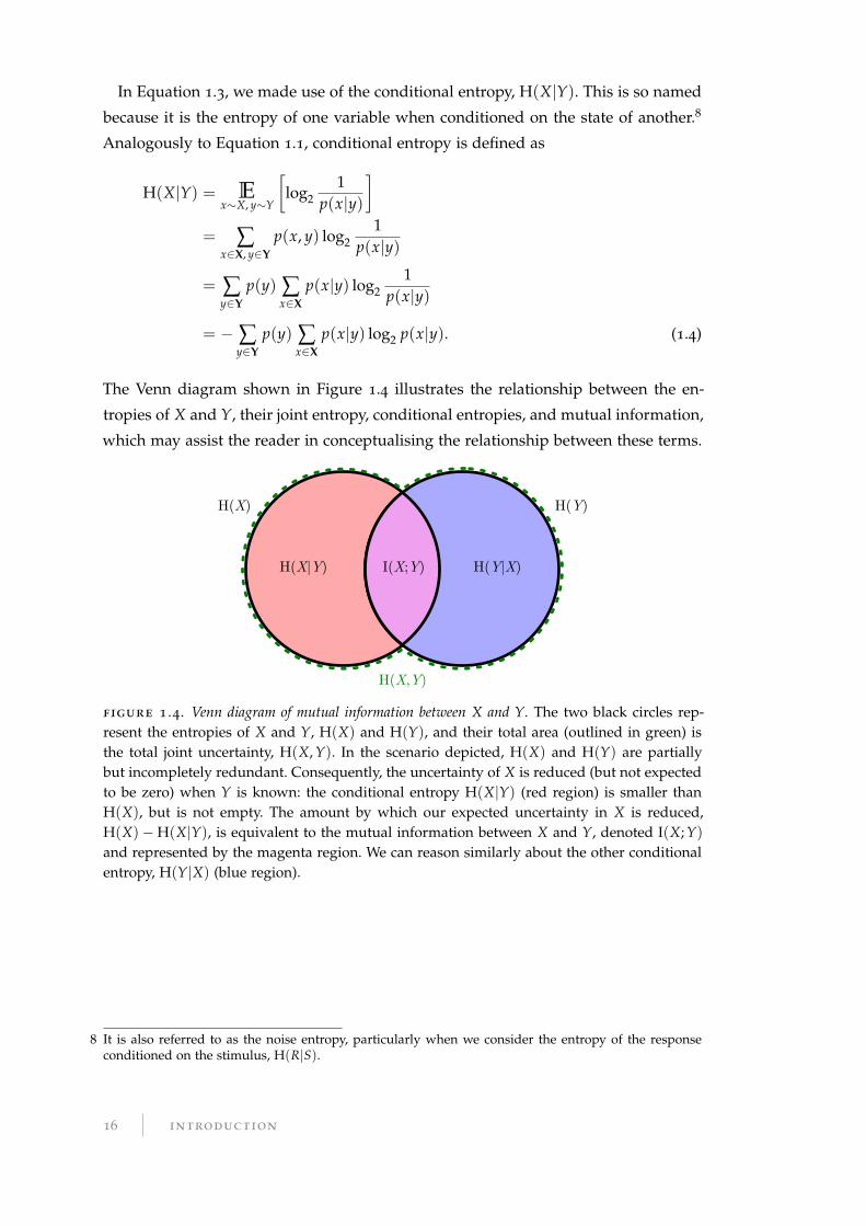
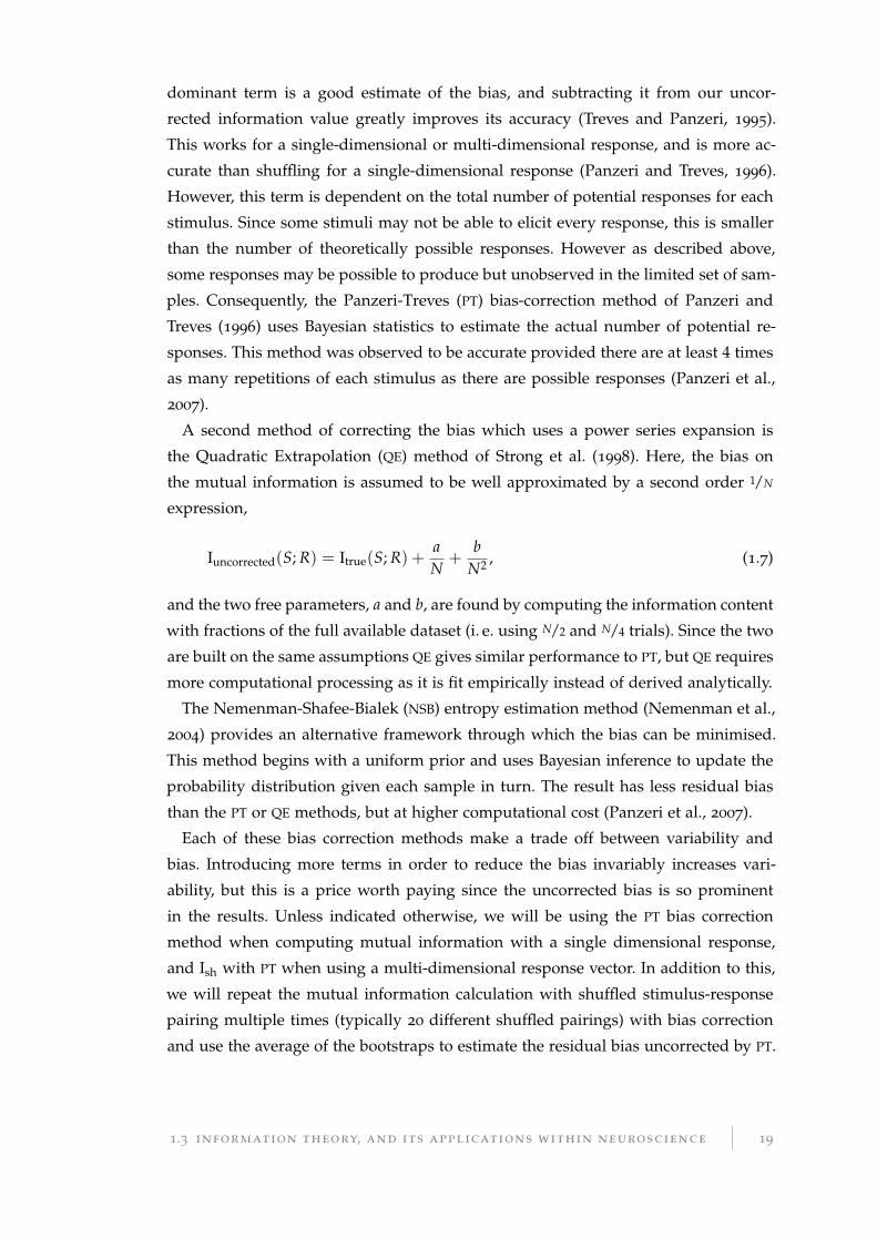

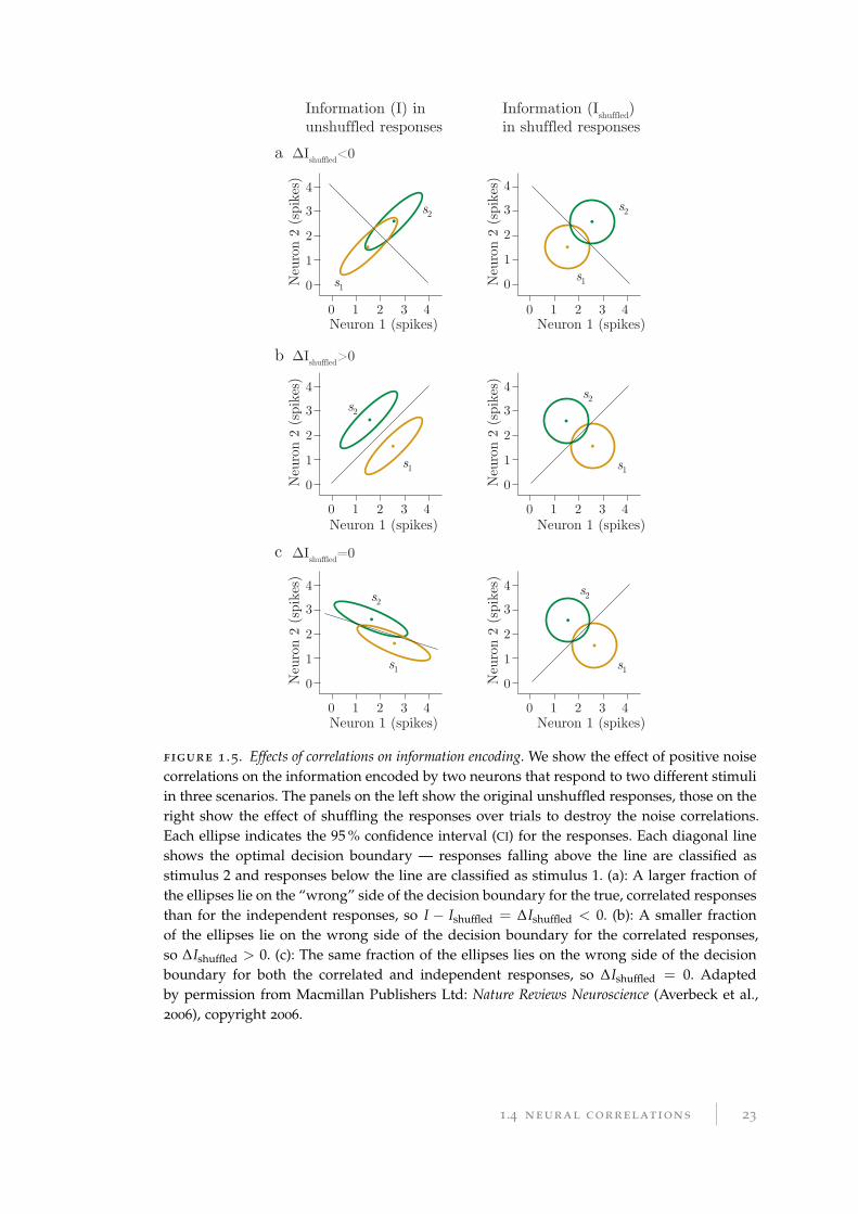


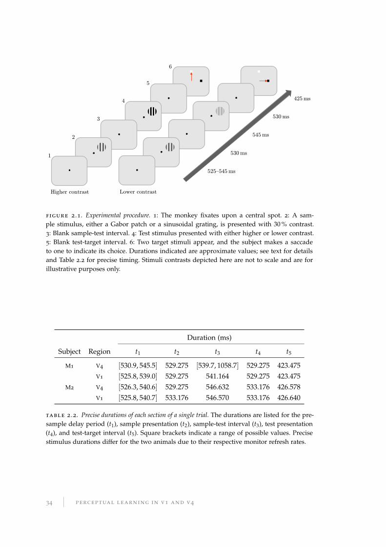

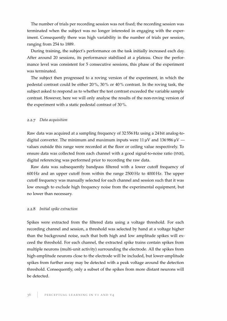
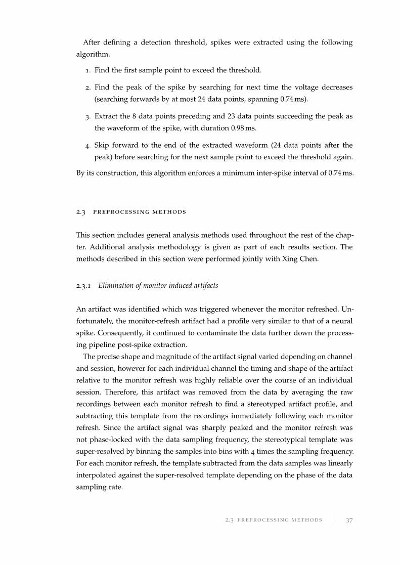


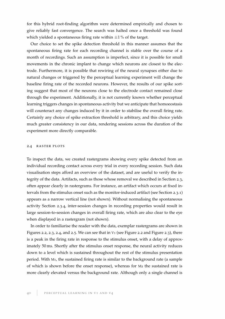
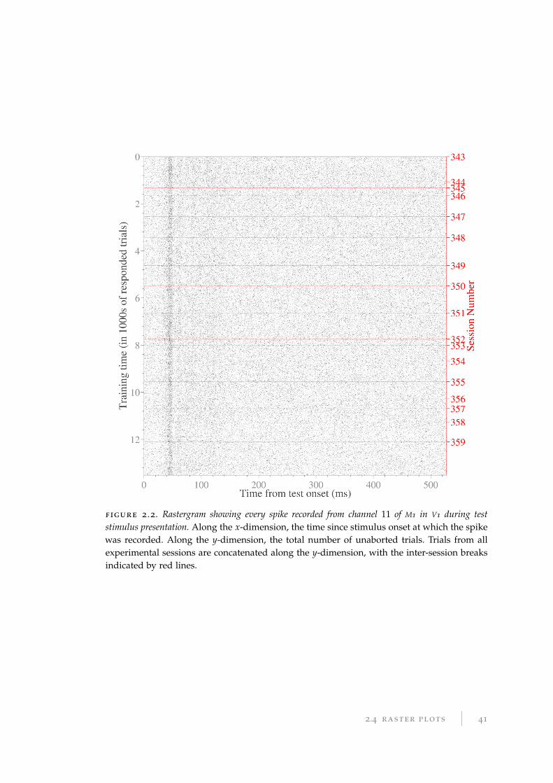


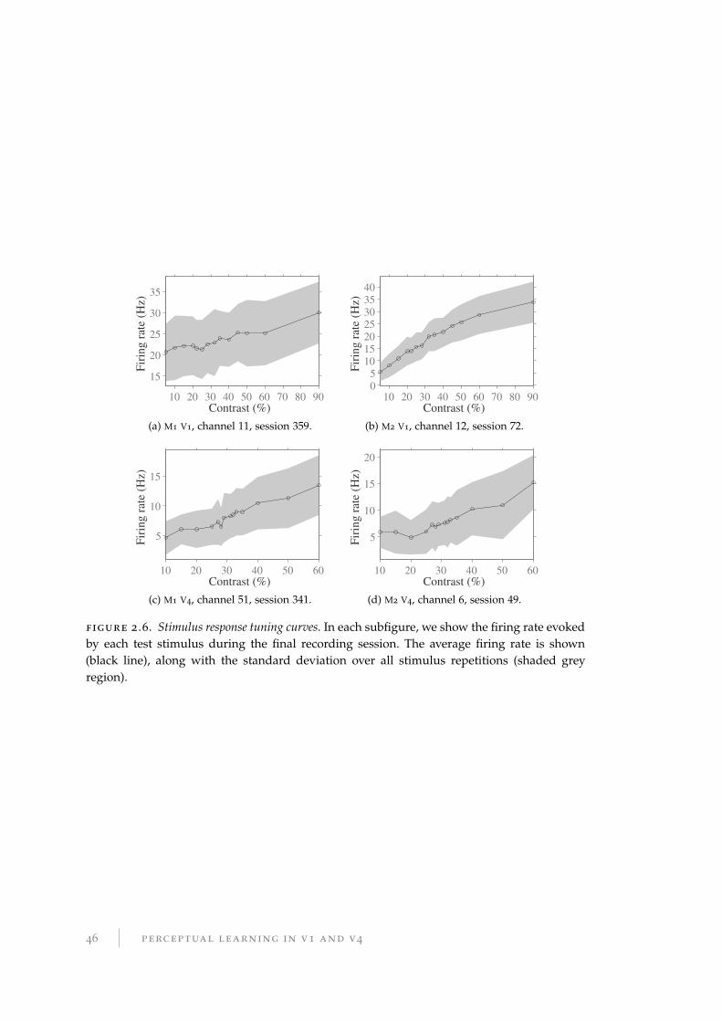
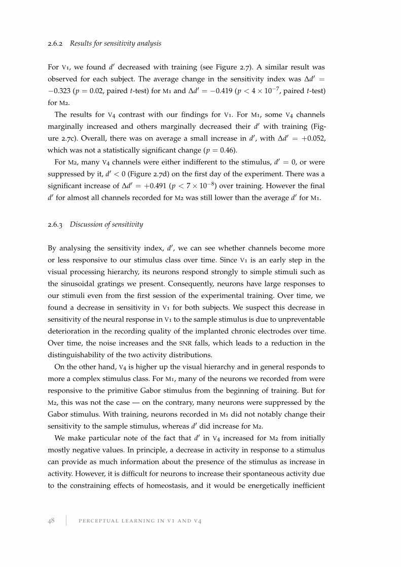

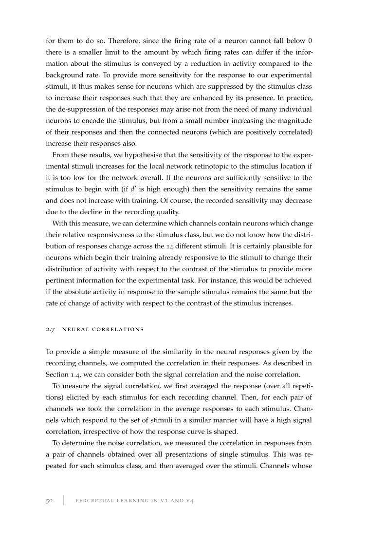

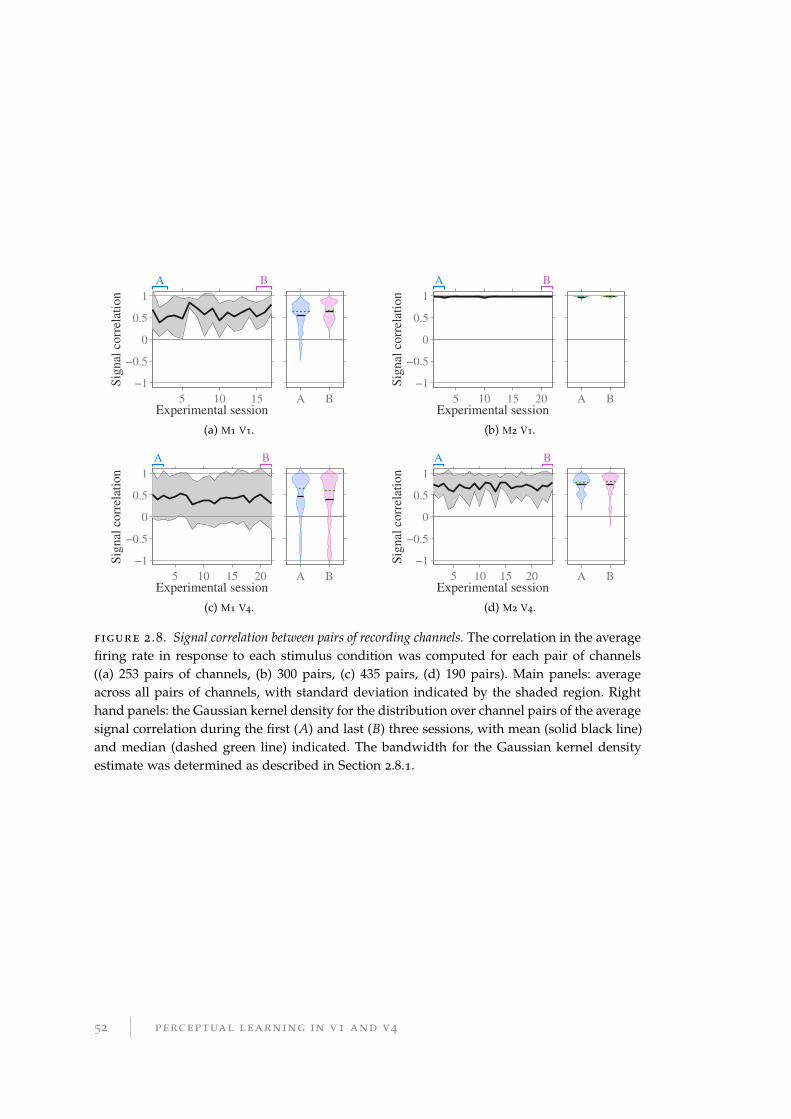
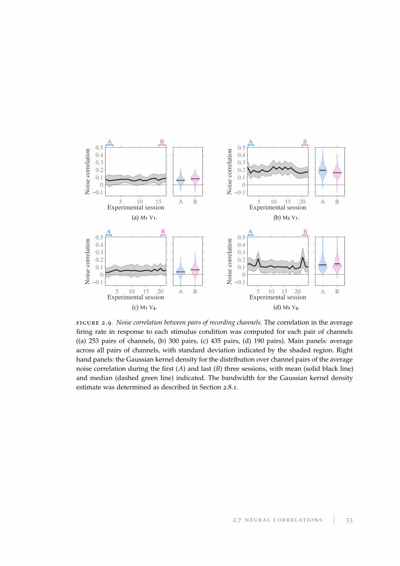

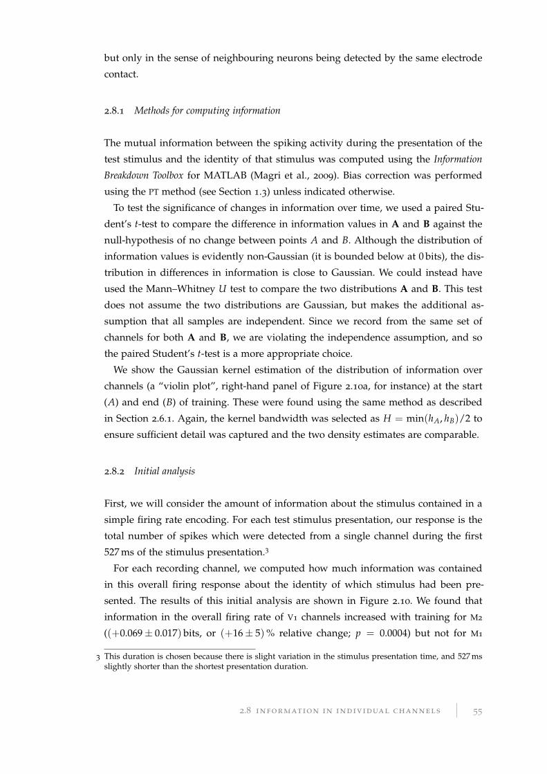

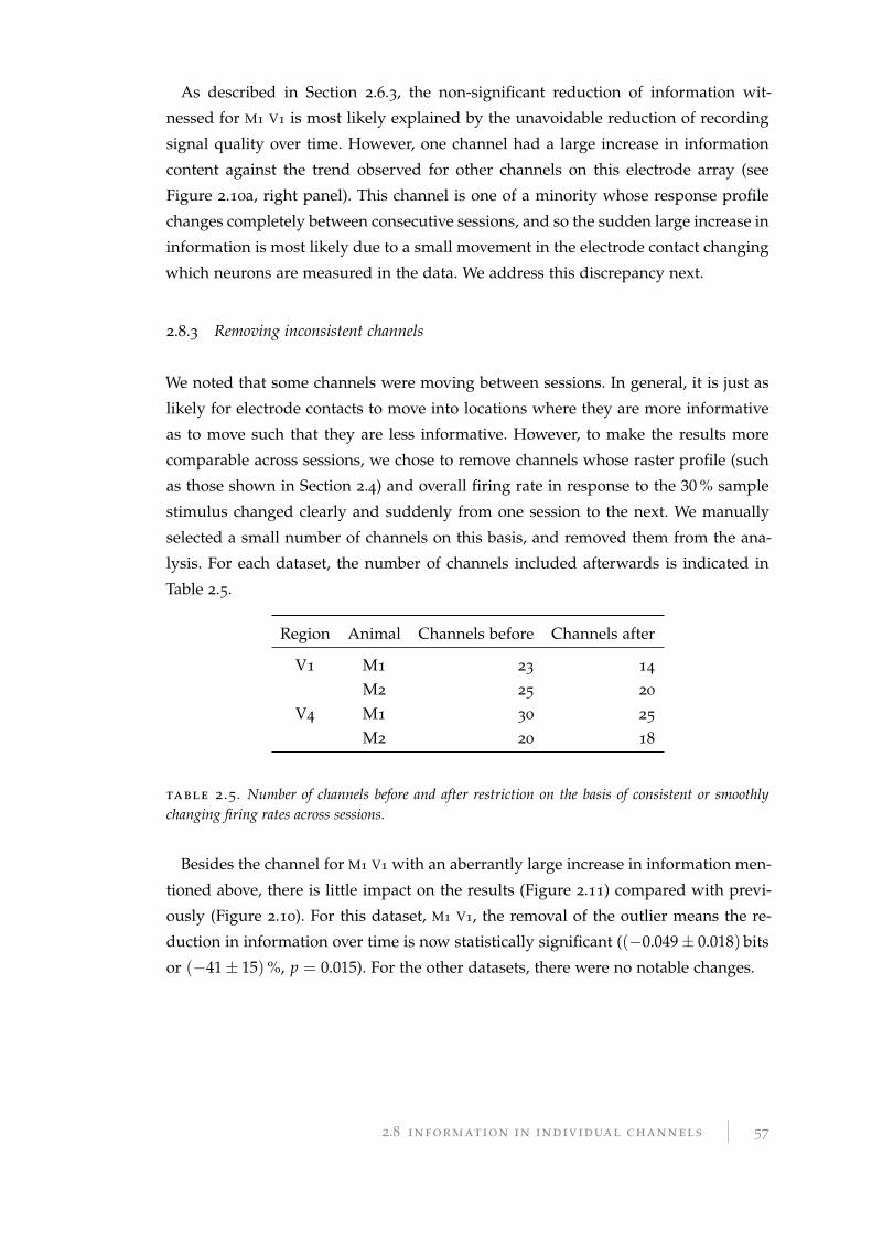
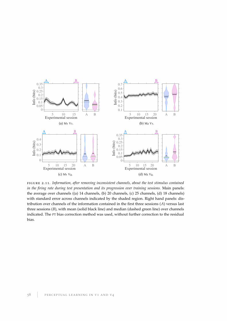


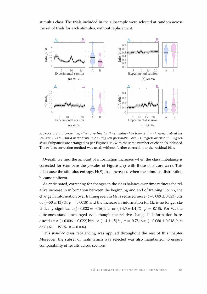
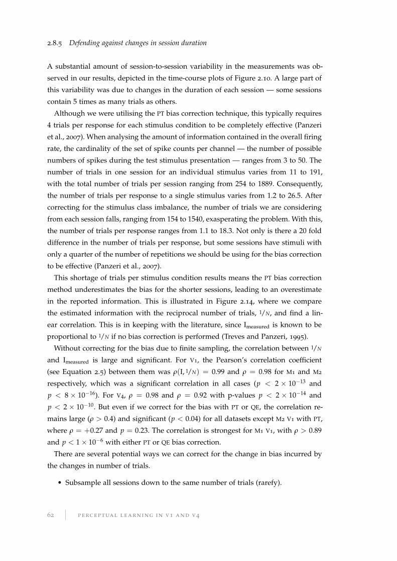
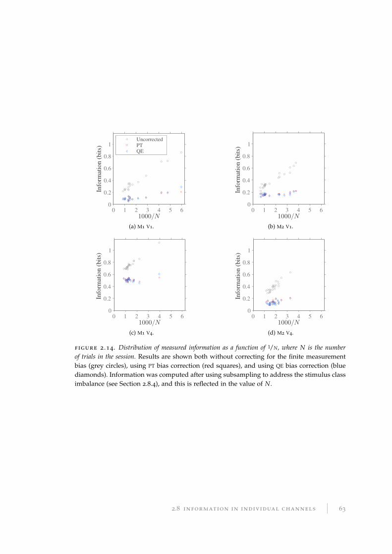
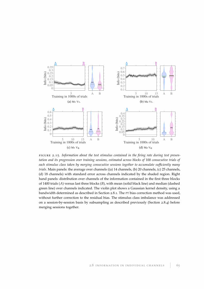


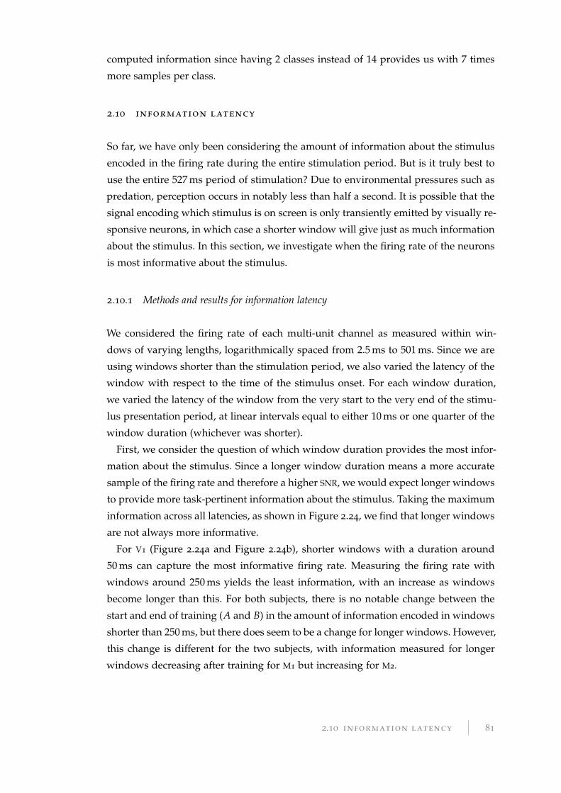
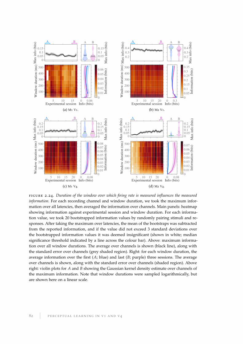
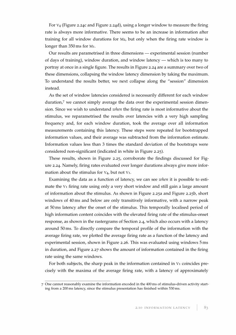

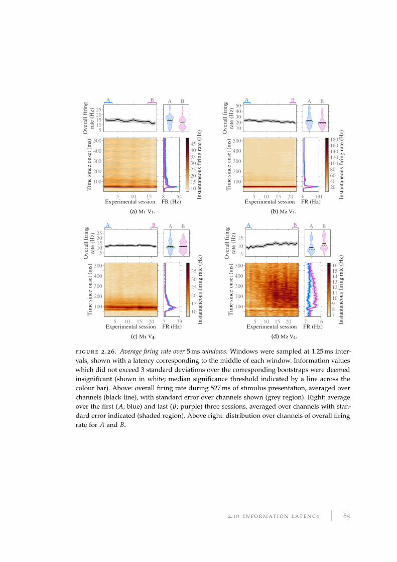

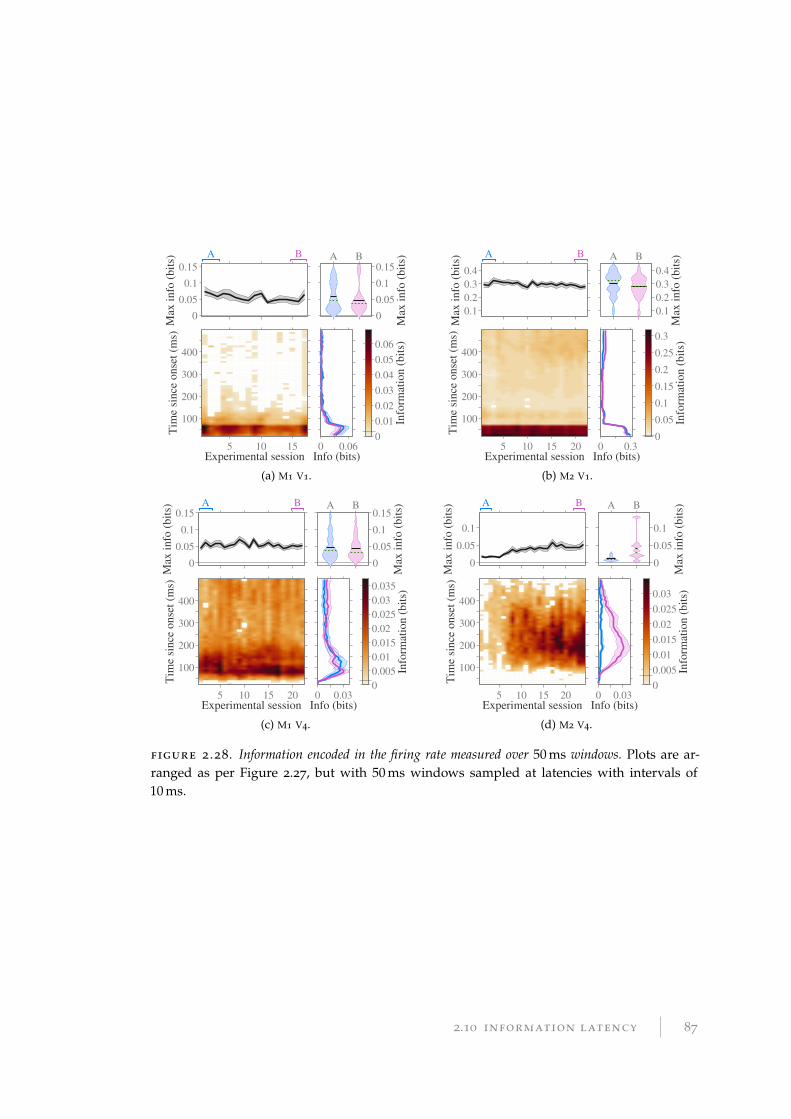
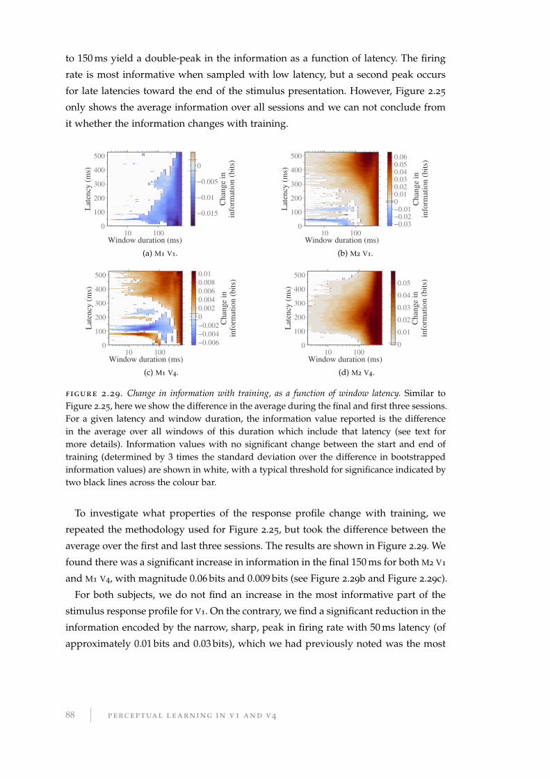


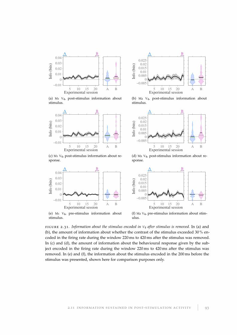

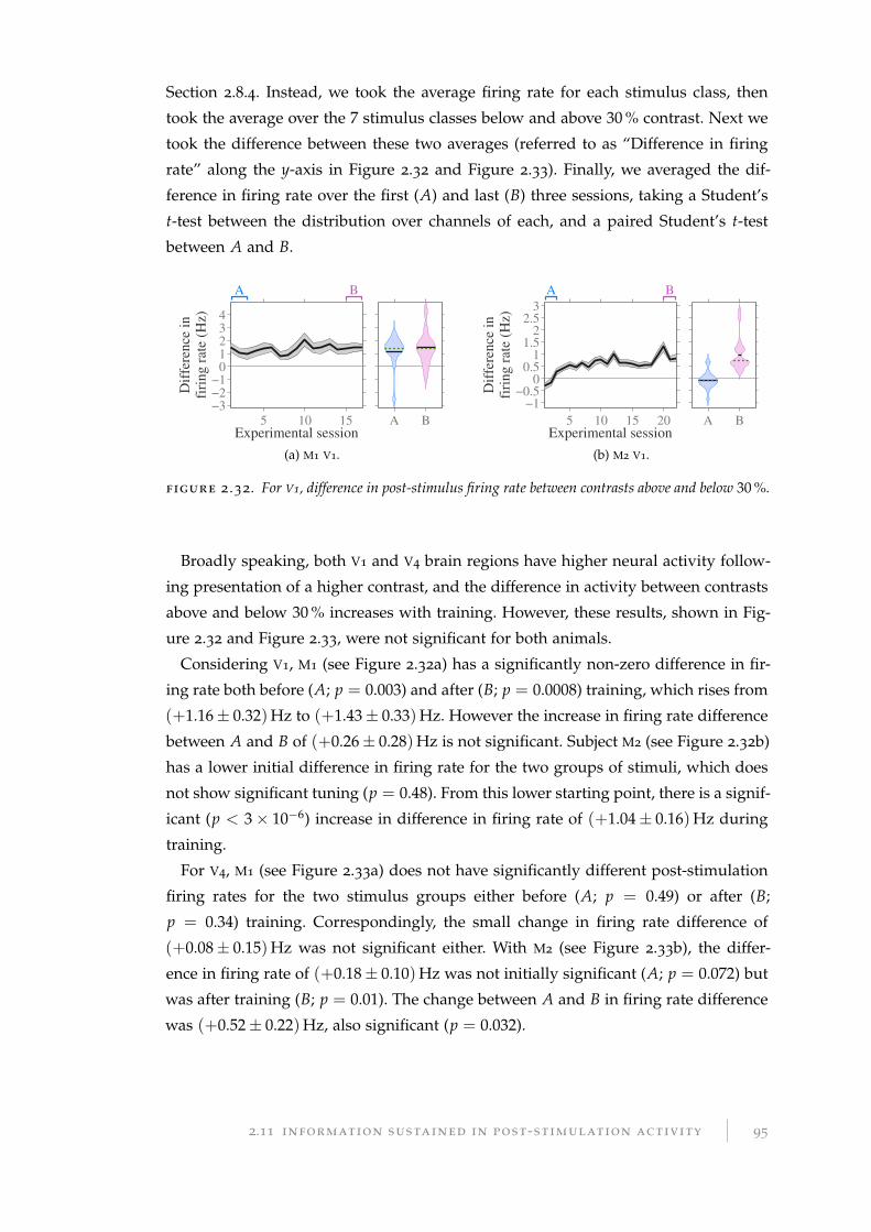
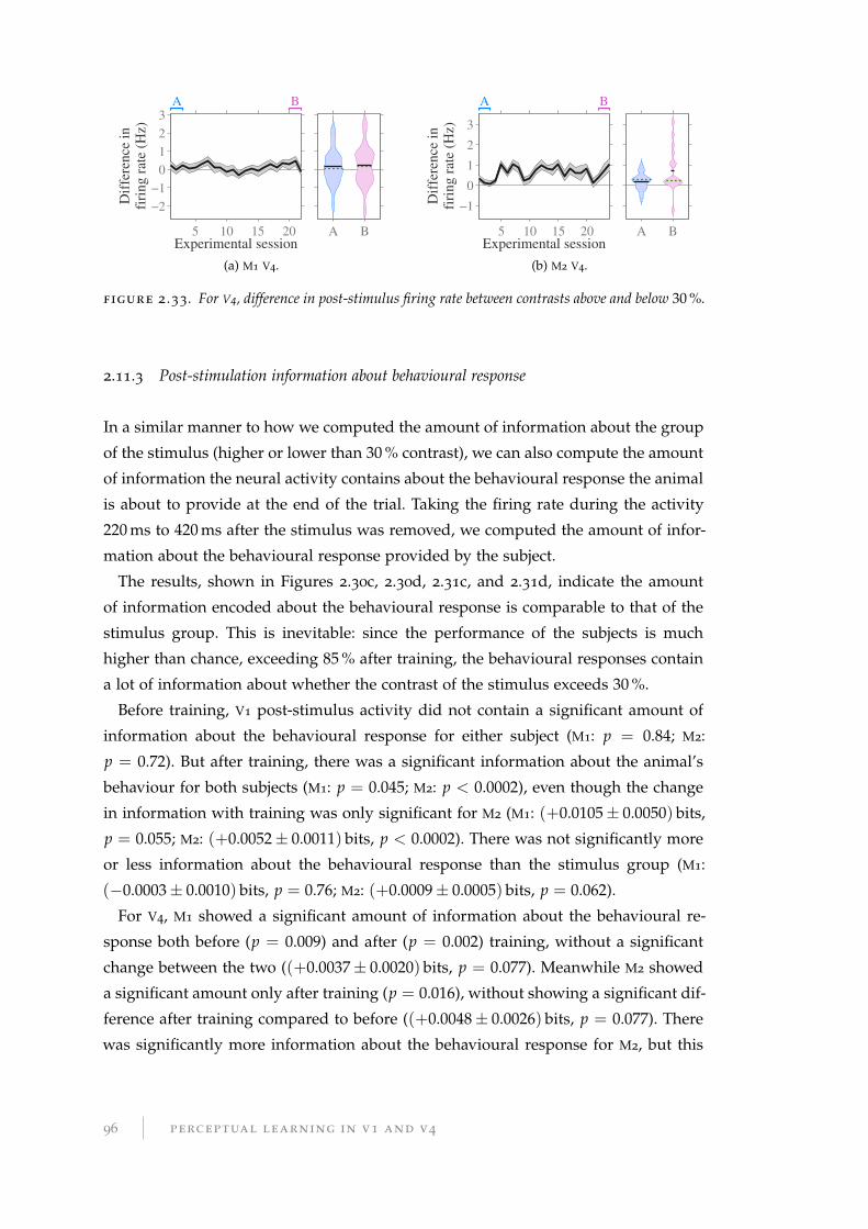


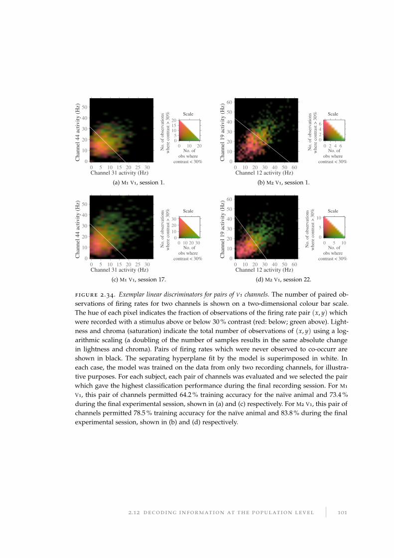
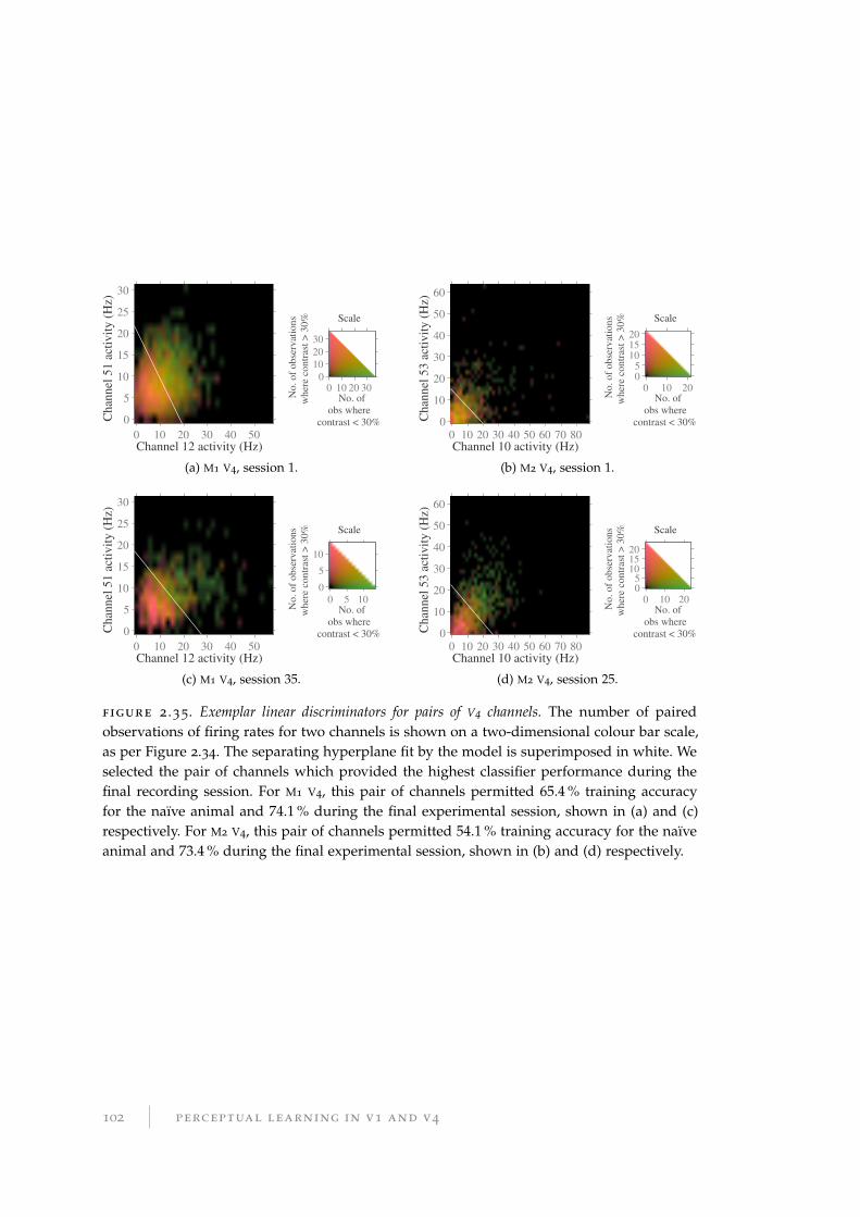


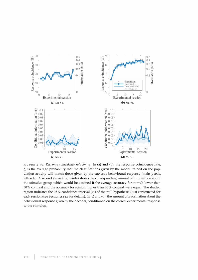


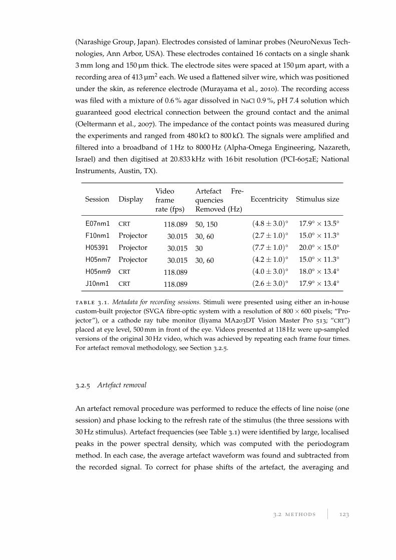

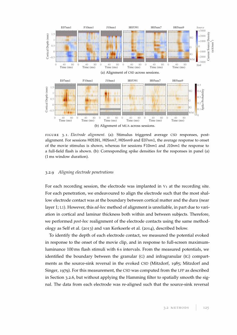
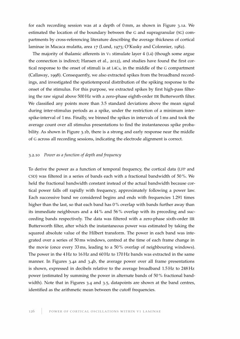


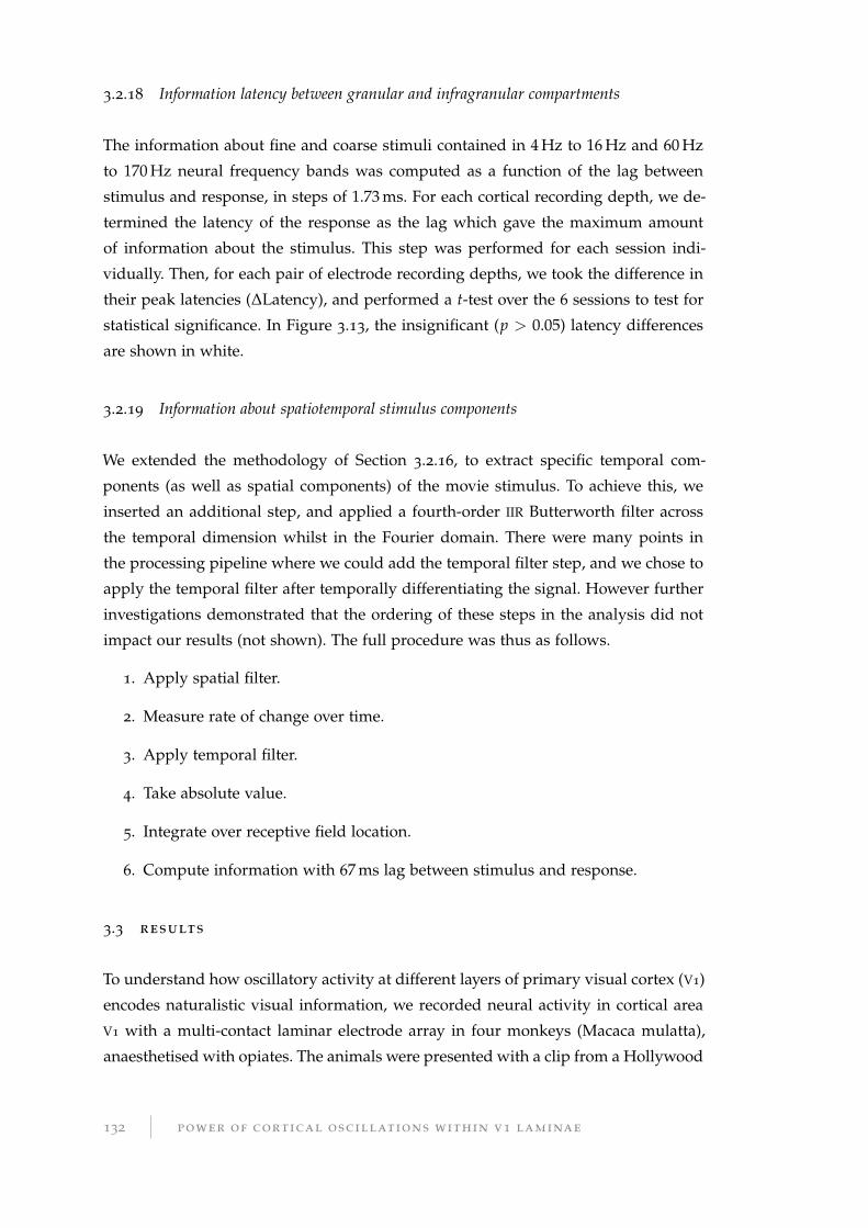
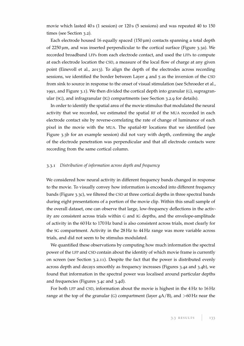
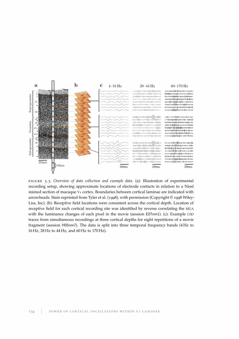
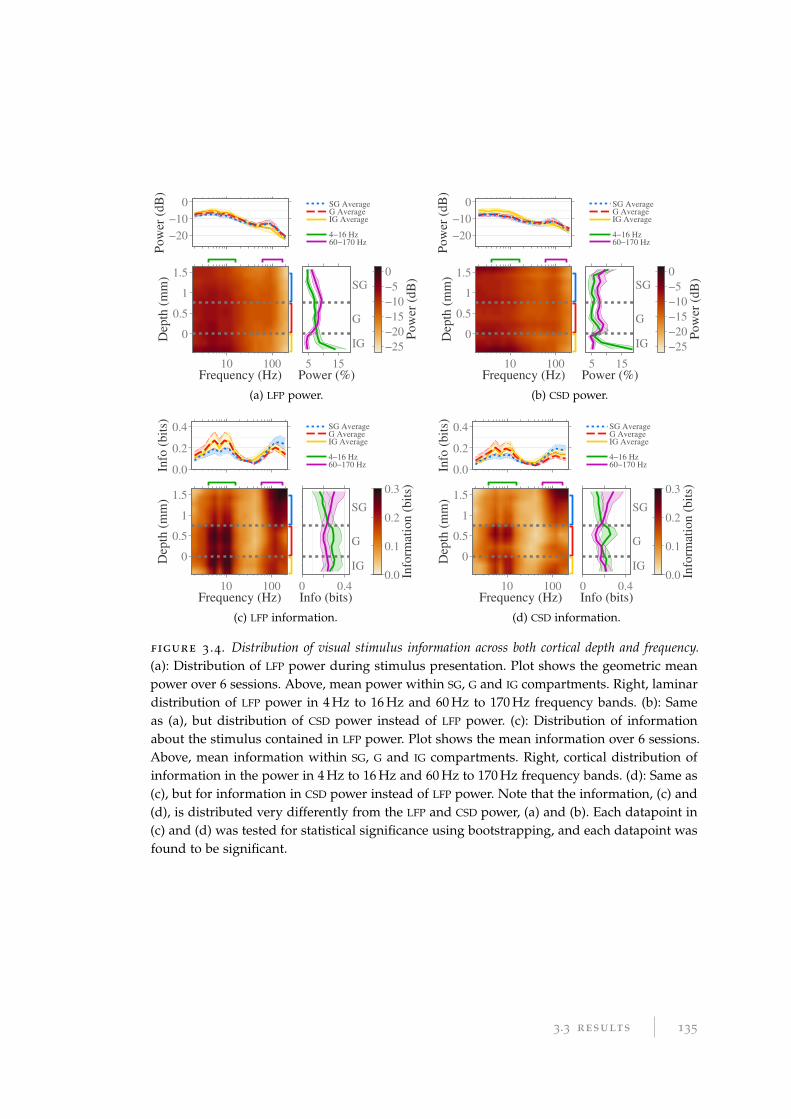
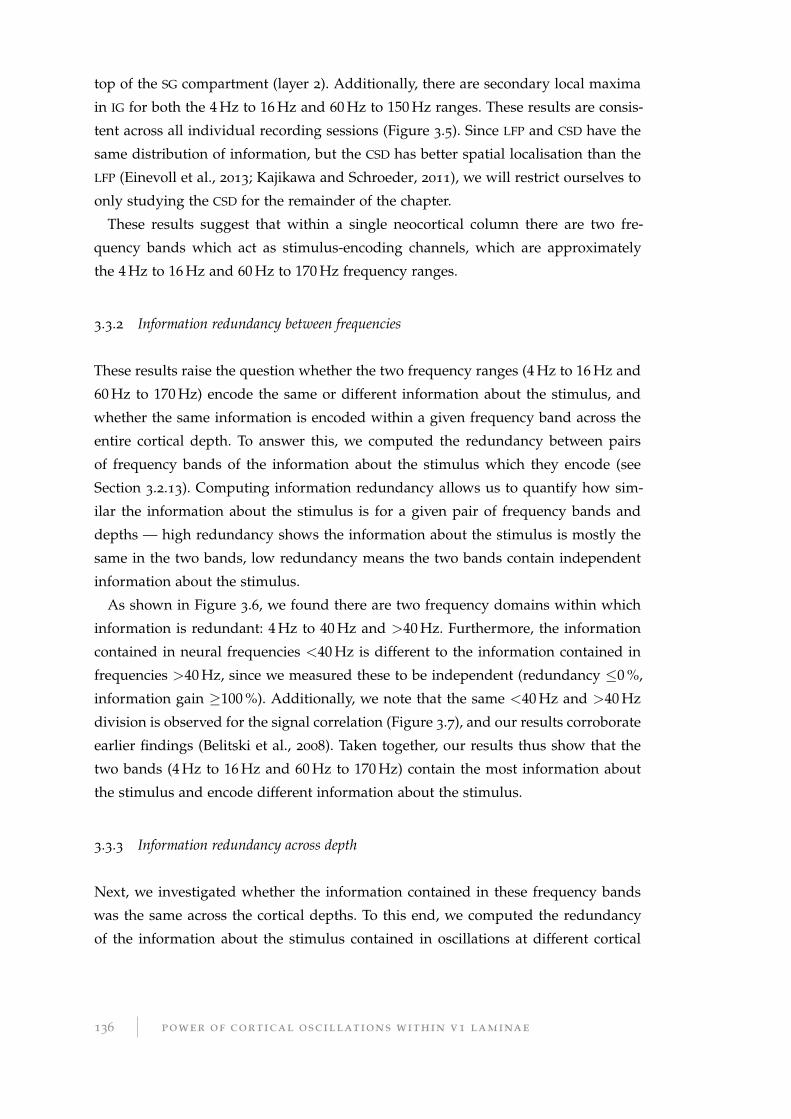

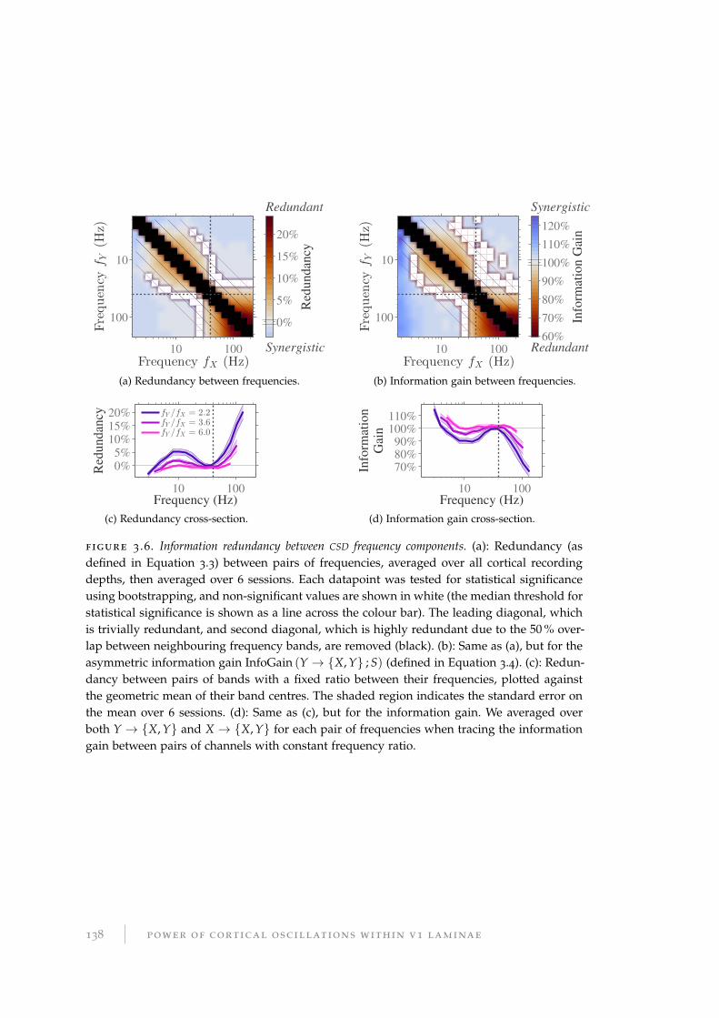


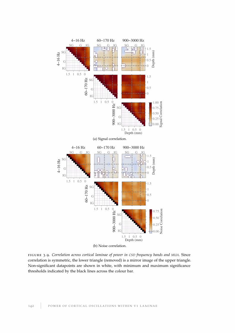


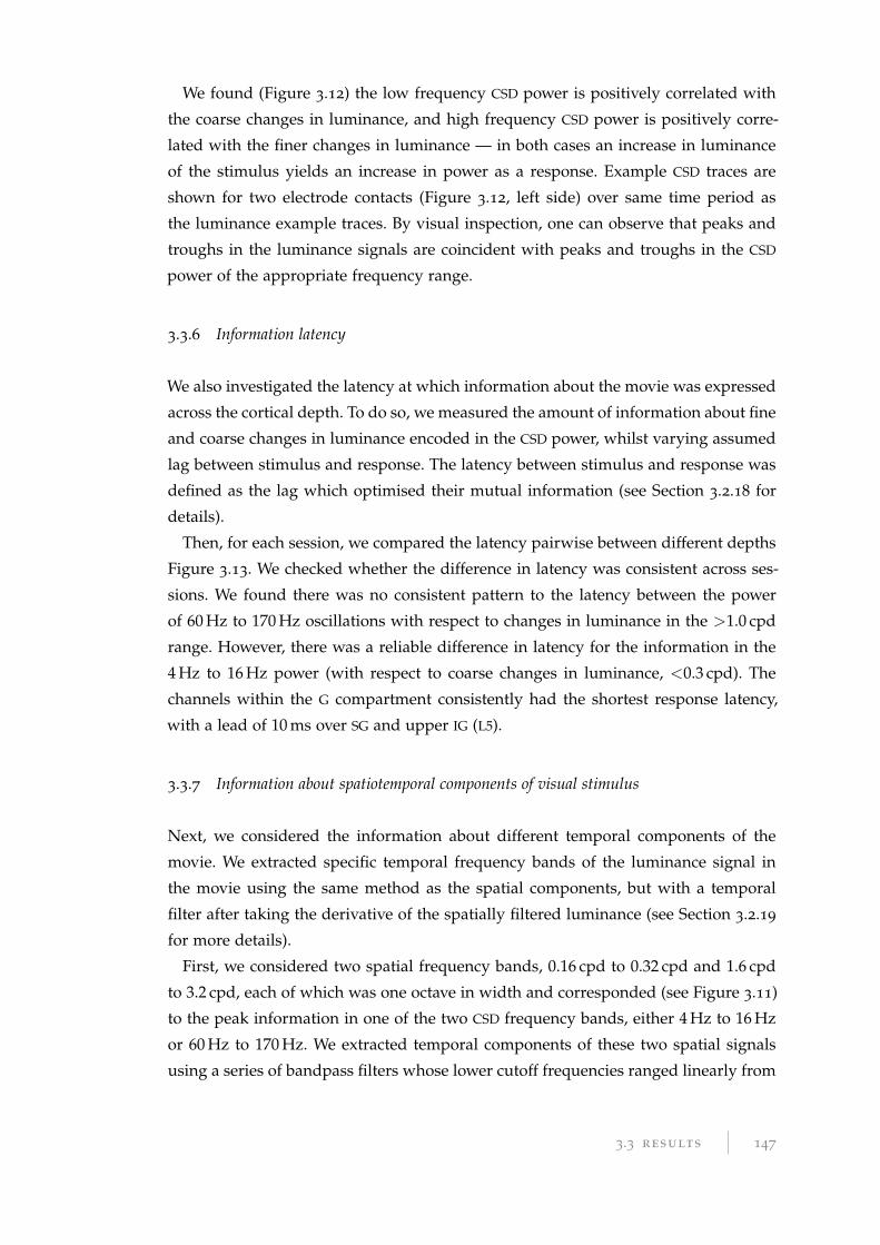
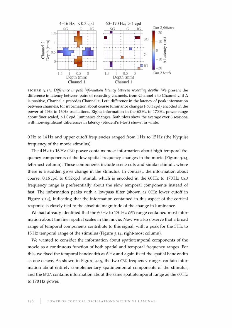
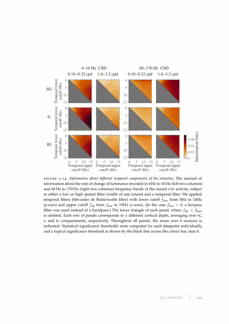
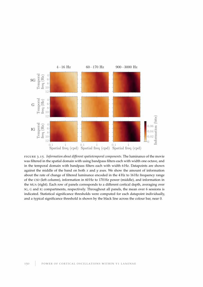


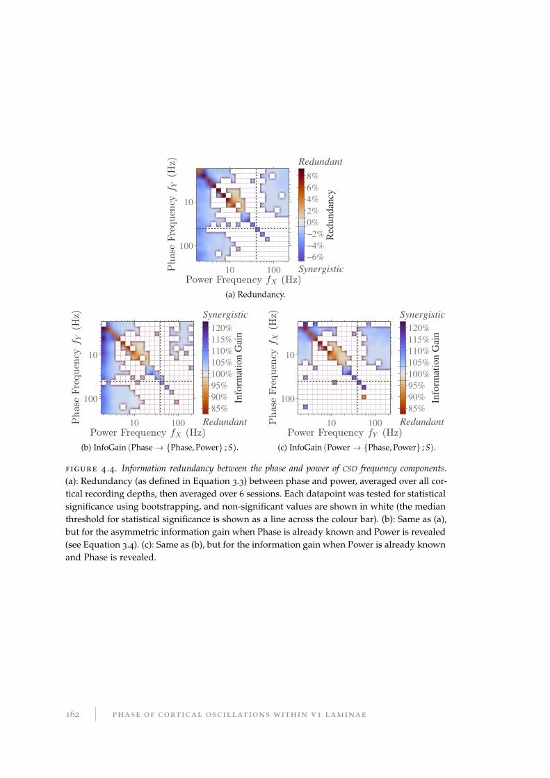
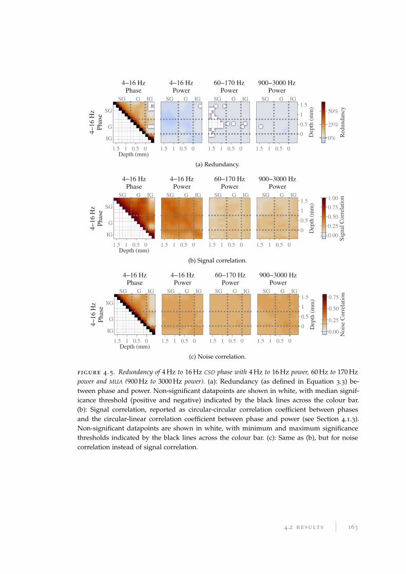
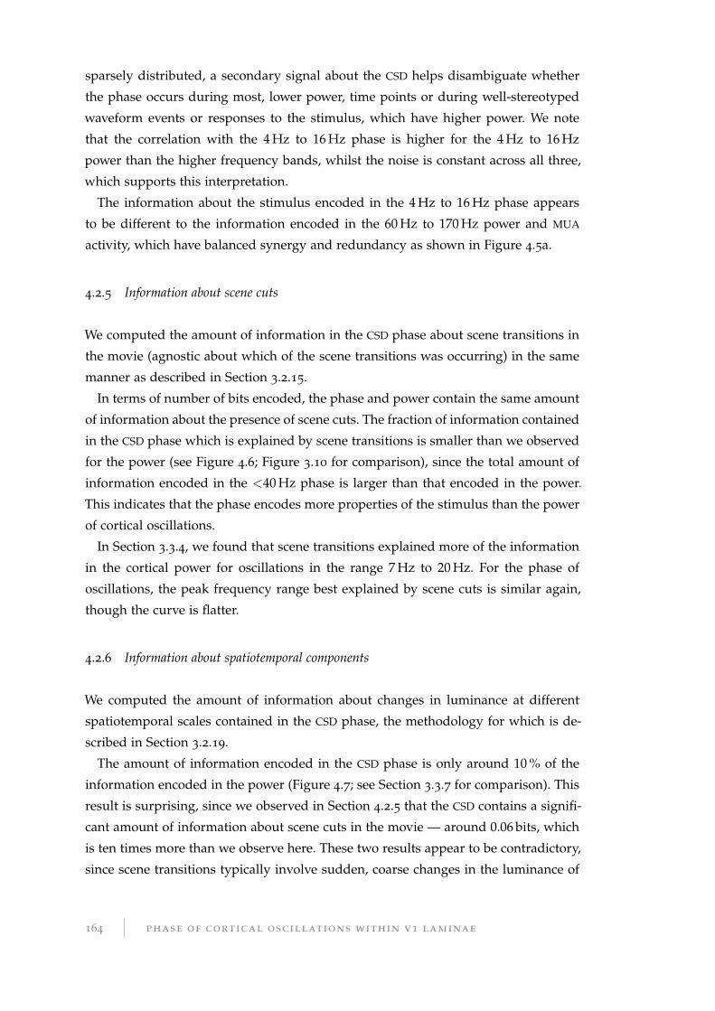
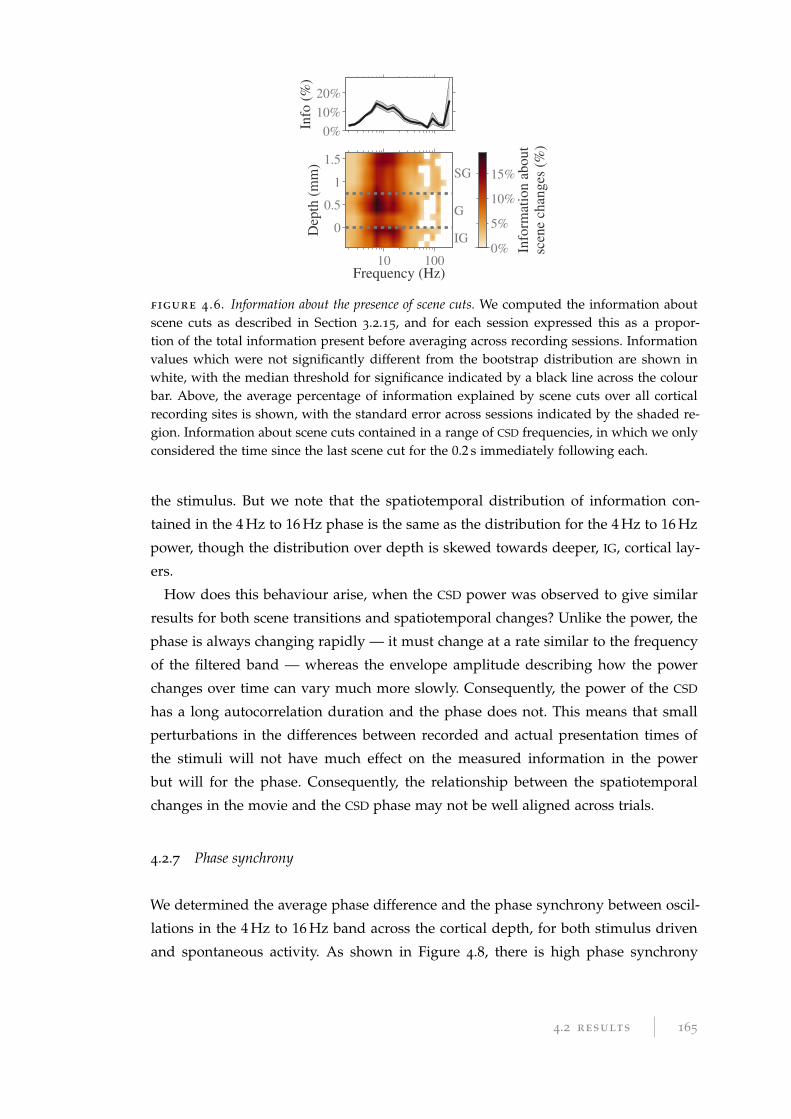
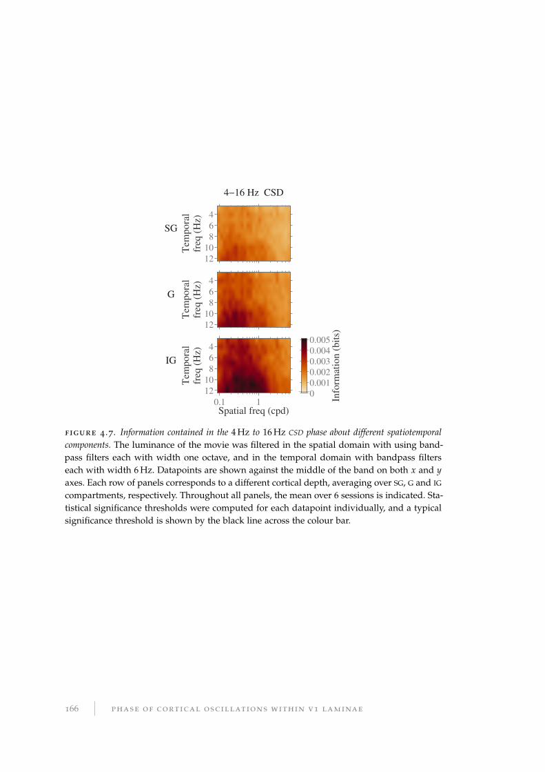
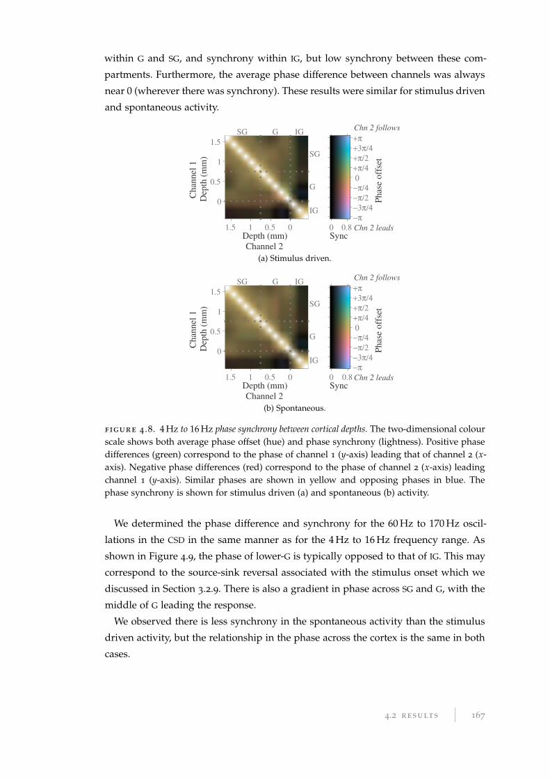
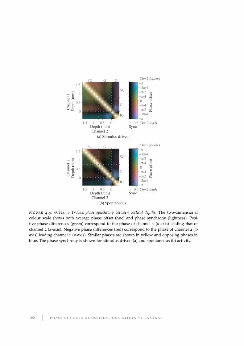
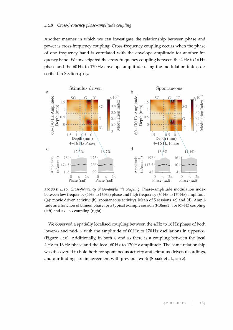


![Association . 5)u]ider, John Lowe & Son viled at Per- 200106.pdf · Association. 5)u]ider, John Lowe & Son viled at Per-ritt Terrace, 13 Perritt Street, Balmain from 1884 to 1909.](https://static.documents.pub/doc/80x56/5f0f728f7e708231d4443559/association-5uider-john-lowe-son-viled-at-per-200106pdf-association.jpg)


