Revisions: 2013 June – 2014 October: David Bailey <[email protected]> 2006 October: Jason Harlow
with suggestions from John Shepherd 1997: Joe Vise 1988: John Pitre
Please send any corrections, comments, or suggestions to the professor currently supervising this experiment, the author of the most recent revision above, or the Advanced Physics Lab Coordinator.
INTRODUCTION Nuclear Magnetic Resonance (NMR) occurs when photons are resonantly absorbed and
emitted by transitions between different energy levels of a nucleus in a magnetic field. NMR has applications ranging from fundamental physics to oil prospecting, and from quantum computers to medical imaging. NMR related Nobel Prizes include Rabi (1944), Bloch & Purcell (1952), Ernst (1991), Wüthrich (2002), and Lauterbur & Mansfield (2003).
The goals of this experiment are to explore basic NMR methods, measure the magnetic moment of the proton, and to use NMR to probe the environment of the protons in materials.
Theory Many nuclei have a non-zero spin angular momentum, I
, and consequently a nuclear
dipole moment, µ
. For a particle of mass m and charge q, we can write
µ= γ I= g q
2mI
(1)
where γ is the gyromagnetic ratio, and g is the “g-factor”. A classical rotating object of any shape has g=1 as long as its charge and mass have the same distribution. For a spin ½ quantum point particle, g=2 (plus small corrections).
The interaction of magnetic dipoles with a static magnetic field gives rise to a series of energy levels. The energy differences are small, typically corresponding to radio frequencies (e.g. 42.58 MHz for protons in a 1 Tesla magnetic field), and an appropriate r.f. (radio frequency) field will induce magnetic dipole transitions between the different states.
Resonance Condition The interaction energy of a magnetic moment, µ
with a constant external magnetic B
o is
E = −µ⋅Bo = −γ I
⋅Bo (2)
This experiment studies hydrogen nuclei (protons) which have spin I = ½, so in a magnetic field Bo = B0 z , their spin z eigenstates can be written ↑p and ↓p , and their eigen energies are
E↑ = 12 γBo and E↓ = − 1
2 γBo (3)
Photons can be resonantly absorbed or emitted when their energy, hν0, is equal to the energy difference between the two levels, i.e. hvo = ΔE = γBo (4) The corresponding angular frequency ωo =ν0 2π = γBo is known as the Larmor frequency. It can also be derived classically as the frequency of precession around the z axis of a spinning ball with magnetic moment µ
= γ I
in an external field, B0 = Boz .1
Transitions The spontaneous emission rate for a magnetic dipole transition to a lower energy state is2
1 See Abragam, p19, or p283 of “Mechanics”, K.R. Symon, 2nd Ed., Addison-Wesley, 1971. (QC 125 S98 1961) 2 SI version of “Spontaneous Emission Probabilities at Radio Frequencies”, E. M. Purcell, Phys. Rev. 69 (1946) 681.
This depends on the third power of the frequency, and at radio frequencies is too small to be significant. For example, an isolated proton in a 0.75T magnetic field has a spontaneous emission lifetime of 2×10¹⁷ years3 – longer than the age of the universe.
Protons in NMR samples are, however, not isolated.4 They are separated by distances much less than the NMR wavelength, so coherent spontaneous radiation increases the emission rate by hν/kT. 5 The protons are also enclosed in a coil which provides a further enhancement of Qλ3/V, where Q is the quality factor of the coil’s resonant circuit, λ is the NMR wavelength, and V is the volume. For protons in a 0.75T magnetic field at room temperature in a sample coil with Q=100 and V=1cm3, the total emission rate is ~10-10/s.
A 1 milliwatt, 30 MHz generator can produce about 1022 photons per second in the resonant range Δν. If these photons are spread over a ~1 cm2 area (as for our apparatus), then ρν=1022 h/c photons/cm2/s, and the rate for stimulated absorption (or emission) for protons in a0.75T magnetic field is6
ρνB21 = ρνc3
8πhν 3A21 = ρν
2π 2c2µ 2
3ε0h2 ≈1×10⁻⁶ / s (6)
Since the stimulated absorption rate is much higher than the coherent spontaneous radiation rate, such an r.f. field can pump the protons into a non-equilibrium energy distribution.
Population dynamics Initially, the spin system will be in thermal equilibrium with its surroundings (called the
“Lattice”), so the populations of the nuclear energy levels will be proportional to the Boltzmann factor e−E /kT . At room temperature, the energy difference between the two proton spin levels in a 0.75 Tesla field is only 0.1 µeV, much less than the thermal energy (i.e. kT = 26 meV at T=300K), so the population difference between the two levels is only 5×10⁻⁶. Since the transition probabilities for stimulated emission and absorption are equal, it is these minute inequalities in population that make absorption slightly larger than stimulated emission and lead to a net absorption of energy by the spin system when subjected to an r.f. field.
This net absorption of r.f. energy will tend to equalize the populations of the different energy levels. Simultaneously, various relaxation mechanisms tend to maintain thermal equilibrium by the exchange of energy between the spin system and the lattice. For example, in water the protons are part of H2O molecules or H+ or OH– ions, all of which are subject to Brownian motion. The local magnetic field at any point is the sum of the external magnetic field plus the rapidly fluctuating magnetic fields of all the neighbouring nuclear and electronic magnetic moments. Any Fourier component of this fluctuating field at the resonant frequency ν0 will induce transitions between the nuclear magnetic energy levels. This process provides a
3 Abragam, p. 264-65. There is a factor of two due to the two possible polarizations of the emitted photon. 4 This is the standard description of NMR, but not everyone agrees; see “The Origins and Present Status of the Radio
Wave Controversy in NMR”, D.I. Hoult, Concepts in Magnetic Resonance 34A (July 2009), 193-216. 5 “Coherence in Spontaneous Radiation Processes”, R.H. Dicke, Physical Review 93 (1954) 99–110. 6 See Chapter 1 of “Spectra of Atoms and Molecules”, Peter F. Bernath, Oxford 2005, 2nd Edition,. There are multiple
ways to define these Einstein A and B Coefficients in the literature, so it easy to get confused.
relaxation mechanism by which energy can be exchanged between the spin system and the translational and rotational degrees of freedom of the molecules and ions.
In this experiment, relaxation mechanisms are studied by measuring the recovery of the magnetization after it has been disturbed by a pulse of r.f. power at the resonant frequency. In thermal equilibrium before an r.f. pulse is applied, the protons have a longitudinal magnetization, i.e. the net magnetic moments are aligned with so the net proton spin state can be written spinz
initial = ↑ (7)
The Meaning of π /2 and π pulses An r.f. pulse at the Lamor frequency will induce transitions between ↑ and ↓ states,
producing a mixed state spinz =α ↑ +β ↓ (with α2+β2=1) (8)
A π/2 pulse is an r.f. pulse with an amplitude and duration that will transform an initial ↑ state into the symmetric state
spinzπ /2 =
12
↑ + ↓( ) (9)
Classically, this corresponds to rotating the magnetic moments into the x-y plane, i.e. a 90° or π/2 rotation into transverse magnetization. These classical moments will now precess (rotate direction) in the x-y plane at the Larmor frequency. Ideally, the duration ∆t of a π/2 pulse is related to the r.f. pulse magnetic field (Brf) by the Larmor condition, i.e. ∆t = 4/ν0
rf = 8π/γBrf. Similarly a pulse of the same amplitude but twice as long will reverse the longitudinal
magnetization, i.e. transform an initial ↑ state into a final ↓ state. This is called a π pulse, since classically it corresponds to rotating the magnetic moments by 180°.
After either a π/2 or π pulse, if no further pulses are applied, thermal processes will cause the magnetization to “relax” back to its initial thermal equilibrium state, i.e. the transverse magnetization returns to zero and the longitudinal magnetization returns to its equilibrium value.
The Meaning of the Time Constants T1, T2, and T2*
Most simply, T1 parameterizes how fast a system of spins changes total energy, and T2 parameterizes how fast the spins within the system go out of phase in a perfectly uniform external magnet field
B0 . T2
* includes the effect of inhomogeneities in B0 on the dephasing.
The time constant T1 is defined as the time required for a system of spin magnetic moments to reach thermal equilibrium after an externally applied magnetic field is changed or an r.f. pulse is applied to the system. For example, if a magnetic field is suddenly turned on, the magnetization of an initially unmagnetized system will grow as
M t( ) =
M0 1− e
−t/T1( ) (10)
Similarly, if an r.f. pulse puts a spin system into a non-equilibrium state, it will exponentially decay back to its equilibrium state with the same time constant T1, producing an observable r.f. “free induction tail” (produced by Larmor photons from ↓ ⇒ ↑ transitions).
T1 is known as the “spin-lattice” or the longitudinal relaxation time. Reaching thermal equilibrium in a static field requires the exchange of energy between the spins and their environment, so T1 depends on the mechanisms available for the spins to transfer energy to other
Bo
5
repositories of thermal energy such as the translations, rotations, vibrations, and excitations of the surroundings, collectively called the lattice. We assume that the spin system has a very small heat capacity so that the spin energy cannot disturb the lattice temperature.
T2, known as the “spin-spin” or the transverse relaxation time, is the time over which spins in a system move out of phase with each other due to “static” internal magnetic inhomogeneities. (“static” may include fields changing slowly compared to T1.) Such phase coherence changes can occur without any energy being lost or gained by the spin system. T2 is meaningless if there is no net polarization, so T2≤T1.
T2* is the time constant that describes the decay phase coherence when magnetic
inhomogeneities are included. For example, immediately after the application of a π/2 pulse, all the magnetic moments are aligned, but if there are inhomogeneities in the static magnetic field over the sample then different magnetic moments will precess at different rates, shortening the transverse relaxation time. The exponential shape of the free induction tail depends on T2
* which is always smaller than T2. One can get around the effects of field inhomogeneities and measure T2 directly using the spin-echo technique described later.
An important contribution to T2 is from dipole-dipole interactions causing “spin-spin” relaxation. Each nuclear dipole sees not only the applied static field B
o , but also a small local
magnetic field Blocal produced by neighbouring nuclear dipoles. Since the nuclei are in random
motion, the total magnetic fields Bo +Blocal vary randomly from nucleus to nucleus, so their
precessional frequencies also vary, similar to the effect of inhomogeneities in the static field mentioned above. Since all protons are identical, protons in different local magnetic fields can also quantum mechanically exchange spin states, causing additional local decoherence.
Now consider systems in which not all nuclei are identical, e.g. if paramagnetic ions are added. The spin-exchange process is absent for non-identical nuclei, but the local field effect is present. Since the magnetic fields of Fe+++ ions are ~1000 times greater than the fields of protons, T2 is determined entirely by the Fe+++ ions for the ionic concentrations used in this experiment.
The Equality of T1 and T2 in Liquids Usually T1 >> T2 in solids, but T1 ≈ T2 in non-viscous liquids. The reason for this equality
can be seen if we examine the processes that lead to T1 and T2. Nuclear spin states change when they are stimulated to absorb or emit energy, with a rate
that depends on the intensity of the fluctuations at the resonant frequency ωo. Dipole-dipole interactions can also exchange energy at frequencies ωo (e.g. for an up-up to up-down transition) or 2ωo (e.g. for an up-up to down-down). Whenever a spin changes state, both the energy and phase can change, so both T1 and T2 are affected,
T2 is also sensitive to phase decoherence when spins are in different “static” magnetic fields, corresponding to “zero” frequency fluctuations. The average time it takes for local fields to change by an amount comparable to their magnitude is parameterized by a correlation time τc. In solids, the correlation time is very long since things move little. If two protons are in different magnetic fields, they stay in different fields and quickly move out of phase. Hence T2 is small.
The situation is very different in a non-viscous liquid. The motions of the ions and the fluctuating fields that they create are both rapid and isotropic. For random Brownian motion of
6
spherical ions, the correlation time will be given by7
τ c =4πηa3
3kT=2a2
9D (11)
where η is the liquid’s viscosity, a is the radius of an ion, k is the Boltzmann constant, and T is temperature; the correlation time is related to the Stokes Law diffusion constant D=kT/6πηa. In this simple case, the correlation time also parameterizes the frequency distribution of the local electromagnetic field fluctuations. The contribution to the “static” field variations goes down as the number of fluctuations per precession cycle goes up, i.e. the fluctuations “average out”. The number of fluctuations while a spin precesses once is ~ωoτc, so we expect their average contribution to the “static” field to be negligible if τc << 1/ωo. For a non-viscous liquid at room temperature, collision frequencies are of the order of 1013 Hz and Larmor frequencies are typically of the order of 107 Hz, so this this condition is satisfied and we expect T1 ≈ T2. For a liquid composed of a single type of spins, a more rigorous calculation gives8
1T1=320
γ 42
a6µ04π!
"#
$
%&2
I I +1( ) 2τ c1+ ω0τ c( )2
+8τ c
1+ 2ω0τ c( )2!
"##
$
%&& (12)
1T2=320
γ 42
a6µ04π!
"#
$
%&2
I I +1( ) 3τ c +5τ c
1+ ω0τ c( )2+
2τ c1+ 2ω0τ c( )2
!
"##
$
%&& (13)
The 3 terms at the end of eq. 13 are due to fluctuation frequencies ω=0, ωo, and 2ωo respectively.
How to Measure T2 using Spin-Echoes A π/2 pulse generates a transverse magnetization which, because of the Larmor
precession, will induce an observable voltage in a coil with its axis perpendicular to . The magnetization created disappears (relaxes), producing a free induction decay signal with intensity I rf = I0
rf e−t/T2*
(14) The shape of the induction tail can be used to determine the field inhomogeneity (see Question 2), but measuring T2 instead of T2
* requires a different technique. The method of spin-echoes9 reduces the effect of field inhomogeneities. If a π/2 is
followed by a π pulse applied at a time τ later, the π pulse will flip the spins so they start precessing in the opposite direction. Quickly precessing nuclei now find themselves behind the slowly precessing nuclei, but they catch up so that an additional time τ later all the nuclei will come back into phase and produce a signal in the detector coil. This is a spin-echo. The loss in amplitude of the signal is due solely to any irreversible process and will occur at the time rate T2. Repeated π/2, π pulses with different delay times τ can thus be used to measure T2.
Another technique is the Carr-Purcell pulse sequence10 which is a π/2 pulse followed by π pulses at 1τ, 3τ, 5τ, …. Echoes appear at 2τ, 4τ, 6τ, …. All from the original transverse
7 Eq. 47 of Bloembergen. 8 Eq. 33 of “Relaxation Processes in a System of Two Spins”, I. Solomon, Physical Review 99 (1955) 559-565. 9 See Abragam pages 58-63 10 “Effects of Diffusion on Free Precession in Nuclear Magnetic Resonance Experiments”, H.Y. Carr and E.M.
magnetization produced by the first π/2 pulse. The Carr-Purcell method can both save time and automatically correct for the effect of some nuclei diffusing to regions where is different, which shifts their Larmor frequencies so they do not re-phase for an echo. It is possible to produce a Carr-Purcell sequence with our equipment, but you should not use this method unless the height of the echoes is reproducible from pulse sequence to pulse sequence.
How to Measure T1 Two common methods for measuring T1 are the inversion recovery sequence or π - π/2
sequence and the saturation recovery sequence or π/2 - π/2 sequence. In each case, the first pulse prepares the spins and the second pulse measures the magnetization after a waiting period.
π - π /2 (Inversion Recovery) Sequence A π pulse inverts the spin population and thus the magnetization, and the recovery
therefore goes from −Mo to Mo according to M (t) =Mo(1− 2e
−t/T1 ) (15) where Mo is the thermal magnetization after waiting for a time much longer than T1. The height of the induction tail of the second pulse is measured for various pulse separation times t, and M−M(t) plotted against t on a semi-log plot. If the plot is a straight line, the slope gives T1.
π /2 - π /2 (Saturation Recovery) Sequence The magnetization is given by
M (t) =Mo(1− e−t/T1 ) (16)
In this method, the data has only one-half of the dynamic range of the inversion recovery method, but it may be preferred if the transmitter power is small, the sample size is large, or the relaxation time is very long. In principle, for our experimental conditions, either method should be suitable.
The Variation of Relaxation Time with Ion Concentration The effects of Fe+++ ions completely dominate the relaxation process in our FeCl
solutions, so the relaxation time should vary inversely with ion concentration provided that ion-ion interactions may be ignored, which is true for the relatively low concentrations employed in this experiment. Abragam, p.304, derives a relationship11 between relaxation time (T1 in seconds) and ion concentration which can be used to estimate the magnetic moment of the Fe+++:
1T1=115Nion µFe+++
2 µ02 γ
2ηkT
(17)
Nion is the number of Fe+++ ions per m3, µFe+++ is the Fe+++ ion magnetic moment in J/T, µ0 is the permeability of free space, γ is the proton gyromagnetic ratio, η is the viscosity of water (0.001 Pascal seconds), and T is the temperature in Kelvin. What is interesting is whether the data are linear, not whether analyzing the data with equation (17) gives a value of µFe+++ that agrees with the accepted value. There are significant model uncertainties, e.g. Andrew (following Bloembergen) gives a numerical coefficient that is 9/4 larger than Abragam.
11 To convert Abragam Eq.118 to this SI form, multiply each magnetic moment or gyromagnetic ratio by µ0 4π ,
for a total factor of µ02 16π 2 . To use Abragam’s original cgs equation, note that 1 gauss = 1 (gram/cm)1/2/second.
Bo
8
SAFETY REMINDERS • Eye protection and gloves must be worn when preparing the Fe+++ solution. Both FeCl3·6H2O
and FeCl3 solution are corrosive, can burn skin, eyes or lungs, and are toxic if ingested. Read the MSDS (Material Safety Data Sheets) for FeCl3·6H2O and aqueous FeCl3 before preparing your FeCl3 solution, these can be found at http://www.sciencelab.com/msds.php?msdsId=9924034 and http://www.sciencelab.com/msds.php?msdsId=9925885.12
• Never touch the electromagnet power connectors; this is a dangerous high current power supply. If you think the magnet is not working, contact your Demo, the Supervising Professor, or a Lab Technologist. Do not try to fix it yourself.
• The magnet might burn out if powered without water cooling. If the water alarm goes off indicating the water is not flowing, turn off the magnet immediately and only restart after turning on the water. Turn off the magnet immediately and notify any member of the lab staff if you notice a burning smell from the magnet or power supply.
• Keep metallic or electronic objects away from the magnet. It is not always obvious which objects will be forcefully attracted, e.g. all current Canadian coins are ferromagnetic. Remove any rings or jewelry that might be ferromagnetic. Keep in mind that strong magnetic fields may erase magnetic strips on credit, bank or other similar cards, or damage electronic devices.
NOTE: This is not a complete list of all possible hazards; we cannot warn against all possible creative stupidities. Experimenters must use common sense to assess and avoid risks, e.g. never open plugged-in electrical equipment, watch for sharp edges, don’t precariously balance heavy objects, …. If you are unsure whether something is safe, ask the supervising professor, the lab technologist, or the lab coordinator. If an accident or incident happens, you must let us know. More safety information is available at http://www.ehs.utoronto.ca/resources.htm.
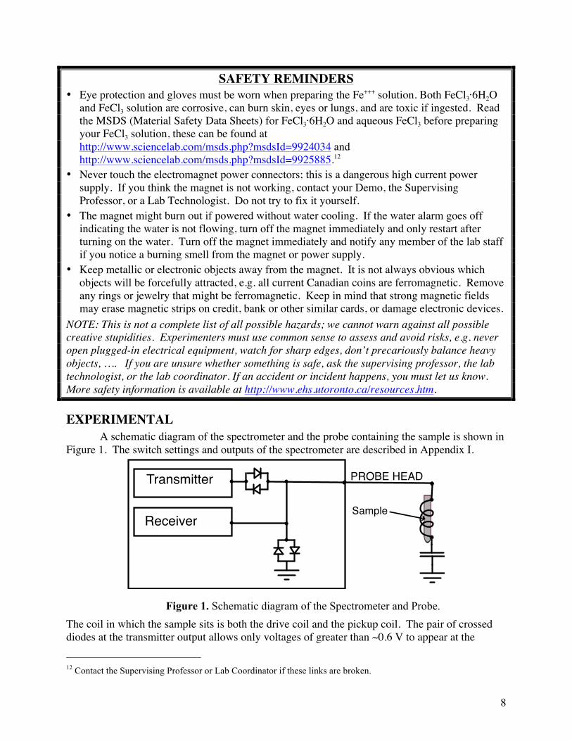
EXPERIMENTAL A schematic diagram of the spectrometer and the probe containing the sample is shown in
Figure 1. The switch settings and outputs of the spectrometer are described in Appendix I.
Figure 1. Schematic diagram of the Spectrometer and Probe. The coil in which the sample sits is both the drive coil and the pickup coil. The pair of crossed diodes at the transmitter output allows only voltages of greater than ~0.6 V to appear at the
12 Contact the Supervising Professor or Lab Coordinator if these links are broken.
Transmitter
Sample
PROBE HEAD
Receiver
9
sample. Thus when the transmitter is off, no low voltage noise from the transmitter is seen at the input of the receiver. The pair of crossed diodes to ground at receiver input protects the sensitive input of the receiver from the high voltages present when the transmitter is on.
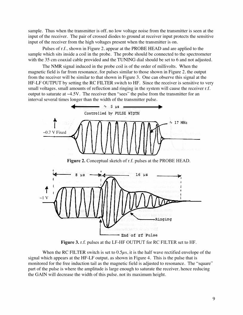
Pulses of r.f., shown in Figure 2, appear at the PROBE HEAD and are applied to the sample which sits inside a coil in the probe. The probe should be connected to the spectrometer with the 35 cm coaxial cable provided and the TUNING dial should be set to 6 and not adjusted.
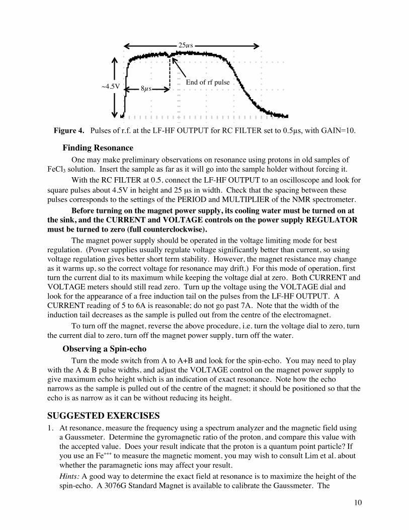
The NMR signal induced in the probe coil is of the order of millivolts. When the magnetic field is far from resonance, for pulses similar to those shown in Figure 2, the output from the receiver will be similar to that shown in Figure 3. One can observe this signal at the HF-LF OUTPUT by setting the RC FILTER switch to HF. Since the receiver is sensitive to very small voltages, small amounts of reflection and ringing in the system will cause the receiver r.f. output to saturate at ~4.5V. The receiver then “sees” the pulse from the transmitter for an interval several times longer than the width of the transmitter pulse.
Figure 2. Conceptual sketch of r.f. pulses at the PROBE HEAD.
Figure 3. r.f. pulses at the LF-HF OUTPUT for RC FILTER set to HF.
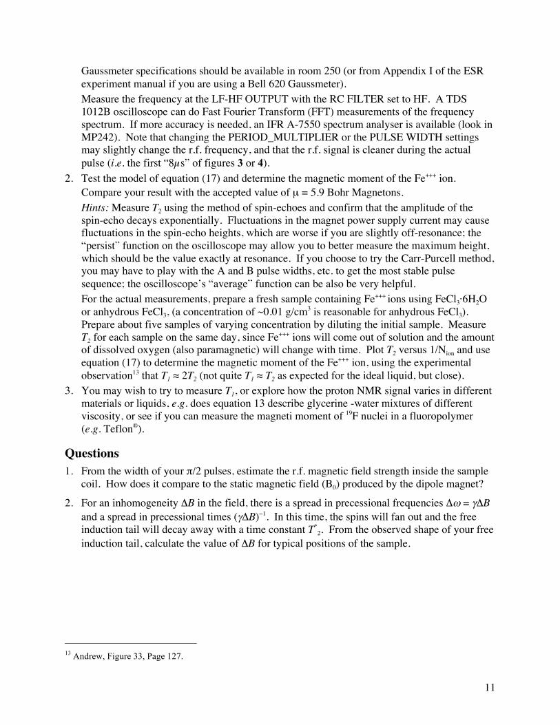
When the RC FILTER switch is set to 0.5µs, it is the half wave rectified envelope of the signal which appears at the HF-LF output, as shown in Figure 4. This is the pulse that is monitored for the free induction tail as the magnetic field is adjusted to resonance. The “square” part of the pulse is where the amplitude is large enough to saturate the receiver, hence reducing the GAIN will decrease the width of this pulse, not its maximum height.
~0.7 V Fixed
~1 V
10
Figure 4. Pulses of r.f. at the LF-HF OUTPUT for RC FILTER set to 0.5µs, with GAIN=10.
Finding Resonance One may make preliminary observations on resonance using protons in old samples of
FeCl3 solution. Insert the sample as far as it will go into the sample holder without forcing it. With the RC FILTER at 0.5, connect the LF-HF OUTPUT to an oscilloscope and look for
square pulses about 4.5V in height and 25 µs in width. Check that the spacing between these pulses corresponds to the settings of the PERIOD and MULTIPLIER of the NMR spectrometer.
Before turning on the magnet power supply, its cooling water must be turned on at the sink, and the CURRENT and VOLTAGE controls on the power supply REGULATOR must be turned to zero (full counterclockwise).
The magnet power supply should be operated in the voltage limiting mode for best regulation. (Power supplies usually regulate voltage significantly better than current, so using voltage regulation gives better short term stability. However, the magnet resistance may change as it warms up, so the correct voltage for resonance may drift.) For this mode of operation, first turn the current dial to its maximum while keeping the voltage dial at zero. Both CURRENT and VOLTAGE meters should still read zero. Turn up the voltage using the VOLTAGE dial and look for the appearance of a free induction tail on the pulses from the LF-HF OUTPUT. A CURRENT reading of 5 to 6A is reasonable; do not go past 7A. Note that the width of the induction tail decreases as the sample is pulled out from the centre of the electromagnet.
To turn off the magnet, reverse the above procedure, i.e. turn the voltage dial to zero, turn the current dial to zero, turn off the magnet power supply, turn off the water.
Observing a Spin-echo Turn the mode switch from A to A+B and look for the spin-echo. You may need to play
with the A & B pulse widths, and adjust the VOLTAGE control on the magnet power supply to give maximum echo height which is an indication of exact resonance. Note how the echo narrows as the sample is pulled out of the centre of the magnet; it should be positioned so that the echo is as narrow as it can be without reducing its height.
SUGGESTED EXERCISES 1. At resonance, measure the frequency using a spectrum analyzer and the magnetic field using
a Gaussmeter. Determine the gyromagnetic ratio of the proton, and compare this value with the accepted value. Does your result indicate that the proton is a quantum point particle? If you use an Fe+++ to measure the magnetic moment, you may wish to consult Lim et al. about whether the paramagnetic ions may affect your result. Hints: A good way to determine the exact field at resonance is to maximize the height of the spin-echo. A 3076G Standard Magnet is available to calibrate the Gaussmeter. The
25µs
8µs ~4.5V End of rf pulse
11
Gaussmeter specifications should be available in room 250 (or from Appendix I of the ESR experiment manual if you are using a Bell 620 Gaussmeter). Measure the frequency at the LF-HF OUTPUT with the RC FILTER set to HF. A TDS 1012B oscilloscope can do Fast Fourier Transform (FFT) measurements of the frequency spectrum. If more accuracy is needed, an IFR A-7550 spectrum analyser is available (look in MP242). Note that changing the PERIOD_MULTIPLIER or the PULSE WIDTH settings may slightly change the r.f. frequency, and that the r.f. signal is cleaner during the actual pulse (i.e. the first “8µs” of figures 3 or 4).
2. Test the model of equation (17) and determine the magnetic moment of the Fe+++ ion. Compare your result with the accepted value of µ = 5.9 Bohr Magnetons. Hints: Measure T2 using the method of spin-echoes and confirm that the amplitude of the spin-echo decays exponentially. Fluctuations in the magnet power supply current may cause fluctuations in the spin-echo heights, which are worse if you are slightly off-resonance; the “persist” function on the oscilloscope may allow you to better measure the maximum height, which should be the value exactly at resonance. If you choose to try the Carr-Purcell method, you may have to play with the A and B pulse widths, etc. to get the most stable pulse sequence; the oscilloscope’s “average” function can be also be very helpful. For the actual measurements, prepare a fresh sample containing Fe+++ ions using FeCl3·6H2O or anhydrous FeCl3, (a concentration of ~0.01 g/cm3 is reasonable for anhydrous FeCl3). Prepare about five samples of varying concentration by diluting the initial sample. Measure T2 for each sample on the same day, since Fe+++ ions will come out of solution and the amount of dissolved oxygen (also paramagnetic) will change with time. Plot T2 versus 1/Nion and use equation (17) to determine the magnetic moment of the Fe+++ ion, using the experimental observation13 that T1 ≈ 2T2 (not quite T1 ≈ T2 as expected for the ideal liquid, but close).
3. You may wish to try to measure T1, or explore how the proton NMR signal varies in different materials or liquids, e.g. does equation 13 describe glycerine -water mixtures of different viscosity, or see if you can measure the magneti moment of 19F nuclei in a fluoropolymer (e.g. Teflon®).
Questions 1. From the width of your π/2 pulses, estimate the r.f. magnetic field strength inside the sample
coil. How does it compare to the static magnetic field (B0) produced by the dipole magnet?
2. For an inhomogeneity ΔB in the field, there is a spread in precessional frequencies Δω = γΔB and a spread in precessional times (γΔB)−1. In this time, the spins will fan out and the free induction tail will decay away with a time constant T*
2. From the observed shape of your free induction tail, calculate the value of ΔB for typical positions of the sample.
13 Andrew, Figure 33, Page 127.
12
REFERENCES A. Abragam, “Principles of Nuclear Magnetism”, Clarendon Press, 1961. (QC 762 A23);. E.R. Andrew, “Nuclear Magnetic Resonance”, Cambridge University, 1958. (QC 753 A6 1958). N. Bloembergen, E.M. Purcell, and R.V. Pound, “Relaxation Effects in Nuclear Magnetic
Resonance Absorption”, Physical Review 73 (1948) 679-715. E. Fukushima and S.B.W. Roeder, “Experimental Pulse NMR: A Nuts and Bolts Approach”,
Addison-Wesley, 1981. (QC 762 F85). E.L. Hahn, “Free Nuclear Induction”, Physics Today, Vol. 11, No. 11, 1953. M. H. Levitt, Spin Dynamics: Basics of Nuclear Magnetic Resonance, 2nd Ed., John Wiley and
Sons (2008). A.R. Lim, C.S. Kim, S.H. Choh, Effect of Paramagnetic Ions in Aqueous Solution for Precision
Measurement of Proton Gyromagnetic Ratio, Bulletin of Magnetic Resonance 14 (1992) 240-245.
APPENDIX I: Spin-Lock Spectrometer Controls POWER: On/Off (…simple enough!) OUTPUT: Supplies pulses to the oscilloscope or spectrum analyzer. RC FILTER a) Shapes the output pulses. For the oscilloscope the setting should be 0.5, which produces
square 4.5V pulses , with a width of ~ 20µs depending slightly on other control settings. b) Use HF position when measuring the r.f. frequency. In the HF position, pulses coming from
OUTPUT are not the same size or shape as pulses applied to the sample but the r.f. frequency is the same. When measuring the r.f. frequency, the probe should be connected to the PROBE HEAD output since this affects the output frequency of the spectrometer.
GAIN: Amplification of the signal picked up in the probe. Usually turned to maximum. TUNING: Provides about a 1% change in the r.f. frequency. The spin-echo height is
maximum when TUNING is set to 6 and a 35 cm coaxial cable is used to connect the probe to the spectrometer. It is best to work with a fixed frequency and only adjust the magnetic field.
PROBE HEAD: Sends and receives r.f. pulses to and from the sample. Note that if one connects the PROBE HEAD output directly to an oscilloscope or spectrum analyzer, then this change in load will slightly alter the output frequency.
PERIOD-MULTIPLIER: Determines the rate at which the r.f. pulses are applied to the sample. When the PERIOD setting is at MAN., a pulse of r.f. is applied to the sample whenever the red MANUAL button is pressed.
MODE MODE A: Pulses of r.f. are applied to the sample with a period determined by PERIOD-
MULTIPLIER. PULSE B DELAY MULTIPLIER has no effect. MODE A+B: A first pulse (A) is followed by a second pulse (B). The period of the A pulse
is determined by PERIOD MULTIPLIER and the delay time between the A and B pulses is determined by PULSE B DELAY-MULTIPLIER.
MODE C.P.: Continuous pulses (e.g. for Carr-Purcell). After each A pulse there is a succession of B pulses. The spacing between the B pulses is determined by the position of the MODE switch and the C.P. SPACING MULTIPLIER. Note that the first B pulse follows the A pulse by a time equal to one half the C.P. SPACING. The function of the PULSE B DELAY-MULTIPLIER switch now changes to C.P. DURATION (see below the switch). C.P. DURATION determines how many B pulses there will be.
Example A PULSE PERIOD 4 × 10 ms C.P. SPACING 2 × 1 ms C.P. DURATION 2 × 10 ms There are 40 ms between A pulses, the B pulses occur every 2 ms, with the first B
pulse half the C.P. SPACING after the A pulse, and the B pulses repeat for 20 ms, i.e. there should be 10 B pulses following each A pulse.
A-PULSE WIDTH: Width of the A pulse or how long the r.f. is applied to the sample. B-PULSE WIDTH: Determines the width of the B pulse. B OUTPUT: Provides an output pulse every time there is a B pulse. May be used to trigger the