NMT EE 589 & UNM ME 482/582 ROBOT ENGINEERINGgeek.nmt.edu/~bruder/lectures/25_Oct_2012.pdf · 2012....

NMT EE 589 & UNM ME 482/582

ROBOT ENGINEERING

Dr. Stephen Bruder NMT EE 589 & UNM ME 482/582

© 2011, Dr. Stephen Bruder

6. Trajectory Generation 6.3.3 A Linear Segment With Parabolic Blends

Thursday 25th Oct 2012 ME 482/582: Robotics Engineering

It is often desirable to minimize the time to traverse a joint trajectory.

○ Would like to move at a max constant joint rate.

○ To minimize time employ max joint acceleration to get to this constant joint rate

Linear segment

Parabolic

Blend

Parabolic

Blend

Slide 2 / 12




Assume that we start from a position 𝜃(𝑡0) ≐ 𝜃0 and come to rest at a final point 𝜃(𝑡𝑓) ≐ 𝜃𝑓.

Furthermore, assume that the manipulator was initially at rest 𝜃 (𝑡0) = 0, and that it will come to rest at the final point 𝜃 (𝑡𝑓) = 0.

○ Let’s allow 𝑡0 = 0, for simplicity’s sake!! (can always compensate afterwards)

Segment 1 :

Assume a constant acceleration of 𝜃 𝑡 ≐ 𝑎. Using a Taylor series expansion:

Thus, the position at the end of this segment is (6.5)

0 0( ) ( )t t 2

00 0 0

2

0

0[ ]

[ ] ( ) ,2

, [0, )2

b

b

t tt t t t t t

ta t t

2

0 1( )2

bb

tt a

Slide 3 / 12




The velocity at any time during this segment is

Thus, the velocity at the end of this blend segment is (say) (6.6)

Segment 2 :

A constant velocity of 𝜃 (𝑡) ≐ 𝑣 (6.7)

and

( )t at

( )b bt a t v

1( ) ( )[ ] ,b b b f bt t t t t t t t

1 2( ) [ 2 ]f b f bt t t t v

( ) ( ) ,b b f bt t v t t t t

Slide 4 / 12




Segment 3 :

A constant acceleration of 𝜃 𝑡 ≐ −𝑎

Thus, the position at the end of this segment is (6.8)

and the velocity at the end of this blend segment is

2

2

[ [ ]]( ) ( )[ [ ]] ( ) , ( )

2

f b

f b f b f b f b f

t t tt t t t t t t t t t t t

2

2( )2

bf b f

tt vt a

( ) [ [ ]]

0

fff b t tt t

b

t v a t t t

v at

2

2

[ [ ]][ [ ]]

2

f b

f b

t t tv t t t a

Slide 5 / 12




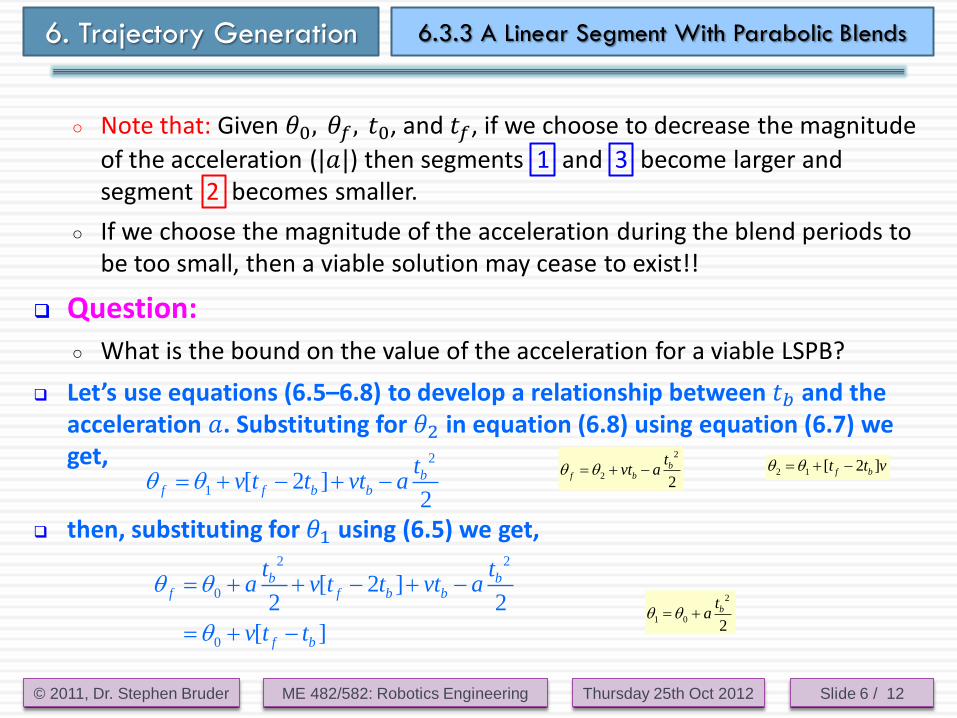
○ Note that: Given 𝜃0, 𝜃𝑓 , 𝑡0, and 𝑡𝑓, if we choose to decrease the magnitude

of the acceleration (|𝑎|) then segments 1 and 3 become larger and segment 2 becomes smaller.

○ If we choose the magnitude of the acceleration during the blend periods to be too small, then a viable solution may cease to exist!!

Question:

○ What is the bound on the value of the acceleration for a viable LSPB?

Let’s use equations (6.5–6.8) to develop a relationship between 𝑡𝑏 and the acceleration 𝑎. Substituting for 𝜃2 in equation (6.8) using equation (6.7) we get,

then, substituting for 𝜃1 using (6.5) we get,

2

1 [ 2 ]2

bf f b b

tv t t vt a

2 2

0

0

[ 2 ]2 2

[ ]

b bf f b b

f b

t ta v t t vt a

v t t

2

22

bf b

tvt a 2 1 [ 2 ]f bt t v

2

1 02

bta

Slide 6 / 12




Recalling the expression for 𝑣 from equation (6.6) gives

Solving for this quadratic in 𝑡𝑏 gives

○ Intuitively, from the diagram if 𝑡𝑏 ≥𝑡𝑓

2 , then a viable solution ceases to

exist!! or

(6.9)

0 [ ]f b f bat t t

2

0[ ] 0b f b fat at t

2 2

04 [ ]

2

f f f

b

at a t at

a

0

2

4[ ]f

f

at

2 2

04 [ ]

2 2

f ffa t at

a

bv a t

2 2

04 [ ] 0f fa t a

Slide 7 / 12




○ At the point where the equality holds (𝑎 =4[𝜃𝑓−𝜃0

𝑡𝑓2 ), the linear segment is

of length zero. This is known as a bang-bang parabolic blend!!

Slide 8 / 12




0 1 2 3 4 5 6 7 8 9 100

50

100

LSPB: 0=10°,

f=84°, t

f=10 sec, a=10 °/s2, v=8 °/s, t

b=0.8 sec

in

0 1 2 3 4 5 6 7 8 9 100

5

10

d/d

t in

/s

0 1 2 3 4 5 6 7 8 9 10

-10

0

10

d2/d

t2 in

/s2

Time in sec

0 1 2 3 4 5 6 7 8 9 100

50

100

LSPB: 0=10°,

f=84°, t

f=10 sec, a=5 °/s2, v=9 °/s, t

b=1.8 sec

in

0 1 2 3 4 5 6 7 8 9 100

5

10

d/d

t in

/s

0 1 2 3 4 5 6 7 8 9 10

-5

0

5

d2/d

t2 in

/s2

Time in sec

0 1 2 3 4 5 6 7 8 9 100

50

100

LSPB: 0=10°,

f=84°, t

f=10 sec, a=3 °/s2, v=15 °/s, t

b=5.0 sec

in

0 1 2 3 4 5 6 7 8 9 100

10

20

d/d

t in

/s

0 1 2 3 4 5 6 7 8 9 10

-20

2

d2/d

t2 in

/s2

Time in sec

0 2

2

4[ ]2.96 /

f

f

a st

A Bang-Bang

Parabolic Blend

a=10 /s2 a=5 /s2

a = 3 /s2

Slide 9 / 12

matlab_files/section6


6. Trajectory Generation 6.4 Cartesian Space Schemes


Now specify the path in term of the tool pose

Can describe straight line Cartesian trajectories

Both position and orientation

Requires an inverse kinematic computation at each point

Describing the orientation can be challenging

○ Euler angles?

○ RPY angles?

○ Rotation matrix?

○ Angle/axis representation?

Slide 10 / 12


6. Trajectory Generation 6.4 An Example: Joint vs Cartesian


A Puma 560 example

○ Compare a Joint space vs Cartesian space trajectory

Slide 11 / 12

MATLAB Example

“Traj_gen1.m”

matlab_files/section6


6. Trajectory Generation 6.4 An Example: Joint vs Cartesian


0 0.2 0.4 0.6 0.8 1 1.2 1.4 1.6 1.8 2-150

-100

-50

0

50

100

150

200Joint Space TG: Joint Angle Time History

Time in sec

Join

t A

ngle

in

1

2

3

4

5

6

0 0.2 0.4 0.6 0.8 1 1.2 1.4 1.6 1.8 2-150

-100

-50

0

50

100

150

200Cartesian Space TG: Joint Angle Time History

Time in sec

Cart

esia

n A

ngle

in

1

2

3

4

5

6

0 0.2 0.4 0.6 0.8 1 1.2 1.4 1.6 1.8 2

-0.5

0

0.5

Joint Space TG: Positional Time History

Tool P

ositio

n in m

px

py

pz

0 0.2 0.4 0.6 0.8 1 1.2 1.4 1.6 1.8 2

-1

-0.5

0

0.5

1

Joint Space TG: Axis of Rotation

Norm

aliz

ed U

nits

kx

ky

kz

0 0.2 0.4 0.6 0.8 1 1.2 1.4 1.6 1.8 2

100

150

200Joint Space TG: Angle of Rotation

Time in sec

Angle

in

Join

t Spa

ce T

raje

ctory

Gene

ration

Ca

rtesia

n Sp

ace

Tra

ject

ory

Gene

ration

Slide 12 / 12

0 0.2 0.4 0.6 0.8 1 1.2 1.4 1.6 1.8 2

-0.5

0

0.5

Cartesian Space TG: Positional Time History

Tool P

ositio

n in m

px

py

pz

0 0.2 0.4 0.6 0.8 1 1.2 1.4 1.6 1.8 2

-1

-0.5

0

0.5

1

Cartesian Space TG: Axis of Rotation

Norm

aliz

ed U

nits

kx

ky

kz

0 0.2 0.4 0.6 0.8 1 1.2 1.4 1.6 1.8 2

100

150

200Cartesian Space TG: Angle of Rotation

Time in sec

Angle

in

Date post:	04-Apr-2021
Category:	Documents
Upload:	others
View:	0 times
Download:	0 times

NMT EE 589 & UNM ME 482/582 ROBOT ENGINEERINGgeek.nmt.edu/~bruder/lectures/25_Oct_2012.pdf · 2012....

Documents