IX - 1

ààà`zzzÚÚÚüüüNNNCCC©©©ØØتªªÂÂÂ

1Êù:Äu5C©Øª PC¦)EÜà`z¯KÂ

Contraction methods for composite convexoptimization based on the PC Algorithms for LVIs

HEÆêÆX Û])hebma@nju.edu.cn

IX - 2

ÁÁÁ. þ­VÊc,·uL¦)üN5C©Øª(9à

g`z)ÝKÂ . ù¦<^5¦)A^¯Kké

ÐLy. 3?naÅì<¯Kþ,åÙ¦ØUO

^[3, 11, 12].©0XÛòùí2,^5¦)EÜà`z¯K.

1 Introduction

In the 1990s, we have published some projection and contraction algorithms for

solving monotone linear variational inequalities [5, 6]. These algorithms can be

applied to solve the constrained convex optimization problems

min1

2xTHx+ cTx |x ∈ X (1.1)

and

min1

2xTHx+ cTx |Ax = b(or≥ b), x ∈ X, (1.2)

where H ∈ <n×n is a symmetric positive semi-definite matrix, A ∈ <m×n,

b ∈ <m, c ∈ <n and X ⊂ <n is a closed convex set. The purpose of this

IX - 3

article is to develop such algorithms to solve the following composite convex

optimization problems:

minθ(x) +1

2xTHx+ cTx |x ∈ X (1.3)

and

minθ(x) +1

2xTHx+ cTx |Ax = b(or≥ b), x ∈ X, (1.4)

where θ(x) : <n → < is a convex function (not necessarily smooth),

H, A, b, c and X are the same as described in (1.1) and (1.2).

Throughout this article, we assume that the solution set (1.3) and (1.4) are

nonempty. In addition, we assume that for any given constant r > 0 and vector

a ∈ <n, the subproblem

minθ(x) +r

2‖x− a‖2 | x ∈ X (1.5)

has a closed-form solution or can be efficiently computed with a high precision.

The analysis of this note is based on the following lemma (proof is omitted here).

IX - 4

Lemma 1.1 Let X ⊂ <n be a closed convex set, θ(x) and f(x) be convex

functions and f(x) is differentiable on an open set which includes Ω. Assume

that the solution set of the minimization problem minθ(x) + f(x) |x ∈ Xis nonempty. Then,

x∗ ∈ arg minθ(x) + f(x) |x ∈ X (1.6a)

if and only if

x∗ ∈ X , θ(x)− θ(x∗) + (x− x∗)T∇f(x∗) ≥ 0, ∀x ∈ X . (1.6b)

2 The algorithms for solving (1.3) based on P-CAlgorithm for the problem (1.1)

In (1.3), since the θ(x) is convex and H is semidefinite, by using Lemma 1.1, the

optimal solution of (1.3), say x∗, satisfies

x∗ ∈ X , θ(x)− θ(x∗) + (x− x∗)T (Hx∗ + c) ≥ 0, ∀x ∈ X . (2.1)

IX - 5

2.1 Key inequality for solving min1

2xTHx+ cTx |x ∈ X

Set θ(x) = 0 in (1.3), it is reduced to the problem (1.1) whose optimal solution

x∗ satisfies

x∗ ∈ X , (x− x∗)T (Hx∗ + c) ≥ 0, ∀x ∈ X . (2.2)

For solving (1.1) (or its equivalent (2.2)), we have proposed a class of projection

and contraction algorithms [5, 6]. These algorithms are based on constructing the

descent direction of the distance function 12‖x− x

∗‖2G, where G is some

symmetric positive definite matrix.

For given xk ∈ <n and β > 0, let

xk = PX [xk − β(Hxk + c)]. (2.3)

xk is the optimal solution of (1.1) (or its equivalent (2.2)) if and only if xk = xk.

IX - 6

The projector xk is the solution of the minimization problem,

xk = arg min1

2‖x− [xk − β(Hxk + c)]‖2 |x ∈ X.

According to Lemma 1.1, we have

xk ∈ X , (x− xk)T xk − [xk − β(Hxk + c)] ≥ 0, ∀x ∈ X .

Set the any vector x ∈ X in the above inequality by a solution point x∗, it follows

that

(xk − x∗)T (xk − xk)− β(Hxk + c) ≥ 0. (2.4)

On the other hand, since xk ∈ X , it follows from (2.2) that

(xk − x∗)Tβ(Hx∗ + c) ≥ 0. (2.5)

Adding (2.4) and (2.5), we get

(xk − x∗)T (xk − xk)− βH(xk − x∗) ≥ 0.

IX - 7

The above inequality can be rewritten as

(xk − x∗)− (xk − xk)T (xk − xk)− βH(xk − x∗) ≥ 0.

Finally, by using the semi-positiveness of H , we get

(xk − x∗)T (I + βH)(xk − xk) ≥ ‖xk − xk‖2. (2.6)

The above inequality is the main basis for building the projection contraction

algorithms for solving (1.1) (and its equivalent variational inequality (2.2)). We

hope to establish the same inequality for the problem (1.3).

2.2 Key inequality for solving minθ(x)+ 12xTHx+cTx|x∈X

Our task is to solve (1.3). The purpose of this subsection is to construct the same

key-inequality as (2.6). For given xk and β > 0, we let

xk = arg minθ(x) +1

2β‖x− [xk − β(Hxk + c)]‖2 |x ∈ X. (2.7)

IX - 8

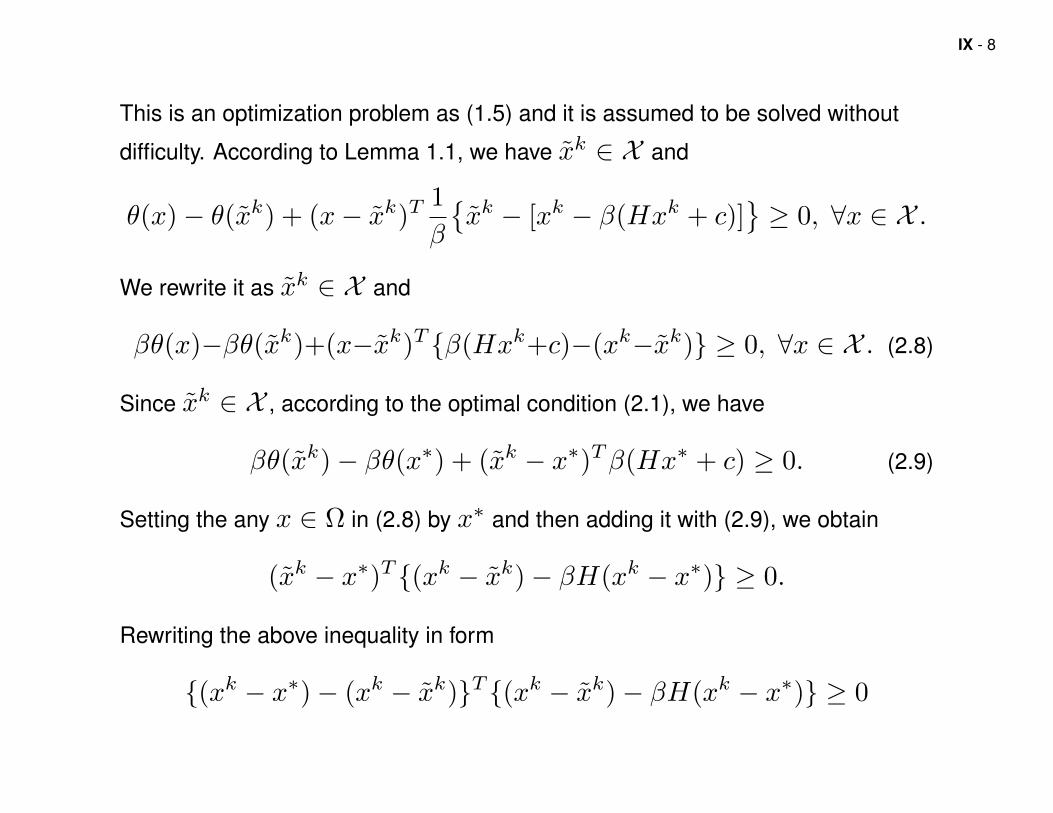
This is an optimization problem as (1.5) and it is assumed to be solved without

difficulty. According to Lemma 1.1, we have xk ∈ X and

θ(x)− θ(xk) + (x− xk)T1

β

xk − [xk − β(Hxk + c)]

≥ 0, ∀x ∈ X .

We rewrite it as xk ∈ X and

βθ(x)−βθ(xk)+(x−xk)T β(Hxk+c)−(xk−xk) ≥ 0, ∀x ∈ X . (2.8)

Since xk ∈ X , according to the optimal condition (2.1), we have

βθ(xk)− βθ(x∗) + (xk − x∗)Tβ(Hx∗ + c) ≥ 0. (2.9)

Setting the any x ∈ Ω in (2.8) by x∗ and then adding it with (2.9), we obtain

(xk − x∗)T (xk − xk)− βH(xk − x∗) ≥ 0.

Rewriting the above inequality in form

(xk − x∗)− (xk − xk)T (xk − xk)− βH(xk − x∗) ≥ 0

IX - 9

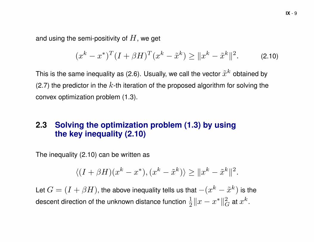
and using the semi-positivity of H , we get

(xk − x∗)T (I + βH)T (xk − xk) ≥ ‖xk − xk‖2. (2.10)

This is the same inequality as (2.6). Usually, we call the vector xk obtained by

(2.7) the predictor in the k-th iteration of the proposed algorithm for solving the

convex optimization problem (1.3).

2.3 Solving the optimization problem (1.3) by usingthe key inequality (2.10)

The inequality (2.10) can be written as

〈(I + βH)(xk − x∗), (xk − xk)〉 ≥ ‖xk − xk‖2.

Let G = (I + βH), the above inequality tells us that−(xk − xk) is the

descent direction of the unknown distance function 12‖x− x

∗‖2G at xk.

IX - 10

We take

xk+1(α) = xk − α(xk − xk) (2.11)

as the step length α dependent new iterate. In order to shorten the distance

‖x− x∗‖2(I+βH), we consider the following α-dependent benefit

ϑk(α) = ‖xk − x∗‖2(I+βH) − ‖xk+1(α)− x∗‖2(I+βH). (2.12)

By using (2.10), we obtain

ϑk(α) = ‖xk − x∗‖2(I+βH) − ‖xk − x∗ − α(xk − xk)‖2(I+βH)

= 2α(xk − x∗)T (I + βH)(xk − xk)

−α2‖xk − xk‖2(I+βH). (2.13)

By using the (2.10), we have the following theorem.

Theorem 2.1 For given xk and any β > 0, let xk be a predictor generated by

(2.7) and xk+1(α) be updated by (2.11). Then for any α > 0, we have

ϑk(α) ≥ qk(α), (2.14)

IX - 11

where ϑk(α) is defined by (2.12) and

qk(α) = 2α‖xk − xk‖2 − α2‖xk − xk‖2(I+βH). (2.15)

Proof. The assertion of this theorem follows directly from (2.13) and (2.10). 2

Now, qk(α) is a lower bound function of ϑk(α). The quadratic function qk(α)

reaches its maximum at

α∗k =‖xk − xk‖2

(xk − xk)T (I + βH)(xk − xk). (2.16)

We use

xk+1 = xk − γα∗k(xk − xk), γ ∈ (0, 2) (2.17)

to determine the new iterate xk+1. By using (2.15) and (2.16), we get

q(γα∗k) = 2γα∗k‖xk − xk‖2 − γ2α∗k(α∗k‖xk − xk‖2(I+βH)

)= γ(2− γ)α∗k‖xk − xk‖2. (2.18)

IX - 12

Thus, the profit of the k-th iteration

ϑ(γα∗k) = ‖xk − x∗‖2(I+βH) − ‖xk+1 − x∗‖2(I+βH)

≥ q(γα∗k) = γ(2− γ)α∗k‖xk − xk‖2. (2.19)

Theoretically ϑ(γα∗k) > 0 when γ ∈ (0, 2), usually, we take γ ∈ [1.2, 1.8].

O α* γα*

q(α)

ϑ(α)

α

Fig. 1 It is suggested to take γ ∈ [1.2, 1.8]

IX - 13

For solving the composite convex optimization problem (1.3), we use (2.7) to

generate the predictor xk and (2.17) to update the corrector xk+1. Together with

some strategy for adjusting the parameter β, we have the following algorithm.

Algorithm 2.1 Prediction-Correction method for solving the composite convex opti-

mization problem (1.3):

Start with given x0 and β > 0. For k = 0, 1, . . ., do:

1. Prediction: xk = arg minθ(x)+ 12β ‖x−[xk−β(Hxk+c)]‖2 |x ∈ X.

2. Correction: xk+1 = xk − γα∗k(xk − xk),

where α∗k =‖xk − xk‖2

(xk − xk)T (I + βH)(xk − xk)and γ ∈ (0, 2).

3. Adjust the parameter β if necessary

r =β‖xk − xk‖2H‖xk − xk‖2

, β =

(β/r) ∗ 0.9, if r > 1 or r < 0.4;

β, otherwise.

k := k + 1 and go to 1.

IX - 14

According to our numerical experiments, the parameter β should be selected in

range25‖x

k − xk‖ ≤ β‖xk − xk‖2H ≤ ‖xk − xk‖.

We can also adjust the parameters every five or ten iterations. In practical, after

some iterations, the algorithm will automatically find a suitable fixed β.

Theorem 2.2 For solving the composite convex optimization problem (1.3), the

sequence xk generated by Algorithm 2.1 with fixed β > 0 satisfies

‖xk+1−x∗‖2(I+βH) ≤ ‖xk−x∗‖2(I+βH)−

γ(2− γ)

‖I + βH‖‖xk−xk‖2. (2.20)

Proof. From (2.16) we have α∗k ≥ 1‖I+βH‖ . Together with (2.19), it follows the

assertion (2.20) directly. 2

Generally speaking, whether the selection of parameters is appropriate or not, it

will affect the convergence speed. Without loss of the generality, Theorem 2.2

gives us the key inequality for the convergence of Algorithm 2.1.

IX - 15

3 The algorithms for solving (1.4) based on P-CAlgorithm for the problem (1.2)

The Lagrangian function of the linearly constrained optimization problem (1.4) is

L(x, λ) = θ(x) +1

2xTHx+ cTx− λT (Ax− b),

which is defined on X × Λ and where

Λ =

<m, if the lineary constraints in (1.4) is Ax = b,

<m+ , if the lineary constraints in (1.4) is Ax ≥ b.

Let (x∗, λ∗) ∈ X × Λ be a saddle point of the Lagrangian function, we have

Lλ∈<m(x∗, λ) ≤ L(x∗, λ∗) ≤ Lx∈X (x, λ∗).

This tells us that (x∗, λ∗) ∈ X × Λ andL(x, λ∗)− L(x∗, λ∗) ≥ 0, ∀x ∈ X ,L(x∗, λ∗)− L(x∗, λ) ≥ 0, ∀λ ∈ Λ.

IX - 16

Thus, finding a saddle point of the Lagrange function is equivalent to finding

(x∗, λ∗) ∈ X × Λ such thatθ(x)− θ(x∗) + (x− x∗)T(Hx∗+ c−ATλ∗) ≥ 0, ∀x ∈ X ,

(λ− λ∗)T (Ax∗ − b) ≥ 0, ∀λ ∈ Λ.(3.1)

The above variational inequality can be written in a compact form

u∗ ∈ Ω, θ(x)− θ(x∗) + (u− u∗)T (Mu∗ + q) ≥ 0, ∀u ∈ Ω, (3.2a)

where

u =

(x

λ

), M =

(H −AT

A 0

), q =

(c

−b

)and Ω = X×Λ.

(3.2b)

Although the matrix M is not symmetric, however, for any u, we have uTMu =

xTHx ≥ 0. The variational inequality (3.2) is monotone.

IX - 17

3.1 Key inequality for solving the minimization problem

min12xTHx+ cTx |Ax = (or ≥) b, x ∈ X

Set θ(x) = 0 (1.4), the problem is reduced to the linear constrained quadratic

programming (1.2), the related variational inequality (3.2) is reduced to

u∗ ∈ Ω, (u− u∗)T (Mu∗ + q) ≥ 0, ∀u ∈ Ω, (3.3a)

where

u =

x

λ

, M =

H −AT

A 0

, q =

c

−b

and Ω = X × Λ.

(3.3b)

For solving (1.2) (or its equivalent (3.3)), we have proposed a projection and

contraction method [5] whose search direction is established in the following way.

First, for given uk ∈ <m+n and β > 0, let

uk = PΩ[uk − β(Muk + q)]. (3.4)

IX - 18

Since

uk = arg min1

2‖u− [uk − β(Muk + q)]‖2|u ∈ Ω,

according to Lemma 1.1, it follows that

uk ∈ Ω, (u− uk)T uk − [uk − β(Muk + q)] ≥ 0, ∀u ∈ Ω.

Setting the any u ∈ Ω in the above inequality by u∗, we get

(uk − u∗)T (uk − uk)− β(Muk + q) ≥ 0. (3.5)

Because uk ∈ Ω and β > 0, according to (3.3a), we have

(uk − u∗)Tβ(Mu∗ + q) ≥ 0. (3.6)

Adding the above two inequalities, we get

(uk − u∗)T (uk − uk)− βM(uk − u∗) ≥ 0. (3.7)

It can be written as

(uk − u∗)− (uk − uk)T (uk − uk)− βM(uk − u∗) ≥ 0.

IX - 19

Consequently, using the semi-positivity of M (vTMv ≥ 0), it follows that

(uk − u∗)T (I + βMT )(uk − uk) ≥ ‖uk − uk‖2, ∀u∗ ∈ Ω∗. (3.8)

The above inequality is the main basis for building the projection and contraction

algorithms for solving the linearly constrained convex quadratic optimization (1.2)

(and its equivalent variational inequality (3.2)). We hope to establish the same

inequality for the composite optimization problem (1.4).

3.2 Key inequality for solving the minimization problemminθ(x) + 1

2xTHx+ cTx |Ax = (or ≥) b, x ∈ X

Our task is to solve the problem (1.4). This subsection will construct the same

key-inequality as (3.8). For given uk = (xk, λk) and β > 0, let

xk = arg minθ(x) +1

2β‖x− [xk − β(Hxk + c−ATλk)]‖2 |x ∈ X

(3.9a)

IX - 20

and

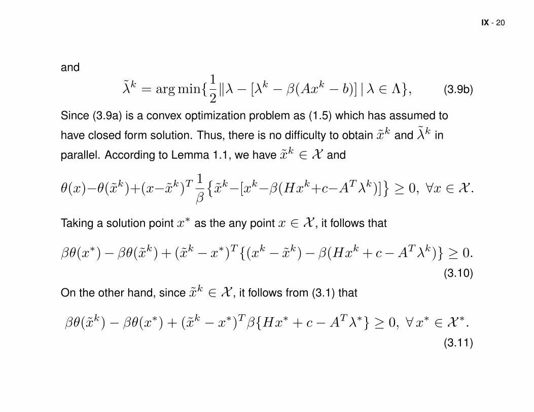
λk = arg min1

2‖λ− [λk − β(Axk − b)] |λ ∈ Λ, (3.9b)

Since (3.9a) is a convex optimization problem as (1.5) which has assumed to

have closed form solution. Thus, there is no difficulty to obtain xk and λk in

parallel. According to Lemma 1.1, we have xk ∈ X and

θ(x)−θ(xk)+(x−xk)T1

β

xk−[xk−β(Hxk+c−ATλk)]

≥ 0, ∀x ∈ X .

Taking a solution point x∗ as the any point x ∈ X , it follows that

βθ(x∗)− βθ(xk) + (xk − x∗)T (xk − xk)− β(Hxk + c−ATλk) ≥ 0.

(3.10)

On the other hand, since xk ∈ X , it follows from (3.1) that

βθ(xk)− βθ(x∗) + (xk − x∗)TβHx∗ + c−ATλ∗ ≥ 0, ∀x∗ ∈ X ∗.(3.11)

IX - 21

Adding (3.10) and (3.11), we obtain

(xk − x∗)T (xk − xk)− β[H(xk − x∗)−AT (λk − λ∗)] ≥ 0. (3.12)

For (3.9b), according to Lemma 1.1, we have

λk ∈ Λ, (λ− λk)Tλk − [λk − β(Axk − b)]

≥ 0, ∀ λ ∈ Λ.

Set the fixed any point λ ∈ Λ in the last inequality by λ∗, it follows that

(λk − λ∗)T (λk − λk)− β(Axk − b) ≥ 0. (3.13)

On the other hand, since λk ∈ Λ, according the second part of (3.1), we have

(λk − λ∗)Tβ(Ax∗ − b) ≥ 0. (3.14)

Adding (3.13) and (3.14), it follows that

(λk − λ∗)T (λk − λk)− βA(xk − x∗) ≥ 0. (3.15)

IX - 22

Write (3.12) and (3.15) together, xk − x∗

λk − λ∗

T xk − xk

λk − λk

− βH −AT

A 0

xk − x∗

λk − λ∗

≥ 0.

Using the notation in (3.3), it can be written as

(uk − u∗)T (uk − uk)− βM(uk − u∗) ≥ 0.

Clearly, it is same inequality as (3.7) in §3.1. It can be written as

(uk − u∗)− (uk − uk)T (uk − uk)− βM(uk − u∗) ≥ 0.

Consequently, using the semi-positivity of M (vTMv ≥ 0), it follows that

(uk − u∗)T (I + βMT )(uk − uk) ≥ ‖uk − uk‖2, ∀u∗ ∈ Ω∗. (3.16)

This is the same key inequality as (3.8). For solving the linearly constrained

composite convex optimization problem (1.4), we call the vector uk = (xk, λk)

obtained from (3.9) a predictor in the k-iteration.

IX - 23

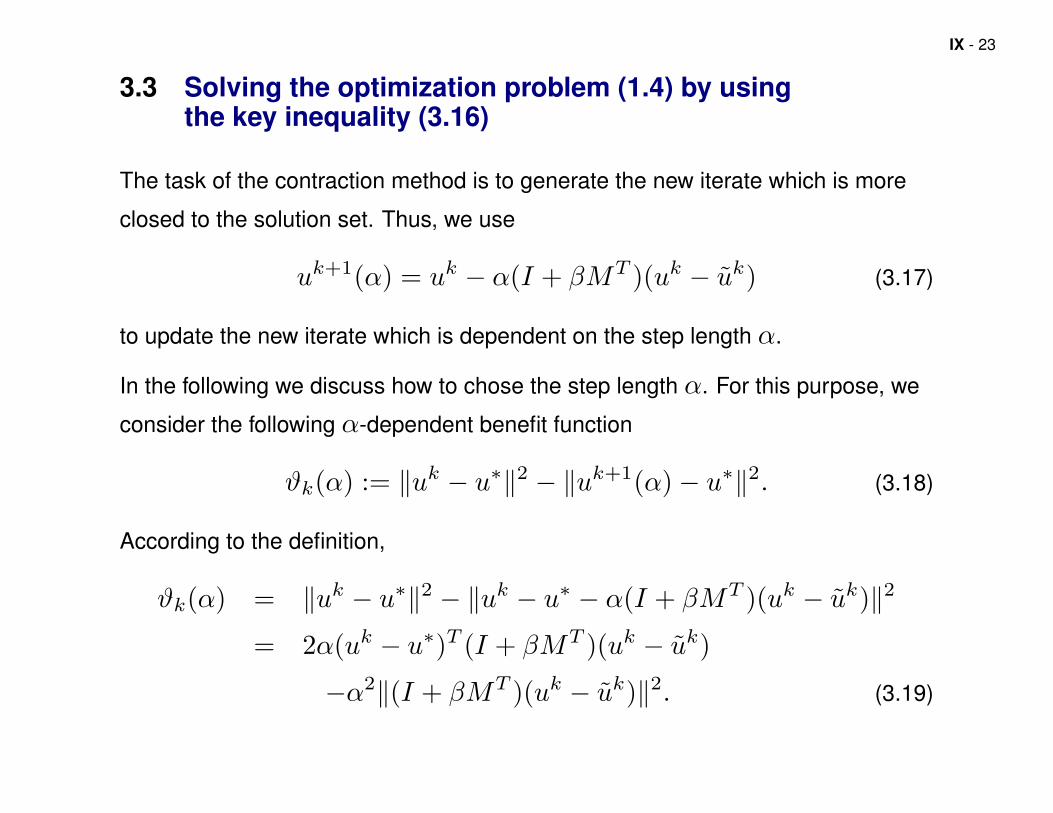
3.3 Solving the optimization problem (1.4) by usingthe key inequality (3.16)

The task of the contraction method is to generate the new iterate which is more

closed to the solution set. Thus, we use

uk+1(α) = uk − α(I + βMT )(uk − uk) (3.17)

to update the new iterate which is dependent on the step length α.

In the following we discuss how to chose the step length α. For this purpose, we

consider the following α-dependent benefit function

ϑk(α) := ‖uk − u∗‖2 − ‖uk+1(α)− u∗‖2. (3.18)

According to the definition,

ϑk(α) = ‖uk − u∗‖2 − ‖uk − u∗ − α(I + βMT )(uk − uk)‖2

= 2α(uk − u∗)T (I + βMT )(uk − uk)

−α2‖(I + βMT )(uk − uk)‖2. (3.19)

IX - 24

Theorem 3.1 For given uk and any β > 0, let uk be a predictor generated by

(3.9) and uk+1(α) be updated by (3.17). Then for any α > 0, we have

ϑk(α) ≥ qk(α), (3.20)

where ϑk(α) is defined by (3.18) and

qk(α) = 2α‖uk − uk‖2 − α2‖(I + βMT )(uk − uk)‖2. (3.21)

Proof. The assertion of this theorem follows from (3.19) and (3.16) directly. 2

Theorem 3.1 tells us qk(α) is a lower bound function of the profit function ϑk(α).

The quadratic function qk(α) (3.21) reaches its maximum at

α∗k = argmaxqk(α) =‖uk − uk‖2

‖(I + βMT )(uk − uk)‖2. (3.22)

Notice that our intention is to maximize the quadratic profit function ϑk(α) (see

(3.19)), which includes the unknown solution u∗. As a remedy, we maximize its

lower bound function qk(α).

IX - 25

In the practical computation, we take a γ ∈ [1, 2) and

uk+1 = uk − γα∗k(I + βMT )(uk − uk), (3.23)

to produce the new iterate. The reason to take γ ∈ [1, 2) is illustrated in Fig. 1 of

§2.3. Using (3.18) and (3.20), the new iterate uk+1 updated by (3.23) satisfies

‖uk+1 − u∗‖2 ≤ ‖uk − u∗‖2 − qk(γα∗k). (3.24)

According to the definitions of qk(α) and α∗k (see (3.21) and (3.22)), we get

qk(γα∗k) = 2γα∗k‖uk − uk‖2 − γ2α∗k(α∗k‖(I + βMT )(uk − uk)‖2)

= 2γα∗k‖uk − uk‖2 − γ2α∗k‖uk − uk‖2

= γ(2− γ)α∗k‖uk − uk‖2.

Thus, from (3.24) we get

‖uk+1 − u∗‖2 ≤ ‖uk − u∗‖2 − γ(2− γ)α∗k‖uk − uk‖2. (3.25)

IX - 26

Algorithm 3.1 Prediction-Correction method for solving the composite convex opti-

mization problem (1.4):

Start with given u0 = (x0, λ0) and β > 0. For k = 0, 1, . . ., do:

1. Prediction:

xk = arg minθ(x) + 12β ‖x− [xk − β(Hxk + c−ATλk)]‖2 |x ∈ X

and λk = arg min 12‖λ− [λk − β(Axk − b)] |λ ∈ Λ.

2. Correction: uk+1 = uk − γα∗k(I + βMT )(uk − uk),

where α∗k =‖uk − uk‖2

‖(I + βMT )(uk − uk)‖2. and γ ∈ (0, 2).

3. Adjust the parameter β if necessary

r =‖(I + βMT )(uk − uk)‖

‖uk − uk‖, β =

β ∗ (2.5/r) if r > 3

β ∗ (2.5/r) if r < 2

β otherwise.

k := k + 1 and go to 1.

IX - 27

For solving the problem (1.4), the k-th iteration of the Algorithm3.1 start from uk,

produces the predictor uk by (3.9), and updated the new iterate uk+1 by (3.23).

For this algorithm, we have the following theorem.

Theorem 3.2 Let uk be the sequence generated by the Algorithm3.1 for the

problem (1.4). Then we have

‖uk+1 − u∗‖2 ≤ ‖uk − u∗‖2 − γ(2− γ)

‖I + βMT ‖2‖uk − uk‖2. (3.26)

Proof. In fact, by using (3.22), we get

α∗k ≥1

‖I + βMT ‖2.

Thus, it follows from (3.25) that

qk(γα∗k) ≥ γ(2− γ)

‖I + βMT ‖2‖uk − uk‖2.

Substituting it in (3.24), the assertion (3.26) follows directly. 2

IX - 28

Remark Since the predictor uk generated by (3.9) satisfies (3.16), as in [6], we

can take

uk+1 = uk − γ(I + βM)−1(uk − uk) (3.27)

as the new iterate. For G = (I + βMT )(I + βM), by using (3.16), we get

‖uk+1 − u∗‖2G = ‖(uk − u∗)− γ(I + βM)−1(uk − uk)‖2G= ‖uk − u∗‖2G − 2γ(uk − u∗)T (I + βM)T (uk − uk)

+ γ2‖(I + βM)−1(uk − uk)‖2G≤ ‖uk − u∗‖2G − γ(2− γ)‖uk − uk‖2.

Thus, for solving the optimization problem (1.4), if we use (3.9) to offer the

predictor and (3.27) to update the new iterate, then the sequence uk satisfies

‖uk+1 − u∗‖2G ≤ ‖uk − u∗‖2G − γ(2− γ)‖uk − uk‖2.

IX - 29

4 Convergence rate of the Algorithm 2.1

This section studies the convergence rate of the Algorithm 2.1 for the composite

convex optimization problem (1.3) (or its equivalent variational inequality (2.1)) :

θ(x)− θ(x∗) + (x− x∗)T (Hx∗ + c) ≥ 0, ∀x ∈ X . (4.1)

For given xk ∈ <n, the predictor xk in Algorithm 2.1 is offered by (2.7). The new

iterate of the k-th iteration of Algorithm 2.1 is updated by

xk+1 = xk − γα∗k(xk − xk), (4.2)

where

α∗k =‖xk − xk‖2

‖xk − xk‖2G, G = I + βH and γ ∈ (0, 2). (4.3)

It was proved [6] that the sequence xk generated by the Algorithm 2.1 satisfies

‖xk+1 − x∗‖2G ≤ ‖xk − x∗‖2G − γ(2− γ)α∗k‖xk − xk‖2. (4.4)

IX - 30

Recall that X ∗ can be characterized as (see Theorem 2.1 in [8])

X ∗ =⋂x∈X

x ∈ X : θ(x)− θ(x) + (x− x)T (Hx+ c) ≥ 0

.

This implies that x ∈ X is an approximate solution of (4.1) with the accuracy ε if

it satisfies

x ∈ X and infx∈D(x)

θ(x)− θ(x) + (x− x)T (Hx+ c)

≥ −ε,

where

D(x) = x ∈ X | ‖x− x‖ ≤ 1.

In this section, we show that, for given ε > 0, in O(1/ε) iterations the Algorithm

2.1 can find a x such that

x ∈ Ω and supx∈D(x)

(θ(x)− θ(x)

)+ (x− x)T (Hx+ c)

≤ ε, (4.5)

where

D(x) = x ∈ Ω | ‖x− x‖ ≤ 1.

IX - 31

In this sense, we will establish the algorithmic convergence complexity for the

Algorithm 2.1.

4.1 Main theorem for complexity analysis

This subsection proves some main theorems for the complexity analysis. Now, we

prove the key inequality for the complexity analysis of the Algorithm 2.1.

Theorem 4.1 For given xk ∈ <n, let xk be generated by (2.7). If he new iterate

xk+1 is updated by (4.2) with any γ ∈ (0, 2), then we have

γα∗kβθ(x)− θ(xk) + (x− xk)T (Hx+ c)

≥ 1

2

(‖x− xk+1‖2G − ‖x− xk‖2G

)+

1

2qk(γ), ∀x ∈ Ω, (4.6)

where

qk(γ) = γ(2− γ)α∗k‖xk − xk‖2. (4.7)

Proof. Since xk is the solution of (2.7), we have (see (2.8))

βθ(x)− βθ(xk) + (x− xk)T β(Hxk + c)− (xk − xk) ≥ 0, ∀x ∈ X .

IX - 32

Thus, we have

βθ(x)−βθ(xk)+(x− xk)Tβ(Hxk+c) ≥ (x− xk)T (xk− xk), ∀x ∈ X .

Adding the term (x− xk)TβH(xk − xk) to the both sides of the above

inequality and using (I + βH) = G, we obtain

βθ(x)− βθ(xk) + (x− xk)T β(Hxk + c) + βH(xk − xk)

≥ (x− xk)TG(xk − xk), ∀x ∈ X .

By using the identity

β(Hxk+c)+βH(xk− xk) = β(Hx+c)+βH(xk−x)+2βH(xk− xk)

Then, we rewrite the above inequality in our desirable form

βθ(x)− βθ(xk) + (x− xk)T β(Hx+ c) + 2βH(xk − xk)

≥ (x− xk)TG(xk − xk) + β‖x− xk‖2H , ∀x ∈ X .

IX - 33

By using the Cauchy-Schwarz inequality, from the above inequality we obtain

βθ(x)− βθ(xk) + (x− xk)Tβ(Hx+ c)

≥ (x− xk)TG(xk − xk) + β‖x− xk‖H − 2(x− xk)TβH(xk − xk)

≥ (x− xk)TG(xk − xk)− β‖xk − xk‖2H , ∀x ∈ X ,

and thus

γα∗kβθ(x)− θ(xk) + (x− xk)T (Hx+ c)

≥ (x− xk)TGγα∗k(xk − xk)− γα∗kβ‖xk − xk‖2H , ∀x ∈ X .

Because γα∗k(xk − xk) = (xk − xk+1) (see (4.2)), thus we have

γα∗kβθ(x)− θ(xk) + (x− xk)T (Hx+ c)

≥ (x− xk)TG(xk − xk+1)− γα∗kβ‖xk − xk‖2H , ∀x ∈ X . (4.8)

To the crossed term in the right hand side of (4.8), (x− xk)TG(xk − xk+1),

IX - 34

using an identity

(a− b)TG(c−d) = 12

(‖a−d‖2G−‖a− c‖2G

)+ 1

2

(‖c− b‖2G−‖d− b‖2G

),

we obtain

(x− xk)TG(xk − xk+1)

= 12

(‖x− xk+1‖2G−‖x− xk‖2G

)+ 1

2

(‖xk − xk‖2G − ‖xk+1 − xk‖2G

).

(4.9)

Using xk+1 = xk − γα∗k(xk − xk) to the last part of the right hand side of

(4.9), we get

‖xk − xk‖2G − ‖xk+1 − xk‖2G= ‖xk − xk‖2G − ‖(xk − xk)− γα∗k(xk − xk)‖2G= 2γα∗k‖xk − xk‖2G − γ2α∗k(α∗k‖xk − xk‖2G) (see (4.3))

= 2γα∗k‖xk − xk‖2 + 2γα∗kβ‖xk − xk‖2H − γ2α∗k‖xk − xk‖2

= γ(2− γ)α∗k‖xk − xk‖2 + 2γα∗k‖xk − xk‖2H .

IX - 35

Substituting it in the right hand side of (4.9) and using the definition of qk(γ), we

obtain

(x− xk)TG(xk − xk+1)

=1

2

(‖x− xk+1‖2G − ‖x− xk‖2G

)+

1

2qk(γ) + γα∗kβ‖xk − xk‖2H .

(4.10)

Adding (4.8) and (4.10), the theorem is proved. 2

By setting x = x∗ in (4.6), we get

‖xk − x∗‖2G − ‖xk+1 − x∗‖2G≥ 2γα∗kβ(θ(xk)− θ(x∗) + (xk − x∗)T (Hx ∗+c)+ qk(γ).

Because θ(xk)− θ(x∗) + (xk − x∗)T (Hx∗ + c) ≥ 0, it follows from the last

inequality and (4.7) that

‖xk+1 − x∗‖2G ≤ ‖xk − x∗‖2G − γ(2− γ)α∗k‖xk − xk‖2.

Thus, the contraction property (4.4) is a byproduct of Theorem 4.1.

IX - 36

4.2 Convergence rate of the Algorithm 2.1.

This section uses Theorem 4.1 to show the convergence rate of the Algorithm 2.1.

Theorem 4.2 Let the sequence xk be generated by the Algorithm 2.1. Then

for any integer t > 0, it holds that

θ(xt)− θ(x) + (xt − x)T (Hx+ c) ≤ ‖I + βH‖2γβ(t+ 1)

‖x− x0‖2G, ∀x ∈ X ,(4.11)

where

xt =1

Υt

t∑k=0

α∗kxk and Υt =

t∑k=0

α∗k. (4.12)

Proof. For the convergence rate proof, we allow γ ∈ (0, 2]. In this case, we still

have qk(γ) ≥ 0. From (4.6) we get

α∗k(θ(x)− θ(xk)) + α∗k(x− xk)T (Hx+ c)

≥ 1

2γβ‖x− xk+1‖2G −

1

2γβ‖x− xk‖2G, ∀x ∈ X .

IX - 37

Summing the above inequality over k = 0, . . . , t, we obtain(( t∑k=0

α∗k)θ(x)−

t∑k=0

α∗kθ(xk))

+(( t∑k=0

α∗k)x−

t∑k=0

α∗kxk)T

(Hx+ c)

≥ − 1

2γβ‖x− x0‖2, ∀x ∈ X .

Using the notations of Υt and xt in the above inequality, we derive( 1

Υt

( t∑k=0

α∗kθ(xk))−θ(x)

)+(xt−x)T (Hx+c) ≤ ‖x− x

0‖2

2γβΥt, ∀x ∈ X .

(4.13)

Indeed, xt ∈ X because it is a convex combination of x0, x1, . . . , xt. Since

θ(x) is convex and

xt =1

Υt

t∑k=0

α∗kxk and Υt =

t∑k=0

α∗k.

IX - 38

we have θ(xt) ≤ 1Υt

(∑tk=0 α

∗kθ(x

k))

. Thus, it follows from (4.13) that

θ(xt)− θ(x) + (xt − x)T (Hx+ c) ≤ ‖x− x0‖2

2γβΥt, ∀x ∈ X . (4.14)

Because α∗k ≥ 1/‖I + βH‖ for all k > 0 (see (4.3)), it follows from (4.12) that

Υt ≥t+ 1

‖I + βH‖.

Substituting it in (4.14), the proof is complete. 2

Thus the Algorithm 2.1. has O(1/t) convergence rate. For any substantial set

D ⊂ X , it reaches

θ(xt)− θ(x) + (xt − x)T (Hx+ c) ≤ ε, ∀x ∈ D(xt),

in at most

t =⌈‖I + βH‖d2

2γβε

⌉iterations,

IX - 39

where xt is defined in (4.12) and d = sup ‖x− x0‖ |x ∈ D(xt). This

convergence rate is in the ergodic sense, the statement (4.11) suggests us to take

a larger parameter γ ∈ (0, 2] in the correction steps of the the Algorithm 2.1.

References

[1] E. Blum and W. Oettli, Mathematische Optimierung, Econometrics and Operations Research XX,Springer Verlag, 1975.

[2] C. H. Chen, X. L. Fu, B.S. He and X. M. Yuan, On the Iteration Complexity of Some ProjectionMethods for Monotone Linear Variational Inequalities, JOTA, 172, 914-928, 2017.

[3] D. Chen and Y. Zhang, A Hybrid Multi-Objective Scheme Applied to Redundant RobotManipulators, IEEE Transactions on Automation Science and Engineering, 14, 1337–1350, 2017.

[4] F. Facchinei and J. S. Pang, Finite-Dimensional Variational Inequalities and Complementarityproblems, Volume I, Springer Series in Operations Research, Springer-Verlag, 2003.

[5] B.S. He, A new method for a class of linear variational inequalities, Math. Progr., 66, 137–144,1994.

[6] B.S. He, Solving a class of linear projection equations, Numerische Mathematik, 68, 71–80, 1994.

[7] B.S. He, A class of projection and contraction methods for monotone variational inequalities,Appl. Math. & Optimi., 35, 69–76, 1997.

IX - 40

[8] B.S. He and X.M. Yuan, On the O(1/n) Convergence Rate of the Douglas-Rachford AlternatingDirection Method§SIAM J. Numer. Anal. 50, 700-709, 2012.

[9] A. Nemirovski, Prox-method with rate of convergence O(1/t) for variational inequality withLipschitz continuous monotone operators and smooth convex-concave saddle point problems,SIAM J. Optim. 15 (2005), pp. 229-251.

[10] P. Tseng, On accelerated proximal gradient methods for convex-concave optimization,manuscript, University of Washington, USA, 2008.

[11] Yunong Zhang, Senbo Fu, Zhijun Zhang, and Lin Xiao, On the LVI-Based Numerical Method (E47Algorithm) for Solving Quadratic Programming Problems, IEEE International Conference onAutomation and Logistics, 2011.

[12] Yunong Zhang, Long Jin, Robot Manipulator Redundancy Resolution, Hoboken, Wiley, 2017

[13] Û]),ئ)üNC©ØªÝK ,OêÆ, 18, 54-60, 1996.