142
1 Bayesian Learning Instructor: Jesse Davis

1
Bayesian Learning
Instructor: Jesse Davis

Announcements
Homework 1 is due today
Homework 2 is out
Slides for this lecture are online
We‟ll review some of homework 1 next class
Techniques for efficient implementation of collaborative filtering
Common mistakes made on rest of HW
2
Outline
Probability overview
Naïve Bayes
Bayesian learning
Bayesian networks
3
Random Variables
A random variable is a number (or value) determined by chance
More formally it is drawn from a probability distribution
Types of random variables
Continuous
Binary
Discrete
4
Why Random Variables
Our goal is to predict a target variable
We are not given the true function
We are given observations
Number of times a dice lands on 4
Can estimate the probability of this event
We don‟t know where the dice will land
Can only guess what is likely to happen
5
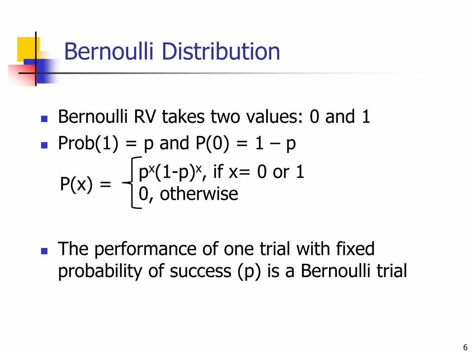
Bernoulli Distribution
Bernoulli RV takes two values: 0 and 1
Prob(1) = p and P(0) = 1 – p
The performance of one trial with fixed probability of success (p) is a Bernoulli trial
6
px(1-p)x, if x= 0 or 10, otherwise
P(x) =

Binomial Distribution
Like Bernoulli distribution, two values: 0 or 1 and probability P(1)=p and P(0)=1-p
What is the probability of k successes, P(k), in a series of n independent trials? (n>=k)
P(k) is a binomial random variable:
Bernoulli distribution is a special case of the binomial distribution (i.e., n=1)
7
pk(1-p)n-k , where = P(x) = nk
nk
n!
k!(n-k)!
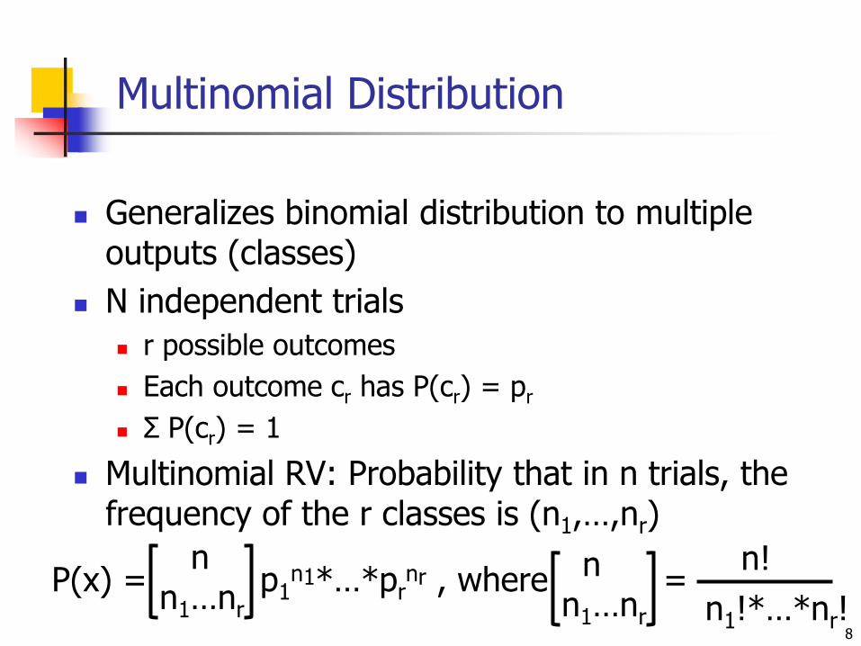
Multinomial Distribution
Generalizes binomial distribution to multiple outputs (classes)
N independent trials
r possible outcomes
Each outcome cr has P(cr) = pr
Σ P(cr) = 1
Multinomial RV: Probability that in n trials, the frequency of the r classes is (n1,…,nr)
8
p1n1*…*pr
nr , where = P(x) = n
n1…nr
n!
n1!*…*nr!
nn1…nr
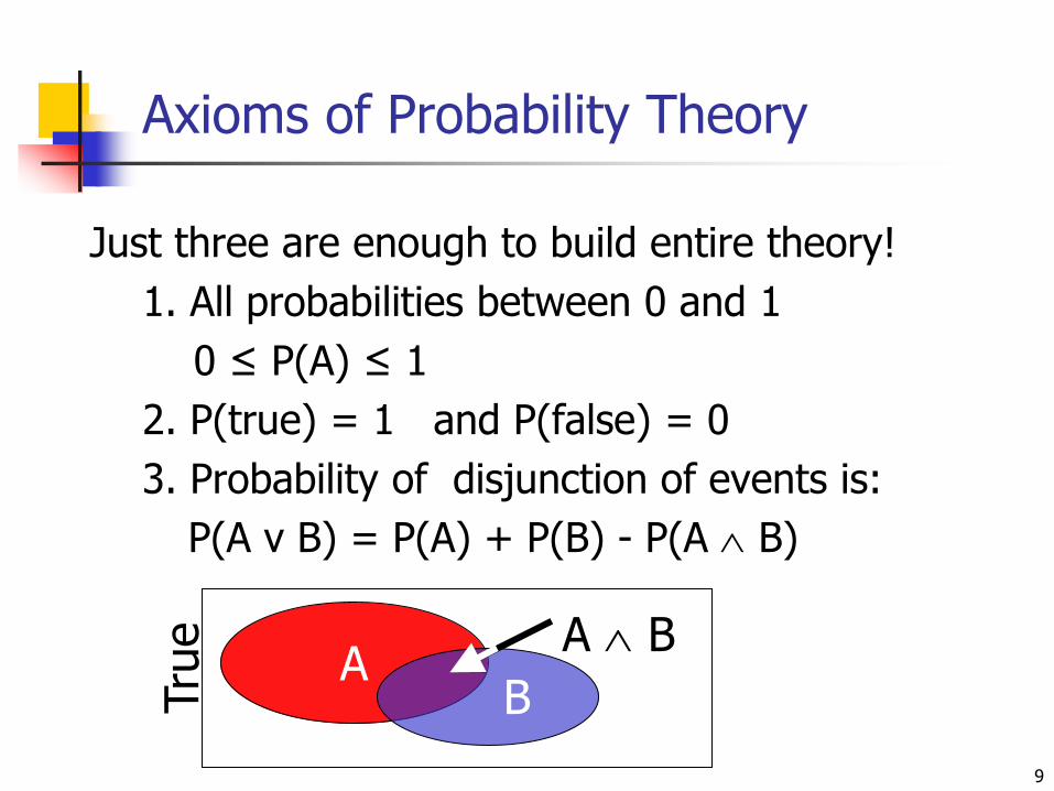
Axioms of Probability Theory
Just three are enough to build entire theory!
1. All probabilities between 0 and 1
0 ≤ P(A) ≤ 1
2. P(true) = 1 and P(false) = 0
3. Probability of disjunction of events is:
P(A v B) = P(A) + P(B) - P(A B)
9
AB
A B
Tru
e
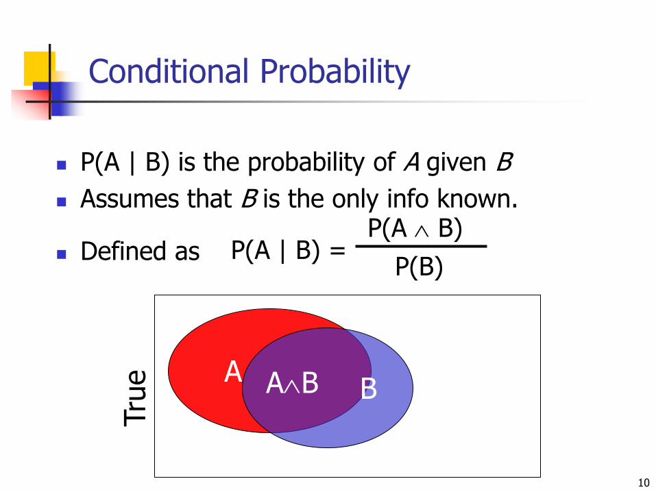
Conditional Probability
P(A | B) is the probability of A given B
Assumes that B is the only info known.
Defined as
10
P(A | B) =P(A B)
P(B)
A BAB
Tru
e
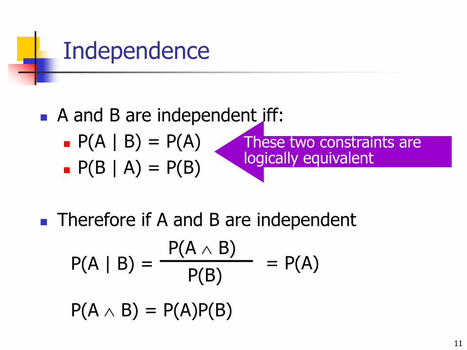
Independence
A and B are independent iff:
P(A | B) = P(A)
P(B | A) = P(B)
Therefore if A and B are independent
11
These two constraints are logically equivalent
P(A | B) =P(A B)
P(B)= P(A)
P(A B) = P(A)P(B)

Independence
12
Tru
e
B
A A B
Independence is powerful, but rarely holds

Conditional Independence
13
Tru
e
B
A A B
A&B not independent,
since P(A|B) < P(A)
14
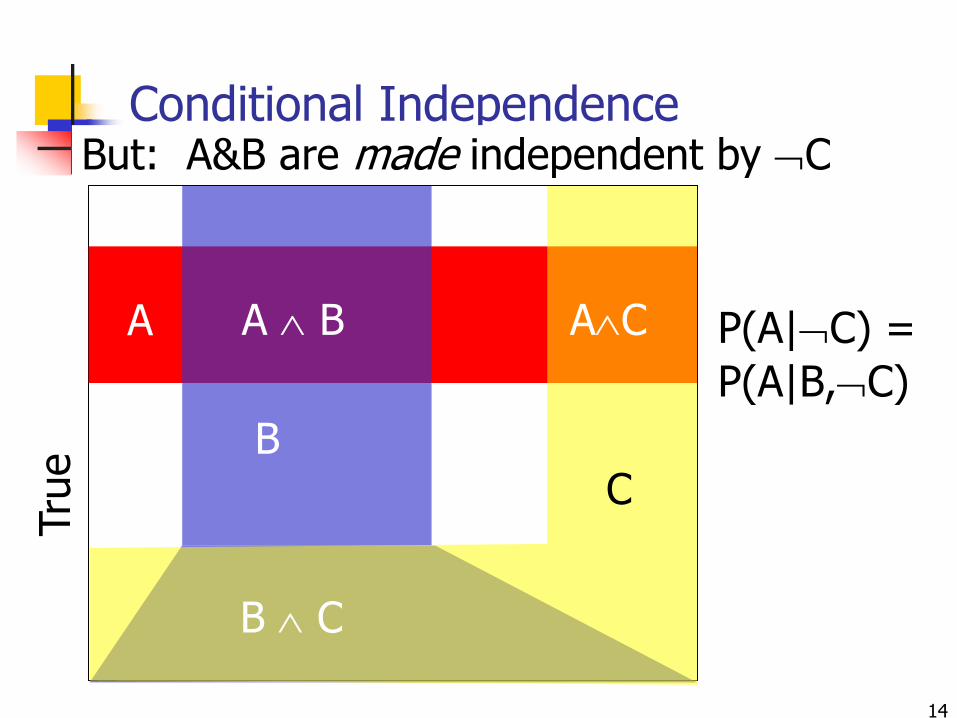
Conditional IndependenceTru
e
B
A A B
C
B C
AC
But: A&B are made independent by C
P(A|C) =
P(A|B,C)
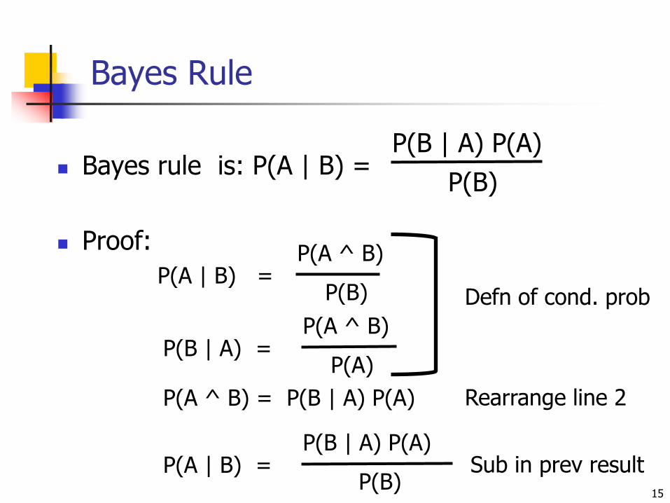
Bayes Rule
Bayes rule is:
Proof:
15
P(A | B) =P(B | A) P(A)
P(B)
P(A | B) =P(B | A) P(A)
P(B)Sub in prev result
P(A ^ B) = P(B | A) P(A) Rearrange line 2
P(A | B) =P(A ^ B)
P(B)
P(B | A) =P(A ^ B)
P(A)
Defn of cond. prob
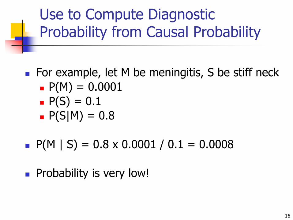
Use to Compute Diagnostic Probability from Causal Probability
For example, let M be meningitis, S be stiff neck
P(M) = 0.0001
P(S) = 0.1
P(S|M) = 0.8
P(M | S) = 0.8 x 0.0001 / 0.1 = 0.0008
Probability is very low!
16

Outline
Probability overview
Naïve Bayes
Bayesian learning
Bayesian networks
17
© Jude Shavlik 2006David Page 2007 Lecture #5, Slide 18
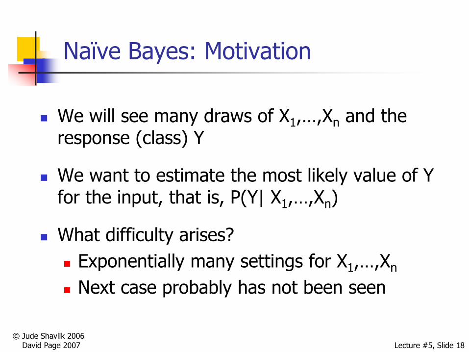
Naïve Bayes: Motivation
We will see many draws of X1,…,Xn and the response (class) Y
We want to estimate the most likely value of Y for the input, that is, P(Y| X1,…,Xn)
What difficulty arises?
Exponentially many settings for X1,…,Xn
Next case probably has not been seen
© Jude Shavlik 2006David Page 2007
CS 760 – Machine Learning (UW-Madison) Lecture #5, Slide 19
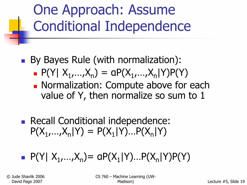
One Approach: Assume Conditional Independence
By Bayes Rule (with normalization):
P(Y| X1,…,Xn) = αP(X1,…,Xn|Y)P(Y)
Normalization: Compute above for each value of Y, then normalize so sum to 1
Recall Conditional independence:P(X1,…,Xn|Y) = P(X1|Y)…P(Xn|Y)
P(Y| X1,…,Xn)= αP(X1|Y)…P(Xn|Y)P(Y)
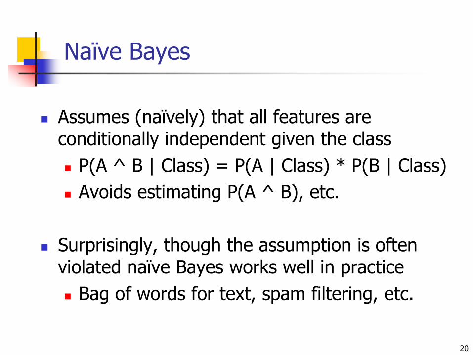
Naïve Bayes
Assumes (naïvely) that all features are conditionally independent given the class
P(A ^ B | Class) = P(A | Class) * P(B | Class)
Avoids estimating P(A ^ B), etc.
Surprisingly, though the assumption is often violated naïve Bayes works well in practice
Bag of words for text, spam filtering, etc.
20
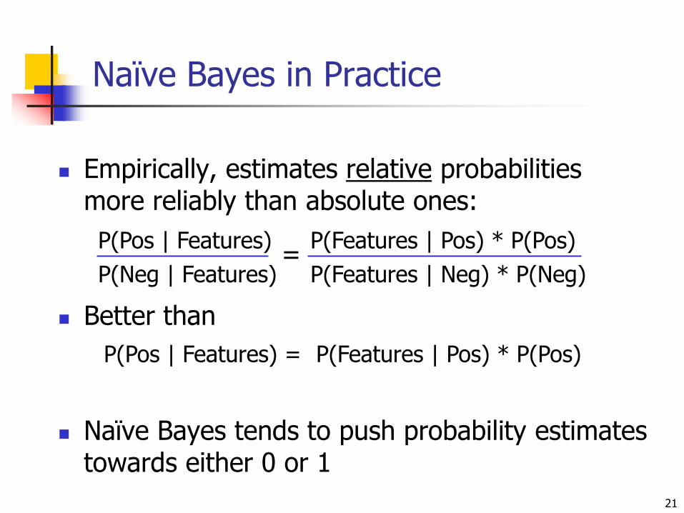
Naïve Bayes in Practice
Empirically, estimates relative probabilities more reliably than absolute ones:
Better than
Naïve Bayes tends to push probability estimates towards either 0 or 1
21
P(Pos | Features) P(Features | Pos) * P(Pos)
P(Neg | Features) P(Features | Neg) * P(Neg) =
P(Pos | Features) = P(Features | Pos) * P(Pos)

Technical Detail: Underflow
Assume we have 100 features
We multiple 100 numbers in [0,1]
If values are small, we are likely to „underflow‟ the min positive/float value
Solution: ∏ probs = e
Sum log‟s of prob‟s
Subtract logs since log = logP(+) – logP(-)
22
P(+)
P(-)
Σ log(prob)

Log Odds
23
P(F1 | Pos)*…* P(Fn | Pos) * P(Pos)
P(F1 | Neg)*…* P(Fn | Neg) * P(Neg) Odds =
log(Odds) = [∑ log{ P(Fi | Pos) / P(Fi | Neg)}]+ log( P(Pos) / P(Neg) )
Notice if a feature value is more likely in a pos, the log is pos and if more likely in neg, the log is neg (0 if tie)
© Jude Shavlik 2006David Page 2007
CS 760 – Machine Learning (UW-Madison) Lecture #5, Slide 24
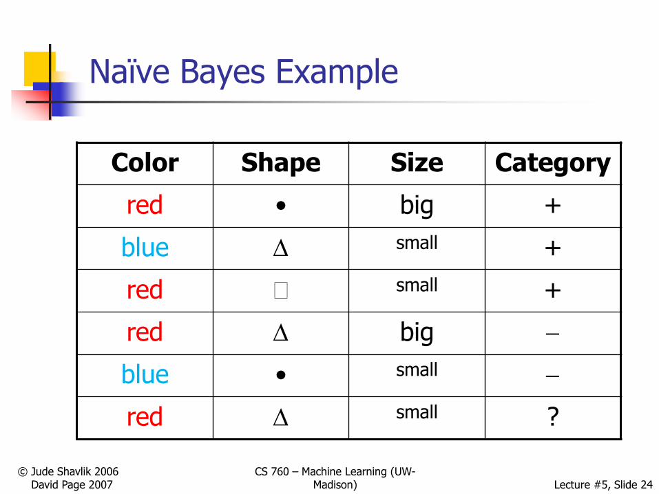
Naïve Bayes Example
Color Shape Size Category
red • big +
blue small +
red small +
red big
blue • small
red small ?
© Jude Shavlik 2006David Page 2007
CS 760 – Machine Learning (UW-Madison) Lecture #5, Slide 25
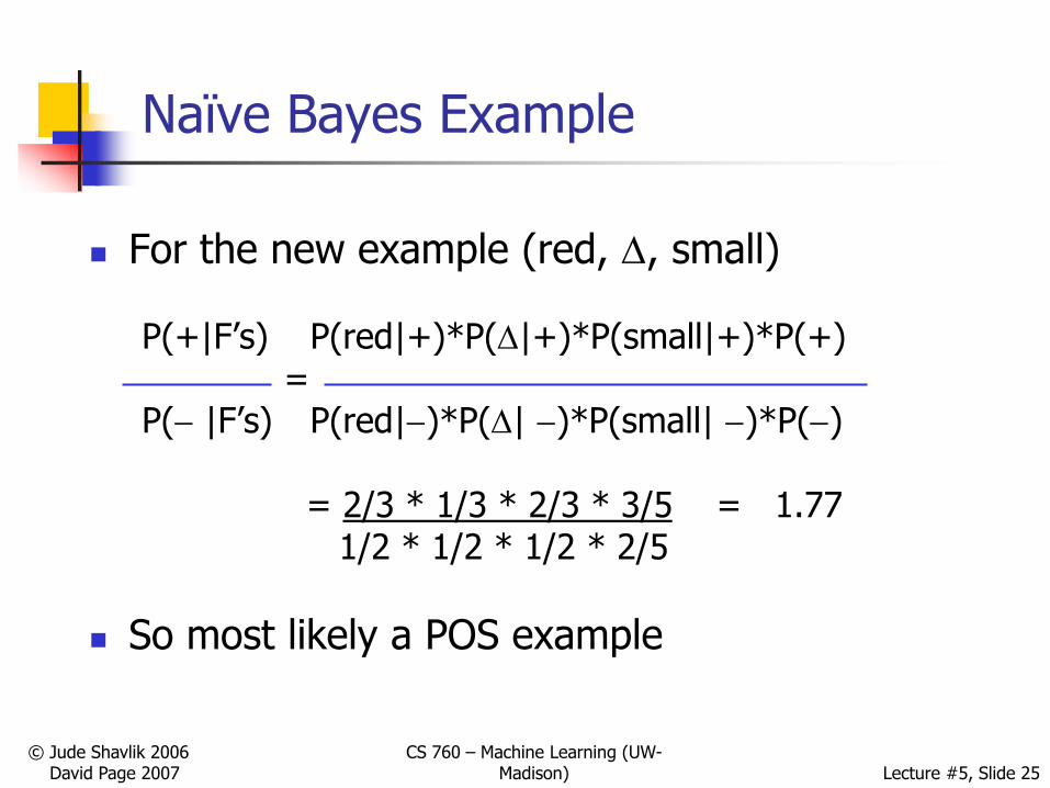
Naïve Bayes Example
For the new example (red, , small)
P(+|F‟s) P(red|+)*P(|+)*P(small|+)*P(+)=
P( |F‟s) P(red|)*P(| )*P(small| )*P()
= 2/3 * 1/3 * 2/3 * 3/5 = 1.771/2 * 1/2 * 1/2 * 2/5
So most likely a POS example

© Jude Shavlik 2006David Page 2007
CS 760 – Machine Learning (UW-Madison) Lecture #5, Slide 26
Dealing with Zeroes (and Small Samples)
If we never see something (eg, in the train set), should we assume its probability is zero?
If we only see 3 pos ex‟s and 2 are red, do we really think
P(red|pos) = 2/3 ?
© Jude Shavlik 2006David Page 2007
CS 760 – Machine Learning (UW-Madison) Lecture #5, Slide 27
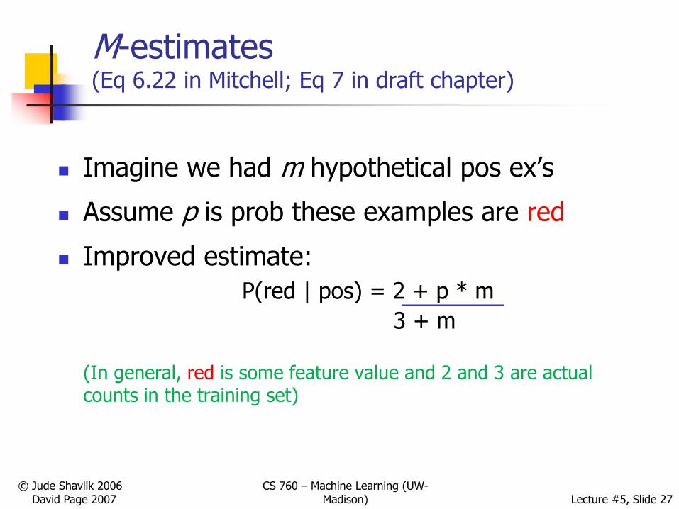
M-estimates (Eq 6.22 in Mitchell; Eq 7 in draft chapter)
Imagine we had m hypothetical pos ex‟s
Assume p is prob these examples are red
Improved estimate:
P(red | pos) = 2 + p * m
3 + m
(In general, red is some feature value and 2 and 3 are actual counts in the training set)
© Jude Shavlik 2006David Page 2007
CS 760 – Machine Learning (UW-Madison) Lecture #5, Slide 28
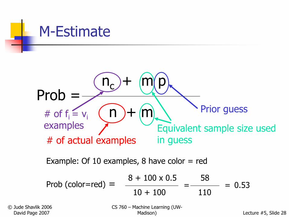
M-Estimate
Prob =nc + m p
n + m
# of actual examples
# of fi = vi
examples Equivalent sample size used in guess
Prior guess
Prob (color=red) =8 + 100 x 0.5
10 + 100=
58
110= 0.53
Example: Of 10 examples, 8 have color = red
© Jude Shavlik 2006David Page 2007
CS 760 – Machine Learning (UW-Madison) Lecture #5, Slide 29
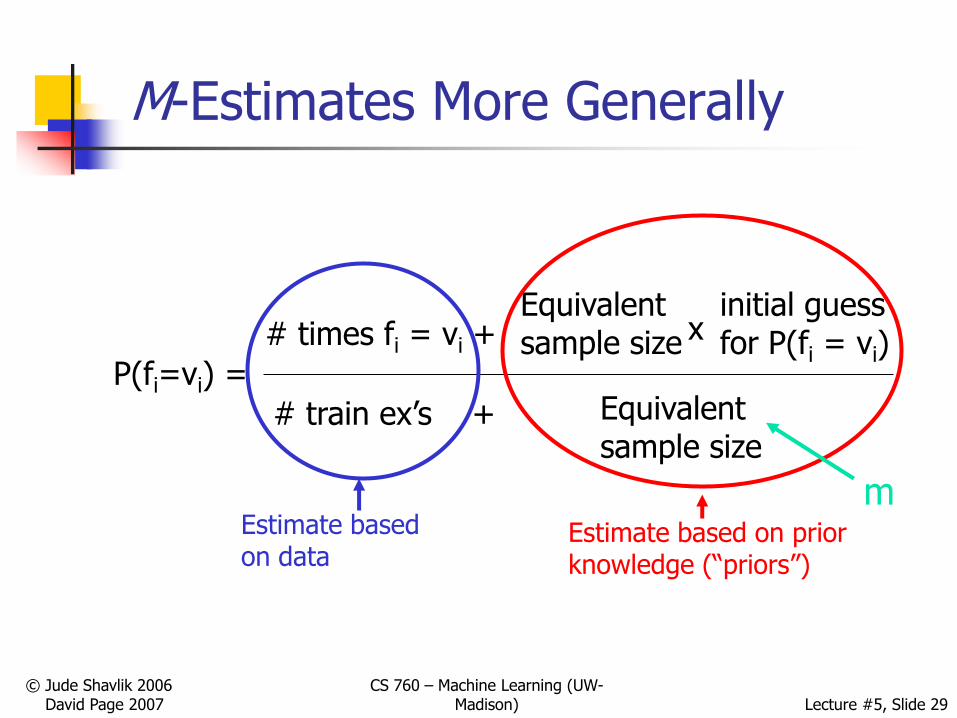
M-Estimates More Generally
P(fi=vi) =
# times fi = vi +Equivalent sample size
# train ex‟s + Equivalent sample size
initial guess for P(fi = vi)
x
Estimate based on prior knowledge (“priors”)
Estimate based on data
m

© Jude Shavlik 2006David Page 2007
CS 760 – Machine Learning (UW-Madison) Lecture #5, Slide 30
Laplace Smoothing
Special case of m estimates Let m = #colors, p = 1/m Ie, assume one hypothetical pos ex of each color
Implementation trick Start all counters at 1 instead of 0
Eg, initialize count(pos, feature(i), value(i, j)) = 1 count(pos, color, red),
count(neg, color, red),count(pos, color, blue), …

Naïve Bayes as a Graphical Model
F2 FN-2 F N-1 FNF1 F3
ClassValue
…
Node i stores P(Fi | POS) and P(Fi | NEG)
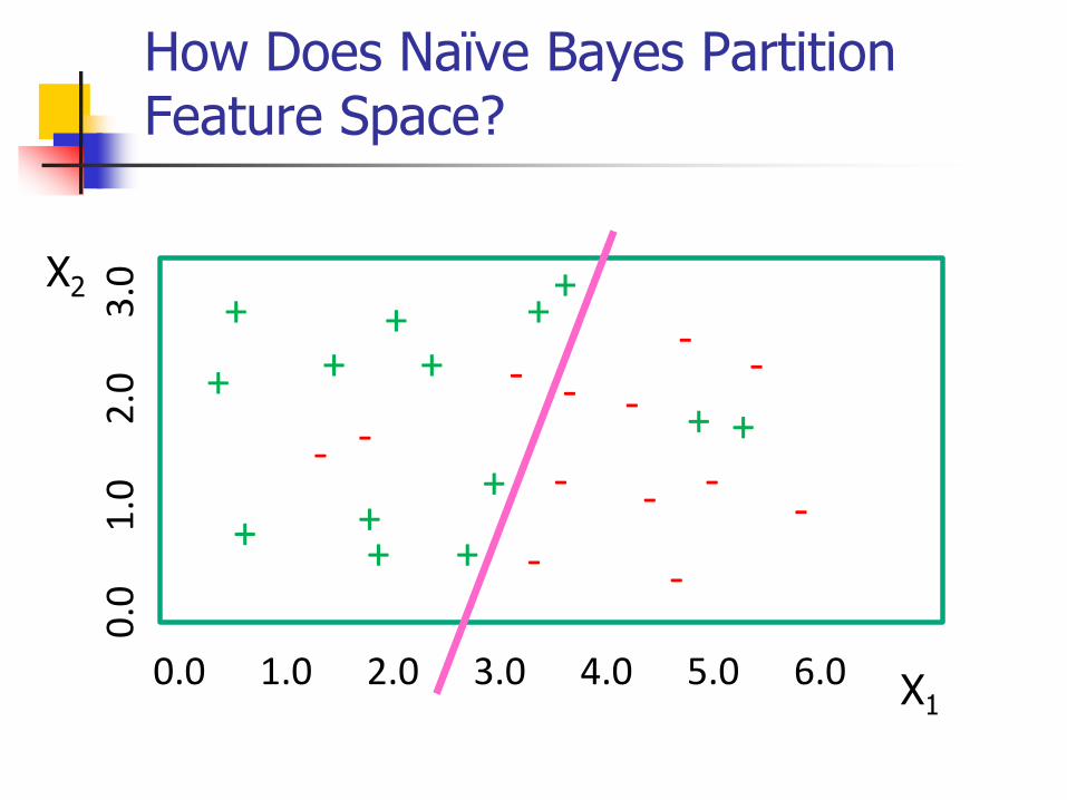
How Does Naïve Bayes Partition Feature Space?
++ ++
- -
-
- -
--
-
-
-
+ ++
+
+
++
-
-
-
+
+
+
0.0 1.0 2.0 3.0 4.0 5.0 6.0
0.0
1.0
2.0
3.0X2
X1
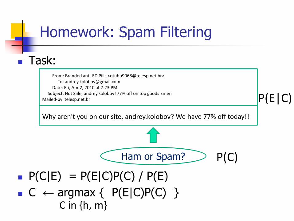
Homework: Spam Filtering
Task:
P(C|E) = P(E|C)P(C) / P(E)
C ← argmax { P(E|C)P(C) }
From: Branded anti-ED Pills <[email protected]>To: [email protected]
Date: Fri, Apr 2, 2010 at 7:23 PMSubject: Hot Sale, andrey.kolobov! 77% off on top goods Emen
Mailed-by: telesp.net.br
Why aren't you on our site, andrey.kolobov? We have 77% off today!!
Ham or Spam?
C in {h, m}
P(C)
P(E|C)

C ← argmax {P(E|C)P(C)} = argmax {P(C) ∏ P(W |C)}
… with Naïve Bayes
From: Branded anti-ED Pills <[email protected]>To: [email protected]
Date: Fri, Apr 2, 2010 at 7:23 PMSubject: Hot Sale, andrey.kolobov! 77% off on top goods Emen
Mailed-by: telesp.net.br
Why aren't you on our site , andrey.kolobov ?We have 77% off today!!
Ham or Spam?
C in {h, m}
P(C)
P(“why”|C) P(“today”|C)
W in E C in {h, m}
P(E|C)
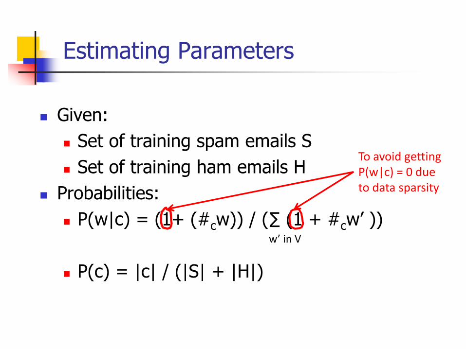
Estimating Parameters
Given:
Set of training spam emails S
Set of training ham emails H
Probabilities:
P(w|c) = (1+ (#cw)) / (∑ (1 + #cw‟ ))
P(c) = |c| / (|S| + |H|)
w’ in V
To avoid getting P(w|c) = 0 due to data sparsity
Naïve Bayes Summary
Fast, simple algorithm
Effective in practice [good baseline comparison]
Gives estimates of confidence in class label
Makes simplifying assumptions
Extensions to come…
36
Outline
Probability overview
Naïve Bayes
Bayesian learning
Bayesian networks
37
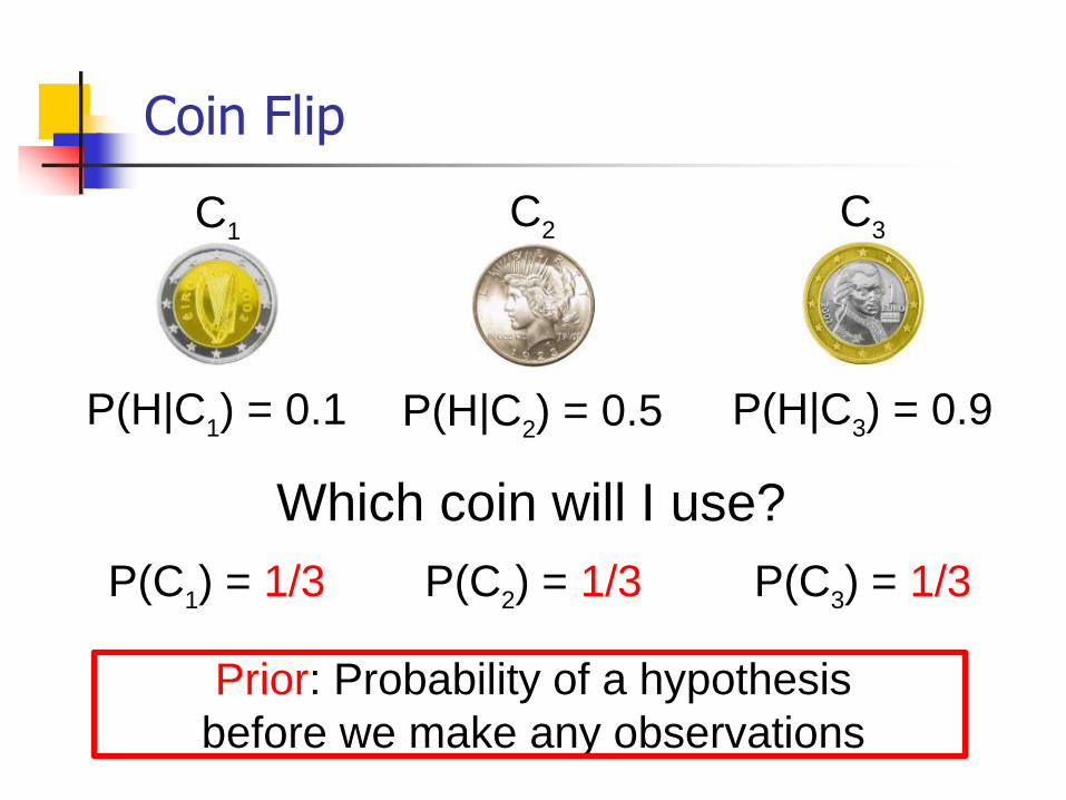
Coin Flip
P(H|C2) = 0.5P(H|C
1) = 0.1
C1
C2
P(H|C3) = 0.9
C3
Which coin will I use?
P(C1) = 1/3 P(C
2) = 1/3 P(C
3) = 1/3
Prior: Probability of a hypothesis
before we make any observations
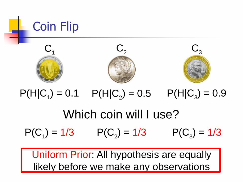
Coin Flip
P(H|C2) = 0.5P(H|C
1) = 0.1
C1
C2
P(H|C3) = 0.9
C3
P(C1) = 1/3 P(C
2) = 1/3 P(C
3) = 1/3
Uniform Prior: All hypothesis are equally
likely before we make any observations
Which coin will I use?
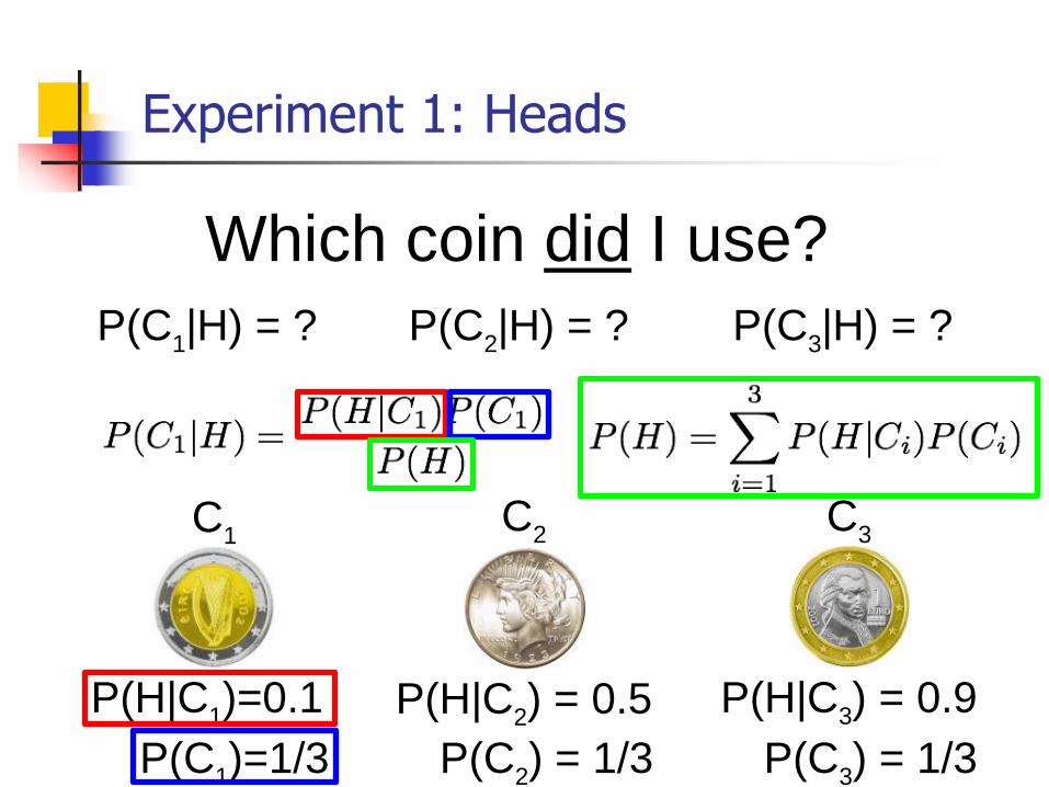
Experiment 1: Heads
Which coin did I use?
P(C1|H) = ? P(C
2|H) = ? P(C
3|H) = ?
P(H|C2) = 0.5 P(H|C
3) = 0.9P(H|C
1)=0.1
C1
C2
C3
P(C1)=1/3 P(C
2) = 1/3 P(C
3) = 1/3

Experiment 1: Heads
Which coin did I use?
P(C1|H) = 0.066 P(C
2|H) = 0.333 P(C
3|H) = 0.6
P(H|C2) = 0.5 P(H|C
3) = 0.9P(H|C
1) = 0.1
C1
C2
C3
P(C1) = 1/3 P(C
2) = 1/3 P(C
3) = 1/3
Posterior: Probability of a hypothesis given data
Terminology
Prior: Probability of a hypothesis before we see any data
Uniform prior: A prior that makes all hypothesis equally likely
Posterior: Probability of hypothesis after we saw some data
Likelihood: Probability of the data given the hypothesis
42

Experiment 2: Tails
Which coin did I use?
P(H|C2) = 0.5 P(H|C
3) = 0.9P(H|C
1) = 0.1
C1
C2
C3
P(C1) = 1/3 P(C
2) = 1/3 P(C
3) = 1/3
P(C1|HT) = ? P(C
2|HT) = ? P(C
3|HT) = ?

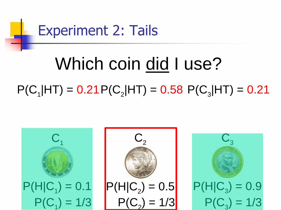
Experiment 2: Tails
Which coin did I use?
P(H|C2) = 0.5 P(H|C
3) = 0.9P(H|C
1) = 0.1
C1
C2
C3
P(C1) = 1/3 P(C
2) = 1/3 P(C
3) = 1/3
P(C1|HT) = 0.21P(C
2|HT) = 0.58 P(C
3|HT) = 0.21
Experiment 2: Tails
Which coin did I use?
P(H|C2) = 0.5 P(H|C
3) = 0.9P(H|C
1) = 0.1
C1
C2
C3
P(C1) = 1/3 P(C
2) = 1/3 P(C
3) = 1/3
P(C1|HT) = 0.21P(C
2|HT) = 0.58 P(C
3|HT) = 0.21
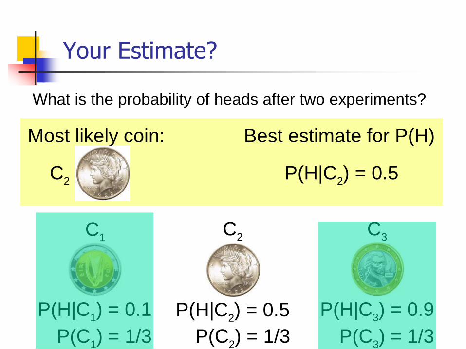
Your Estimate?
What is the probability of heads after two experiments?
P(H|C2) = 0.5 P(H|C
3) = 0.9P(H|C
1) = 0.1
C1
C2
C3
P(C1) = 1/3 P(C
2) = 1/3 P(C
3) = 1/3
Best estimate for P(H)
P(H|C2) = 0.5
Most likely coin:
C2
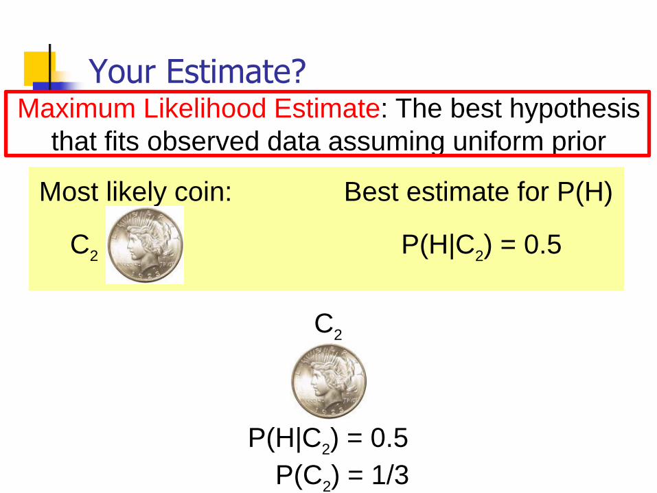
Your Estimate?
P(H|C2) = 0.5
C2
P(C2) = 1/3
Most likely coin: Best estimate for P(H)
P(H|C2) = 0.5C
2
Maximum Likelihood Estimate: The best hypothesis
that fits observed data assuming uniform prior

Using Prior Knowledge
Should we always use a Uniform Prior ?
Background knowledge:
Heads => we have take-home midterm
Jesse likes take-homes…
=> Jesse is more likely to use a coin biased in his favor
P(H|C2) = 0.5P(H|C
1) = 0.1
C1
C2
P(H|C3) = 0.9
C3

Using Prior Knowledge
P(H|C2) = 0.5P(H|C
1) = 0.1
C1
C2
P(H|C3) = 0.9
C3
P(C1) = 0.05 P(C
2) = 0.25 P(C
3) = 0.70
We can encode it in the prior:
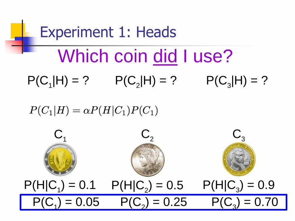
Experiment 1: Heads
Which coin did I use?
P(C1|H) = ? P(C
2|H) = ? P(C
3|H) = ?
P(H|C2) = 0.5 P(H|C
3) = 0.9P(H|C
1) = 0.1
C1
C2
C3
P(C1) = 0.05 P(C
2) = 0.25 P(C
3) = 0.70

Experiment 1: Heads
Which coin did I use?
P(C1|H) = 0.006 P(C
2|H) = 0.165 P(C
3|H) = 0.829
P(H|C2) = 0.5 P(H|C
3) = 0.9P(H|C
1) = 0.1
C1
C2
C3
P(C1) = 0.05 P(C
2) = 0.25 P(C
3) = 0.70
P(C1|H) = 0.066 P(C
2|H) = 0.333 P(C
3|H) = 0.600
Compare with ML posterior after Exp 1:

Experiment 2: Tails
Which coin did I use?
P(C1|HT) = ? P(C
2|HT) = ? P(C
3|HT) = ?
P(H|C2) = 0.5 P(H|C
3) = 0.9P(H|C
1) = 0.1
C1
C2
C3
P(C1) = 0.05 P(C
2) = 0.25 P(C
3) = 0.70
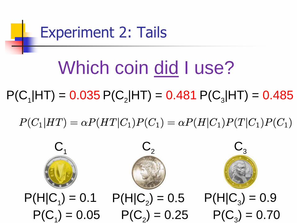
Experiment 2: Tails
Which coin did I use?
P(H|C2) = 0.5 P(H|C
3) = 0.9P(H|C
1) = 0.1
C1
C2
C3
P(C1) = 0.05 P(C
2) = 0.25 P(C
3) = 0.70
P(C1|HT) = 0.035 P(C
2|HT) = 0.481 P(C
3|HT) = 0.485
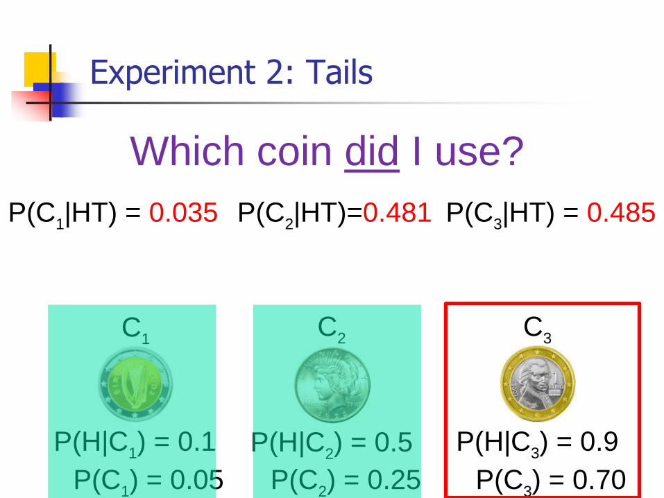
Experiment 2: Tails
Which coin did I use?
P(C1|HT) = 0.035 P(C
2|HT)=0.481 P(C
3|HT) = 0.485
P(H|C2) = 0.5 P(H|C
3) = 0.9P(H|C
1) = 0.1
C1
C2
C3
P(C1) = 0.05 P(C
2) = 0.25 P(C
3) = 0.70
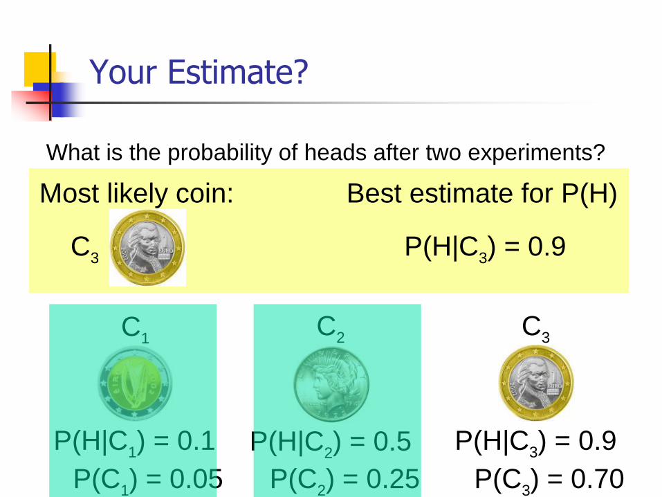
Your Estimate?
What is the probability of heads after two experiments?
P(H|C2) = 0.5 P(H|C
3) = 0.9P(H|C
1) = 0.1
C1
C2
C3
P(C1) = 0.05 P(C
2) = 0.25 P(C
3) = 0.70
Best estimate for P(H)
P(H|C3) = 0.9C
3
Most likely coin:
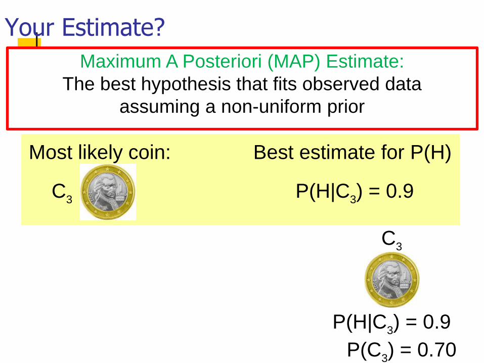
Your Estimate?
Most likely coin: Best estimate for P(H)
P(H|C3) = 0.9C
3
Maximum A Posteriori (MAP) Estimate:
The best hypothesis that fits observed data
assuming a non-uniform prior
P(H|C3) = 0.9
C3
P(C3) = 0.70
Did We Do The Right Thing?
P(H|C2) = 0.5 P(H|C
3) = 0.9P(H|C
1) = 0.1
C1
C2
C3
P(C1|HT)=0.035 P(C
2|HT)=0.481 P(C
3|HT)=0.485
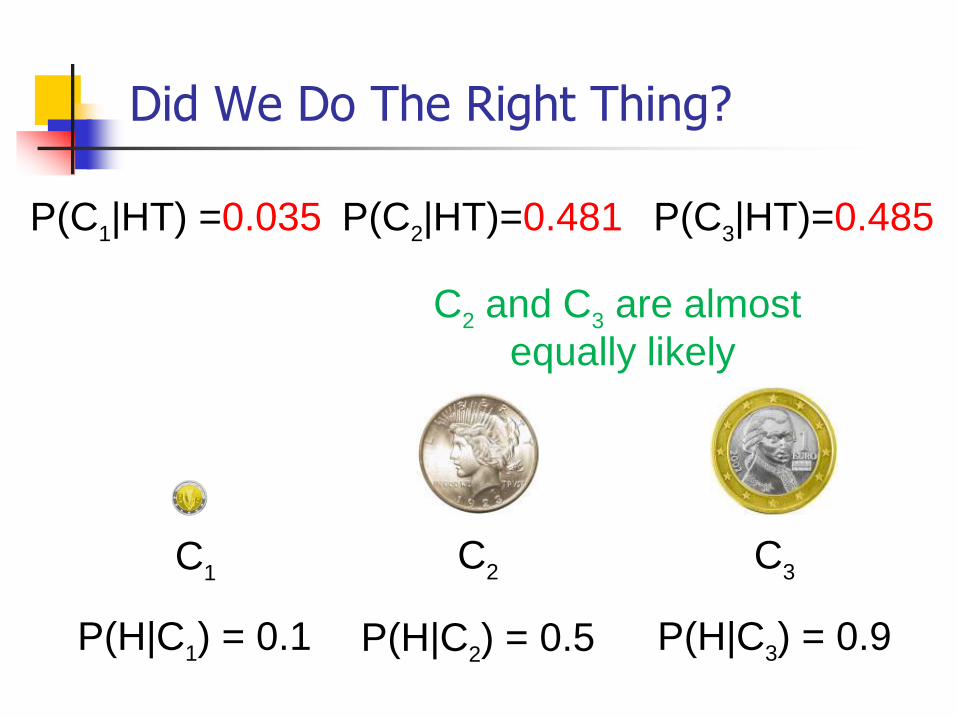
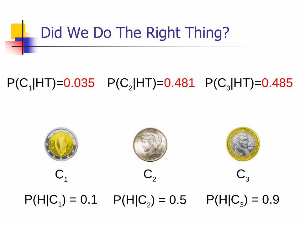
Did We Do The Right Thing?
P(C1|HT) =0.035 P(C
2|HT)=0.481 P(C
3|HT)=0.485
P(H|C2) = 0.5 P(H|C
3) = 0.9P(H|C
1) = 0.1
C1
C2
C3
C2
and C3
are almost
equally likely
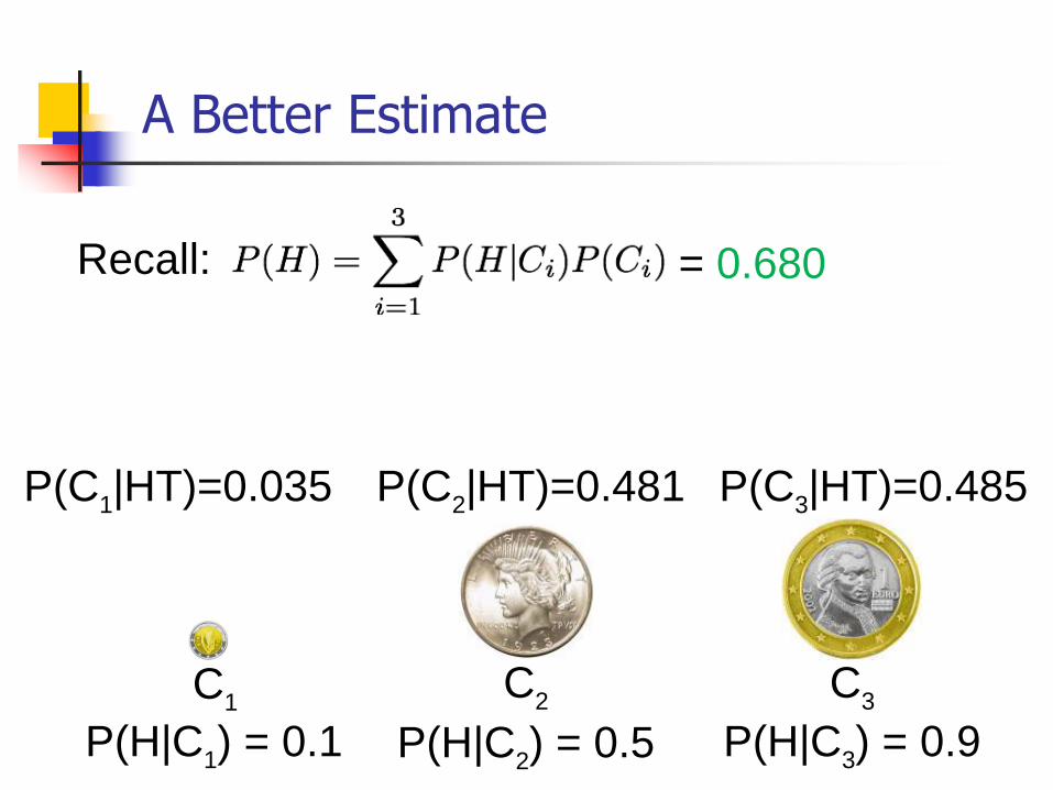
A Better Estimate
P(H|C2) = 0.5 P(H|C
3) = 0.9P(H|C
1) = 0.1
C1
C2
C3
Recall: = 0.680
P(C1|HT)=0.035 P(C
2|HT)=0.481 P(C
3|HT)=0.485

Bayesian Estimate
P(C1|HT)=0.035 P(C
2|HT)=0.481 P(C
3|HT)=0.485
P(H|C2) = 0.5 P(H|C
3) = 0.9P(H|C
1) = 0.1
C1
C2
C3
= 0.680
Bayesian Estimate: Minimizes prediction error,
given data and (generally) assuming a
non-uniform prior
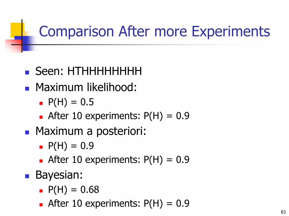
Comparison After more Experiments
Seen: HTHHHHHHHH
Maximum likelihood:
P(H) = 0.5
After 10 experiments: P(H) = 0.9
Maximum a posteriori:
P(H) = 0.9
After 10 experiments: P(H) = 0.9
Bayesian:
P(H) = 0.68
After 10 experiments: P(H) = 0.961
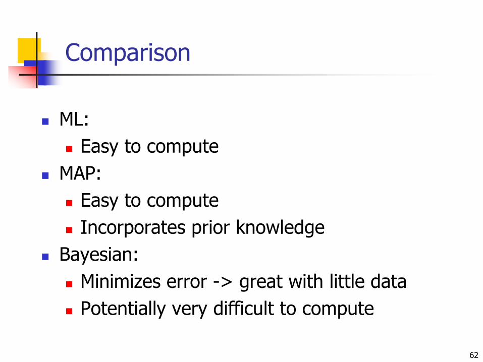
Comparison
ML:
Easy to compute
MAP:
Easy to compute
Incorporates prior knowledge
Bayesian:
Minimizes error -> great with little data
Potentially very difficult to compute
62


Outline
Probability overview
Naïve Bayes
Bayesian learning
Bayesian networks
Representation
Inference
Parameter learning
Structure learning
69
Bayesian Network
In general, a joint distribution P over variables (X1,…,Xn) requires exponential space
A Bayesian network is a graphical representation of the conditional independence relations in P
Usually quite compact
Requires fewer parameters than the full joint distribution
Can yield more efficient inference and belief updates
70
Bayesian Network
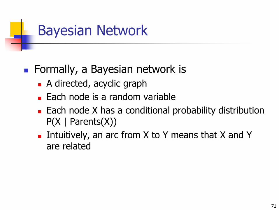
Formally, a Bayesian network is
A directed, acyclic graph
Each node is a random variable
Each node X has a conditional probability distribution P(X | Parents(X))
Intuitively, an arc from X to Y means that X and Y are related
71
© Daniel S. Weld 72
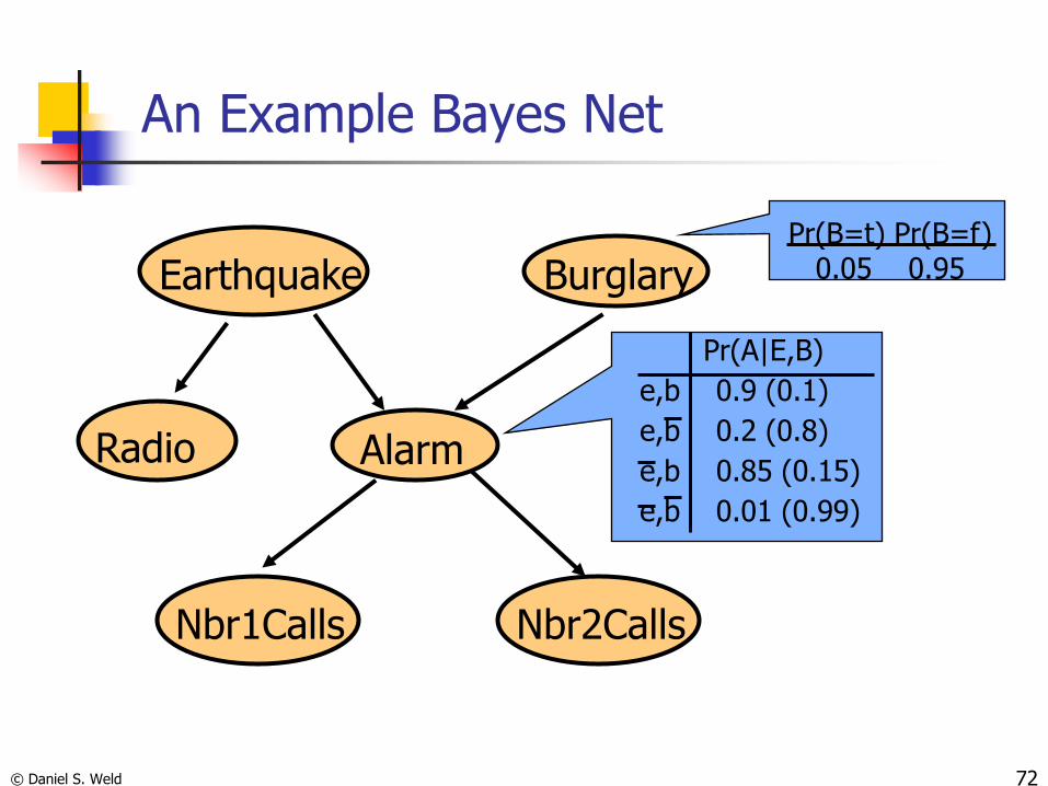
An Example Bayes Net
Earthquake Burglary
Alarm
Nbr2CallsNbr1Calls
Pr(B=t) Pr(B=f)0.05 0.95
Pr(A|E,B)
e,b 0.9 (0.1)
e,b 0.2 (0.8)
e,b 0.85 (0.15)
e,b 0.01 (0.99)
Radio
Terminology
If X and its parents are discrete, we represent P(X|Parents(X)) by
A conditional probability table (CPT)
It specifies the probability of each value of X, given all possible settings for the variables in Parents(X).
Number of parameters locally exponential in |Parents(X)|
A conditioning case is a row in this CPT: A setting of values for the parent nodes
73

Bayesian Network Semantics
A Bayesian network completely specifies a full joint distribution over variables X1,…,Xn
P(x1,…,xn) = ∏ P(xi | Parents(xi))
Here P(x1,…,xn) represents a specific setting for all variables (i.e., P(X1 =x1,…, Xn=xn))
74
i
n
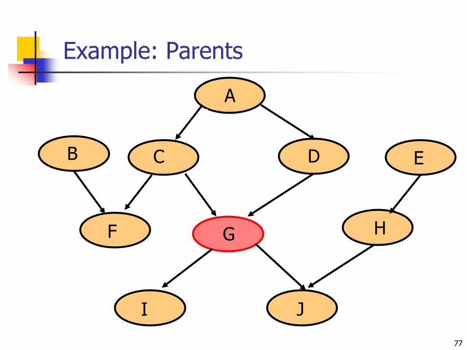
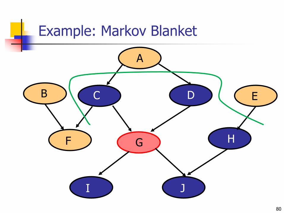
Conditional Indepencies
A node X is conditionally independent of its predecessors given its parents
Markov Blanket of Xi consists of:
Parents of Xi
Children of Xi
Other parents of Xi‟s children
X is conditionally independent of all nodes in the network given its Markov Blanket
75

Example: Parents
76
C D
G
Nbr2CallsNbr1Calls
F
JI
B E
H
AA
Example: Parents
77
C D
G
Nbr2CallsNbr1Calls
F
JI
B E
H
AA
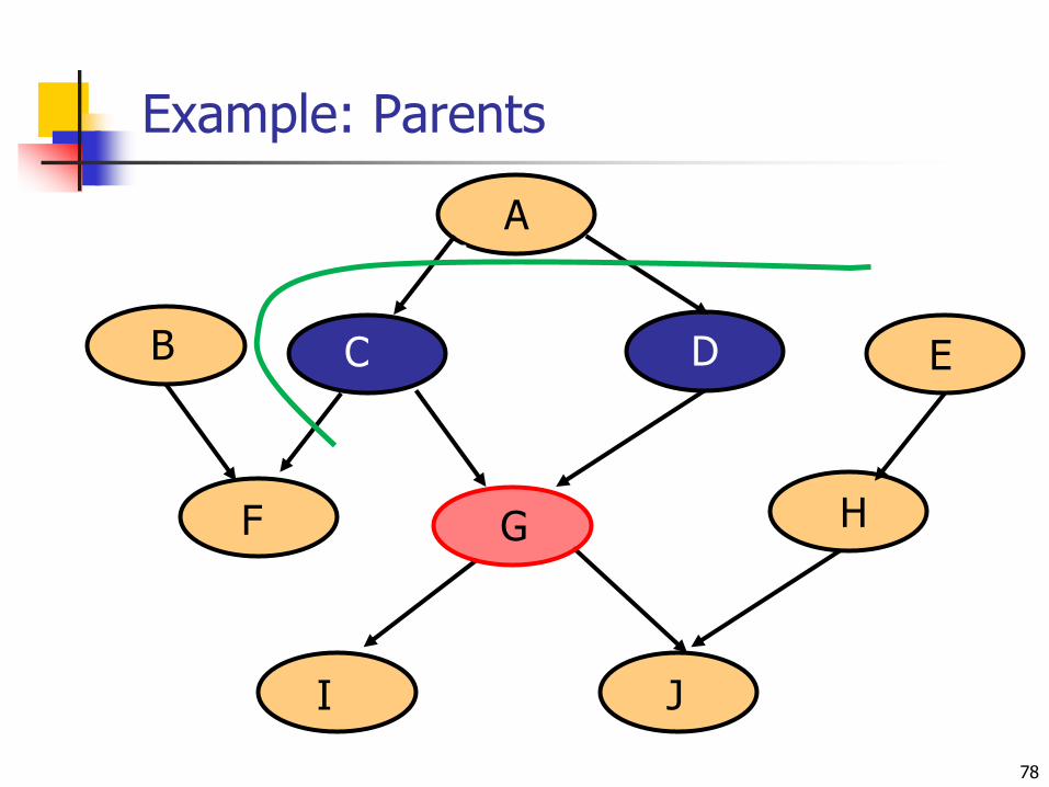
Example: Parents
78
C D
G
Nbr2CallsNbr1Calls
F
JI
B E
H
AA

Example: Markov Blanket
79
C D
G
Nbr2CallsNbr1Calls
F
JI
B E
H
AA
Example: Markov Blanket
80
C D
G
Nbr2CallsNbr1Calls
F
JI
B E
H
AA
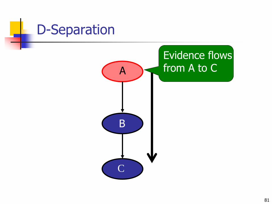
D-Separation
81
C
B
A
Evidence flowsfrom A to C

D-Separation
82
C
A
Evidence flowsfrom A to C
Evidence at B cutsflow from A to CB
D-Separation
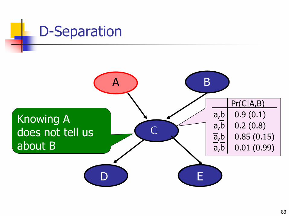
83
C
B
Nbr2CallsNbr1Calls ED
Pr(C|A,B)
a,b 0.9 (0.1)
a,b 0.2 (0.8)
a,b 0.85 (0.15)
a,b 0.01 (0.99)
Knowing Adoes not tell us about B
A
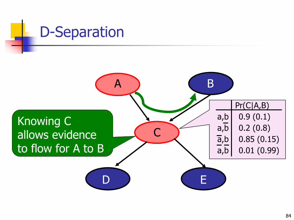
D-Separation
84
A B
C
Nbr2CallsNbr1Calls ED
Pr(C|A,B)
a,b 0.9 (0.1)
a,b 0.2 (0.8)
a,b 0.85 (0.15)
a,b 0.01 (0.99)
Knowing Callows evidenceto flow for A to B
A
D-Separation
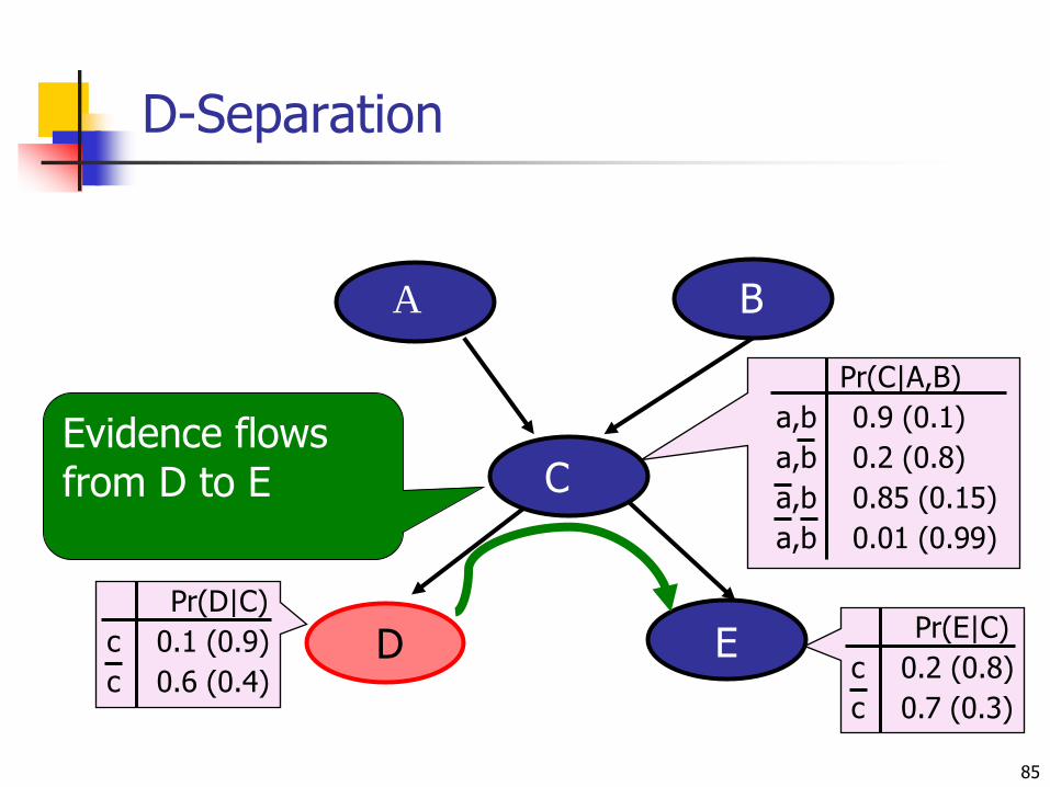
85
A B
Nbr2CallsNbr1Calls ED Pr(E|C)
c 0.2 (0.8)
c 0.7 (0.3)
Pr(D|C)
c 0.1 (0.9)
c 0.6 (0.4)D
CEvidence flowsfrom D to E
Pr(C|A,B)
a,b 0.9 (0.1)
a,b 0.2 (0.8)
a,b 0.85 (0.15)
a,b 0.01 (0.99)
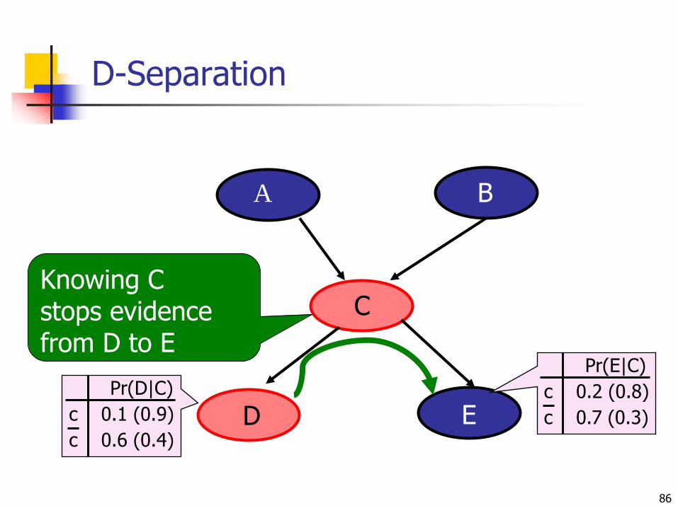
D-Separation
86
A B
C
Nbr2CallsNbr1Calls ED
Pr(E|C)
c 0.2 (0.8)
c 0.7 (0.3)
Knowing Cstops evidencefrom D to E
Pr(D|C)
c 0.1 (0.9)
c 0.6 (0.4)D
Outline
Probability overview
Naïve Bayes
Bayesian learning
Bayesian networks
Representation
Inference
Parameter learning
Structure learning
87
Inference in BNs
The graphical independence representation yields efficient inference schemes
Generally, we want to compute
P(X) or
P(X | E), where E is (conjunctive) evidence
Computations organized by network topology
Two well-known exact algorithms:
Variable elimination
Junction trees88
Variable Elimination
A factor is a function from set of variables to a specific value: CPTS are factors
E.g.: p(A | E,B) is a function of A,E,B
VE works by eliminating all variables in turn until there is a factor with only query variable
89
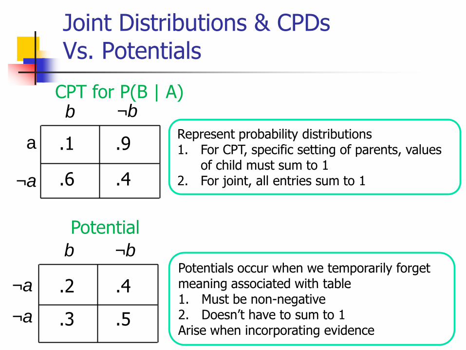
Joint Distributions & CPDs Vs. Potentials
¬b
¬b
¬a
¬a
a
b
¬a
b
.1
.6
.9
.4
.2
.3
.4
.5
CPT for P(B | A)
Potential
Potentials occur when we temporarily forget meaning associated with table1. Must be non-negative2. Doesn‟t have to sum to 1Arise when incorporating evidence
Represent probability distributions1. For CPT, specific setting of parents, values
of child must sum to 12. For joint, all entries sum to 1
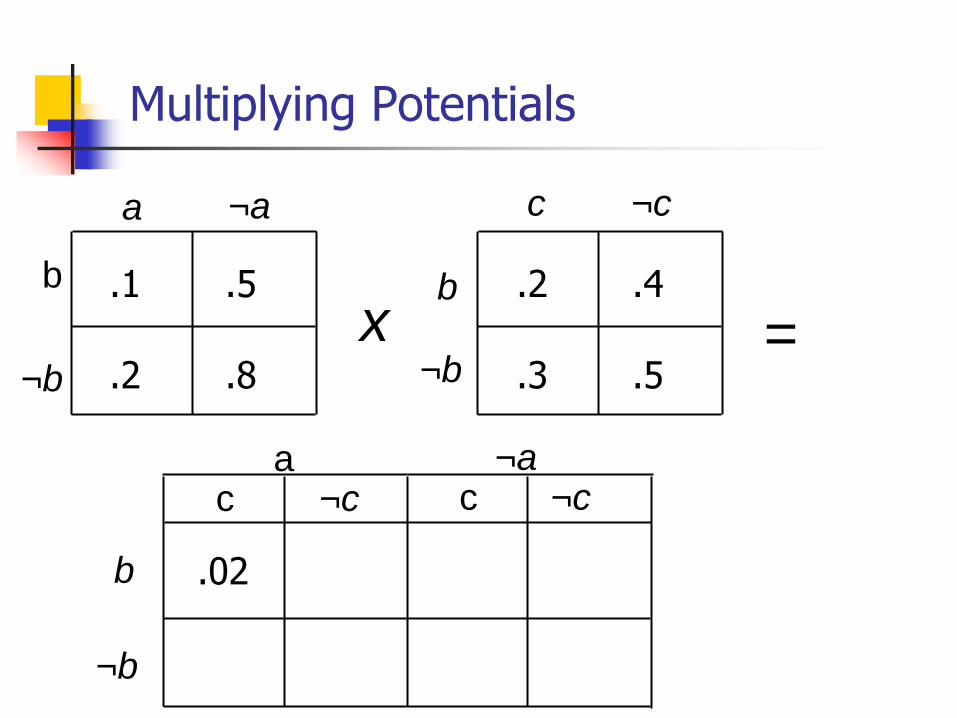
Multiplying Potentials
¬c¬a
¬b ¬b
¬b
¬c ¬ccc
b
b
a
b
c
a ¬a
.1
.2
.5
.8
.2
.3
.4
.5
.02
x =

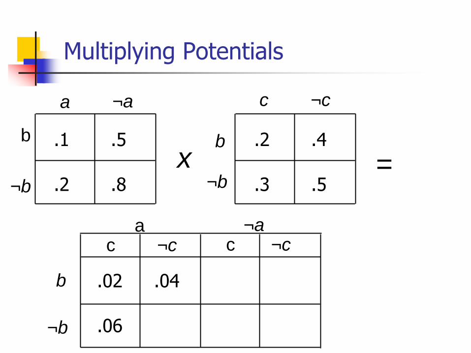
Multiplying Potentials
¬c¬a
¬b ¬b
¬b
¬c ¬ccc
b
b
a
b
c
a ¬a
.1
.2
.5
.8
.2
.3
.4
.5
.02 .04
x =
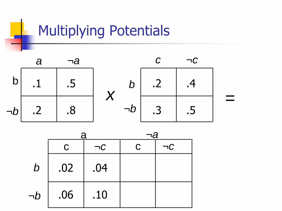
Multiplying Potentials
¬c¬a
¬b ¬b
¬b
¬c ¬ccc
b
b
a
b
c
a ¬a
.1
.2
.5
.8
.2
.3
.4
.5
.02
.06
.04
x =
Multiplying Potentials
¬c¬a
¬b ¬b
¬b
¬c ¬ccc
b
b
a
b
c
a ¬a
.1
.2
.5
.8
.2
.3
.4
.5
.02
.06
.04
.10
x =
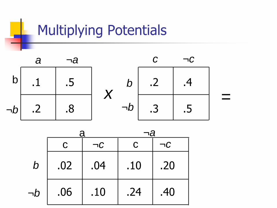
Multiplying Potentials
¬c¬a
¬b ¬b
¬b
¬c ¬ccc
b
b
a
b
c
a ¬a
.1
.2
.5
.8
.2
.3
.4
.5
.10
.24
.20
.40
.02
.06
.04
.10
x =

¬b
¬a
a
b
.1
.2
.5
.8
=
¬b
¬a
a
b
.1
.2
.5
.8
¬b
¬a
a
b
.0625
.125
.3125
.5
a
¬bb
.3 1.3
Marginalize/sum out a variable
Normalize a potential
α

Key Observation
¬b
¬c ¬ccc
b
a ¬a
.04
.24
.08
.40
.02
.06
.04
.25x =
¬a
¬bb
a .1
.2
.5
.8 ¬b
¬cc
b .2
.3
.4
.5
a(P1 x P2) = ( a P1 )x P2 if A is not in P2

Key Observation
¬b
¬c ¬ccc
b
a ¬a
.04
.24
.08
.40
.02
.15
.04
.25x =
¬a
¬bb
a .1
.2
.5
.8 ¬b
¬cc
b .2
.3
.4
.5
¬b
¬cc
b .06
.39
.12
.65x =
¬a
¬bb
a .1
.2
.5
.8 ¬b
¬cc
b .2
.3
.4
.5¬b
b .3
1.3 a
a¬b
¬cc
b .06
.39
.12
.65
a(P1 x P2) = ( a P1 )x P2 if A is not in P2
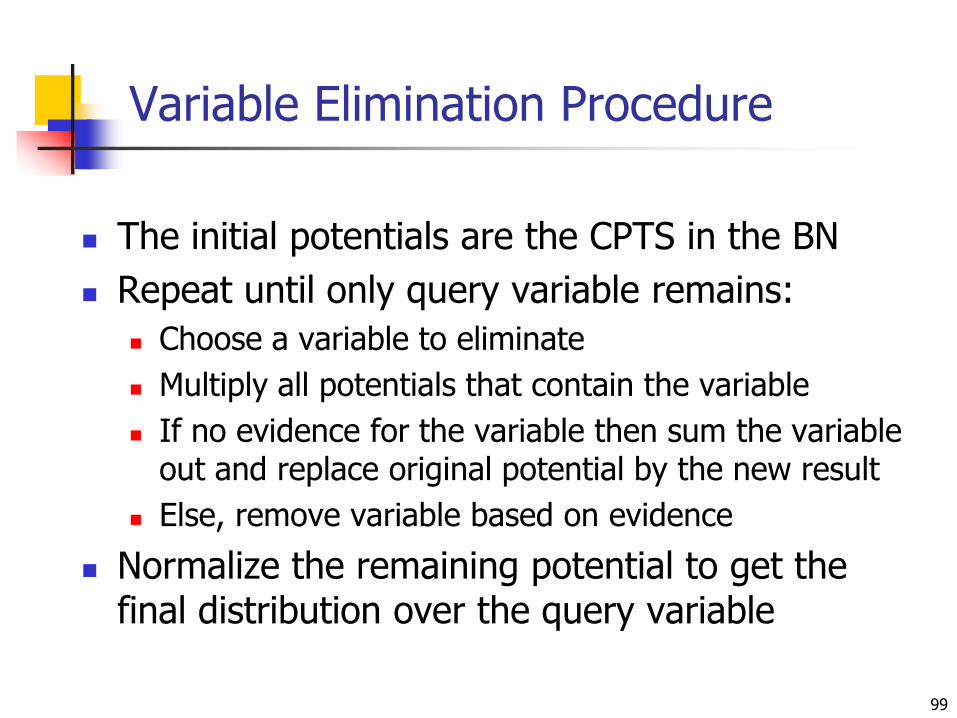
Variable Elimination Procedure
The initial potentials are the CPTS in the BN
Repeat until only query variable remains:
Choose a variable to eliminate
Multiply all potentials that contain the variable
If no evidence for the variable then sum the variable out and replace original potential by the new result
Else, remove variable based on evidence
Normalize the remaining potential to get the final distribution over the query variable
99
A
F
E
C
D
B
¬dd
.1 .3
¬a
a
b
.8
.3
¬b
b
d
.4
.7
¬a
a
c
.1
.6
¬c
c
e
.5
.9
.4 .9
¬ee ¬ee
f
.2
a
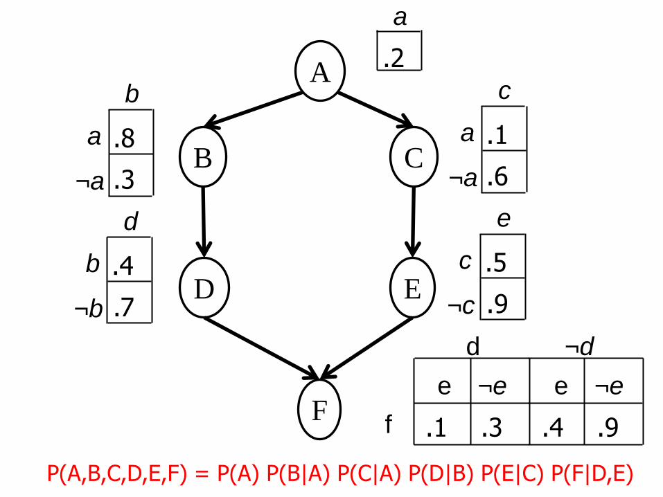
P(A,B,C,D,E,F) = P(A) P(B|A) P(C|A) P(D|B) P(E|C) P(F|D,E)
A
CB¬a
a
c
.1
.6
.2
a
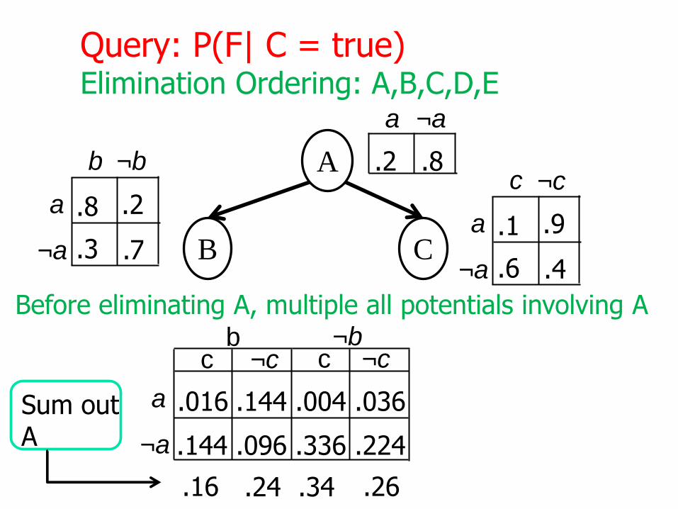
Query: P(F| C = true)Elimination Ordering: A,B,C,D,E
.8
.9
.4¬a
a
b
.8
.3
.2
.7
¬b¬c
¬a
¬a
¬c ¬ccc
a
b ¬b
.004
.336
.036
.224
.016
.144
.144
.096
Before eliminating A, multiple all potentials involving A
.16 .24 .34 .26
Sum outA
D
B C
¬b
¬d ¬ddd
b
c ¬c
.096
.182
.144
.078
.064
.238
.096
.102
.302 .198 .278 .222
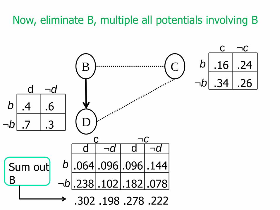
Sum outB
¬b
¬dd
b .4
.7
.6
.3
¬b
¬cc
b .16
.34
.24
.26
Now, eliminate B, multiple all potentials involving B

E
C
D
¬c
¬e ¬eee
c
d ¬d
.099
.200
.099
.022
.151
.250
.151
.028
We have evidence forC, so eliminate ¬c
¬c
¬ee
c .5
.9
.5
.1¬c
¬dd
c .302
.278
.198
.222
Next, eliminate C, multiple all potentials involving C

F
ED
¬f
¬e ¬eee
f
d ¬d
.4
.6
.9
.1
.1
.9
.3
.7
¬d
¬f ¬fff
d
e ¬e
.040
.089
.106
.010
.015
.040
.136
.059
.055 .195 .129 .116
Sum outd
¬e
¬dd
e .151
.151
.099
.099
Next, eliminate D, multiple all potentials involving D
¬e
¬ff
e .055
.129
.195
.116
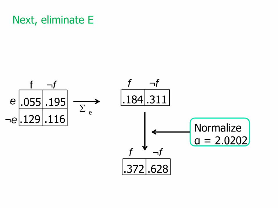
Normalizeα = 2.0202
¬e
¬ff
e .055
.129
.195
.116
Next, eliminate E
.184
f ¬f
.311
.372
f ¬f
.628
e
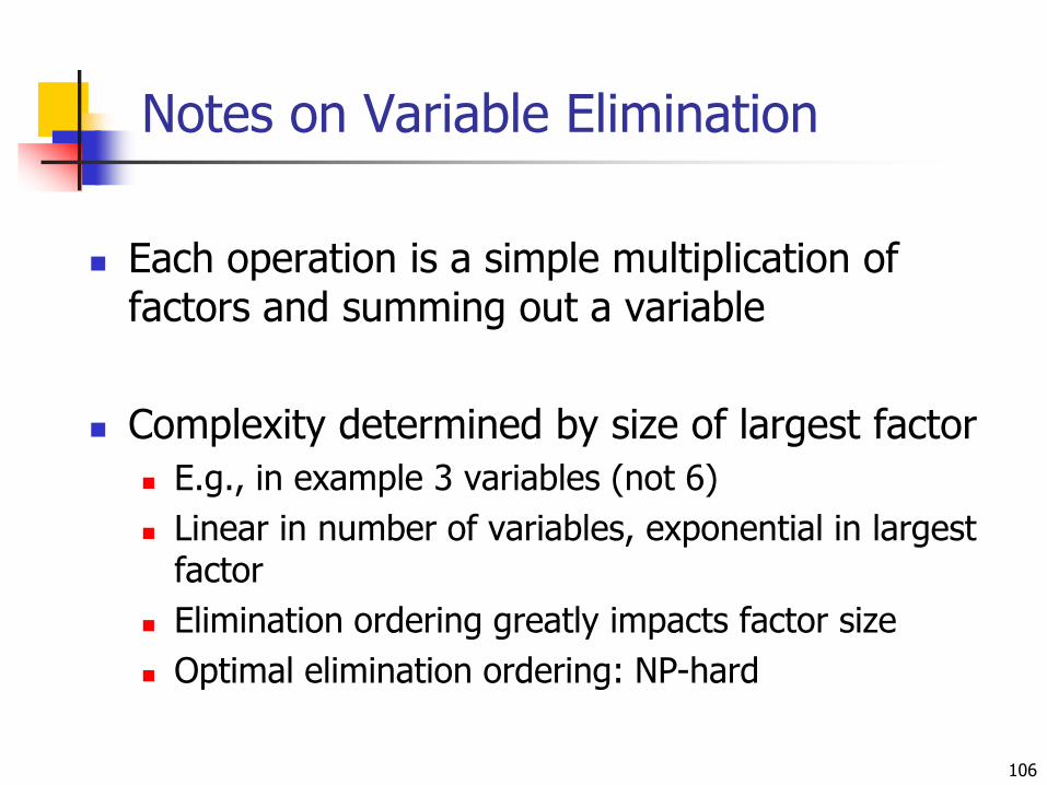
Notes on Variable Elimination
Each operation is a simple multiplication of factors and summing out a variable
Complexity determined by size of largest factor
E.g., in example 3 variables (not 6)
Linear in number of variables, exponential in largest factor
Elimination ordering greatly impacts factor size
Optimal elimination ordering: NP-hard
106
Outline
Probability overview
Naïve Bayes
Bayesian learning
Bayesian networks
Representation
Inference
Parameter learning
Structure learning
107
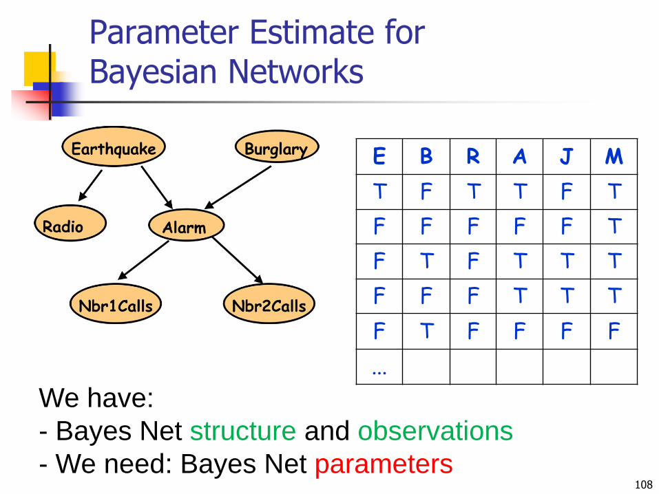
Parameter Estimate for Bayesian Networks
108
E B R A J M
T F T T F T
F F F F F T
F T F T T T
F F F T T T
F T F F F F
...
We have:
- Bayes Net structure and observations
- We need: Bayes Net parameters
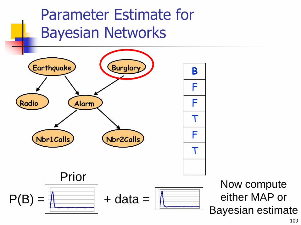
Parameter Estimate for Bayesian Networks
109
P(B) = ?-5
0
5
10
15
20
25
0 0.2 0.4 0.6 0.8 1
Prior
+ data = -2
0
2
4
6
8
10
12
14
16
18
20
0 0.2 0.4 0.6 0.8 1
Now compute
either MAP or
Bayesian estimate
E B R A J M
T F T T F T
F F F F F T
F T F T T T
F F F T T T
F T F F F F
...
What Prior to Use
The following are two common priors
Binary variable Beta
Posterior distribution is binomial
Easy to compute posterior
Discrete variable Dirichlet
Posterior distribution is multinomial
Easy to compute posterior
110
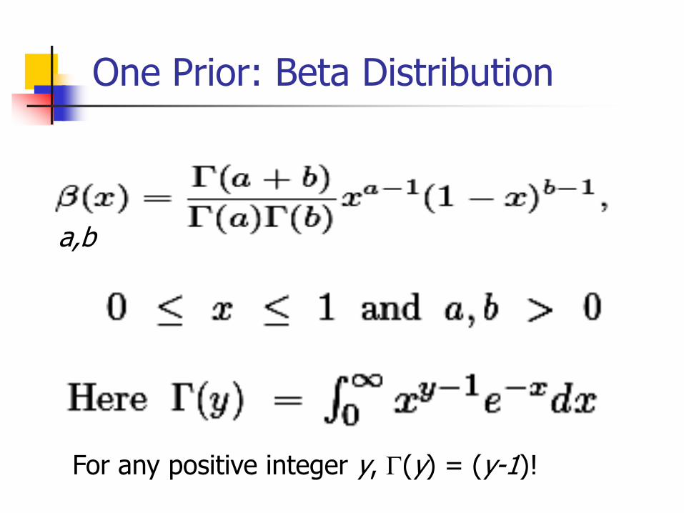
One Prior: Beta Distribution
a,b
For any positive integer y, G(y) = (y-1)!
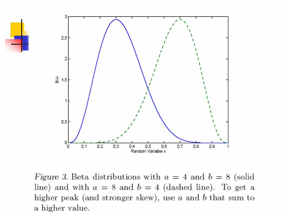

Beta Distribution
Example: Flip coin with Beta distribution as prior p [prob(heads)]
Parameterized by two positive numbers: a and b
Mode of distribution (E[p]) is a /(a+b)
Specify our prior belief for p = a / (a+b)
Specify confidence with initial values of a and b
Updating our prior belief based on data by
Increment a for each head outcome
Increment b for each tail outcome
Posterior is a binomial distribution!113
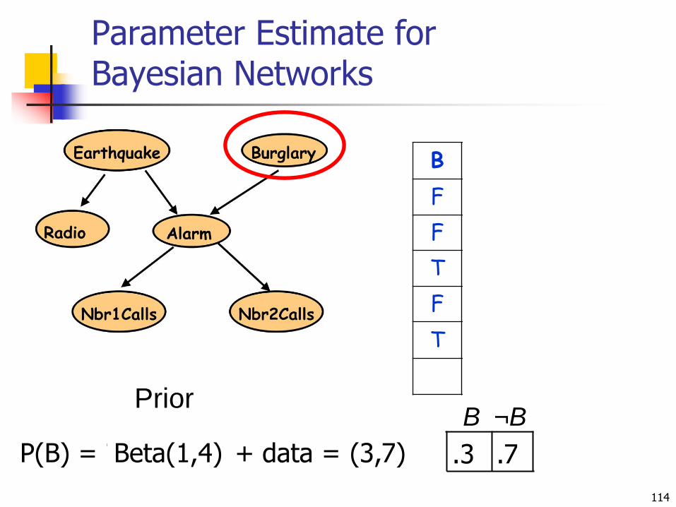
Parameter Estimate for Bayesian Networks
114
E B R A J M
T F T T F T
F F F F F T
F T F T T T
F F F T T T
F T F F F F
...
P(B) = ?
Prior
+ data = Beta(1,4) (3,7) .3
B ¬B
.7

Parameter Estimate for Bayesian Networks
115
E B R A J M
T F T T F T
F F F F F T
F T F T T T
F F F T T T
F T F F F F
...P(A|E,B) = ?
P(A|E,¬B) = ?
P(A|¬E,B) = ?
P(A|¬E,¬B) = ?

Parameter Estimate for Bayesian Networks
116
E B R A J M
T F T T F T
F F F F F T
F T F T T T
F F F T T T
F T F F F F
...P(A|E,B) = ?
P(A|E,¬B) = ?
P(A|¬E,B) = ?
P(A|¬E,¬B) = ?
Prior
Beta(2,3) (3,4)+ data=

© Jude Shavlik 2006David Page 2007 Lecture #5, Slide 117
General EM Framework:Handling Missing Values
Given: Data with missing values, space of possible models, initial model
Repeat until no change greater than threshold:
Expectation (E) Step: Compute expectation over missing values, given model.
Maximization (M) Step: Replace current model with model that maximizes probability of data.

© Jude Shavlik 2006David Page 2007
CS 760 – Machine Learning (UW-Madison) Lecture #5, Slide 118
“Soft” EM vs. “Hard” EM
Soft EM: Expectation is a probability distribution
Hard EM: Expectation is “all or nothing,” assign most likely/probable value
Advantage of hard EM is computational efficiency when expectation is over state consisting of values for multiple variables

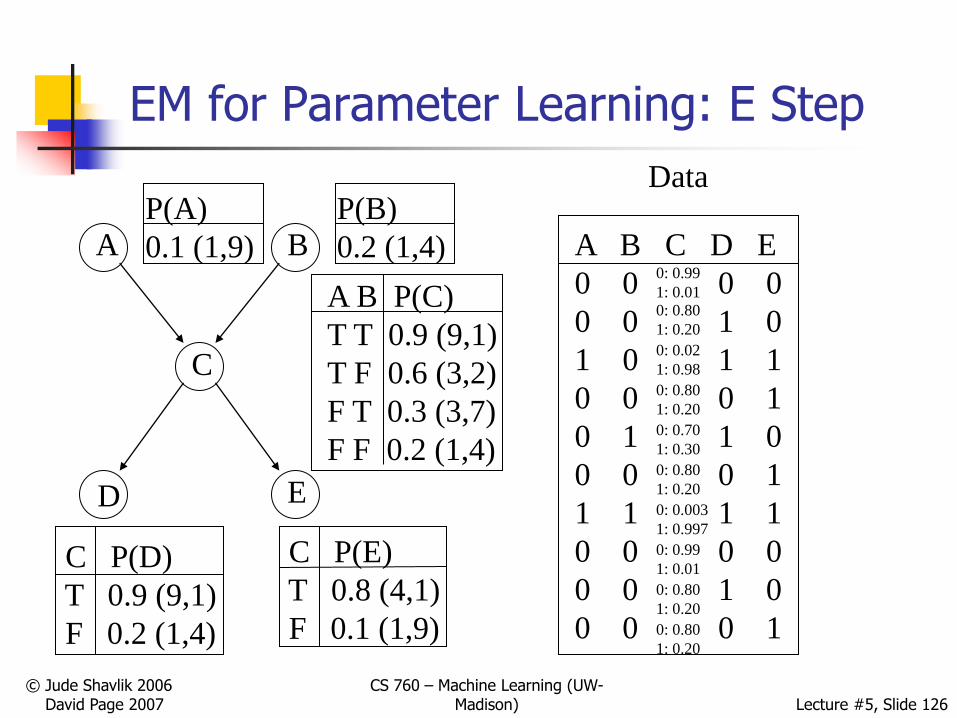
EM for Parameter Learning: E Step
For each data point with missing values
Compute the probability of each possible completion of that data point
Replace the original data point with all completions, weighted by probabilities
Computing the probability of each completion (expectation) is just answering query over missing variables given others
119
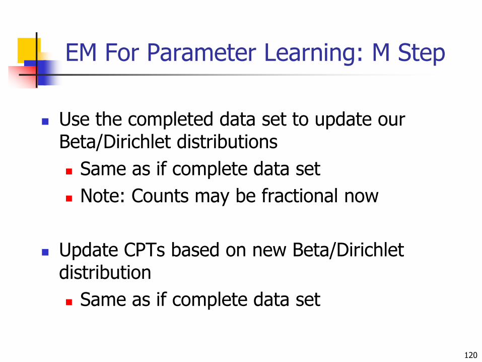
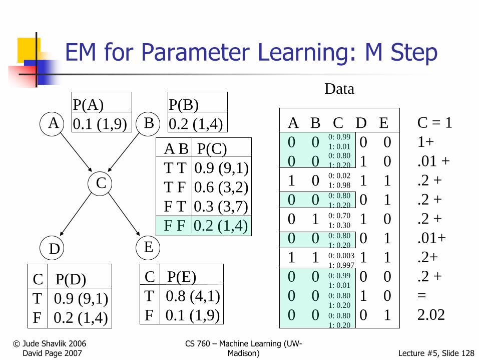
EM For Parameter Learning: M Step
Use the completed data set to update our Beta/Dirichlet distributions
Same as if complete data set
Note: Counts may be fractional now
Update CPTs based on new Beta/Dirichletdistribution
Same as if complete data set
120
© Jude Shavlik 2006David Page 2007
CS 760 – Machine Learning (UW-Madison) Lecture #5, Slide 121
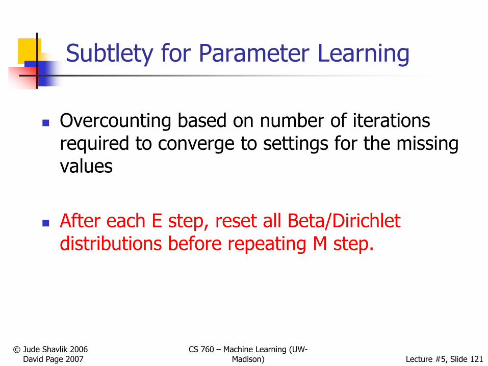
Subtlety for Parameter Learning
Overcounting based on number of iterations required to converge to settings for the missing values
After each E step, reset all Beta/Dirichletdistributions before repeating M step.

© Jude Shavlik 2006David Page 2007
CS 760 – Machine Learning (UW-Madison) Lecture #5, Slide 122
EM for Parameter Learning
C P(D)
T 0.9 (9,1)
F 0.2 (1,4)
A B
C
D E
P(A)
0.1 (1,9)
A B P(C)
T T 0.9 (9,1)
T F 0.6 (3,2)
F T 0.3 (3,7)
F F 0.2 (1,4)
P(B)
0.2 (1,4)
C P(E)
T 0.8 (4,1)
F 0.1 (1,9)
A B C D E
0 0 ? 0 0
0 0 ? 1 0
1 0 ? 1 1
0 0 ? 0 1
0 1 ? 1 0
0 0 ? 0 1
1 1 ? 1 1
0 0 ? 0 0
0 0 ? 1 0
0 0 ? 0 1
Data

Lecture #5, Slide 123
EM for Parameter Learning: E Step
C P(D)
T 0.9 (9,1)
F 0.2 (1,4)
A B
C
D E
P(A)
0.1 (1,9)
A B P(C)
T T 0.9 (9,1)
T F 0.6 (3,2)
F T 0.3 (3,7)
F F 0.2 (1,4)
P(B)
0.2 (1,4)
C P(E)
T 0.8 (4,1)
F 0.1 (1,9)
A B C D E
0 0 ? 0 0
Data
P(A=0) * P(B=0) *
P(C=0 | A=0,B=0)
*P(D=0 | C=0)
*P(E=0 | C =0) = ?
P(A=0) * P(B=0) *
P(C=1 | A=0,B=0)
*P(D=0 | C=1)
*P(E=0 | C =1) = ?

© Jude Shavlik 2006David Page 2007
CS 760 – Machine Learning (UW-Madison) Lecture #5, Slide 124
EM for Parameter Learning: E Step
C P(D)
T 0.9 (9,1)
F 0.2 (1,4)
A B
C
D E
P(A)
0.1 (1,9)
A B P(C)
T T 0.9 (9,1)
T F 0.6 (3,2)
F T 0.3 (3,7)
F F 0.2 (1,4)
P(B)
0.2 (1,4)
C P(E)
T 0.8 (4,1)
F 0.1 (1,9)
A B C D E
0 0 ? 0 0
Data
P(A=0) * P(B=0) *
P(C=0 | A=0,B=0)
*P(D=0 | C=0)
*P(E=0 | C =0) = .41472
P(A=0) * P(B=0) *
P(C=1 | A=0,B=0)
*P(D=0 | C=1)
*P(E=0 | C =1) = .00288
© Jude Shavlik 2006David Page 2007
CS 760 – Machine Learning (UW-Madison) Lecture #5, Slide 125
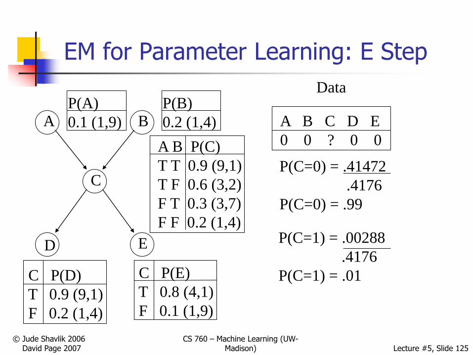
EM for Parameter Learning: E Step
C P(D)
T 0.9 (9,1)
F 0.2 (1,4)
A B
C
D E
P(A)
0.1 (1,9)
A B P(C)
T T 0.9 (9,1)
T F 0.6 (3,2)
F T 0.3 (3,7)
F F 0.2 (1,4)
P(B)
0.2 (1,4)
C P(E)
T 0.8 (4,1)
F 0.1 (1,9)
A B C D E
0 0 ? 0 0
Data
P(C=0) = .41472
.4176
P(C=0) = .99
P(C=1) = .00288
.4176
P(C=1) = .01
© Jude Shavlik 2006David Page 2007
CS 760 – Machine Learning (UW-Madison) Lecture #5, Slide 126
EM for Parameter Learning: E Step
C P(D)
T 0.9 (9,1)
F 0.2 (1,4)
A B
C
D E
P(A)
0.1 (1,9)
A B P(C)
T T 0.9 (9,1)
T F 0.6 (3,2)
F T 0.3 (3,7)
F F 0.2 (1,4)
P(B)
0.2 (1,4)
C P(E)
T 0.8 (4,1)
F 0.1 (1,9)
A B C D E
0 0 0 0
0 0 1 0
1 0 1 1
0 0 0 1
0 1 1 0
0 0 0 1
1 1 1 1
0 0 0 0
0 0 1 0
0 0 0 1
Data
0: 0.99
1: 0.01
0: 0.99
1: 0.01
0: 0.02
1: 0.98
0: 0.80
1: 0.20
0: 0.80
1: 0.20
0: 0.80
1: 0.20
0: 0.80
1: 0.20
0: 0.80
1: 0.20
0: 0.70
1: 0.30
0: 0.003
1: 0.997

© Jude Shavlik 2006David Page 2007
CS 760 – Machine Learning (UW-Madison) Lecture #5, Slide 127
EM for Parameter Learning: M Step
C P(D)
T 0.9 (9,1)
F 0.2 (1,4)
A B
C
D E
P(A)
0.1 (1,9)
A B P(C)
T T 0.9 (9,1)
T F 0.6 (3,2)
F T 0.3 (3,7)
F F 0.2 (1,4)
P(B)
0.2 (1,4)
C P(E)
T 0.8 (4,1)
F 0.1 (1,9)
A B C D E
0 0 0 0
0 0 1 0
1 0 1 1
0 0 0 1
0 1 1 0
0 0 0 1
1 1 1 1
0 0 0 0
0 0 1 0
0 0 0 1
Data
0: 0.99
1: 0.01
0: 0.99
1: 0.01
0: 0.02
1: 0.98
0: 0.80
1: 0.20
0: 0.80
1: 0.20
0: 0.80
1: 0.20
0: 0.80
1: 0.20
0: 0.80
1: 0.20
0: 0.70
1: 0.30
0: 0.003
1: 0.997
C = 0
4+
.99 +
.8 +
.8 +
.8 +
.99+
.8+
.8 +
=
9.98
© Jude Shavlik 2006David Page 2007
CS 760 – Machine Learning (UW-Madison) Lecture #5, Slide 128
EM for Parameter Learning: M Step
C P(D)
T 0.9 (9,1)
F 0.2 (1,4)
A B
C
D E
P(A)
0.1 (1,9)
A B P(C)
T T 0.9 (9,1)
T F 0.6 (3,2)
F T 0.3 (3,7)
F F 0.2 (1,4)
P(B)
0.2 (1,4)
C P(E)
T 0.8 (4,1)
F 0.1 (1,9)
A B C D E
0 0 0 0
0 0 1 0
1 0 1 1
0 0 0 1
0 1 1 0
0 0 0 1
1 1 1 1
0 0 0 0
0 0 1 0
0 0 0 1
Data
0: 0.99
1: 0.01
0: 0.99
1: 0.01
0: 0.02
1: 0.98
0: 0.80
1: 0.20
0: 0.80
1: 0.20
0: 0.80
1: 0.20
0: 0.80
1: 0.20
0: 0.80
1: 0.20
0: 0.70
1: 0.30
0: 0.003
1: 0.997
C = 1
1+
.01 +
.2 +
.2 +
.2 +
.01+
.2+
.2 +
=
2.02
C P(D)
T 0.9 (9,1)
F 0.2 (1,4)
A B
C
D E
P(A)
0.1 (1,9)
A B P(C)
T T 0.9 (9,1)
T F 0.6 (3,2)
F T 0.3 (3,7)
F F 0.2 (1,4)
P(B)
0.2 (1,4)
C P(E)
T 0.8 (4,1)
F 0.1 (1,9)
© Jude Shavlik 2006David Page 2007
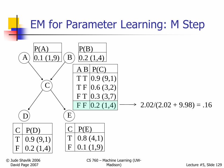
CS 760 – Machine Learning (UW-Madison) Lecture #5, Slide 129
EM for Parameter Learning: M Step
2.02/(2.02 + 9.98) = .16
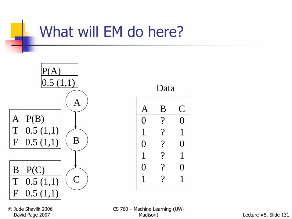
Problems with EM
Only local optimum
Deterministic: Uniform priors can cause issues
See next slide
Use randomness to overcome this problem
130
© Jude Shavlik 2006David Page 2007
CS 760 – Machine Learning (UW-Madison) Lecture #5, Slide 131
What will EM do here?
A
B
C
Data
A B C
0 ? 0
1 ? 1
0 ? 0
1 ? 1
0 ? 0
1 ? 1
P(A)
0.5 (1,1)
B P(C)
T 0.5 (1,1)
F 0.5 (1,1)
A P(B)
T 0.5 (1,1)
F 0.5 (1,1)

Outline
Probability overview
Naïve Bayes
Bayesian learning
Bayesian networks
Representation
Inference
Parameter learning
Structure learning
132
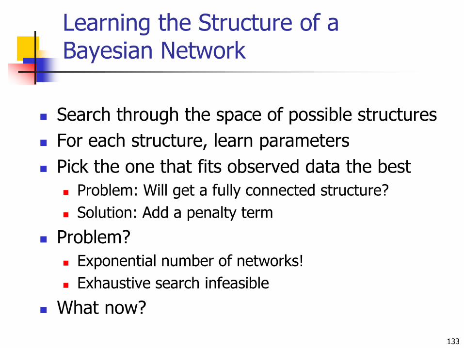
Learning the Structure of a Bayesian Network
Search through the space of possible structures
For each structure, learn parameters
Pick the one that fits observed data the best
Problem: Will get a fully connected structure?
Solution: Add a penalty term
Problem?
Exponential number of networks!
Exhaustive search infeasible
What now?
133
Structure Learning as Search
Local search
Start with some network structure
Try to make a change: Add, delete or reverse an edge
See if the new structure is better
What should the initial state be
Uniform prior over random networks?
Based on prior knowledge
Empty network?
How do we evaluate networks?134
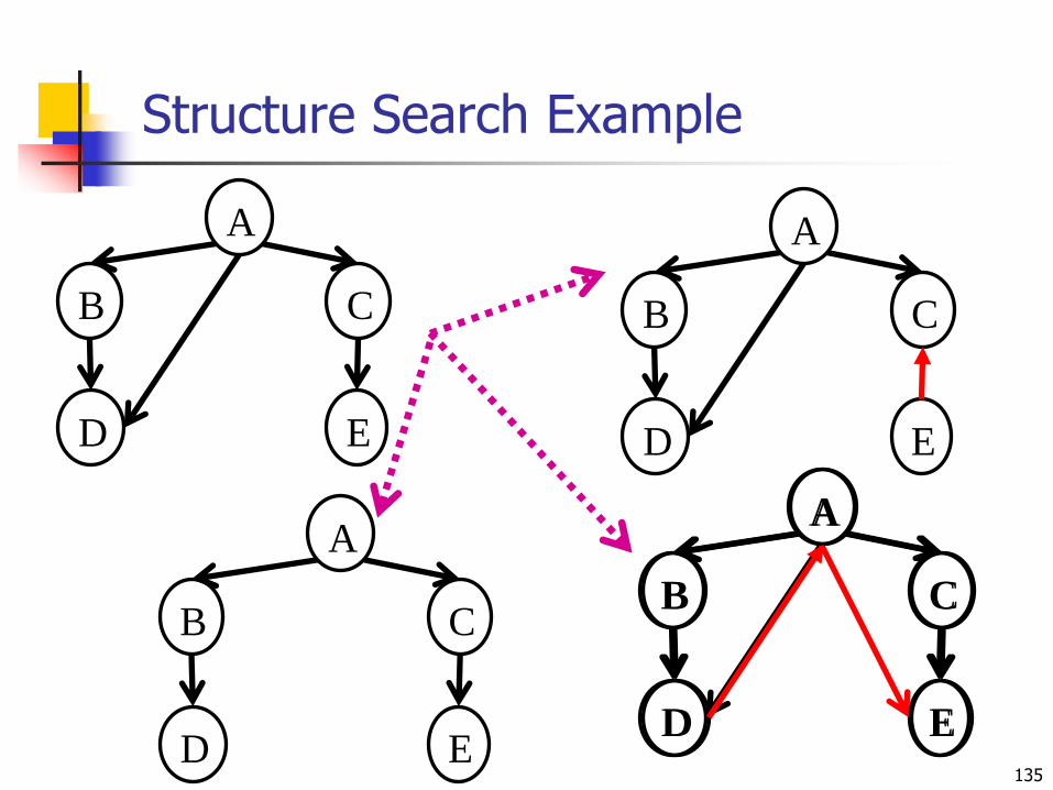
Structure Search Example
135
A
E
C
D
B
A
E
C
D
B
A
E
C
D
B
A
E
C
D
B
A
E
C
D
B
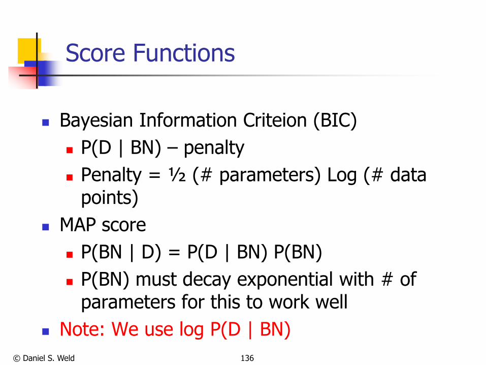
Score Functions
Bayesian Information Criteion (BIC)
P(D | BN) – penalty
Penalty = ½ (# parameters) Log (# data points)
MAP score
P(BN | D) = P(D | BN) P(BN)
P(BN) must decay exponential with # of parameters for this to work well
Note: We use log P(D | BN)
© Daniel S. Weld 136
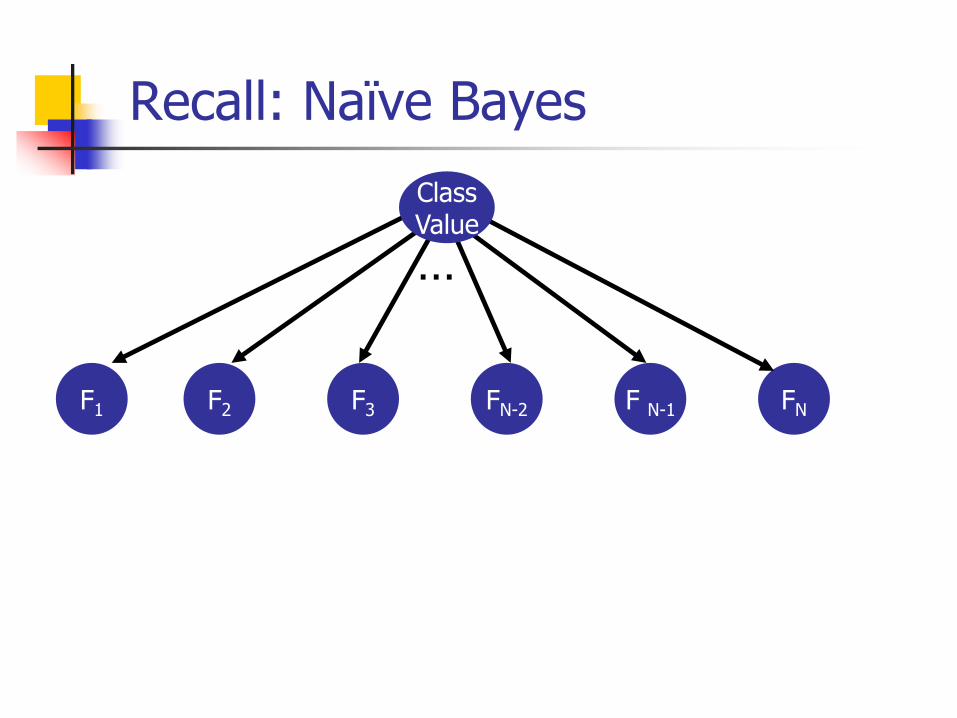
Recall: Naïve Bayes
F2 FN-2 F N-1 FNF1 F3
ClassValue
…

Tree Augmented Naïve Bayes (TAN) [Friedman,Geiger & Goldszmidt 1997]
F2 FN-2 F N-1 FNF1 F3
ClassValue
…
Models limited set of dependenciesGuaranteed to find best structureRuns in polynomial time

Tree-Augmented Naïve Bayes
Each feature has at most one parent in addition to the class attribute
For every pair of features, compute the conditional mutual informationIcm(x;y|c) = Σx,y,c P(x,y,c) log [p(x,y|c)/[p(x|c)*p(y|c)]]
Add arcs between all pairs of features, weighted by this value
Compute the maximum weight spanning tree, and direct arcs from the root
Compute parameters as already seen

Next Class
Proposition rule induction
First-order rule induction
Read Mitchell Chapter 10
140

Summary
Homework 2 is now available
Naïve Bayes: Reasonable, simple baseline
Different ways to incorporate prior beliefs
Bayesian networks are an efficient way to represent joint distributions
Representation
Inference
Learning
141

Questions?
142


