Nobel Lecture: Measuring the acceleration of the cosmic expansion using supernovae

Nobel Lecture: Measuring the acceleration of the cosmic expansion using

supernovae*

Saul Perlmutter

University of California at Berkeley and Lawrence Berkeley National Laboratory, Berkeley,California 94720, USA

(published 13 August 2012)

DOI: 10.1103/RevModPhys.84.1127

The ‘‘discovery of the acceleration of the expansion of the

Universe’’ does not flow trippingly off the tongue—which is

fitting, since the work that led to it was comparably long and

tortuous. In this Lecture, I would like to give you a feel for

some of the science issues we were facing over the ten years

leading up to the discovery. I will primarily use the graphics

from the original overhead projector transparencies we were

using in those years. Although they are not as beautiful as our

modern-day graphics, I hope they will help give some of the

texture of what was going on during that period.The question that motivated all this work is something you

can imagine that the very first humans might have asked when

they walked out of their caves at night and found themselves

looking up at the starry sky. Do we live in a universe that goes

on forever in space and will it last forever in time? I think it

almost defines what it means to be the very first humans—that

they could ask such questions.For most of human history, this sort of question was a truly

philosophical question. It was not until the 20th century that

we began to have a scientific version of this question. This is

partly because Einstein’s theory of general relativity gave us

some new conceptual tools that made it possible to think

about this topic in a more rigorous way. But it is also because

Edwin Hubble (1929) measured an expansion of the

Universe, which meant that we started to see in more concrete

terms what we could mean by the fate of the Universe.Hubble’s observations indicated that we do not live in a

universe that is standing still, but rather one in which all of the

distances between galaxies are growing with time. You can then

immediately start asking yourself whether it will continue to grow

with the same speed over time, or might it slow down because

gravity would attract all stuff to all other stuff in the Universe. In

fact, you might wonder if it could be slowing enough so that

someday it could come to a halt, and then collapse into a big

crunch—that could be the end of the Universe.This is a question about the future of the Universe that you

can address by looking into the past of the Universe, by

looking to see what was happening billions of years ago

and how much the Universe was slowing down back then.

If it was slowing enough, you could predict that it is slowing

enough to collapse in the future. This was understood, even

back in the 1930s, in the decade following Hubble’s discov-

ery, by astronomers like Walter Baade and Fritz Zwicky who

were studying supernovae. They saw that in principle, youcould use a very bright exploding star, a supernova, toperhaps answer this question. I will show you why that wouldbe possible.

You could take the brightness of a supernova as an indi-cator of how far away it is: the fainter it is, the farther away itis from us—and hence its light has taken more time to reachus. So with the fainter supernovae, you are looking farther andfarther back in time. You can also use the colors of thespectral features of a supernova: a supernova would lookblue if it were seen nearby, but when you see it very, veryfar away it looks red. How red it gets tells you how much theUniverse has stretched since the supernova exploded, becausewhile the light is traveling to us, its wavelength stretches bythe exact same proportion as the Universe stretches.

So this is a very direct way of plotting how much theUniverse has stretched as a function of time. In principle, ifyou observe enough supernovae and plot them on such agraph, you can see just how much the Universe has decel-erated in the past and make a prediction about how much itwill slow down in the future. Baade (1938) wrote about thispossible supernova measurement back in the 1930s. Theproblem was that the supernovae that they knew about atthat time were not quite good enough ‘‘standard candles’’;they were not all quite the same brightness. They varied bymore than a factor of 2 or 3 in brightness, so while it lookedlike a good idea, it was not really practical to do at that time.

That is essentially where the problem stood for about thenext 50 years [see Kowal (1968) for a benchmark along theway], until two things happened in the mid-1980s that got meand others interested in the problem: First, there was therealization that the supernovae could be subdivided intosubclassifications, and it was in the mid-1980s that the‘‘type Ia’’ subclassification was identified (Panagia, 1985;Uomoto and Kirshner, 1985; Wheeler and Levreault, 1985).It began to be clear that this one subclassification really was abetter standard candle than the others. For example, a histo-gram of supernova brightnesses in a paper by Nino Panagiashowed that supernovae found in spiral galaxies variedgreatly, while those found in elliptical galaxies had only asmall dispersion (see Fig. 1). The implication was that theellipticals might host a subclassification that was a betterstandard candle, and also that the spiral galaxies are knownto have dust that would add further dispersion. The possibilitythat we now had a good standard candle suggested that wenow might be ready to go back to the original idea of Baadeand Zwicky.

*The 2011 Nobel Prize for Physics was shared by Saul Perlmutter,

Adam G. Riess, and Brian P. Schmidt. These papers are the text of

the address given in conjunction with the award.

REVIEWS OF MODERN PHYSICS, VOLUME 84, JULY–SEPTEMBER 2012

0034-6861=2012=84(3)=1127(23) 1127 � 2012 Nobel Foundation, Published by The American Physical Society

http://dx.doi.org/10.1103/RevModPhys.84.1127

The other development of the mid-1980s was the introduc-tion into astronomy of the new sensors, the CCD detectors,which are like the detectors in the back of the digital camerasthat most people have today. These were just becomingavailable in the beginning of the 1980s, and I worked onone of the first astronomy projects to use CCD’s—as well asthe new computers that were just then becoming fast enoughto analyze the large amounts of data that came out of thesedetectors. This was a project led by my inspiring thesisadvisor, Richard Muller. It was doing a search for nearbysupernovae using a small robotic telescope and automaticdetection of the supernovae by the computers (see Fig. 2).I worked on the software that made it possible to subtract theimage of a galaxy from the image of a supernova plusthe galaxy, and thus find these supernovae (see Fig. 3).With the automatic searching technique we found 20 super-novae by the time the project stopped (Muller et al., 1992;see Fig. 4).

These two developments led Carl Pennypacker and myself,both of us researchers in Rich Muller’s group at that time in1987 (I had stayed on as a postdoc after just completing myPh.D.), to decide to try out the original idea of Baade andZwicky to measure the deceleration of the Universe’s expan-sion using supernovae. We began working on the project withRich’s support, and it looked very promising; however, wewere aware that it was not going to be easy. For a number ofreasons we knew there was a lot of work to be done to makethis possible. So when we proposed the project we did not getan immediately enthusiastic response from the referees andreviewers. But it is Carl’s nature to be absolutely undauntedand to be optimistic that we can do anything, and so we

carried on. There were the practical problems of trying to findthe more distant supernovae. There were some specifictechnical problems concerning how you would analyze thosevery faint, distant supernovae and compare them to nearbyexamples. There were issues about the standardness of thesupernovae themselves and their consistency over time thatneeded to be addressed. These were the specific details thatwe saw as the hurdles that had to be jumped over in order todo the project (see Fig. 5).

I will try to describe how we addressed these problems,because what is interesting about this particular measurementis that it is so simple to describe that it is possible to explainthe difficulties in some detail, and most people can thenunderstand what it would take to do this particular project.

First of all, there are the questions of can you find thesesupernovae at all, can you find them far enough away, can youfind enough of them, and can they be found early enough sothat they can brighten and then fade away and you can

FIG. 1. Histogram of supernova absolute magnitudes. From

Panagia, 1985.

FIG. 2. Saul Perlmutter and Richard Muller with a new telescope

the group was automating to replace the Leuschner Observatory

telescope (though it was later used for a different purpose at

another site).

FIG. 3. Example of digital image subtraction. From the CCD

image of a supernova and its host galaxy, we subtract an image

of the galaxy before the supernova appeared (or after it disap-

peared), leaving an image of just the supernova.

1128 Saul Perlmutter: Nobel Lecture: Measuring the acceleration of . . .

Rev. Mod. Phys., Vol. 84, No. 3, July–September 2012

measure the peak brightness? The peak brightness is what weknew was standard, so we could not use them if we foundthem weeks after they had already peaked. These were verydifficult problems, because if you had to choose a researchtool, you would never choose a supernova—it is a real pain inthe neck to do research with (see Fig. 6). They are rare: thetype Ia supernovae explode only a couple of times permillennium in a given galaxy. They are random: they donot tell you when they are going to explode. They brightenand fade away in time scales of weeks, so they do not stickaround so that you can study them. They are just veryinconvenient to do research with.

The difficulties were illustrated when we later saw theresults from another supernova project, which we learned

had started shortly before ours. Hans Nørgaard-Nielsen anda Danish team searched several years for very distant type Iasupernovae but found just one, several weeks after it hadalready passed its peak brightness (Nørgaard-Nielsen et al.,1989). So, while it was encouraging that such distant super-

novae existed, the critics of our project said that this did notlook like a very viable program. This was the first concern.

The approach that we took to this problem was to developthe capability to look at more than one galaxy at a time (sincelooking at one galaxy would have meant waiting the 500 yearsfor a type Ia supernova to explode), and even more than a

small cluster of galaxies at a time (as the Danish program haddone). We decided to build a wide-field camera that wouldallow us, with each exposure, to look at 10 to 20 times asmany galaxies as you would find even in a cluster of galaxies.

We had to develop an unusual optical system (see Fig. 7) thatwould bring light from a very big field of view onto a smallCCD detector. This novel instrument went onto the Anglo-Australian 4-m telescope; this meant that we were able to

work with a large enough telescope with a large enough fieldof view to be able to search for supernovae at great distancesin thousands of galaxies at a time.

FIG. 4. Before-and-after images of one of the supernovae discov-

ered in 1986 by our Berkeley Automated Supernova Search, led by

Professor Richard Muller.

FIG. 5 (color). Some of the issues that we recognized as hurdles to

be crossed in order to use supernovae to measure the deceleration of

the Universe’s expansion.

FIG. 6 (color). The characteristics of type Ia supernovae that

make them difficult to find and study over their peak brightness.

FIG. 7 (color). The novel F=1 wide-field CCD camera we devel-

oped for the Anglo-Australian 4-m telescope (AAT) to collect a

wide enough field to search for z > 0:3 type Ia supernovae in

hundreds of galaxies with each image.

Saul Perlmutter: Nobel Lecture: Measuring the acceleration of . . . 1129


With our wide-field camera on the Anglo-Australian tele-scope you obtain images like the one shown in Fig. 8, inwhich all the small specks of light are the distant galaxies inwhich we were searching for supernovae. You then take animage another time in the year (see Fig. 9) and subtract itfrom the first one. You are left with an image that shows justthe spot that got bright—and that is your supernova. Ofcourse we did this in software, so we had to go back to ourimage analysis software and develop that much further.Figure 10 shows what the computer subtraction looked like.Figure 11 shows some of the members of the group at thattime.

This method of finding supernovae seemed to work; how-ever the remaining problems were still haunting us, becauseeven if you could find the supernova you could not prove that

you had a supernova, since you would need to schedule thelargest telescopes in the world to obtain the identifyingspectrum. You would also need to schedule the largesttelescopes in the world to follow it as it brightens andfades away, to measure its brightness at peak. Of course, notelescope time assignment committee would give you thetime to schedule a telescope six months in advance for asupernova that may or may not appear on the proposedobserving date, say March 3rd.

As Mario Hamuy et al. (1993a) put it, in their discussionof the Calan/Tololo Supernova Search at much lower red-shifts, ‘‘Unfortunately, the appearance of a SN is not predict-able. As a consequence of this we cannot schedule the follow-up observations a priori, and we generally have to rely onsomeone else’s telescope time. This makes the execution ofthis project somewhat difficult.’’

FIG. 8. Image obtained November 1989 with our wide-field cam-

era on the Anglo-Australian 4-m telescope. The small specks of

light are the distant galaxies in which we were searching for

supernovae.

FIG. 9. The same field as in Fig. 8, but observed January 1990. It

is reversed in gray scale to indicate that it will be subtracted from

the first.

FIG. 10. Computer subtraction of Fig. 9 image from Fig. 8 image.

The spot remaining is what a supernova would look like.

FIG. 11. Members of the group in 1992 discuss images with many

distant galaxies obtained with a wide-field camera for the distant

supernova search. Left to right: Carl Pennypacker, Saul Perlmutter,

Heidi Marvin Newberg, Gerson Goldhaber, and Rich Muller.



So we had to figure out a way to make the whole operation

more systematic, and what we came up with was a new search

strategy that I developed to make this possible. Figure 12

shows the strategy on the time line of new moon to full moon

to new moon. I realized that if you collect all of your first

images just after new moon, wait 2 and 12 weeks or so, and

collect all of the second set of images just before the next new

moon (and then subtract all the second set from the first set),

you now have enough galaxies collected with a wide-field

imager to guarantee not just one supernova discovery, but

more than half a dozen supernova discoveries. Once you

reach this statistically significant sample size of supernovae,

then you can be sure that you always have some new super-

novae to observe by the second new moon. The other advan-

tage is that with this short time scale between the two sets of

images, you can guarantee that the supernovae will not have

enough time to reach maximum and then start fading away;

since they rise in a couple of weeks and fade in a few months,

this time scale ensures that you always catch them while they

are still brightening. You can then guarantee that right before

that second new moon, which is the time that you need to do

the spectroscopy, you will have new supernovae, they will be

on the rise, and there will be more than one. Now you can

schedule the follow-up spectroscopy and photometry on the

following nights.Once we demonstrated this, we were able to start applying

for telescope time at the best telescopes in the world for this

purpose, the telescopes in Chile, where the weather is good

enough that you can usually follow this whole time series

without getting hit by clouds and rain. The first time that we

tried this new ‘‘batch’’ observational strategy we called up the

International Astronomical Union telegram service, which

notifies astronomers around the world when a new supernovais discovered so it can be studied. They are very careful aboutwhat they allow in the telegram and I wanted to be sure theywould be able—and willing—to accept our results. I warnedthem that we would be sending them a half a dozen newsupernova discoveries two weeks from now. They laughed,because nobody had ever predicted a supernova discoverybefore, and certainly nobody ever found more than one at atime before, so it sounded a little unusual. In fact, we thensent out such telegrams semester after semester for thefollowing years, as this new observing technique worked,producing batches of supernovae.

So this did work and we had surmounted the problem ofmaking the supernova a systematic tool.

The next problem was that even if you found the super-novae there was the question of whether you could identifythe subtype, i.e., the type Ia’s. It was not clear that they wouldbe bright enough to obtain a reasonable spectrum. In fact thefirst spectra that we obtained looked mostly like a lot of noise.We realized, however, that we could take advantage of thefact that the spectral features of supernovae are very broad onthese wavelength scales, unlike the narrow spectral featuresof the underlying host galaxy and the noise. (This is becausethe supernova explosion spreads the spectral features out overa wide range of wavelengths, due to the Doppler shifts.)That meant that we could cut out all the sharp lines, andthen smooth the whole spectrum, in order to bring out the

FIG. 12 (color). The ‘‘batch’’ observational strategy that made it

possible to guarantee multiple new supernova discoveries at high

redshift, all on a prespecified date (in particular, just before a new

moon) and all while still brightening (Perlmutter et al., 1995a). This

in turn made it possible to propose many months in advance for

scheduled telescope time (in particular, during dark time) at the

largest telescopes to study the supernova over the peak of their light

curves with both photometry and spectroscopy.

FIG. 13. Spectrum of a high-redshift type Ia supernova. From

Lidman et al., 2005.

FIG. 14 (color). Same spectrum from Fig. 13, after removing very

narrow spectral features, and smoothing to bring out the broad

supernova features. The red curve shows the excellent match with a

spectrum of a low-redshift type Ia supernova, as it would appear

redshifted to z ¼ 0:55.



broad features that then did look like a supernova (seeFigs. 13 and 14).

Once we were able to show this, it became believable thatwe could identify the supernovae at these great distances. Italso helped that the larger telescopes came online just at thistime, for example, the Keck telescope that was being devel-oped just upstairs from me at Lawrence Berkeley Laboratorywhile I was a graduate student. At that time, I had no idea thatI would be using it, but just a few years later—as it was beingcommissioned—it was exactly the telescope that we neededto do this kind of work.

Another problem arises because the spectrum of a low-redshift supernova gets shifted to the redder wavelengthswhen you look at supernovae at greater distances—that iswhat we mean by ‘‘redshift.’’ Seen nearby, most of the light ofthe supernova is emitted in the blue wavelengths, so typicallyat low redshifts we study the supernova using the B-bandfilter (‘‘B’’ for ‘‘blue’’). But at high redshift the same blue

filter would be looking at the very faint UV tail of thespectrum (see Fig. 15). The question is how are you goingto compare a supernova seen in this faint tail of the spectrumwith a supernova seen at the peak of the spectrum? This kindof comparison is called a K correction, and whether itcould be done well enough to compare low- and high-redshiftsupernovae was far from clear. A paper by Bruno Leibundgut(1990) tried to show what the correction would have to be toaccount for the difference between the different parts of thetwo spectra. He did a very careful job, but the uncertainties inthe correction looked like they would present a significantproblem.

In 1992 we found the first high-redshift supernova that wewere able to follow throughout its entire light curve. It was ata redshift of z ¼ 0:45 (z stands for redshift). When we startedtrying to analyze it, we saw that the K correction everybodythought we would have to use was the wrong way to goabout it.

FIG. 15 (color). The standard ‘‘K correction’’ was intended to

capture the difference between the amount of light in a given filter

(here the B filter) seen at zero redshift and at high redshift, due to

the different parts of the spectrum that would be observed in that

filter. This was calculated for high-redshift supernovae by

Leibundgut (1990) and by Hamuy et al. (1993b).

FIG. 16 (color). The new ‘‘cross-filter K correction’’ developed by

Kim, Goobar, and Perlmutter (1996) worked by observing the high-

redshift supernova with a red filter, in this case the R-band filter, so

that the same part of the supernova spectrum is coming through this

filter at high redshift as comes through the B-band filter at low

redshift. This approach makes possible a much smaller uncertainty

for the K correction.



Instead of trying to find what part of the spectrum we were

looking at based on what the blue filter saw, what we really

had to do was look at the high-redshift supernova with a red

filter, the R-band filter. The same part of the spectrum that

comes through the R-band filter at high redshift is what comes

through the B-band filter at low redshift (see Fig. 16).

Alex Kim, Ariel Goobar, and I wrote a paper describing

this ‘‘cross-filter K-correction’’ approach, which made us

confident that we could control uncertainties that would

otherwise be introduced by the single-filter K correction

(Kim, Goobar, and Perlmutter, 1996; see also Nugent, Kim,

and Perlmutter, 2002).The next set of issues had to do with how standard were

these supernovae. Could you rely on them as a marker of

distances? The papers I mentioned earlier, for example,

Panagia (1985), were certainly suggestive of the possibility

that the type Ia supernovae could make a good standard.

Bruno Leibundgut (1988) and Gustav Tammann (Tammann

and Leibundgut, 1990) were really responsible for making the

community aware of how consistent the type Ia supernovae

were with each other, during the late 1980s and into the

1990s, so it is important to mention their names in this

context. It is also important to note David Branch’s group

(Miller and Branch, 1990; Branch and Tammann, 1992;

Branch and Miller, 1993) in Oklahoma, who were compiling

sets of published supernovae, and finding that they could

come up with ways to make them even more standard than

the earlier papers indicated.One good example of this was the paper by Vaughan et al.

(1995), which I worked on with the Oklahoma group, that

showed the improvement in the dispersion of type Ia super-

novae that was possible by simply rejecting the redder super-

novae (see Fig. 17). This would remove supernovae that were

dimmed by dust (making them appear redder), and also

peculiar supernovae that were intrinsically redder. This meant

that you could take the dispersion of brightness that you

observed from the 40% to 50% range that was seen in the

earlier data set down to something like a 30% dispersion, by

removing the redder supernovae. The Vaughn et al. paper

pointed out that this dispersion included measurement errors,

and since these were not very well-measured data sets the

measurement errors could, in fact, already account for most

of this 30% dispersion. So it was possible that the type Ia

supernovae were perfectly good standard candles but, given

the quality of data available, we just could not tell.In the early 1990s, the Calan-Tololo supernova search

joined in the game. This was a key moment for this field. I

particularly mention the names of Mario Hamuy, Jose Maza,

Mark Phillips, and Nick Suntzeff who were leaders in this

work, because they were responsible for setting the next

stage. The data set that they developed contained relatively

nearby supernovae that were just far enough out into the

Hubble flow so that you could measure the relative distances

very well (Hamuy et al., 1993a, 1996). Using the exact same

color cut from the Vaughn et al. paper, you could bring the

brightness dispersion down to about 18%, just by using this

better measured data set. Now this was good enough for the

cosmological measurement we wanted to make.There was another approach to this that Mark Phillips

proposed in the early 1990s: you could use the time scale

of the supernova event, e.g., how rapidly it decayed from its

peak brightness, to estimate what its brightness had been at

the peak of its light curve (see Fig. 18) (Phillips, 1993). Mark

saw this in the previously published supernova data, but even

more clearly in the new Calan-Tololo data. Adam Riess then

came up with a sophisticated statistical analysis of this, add-

ing and subtracting template light curve shapes (Riess, Press,

and Kirshner, 1995). Our group used a third method of

capturing this supernova time scale that I had developed:

simply stretching or compressing the time axis of the light

curve by a single ‘‘stretch factor’’ (Perlmutter et al., 1995a,

1997, 1999; see also Goldhaber et al., 1995, 2001).With this approach, you could take the range of beauti-

fully measured Calan-Tololo data that include brighter/

slower light curves as well as fainter/faster light curves,

and for each one measure the stretch factor that would be

needed to make them all match each other—and this stretch

factor would predict the brightness of each one. In fact, if

you ‘‘correct’’ each light curve by appropriately brightening

the faster ones and dimming the slower ones while stretch-

ing or compressing their time scales, you can standardize

all the light curves so that they all lie right on top of each

other (see Fig. 19).These techniques brought the field another step forward,

further improving the brightness dispersion from 18% down

to the 12%–15% range.With respect to the problem of dust dimming the super-

nova, I mentioned earlier that the color cut proposed by the

Oklahoma group in the Vaughan et al. paper not only re-

moved intrinsically redder supernovae, but also supernovae

that were dimmed (and reddened) by dust. Another way to

handle dust is to measure how red each supernova is, and then

correct the brightness for that amount of dust. [It was also

found that such a color correction can account for some color-

brightness relation intrinsic to the supernovae themselves,

FIG. 17 (color). One approach to improving the standardization of

the type Ia supernovae suggested by David Branch’s Oklahoma

group (Branch, Fisher, and Nugent, 1993; Vaughan et al., 1995)

was to remove all the redder supernovae (plotted here as red-filled

circles). This apparently removed both the dust-reddened super-

novae and many peculiar type Ia supernovae, thus greatly improving

the dispersion about the Hubble line.



since it appears to follow a very similar trend to dust’s (Tripp,

1998; Tripp and Branch, 1999)]. As I will discuss later, oncewe had proven the batch-discovery-and-follow-up technique

with that first batch of discoveries we were able to startgetting the telescope time to make better supernova measure-ments, including the good color measurements needed for

this purpose.An important element of this dust story is that apparently

most supernovae are not suffering much dimming by dust. Atthe time, you could already look at the range of relativebrightnesses and colors of nearby supernovae and see that

most supernovae were in a very narrow range—it would bespread more if dust were prevalent. And, of course, what you

really care about if you are comparing nearby and distantsupernovae is whether the range of supernova colors is thesame for both groups, indicating essentially the same dust

dimming. So we developed two approaches to this color study

of dust: you could compare the nearby and distant distribu-tions of supernova color, or you could correct each individual

supernova’s brightness using the color as an indication of howmuch correction is needed. (We used both of these approachesin the results that I will be discussing, and wewere thus able to

robustly account for the dust with our measurements.)There is also a third handle on dust that we began present-

ing at meetings, as an option for the future, if we could findeven more distant supernovae: At these much higher redshiftsit becomes possible to differentiate the dimming due to dust

from the cosmological effects. At great distances the super-nova events are so far back in time you would not expect dust

dimming to increase with distance the same way it does atcloser distances. The farther back you go, the more thedimming should be due to the cosmology and not to dust

FIG. 18 (color). Three alternative approaches to using the time scale of the supernova event (or the shape of the light curve) as an indicator

of how bright the supernova reached at peak. These methods followed Phillips (1993) recognition that the faster the supernova’s decline the

fainter its peak magnitude.



(see Fig. 20). In 1998 (Aldering et al., 1998), using theHubble Space telescope, we discovered, spectroscopicallyconfirmed, and measured the light curve of a supernova

with a redshift of 1.2—the first supernova ever found at aredshift above z ¼ 1. We nicknamed it Albinoni (see Fig. 20),

and it was the kind of supernova needed to perform thesetests. This approach was then taken to its conclusion by Adam

Riess and colleagues, in some beautiful Hubble SpaceTelescope (HST) work (Riess et al., 2004).

Finally, there is the concern that the supernovae are notguaranteed to act the same over billions of years. Since we are

looking so far back in time with these studies, the worrywould be that the supernovae back then might not be the same

as supernovae today. It would then be meaningless to com-pare the brightnesses if they were not identical. Our group

realized that there was a nice route to addressing this prob-lem: Just as the low-redshift supernova sample had beenseparated into those hosted by elliptical galaxies or spiral

galaxies, the same study could be performed for the high-redshift supernovae, and then the cosmology could be deter-

mined separately for the low- and high-redshift SNe found inelliptical galaxies and for those in spirals (see Fig. 21). These

different host-galaxy environments have very different his-

tories, so if the cosmology results from these different envi-

ronments agree we have a strong indication that the results are

not strongly distorted by the environmental histories chang-

ing the behavior of the supernovae.By mid-1994, we had answers in hand to the series of

concerns listed in Fig. 5 about using distant supernovae for

the cosmological measurement—but then we added one fur-

ther new concern (see Fig. 22). We began thinking about this

when we were analyzing the cosmological implications of

that very first high-redshift supernova that we found in 1992.

Of course, that one supernova by itself did not give you a very

definitive measurement, but it happened to come out with a

very low value for the slowing of the expansion of the

Universe, and hence the mass density of the Universe respon-

sible for this slowing. In fact, it was so low that we started to

think about a mathematical term called the ‘‘cosmological

constant’’ that Einstein had put into his equations describing

the Universe’s expansion. Einstein early on rejected this term,

once it was learned that the Universe was expanding. If it

were there, however, it would have the effect of fighting

against gravity’s slowing of the expansion. We realized that

our first supernova’s very low values for the slowing could be

due to some of this cosmological constant fighting against

gravity—and then how could you tell what you were seeing:

Is it less mass density, that is, less slowing due to gravity, or is

it perhaps more of the cosmological constant? The concern

was that we would not be able to tell these apart.Figure 23, from a paper that Ariel Goobar and I wrote

together, illustrates this problem. Say you have a supernova

with redshift z ¼ 0:5—which we did not yet, so this was still

hypothetical—and plot what combinations of mass density

and the density of the cosmological constant would be con-

sistent with its brightness. You get a steadily rising strip of

possible values. With just this plot, you would not know if the

true values describing our Universe were at the lower-left part

of this strip, with low mass density and low cosmological

constant density, or at the upper-right with high values for

both densities. What Ariel and I realized was that if you go

out to a larger range of redshifts, that is, if you study much

farther supernovae at redshifts as high as z ¼ 1 and beyond,

FIG. 19 (color). It is possible to ‘‘correct’’ each type Ia supernova

light curve by appropriately brightening the faster ones (low stretch

factor and dimming the slower ones (large stretch factor) while

stretching or compressing their time scales. The lower panel shows

the result of this, using a linear relation between the stretch of the

light curve time scale and its peak luminosity.

FIG. 20 (color). With the discovery (Aldering et al., 1998) of SN

1998eq (nicknamed ‘‘Albinoni’’), we showed that it was possible to

discover and spectroscopically confirm a type Ia supernova well

beyond redshift 1. We suggested that measurements at these very

high redshifts would make it possible to separate dust from cos-

mology in the dimming seen on the Hubble diagram.



then this plotted strip of allowed cosmological values starts torotate (see Fig. 24). Then the intersection of these strips fordifferent redshift supernovae allows us to separate out thesetwo effects—the mass density and the cosmological constantdensity—on the expansion history of the Universe.

Figure 25 shows the plot we used in the paper to show thatfor a given mass density you could distinguish between a zerocosmological constant—no cosmological constant at all—and a significant cosmological constant. Interestingly, thevalues we chose for this example of a significant cosmologi-cal constant turned out to be very close to the final answer wefound. Of course, we were expecting to find the zero-cosmo-logical-constant result shown. (We pointed out in the paperthat it would be easier to make the measurement if there were

a cosmological constant, because the error bars are smaller inthat region of this plot.)

Now we were in a position at the end of 1994 to use thenew on-the-rise and on-demand ‘‘batch’’ discovery strategyover and over again during each of the following semesters atthe telescopes. It became a production job: we wanted to turnout enough of these supernovae and make these delicate high-precision measurements in multiple colors so that we couldhave the strong statistical sample needed to measure howmuch the Universe is slowing down. We were by nowapplying to telescopes all around the world to do this. Wehad to use telescopes to find the supernovae (at the Cerro

FIG. 21. By performing the cosmology measurement with separate subgroups of supernovae found in different host-galaxy environments, it

is possible to test that the measurements are not strongly distorted by the different evolutionary histories at low and high redshift. We

proposed such tests in Perlmutter et al. (1995b, 1997, and 1999) and implemented them in several stages, leading to the HST-morphology-

based study shown here from our Sullivan et al. (2003) paper.

FIG. 22 (color). By 1994 there was new concern about the

supernova measurement—in addition to the four problems de-

scribed in Fig. 5.

FIG. 23 (color). Goobar and Perlmutter (1995) used this figure to

show that a measurement of a supernova at z ¼ 0:5 (hypothetical at

the time) would constrain the possible values of the mass density

and the cosmological constant density, but they could be traded

against each other along the strip of values shown here as a green

band.



Tololo 4-m telescope in Chile), to follow the supernovae with

spectroscopy (at the Keck 10-m telescope in Hawaii), to

follow the supernova with photometry (at the Isaac Newton

telescope in the Canary Islands and the WIYN telescope in

Tucson).So it was a pretty dramatic scene during the weeks that we

would conduct one of these supernova campaigns. One team

would be flying down to Chile and then returning to Chile

three weeks later for the ‘‘discovery images,’’ while another

team back in Berkeley would be pulling the data in near-real

time over the then-fledgling Internet to analyze the data.

Meanwhile teams would head out to Hawaii, the CanaryIslands, and Tucson, with email going back and forth updat-ing everything we knew about each supernova in our batch ofdiscoveries. By this time, the whole Supernova CosmologyProject (SCP) team was more than the three or four peoplethat we had at the beginning. Figure 26 shows much of theteam at that time. I want to emphasize what a capable,creative, and dedicated group of people this was, and itmade for a collaboration that was a great example ofteamwork.

Semester by semester, we started to build up this increas-ingly larger sample of type Ia supernovae, covering an in-creasing redshift range. In Fig. 27 the color coding shows thesupernova redshifts for each batch of supernova discoveriesfrom a given semester’s search and follow-up: first a half adozen, and then a dozen, and then another dozen. . . and by1997 we had enough supernovae in hand to get results thatwere statistically significant.

As we added the new batches of high-redshift supernovae

to the Hubble diagram, publishing the results at each step, the

history of the Universe’s expansion slowly began to be

apparent. The very first data (the red points around a redshift

of z ¼ 0:4 on the upper plot of Fig. 28) appeared to favor a

slowing universe with no cosmological constant, but with

only seven supernovae the uncertainties were large. (These

were the very first high-redshift supernovae we had studied.

After we had used them to show that the batch-discovery-and-

follow-up method worked, we were able to request and obtain

sufficient follow-up time on major telescopes to make more

comprehensive measurements of the following batches of

supernovae. So the next supernovae were all much better

measured.)In a Nature article that appeared 1 January 1998, we then

reported that even one very-well-measured supernova—it had

FIG. 24 (color). The strip of possible values rotates in the plane of

mass density vs cosmological constant density when we observe a

supernova at higher redshifts (the results for a then hypothetical

z ¼ 1 supernova are shown here with the blue band). The inter-

section of such measurements at different redshifts allows the two

densities to be distinguished. From Goobar and Perlmutter, 1995.

FIG. 25. In Goobar and Perlmutter (1995), we gave a range of sample cosmologies to show how supernovae at, e.g., z ¼ 0:5 and z ¼ 1,could distinguish mass density from cosmological constant density. The examples in the right panel turned out to be particularly prescient,

since they showed that in a universe with significant cosmological constant the smaller error bands make it easier to confirm the cosmological

constant’s existence.



Hubble Space telescope observations—at twice the redshift

(the red point at z ¼ 0:83 on the upper plot of Fig. 28) alreadybegan to tell a different story, pointing to a universe with a

cosmological constant! But the evidence really became

strong almost immediately afterward with 42 supernovae

(the red points on the lower plot of Fig. 28). Now there was

a clear bulk of the supernova data indicating a universe that is

dominated by a cosmological constant, not ordinary matter.Plotting the same data as an expansion history of the

Universe (see Fig. 29, upper plot), we see that it does not

match any of the entire range of possible slowing histories

shown (the curved lines on the figure). Apparently we do not

live in a universe that is currently slowing in its expansion,

but rather a universe with one of the more interesting histories

shown in the bottom panel of Fig. 29: Its expansion rate used

to be slowing, but has been speeding up for the last half of its

history and presumably could speed up forever.Apparently we have a universe that is dominated by some

new ingredient, some previously unknown ‘‘dark energy’’

that makes the Universe expand faster and faster. It is so

rare that you come across something that is not part of our

current physics model. This is one of the best outcomes that

you could ever get in a project like this. I feel very lucky to be

able to work on this at all, because here was a project where

any result you could discover would be exciting: We might

have found that the Universe was infinite, or that it was finite

and going to come to an end. Either of these results would

have been great. Instead we found an answer that was even

better than ‘‘great,’’ in that it was a surprise. This is not

something that you can even wish for in science.This outcome is a perfect example of how science can

so often be two headed. On the one hand, it was only possible

to discover what came as a surprise to all of us because our

field, physics, had already made such great progress in under-

standing the Universe. Less than a century ago we had no idea

that there was more to the Universe than our own Milky Way.

The immense size of the Universe, the fact that it is

expanding, the fact that it is populated with such things as

exploding stars—all this and more had to be discovered

before we could do the work that led us to contemplate an

unknown form of energy that accounts for more than two-

thirds of everything there is.It is amazing how much we figured out, but on the other

hand it is amazing how big a mystery has opened up as a

result, and how much we still have left to discover. One of the

real pleasures of doing science—which will continue to be

true, I believe, on any given day for the next few centuries—is

that we have so much knowledge to build upon, yet there is

still so much for us to discover.These two aspects of science remind us that science is a

method, not a finished product. We do not know where it will

lead or what new, seemingly magical powers it will give us in

the future. We never know whether what we find will turn out

to be useful, but we do know that in the past, whenever we

FIG. 26 (color). A collaboration meeting of the Supernova

Cosmology Project in the late 1990s. Top row: Greg Aldering,

Saul Perlmutter, and Isobel Hook. Second row: Sebastian Fabbro

and Alex Kim. Third row: Rob Knop and Pilar Ruiz-Lapuente.

Bottom row: Peter Nugent, Ariel Goobar, and Gerson Goldhaber.

(Not shown: Reynald Pain, who was taking the picture.)

FIG. 27 (color). Each semester (shown in different colors) be-

tween 1994 and 1998 we employed the ‘‘batch search-and-

followup’’ method to add another set of type Ia supernovae. The

distance (redshift) range increased, and we began to use the Hubble

Space telescope to follow the SNe to obtain the most precise

measurements.



made a major step forward in our understanding of how theworld works, we have ultimately been able to solve moreproblems, including very practical problems. I think that isthe only way we can proceed as basic scientists: we try to seewhat we can understand, and we hope it opens more possi-bilities for what we can do in the world.

So far, you may have the impression of this science being avery cut-and-dried activity: we identify each problem, andsolve it, and then see the results. But the actual experience ofthis work is completely different: it is a nonstop whirlwind ofactivity and people. Unfortunately there are almost no photo-graphs of this 10 yr project to show this.

But a few years ago I tried to convey this with thefollowing very fast, impressionistic, verbal sketch of scenesfrom the decade leading up to the discoveries. (I will

supplement this with the few photos that we do have; seeFigs. 29–82.)

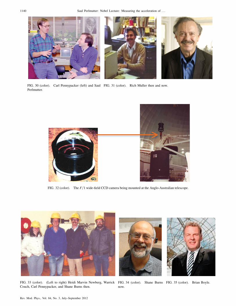
It begins with brainstorming at Berkeley with CarlPennypacker (in 1987) as we first batted around hardwareand software plans for a new high-redshift SN project in RichMuller’s group, which Rich soon embraced—and then theconsequence: the mountaintop observatory cafeteria atCoonabarabran as Carl, graduate student Heidi Newberg,former-graduate student Shane Burns, and I got to knowour pioneering Australia-based colleagues, Warrick Couchand Brian Boyle installing and then using our weird crystalball of a wide-field corrector and camera at the AAT 4-mtelescope—which led to our first high-redshift (but uncon-firmed) SN.

Back at Berkeley, I have an image of Gerson Goldhaberoverlaying transparencies with negative and positive imagesof fields full of galaxies—image analysis for the days whenthe computers were down!

FIG. 28 (color). As the SCP added the new batches of high-

redshift supernovae to the Hubble diagram the history of the

Universe’s expansion slowly began to be apparent (Perlmutter

et al., 1998). The very first data (the red points around a redshift

of z ¼ 0:4 on the upper plot) appeared to favor a slowing universe

with no cosmological constant, but with only 7 supernovae the

uncertainties were large. Even one very-well-measured supernova—

it had Hubble Space telescope observations—at twice the redshift

(the red point at z ¼ 0:83 on the upper plot) already began to tell a

different story. But the evidence really became strong with 42

supernovae (the red points on the lower plot). Now there was a

clear bulk of the supernova data indicating a universe that is

dominated by a cosmological constant, not ordinary matter. Its

expansion is apparently speeding up.

FIG. 29 (color). Our supernova data clearly did not fit with any of

the decelerating options shown in the upper panel. To fit the data, we

now had to add curves that are currently accelerating, as shown in

the blue region of the lower panel. The best fit curve was decelerat-

ing for about the first 7� 109 years, and then accelerating for the

most recent approximately 7� 109 years. This was the surprising

result the supernovae were showing us. Adapted from Perlmutter,

2003.



FIG. 30 (color). Carl Pennypacker (left) and Saul

Perlmutter.

FIG. 31 (color). Rich Muller then and now.

FIG. 32 (color). The F=1wide-field CCD camera being mounted at the Anglo-Australian telescope.

FIG. 33 (color). (Left to right) Heidi Marvin Newberg, Warrick

Couch, Carl Pennypacker, and Shane Burns then.

FIG. 34 (color). Shane Burns

now.

FIG. 35 (color). Brian Boyle.



FIG. 37 (color). Heidi Marvin Newberg.FIG. 36 (color). Warrick Couch then and now.

FIG. 38 (color). The group’s first (unconfirmed) high-redshift supernova, observed at the Anglo-

Australian telescope.

FIG. 39 (color). Gerson Goldhaber.



FIG. 40. Transparencies showing successive images of distant galaxies with computer subtraction to isolate possible supernova.

FIG. 41 (color). Anglo-Australian telescope in Coonabarabran,

Australia.

FIG. 42 (color). Isaac Newton telescope on La Palma in the

Canary Islands.

FIG. 44 (color). One of the preliminary

graphs showing the brightening and fading light

of the group’s first official high-redshift super-

nova, SN 1992bi. The plot is on a transparency

that is overlaid with another transparency show-

ing the expected light curve, based on nearby

type Ia supernovae.

FIG. 43 (color). Richard McMahon then and now.



I should pause here to say that we are very sad that Gersonis not here today—he died just over a year ago. He was awarm heart—and sharp eyes—of our team, and the host of thecollaboration parties, and he should have been here to cele-brate with us. We miss him.

In Australia, we had rain, rain, rain, and more clouds—andthen the sunny relief of beautiful La Palma where our newCambridge colleagues, Richard McMahon (working withMike Irwin) studied the most distant quasars. Long nightsdebugging a new instrument for La Palma, and tense phonecalls to the Isaac Newton telescope while the data were sentto Berkeley for analysis—and then our first ‘‘official’’high-redshift supernova—and a crucial La Palma spectrumfrom the Hirschel telescope as Richard Ellis has by nowjoined the team (after being one of those Danish grouppioneers).

By this time the Europeans had arrived full force atBerkeley: Ariel Goobar from Stockholm kicked it off, devel-oping new analyses with our then-grad student Alex Kim,brainstorming with me about the cosmological measure-ments. A glimpse of Reynald Pain from Paris assessing thedamage (and successes) at the end of a complex telescoperun—the first of the so-called ‘‘batch discoveries.’’ Thisepoch ends in my mind with a celebratory party at GersonGoldhaber’s in the Berkeley hills, where we have a bottle ofchampagne for each of the half dozen SNe discovered in abatch.

The sociology changes a little as we move to mass pro-duction, with new outposts at telescopes around the world,typically manned by a lone team member tenuously con-nected by a stream of email, phone, and fax. Pilar Ruiz-

FIG. 46 (color). Richard Ellis then and now.FIG. 45. Spectrum, obtained at the William Herschel tele-

scope on La Palma, of the galaxy that hosted SN 1992bi, the

group’s first official high-redshift supernova.

FIG. 47 (color). Ariel Goobar (left)

and Carl Pennypacker in 1998.

FIG. 48 (color). Ariel Goobar now. FIG. 49 (color). Alex Kim.



Lapuente and Nic Walton are at La Palma, Chris Lidman isthe voice at the VLT in Chile, and Brad Schaefer is at KittPeak. Larger expeditionary forces head to Cerra Tololo inChile where all the SN discoveries now are generated(I picture Don Groom and Susana Deustua on one suchtrip), immediately followed by another team of us rushingwith the new list of likely SNe to the oxygen poor mountain-

top of the then-new Keck telescope. I have a memory videoclip of Alex Filippenko—then on our team, his student TomMatheson, and our new Cambridge Ph.D. Isobel Hook and Icrowding round the computer screen as SN after SN proveditself. And at the control center in Berkeley the graduatestudents working around the clock: I picture Matthew Kim

FIG. 51 (color). An IAU circular reporting the re-

sults of a ‘‘batch’’ SN discovery observing run.

FIG. 50 (color). Reynald Pain.

FIG. 52 (color). Pilar Ruiz-Lapuente then

and now.FIG. 54 (color). Chris Lidman then and now.FIG. 53 (color). Telescopes around the

world.

FIG. 55 (color). Brad

Schaefer.

FIG. 56 (color). Don

Groom.

FIG. 57 (color). Susana

Deustua.

FIG. 58 (color). Alex

Filippenko.

FIG. 59 (color). Tom

Matheson.



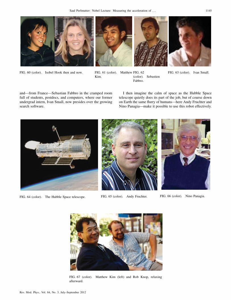
and—from France—Sebastian Fabbro in the cramped roomfull of students, postdocs, and computers, where our formerundergrad intern, Ivan Small, now presides over the growingsearch software.

I then imagine the calm of space as the Hubble Spacetelescope quietly does its part of the job, but of course downon Earth the same flurry of humans—here Andy Fruchter andNino Panagia—make it possible to use this robot effectively.

FIG. 60 (color). Isobel Hook then and now. FIG. 61 (color). Matthew

Kim.

FIG. 62

(color). Sebastien

Fabbro.

FIG. 63 (color). Ivan Small.

FIG. 64 (color). The Hubble Space telescope. FIG. 65 (color). Andy Fruchter. FIG. 66 (color). Nino Panagia.

FIG. 67 (color). Matthew Kim (left) and Rob Knop, relaxing

afterward.



The last act begins with a view of the end-of-nightcleanup after the next collaboration party, but this timethere are entire cases of bottles of champagne left un-drunk—we are lightweights—all labeled with the names ofthe now scores of new SNe to be analyzed. A fresh reliefteam of scientists is now on the field at Berkeley: RobKnop, who thinks, types—and programs—faster than Italk, Peter Nugent, juggling SN theory and practice, andGreg Aldering pulling together all the strains of theanalysis . . .and the search.

A final push of analyses has all of our Berkeley-based pre-graduate-school interns working nights and weekends (par-allel computing at its finest): first Julia Lee, and then PatriciaCastro, Nelson Nunes, and Robert Quimby—all of whomcontinued careers in the field.

And we all fall gasping in a metaphorical heap with thesurprising discovery about the Universe that you just heardabout . . .. And that is just our science team!

I think it is pretty clear from all this that the popular imageof the lone scientist in a lab looks nothing like our experience:science is—at least for us—an extremely social activity. Thisparticular work was the product of an amazing community ofscientists. Between our two teams, in fact, we include a largefraction, but not all of that community of scientists studyingsupernova—and just representing the rest of this supernovacommunity I show here several of the key players that Imentioned in the talk, with whom it was an honor and apleasure to work on this.

None of this whirlwind of human choreography happenswithout the constant support of our families and friends, ourteachers and mentors—and our staff at the universities, labo-

FIG. 68 (color). Rob Knop. FIG. 69 (color). Peter Nugent then and now.

FIG. 70 (color). Greg Aldering then and now.



FIG. 71 (color). Julia Lee then and now.

FIG. 72 (color). Robert Quimby then and now.

FIG. 73 (color). Nelson Nunes and

Patricia Castro then.

FIG. 74 (color). Nelson Nunes now. FIG. 75 (color). Patricia Castro

now.

FIG. 76 (color). The Supernova Cosmology Project team in 2007.



ratories, and observatories—and also, in many cases, thereally courageous administrators and funders who took riskson things when it was not obvious they were going to work.They are represented today by the family and friends who arehere and we all thank you for helping—and putting up with—all this.

But the work is not done! We look forward to joining inwith the next tag teams of scientists as we delve into themystery that we are currently calling dark energy.

And, finally, we are grateful for the Nobel Prize commit-tees and foundation, who have found a way to encourage thishuman activity of science.

Thank you.

REFERENCES

Aldering, G., et al., 1998, IAUC 7046, 1A [http://www.cbat

.eps.harvard.edu/iauc/07000/07046.html].

FIG. 77 (color). The High-Z Supernova Search team in 2007.

FIG. 80 (color). Craig Wheeler. FIG. 81. Gustav Tammann. FIG. 82 (color). David Branch.

FIG. 79 (color). Mario Hamuy.FIG. 78 (color). Jose Maza.



http://www.cbat.eps.harvard.edu/iauc/07000/07046.html

http://www.cbat.eps.harvard.edu/iauc/07000/07046.html

Baade, W., 1938, Astrophys. J. 88, 285.

Branch, D., A. Fisher, and P. Nugent, 1993, Astron. J. 106, 2383.

Branch, D., and D. Miller, 1993, Astrophys. J. 405, L5.

Branch, D., and G. Tammann, 1992, Annu. Rev. Astron. Astrophys.

30, 359.

Goldhaber, G., et al., 1995, in ‘‘Four Papers by the ’Supernova

Cosmology Project,’’’ edited by S. Perlmutter, Lawrence Berkeley

Laboratory Report No. LBL-38400, also in Thermonuclear

Supernovae, edited by P. Ruiz-Lapuente, R. Canal, and J. Isern,

NATO ASI Series C, Vol. 486 (Kluwer, Dordrecht, 1997).

Goldhaber, G., et al., 2001, Astrophys. J. 558, 359.

Goobar, A., and S. Perlmutter, 1995, Astrophys. J. 450, 14.

Hamuy, M., et al., 1993a, Astron. J. 106, 2392.

Hamuy, M., et al., 1993b, Publ. Astron. Soc. Pac. 105, 787.

Hamuy, M., M.M. Phillips, N. B. Suntzeff, R. A. Schommer, J.

Maza, and R. Aviles, 1996, Astron. J. 112, 2398.

Hubble, E., 1929, Proc. Natl. Acad. Sci. U.S.A. 15, 168.

Kim, A., A. Goobar, and S. Perlmutter, 1996, Publ. Astron. Soc.

Pac. 108, 190.

Kowal, C. T., 1968, Astron. J. 73, 1021.

Lidman, C., et al., 2005, Astron. Astrophys. 430, 843.

Liebundgut, B., 1988, Ph.D. thesis (University of Basel).

Leibundgut, B., 1990, Astron. Astrophys. 229, 1.

Miller, D., and D. Branch, 1990, Astron. J. 100, 530.

Muller, R., H. .J.M. Newberg, C. R. Pennypacker, S. Perlmutter,

T. P. Sasseen, and C.K. Smith, 1992, Astrophys. J. 384, L9.

Nørgaard-Nielson, H. U., L. Hansen, H. E. Jørgensen, A. A.

Salamanca, R. S. Ellis, and W. J. Couch, 1989, Nature (London)

339, 523.

Nugent, P., A. Kim, and S. Perlmutter, 2002, Publ. Astron. Soc. Pac.

114, 803.

Panagia, N., 1985, Lecture Notes in Physics (Springer, Berlin/

Heidelberg), Vol. 224, p. 14.

Perlmutter, S., 2003, Phys. Today 56, No. 4, 53.

Perlmutter, S., et al., 1995a, in ‘‘Four Papers by the ‘Supernova

Cosmology Project,’’’ edited by S. Perlmutter, Lawrence Berkeley

Laboratory Report No. LBL-38400, also in Thermonuclear

Supernovae, edited by P. Ruiz-Lapuente, R. Canal, and J. Isern,

NATO ASI Series C, Vol. 486 (Kluwer, Dordrecht, 1997).

Perlmutter, S., et al., 1995b, Astrophys. J. 440, L41.

Perlmutter, S., et al., 1997, Astrophys. J. 483, 565.

Perlmutter, S., et al., 1998, Nature (London) 391, 51.

Perlmutter, S., et al., 1999, Astrophys. J. 517, 565.

Phillips, M., 1993, Astrophys. J. 413, L105.

Riess, A., W. Press, and R. Kirshner, 1995, Astrophys. J. 438, L17.

Riess, A., et al., 2004, Astrophys. J. 607, 665.

Sullivan, M., et al., 2003, Mon. Not. R. Astron. Soc. 340, 1057.

Tammann, G. A., and B. Leibundgut, 1990, Astron. Astrophys.

236, 9.

Tripp, R., 1998, Astron. Astrophys. 331, 815 [http://adsabs.harvard

.edu/abs/1998A%26A...331..815T].

Tripp, R., and D. Branch, 1999, Astrophys. J. 525, 209.

Uomoto, A., and R. P. Kirshner, 1985, Astron. Astrophys.

149, L7.

Vaughan, T., D. Branch, D. Miller, and S. Perlmutter, 1995,

Astrophys. J. 439, 558.

Wheeler, J. C., and R. Levreault, 1985, Astrophys. J. 294,

L17.



http://dx.doi.org/10.1086/143983

http://dx.doi.org/10.1086/116810

http://dx.doi.org/10.1086/186752

http://dx.doi.org/10.1146/annurev.aa.30.090192.002043

http://dx.doi.org/10.1146/annurev.aa.30.090192.002043

http://dx.doi.org/10.1086/322460

http://dx.doi.org/10.1086/176113

http://dx.doi.org/10.1086/116811

http://dx.doi.org/10.1086/118191

http://dx.doi.org/10.1073/pnas.15.3.168

http://dx.doi.org/10.1086/110763

http://dx.doi.org/10.1051/0004-6361:20041504

http://dx.doi.org/10.1086/115534

http://dx.doi.org/10.1086/186251

http://dx.doi.org/10.1038/339523a0

http://dx.doi.org/10.1038/339523a0

http://dx.doi.org/10.1086/341707

http://dx.doi.org/10.1086/341707

http://dx.doi.org/10.1063/1.1580050

http://dx.doi.org/10.1086/187756

http://dx.doi.org/10.1086/304265

http://dx.doi.org/10.1038/34124

http://dx.doi.org/10.1086/307221

http://dx.doi.org/10.1086/186970

http://dx.doi.org/10.1086/187704

http://dx.doi.org/10.1086/383612

http://dx.doi.org/10.1046/j.1365-8711.2003.06312.x

http://adsabs.harvard.edu/abs/1998A%26A...331..815T

http://adsabs.harvard.edu/abs/1998A%26A...331..815T

http://dx.doi.org/10.1086/307883

http://dx.doi.org/10.1086/175196

http://dx.doi.org/10.1086/184500

http://dx.doi.org/10.1086/184500

Date post:	09-Dec-2016
Category:	Documents
Upload:	saul
View:	213 times
Download:	0 times

Nobel Lecture: Measuring the acceleration of the cosmic expansion using supernovae

Documents