Noise mechanisms in laser diodes

IEEE TRANSADIONS ON ELECTRON DEVICES, VOL. 41, NO. I I , NOVEMBER 1994 2139

Noise Mechanisms in Laser Diodes B. Olle Nilsson

Invited Paper

Abstruct- Noise in diode laser applications. Basics of diode lasers. Differences and similarities between optical and electronic devices. Dynamics and fundamental noise mechanisms in laser diodes; special difficulties encountered; present level of understanding. Intensity noise and frequency noise. Fundamental limits. Why can a laser diode generate an optical beam with sub-Poissonian photon statistics? Noise in traveling wave laser diode amplifiers. Mode partition noise, transients and external reflections, jitter. Optical and electrical feedback. Future developments.

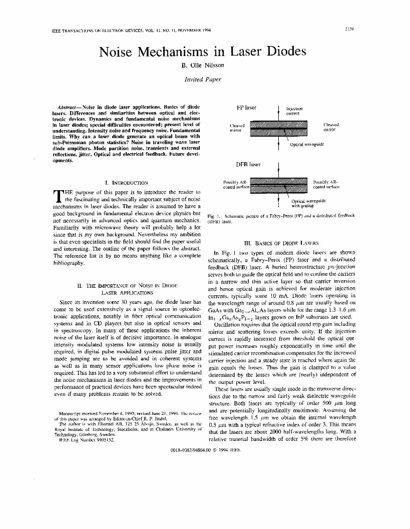
Injection current t FP laser

('lea\ ed Cleated mirror mirror

I \ 1 ' Optical waveguide

I DFB laser

I. INTRODUCTION

HE purpose of this paper is to introduce the reader to T the fascinating and technically important subject of noise mechanisms in laser diodes. The reader is assumed to have a good background in fundamental electron device physics but not necessarily in advanced optics and quantum mechanics. Familiarity with microwave theory will probably help a lot since that is my own background. Nevertheless my ambition is that even specialists in the field should find the paper useful and interesting. The outline of the paper follows the abstract. The reference list is by no means anything like a complete bibliography.

11. THE IMPORTANCE OF NOISE IN DIODE LASER APPLICATIONS

Since its invention some 30 years ago, the diode laser has come to be used extensively as a signal source in optoelectronic applications, notably in fiber optical communication systems and in CD players but also in optical sensors and in spectroscopy. In many of these applications the inherent noise of the laser itself is of decisive importance. In analogue intensity modulated systems low intensity noise is usually required, in digital pulse modulated systems pulse jitter and mode jumping are to be avoided and in coherent systems as well as in many sensor applications low phase noise is required. This has led to a very substantial effort to understand the noise mechanisms in laser diodes and the improvements in performance of practical devices have been spectacular indeed even if many problems remain to be solved.

Manuscript received November 4, 1993; revised June 21. 1994. The review of this paper was arranged by Editor-in-Chief,R. P. Jindal.

The author is with Ellemtel AB, 125 25 Alvsjo, Sweden. as well as the Royal Institute of Technology, Stockholm, and at Chalmers University of Technology, Goteborg, Sweden.

IEEE Log Number 9405152.

1 ' Optical waveguide with grating

Fig. I . (DFB) laser.

Schematic picture of a Fabry-Perot (FP) and a distributed feedback

111. BASICS OF DIODE LASERS

In Fig. 1 two types of modem diode lasers are shown schematically, a Fabry-Perot (FP) laser and a distributed feedback (DFB) laser. A buried heterostructure pn-junction serves both to guide the optical field and to confine the carriers in a narrow and thin active layer so that carrier inversion and hence optical gain is achieved for moderate injection currents, typically some 10 mA. Diode lasers operating in the wavelength range of around 0.8 pm are usually based on GaAs with Gal-,Al,As layers while for the range 1.3-1.6 pm In~-,Ga,As,P1-, layers grown on InP substrates are used.

Oscillation requires that the optical round trip gain including mirror and scattering losses exceeds unity. If the injection current is rapidly increased from threshold the optical output power increases roughly exponentially in time until the stimulated carrier recombination compensates for the increased carrier injection and a steady state is reached where again the gain equals the losses. Thus the gain is clamped to a value determined by the losses which are (nearly) independent of the output power level.

These lasers are usually single mode in the transverse direc- tions due to the narrow and fairly weak dielectric waveguide structure. Both lasers are typically of order 500 pm long and are potentially longitudinally multimode. Assuming the free wavelength 1.5 pm we obtain the intemal wavelength 0.5 pm with a typical refractive index of order 3. This means that the lasers are about 2000 half-wavelengths long. With a relative material bandwidth of order 5 % there are therefore

0018-9383/94$04.00 0 1994 IEEE

2140

about 100 different modes that may potentially oscillate. In stationary operation a Fp laser may run single mode with fairly good side-mode suppression but as soon as it is modulated it turns multimode. As a remedy of this behavior the DFB laser was developed [l]. Here the necessary optical feedback is not obtained by (wavelength independent) cleaved mirror reflections but by a wavelength selective Bragg grating. There are several types of such lasers which, if carefully designed, show a good single mode behavior even under fairly strong modulation [ 2 ] . By partitioning the electrode in several separately fed sections one can also achieve a certain degree of electric wavelength tunability (several nanometers) [3]. There are many conditions to fulfil in order to obtain such good results, however. If the end facets are not anti-reflection coated the position of the facets relative to the grating corrugation is very important. Since that is difficult to control this results in a low yield.

Other problems arise because of the inhomogeneous optical intensity distribution leading to a power dependent carrier density and gain distribution along the laser. Such so called spatial hole burning can easily lead to mode hopping and irregularities in the output power versus injection current characteristics [4]. This explains why there is still a lot of research devoted to improve DFB lasers.

We have, in fact, just illustrated one of the differences between lasers and electronic devices like transistor oscillators namely that the physical size of a laser normally is much larger than the wavelength. Therefore the maximum output power of a laser is basically independent of the wavelength as determined by the physical area of the device in contrast to the usual l/fz behavior of electronic devices. On the other hand serious problems with mode control and, sometimes noise induced, instabilities may arise as touched upon above.

Another more fundamental difference is that the noise in a diode laser is of quantum rather than thermal origin. Since noise is the central theme in this paper we will consider the meaning of this statement in some depth.

We will first state a few relations without derivation. From the theory of thermal noise we have the well known expression for the available noise power Pn from a resistive load of temperature T as measured within a bandwidth B:

P, = kTB (1)

where k = 1.38 . In the optical domain noise properties are dominated by

quantum fluctuations and (1) is no longer valid. Within certain limits to be discussed below, however, one may replace (1) with [5]

[WsK] is Boltzmann’s constant.

hu 2

P --B. n -

Thus kT has been replaced by hu/2, where h = 6.625.10-34 [Ws’] is Planck’s constant and U is the optical frequency. At room temperature, 300 K, the two expressions give the same result for U = 2kT/h = 1.25 . 1013 Hz corresponding to a wavelength of 24 pm. For wavelengths below about 2 pm we may therefore use (2) without any corrections for noise of thermal origin. In an optical system (1) and (2) describe

IEEE TRANSACTIONS ON ELECTRON DEVICES, VOL. 41, NO. 11, NOVEMBER 1994

the fluctuations originating from a matched termination in thermodynamical equilibrium into a single propagating mode just as in a microwave system.

We now add a “classical” noise free signal and denote its complex amplitude by A, normalized such that AA* is the power in the wave. Together with the so-called zero point fluctuations determined by (2) such a wave forms what quantum mechanically is called a coherent state [6] which is a minimum uncertainty state, i.e., in the sense that its fluctuations are the smallest allowed by Heisenberg’s uncertainty relation. Denoting the zero point fluctuations by b with single sided power spectral density S b = hu/2 according to (2), the total amplitude is A + b. The instantaneous power, P, is then given by ( A + b)(A + b)* so that

P = AA* + 2Re{Ab*} + bb* = Po + AP

where it is understood that the power bb* associated with the zero point fluctuations alone is not detected by a photo detector. This simple procedure yields the correct noise spectral density of the photo detector output but fails to give the correct photon statistics at very small photon numbers. The first term is the average power and the second is a fluctuating power of zero mean and of single sided power spectral density

Sap = 4AA*Sb = 2h~Po

since frequency components in b both below and above the signal frequency contribute and since sb = hu/2. Noting that the photon energy is hu we have arrived at the ordinary shot noise formula. A full quantum mechanical treatment indeed verifies that the ideal photo detection of a coherent state is a Poisson process. It has been a widespread misconception, however, that the shot noise is created in the detection process itself; it is now recognized that it is an inherent property of an electromagnetic field in a coherent state itself. We will come back to this question later.

The interpretation of (2) is straightforward in the case of a passive resistive load and expresses the fact that there is an inherent uncertainty in the electromagnetic field corresponding to a quantum mechanical ground state energy hu/2 related to Heisenberg’s uncertainty principle. In an active device like a laser, however, one has to consider the noise not only from the passive load but also from the active gain medium itself and the fact that both these noise contributions may be amplified due to the presence of gain. Fortunately it turns out from the quantum theory of electromagnetic fields that in a sense (2) is valid also for an active load consisting of a fully inverted population of carriers (no camers at the lower energy level). However, since the concept of available power from an active load is not easily defined we will rephrase (2) in terms of the average squared noise current from a conductance, G:

hu 2

( i2) = 4-GB (3)

which gives the available noise power according to (2). This holds also for active loads, i.e., for negative values

of G provided that the absolute value of G is used. In a realistic model of a diode laser one can represent each small region within which the optical field can be regarded

NILSSON: NOISE MECHANISMS IN LASER DIODES 2141

as spatially constant by a conductance in parallel with a susceptance [7 ] . Physically these currents are due to the oscillating dipoles of the carriers in the active volume and to other phenomena like free carrier absorption. In a lumped model of a diode laser, neglecting the spatial variation, we may represent optical loss and gain mechanisms by equivalent spatially averaged conductances in parallel, each of which contributing with a noise current according to (3). Let G I , which is negative, account for the stimulated emission, G2 for the stimulated absorption due to incomplete inversion, G, for other optical losses including radiation from the back facet and GL for the useful output power. During steady state oscillation energy conservation requires the sum of these conductances to

power detectors rather than amplitude signaling and linear detectors are used in most fiber optical communication systems. This complicates the consequences of noise consider- ably irrespectively of the quantum or thermal origin of the noise. We will touch upon this subject in the section on laser amplifiers.

Iv. DYNAMICS AND NOISE IN DIODE LASERS

In this section we will describe the diode laser in terms of a simple lumped rate equation model including noise sources. We will also describe the shortcomings of such a model and discuss various approaches taken to improve the analysis of

be zero. We now introduce the basic (Langevin) assumption that the

corresponding noise sources are uncorrelated. This holds for G1 and G2 only as long as the processes of stimulated emission and absorption are independent which they indeed are under conditions prevailing in normal diode laser operation where the momentum relaxation time of the carriers is much shorter than the stimulated emission life time.

Adding the average squared noise currents from all the sources we obtain since lGll = Gz + G, + GL

Hence for a given net gain determined by (GI1 - G2 the incomplete carrier inversion increases the noise power by the spontaneous emission factor nsp = IG1l/(lG1l - Gz). Note that according to the presentation given here the noise is emanating both from the passive loads including the stimulated absorption and from the carriers at the upper energy level (active load). However, in most of the literature on lasers based on a semiclassical analysis where the gain medium is treated quantum mechanically and the electromagnetic field classically the noise is considered to solely emanate from the phenomenologically introduced spontaneous emission but with hv in (2) instead of hu/2. This leaves (4) and equivalent expressions unchanged but is indeed incorrect and it has been recognized in recent years that erroneous results are indeed obtained in several cases when using this method carelessly. As a simple example consider a laser in a steady state oscillation where the gain is suddenly switched off. In the absence of noise from the passive load the electromagnetic field in the laser cavity would diminish exponentially in time and finally approach zero violating Heisenberg’s uncertainty principle. We will return to such questions in the following sections. Before leaving this interesting subject, however, it should be mentioned that the approach taken here leading to (2) is based on a quantum treatment of the electromagnetic field while the gain is phenomenologically described in much the same way as a resistor is phenomenologically described by its resistance without going into its microscopic details. The prefix “semiquantum” was coined by Haken [SI for such theories. I think this approach should be appealing to electronic engineers familiar by similar approaches from the theory of noise in electronic circuits.

Another difference between diode lasers and electronic devices has to do with the fact that power signaling and

real lasers. We first write down the simplest single mode rate equations

without noise sources starting with the equation for the photon number, S, within the laser cavity

= S R - - dS - d t ( st : p )

where RSt is the net temporal power gain due to the inverted carrier population and rp is the photon life time in the passive cavity with all losses taken into account. We have neglected the contribution from spontaneous emission into the lasing mode assuming operation well beyond threshold. Obviously steady state requires that Rst equals l / rp which expresses the gain clamping mentioned earlier.

The rate equation for the total number of carriers, N , at the upper energy level (the conduction band in a diode laser) is

= J - R ( N ) - SRSt d t

where J is the injection current in carriers per unit of time and R ( N ) is the carrier recombination by other processes than stimulated emission into the lasing mode. The last term takes care of the net recombination due to emission and absorption of photons in the lasing mode and has to equal the corresponding term in (5) with a minus sign since each emission of a photon is accompanied by a loss of a carrier. Knowing the functional form of R( N ) and RSt ( N ) . Equations ( 5 ) and (6) may be readily solved for various forms of J = J ( t ) . The reader may, for example, easily verify that the threshold current, Jth, equals R(Ntk,) where Nth is given by Rst(Ntk,) = l/rp. The output in terms of photons per unit time is obtained as r/S/rp where r/ is the optical efficiency expressing that all photons lost from the laser cavity do not appear as useful output.

Next we are going to introduce noise sources in (5) and (6). This can be done by considering the optical field amplitude by which the photon number can be expressed and using relations like (4) rather than working directly in photon number. We will take a simpler approach, however, noting that the different photon emission and absorption events as discussed in Section 111 are mutually uncorrelated except for slow average correlations due to the induced variations in S and N which are taken care of by the rate equations themselves. The same holds for the nonradiative carrier recombinations. This means that the fluctuations in the different emission and absorption

2142 IEEE TRANSACTIONS ON ELECTRON DEVICES, VOL. 41, NO. 11, NOVEMBER 1994

rates have the character of ordinary shot noise. Denoting the fluctuations by r and using the same indexes as in (4)-(6) including noise sources become

and

where time averages of the fluctuating quantities measured within a single sided bandwidth B are given by

(r:) = 2P1B = 2SRlB (rf) = 2PzB = 2SRzB

(I?:) = 2PaB = 2S(1- V) / rpB

(G(,)) = 2 R ( N ) B

(9) (I?:) = ~ P L B = 2Sq/rpB

where RI and Rz is the rate of stimulated emission into the lasing mode and the rate of stimulated absorption, respectively.

The corresponding autocorrelation functions are found by dividing by 2B and by multiplying by delta functions in time. The mutual correlation between the different sources in (9) is zero.

Note that the terms rl and rz appear with opposite sign in (7) and (8) since a creation of a photon by stimulated emission is accompanied by the loss of a carrier and vice versa.

Note also that the instantaneous output, PL + APL, is now obtained as

since an excess number of photons lost through the output coupling appears as an increased output. In the theory of injection locked microwave oscillators a relation of this type is well known 191. In laser theory, however, the difference between fluctuations in the intemal and the outgoing fields has only recently been recognized by a few authors independently [lo], [ I l l .

The intensity noise of the laser can now readily be calculated by making a small signal approximation around a given noise free steady state solution. Remembering that RSt = 1 / ~ ~ in the steady state the following small signal equations are obtained

dRst dt d N

- A N . s- + rl + r2 + ra +rL dAS --

BR(N) - A J - A S . Rst - A N . ~

dAN dt dN

dRst 8N

- A N . s- - rl - rz + r R ( N ) .

The reader is encouraged to solve these equations in the low frequency limit for the case that A J = F a = rR(N) = R ( N ) = 0, which corresponds to an ideal loss free laser pumped by a noise free injection current far above threshold and thereafter to calculate the fluctuation in the output PL according (10) to find, perhaps surprisingly, that the result is zero 1121. In fact, the output becomes an exact replica of the injection current and if the output is measured by a

high efficiency photodiode there is no shot noise. In practice a noise floor of 10 dB below the theoretical shot noise has been achieved [13]. Incidentally this proves that detector shot noise originates in the 'optical field itself and not in the detector. The absence of output fluctuations does not in fact contradict Heisenberg's uncertainty principle as we shall see in Section V.

When treating the phase noise it is necessary to work in terms of amplitude rather than of power. The instantaneous internal laser field may be written (with w denoting the light angular frequency 27r CO / A)

( A s + A A s ( t ) ) cos(wt + $( t ) )

where A i = 2s and A A s ( t ) / A s = AS/2S and where A A s ( t ) and $(t) are slowly varying. Thus by dividing the first of (1 1) by 2 s we obtain an equation for the relative amplitude fluctuations. Note that the driving terms on the right side of type r / 2 S in this description correspond to a rapid variation of type cos(& + $(t)) . There are, however, equally large quadrature fluctuations corresponding to rapid variations of type sin(wt + $( t ) ) . Instead of relative amplitude fluctuations these terms will induce phase fluctuations A$ according to

where the a: s have the same spectral densities as the I?: s. Since the time derivative of the phase equals the instan-

taneous angular frequency we can obtain the single sided spectral density, S f , of the frequency fluctuations taking the square average of (12) using (9) and dividing by 4n2B:

A white frequency deviation spectral density S f corresponds to a Lorentzian power spectrum with the half width Au = nS f [ 141 which used in (1 3) yields for the laser linewidth:

A similar expression was first derived by Schawlow and Townes [15] and (14) is therefore often called the modified Schawlow-Townes formula.

There is an important factor missing in (14), however. When writing down (12) we neglected the possible influence of the carrier fluctuations, AN, on the phase. Since the carrier density in a diode laser strongly influences also the real part of the refractive index of the gain medium such a simplification is not justified as pointed out in a classical paper by Henry 1161. The consequences of such a coupling was recognized early in laser theory [17] but since it is usually negligible in, e.g., gas lasers it was more or less forgotten. By introducing Henry's a-parameter

a = - - &/&. Equation (12) is changed into


Thus a coupling is introduced between phase noise and intensity noise since both are influenced by the carrier fluctuations. It is left as an exercise for the reader to show that, in the low frequency limit, the frequency noise spectral density is increased by a factor 1 + a’ due to this coupling yielding instead of (14)

Since a is typically of order 2 to 7 in a diode laser this factor is very important indeed. One of the main roads to reduce the linewidth is indeed to decrease a by using strained quantum well structures [18] and/or forcing the laser to operate on the short wavelength side of the material gain curve [19]. The origin of the large values of a in a diode laser is the asymmetry in the gain versus frequency curve with the detuned interband transitions on both sides of the lasing frequency not balancing out their reactive contributions. It tums out that a 2-D electron gas fundamentally yields smaller a-values than bulk material. This is one of the advantages of quantum well structures. Quantum wire structures (1-D electron gas) are potentially even better and a quantum dot structure should yield zero a-value like atomic transitions. There is a substantial research effort a long these lines employing state of art lithography and etching processes.

If the reader is now tired of equations he may relax for while since we are now in a position to discuss specific difficulties and refinements in a qualitative way with references to the literature for quantitative results. A number of complications arise when one needs a quantitative analysis yielding results which can be used to predict the behavior of real devices. The recent research on laser diodes is to a large extent ad- dressing such issues. We will now discuss the more important of these.

Take a look at (5). In order for the photon number, S , in the cavity and the photon life time, rp, in the passive cavity to be well defined the losses must be small. Consider a transmission line resonator formed by fairly small reflections some distance apart (in a diode laser the power reflection coefficient at the ends are typically of order 0.3). In such a case it is not immediately obvious which part of the energy in the resonator that should count as stored (reactive) in the resonator and which should be counted as travelling on its way out. Instead one has to resort to solve the wave equation for the specific laser structure with noise sources of the type (4) or their equivalents inserted. This has been done by several authors using formally different but fundamentally equivalent methods [20]-[24]. Assuming spatially constant permittivity the result for the laser linewidth is that (17) should be multiplied by a factor, K , larger than unity which can be expressed as

where E(x . y. 2 ) is the complex field amplitude in the laser cavity and S is to be taken as the total number of photons in the cavity volume and S/r, as the total loss rate of photons from the cavity volume. The interpretation of (18) together with (14) is simple enough if one observes that the lower

integral in (18) is proportional to the “standing wave part” of the energy, hvW, (zero for a purely traveling wave) while the upper integral is proportional to the total energy, huS, in the cavity. Multiplying (17) by K = S 2 / W 2 it may be cast in the forms

au = - %p (1 + a2)K = 2 - 1 + a2)K 47rSrp 47rPLT,2

where all quantities in the last expression are well defined. However, since ns,/rp equals the rate of spontaneous emission, R, into the lasing mode many authors prefer to write the linewidth (14) as Au = R/(47rS) and interpret K in (19) as an excess spontaneous emission. I must admit that I do not understand usefulness of this interpretation. It requires a careful consideration of modes in lossy systems and it takes a considerable effort to explain why there is an excess spontaneous emission only above threshold and not when the same laser is operated as an amplifier below threshold [25], [26]. Admittedly, however, Petermann who first pointed out the existence of the K-factor used this approach in his original derivation of the K-factor [27] for a gain guided laser! In such a laser phase variations in the transverse direction reduces the denominator in (19) to make K larger than unity.

Another difficulty arises when one tries to apply (19) to a DFB laser where the optical feedback is wavelength selective. For a given wavelength this means that photon life time will be dependent on the small fluctuations in the refractive index induced by the variations in carrier density. This leads to a grating structure dependent effective a-value differing from (15) 1281.

In deriving (11) it was assumed that the gain Rst was independent of the photon number S . It tums out that this is not true at high bias levels in diode lasers; the gain indeed decreases slightly with increasing optical intensity. The reason may be carrier heating and/or spectral hole buming, the latter being due to finite intraband carrier relaxation times. In the rate equations this is usually taken into account by using Rst = RSt(S = O)/J(1 + S/So) or a similar expression where So is a constant for the given structure, material, and wavelength. This so called nonlinear gain is very important for the dynamics of high speed diode lasers and for their high frequency noise spectra as will be illustrated in the next section.

The worst problem of all is perhaps that a lumped model fails to describe many of the most important properties of modem DFB lasers. The reason for this is simple. Since the optical intensity distribution in such lasers is often quite inhomogeneous in the longitudinal direction the carrier distribution and hence the gain and refractive index distributions will be bias dependent; so called spatial hole buming. This, in tum, will modify the threshold gain of all the modes in the structure including the lasing one so that eventually a mode jump may take place or the laser may even fall into an unstable multimode behavior. In fact, a DFB laser with a homogeneous


grating and AR-coated facets may already at low levels potentially oscillate in two different modes symmetrically positioned around the Bragg wavelength. Without AR-coating, however, this degeneracy is usually lifted. The laser will oscillate below or above the Bragg frequency depending on the positions of the facets relative to the grating corrugation. If it oscillates above the Bragg frequency spatial hole buming will usually cause mode jumping already at moderate power levels while it will usually be stable up to fairly large power levels if it is oscillating below the Bragg frequency. Since it is difficult to control the facet positions within a fraction of the grating period (typically of order 0.25 pm) this may lead to low yields.

A remedy is to introduce a 7 ~ / 2 phase shift near the centre of the laser which will then oscillate at the Bragg frequency (X/4 shifted DFB laser). However, if the reflectivity of the gratings in such a laser is made large in order to increase rp and hence decrease the linewidth according to (19) the optical intensity will strongly peak around the phase shift thereby increasing the spatial hole buming. Generally a low threshold gain and a long photon life time is favored by low optical intensity at the facets compared to the average intensity which, on the other hand, leads to problems with spatial hole buming at high power levels. Such contradictory requirements have made the design of DFB lasers to evolve into an art of its own and a very comprehensive literature is devoted to this subject [29].

The reader may by now have got the correct impression that the refinements discussed here has turned the beautifully simple description by the rate (5) and (6) into a mess. Is there a remedy to this as well? May be there is. If the coupling between the gain and the refractive index described by the a-parameter of (15) could be reduced to zero not only would the linewidth decrease but, perhaps more important, the single mode stability problems associated with spatial hole buming would also substantially decrease. This may be an even stronger incitement to reduce the cy-parameter than the reduction in linewidth discussed above. Another line of development is to reduce the size of the laser cavity whereby the mode separation increases as in the so called microcavity lasers discussed in Section IX. However, even if a DFB- laser is indeed a very complicated device the fundamental problems are today well understood and good agreement is usually found between carefully performed theoretical sim- ulations and experiments. One example of a numeric fully nonlinear dynamic multimode treatment in the time domain is given in [301. A very comprehensive analytical small signal theory is developed in [31] where the most recent theoretical findings are accounted for and where also many references to earlier and contemporary work on diode laser noise is given.

In conclusion of this section I think it is fair to say that the theoretical understanding of diode lasers is about as good as that of, e.g., microwave transistor oscillators but that typical diode lasers show a much more complicated behavior mainly due to the, so far, unavoidable coupling between the gain and the refractive index in combination with the fact that the diode lasers are much larger than the wavelength.

v. INTENSITY NOISE AND FREQUENCY NOISE FUNDAMENTAL LIMITS

In this section we will describe and discuss the results of the mechanisms introduced in Section IV. We will also briefly describe common methods to measure diode laser noise.

In the simple cases where (11) and (16) are valid the intensity and frequency noise spectra as well as their mutual correlation spectrum is readily obtained by solving these equations in the frequency domain using (9) and (10). To obtain the phase noise of the outgoing wave rather than the intemal field one has to use an equation similar to (10) [lo], 11 11

Here the last term in the high frequency region well above the passive laser cavity bandwidth %l/rp, where the fluctuation in 4 vanishes, expresses the phase fluctuations due to unavoidable zero point fluctuations. The corresponding term in (10) in the same way expresses the shot noise in the output measured in the high frequency limit where the fluctuations in S vanishes. Note that at lower frequencies the fluctuations in 4 and @ L

as well as in S and I'L are correlated, however, so that it is not allowed to simply add the spectral densities of the individual fluctuating terms on the RHS of (10) or (20). While the last term in (10) can be of great practical significance the corresponding term in (20) can nearly always be neglected for practical purposes.

The relative intensity noise defined as

RIN = ((APL)')/P:

measured within a given bandwidth, usually 1 Hz, is an often used measure. For pure shot noise, ((APL)') = ~ P L B , the corresponding RIN equals ~ / P L [Hz-'1. If PL is expressed in Watts the numerator is multiplied by the photon energy hv. If it is expressed in ideally detected photo current the numerator should be multiplied by the elementary charge e instead.

Fig. 2 shows theoretical spectra according to (11) and (12) for the intensity noise and frequency noise as measured at the output with Rp = J /J th - 1 as parameter. Note the sharp peaks at the relaxation resonance which are reduced in amplitude and are moved to higher frequencies with increasing injection current or decreasing threshold current. In modem diode lasers the threshold current may be of order 10 mA while the operating current may be of order 100 mA. The relaxation resonance at the operating current may be of order several to several tens of GHz. Note that the intensity noise in addition to the sharp relaxation resonance peak has an underlying triangular shaped broad peak of substantial magnitude even at high currents which can be detrimental since it falls within the modulation frequency region in many typical applications. The sharp peak is not so significant since at high bias levels it is largely wiped out by nonlinear gain not accounted for in Fig. 2.

The fact that the low frequency intensity noise tends to vanish at high bias levels as discussed already in connection with (1 1) is related to the assumptions of zero optical losses


.- 0 106 I I I I I - -

- - -

-

- I I I I I

into the laser is below the shot noise level if the series resistance is above 2 lcT/eI or, equivalently, if the bias voltage drop, IR , across the resistance exceeds the “thermal voltage” 2lcT/e x 0.05 V at room temperature. With I as low as 10 mA and R as low as 5 R equality is obtained. Thus the injection noise current is 20 dB below the shot noise

50 R. (One should remember though that significant current leakage around the active layer in the laser would increase the

level in a laser biased by 100 mA through a resistor of

Normalized Frequency o T~

(b)

Fig. 2. Intensity noise spectra (a) and frequency noise spectra (b) with the normalized pump rate R, = J/.Jth - 1 as parameter. The intensity noise is normalized to the shot noise level and the frequency noise is normalized so that it equals the linewidth calculated from the low frequency flat part of the spectra, i.e., A.f = Sf(0)/4a. The laser is driven by a noise suppressed current yielding intensity noise below the shot noise level at high pumping rates. Rt (S) is assumed to be a linear function of N and R( N) to vary as -T2. The photon life time, T,, is 5 ps and the inverse differential camer life time, (l/AV)8R/t?LV, is 1 ns at threshold where N equals 1.4 . 10’ while

equals zero (transparency) for IV = 1.0 . 10’. These values yield a threshold current of 11 mA. The optical efficiency, 71, is assumed to be unity and c) is set to 4. The experimental result of Richardson et al. [13] is indicated by the dashed line in (a).

including possible radiation from the other end and of noise free injection current. While the first assumption is not really valid except for specially designed lasers the second is usually fulfilled by some margin in typical laser operation. The reason is that a laser is normally biased via a series resistance of about 50 0. Even if biased by a voltage source the laser structure normally has a parasitic intrinsic series resistance of typically a few ohms. As is well known to the readers of Transactions on Electron Devices the noise current associated with a resistance, R, of temperature, T , is given by the Nyquist expression (quantum noise being negligible in the microwave range)

(i’) = 4lcTB/R (22)

in accordance with (1). This is independent of the bias current as long as the average drift velocity of the electrons in the resistor is small compared to their thermal velocity, i.e., as long as Ohm’s law is valid. Comparing this experimentally and theoretically thoroughly verified expression with the shot noise expression 2 eIB one finds that the noise current injected

Yamamoto and myself during my stay at NTT 1983/84 which triggered our subsequent work on the production of sub- Poissonian states by diode lasers [l 11.

Once one has accepted that the injection current can be made virtually noise free it follows directly from the conservation of energy that a diode laser with negligible electronic and optical losses will deliver an intensity noise free optical output as measured over time intervals large compared to the carrier and the photon life times, N / R ( N ) and T ~ , respectively. How can this be explained in relation to Heisenberg’s uncertainty principle? The answer is that the quantum mechanical coherent state discussed in Section IV, which exhibit the shot noise property is not the only possible minimum uncertainty state even if it is always generated when a strong low noise optical beam is passed through a large attenuator and hence very common in laboratory praxis. Heisenberg’s uncertainty principle can be stated as

where the phase should be regarded the time integral of instantaneous angular frequency so that Aqb > 27r has a well defined physical meaning.

It is therefore in principle possible to reduce the uncertainty in photon number at the expense of a large uncertainty in phase and vice versa. In fact, the well known number states [33] corresponding to the energy eigenstates of an harmonic oscillator has an exact integral number of photons while the phase is completely undetermined. The sub-Poissonian output produced in the low frequency limit by a high efficiency diode laser pumped by a noise free injection current approaches the character of a number state. To facilitate the comparison it is advantageous to express (23) in terms of the single sided spectral densities, Sap, of the output fluctuations and, Sa+ = S,/ f ’, of the phase fluctuations

S A P S A + 2 1. (24)

It is readily verified by solving (1 1) and (16) that (24) is satisfied. Indeed the uncertainty product in this case approaches a low frequency limit of twice that in (24), which is thus satisfied by some margin. (In an ideal microcavity laser the limit (24) is actually reached at an optimum intermediate pumping level [34]).

Before leaving the issue of fundamental quantum limits we will briefly consider the concept of squeezed states [35]. In a coherent state the spectral density, hv/2, of (2) contains


Y

0.01 0.1 1 .o 10 a. Frequency (CHz)

ai VI

0 .- z

b. 0.01 0.10 1.00 10.00

Frequency (GHz)

2 -150- I I f l l l l l l I 1 1 1 1 1 1 1 I

0.01 0.10 1.00 10.00 C. Frequency (GHz)

Fig. 3 . (a) Measured frequency noise spectra of a two-section (A and B) DBR laser. Trace A is at 1.75 mW output power and IB = 0 mA, trace B is at the same output power but with IB = 5 mA, trace C (IB = 0 mA) and D (IB = 5 mA) are at 6.5 mW output power. (b) Calculated frequency noise spectra of a two-section distributed Bragg reflector (DBR) laser. (c) Calculated relative intensity noise (RIN) for the same parameters as in b. From [36] with permission from the authors.

equal contributions, hu/4, from each of the in-phase and quadrature components. A squeezed state is a minimum uncertainty state where the in-phase and quadrature fluctuations have different spectral densities, the product of which still equals ( h ~ / 4 ) ~ . Such states can be produced using parametric amplifiers [35]. An amplitude-squeezed state is qualitatively similar to a number state in the sense that it yields sub- Poissonian output fluctuations at high enough outputs as discussed in [35].

Retuming to Fig. 2 we can se that the frequency noise spectrum is indeed essentially white up to the relaxation oscillation peak. Even if this does not hold quite as good when the refinements discussed in Section IV are taken into account the concept of linewidth using (13) and (14) is still useful although the full spectral density curve contains more information. Difficulties arise, however, at very low frequencies below about 1 MHz where l/f-noise may become important [2]. We have not discussed this kind of noise here since it is not fundamental in the same sense as quantum noise and thermal noise. We will retum to other kinds of noise in Section VII.

a -150 5 -160 p: -170

U

I I I I I I I I I 1 I l l l l l l l I I I I I I

0.1 1.0 10.0 100.0

2 lo1"- Y

I I I l l l l l ~ I I I I I I I I I 1 I 1 1 1 1 1 1

0.1 1.0 10.0 100.0 Frequency [GHz]

Fig. 4. Comparison of noise spectra for a 1 mm long 1/4-shifted DFB laser with ~1 = 2 and a FF' laser of the same length with cleaved facets. Both lasers are operated with uniform injection at an output power of 20 mW. Solid and dotted curves are for the cases of linear and nonlinear gain, respectively. (From [3l] with permission from the authors.)

Before closing this section we present some results from more refined treatments in Figs. 3 and 4 taken from [36] and [31], respectively, and we will also very briefly discuss common methods to measure diode laser noise.

Fig. 3 illustrates measured and calculated noise spectra of a two electrode DBR laser (a type of DFB laser) where the injection current distribution for a given optical output power can be chosen to make the laser oscillate below or above the Bragg frequency.

Fig. 4 illustrates the influence of nonlinear gain, the difference between a FP laser and a X/4-shifted DFB laser and the noise peaks due to side modes. The much lower side mode peaks for the DFB laser indicate a much better side mode suppression ratio due to the wavelength selective grating as expected.

The measurement of intensity noise is in principle very simple. One detects the optical output by a photodiode and measures the photo current noise. If the detected output is reasonably large the shot noise level is usually well above the post amplifier electronic noise which can then be neglected or easily corrected for. Precautions should be taken to insure the linearity of the photodiode. If absolute measures are needed calibration against known shot noise may be done [37]. The frequency noise and the intensity noise may be measured simultaneously using a balanced Michelson or Mach-Zender interferometer with two photodiodes [38]. A common way to measure the linewidth is to use the self heterodyne method where the beat spectrum between the output beam and a delayed frequency shifted version of it is recorded [39]. The necessary long delay is easily achieved by use of a long optical fiber.

Typically the linewidth of diode lasers operating at a wavelength of around 1.5 pm is 1 to 50 MHz while the


narrowest reported linewidths for specially designed lasers with long cavities, 1 to 2 mm, low spatial hole buming and low a-values are below 100 kHz, the minimum reported so far below 4 kHz [18].

In all the measurements it is of utmost importance to prevent any reflected light to couple back into the laser since even a very small amount of optical feedback can completely change the noise properties of the laser as will be discussed in Section VII. Typically in a fiber based set up where slightly oblique incidence cannot be employed to reduce feedback two optical isolators in tandem providing an overall isolation of more than 50 dB are used.

VI. NOISE IN TRAVELING WAVE DIODE LASER AMPLIFIERS

If a FP-diode laser is AR-coated on both facets it can be used as an amplifier. The fundamental noise properties of such an amplifier operated in the linear range can be derived from the basic rules of quantum mechanics [40], [41].

If the input to the amplifier is only zero point fluctuations according to (2) the single sided power spectral density in W/Hz of the outgoing noise waves from the amplifier measured in one polarization is

where G is the power gain. The term (2nsp - 1)(G - 1) is due to noise generated in the amplifier. The term G is due to amplified input zero point fluctuations. The last term of unity in the last curly parenthesis corresponds to the unavoidable zero point fluctuations or “shot noise” at the output. The noise factor of the amplifier, i.e., the signal to noise ratio at the input divided by the signal to noise ratio at the output equals the expression in the curly parenthesis divided by G since the noise level at the input ideally is given by the zero point fluctuations alone. The noise factor is thus

An ideal amplifier with nsp = 1 and large gain therefore has a noise factor of 2, i.e., 3 dB. Note that as long as hv/2 is much larger than kT the zero point fluctuations will be much more important than the thermally induced fluctuations at the input and there is no need to specify the input noise temperature (to 290 K) as has to be done at lower frequencies.

Let us now apply a classical signal of amplitude A to the input of the amplifier and study the output from a photodiode immediately after the amplifier. The total amplitude entering the photodiode is then using the last expression of (25)

Ad = AJG + c J { ~ ~ , , , ( G - 1)) + b (27)

where S, = Sb = hu/2 as before so that with A = 0 (25) is obtained when the power spectral density of Ad is formed (keeping in mind that b and c are uncorrelated). The electrical current now becomes, again simply subtracting the term due to the zero point fluctuations alone, bb*, assuming that we are not interested in the exact photon statistics

at very small photon numbers

I = (e/hu)(AdA$ - bb*) = (e/hv)[AA*G + cc*2nSp(G - 1) + J{2nspG(G - 1)}2Re{Ac*} + JG2Re{Ab*}

+ J (hsp(G - 1)}2Re{cb*}]. (28)

The first term and part of the second contribute to the dc current which becomes

(29) IO = (e/hu)AA*G + ensp(G - l ) B

where B is the optical bandwidth of the amplifier. The other terms and the remaining part of the second are fluctuating noise variables of zero mean and they determine the ac part of the diode current spectral density which can be calculated using standard methods to treat a sinusoidal signal plus Gaussian noise through a square-law detector. We will not pursue this calculation here since it is rather tedious and the results can be found in the literature [42], [43] including the exact photon statistics at arbitrary power levels [44]. Note, however, that these complications arise, not mainly because of quantum mechanics but because our output signal, the photodiode current, is proportional to the optical power rather than to the field amplitude. This is why the optical bandwidth of the amplifier is important even if the electrical bandwidth of the photodiode circuit is much narrower. In practice it is therefore often necessary to restrict the optical bandwidth by use of narrow filters. This is one of the drawbacks with power signaling.

In coherent optical communication systems employing heterodyne or homodyne detection the receiver noise is basically only determined by the bandwidth after the mixer just as in ordinary radio frequency systems. Coherent systems were also considered to have a great (of order 20 dB) sensitivity advantage over simple direct detection systems which were plagued by a lot of thermal electrical noise in the post detector amplifiers. This advantage, however, has now more or less disappeared due to the recent development of low noise optical amplifiers, notably the Er-doped fiber amplifiers. Such amplifiers may have an nsp just above unity and a noise factor according to (26) approaching the fundamental limit of 3 dB which is also the fundamental limit in heterodyne detection. The main applications of diode laser amplifiers are expected to be as boosters and preamplifiers in integrated optic circuits.

The fundamental limit, Fmin = 2, for the noise factor of a linear amplifier can be circumvented, however, in an intensity modulated system where uncertainties in phase are of no concern. Let a stream of photons be detected by a high efficiency photodiode. The current from the reversed biased photodiode can then be used to drive, say, ten high efficiency diode lasers electrically connected in series each creating a replica of the input photon stream. The 10 photon streams may then be combined to create an amplified replica of the original photon streams. Note that all phase information is lost SA^ in (24) unlimited). In the limit of a large number of lasers the only intensity noise added in the process is due to the limited efficiency of the photodiode which in principle may approach unity [45], [46]. A good way to combine the output to a coherent beam can be to use several electrically series connected active layers in the same laser cavity [47].


VII. MODE PARTITION NOISE, NOISE ASSOCIATED WITH MODE INSTABILITIES,

TRANSIENTS, AND EXTERNAL REFLECTIONS

Especially in digital pulse coded transmission systems based on direct intensity detection one must consider other aspects of noise than those discussed above. In a long distance single mode fiber optical transmission system mode partition noise in the transmitter laser may cause serious problems. The side mode suppression in a laser fundamentally increases with bias above threshold. Thus even if the side mode suppression is large in the on-state of 'a pulse modulated laser it may be insufficient in the off-state. Due to the random noise excitation of the individual modes this can lead to mode- hopping and severe tum-on jitter [2], [48]. Therefore a side mode suppression of at least 20 dB is typically required in the off state so that the laser must be biased well above threshold. Due to spatial hole buming, however, mode instabilities may occur also at high power levels as discussed in Section V which may render an otherwise good laser useless in a critical application.

Another severe source of errors may be reflections feeding small fractions of earlier pulses back into the laser. Depending on the optical phase of the retuming pulse it can increase, decrease or even quench the instantaneous laser output already at very low reflected levels. It may even drive the laser completely mad creating a chaotic output signal. A good comprehensive discussion of the subjects touched upon in this section with many references to the literature can be found in chapters 7 and 9 of Petermann's book [2].

VIII. OPTICAL AND ELECTRICAL FEEDBACK TO REDUCE NOISE IN DIODE LASERS

If properly used optical feedback may greatly reduce the frequency noise of a laser. In its simplest form it amounts to increasing the length of a FP laser cavity by AR-coating one facet creating the necessary optical feedback by an extemal mirror, preferably in the form of a frequency selective grating. By combined rotation and translation of the grating [49] or rotation around a special axis [50] continuous tuning over a large fraction of the laser material gain bandwidth can be achieved. Since the standing wave energy; huW, in such a cavity for a given output power is proportional to the optical length of the cavity, the linewidth will according to (19) be reduced by a factor of about 1000 by placing a laser of the optical length 1 mm in such a cavity of the length 35 mm yielding linewidths in the kHz range. Note that this applies to the linewidth measured over times short compared variations in oscillation frequency caused by mechanical vibrations etc.

To my knowledge the use of electrical feedback as a means to reduce the frequency noise in diode lasers was first suggested and demonstrated in [51]. The idea is simply to measure the instantaneous frequency deviation using an optical frequency discriminator or by mixing with the output from a low noise master oscillator and to feed the negative of the error signal to the frequency modulation input of the diode laser. Largely speaking the minimum achievable frequency noise at low frequencies is set by the noise in the detection

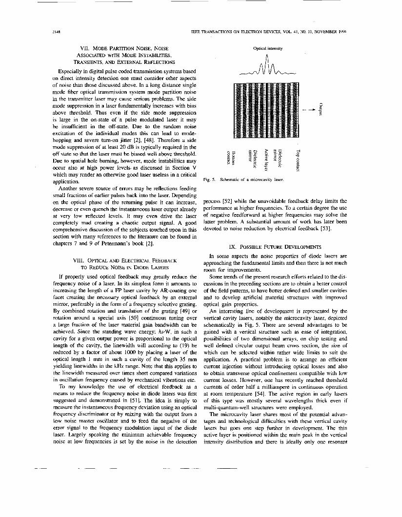
Optical intensity

Fig. 5. Schematic of a microcavity laser.

process [52] while the unavoidable feedback delay limits the performance at higher frequencies. To a certain degree the use of negative feedforward at higher frequencies may solve the latter problem. A substantial amount of work has later been devoted to noise reduction by electrical feedback [53].

IX. POSSIBLE FUTURE DEVELOPMENTS

In some aspects the noise properties of diode lasers are approaching the fundamental limits and then there is not much room for improvements.

Some trends of the present research efforts related to the discussions in the preceding sections are to obtain a better control of the field patterns, to have better defined and smaller cavities and to develop artificial material structures with improved optical gain properties.

An interesting line of development is represented by the vertical cavity lasers, notably the microcavity laser, depicted schematically in Fig. 5. There are several advantages to be gained with a vertical structure such as ease of integration, possibilities of two dimensional arrays, on chip testing and well defined circular output beam cross section, the size of which can be selected within rather wide limits to suit the application. A practical problem is to arrange an efficient current injection without introducing optical losses and also to obtain transverse optical confinement compatible with low current losses. However, one has recently reached threshold currents of order half a milliampere in continuous operation at room temperature [54]. The active region in early lasers of this type was mostly several wavelengths thick even if multi-quantum-well structures were employed.

The microcavity laser shares most of the potential advantages and technological difficulties with these vertical cavity lasers but goes one step further in development. The thin active layer is positioned within the main peak in the vertical intensity distribution and there is ideally only one resonant


mode of the optical cavity within the material gain bandwidth that couples effectively to the active layer. Since therefore a very large fraction of the spontaneous emission goes into the desired mode the threshold current becomes very low, ideally approaching zero [55]. Although the technological challenge to produce a practical device are formidable the underlying principles have already been verified experimentally and a substantial research effort with many leading laboratories involved is devoted to this development including studies of its fundamental noise properties [56].

Since all the presently used noise theories are based on the Langevin assumption that the individual processes of stimulated emission and absorption are uncorrelated one might speculate of how lasers will perform when this no longer holds, e.g., in the case of so short and intense optical pulses that Rabi oscillation phenomena become significant. Perhaps this will open up new fields of applied diode laser research involving highly nonlinear dynamic interaction between optical pulses.

Finally we will just mention a few words about the development of artificial material structures. These structures have geometrical dimensions of order electron wavelength which opens up the possibility to tailor electronic energy levels and the optical interaction characteristics to suite a given application. By using low dimensional structures called quantum wires and quantum dots one can thus, as mention in Section IV, reduce the coupling ( a ) between material gain and the real part of the refractive index so that these quantities may be controlled more independently which will greatly facilitate the realization of many laser optical functional devices.

X. FURTHER READING As a comprehensive introduction to the modulation and

noise properties of diode lasers Petermann’s book [2] is recommended. A good introduction to the quantum properties of electromagnetic fields is given in Marcuse’s book [33]. The most recent developments are usually reported in Electronic Letters, IEEE Photonic Technology Letters, Applied Physics Letters, Optic Letters, IEEE Journal of Quantum Electron- ics, IEEE Journal of Lightwave Technology, and Physical ReiYew A .

ACKNOWLEDGMENT

I would like to acknowledge valuable discussions with my coworkers at the Royal Institute of Technology, Stock- holm, Sweden: Eilert Berglind, Gunnar Bjork, Edgar Goobar, Anders Karlsson, and Richard Schatz. I also want to thank Bjame Tromborg at Telecommunications Research Laboratory, Horsholm, Denmark, for providing me with a collection of their recent papers and for interesting discussions.

REFERENCES

[ I ] H. Kogelnik and C. V. Schank, “Stimulated emission in a periodic structure,” Appl. Phys. Lett., vol. 18, pp. 152-154, 1971.

[2] K. Petermann, Laser Diode Modulation and Noise. Dordrecht, The Netherlands: Kluwer, 1991.

[3] Y. Yoshikuni, “Frequency tunability, frequency modulation and spectral linewidth of complicated structure lasers,” in Coherence, Amplification, and Quantum Effects in Semiconductor Lasers, Y. Yamamoto, Ed. New York: Wiley, 1991, chap. 4.

[4] H. Bissesur, “Effects of hole burning, carrier-induced losses and the camer-dependent differential gain on the static characteristics of DFB lasers,” J . Lightwave Technol., vol. IO, pp. 1617-1630, NOV. 1992.

[SI H. Haus, “Steady-state quantum analysis of linear systems,” Proc. IEEE, vol. 18. no. IO, pp. 1599-161 I , 1970.

[6] R. J . Glauber, “Coherent and incoherent states of the radiation field,” Phys. Rev., vol. 131, pp, 2766-2788, 1963.

[7] 0. Nilsson, A. Karlsson, and E. Berglind, “Modulation and noise spectra of complicated laser structures,” chap. 3 of 131.

[SI Haken, “Light,” vol. 2, Laser Light Dynamics. Amsterdam: Elsiever, 1985, chap. 7.

[9] K. Kurukawa, “Some basic characteristics of broadband negative resistance oscillator circuits,” Bell Syst. Tech. J . , vol. 48, pp. 1937-1953.

[lo] K. Uchida, “Phase noise in a laser with output coupling,” IEEE J . Quantum Electron., vol. QE-20, pp. 814-818, 1984.

[ I l l Y. Yamamoto and N. Imoto, “Internal and extemal field fluctuations of a laser oscillator: Part 1-uantum mechanical Langevin treatment”; 0. Nilsson, Y. Yamamoto and S. Machida, “Internal and external field fluctuations of a laser oscillator: Part 11-Electrical circuit theory,” IEEE J . Quantum Electron., vol. QE-22, pp. 2032-2052, 1986.

121 Y. Yamamoto, S. Machida, and 0. Nilsson, “Amplitude squeezing in a pump noise suppressed laser oscillator,” Phys. Rev. A, vol. 34, pp. 40254042, 1986.

131 W. H. Richardson, S. Machida, and Y. Yamamoto, “Squeezed photon number noise and sub-Poissonian electrical partition noise in a semiconductor laser,” Phys. Rev. Lerr., vol. 66, pp. 2867-2870, 1991.

141 J. Saltz, “Coherent lightwave communications,” AT&T Tech. J . , vol. 64, no. 10, p. 2164, 1985.

[IS] A. L. Schawlow and C. H. Townes, “Infrared and optical masers,” Phys. Rei,., vol. 112, pp. 1940-1949, 1958.

[I61 C. H. Henry, “Theory of the linewidth of semiconductor lasers,” IEEE J . Quantum Electron., vol. QE-18, pp. 259-264, 1982.

[ 171 M. Lax, “Classical noise V. Noise in self-sustained oscillators,” Phys. Rev., vol. 160, no. 2, pp. 29&307, 1967. Also H. Haug, H. Haken, Z. Physik, pp. 204 and 262, 1967.

[I81 M. Okai, M. Suzuki, and T. Taniwatari, “Strained multiquantum-well corrugation-pitch-modulated distributed feedback laser with ultranarrow (3.6 kHz) spectral linewidth,” Electronic Lett., vol. 29, no. 19, pp. 1696-1697, 1993.

[I91 K. Vahala and A. Yariv, “Detuned loading in coupled cavity semiconductor lasers-ffects on quantum noise and dynamics,” Appl. Phys. Left., vol. 45, no. 5 , pp. 501-503, 1984.

[20] C. H. Henry, “Theory of spontaneous emission noise in open resonators and its application to lasers and optical amplifiers,” J . Lighfwave Technol., vol. LT-4, no. 3, pp. 288-297, 1986.

[21] J. Arnaud, “Natural linewidth of anisotropic lasers,” Opt. and Quantum Electron., vol. 18, pp. 335-343, 1986.

[22] G. Bjork and 0. Nilsson, “A tool to calculate the linewidth of complicated laser structures,” IEEE J . Quantum Electron., vol. QE-23, pp. 1303-1312, 1987.

[23] J. Wang, N. Shunk and K. Petermann, “Linewidth enhancement for DFB lasers due to longitudinal field dependence in the laser cavity,” Electron. Lett., vol. 23, pp. 715-717, 1987.

[24] B. Tromborg, H. Olesen, X. Pan, and S. Saito, “Transmission line description of optical feedback and injection locking for Fabry-Perot and DFB lasers,” IEEE J . Quantum Elecftvn., vol. QE-23, pp. 1875-1889, 1987.

[25] H. Haus, “On the excess spontaneous emission factor,” in gain-guided laser amplifiers, IEEE J . Quantum Electron., vol. QE-21, pp. 63-69, 1985.

[26] A. E. Siegman, “Excess spontaneous emission in non-Hermitian optical systems,” Phys. Rev. A, vol. 39, pp. 1253-1268, 1989.

[27] K. Petermann, “Calculated spontaneous emission factor for double- heterostructure injection lasers with gain-induced waveguiding,” IEEE J . Quantum Electron., vol. QE-IS, pp. 566-570, 1979.

[28] M. C. Amman, “Linewidth enhancement in distributed feedback semiconductor lasers,” Electron. Lett., vol. 26, pp. 569-571, 1990.

[29] T. L. Koch and U. Koren, “Semiconductor lasers for coherent optical fiber communications,” J . Lightwalv Technol., vol. LT-8, pp. 274-293, Mar. 1990.

[30] A. J. Lowery, “New dynamic model for multimode chirp in DFB semiconductor lasers,” IEE Proc. J . , vol. 137, no. 5 , pp. 293-230, 1990.

[31] B. Tromborg, H. E. Lassen, and H. Olesen, ‘‘Traveling wave analysis of semiconductor lasers: Modulation responses, mode stability and quantum mechanical treatment of noise spectra,” IEEE J . Quantum E/ec.rron., vol. 30, Apr. 1994.

[32] A. Imamoglu and Y. Yamamoto, “Noise suppression in semiconductor p - n junctions: Transition from macroscopic squeezing to mesoscopic

IEEE TRANSACTIONS ON ELECTRON DEVICES, VOL. 41, NO. 11, NOVEMBER 1994

coulomb blockade of electron emission processes,” Phys. Rev. Lett., vol. 70, no. 21, pp. 3327-3331, 1993. D. Marcuse, Principles of Quantum Electronics. New York Academic, 1980. A. Karlsson and G. Bjork, “Use of quantum noise correlation for noise reduction in semiconductor lasers,” Phys. Rev. A, vol. 44, no. 11, pp. 7669-7683, 1991. M. C. Teich and B. Saleh, “Squeezed states of light,” Quantum Optics,

A. Karlsson, R. Schatz, and 0. Nilsson, “Modulation and noise properties of multi-element semiconductor lasers,” in A. Karlsson; “Quantum noise in semiconductor lasers and amplifiers,” ISRN KTHIMVTlFR-91I2- SE, Royal Institute of Technol., Stockholm, 1991. S. Machida, Y. Yamamoto, and Y. Itaya, “Observation of amplitude squeezing in a constantcurrent-driven semiconductor laser,” P hys. Rev. Lett., vol. 58, pp. 1000-1003, 1987. E. Goobar, “A Michelson interferometer with balanced detection for the characterisation of modulation and noise properties of semiconductor lasers,” IEEE J. Quantum Electron., vol. 29, pp. 11 16-1 130, 1993. T. Okoshi, K. Kikuchi, and A. Nakagama, “Novel method for high resolution measurement of laser out put spectrum,” Electron. Lett., vol. 16, pp. 630-631, 1980. H. A. Haus and J. A. Mullen, “Quantum noise in linear amplifiers,” Phys. Rev., vol. 128, pp. 2407-2413, 1962. C. M. Caves, “Quantum limits on noise in linear amplifiers,” Phys. Rev.

vol. 1, pp. 153-191, 1989.

D, vol. 26, pp. 1817-1839, 1982. 1 N. A. Olsson, “Lightwave systems with optical amplifiers,”J. Lightwave

Technol., vol. 7, pp. 1071-1082, July 1989. E. Berglind and L. Gillner, “Optical quantum noise treated with classical electrical network theory,” IEEE J. Quantum Electron., vol. 30, pp. 846853, 1994.

1 T. Li and M. C. Teich, “Photon point process for traveling-wave laser amplifiers,” IEEE J. Quantum Electron., vol. 29, pp. 2568-2578, 1993.

1 P. J. Edwards, “Low-noise optoelectronic amplifier using sub-shot noise light,” Electron. Lett., vol. 29, pp. 299-301, 1993.

[46] E. Goobar, A. Karlsson, and G. Bjork, “Experimental realisation of a semiconductor photo number amplifier and a quantum optical tap,” and J.-F. Roch, J.-Ph. Poizat, and P. Grangier, “Sub-shot-noise manipulation of light using semiconductor emitters and receivers,” Phys. Rev. Lett., vol. 71, no. 13, pp. 2002-2009, 1993.

[47] 0. Nilsson, A. Karlsson, E. Goobar, and G. Bjork, “Photon number amplification in a multijunction single mode laser cavity,” in Proc. CLEO IQEC ’94, paper QWF4, Anaheim, CA, May 1994.

[48] P. 0. Andersson and K. &ermark, “Generation of BER floors from laser diode chirp noise,” Electron. Lett., vol. 28, pp. 472-473, 1992.

I491 F. Favre, D. le Guen, J. C. Simon, and B. Landouises, “External cavity

laser with 15 nm continuous tuning range,” Electron. Lett., vol. 22, pp.

[50] 0. Nilsson, E. Goobar, and K. Vilhelmson, “Continuously tuneable external-cavity laser,” P roc. 16th Europe. Con$ on Optical Commun., Amsterdam, 1990, pp. 373-376.

[51] S. Saito, 0. Nilsson, and Y. Yamamoto, “Frequency modulation noise and linewidth reduction by means of a negative frequency feedback technique,” Appl. Phys. Lett., vol. 46, pp. 3-5, 1985.

[52] Y. Yamamoto, 0. Nilsson, and S. Saito, “Theory of a negative frequency feedback semiconductor laser,” IEEE J . Quantum Electron., vol. QE-21,

[53] M. Ohtsu and K. Nakagawa, “Spectroscopy by semiconductor lasers,” chap. 5 of [3].

[54] R. S. Geels and L. A. Coldren, “Submilliamp threshold vertical-cavity laser diodes,” Appl. Phys. Lett., vol. 57, no. 16, pp. 1605-1608, 1990.

[55] F. De Martini and G. R. Jacobovitz, “Anomalous spontaneous stimulated decay. Phase transition and zero-threshold laser action in a microscopic cavity,” Phys. Rev. Letr., vol. 60, no. 17, pp. 1711-1714, 1988.

[56] Y. Yamamoto, S. Machida, and G. Bjork, “Microcavity semiconductor laser with enhanced spontaneous emission,” Phys. Rev. A, vol. 44, no. 1, pp. 657-668, 1991.

1795-1796, 1986.

pp. 1919-1928, 1985.

B. Olle Nilsson was born in Goteborg, Sweden, on October 25, 1934. He received the Civ. Ing. degree and the Tekn. Dr. degree in electrical engineering from Chalmers University of Technology, Goteborg, in 1959 and 1968, respectively.

From 1968 to 1984 he was with Chalmers Univer- sity of Technology, where he worked in microwave engineering as well as laser optics and thermionic energy conversion. From 1984 to 1991 he was Chairman and Professor in the Microwave Engi- neering and Fiber Optics Department at the Royal

Institute of Technology, Stockholm, Sweden, where his research focused on high-speed fiber optical telecommunication. During 1987-1988 he was a Vis- iting Researcher at the NTT Basic Research Laboratories, Musashino, Japan, working with diode lasers and fundamental quantum mechanical aspects of laser noise. Since 1991 he has been with Ellemtel Telecommunication Systems Laboratories as a Scientific Adviser studying physical pnnciples for future broadband telecommunication. In 1991 he also became Adjunct Professor in Photonics ana Microwave Engineenng at Chalmers University of Technology and at the Royal Institute of Technology.

Date post:	21-Sep-2016
Category:	Documents
Upload:	bo
View:	214 times
Download:	0 times

Noise mechanisms in laser diodes

Documents